| Issue |
A&A
Volume 697, May 2025
|
|
|---|---|---|
| Article Number | A86 | |
| Number of page(s) | 25 | |
| Section | Extragalactic astronomy | |
| DOI | https://doi.org/10.1051/0004-6361/202453172 | |
| Published online | 12 May 2025 | |
HI within and around observed and simulated galaxy discs
Comparing MeerKAT observations with mock data from TNG50 and FIRE-2
1
INAF – Padova Astronomical Observatory, Vicolo dell’Osservatorio 5, I-35122 Padova, Italy
2
The Netherlands Institute for Radio Astronomy (ASTRON), Oude Hoogeveensedijk 4, 7991 PD Dwingeloo, The Netherlands
3
Dept. of Astronomy, Univ. of Cape Town, Private Bag X3, Rondebosch 7701, South Africa
4
Kapteyn Astronomical Institute, University of Groningen, PO Box 800, 9700 AV Groningen, The Netherlands
5
INAF – Osservatorio Astronomico di Cagliari, Via della Scienza 5, 09047 Selargius, (CA), Italy
6
Institute for Computational Cosmology, Durham University, South Road, Durham DH1 3LE, UK
7
Centre for Extragalactic Astronomy, Durham University, South Road, Durham DH1 3LE, UK
8
Department of Physics, Durham University, South Road, Durham DH1 3LE, UK
9
Observatoire de Paris, LERMA, Collège de France, CNRS, PSL University, Sorbonne University, 75014 Paris, France
10
Department of Astronomy, Case Western Reserve University, 10900 Euclid Avenue, Cleveland, OH 44106, USA
11
Ruhr University Bochum, Faculty of Physics and Astronomy, Astronomical Institute (AIRUB), 44780 Bochum, Germany
12
Department of Physics, Engineering Physics and Astronomy, Queen’s University, Kingston, ON K7L 3N6, Canada
13
Aix Marseille Univ, CNRS, CNES, LAM, Marseille, France
14
Universidad Andrés Bello, Facultad de Ciencias Exactas, Departamento de Ciencias Físicas – Instituto de Astrofísica, Fernandez Concha 700, Las Condes, Santiago, Chile
15
Centre for Astrophysics Research, University of Hertfordshire, College Lane, Hatfield AL10 9AB, UK
⋆ Corresponding author: This email address is being protected from spambots. You need JavaScript enabled to view it.
Received:
26
November
2024
Accepted:
3
March
2025
Abstract
Extragalactic gas accretion and outflows driven by stellar and active galactic nucleus (AGN) feedback are expected to influence the distribution and kinematics of gas in and around galaxies. Atomic hydrogen (H I) is an ideal tracer of these processes, and it is uniquely observable in nearby galaxies. Here we made use of wide-field (1° ×1°), spatially resolved (down to 22″), high-sensitivity (∼1018 cm−2) H I observations of five nearby spiral galaxies with stellar mass of ∼5 × 10¹⁰ M⊙, taken with the MeerKAT radio telescope. Four of these were observed as part of the MHONGOOSE survey. We characterise the main H I properties in regions of a few hundred kiloparsecs around the discs of these galaxies, and compare them with synthetic H I data from a sample of 25 similarly massive star-forming galaxies from the TNG50 (20) and FIRE-2 (5) suites of cosmological hydrodynamical simulations. Overall, the simulated systems have H I and molecular hydrogen (H2) masses in good agreement with the observations, but only when a pressure-based H2 recipe is employed. The other recipes that we tested overestimate the H2-to-H I mass fraction by up to an order of magnitude. On a local scale, we find two main discrepancies between the observed and simulated data. First, the simulated galaxies show a more irregular H I morphology than the observed galaxies, due to the presence of H I with column density < 1020 cm−2 up to ∼100 kpc from the galaxy centre, even though they inhabit more isolated environments than the observed targets. Second, the simulated galaxies and in particular those from the FIRE-2 suite, feature more complex and overall broader H I line profiles than the observed galaxies. We interpret this as being due to the combined effect of stellar feedback and gas accretion, which lead to a large-scale gas circulation that is more vigorous than in the observed galaxies. Our results indicate that, with respect to the simulations, gentler processes of gas inflows and outflows are at work in the nearby Universe, leading to more regular and less turbulent H I discs.
Key words: accretion / accretion disks / methods: numerical / galaxies: halos / galaxies: kinematics and dynamics / galaxies: spiral
© The Authors 2025
 Open Access article, published by EDP Sciences, under the terms of the Creative Commons Attribution License (https://creativecommons.org/licenses/by/4.0), which permits unrestricted use, distribution, and reproduction in any medium, provided the original work is properly cited.
This article is published in open access under the Subscribe to Open model. This email address is being protected from spambots. You need JavaScript enabled to view it. to support open access publication.
1. Introduction
The build-up of galaxies in the field environment can be thought of as the competition between the ‘positive’ process of cooling and gravitational collapse of gas within the potential wells provided by dark matter (DM) halos (White & Rees 1978), and a series of ‘negative’ mechanisms such as gas heating and subsequent expulsions caused by feedback from star formation (Larson 1974; Dekel & Silk 1986) and active galactic nuclei (AGN; Silk & Rees 1998; Harrison 2017). This competition produces a continuous exchange of gas between the galaxy and its host halo, ultimately regulating the main properties (mass, angular momentum, chemical composition) of the interstellar medium (ISM), the material from which stars form and supermassive black holes grow.
The study of this galaxy-halo interplay is pivotal in order to shed light on a number of open issues in galaxy evolution theory. Total gas consumption timescales in present-day galaxies are of the order of a few gigayears (Kennicutt 1998; Leroy et al. 2013) and become even shorter at higher redshift (Saintonge et al. 2013), providing indirect but compelling evidence for the existence of a continuous gas supply that replaces the material used for star formation processes (Fraternali & Tomassetti 2012). Cosmological simulations in a Lambda-cold dark matter (ΛCDM) framework identify such a supply in the form of cold (105 K) gas filaments either inflowing directly onto galaxies from the cosmic web (cold-mode accretion) or shock-heated to the halo virial temperature into a diffuse, extended gas reservoir, sometimes called the corona (hot-mode accretion,e.g., Kereš et al. 2005; Nelson et al. 2013; Ramesh et al. 2023).
However, direct evidence of gas accretion onto galaxies, at least in the local Universe where the most sensitive data are available, is scarce. Wet mergers can only provide a small fraction of the accretion rate required to balance the galaxy star formation rate (Sancisi et al. 2008; Di Teodoro & Fraternali 2014). The same applies for the supply provided by the direct infall of isolated optically dark H I clouds detected in the halos of galaxy discs (Kamphuis et al. 2022). Cosmological cold accretion is expected to produce relatively strong inward radial motions at the periphery of discs (e.g. Trapp et al. 2022), which seem to be elusive in observations (Di Teodoro & Peek 2021). While the expected radiative cooling rate of the hot corona is largely insufficient to match the star formation rate in galaxies like the Milky Way (e.g. Miller & Bregman 2015), whether or not cold gas clouds can spontaneously form within the corona and precipitate onto the disc is a highly debated topic (Binney et al. 2009; Nipoti 2010; Voit et al. 2017; Sobacchi & Sormani 2019; Afruni et al. 2023). Hence, an important point to address is how and where gas accretion onto galaxies takes place. A possibility could be that the cooling of the coronal gas is limited to a region that is a few kiloparsec thick surrounding the star formation disc (e.g. Stern et al. 2024). The cooling of the coronal gas can be favoured by the interaction with material ejected from the galaxy by supernova feedback (a galactic fountain), which produces a gas mixture with temperature, density, and metallicity intermediate between those of the corona and of the ISM, and thus with a short cooling time (< 100 Myr) (Marinacci et al. 2010; Fraternali 2017). This process is expected to leave a subtle, but detectable, imprint on the kinematics of the H I at the disc–corona interface, characterised by a lagging rotation and an overall inflow motion in the vertical and radial directions. This can be exploited to infer the condensation rate of the coronal gas via the modelling of highly sensitive spatially resolved H I observations (Fraternali & Binney 2008; Marasco et al. 2012; Li et al. 2023).
Galactic winds triggered by star formation or AGN feedback are thought to play a key role in setting two important properties of the observed galaxy population. One is the low overall star formation efficiency: galaxies are unable to convert the majority of baryons associated with their DM halos into stars, with an efficiency that peaks in local L⋆ galaxies and rapidly declines for lower and higher luminosities (e.g. Moster et al. 2013; Behroozi et al. 2013). Thus, most baryons in dark matter halos are not in the form of stars and the ISM, but in a more diffuse circumgalactic medium (CGM). The other property is the specific angular momentum (j) distribution (AMD) of stars and gas within galaxies. Most star-forming galaxies across all redshifts appear as disc-like, rotationally supported structures, and therefore are characterised by an AMD that lacks very low-j material. Instead, typical dark matter halos in ΛCDM cosmological simulations have an excess of low angular momentum material compared to galaxy discs (e.g. Bullock et al. 2001). If dark matter and baryons in halos follow the same AMD (Sharma & Steinmetz 2005), this mismatch implies a biased assembly, where galaxies have been forming their stars preferentially using the high-j reservoir available in their halo. These two properties can be explained by powerful galactic winds that preferentially remove the low-j star-forming material from the galaxy, thus lowering the star formation efficiency, while promoting the build-up of galaxy discs.
Galaxy-scale outflows are routinely observed at all redshifts using a variety of different tracers (e.g. Veilleux et al. 2005; Rubin et al. 2014; Woo et al. 2016; Cicone et al. 2018). However, robust measurements of the properties of the galactic wind, such as speed and mass outflow rate, have proved to be challenging due to the complex geometry and multi-phase nature of the phenomenon, often leading to different estimates depending on the method adopted (e.g. Chisholm et al. 2017; McQuinn et al. 2019; Concas et al. 2022; Marasco et al. 2023). On the other hand, theoretical predictions for the wind properties vary depending on the model considered, with large-scale cosmological simulations in the ΛCDM framework typically predicting more extreme winds (e.g. Nelson et al. 2019a; Mitchell et al. 2020) compared to small-scale simulations of the ISM (e.g. Kim & Ostriker 2018) or to chemical evolutionary models (e.g. Camps-Fariña et al. 2023; Kado-Fong et al. 2024).
We can summarise the scenario described above as follows: first, there are strong theoretical arguments and compelling indirect evidence, but very little observational support, for the need for gas accretion onto galaxies; second, the feedback efficiency required by cosmological simulations is in tension with several observational constraints and small-scale simulations. These tensions are caused, at least in part, by two limitations. First, there exists a gap between hydrodynamical models of galaxy evolution and observations in terms of comparison strategy, as models were often used to derive physical quantities that could not readily be measured observationally. The situation has drastically improved in the last few years (e.g. Marasco et al. 2018; Oman et al. 2019; Faucher et al. 2023; Gebek et al. 2023; Baes et al. 2024) thanks to the level of sophistication reached by present-day models, which permit the production of synthetic (broad-band or emission-line) observations, incorporating all of the limitations of the desired facilities such as sensitivity, resolution and field of view, providing a more direct and straightforward comparison with the data. Second, there exists an observational limitation due to the intrinsically low-density nature of the material involved in the gas circulation processes, which demands very deep observations to make its analysis possible (e.g. Popping et al. 2009). If we limit the discussion to the atomic hydrogen (H I) phase, which is the subject of our study, there is general agreement between different simulation suites that the large-scale filamentary structure of the gas accreting from the cosmic web can be revealed only by pushing the H I column density (NHI) sensitivity below values of ≃1019 cm−2 (van de Voort et al. 2019; Ramesh et al. 2023). Single-dish radio observations can easily reach such sensitivities and have shown that H I with NHI < 1019 cm−2 makes up to ∼2% of the total H I mass budget in and around nearby star-forming galaxies (e.g. Pingel et al. 2018). Clearly, radio-interferometric observations are crucial in order to infer the spatial distribution and kinematics of the low column density H I, but the sensitivity required was hardly achievable until today.
This study is an attempt to overcome both of these limitations by combining ultra-deep spatially resolved H I observations of five nearby galaxies, similar to the Milky Way (MW) in terms of baryonic mass and SFR, taken with the MeerKAT radio telescope, with synthetic H I data of similarly massive spirals extracted from two widely studied suites of hydrodynamical simulations in the ΛCDM framework, Illustris TNG50 (Pillepich et al. 2019; Nelson et al. 2019b) and FIRE-2 (Hopkins et al. 2018a). We focus on MW-like objects alone, as we expect them to feature substantial ongoing gas inflows and outflows due to their relatively short gas consumption timescales (in contrast with lower mass galaxies, e.g. McGaugh et al. 2017), an argument which is strongly supported by different hydrodynamical simulations of galaxy evolution in the MW-like mass regime (e.g. Fernández et al. 2012; van de Voort et al. 2019; Trapp et al. 2022). The use of two different simulation prevents us from being biased towards a particular model. The focus on the H I emission line is justified by the fact that, even though this phase is not expected to dominate the mass budget of the CGM (unless we limit our study to a region of a few kpc around the disc, see Marasco et al. 2019), H I observations with MeerKAT combine depth, resolution, and field of view to provide a unique, broad picture of the disc-halo interplay. Our goal is twofold. On the one hand the comparison will furnish insights into the physical interpretation of specific features detected in the data. On the other hand it will capture the main differences between the models and the data, which gives us clues to how the former can be refined.
This paper is structured as follows. In Section 2 we provide a description of the observed and simulated galaxy samples used, and of the approach adopted to build synthetic H I datacubes (‘mocks’) from the models. In Section 3 we show our main results, highlighting the main differences between the data and the mocks in terms of column density and velocity dispersion distributions. Section 4 focuses on our understanding of the origins of the difference found in terms of environment, stellar feedback, and gas accretion rates. We summarise our results and present our conclusions in Section 5.
2. Galaxy samples
Our strategy is to focus on regular star-forming galaxies with stellar masses comparable to those of the Milky Way, as for these systems we expect a more active disc-halo gas circulation due to their relatively low gas consumption timescales. Our selection criteria for the simulated galaxy samples are based on this strategy. On the observational side, our analysis is limited by the paucity of ultra-deep, spatially resolved HI observations for galaxies with the required properties. To our knowledge, the observed subsample used for our study is the best compromise that we can currently achieve in terms of HI data quality and required galaxy properties.
2.1. The observed sample
Our observed galaxy sample is formed by five objects whose main properties are listed in Table 1. With the exception of J0342-47, all galaxies were observed as a part of the MeerKAT H I Observations of Nearby Galactic Objects – Observing Southern Emitters (MHONGOOSE) survey (de Blok et al. 2024, hereafter dB24).
Main properties of the five galaxies observed with MeerKAT and analysed in this study.
MHONGOOSE is a MeerKAT Large Survey Project aimed at providing ultra-deep, spatially resolved H I observations of 30 nearby (D ≲ 20 Mpc), galaxies outside clusters and major groups in the Southern hemisphere, covering a wide range of stellar and H I masses (6.0 < log10(M⋆/ M⊙) < 10.7, 7.0 < log10(MHI/ M⊙) < 10.3). The goal of MHONGOOSE is to probe the H I cycle between galaxy discs and their circumgalactic media and study its connection to star formation feeding and feedback processes. To achieve this, MHONGOOSE exploits both the large FoV of MeerKAT, with a primary beam FWHM at 1.4 GHz of ∼1° (corresponding to 350 kpc at a distance D = 20 Mpc), and its outstanding multi-resolution performance, reaching a minimum H I column density sensitivity (3σ integrated over a velocity width of 16 km s−1) of 6 × 1017 cm−2 for a beam FWHM of 90″ (8.6 kpc at D = 20 Mpc) for emission that is more extended than this resolution. The sensitivity is better than 1020 cm−2 up to the highest resolution achievable, 7.6″ (0.74 kpc at D = 20 Mpc). The unique combination of area, sensitivity and resolution makes MHONGOOSE the optimal survey to study faint H I features in and around galaxy discs.
As in this study we focussed on galaxies with M⋆ similar to that of the MW, we were limited to the four most massive galaxies available in MHONGOOSE: J0335-24, J0052-31, J0419-54 and J0445-59 (see Table 1 for the NGC identifications). These are the only MHONGOOSE galaxies with M⋆ > 1010 M⊙ and have distances of ∼20 Mpc, which implies that the MeerKAT FoV covers approximately the virial region, assuming typical dark matter halos analogous to that of the MW (e.g. Posti & Helmi 2019). Also, we limited our analysis to two of the six standard resolutions available in the survey, a high-resolution (HR) case, with beam FWHM of ∼22″ (∼2 kpc) and nominal column density sensitivity (3σ over 16 km s−1) of 5 × 1018 cm−2, and a low-resolution (LR) case with beam FWHM of ∼65″ (6.3 kpc) and sensitivity of ∼1018 cm−2. These two resolutions correspond, respectively, to the r10_t00 and r05_t60 configurations presented in dB24. Table 2 lists the main datacube parameters associated with these two resolution cases, which will be adopted also for the realisation of synthetic H I data for the simulated galaxy samples (see Section 2.3).
Characteristic parameters for the H I datacubes of the observed and simulated galaxy samples.
In addition to these four MHONGOOSE systems, we added a fifth MW-like galaxy, J0342-47 (or NGC 1433). This is a Seyfert galaxy that has stellar mass and distance compatible with the other galaxies in our sample (see Table 1), and is characterised by a central outflow visible in both the molecular (Combes et al. 2013) and the ionised (Arribas et al. 2014) phase driven by its AGN. J0342-47 was observed for ten hours with MeerKAT as a part of the MKT-20202 project (PI: F. Maccagni). A channel width of 5.51 km s−1 was used for the data reduction, providing a column density limit about 18 per cent higher than those reported in our Table 2 for the same resolution cases.
Fig. 1 shows the primary-beam corrected moment-0 (column density, NHI) and moment-2 (velocity dispersion, σ)1 H I maps for the five MeerKAT galaxies and for both the resolution cases studied, together with gri colour-composite images from the data release 10 of the DESI Legacy Imaging Surveys (Dey et al. 2019). The H I maps were derived using the SoFia-2 software package (Westmeier et al. 2021) as discussed in dB24. We refer to that paper for more details; here we describe the basic procedure. The SoFiA-2 smooth and clip (S+C) method was used to find significant voxels in the cubes using spatial kernels of zero and four pixels and velocity kernels of zero, nine and 25 channels using a threshold of 4σrms. Detected voxel regions were then linked over a maximum of five pixels spatially and eight channels spectrally (two channels in J0342-47). A minimum size of four spatial pixels and 15 channels was then imposed on these linked regions. The SoFiA reliability parameter was used to further identify significant sources in the cube. However, as mentioned in dB24, the value adopted for this parameter was not crucial as almost all sources were well separated from the noise, thanks to the high S/N of the MHONGOOSE data. The significant sources were extracted using a reliability value of 0.8 and requiring an integrated S/N value of five.
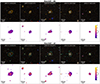 |
Fig. 1. MeerKAT galaxy sample studied in this work. The high-resolution (∼22″) and low-resolution (∼65″) cases (HR and LR) are shown separately in the top and bottom parts of the figure. Top panels: H I column density iso-contours overlaid on top of grz colour-composite images from the DESI Legacy Imaging Surveys (Dey et al. 2019). Contours are drawn from primary-beam corrected moment-0 maps at NHI levels of 1019, 1020 (thicker line), 1020.5, and 1021 cm−2. The LR panels show an additional contour at the level of 1018 cm−2, in cyan. Bottom panels: Moment-2 maps. The velocity colour scheme is shown in the rightmost panels. |
The detailed H I morphology and kinematics of these five galaxies will be investigated elsewhere. Here, we remark on a striking feature of these observations, which is the lack of diffuse H I emission around the galaxies. Virtually all of the H I visible around the main targets is in the form of H I-bearing satellites. In addition, all galaxies feature relatively low σ values ranging from 8 to 30 km s−1, with the exception of their central region, where σ increases due to beam-smearing effects and to the probable presence of outflows driven by feedback from an Active Galactic Nucleus (AGN), as the majority of the systems in the observed sample are known Seyfert galaxies. The amount of H I in the CGM and the H I velocity dispersion are the two main features that will be contrasted with predictions from the simulations in this study.
2.2. The simulated sample
We focused on two different state-of-the-art simulation suites: Illustris TNG50 (Pillepich et al. 2019; Nelson et al. 2019a) and FIRE-2 (Hopkins et al. 2018b). TNG50 is a cosmological, magneto-hydrodynamical simulation of galaxy formation and evolution in a ΛCDM universe (Planck Collaboration XIII 2016), made using the moving-mesh code AREPO (Springel 2010; Weinberger et al. 2020) and adopting the fiducial Illustris TNG galaxy formation model (Weinberger et al. 2017; Pillepich et al. 2018). It follows the evolution of dark matter, gas, stars, supermassive black holes (SMBHs) and magnetic fields in a ∼(50 Mpc)3 cubic (co-moving) volume down to z = 0, with a maximum resolution2 of ∼70 pc and gas particle mass of 8.5 × 10⁴ M⊙. Amongst the different astrophysical processes modelled, TNG50 includes primordial and metal-line cooling down to 104 K, heating from a spatially homogeneous UV/X-ray background, galactic-scale stellar-driven outflows, and the seeding, growth and feedback of SMBHs. The cold and dense phase of the ISM is not directly resolved in TNG50, and star-forming gas is treated following the prescriptions of Springel & Hernquist (2003) which employ a two-phase, effective equation-of-state model.
In this study, we considered galaxies from the MW- and Andromeda-like (MW/M31-like) TNG50 sample recently presented by Pillepich et al. (2024, see also Ramesh et al. 2023). This sample is made of 198 grand design spiral galaxies, with M⋆ in the range 1010.5 − 11.2 M⊙, and within a MW-like large-scale environment at z = 0. The latter condition ensures the absence of massive (M⋆ > 1010.5) companions within 500 kpc from the main galaxy, and having host halo masses below those of typical galaxy groups (M200 < 1013 M⊙), which qualitatively matches the environment of galaxies in MHONGOOSE. From this sample we randomly extracted 20 systems with a SFR that falls within ±0.5 dex of the SFR-M⋆ relation of Chang et al. (2015), to ensure star formation properties similar to those of similarly massive galaxies in the local Universe. Additionally, we applied a further cut to ensure a minimum H I mass of 109.5 M⊙, similar to that of J0342-47, the most H I-poor galaxy of our observed sample (log10(MHI/ M⊙) = 9.43 ± 0.08 assuming a distance of 18.63 ± 1.86 Mpc, from Anand et al. 2021). Details on the computation of H I masses for the simulated galaxies are provided below. The main properties of these 20 objects are listed in Table 3.
Main properties of the simulated systems studied in this work.
The FIRE-2 suite is a collection of zoom-in hydrodynamical simulations performed with the mesh-less finite-mass (MFM) method implemented in the GIZMO (Hopkins 2015) code. FIRE-2 simulations reach parsec-scale resolution to explicitly model the multiphase interstellar medium while implementing direct models for stellar evolution and feedback mechanisms. These include energy and momentum injection from stellar winds, core-collapse and Type Ia supernovae, momentum flux from radiation pressure, photoionization and photoelectric heating. The so-called core FIRE-2 suite (Wetzel et al. 2023) follows the evolution of 23 galaxies with stellar mass M⋆ between 104 and 1011 M⊙ down to z = 0, with a particular focus on MW-like systems, which form most (14/23) of the sample. In contrast with TNG50, none of the FIRE-2 simulations model feedback from AGN, which may cause MW-like galaxies to form overly massive bulges and play a role in their elevated star formation rates at low z, as we discuss below. Given their higher resolution and lack of pre-computed H I fractions (see Section 2.3), FIRE-2 snapshots are much more computationally demanding to process with our routines than TNG50 ones. For this reason, we limited our analysis to five MW-like systems from the core suite, randomly selected among those with the poorest resolution (gas particle mass of 7100 M⊙), which is still more than a factor of ten better than TNG50. The main properties of these systems are listed in Table 3.
In both TNG50 and FIRE-2, the fraction of neutral3 hydrogen associated with each gas particle (fn) is regulated by photoionization and heating from a redshift-dependent, spatially uniform ultraviolet (UV) background (from Faucher-Giguère et al. 2009). Self-shielding for high-density gas follows the prescription of Rahmati et al. (2013a) in TNG50, or is directly computed using the local (averaged over the Jeans length) gas column density and opacity in FIRE-2 (Faucher-Giguère et al. 2015). Although these calculations do not account for local stellar radiation leaking from star-forming regions in the host disc, we expect this to affect H I fraction estimates only for column densities NHI ≥ 1021 cm−2 (Rahmati et al. 2013b; Gebek et al. 2023).
Finally, neutral hydrogen masses must be partitioned into atomic (H I) and molecular (H2) components. TNG50 snapshots from the MW/M31 sample have pre-computed H2 fractions from three different recipes: Blitz & Rosolowsky (2006, hereafter BR06), Gnedin & Kravtsov (2011, GK11) or Krumholz (2013, K13). These recipes provide different approaches to the modelling of the atomic-to-molecular transition in hydrodynamical simulations. The BR06 recipe is based on the observed correlation between the H2 fraction and the midplane pressure, whereas the other two are based on different observables, such as the gas surface density and metallicity, and are either fully analytical (K13) or calibrated on high-resolution simulations of isolated disc galaxies (GK11). Diemer et al. (2018) provide further details on the modelling of the H I-to-H2 transition in hydrodynamical simulations.
We applied these prescriptions also to FIRE-2 snapshots. For the GK11 and K13 recipes, we used the PYTHON implementation provided by Adam R. H. Stevens4, which are detailed in Stevens et al. (2019). Similarly to Marinacci et al. (2017), we implemented the BR06 scheme by computing Rmol, the ratio of the H2 mass to the H I mass of each gas particle or cell, as
 (1)
(1)
where fn is the neutral gas fraction, P is the pressure associated with the gas particle or cell, P0 = 1.7 × 10⁴ K cm−3, and α = 0.8 as found by Leroy et al. (2008). Although the details of the implementation of the BR06 scheme vary from one study to another (e.g. Bahé et al. 2016; Diemer et al. 2018), they have a very small impact on the distribution and kinematics of the low-NHI gas that resides at the periphery of galaxy discs, where the H2 fraction is typically negligible.
Fig. 2 shows the ratio between H2 and H I total masses computed in a sphere with 100 kpc of radius from the centre of all simulated galaxies, and compares it with measurements from the GALEX Arecibo SDSS Survey (xGASS, Catinella et al. 2018). The prescription of BR06 is the one that better reproduces the observed molecular-to-atomic hydrogen mass ratio, and it will be the fiducial prescription adopted for the rest of this work. A similar conclusion was already reached by Bahé et al. (2016) studying H I discs in the EAGLE simulations (Schaye et al. 2015). Although more recent works have preferred to use the other prescriptions (e.g. Ramesh et al. 2023; Arabsalmani et al. 2023), Fig. 2 shows that these overestimate the H2-to-H I mass fractions by about an order of magnitude, thus we advise against their use to infer the atomic and molecular gas budget in simulated galaxies from the TNG50 and FIRE-2 suites, at least in the mass range explored here. A 100 kpc aperture is adequate to encompass the very extended H I disc of some of the TNG50 galaxies (e.g. 520885), but using a smaller aperture radius of 50 or 25 kpc would only strengthen our results, given that the H2 is more centrally concentrated than the H I, causing MH2/MHI to increase for decreasing aperture radii. We stress that, as expected, the various recipes affect the H I fractions at NHI > 1020 cm−2 but have no impact on the low-density CGM gas, where all neutral hydrogen is in the atomic phase (Figure A.3). In addition, we verified the validity of a simpler partition scheme for FIRE-2 systems based on straight temperature and density cuts (fH2 = 1 for gas with T < 30 K and nH > 10 cm−3, fH2 = 0 otherwise). This scheme has been adopted in previous studies of FIRE-2 galaxies (Orr et al. 2018; Sands et al. 2024) and leads to H I masses that are larger than those determined using the Blitz & Rosolowsky (2006) recipe by 0.16 dex.
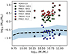 |
Fig. 2. Molecular-to-atomic hydrogen mass ratio as a function of galaxy stellar mass for the TNG50 (circles) and FIRE-2 (stars) systems studied in this work. All masses are computed within 100 kpc from the galaxy centre. Different H2/H I partition recipes are shown with different colours: green for Gnedin & Kravtsov (2011, GK11), red for Krumholz (2013, K13), and blue for Blitz & Rosolowsky (2006, BR06). The recipe of BR06 is the one that best reproduces the observational values from the xGASS Survey (Catinella et al. 2018), which are represented here by the shaded region. |
The main properties of the simulated galaxies from Table 3 are compared with those of various observational datasets in Fig. 3. We caution that the observational measurements in Fig. 3 are taken from the literature and make use of a variety of methods applied to different datasets. Masses and SFRs of simulated galaxies were derived within 100 kpc from their centre, using the properties of the stellar particles in the snapshots. In particular, SFRs were determined from the total birth mass of the stars younger than 100 Myr, to match the typical timescales of the SFR tracers (UV and mid-IR) used for the MHONGOOSE galaxies (see dB24). All FIRE-2 galaxies are located above the main sequence of star formation, as derived by Chang et al. (2015) from Sloan Digital Sky Survey (SDSS York et al. 2000) data, which is likely a consequence of the lack of AGN feedback in the FIRE-2 models. TNG50 galaxies, instead, are more compatible with the SDSS, the MHONGOOSE and HALOGAS samples. The right panel of Fig. 3 shows that the simulated galaxies have H I masses compatible with those of our MHONGOOSE systems, with the MHI − M⋆ scaling relation derived by Maddox et al. (2015) combining SDSS and ALFALFA (Giovanelli et al. 2005) data, and with the MHI − M⋆ relation derived by Parkash et al. (2018) from combined HIPASS (Meyer et al. 2004) and WISE (Wright et al. 2010) data. In particular, the FIRE-2 galaxy m12w is characterised by a low H I mass and a high SFR, very similar to J0342-47 (light blue hexagon in Fig. 3). Interestingly, the MHI − M⋆ distribution of the SPARC sample of Lelli et al. (2016) appears to be systematically skewed towards lower MHI, possibly due to the instrumental differences and methods used in the two datasets. Overall, within the limited M⋆ range spanned by the systems studied here (∼2 − 10 × 1010 M⊙), and considering the broad scatter in the observational data points, we find a good agreement between simulations and observations in terms of overall SFR and H I masses.
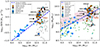 |
Fig. 3. Main scaling properties of the simulated galaxy samples compared to various observational datasets. Left panel: SFR vs M⋆ for MHONGOOSE (dB24, blue squares), J0342-47 (light blue hexagon), HALOGAS (Heald et al. 2011; Kamphuis et al. 2022, cyan diamonds), and our TNG50 (orange circles) and FIRE-2 (dark red stars) samples. The blue dashed line shows the SDSS main sequence from Chang et al. (2015). The grey circles show the other systems from the MW/M31 TNG50 sample of Pillepich et al. (2024). Right panel: MHI vs M⋆. The markers are as in the left panel, with the addition of the SPARC sample (Lelli et al. 2016, green triangles). The purple-shaded area shows the ±1σ confidence region around the median scaling found by Maddox et al. (2015), while the blue dashed line shows the linear fit to the H I-WISE data from Parkash et al. (2018). Masses for the simulated galaxies are computed within 100 kpc from their centre. Black-edged markers are used for systems that are studied in this work. For comparison, we also show the simulated galaxies with H I masses computed with the recipe of Gnedin & Kravtsov (2011) (empty stars and circles). |
2.3. Building synthetic H I observations
The realisation of synthetic H I datacubes from hydrodynamical simulations of galaxy formation has been pursued in a number of previous studies (e.g. Marasco et al. 2015; Oman et al. 2019). The procedure to build H I mocks is conceptually simple, but details may vary depending on the type of simulation adopted and on the specific goals of the mocks, which is why we describe it in some detail in this Section.
Here, mock H I datacubes were produced via a custom PYTHON software package and mimic the properties (FOV, spatial and spectral resolution, rms noise) of the MeerKAT observations. We had preferred to build our own routines rather than adopting already existing software (e.g. MARTINI, Oman 2019, 2024) in order to optimise the memory use and speed up the datacube construction on regular laptops. This approach was mandatory to process the computationally demanding FIRE-2 snapshots, and was adopted for TNG50 galaxies as well for consistency. For each simulated galaxy we produced two H I cubes, corresponding to the two different resolution sets discussed in Section 2.1 and whose main parameters are listed in Table 2. We considered all simulated galaxies as seen at a distance of 20 Mpc, similar to the typical distance of the five MeerKAT systems studied here (see Table 1). The volumes encompassed by the simulation snapshots are perfectly adequate to sample the entire FOV: TNG50 snapshots have a cubic shape with side-length of ∼800 kpc, FIRE-2 snapshots have a more irregular shape (because of the zoom-in nature of the suite) with a typical size of ≳1 Mpc and have zero contamination from low-resolution dark matter out to at least the virial radius (≃200 kpc).
In order to build the mock H I datacubes we needed to collect all gas particles within a snapshot that have non-zero H I mass and are within the cube boundaries defined in Table 1. The verification of the latter condition requires the knowledge of the galaxy centre, systemic velocity and projection on the plane of the sky. This information is easily accessible for the TNG50 cutouts from the MW/M31 sample, which have pre-computed spatial and velocity coordinates in a reference frame where the main galaxy is at the centre, and such that the z-direction is parallel to the stellar angular momentum vector (that is, the galaxy is seen as face-on in the xy plane). FIRE-2 snapshots do not provide this information. For these simulated data we determined the M⋆-weighted centroid using a series of spheres of progressively decreasing radius (starting from an initial radius of 1 Mpc), and then used all stars within 1 kpc from this position to determine the galaxy centre and systemic velocity. These were used for the computation of the stellar angular momentum vector (limited to the innermost 15 kpc region), which in turns set the galactic plane. The galaxy projection in the sky plane is regulated by two quantities: the disc inclination and position angle. For simplicity, in this study we adopted an inclination of 40°, similar to the mean inclination of the observed sample, and a position angle of 90° for all simulated galaxies. Matching the typical inclination of the observed galaxy population is particularly relevant for the study of the gas velocity dispersion, which can be affected by projection effects (e.g. Grisdale et al. 2017). Visual inspection of the stellar and H I maps confirmed that our projection routine works very well, especially when the stellar velocity field is clean and there are no close companions. The desired projection was achieved by applying appropriate rotation matrixes to all gas particles within the snapshot, before the application of the spatial and velocity cuts to match the FOV and velocity range of the observations.
The H I masses of the selected gas particles were distributed within the cube according to their projected coordinates (RA, DEC, vLOS). However, the H I mass of a given particle was not deposited entirely in a unique cube element, but it was smoothly distributed in a region of the position-velocity space. In the spatial domain, the size of such region depends on the intrinsic resolution of the simulation, while in the velocity domain it depends on the gas thermal broadening (see below for the details). If Mijk is the total H I mass contained within a given cube element with indexes (i, j, k), then the resulting flux density Fijk will be given by
 (2)
(2)
where Δv is the channel separation, D is the galaxy distance (assumed to be 20 Mpc), Bmaj and Bmin are sizes of the major and minor axes of the beam, and Δx and Δy are the pixel sizes.
In principle, the spatial resolution in the simulated data varies cell by cell, and can be taken as equal to ϵgas, the adaptive gravitational softening of a given gas cell (similar to the hydrodynamic smoothing kernel). However, employing a separate spatial smoothing for each gas particle in the cube is not only computationally challenging (as, for instance, up to 5 × 10⁶ particles must be processed for some FIRE-2 runs), but is also very inefficient: the FIRE-2 (TNG50) simulations studied here have minimum ϵgas of 1 pc (72 pc) whereas, for the adopted MeerKAT configurations, the spatial resolution in the mock data (ϵobs) is ∼2 kpc for the HR cube and ∼6 kpc for the LR one. As a significant fraction of gas particles will have ϵgas well below the resolution of the mock, we proceeded as follows. All particles with ϵgas < ϵobs were smoothed using the MeerKAT beam as a kernel, modelled as a 2D Gaussian distribution. The particles with ϵgas > ϵobs were partitioned into N = 7 different resolution bins, logarithmically spaced in size between ϵobs and the largest ϵgas available. Particles that belong to a given bin were smoothed using a constant Gaussian kernel with FWHM set to the median ϵobs of that bin. This ‘adaptive’ smoothing procedure is significantly faster than the ideal particle-by-particle treatment and produces very similar results. We had been experimenting with varying the number of resolution bins, finding no visible differences in the final (noisy) datacube for N > 5.
Similarly to Oman et al. (2019), thermal broadening was accounted for by assuming a constant velocity dispersion σth of 8 km s−1 for each gas particle, corresponding to a constant gas temperature of ∼8000 K, typical of the warm H I (McKee & Ostriker 1977). In practice, this was achieved by convolving the mock cubes in the velocity direction using a Gaussian kernel with a standard deviation of 8 km s−1. Our treatment for the thermal broadening is justified for TNG50, which does not resolve the cold atomic and molecular phases of the ISM and does not treat gas radiative cooling below a temperature of 104 K. For consistency we used the same approach also for the FIRE-2 runs, although in principle these would permit a more sophisticated treatment thanks to their superior ISM modelling and significantly lower (down to 10 K) temperature floor. However, we stress that individual H I line profiles in the resulting mock data are typically a factor ∼2 broader than the assumed σth (Section 4.5), which implies that the exact value adopted for this quantity has little impact on our results.
The procedure described above allowed us to produce noiseless H I datacubes with uniform sensitivity across the entire FoV. In order to transform these preliminary cubes into more realistic, MeerKAT-like mocks, two additional features were included. The first was the effect of the primary beam, which lowers the telescope sensitivity towards the periphery of the FoV. This was accounted for by multiplying each velocity channel by the median primary beam map5, which is available as part of the observational pipeline. The second feature was the injection of noise, which was done under the simplifying assumption that the noise is uncorrelated with the signal, in which case it was sufficient to produce a separate ‘noise-cube’ to be summed to the (primary-beam degraded) mock data. Under the assumption of a uniform, Gaussian noise (which holds up in MHONGOOSE data to a 4σ level, see Veronese et al. 2025), this noise-cube was produced starting from a temporary 3D array, having the same size of the data, made by values randomly extracted from a Gaussian distribution with zero mean and an arbitrary standard deviation. This temporary array was then convolved with the telescope beam6, re-normalised so that its resulting standard deviation was equal to that desired (that is, 0.15 mJy beam−1 for the HR and 0.25 mJy beam−1 for the LR), and finally summed to the mock data. We saved the original noiseless cubes and the final MeerKAT-like realisations separately, for future comparison.
3. Results
3.1. Detailed H I properties of a simulated galaxy
Before presenting a quantitative comparison between the simulated and the observed galaxies in a statistical manner, in this Section we discuss the detailed H I properties of a single simulated galaxy, system 543376 in TNG50. The goal is to provide a visualisation of the main differences between what the hydrodynamical simulation predicts and what could be determined with a putative H I observation with the MeerKAT telescope. Also, this exercise allows us to highlight the differences between the two resolution cases considered.
Fig. 4 shows a collection of diagnostic maps for 5433767. The top panels of Fig. 4 show properties that are predicted from the simulation but cannot be readily derived observationally, such as an H I column density map down to NHI of 1016 cm−2 (top left panel) and the H I-phase metallicity map with the vector velocity field overlaid on top (top right panel). These maps show that 543376 is characterised by an extended H I disc with a diameter of ∼60 kpc (measured at the H I column density level of 1020 cm−2), surrounded by a few extended H I filaments that connect the galaxy with the IGM, reaching the edge of the simulated FoV. The filaments are made of low-density H I (NHI ≲ 1019 cm−2) that streams towards the galactic disc, as can be seen from the 3D velocity field. The lack of clear stellar counterparts and the overall low metallicity indicate that the filaments are likely tracing cold gas accretion from the cosmic web, although part of the infalling gas may originate from re-accretion of material previously ejected from the disc by stellar feedback (recycling), especially the regions with higher metallicity (such as for the leftmost H I stream). It is not unusual for MW-like galaxies in cosmological hydrodynamical simulations to be embedded in multiple confluent filaments (e.g. Kereš et al. 2009; van de Voort et al. 2019), although this is not necessarily the case for all of the simulated systems considered in this work. We stress that the detailed H I morphology of this system is well resolved in the simulations. For instance, the entire top right filament is sampled by ∼104 gas particles with H I mass fraction > 10−5, and even the smallest isolated clump visible in the total H I map is sampled by at least a few tens particles.
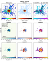 |
Fig. 4. Diagnostic maps of galaxy 543376 in the TNG50 simulation. Top row: H I column density map down to a depth of 1016 cm−2 (left), stellar surface density map overlaid with H I contours (middle), H I metallicity map overlaid with the vector velocity field (right). Central and bottom rows: Moment maps for the HR (central) and LR (bottom) mock H I data, derived with SoFiA. The main galaxy properties are listed in the leftmost panel of the central row. The iso-contours in the NHI maps are drawn at levels of 1016, 1017 (in grey, top panel alone), 1018 (in blue, top and bottom panels), 1019, 1020, 1020.5, and 1021 cm−2 (in black, all panels), with the iso-contour at 1020 cm−2 highlighted with a thicker line. In the moment-1 maps, the contour at the systemic velocity is shown by a black line, and consecutive contours are spaced by 25 km s−1. The beam sizes are shown as red ellipses in the bottom right corner of the moment-0 maps. The dashed grey iso-contours in the top left panel trace the surface density distribution of the dark matter halo. |
The panels in the central and bottom rows of Fig. 4 show the standard moment-0, moment-1 and moment-2 maps derived by processing the mock H I datacubes (which include noise) using the same methodology that was adopted for the MeerKAT galaxies, which is described in Section 2.1. As expected, the differences with respect to the ‘infinite-depth’ NHI map are striking, especially for the HR case (central row) where the H I filaments surrounding the galaxy disc are completely invisible. The increased sensitivity of the LR case permits instead to capture a few faint H I clouds located to the left of the galactic disc and, importantly, to marginally increase the size of the H I disc itself, emphasising the outer warp in the velocity field (moment-1 map), visible as a twist in the kinematic position angle. A possible interpretation for kinematic H I warps observed in real galaxies is that they originate from accretion events (e.g. Jiang & Binney 1999), which is likely the case here as well. We point out that the degraded resolution of the LR case prevents us to identify the filamentary H I structure that would be otherwise partially visible with a sensitivity of 1018 cm−2 at a higher resolution, as shown by the top left panel in Fig. 4.
Another relevant feature of the mock observations is the presence of localised, multiple high-velocity peaks in the moment-2 maps, visible as bright spots at velocity dispersion σ ≳ 50 km s−1 for both the HR and the LR cases. Such large values for σ are very rarely observed in MeerKAT galaxies (see Fig. 1), or in local star-forming galaxies (e.g. Tamburro et al. 2009; Bacchini et al. 2019). In general, high-σ peaks can originate from kinematically hotter components (i.e. highly turbulent H I regions), or can be caused by the overlap of multiple cold kinematic components along the line of sight. These two options are further discussed in Section 4.5, where we characterise the shape of the H I line profiles in our mock datacubes and compare it to the observations. Interestingly, for galaxy 543376, these high-σ peaks appear to be localised in regions where the H I filaments and the disc join each other (in projection), which would support a physical origin from the dissipation of gravitational energy of the accreting gas (e.g. Klessen & Hennebelle 2010; Krumholz et al. 2018). We verified that this is the case by visually inspecting a face-on projection of all individual H I-rich gas particles, confirming that particles at the intersection regions between the filaments and the disc show a significantly larger |vz| (the modulus of the velocity in the direction perpendicular to the disc) with respect to the surrounding gas. This experiment confirmed that projection effects do not play a major role. Visual inspection of the diagnostic maps of the other simulated galaxies revealed that the presence of high-σ regions is a common feature of TNG50 and FIRE-2 simulated galaxies. In Section 4.4, we discuss how the combined effects of feedback and accretion from the cosmic web play an important role in producing these features.
In the remaining part of the analysis we focus on a comparison with the observed sample in terms of moment-0 and moment-2 maps. The study of velocity fields is extremely interesting as it can potentially reveal key information on the properties of the accreting gas and of dark matter halos (e.g. Marasco et al. 2018; Oman et al. 2019; Sharma et al. 2022; Roper et al. 2023), but it requires a dedicated analysis which we plan to present in a future contribution.
3.2. Column density and velocity dispersion distributions
We now compare the observed H I properties of the three galaxy samples studied in this work. To do so, we rely on two-dimensional density histograms of the zeroth and second moment values, which we computed for all galaxies combined in a given sample, using only pixels within the masks provided by SoFiA. It is worth stressing again that the masks were constructed in an identical manner for all three samples. The 2D distributions are shown in Fig. 5, with a separate panel for each sample and resolution mode, and are produced using bins of 0.2 dex in NHI and 0.05 dex in σ. To account for projection effects, the column density inferred from moment-0 maps were corrected for galaxy inclination, which we take from Table 1 of dB24 for the MHONGOOSE galaxies, from Stuber et al. (2023) for J0342-47, and is fixed at 40° for the simulated samples.
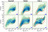 |
Fig. 5. Two-dimensional density histograms of the inclination-corrected H I column density and second moment values for MeerKAT (left panels), TNG50 (central panels), and FIRE-2 (right panels) galaxies. The top and bottom panels show the HR and LR cases, respectively. The black contours encompass 25%, 50%, 75%, and 95% of the highest density gas of the integrated distribution. The red dashed contours in the TNG50 and FIRE-2 panels reproduce the outermost contour of the MeerKAT distribution, and are included as a reference. |
In our observed sample, the 2D distribution resembles that presented in dB24, though with slightly lower S/N due to the smaller number of galaxies analysed here. We clearly see a well-defined peak at NHI ≃ 5 × 1020 cm−2 and σ ≃ 15 km s−1 for both resolution cases. The typical σ stays constant down to NHI values in the range of 1019–1020 cm−2 (the exact value depends on the resolution), and below 1019 cm−2 the two quantities appear to be strongly correlated. As extensively discussed in section 7.3 of dB24, this correlation is artificial, and is caused by the limited sensitivity: low signal-to-noise H I lines will have their high-velocity wings clipped out by the SoFiA mask, which will diminish the measured line width in a way that depends on the strength of the signal. This also explains why σ stays flat down to column densities that are lower in the LR mode.
Although similar in its overall shape, the 2D distribution determined for the simulated galaxies shows important differences with respect to the MeerKAT sample. First, both TNG50 and FIRE-2 galaxies show at least two separate peaks, one typically associated with low values of NHI and σ, the other associated with higher densities and line-widths. This bimodality is particularly evident in TNG50 galaxies for the LR mode, but it is present also in the other simulated samples. We verified that the bimodality is present regardless of the recipe adopted to separate molecular from atomic hydrogen, thus we can consider it as a systematic feature of the hydrodynamical models analysed here. In MeerKAT, the bimodality is not visible in the HR cubes. A very weak secondary peak is visible in the LR cubes at NHI ∼ 1019 cm−2 (as also noticed by dB24), but this is much fainter than that in the simulated galaxy sample, and shifted to a factor ∼10 higher column density. A consequence of this discrepancy is that the simulated galaxies show an excess of low-NHI material, as we discuss further below. A second difference that can be appreciated from the panels in Fig. 5 is that the simulated galaxies feature a more pronounced extension to high-σ values than the observed systems. We already mentioned this feature when discussing the detailed H I properties of 543376 in Section 3.1. Here, we notice that the high-σ H I in the simulated galaxies is present at all column densities, but it is more visible at 1019 < NHI < 1020 cm−2 in TNG50 and at NHI > 1020.5 cm−2 in FIRE-2. This suggests that the high-σ regions are more concentrated within the densest, star-forming regions of FIRE-2 galaxies, whereas they are distributed at the periphery of the discs of TNG50 galaxies, as we discussed for 543376. At a column density of ∼1020 cm−2, we observe a bifurcation in the velocity dispersion of FIRE-2 galaxies, which can be linked to the multiple components present in these simulations, as discussed later in the paper (Section 4.5). This bifurcation appears in the LR plot but is less visible in the HR plot.
Fig. 6 shows the probability density function (pdf) of the inclination-corrected NHI and second moment (σ) values, averaged over all galaxies in a given sample, for the three samples and the two resolutions considered. Specifically, for a given sample, the median pdf is shown as a solid line, while galaxy-to-galaxy fluctuations are represented as shaded regions and are computed as the difference between the 84th and 16th percentile of the ensemble of pdfs. Fig. 6 better highlights the differences between the observed and simulated systems. The NHI distributions of the MeerKAT galaxies and of the simulated ones have a markedly different shape, indicating that, on spatial scales of a few kpc, there is an intrinsic difference between the observations and the simulations in the distribution of H I inside and around local star-forming galaxies. In particular, both the TNG50 and the FIRE-2 systems show an excess of H I at column densities ≲1020 cm−2, which we further investigate in Section 3.3. FIRE-2 systems also show an excess of H I at NHI > 1021 cm−2. Such high NHI values are rarely observed in real galaxies, and in the simulations are largely dependent on the atomic-to-molecular partition recipe adopted. They would disappear if we used a recipe different from that of Blitz & Rosolowsky (2006). This is shown in Fig. A.3 for the recipe of Gnedin & Kravtsov (2011), but the recipe of Krumholz (2013) gives comparable results. We remark though that the Blitz & Rosolowsky (2006) recipe is the one that better reproduces the observed molecular gas fraction in galaxies, at least in the mass range considered in this study, as shown in Fig. 2. The right panel of Fig. 6 shows that the differences in the σ distribution are significant. First, with respect to the observations, the simulations show a more pronounced tail towards large σ values. To provide a reference, it is two (four) times more likely to find a pixel with σ of ∼40 km s−1 in the moment-2 maps of TNG50 (FIRE-2) galaxies than in the real ones. Additionally, while the σ distributions in the MeerKAT sample and the TNG50 sample are unimodal and peak at approximately the same value (∼15 km s−1), FIRE-2 galaxies feature a bimodal distribution with separate peaks at ∼12 km s−1 and ∼30 km s−1. As shown in Fig. 5, these two σ peaks correspond to different NHI regimes, with the high-density and low-density H I showing distinct kinematics. The comparison presented here highlights how the differences between the observed and simulated galaxy samples are not negligible, especially in the case of FIRE-2.
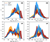 |
Fig. 6. Probability density distribution of inclination-corrected NHI values (left panels) and second moment values (right panels) for MeerKAT (blue), TNG50 (orange), and FIRE-2 (dark red curves) galaxies. The HR and LR cases are shown in the top and bottom panels, respectively. The solid lines show the median distribution for a given galaxy sample, while the shaded regions show the scatter within the sample, computed as the difference between the 84th and 16th percentiles. |
3.3. H I spatial distribution
While Section 3.2 focused on the overall column density and velocity dispersion distribution for the ensemble of galaxies in a given sample, we now address the question of whether individual TNG50 and FIRE-2 systems show any relevant differences with respect to the observed galaxies in terms of spatial distribution of their H I content.
Figure 7 shows the cumulative H I profiles (normalised to one) as a function of the projected distance from the galactic centre for each galaxy in our samples. We show the profiles for the HR case, but the LR case is very similar. To avoid abrupt discontinuities caused by the presence of isolated H I-rich satellites, we assumed that a profile has reached its asymptotic value if there exists a window with a size of at least 20 kpc where it shows no growth. In practice, each profile was inspected for the presence of a flat region with a length of at least 20 kpc and, if such a region was identified, the remaining part of the profile at larger radii was discarded. This approach allowed us to trace the distribution of H I that is spatially connected with the main galaxy, ideally avoiding to sample external galaxies that may be dynamically unrelated with the observed target.
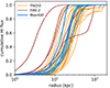 |
Fig. 7. Cumulative H I flux as a function of the projected distance from the galaxy centre for individual MeerKAT (blue), TNG50 (orange), and FIRE-2 (dark red) systems (HR case). Abrupt discontinuities due to the presence of isolated H I-rich satellites have been removed from all profiles. |
Fig. 7 indicates that FIRE-2 galaxies are typically too concentrated compared to the TNG50 and the observed systems. On the contrary, several TNG50 systems are less concentrated than the observed galaxies as they often show central H I holes (visible in Fig. 9) related to the ejective character of SMBH feedback, as discussed in Gebek et al. (2023). While we refer to Diemer et al. (2019) and Gensior et al. (2024) for a detailed investigation of the H I mass-size relation in MW-like galaxies from hydrodynamical simulations, it certainly appears that, at least for the samples considered in our study, there is a large discrepancy between FIRE-2 and TNG50 in the predicted sizes of H I discs at fixed H I mass. In addition, most TNG50 systems have a significant fraction of H I distributed at large distances (50 − 150 kpc) from the galactic centre. In particular, the percentage of H I flux located beyond a projected distance of 70 kpc from the galaxy centre is always < 1% for all systems in the MHONGOOSE sample, while it can reach up to 14% in the TNG50 sample and 32% in one FIRE-2 galaxy (m12r). This result does not depend strongly on the length of the window used to filter out H I-rich satellites, and indicates a general mismatch in the way the cold gas is spatially distributed in the simulated galaxies and in the observed ones.
The fact that several systems feature too much H I in their outskirts is not due to the presence of a collection of high-density clumps at large galactocentric distances, but rather to an excess of low-NHI material surrounding the galaxy discs. This can be appreciated by looking at the diagnostic maps in Appendix A, and is quantified in Fig. 8, which shows how the fraction of spaxels at NHI < 1020 cm−2 (computed with respect to all spaxels available within the SoFiA mask, without any filtering) is distributed amongst the different galaxy samples, for the LR case which is the most sensitive to low-NHI features. The percentage of low-NHI spaxels is in the range 45 − 65% for all MeerKAT galaxies. Most galaxies in the simulated sample have values higher than the highest MeerKAT value: two FIRE-2 and 15 TNG50 galaxies show values between 65% and 85%. A similar result can be derived for the HR mode, but with a marginally less clean separation between the observed and simulated samples due to the lower NHI sensitivity, which prevents the identification of the faintest H I features in the outskirts of the simulated galaxies. We stress that, as shown by Veronese et al. (2025), the stacking of MHONGOOSE data suggests the absence of additional H I signal in the galaxy halos down to column densities of ∼1017 cm−2.
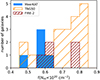 |
Fig. 8. Distribution of the fraction of spaxels with H I column densities below 1020 cm−2 for the LR cubes in MeerKAT (filled blue histogram), TNG50 (hatched orange histogram), and FIRE-2 (hatched dark red histogram). The fraction is computed with respect to all spaxels that contribute to the moment maps. |
3.4. Regular and irregular H I discs
The separation visible in the histograms of Fig. 8 allows us to split galaxies in our samples into two categories, above and below f(NHI < 1020 cm−2) values of 0.65. The total H I maps of galaxies belonging to each category are collected in Fig. 9 for the HR case, and appear quite different. Galaxies with f < 0.65 generally show a regular morphology characterised by well-defined discs, possibly surrounded by a small number of H I-rich satellites. All MeerKAT galaxies (highlighted with green boxes in Fig. 9) fall in this category. Galaxies with larger f values show more irregular morphologies, featuring filamentary or uneven H I envelopes which suggest a more complex interplay with their environment. Moment-1 and moment-2 maps for the two categories are shown in Appendix A. A visual inspection of these maps indicates that, qualitatively, the simulated galaxies that belong to the regular category (especially those from the TNG50 sample) are very similar to the observed galaxies in their morphology and kinematics. We explore this more quantitatively in Fig. 10, where we present again the NHI and σ distributions shown in Fig. 6 for the HR case, but for the regular and irregular simulated systems separately. Interestingly, in TNG50, although regular galaxies make up to only one fourth of the simulated sample, their typical NHI and σ distributions are in excellent agreement with the observations. This is not the case for the irregular TNG50 galaxies, or for FIRE-2 galaxies in general. Insights on the physical origin of the difference between the regular and irregular populations are provided below, and in particular in Section 4.3.
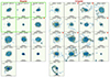 |
Fig. 9. Moment-0 maps for all galaxies in our sample divided into regular (on the left) and irregular (on the right), depending on whether the fraction f of spaxels with H I column density below 1020 cm−2 is higher or lower than 0.65 (see Fig. 8). f values of individual galaxies are annotated in each panel. The red dots mark TNG50 galaxies that have AGN feedback in thermal mode. The black iso-contours from the HR maps are drawn at levels of 1019, 1020 (thicker line), 1020.5, and 1021 cm−2. An additional iso-contour from the LR maps at 1018 cm−2 is shown in blue. The green boxes highlight galaxies observed with MeerKAT. The maps were derived with SoFia-2, using the same parameters for all galaxies. |
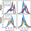 |
Fig. 10. As in Fig. 6 for the HR case, but with the simulated galaxies split into regulars (top panels) and irregulars (bottom panels). Regular TNG50 galaxies follow the distributions observed with MeerKAT very well. |
4. Discussion
In this Section we focus preferentially on the simulated galaxies and discuss how some of their properties (environment, star formation rates, gas accretion rates) play a role in shaping their H I distribution and kinematics. We also attempt to quantify the complexity of their H I profiles in more detail, in order to provide more insightful comparison with the data.
4.1. Gas inflows and outflows
One of the great advantages of hydrodynamical simulations of galaxy formation and evolution is that the three-dimensional gas flow can be traced at any distance from the galaxy centre, regardless of the gas temperature, density and ionisation state. Accurate measurements for the gas inflow and outflow rates are very difficult to obtain observationally (e.g. Sancisi et al. 2008; Di Teodoro & Peek 2021; Kamphuis et al. 2022; Marasco et al. 2023) due to a combination of projection effects and the impossibility of sampling all gas phases simultaneously in a homogeneous way, with sufficiently high spatial and spectral resolution.
To investigate the instantaneous gas flow in the simulated galaxies, we divided each snapshot into a series of spherical shells, all centred at the galactic centre and with variable thickness. In each shell, we computed the mass-weighted radial speed ⟨vr⟩ and the net flow rate Ṁ, which are defined as
 (3)
(3)
 (4)
(4)
where the sum is extended to all N gas particles in the shell, vr, n is the particle radial speed, mn is the particle mass, wn is a weight that depends on which gas phase is being considered (it is equal to the gas particle H I fraction if we focus on the H I, or to one if we consider all phases together), and Δr is the shell thickness. For TNG50 we also included the so-called wind particles (see Pillepich et al. 2018) assuming that they are made of fully ionised gas, finding that their contribution to the flow rate is negligible for the galaxies studied here. Equation (3) gives the typical speed at which the gas is flowing into (or out from) the shell considered, while Equation (4) provides the instantaneous mass flow rate in a shell. Both equations can be applied to the inflowing (vr, n < 0) and outflowing (vr, n > 0) gas particles separately in order to study the inward and outward motions independently, or to all particles (regardless of the sign of their vr, n) to infer the properties of the ‘net’ gas flow. By averaging the inward and outward flows, the net flow indicates whether the gas in a given shell is moving on average in one direction or the other. We remark that, as in our calculations we accounted for all gas particles available in the snapshot, at small radii (r < 10 − 20 kpc) the flow will be dominated by motions within the galaxy disc.
Fig. 11 provides the radial profiles of ⟨vr⟩ (top panels) and Ṁ (bottom panels) for the inflowing and outflowing components separately (leftmost panels), for the net flow of all gas phases (central panels) and for the net flow of the H I phase alone (rightmost panels). Individual galaxies show a substantial scatter in their radial profiles; thus we focus on the median profiles computed (shell by shell) using all galaxies in the TNG50 and FIRE-2 samples separately, which are represented by the thick lines in Fig. 11. The leftmost panels of Fig. 11 show that, at all radii, the gas moves inwards and outwards with velocities ranging from a few tens up to ∼100 km s−1 (panel a), leading to flow rates up to a few tens M⊙ yr−1 in both directions (panel d). Our interpretation for the remarkable symmetry shown by the inflow and outflow rate profiles is that gas in the halo moves inwards following slightly eccentric orbits, possibly caused by a triaxial gravitational potential, thus measurements via Equation (4) that assumes a spherical symmetry will infer large inward and outward rates due to the gas radially oscillating along its non-circular orbits. We verified that the percentage of gas mass that flows in the tangential direction (as opposite to the gas that flows radially) is always > 50% at all radii, which validates our interpretation. We postpone a detailed investigation of the 3D kinematics of gas in the simulations to a future study, together with the analysis of the mock velocity fields. However, the considerations above exclude a 100 kpc-scale galactic fountain as the origin of the flows shown in panels (a) and (d) of Fig. 11.
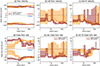 |
Fig. 11. Radial velocities (top panels) and gas mass flow rates (bottom panels) computed in spherical concentric shells, as a function of the shell radius, for the TNG50 (orange) and FIRE-2 (dark red) galaxies. Panels (a) and (d) show the inflow and outflow components separately, panels (b) and (e) show the net (outflow-inflow) flow for all gas phases, panels (c) and (f) show the net flow for the H I alone. The thick lines show the median trend, while the shaded areas show the difference between the 84th and 16th percentile. Negative values indicate inflow. |
For the reasons discussed above, the net flow is likely a more robust quantity to study for our purpose. The central and rightmost panels of Fig. 11 focus on the net flow and show that, in general, there is a tendency for the gas to flow inwards at all radii. Focussing on the H I, the radial speed of this inward flow is very similar for the two simulation suites (panel c). The small amount of H I located at the virial radius r200 (≃200 kpc for the systems studied here) flows in with speeds of ∼50 − 100 km s−1; this velocity decreases progressively as the gas interacts with the pre-existing CGM, down to about 10 km s−1 at r ≃ 10 − 30 kpc as the material joins the H I disc and proceeds inwards. However, the median profiles for the H I accretion rates in TNG50 and FIRE-2 galaxies (panel f) are quite different, due to the substantially diverse density profiles predicted by the two suites. FIRE-2 galaxies feature an H I mass accretion rate of a few M⊙ yr−1 in all shells with r < 20 kpc, down to the galaxy centre. The total gas mass accretion rate (panel e) in these regions is about twice that provided by H I alone, and with values between 2 and 10 M⊙ yr−1 it closely matches the range of SFRs of FIRE-2 galaxies (Table 3), supporting a connection between gas accretion and star formation processes. The accretion proceeds steadily also at r > 20 kpc, although it is not traced any longer by the H I phase. In TNG50 galaxies, instead, ṀHI peaks at 30 − 40 kpc from the galactic centre, which is approximately the region where the inflowing filaments join the disc in the example galaxy discussed in Section 3.1, and decreases drastically in the innermost regions of the disc. Considering that the inflow speeds are very similar (panel c), this discrepancy is caused by the different density profiles in the TNG50 and FIRE-2 systems, with the latter featuring a much more concentrated gas distribution than the former, likely caused by the lack of AGN feedback in FIRE-2. The H I accretion rate profiles are somewhat sensitive to the H I-to-H2 partition scheme: the GK11 recipe leads to a factor ∼2 lower H I flow rate in TNG50 galaxies, and an almost null H I accretion in the innermost 4 kpc of FIRE-2 galaxies. However, the discrepancy between the two simulation suites is visible also in the accretion profiles of the total gas content (panel e), which strengthens our interpretation of the gas flow.
Fig. 12 shows the net mass flow rate for gas with metallicity < 0.5 Z⊙. As expected, the gas that flows in from the outer regions of the halo has a low metal content, but it gets progressively polluted as it approaches the disc. We notice that the Ṁ profile for the low-Z gas and the ṀHI profile shown in panel (f) of Fig. (11) are complementary (one increases where the other decreases), which can be due to the pollution promoting the cooling of the inflowing gas with subsequent increase of its H I fraction, a physical process that has been explored in the literature using wind-tunnel simulations at pc-scale resolution (Marinacci et al. 2010; Armillotta et al. 2017). Another possibility, which may coexist with the previous one, is that high-Z H I in the disc is dragged inwards by the accreting flow of low-Z ionised gas from the CGM. For a more in-depth investigation of gas flows in MW-like galaxies in the FIRE-2 simulations we refer to Trapp et al. (2022).
The comparison of panels (e) and (f) of Fig. 11 shows that, in regions sufficiently close to the H I disc (r ≲ 30 − 50 kpc), the ṀHI and the Ṁ profiles are similar (especially in TNG50 galaxies), indicating that the H I is a good tracer of gas inflows. If correct, this prediction supports the idea that deep H I observations, such as those provided by the MHONGOOSE survey, are key to provide insight into the process of gas accretion onto galaxy discs. However, the accretion picture shown by the simulations studied here appears to be in tension with recent determination of the distribution of the extraplanar warm (∼104 − 105 K) gas around the Milky Way, where virtually all gas traced by H I and metal low-ions is confined within a height of ≃10 kpc from the disc (Lehner et al. 2022; Choi et al. 2024) and is formed, in most parts, by gas participating in the galactic fountain cycle (Marasco et al. 2022). In other words, there is no observational evidence for gas accretion onto the Milky Way from T ≲ 105 K clouds located at several tens of kpc from the disc. Assessing the magnitude and the implications of such tension would require a dedicated analysis which goes beyond the scope of this work.
4.2. Environment
One may wonder whether the differences between the observed and the simulated galaxy samples can be caused by differences in the local environment. MHONGOOSE galaxies are in fact specifically selected to be either isolated or to belong to the outer regions of small groups (dB24). Target galaxies in the TNG50 MW/M31-like sample, for instance, have no companion with M⋆ > 1010.5 M⊙ at distances < 500 kpc by construction, but lower mass companions can be present and may have an impact on the H I distribution and kinematics of the main galaxy.
We had characterised the local environment of each galaxy in the TNG50 and the observed samples by determining the number Nenv of satellites with M⋆ > 107.5 M⊙ and MHI > 107 M⊙ within 250 kpc of projected distance and ±500 km s−1 of line-of-sight velocity from the main galaxy. For the simulations we analysed the TNG50 sample alone because, unlike FIRE-2, the associated satellite catalogue stores information on the H I content of each subhalo, which was needed for our analysis. We stress that Nenv can be determined in an identical manner in both observations and simulations, with the caveat that satellite stellar masses in the observed sample are determined from gri photometry from the DR10 of the Dark Energy Camera Legacy Survey (DECaLS; Dey et al. 2019), where the apparent magnitudes were converted to M⋆ assuming the distances of the central galaxies, and using the relations given in Taylor et al. (2011).
We limited the count of satellites to those having non-negligible H I content because this was how companion galaxies were identified in the data. An advantage is that their line-of-sight velocity relative to the main galaxy can be measured, without requiring spectroscopic redshift measurements from other facilities. Given that the lowest H I mass companion presented in dB24 is ∼107 M⊙ (see their Fig. 16), we determined Nenv in TNG50 using this H I mass threshold, which implies that the H I content of the satellite was sampled with at least 100 gas particles. We notice that relaxing the requirement on the H I content has a strong impact on our results as, in our TNG50 sample, there are more satellites with MHI below the requested threshold than above.
We show the distribution of Nenv for the two samples in Fig. 13. There is a substantial difference in the typical environment of the two samples: 14 out of 20 TNG50 galaxies have no associated satellite with the properties requested, and only the remaining six appear to have Nenv compatible with the observations (Nenv = 2 − 3, with the exception of J0342-47 that has Nenv = 0). In Fig. 13 we also split the TNG50 sample in two subsamples, regular (densely hatched histogram) and irregular (sparsely hatched histogram), on the basis of the H I morphological classification of Fig. 9. Interestingly, all simulated galaxies with Nenv > 1 fall in the irregular category, which suggests the existence of a correlation between the presence of nearby companions and that of H I filaments and irregular H I envelopes surrounding galaxy discs.
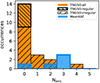 |
Fig. 13. Distribution of the local environment estimator Nenv, defined as the number of companions with M⋆ > 107.5 M⊙ and MHI > 107 M⊙ detected within 250 kpc of projected distance and ±500 km s−1 of line-of-sight velocity from the main galaxy, for the MeerKAT (blue histogram) and the TNG50 (orange histogram) galaxy samples. The densely and sparsely hatched histograms show the regular and irregular TNG50 populations, respectively (see Fig. 9). |
However, the correlation between satellites and H I features in the galaxy outskirts does not necessarily imply a causal connection between the two. In fact, the presence of companions may be caused by an overall more intense accretion flow from the cosmic web, which brings in both satellites and fresh gas from the intergalactic medium (IGM). We explore this scenario in Fig. 14, where we show the mean mass accretion rate of Z < 0.5 Z⊙ gas, averaged over 150 < r < 250 kpc (that is, around the virial radius r200), as a function of Nenv. The positive correlation between the two quantities indicates that environments with a larger number of satellites, which are those hosting central galaxies with a more irregular H I morphology (Fig. 13), accrete low-Z gas from the IGM at a faster rate. This correlation is maintained if we focus on the total accreted gas, rather than on the low-Z component alone.
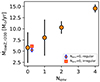 |
Fig. 14. Mass accretion rate of metal-poor gas (Z < 0.5 Z⊙), computed around r = r200 ≃ 200 kpc, as a function of the environment estimator Nenv, for TNG50 galaxies. The error bars account for the combined effect of galaxy-to-galaxy scatter and radial fluctuations in the Ṁ estimate around r200 in individual systems. The diamond and square markers show, respectively, the regular and irregular galaxies with Nenv = 0. Galaxies with more satellites show larger accretion rates. |
Finally, we remark that the number of low-M⋆ companions predicted by the simulations depends not only on the accuracy of the model in treating the environment physics, but also on the resulting galaxy stellar mass function. In contrast with other simulation suites (including the larger-volume runs from the IllustrisTNG project) which work on larger volumes and are calibrated to reproduce the statistics of the overall galaxy population, TNG50 is not tuned to output the observed galaxy statistics by construction. Although this does not imply that the resulting satellite statistics are incorrect, caution must be taken when generalising the results presented here.
4.3. What drives the difference between the regular and the irregular populations?
An important question to address is what is the primary physical mechanism that drives the irregularities in the H I morphology and kinematics of the simulated galaxies. We had checked that there are no major differences in the M⋆, M200 or SFR distribution between the regular and irregular galaxies, indicating that total dynamical mass or stellar feedback do not drive the difference between the two populations. Based on the analysis of Section 4.2, we can certainly assert that – at least in TNG50 – the environment is one of the factors that regulate the presence of low-NHI features at the periphery of galaxy discs, which is frequent in the simulated systems but is not visible in the observed ones: higher mass accretion from the cosmic web is typically associated with more companions that stream inwards with the accretion flow, producing a diffuse gas component around the galaxy which is expected to be observed with deep H I observations.
To verify that higher accretion rates onto halos correspond to stronger gas inflows onto galaxy discs (which may not necessarily be the case, see van de Voort et al. 2011), we had inspected the radial profiles of the net H I flow (see panel e in Fig. 11) for the regular and irregular TNG50 systems separately. We found a peak accretion value at 20 < R < 30 kpc of ∼2.5 M⊙ yr−1 for the former and of ∼5 M⊙ yr−1 for the latter. FIRE-2 galaxies behave similarly, although the largest difference in accretion rates between the regular and irregular systems is visible at R < 3 kpc, where we inferred ∼3 M⊙ yr−1 for the former and ∼10 M⊙ yr−1 for the latter. This confirms that the large-scale environment has an impact on the gas accretion onto galaxies, at least in the simulations studied here. We notice that the TNG50 irregular population hosts a higher fraction of systems in the so-called thermal AGN-feedback mode (6/15, compared to 1/5 for the regular ones). This is a direct consequence of the AGN feedback implementation scheme as these galaxies host SMBHs with masses just below 108 M⊙, a threshold where the z = 0 SMBH population has a clear change in accretion rate (Weinberger et al. 2017). These systems, marked by a red dot in Fig. 9, do not seem to have a distinct morphology or kinematics.
We believe that the fact that the observed galaxies feature regular and smooth H I discs with little diffuse low-NHI gas, even though they inhabit environments that are typically richer than those of most simulated galaxies (Fig. 13), indicates that a different, gentler, disc-halo interplay is at work in the observed Universe. More specifically, the processes of inflows and outflows that regulate the evolution of nearby late-type galaxies occurs without significantly disturbing the morphology and kinematics of H I discs, which is something that the simulations analysed here struggle to achieve. A similar conclusion was reached by Marasco et al. (2023) by studying the galactic wind properties in a sample of 19 nearby low-M⋆ starbursts. The fact that both regularly star-forming galaxies and starburst systems feature similarly mild gas flows around their discs is indicative of an overall gas circulation in nearby galaxies that is gentler than that predicted by the simulations. In this context, the galactic fountain framework proposed by Fraternali (2017), where the mild gas circulation produced by stellar feedback drives the cooling of the lower layers of the corona, seems to be a very promising model to interpret the observations.
4.4. The relation between moment-2 and stellar feedback
In Sections 3.1 and 3.2 we showed that simulated galaxies feature several high-velocity peaks in their moment-2 maps, which lead to a high-velocity tail in the σ distribution that is not present in the observations (right panel of Fig. 6).
There are various possible origins for the high-σ H I regions. Deep gravitational potential wells caused by massive bulges can promote turbulence within the ISM due to the increased shear in the innermost regions (e.g. Martig et al. 2009), but this effect is typically limited to the central kpc (Gensior et al. 2020) thus cannot be resolved by our mock H I data, not even for the HR case. A more promising option is that these features are due to the effect of stellar feedback, which injects both momentum and thermal energy into the gas surrounding star-forming regions8, leading to galaxy-scale winds and enhancing the velocity dispersion in localised regions of the disc. We tested this scenario in Fig. 15, which shows histograms of the local SFR surface density (ΣSFR) in TNG50 and FIRE-2 galaxies, divided into bins of different σ as determined from the moment-2 HR maps. The ΣSFR was extracted from maps that were built using gas particle-based SFRs, assuming the same observational properties (resolution, field of view, galaxy inclination and position angle) adopted for generating the synthetic H I HR data.
 |
Fig. 15. SFR surface density distribution in TNG50 (orange filled histograms) and FIRE-2 (dark red histograms) galaxies, for the HR case. Each panel accounts for spaxels in a given range of H I velocity dispersion, indicated at the top. |
Fig. 15 shows a clear distinction between FIRE-2 and TNG50 galaxies. In FIRE-2, the peak of the ΣSFR distribution shifts towards progressively higher values for larger σ bins, strongly supporting a stellar feedback origin for the high-σ H I regions. TNG50 galaxies show a more complex behaviour: the ΣSFR distribution peaks always at a similar value (∼10−3 M⊙ yr−1 kpc−1) but becomes wider as σ increases, with the exception of the highest σ bin (rightmost panel of Fig. 15). This suggests that, in TNG galaxies, star formation is not the primary driver of the high-σ H I features. Projection effects, accretion of pristine gas from the cosmic web, gas recycling, tidal interactions or wet minor mergers can all be responsible for a high-σ component that is uncorrelated with the ΣSFR.
In Section 3.1 we discussed a case where high-σ peaks appear to be located at the intersection between the H I disc and the surrounding filaments, supporting the existence of a causal connection between gas inflow and velocity dispersion enhancement. The inspection of the moment-2 maps shown in Figure A.2 reveals that there is a difference in the spatial distribution of the velocity dispersion between the two simulated samples: TNG50 systems exhibit multiple σ peaks, several of which are located in the outer regions of the discs, while FIRE-2 galaxies show more axisymmetric moment-2 maps, with the highest values that are systematically concentrated in the innermost regions of their discs. While the maximum moment-2 values in FIRE-2 galaxies can be found at the galactic centre and are due to beam-smearing, σ typically remains above 40 km s−1 up to ∼70″ from the centre (i.e. a distance much larger than the spatial resolution of the HR case). The difference between the two simulations can be interpreted in the light of the different gas accretion profiles shown by the TNG50 and FIRE-2 galaxies (Section 4.1). In FIRE-2 galaxies, gas streams inwards from the virial radius down to the innermost kpc with an approximately constant rate (bottom left panel of Fig. 11). This promotes an intense star formation activity in the central region of the galaxy, producing the high moment-2 values observed. It is possible that the lack of AGN feedback in the FIRE-2 runs plays a crucial role in this process, as one would expect that part of the accretion flow feeds the central supermassive black hole, whose feedback would act as a regulator of the flow itself. In TNG50, the gas accretion rate becomes negligible at ∼20 kpc from the centre, presumably where the inflowing filaments join the H I disc. This promotes the onset of turbulence also in the outer regions of the galaxy where star formation is negligible, explaining the lack of trends between SFR density and velocity dispersion (Fig. 15). These considerations aside, it is also possible that the different behaviour of TNG50 and FIRE-2 galaxies stems from the different response of the H I to feedback from star formation, due to the different resolution and feedback implementation of the two simulation suites.
4.5. The complexity of the H I line profiles
We now attempt to characterise the typical shape of the H I line profiles in the simulated and the observed systems, with the goal of providing quantitative measurements for their complexity. This exercise is also useful to understand whether the higher moment-2 values observed in the mocks are due to the presence of multiple components along the line of sight, to broader individual H I components, or to a combination of these effects.
We first provide an example of the different kinematic complexity exhibited by three systems in our samples. Fig. 16 shows a series of position-velocity (pv) slices for the MHONGOOSE galaxy J0419-54 (top panels), the TNG50 galaxy 543376 (central panels), and the FIRE-2 galaxy m12f (bottom panels). In general the pv slices of the observed and simulated galaxies appear very similar, and are dominated by the presence of a large rotating disc with an approximately flat rotation curve. Both in the observations and in the mocks there are very few H I clouds that are kinematically detached from the main disc, and virtually none of these reside in the counter-rotating regions of the pv slices. These considerations further stress the degree of realism achieved by present-day hydrodynamical simulations of galaxy formation.
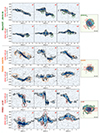 |
Fig. 16. H I position-velocity diagrams on slices parallel to the kinematic major and minor axes (first and second rows of each panel set) for J0419-54 (top panels), the TNG50 system 543376 (central panels), and the FIRE-2 system m12f (bottom panels) for the HR case. All panels show the same velocity range on the y-axis. The slice thickness is four pixels (20″). Slice offsets are indicated on the top right corner of each panel. Contours are spaced by powers of two, the outermost being at an intensity level of 0.3 mJy beam−1 (2σnoise). A negative contour (−2σnoise) is shown in grey. The circles highlight the anomalous kinematic features. The rightmost panels show the total H I maps with the cuts parallel to the major and minor axes (solid and dashed lines, respectively) used in the pv-slices. |
Upon closer inspection, Fig. 16 reveals two important differences between the MeerKAT observations and the mock data. First, the pv slices of J0419-54 are thinner (in the vertical direction) than those of the other galaxies, and especially than those of m12f. We verified that the thermal broadening adopted for the mocks (σth = 8 km s−1) is not the main source of the discrepancy, as models with σth = 5 km s−1 appear almost identical. To test whether the discrepancy arises from projection effects due to extremely thick discs in the simulations, which would smear the velocity profiles due to the line-of-sight intersecting layers at very different radii, we determined the H I scale-height radial profiles of the simulated galaxies by fitting their vertical H I distributions in different annuli with a Gaussian function (e.g. Olling 1995). The resulting scale-height profiles show clear signatures of inside-out flaring, with typical values of 0.5 − 1 kpc at R = 10 kpc, in line with the results of Gensior et al. (2023) for simulated MW-like galaxies from the FIREbox suite (Feldmann et al. 2023) and compatible with (or only marginally larger than) those inferred in nearby galaxies of similar M⋆ (e.g. O’Brien et al. 2010; Bacchini et al. 2019), including the Milky Way (Marasco et al. 2017). Thus we exclude that the thickness of H I discs plays a significative role in the cases studied here. The second difference is that the simulated galaxies show several H I features located at velocities that are anomalous with respect to those occupied by the bulk of the H I distribution at that specific location. Following a terminology that has often been adopted in the literature (e.g. Fraternali & Binney 2006; Sancisi et al. 2008; Gentile et al. 2013; Marasco et al. 2019), we refer to these features as extraplanar. These are highlighted with circles in Fig. 16, and are more prominent in the simulated galaxies than in J0419-54. This comparison already indicates that H I line profiles in TNG50 and (especially) FIRE-2 galaxies are individually broader and more complex than those in the observed systems.
In order to quantify the discrepancy between simulations and observations, we performed a multi-Gaussian decomposition of all line profiles within the SoFiA masks. Our approach consisted of fitting a variable number of Gaussian components, ranging from one to five, to all profiles whose peak signal-to-noise ratio is above two. The FIND_PEAKS subroutine of the SCIPY package (Virtanen et al. 2020) in PYTHON was used to identify the locations of multiple peaks, which, if detected, were used as first guess to the fitting procedure. Following Marasco et al. (2020) and Marasco et al. (2023), the optimal number of components was decided locally on the basis of a Kolgomorov-Smirnov (KS) test on the residuals of the fits determined using N and N + 1 components: if the two distributions of residuals were statistically different, the N + 1 component model was preferred. Thus, this method is sensitive to the relative improvements in the data fitting due to the use of increasingly complex model profiles, but it is independent of the goodness of the fit in absolute terms. A sensitivity threshold for the KS p-value must be adopted to reject the null hypothesis of identical residuals: this value ranges from zero (the test is insensitive to all variations in the residuals, hence only one component is needed) to one (the test is overly sensitive and all five components are always needed). Visual inspection of the resulting model profiles overlaid on top of the data indicated that a threshold very close to unity (1-ϵ, with ϵ = 5 × 10⁻⁵) is required in order to model the most complex line shapes.
We demonstrate our fitting procedure in Fig. 17, which presents a collection of five representative H I line profiles of the FIRE-2 galaxy m12f (HR), showing separately the mock spectra (in grey), the multi-Gaussian fits (in red) and the single Gaussian (in blue). All of these velocity profiles are well sampled by the simulation, as the number of gas particles with H I fraction > 10−5 that contribute to the H I lines ranges between a few thousands to a few tens of thousands. The various panels of Fig. 17 demonstrate that the multi-Gaussian model fits the mock data very well, using a variable number of components depending on the complexity of the line profile analysed. We notice that, even with the relatively large sensitivity threshold adopted, the approach taken prefers a limited number of components and does not overfit the mock. This is particularly visible in the fourth panel of Fig. 17, which gives the impression that the number of components adopted to model the simulated line profile (two) is somewhat conservative. This indicates that our method of decomposition likely provides a lower limit on the number of components.
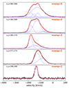 |
Fig. 17. Representative H I spectra for the FIRE-2 galaxy m12f (HR), extracted at the pixel positions indicated in the top left corner of each panel. The grey lines show the mock H I spectra, the red lines show the best-fit multi-Gaussian models, the blue lines show the individual Gaussian components. The number of components used is indicated in the top right corner of each panel. |
We used this approach to produce multi-Gaussian fits for all TNG50, FIRE-2 and MeerKAT systems. To compare our results amongst the three samples, we made use of two quantities. The first was the fraction of spectra modelled with a given number Ncomp of components. The second quantity was computed by building, using all spectra modelled with Ncomp components, the distribution of the Gaussian standard deviations associated with each component, and then extracting the median of such distribution. In practice, the first quantity accounts for possible differences in the typical number of H I components, whereas the second is informative of the typical broadening of the individual components. Both quantities were computed using only the unmasked spectra of all galaxies of a given sample, that is, using only the spectra that contribute to the various moment maps. The leftmost panels of Fig. 18 show how these two quantities vary as a function of the number of components in the three galaxy samples, and for the regular and irregular populations separately. Clearly, the origin of the discrepancy between the simulated and the observed galaxies is twofold: with respect to the mocks, the H I profiles in the real galaxies are characterised by a typically lower number of components, each having on average lower standard deviations. In particular, FIRE-2 galaxies are those that show the largest deviations from the observations, featuring a factor ∼2 more 5-component profiles than the MeerKAT galaxies, and a factor of ∼1.7 higher standard deviations at N = 5. As expected, the regular population provides a marginally better match to the data.
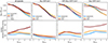 |
Fig. 18. Results of our multi-Gaussian fitting for the TNG50 (orange), FIRE-2 (dark red), and MeerKAT (blue) galaxies. Top panels: Fraction of spectra modelled with N components (1 ≤ N ≤ 5). Bottom panels: Median value of the distribution of the Gaussian standard deviations computed for all line profiles modelled with N components, as a function of N. The different panels show our results for spaxels in different ranges of (inclination-corrected) H I column density, indicated at the top of each panel. The dashed and dotted curves in the leftmost panels show, respectively, the regular and irregular populations of simulated galaxies. |
To identify whether the trends visible in the leftmost panels Fig. 18 depend on the H I column density, we repeated our analysis using only spaxels in given ranges of (inclination-corrected) NHI: below 1020 cm−2, between 1020 and 1020.5 cm−2, and above 1020.5 cm−2. These are shown in the second, third and fourth columns of Fig. 18. Unsurprisingly, we find a larger number of components and a stronger broadening for increasing values of NHI. Interestingly, the largest deviations between the mocks and the data are visible for the highest NHI bin in FIRE-2, and for the intermediate NHI bin for TNG50. This strengthens our idea that the peculiar kinematics of FIRE-2 galaxies is driven primarily by stellar feedback, which affects preferentially the high-NHI gas, whereas the high-σ regions in TNG50 galaxies are produced by a different mechanism such as accretion of cold gas filaments at the periphery of their disc, as discussed in Section 4.4.
We can robustly conclude that the simulated galaxies, and in particular those from the FIRE-2 suite, feature more complex and broader H I line profiles than the observed galaxies, and that such peculiar kinematics is caused by a more complex gas cycle within and around their discs.
5. Conclusions
The distribution and kinematics of gas in and around galaxy discs is influenced by internal and by external processes such as stellar and AGN feedback and gas accretion from the circumgalactic medium. These processes produce large-scale gas circulation whose impact is expected to be more visible in the low column density gas located at the interface region between the galactic disc and the halo. Deep observations are needed to probe gas in this region, and state-of-the-art galaxy evolution models are required for their interpretation.
In this study we used wide-field (1° ×1°), spatially resolved (down to 22″), high-sensitivity (∼1018 cm−2) H I observations with the MeerKAT radio telescope of a sample of five Milky Way-like galaxies. The typical galaxy distance of 20 Mpc allowed us to sample a region of a few hundred kiloparsecs around their disc with a spatial resolution of 2 − 6 kpc, depending on the angular resolution adopted. We compared these data with synthetic H I observations generated from a sample of 25 simulated star-forming galaxies from the TNG50 (20) and FIRE-2 (five) suites of cosmological hydrodynamical simulations in the ΛCDM framework. The simulated galaxies were selected to be similar to the observed galaxies in terms of stellar mass, SFR, and H I content, and the mock H I datacubes (and associated moment maps) were built using the same sensitivity, resolution, and field of view as the MeerKAT observations. This approach allowed us to process both observations and simulations with a similar methodology, limiting the bias in the comparison between the two. Our results can be summarised as follows:
-
By exploring different recipes (Blitz & Rosolowsky 2006; Gnedin & Kravtsov 2011; Krumholz 2013) for the atomic-to-molecular hydrogen partitioning in the simulations, we found that the Blitz & Rosolowsky (2006) approach leads to H2-to-H I mass ratios that are in good agreement with those inferred in the local Universe (Fig. 2). The other recipes overestimate the H2-to-H I mass ratio by up to an order of magnitude, and we advise against using them to infer H I and H2 masses in TNG50 and FIRE-2 galaxies.
-
Compared with the MeerKAT sample, the simulated galaxies show on average an excess of low column density gas (NHI < 1020 cm−2) in their outskirts (left panels of Fig. 6 and Fig. 8); several systems have 10 − 20% of their total H I content distributed at 50 − 150 kpc from their disc (Fig. 7).
-
While all galaxies in the observed sample appear as regular discs, the simulated galaxies frequently show disturbed and irregular H I morphologies. In particular, all systems whose H I spatial distribution is dominated by column densities < 1020 cm−2 show strong irregularities (Fig. 9).
-
The local environment plays a key role in shaping the H I distribution of simulated galaxies. H I-irregular systems inhabit halos with more satellites (Fig. 13) and with higher gas accretion rates (Fig. 14) than those hosting more regular H I discs. However, the observed galaxies always show regular H I discs in spite of hosting a number of H I-rich satellites typically larger than the satellites found near simulated systems.
-
The simulated galaxies show a high-velocity tail in their moment-2 distribution that is not visible in the real systems (right panels of Fig. 6). This tail is produced by line profiles that have, on average, a broader and overall more complex shape than those observed with MeerKAT (Figs. 16 and 18). These features are stronger in FIRE-2 than in TNG50.
The complex kinematics shown by the simulated galaxies is caused by the combined effect of extragalactic gas accretion and stellar feedback. In FIRE-2 galaxies, gas streams inwards from the virial radius down to the innermost kiloparsec at an approximately constant rate, promoting an intense star formation activity (Section 4.1) that leads to the high moment-2 values concentrated towards the central regions of the galaxy (Fig. A.2). In TNG50, the inward accretion flow stops at the disc periphery, promoting turbulence also in the outer regions of the galaxy where star formation is negligible. Real galaxies show quieter kinematics. Our results support a scenario where gas circulation caused by stellar feedback and accretion from the cosmic web in real galaxies is gentler than in the simulated galaxies. This leads to H I discs that are less turbulent, feature less diffuse low-NHI (< 1020 cm−2) emission, and overall show a more regular morphology than those in the cosmological hydrodynamical simulations considered here. A promising scenario that could explain the observed H I properties of nearby disc galaxies is that of the galactic fountain (Fraternali 2017).
In spite of their very different characteristics (hydro code, mass resolution, and subgrid physics), the TNG50 and the FIRE-2 simulations both show shortcomings when compared to the data. One may wonder whether the discrepancies between the simulated and the observed galaxies are due to some missing physics in the models (e.g. radiative transfer, lack of resolution in the CGM, cosmic rays) or are intrinsic to all galaxy evolutionary models in the ΛCDM framework. Although this is a question for future studies, we argue that the method developed in this work, based on a detailed comparison between the H I properties in simulated and observed galaxy discs, is an ideal tool to provide the answer.
In this study we use terms such as moment-2 value, velocity dispersion, and σ interchangeably, but we recall that this may not hold in all contexts. For single (Gaussian) profiles, sigma and moment-2 are equivalent and associated with the line broadening due to kinetic temperature and turbulence effects. This is no longer the case for more complex profiles, such as those produced by multiple components (see Section 4.5).
Expressed in terms of the minimum comoving value of the adaptive gas gravitational softening.
As opposed to ionised. We clarify this as, in some different contexts, neutral and atomic hydrogen (H I) are used as synonyms.
https://github.com/arhstevens/Dirty-AstroPy. The relevant function is HI_H2_masses using method=2 for GK11 and method=4 for K13.
A primary beam FWHM of 1° implies that the sensitivity drops to 50% at a distance of 0.5° from the centre of the FoV. For simplicity, we ignore the small variations of the primary beam with the wavelength.
Under the assumption of a Gaussian beam, cube elements resulting from this step still follow a Gaussian distribution.
Maps analogous to those of Fig. 4 for the remaining simulated galaxies are stored at this repository.
Detailed descriptions of stellar feedback recipes for TNG50 and FIRE-2 simulations are provided by Pillepich et al. (2018) and Hopkins et al. (2018a), respectively.
Acknowledgments
The authors thank an anonymous referee for a thoughtful and constructive report. AM acknowledges funding from the INAF Mini Grant 2023 program ‘The quest for gas accretion: modelling the dynamics of extra-planar gas in nearby galaxies’. AM thanks Adam R. H. Stevens for providing the code to implement the various recipes for the molecular-to-atomic hydrogen separation in FIRE-2 galaxies. The MeerKAT telescope is operated by the South African Radio Astronomy Observatory, which is a facility of the National Research Foundation, an agency of the Department of Science and Innovation. This work has received funding from the European Research Council (ERC) under the European Union’s Horizon 2020 research and innovation programme (grant agreement No. 882793 “MeerGas”). This work was funded by the European Union (ERC, FLOWS, 101096087). Views and opinions expressed are however those of the author(s) only and do not necessarily reflect those of the European Union or the European Research Council. Neither the European Union nor the granting authority can be held responsible for them. PK is partially supported by the BMBF project 05A23PC1 for D-MeerKAT. LC acknowledges funding from the Chilean Agencia Nacional de Investigación y Desarrollo (ANID) through Fondo Nacional de Desarrollo Científico y Tecnologico (FONDECYT) Regular Project 1210992. KAO acknowledges support by the Royal Society through a Dorothy Hodgkin Fellowship (DHF/R1/231105).
References
- Afruni, A., Pezzulli, G., Fraternali, F., & Grønnow, A. 2023, MNRAS, 524, 2351 [NASA ADS] [CrossRef] [Google Scholar]
- Anand, G. S., Lee, J. C., Van Dyk, S. D., et al. 2021, MNRAS, 501, 3621 [Google Scholar]
- Arabsalmani, M., Garratt-Smithson, L., Wijers, N., et al. 2023, ApJ, 952, 67 [NASA ADS] [CrossRef] [Google Scholar]
- Armillotta, L., Fraternali, F., Werk, J. K., Prochaska, J. X., & Marinacci, F. 2017, MNRAS, 470, 114 [NASA ADS] [CrossRef] [Google Scholar]
- Arribas, S., Colina, L., Bellocchi, E., Maiolino, R., & Villar-Martín, M. 2014, A&A, 568, A14 [NASA ADS] [CrossRef] [EDP Sciences] [Google Scholar]
- Bacchini, C., Fraternali, F., Iorio, G., & Pezzulli, G. 2019, A&A, 622, A64 [NASA ADS] [CrossRef] [EDP Sciences] [Google Scholar]
- Baes, M., Gebek, A., Trčka, A., et al. 2024, A&A, 683, A181 [NASA ADS] [CrossRef] [EDP Sciences] [Google Scholar]
- Bahé, Y. M., Crain, R. A., Kauffmann, G., et al. 2016, MNRAS, 456, 1115 [CrossRef] [Google Scholar]
- Behroozi, P. S., Wechsler, R. H., & Conroy, C. 2013, ApJ, 770, 57 [NASA ADS] [CrossRef] [Google Scholar]
- Binney, J., Nipoti, C., & Fraternali, F. 2009, MNRAS, 397, 1804 [CrossRef] [Google Scholar]
- Blitz, L., & Rosolowsky, E. 2006, ApJ, 650, 933 [NASA ADS] [CrossRef] [Google Scholar]
- Bullock, J. S., Dekel, A., Kolatt, T. S., et al. 2001, ApJ, 555, 240 [NASA ADS] [CrossRef] [Google Scholar]
- Camps-Fariña, A., Sánchez-Blázquez, P., Roca-Fàbrega, S., & Sánchez, S. F. 2023, A&A, 678, A65 [NASA ADS] [CrossRef] [EDP Sciences] [Google Scholar]
- Catinella, B., Saintonge, A., Janowiecki, S., et al. 2018, MNRAS, 476, 875 [NASA ADS] [CrossRef] [Google Scholar]
- Chang, Y.-Y., van der Wel, A., da Cunha, E., & Rix, H.-W. 2015, ApJS, 219, 8 [Google Scholar]
- Chisholm, J., Tremonti, C. A., Leitherer, C., & Chen, Y. 2017, MNRAS, 469, 4831 [NASA ADS] [CrossRef] [Google Scholar]
- Choi, B.-E., Werk, J. K., Tchernyshyov, K., et al. 2024, ApJ, 976, 222 [Google Scholar]
- Cicone, C., Brusa, M., Ramos Almeida, C., et al. 2018, Nat. Astron., 2, 176 [Google Scholar]
- Combes, F., García-Burillo, S., Casasola, V., et al. 2013, A&A, 558, A124 [NASA ADS] [CrossRef] [EDP Sciences] [Google Scholar]
- Concas, A., Maiolino, R., Curti, M., et al. 2022, MNRAS, 513, 2535 [NASA ADS] [CrossRef] [Google Scholar]
- de Blok, W. J. G., Healy, J., Maccagni, F. M., et al. 2024, A&A, 688, A109 [NASA ADS] [CrossRef] [EDP Sciences] [Google Scholar]
- Dekel, A., & Silk, J. 1986, ApJ, 303, 39 [Google Scholar]
- Dey, A., Schlegel, D. J., Lang, D., et al. 2019, AJ, 157, 168 [Google Scholar]
- Diemer, B., Stevens, A. R. H., Forbes, J. C., et al. 2018, ApJS, 238, 33 [NASA ADS] [CrossRef] [Google Scholar]
- Diemer, B., Stevens, A. R. H., Lagos, C. d. P., et al. 2019, MNRAS, 487, 1529 [Google Scholar]
- Di Teodoro, E. M., & Fraternali, F. 2014, A&A, 567, A68 [NASA ADS] [CrossRef] [EDP Sciences] [Google Scholar]
- Di Teodoro, E. M., & Peek, J. E. G. 2021, ApJ, 923, 220 [NASA ADS] [CrossRef] [Google Scholar]
- Dolag, K., Borgani, S., Murante, G., & Springel, V. 2009, MNRAS, 399, 497 [Google Scholar]
- Faucher, N., Blanton, M. R., & Macciò, A. V. 2023, ApJ, 957, 7 [NASA ADS] [CrossRef] [Google Scholar]
- Faucher-Giguère, C.-A., Lidz, A., Zaldarriaga, M., & Hernquist, L. 2009, ApJ, 703, 1416 [Google Scholar]
- Faucher-Giguère, C.-A., Hopkins, P. F., Kereš, D., et al. 2015, MNRAS, 449, 987 [CrossRef] [Google Scholar]
- Feldmann, R., Quataert, E., Faucher-Giguère, C.-A., et al. 2023, MNRAS, 522, 3831 [NASA ADS] [CrossRef] [Google Scholar]
- Fernández, X., Joung, M. R., & Putman, M. E. 2012, ApJ, 749, 181 [Google Scholar]
- Fraternali, F. 2017, in Gas Accretion via Condensation and Fountains, A. Fox, & E. Davé, 430, 323 [Google Scholar]
- Fraternali, F., & Binney, J. J. 2006, MNRAS, 366, 449 [CrossRef] [Google Scholar]
- Fraternali, F., & Binney, J. J. 2008, MNRAS, 386, 935 [CrossRef] [Google Scholar]
- Fraternali, F., & Tomassetti, M. 2012, MNRAS, 426, 2166 [NASA ADS] [CrossRef] [Google Scholar]
- Gebek, A., Baes, M., Diemer, B., et al. 2023, MNRAS, 521, 5645 [NASA ADS] [CrossRef] [Google Scholar]
- Gensior, J., Kruijssen, J. M. D., & Keller, B. W. 2020, MNRAS, 495, 199 [NASA ADS] [CrossRef] [Google Scholar]
- Gensior, J., Feldmann, R., Mayer, L., et al. 2023, MNRAS, 518, L63 [Google Scholar]
- Gensior, J., Feldmann, R., Reina-Campos, M., et al. 2024, MNRAS, 531, 1158 [Google Scholar]
- Gentile, G., Józsa, G. I. G., Serra, P., et al. 2013, A&A, 554, A125 [NASA ADS] [CrossRef] [EDP Sciences] [Google Scholar]
- Giovanelli, R., Haynes, M. P., Kent, B. R., et al. 2005, AJ, 130, 2598 [Google Scholar]
- Gnedin, N. Y., & Kravtsov, A. V. 2011, ApJ, 728, 88 [NASA ADS] [CrossRef] [Google Scholar]
- Grisdale, K., Agertz, O., Romeo, A. B., Renaud, F., & Read, J. I. 2017, MNRAS, 466, 1093 [CrossRef] [Google Scholar]
- Harrison, C. M. 2017, Nat. Astron., 1, 0165 [NASA ADS] [CrossRef] [Google Scholar]
- Heald, G., Józsa, G., Serra, P., et al. 2011, A&A, 526, A118 [NASA ADS] [CrossRef] [EDP Sciences] [Google Scholar]
- Hopkins, P. F. 2015, MNRAS, 450, 53 [Google Scholar]
- Hopkins, P. F., Wetzel, A., Kereš, D., et al. 2018a, MNRAS, 477, 1578 [NASA ADS] [CrossRef] [Google Scholar]
- Hopkins, P. F., Wetzel, A., Kereš, D., et al. 2018b, MNRAS, 480, 800 [NASA ADS] [CrossRef] [Google Scholar]
- Jiang, I.-G., & Binney, J. 1999, MNRAS, 303, L7 [NASA ADS] [CrossRef] [Google Scholar]
- Kado-Fong, E., Geha, M., Mao, Y.-Y., et al. 2024, ApJ, 966, 129 [NASA ADS] [CrossRef] [Google Scholar]
- Kamphuis, P., Jütte, E., Heald, G. H., et al. 2022, A&A, 668, A182 [NASA ADS] [CrossRef] [EDP Sciences] [Google Scholar]
- Kennicutt, R. C. Jr. 1998, ApJ, 498, 541 [Google Scholar]
- Kereš, D., Katz, N., Weinberg, D. H., & Davé, R. 2005, MNRAS, 363, 2 [Google Scholar]
- Kereš, D., Katz, N., Fardal, M., Davé, R., & Weinberg, D. H. 2009, MNRAS, 395, 160 [Google Scholar]
- Kim, C.-G., & Ostriker, E. C. 2018, ApJ, 853, 173 [NASA ADS] [CrossRef] [Google Scholar]
- Klessen, R. S., & Hennebelle, P. 2010, A&A, 520, A17 [NASA ADS] [CrossRef] [Google Scholar]
- Krumholz, M. R. 2013, MNRAS, 436, 2747 [CrossRef] [Google Scholar]
- Krumholz, M. R., Burkhart, B., Forbes, J. C., & Crocker, R. M. 2018, MNRAS, 477, 2716 [CrossRef] [Google Scholar]
- Larson, R. B. 1974, MNRAS, 169, 229 [NASA ADS] [CrossRef] [Google Scholar]
- Lehner, N., Howk, J. C., Marasco, A., & Fraternali, F. 2022, MNRAS, 513, 3228 [NASA ADS] [CrossRef] [Google Scholar]
- Lelli, F., McGaugh, S. S., & Schombert, J. M. 2016, AJ, 152, 157 [Google Scholar]
- Leroy, A. K., Walter, F., Brinks, E., et al. 2008, AJ, 136, 2782 [Google Scholar]
- Leroy, A. K., Walter, F., Sandstrom, K., et al. 2013, AJ, 146, 19 [Google Scholar]
- Leroy, A. K., Sandstrom, K. M., Lang, D., et al. 2019, ApJS, 244, 24 [Google Scholar]
- Li, A., Fraternali, F., Marasco, A., et al. 2023, MNRAS, 520, 147 [NASA ADS] [CrossRef] [Google Scholar]
- Maddox, N., Hess, K. M., Obreschkow, D., Jarvis, M. J., & Blyth, S. L. 2015, MNRAS, 447, 1610 [Google Scholar]
- Marasco, A., Fraternali, F., & Binney, J. J. 2012, MNRAS, 419, 1107 [NASA ADS] [CrossRef] [Google Scholar]
- Marasco, A., Debattista, V. P., Fraternali, F., et al. 2015, MNRAS, 451, 4223 [Google Scholar]
- Marasco, A., Fraternali, F., van der Hulst, J. M., & Oosterloo, T. 2017, A&A, 607, A106 [NASA ADS] [CrossRef] [EDP Sciences] [Google Scholar]
- Marasco, A., Oman, K. A., Navarro, J. F., Frenk, C. S., & Oosterloo, T. 2018, MNRAS, 476, 2168 [NASA ADS] [CrossRef] [Google Scholar]
- Marasco, A., Fraternali, F., Heald, G., et al. 2019, A&A, 631, A50 [NASA ADS] [CrossRef] [EDP Sciences] [Google Scholar]
- Marasco, A., Cresci, G., Nardini, E., et al. 2020, A&A, 644, A15 [EDP Sciences] [Google Scholar]
- Marasco, A., Fraternali, F., Lehner, N., & Howk, J. C. 2022, MNRAS, 515, 4176 [NASA ADS] [CrossRef] [Google Scholar]
- Marasco, A., Belfiore, F., Cresci, G., et al. 2023, A&A, 670, A92 [NASA ADS] [CrossRef] [EDP Sciences] [Google Scholar]
- Marinacci, F., Binney, J., Fraternali, F., et al. 2010, MNRAS, 404, 1464 [NASA ADS] [Google Scholar]
- Marinacci, F., Grand, R. J. J., Pakmor, R., et al. 2017, MNRAS, 466, 3859 [Google Scholar]
- Martig, M., Bournaud, F., Teyssier, R., & Dekel, A. 2009, ApJ, 707, 250 [Google Scholar]
- McGaugh, S. S., Schombert, J. M., & Lelli, F. 2017, ApJ, 851, 22 [Google Scholar]
- McKee, C. F., & Ostriker, J. P. 1977, ApJ, 218, 148 [NASA ADS] [CrossRef] [Google Scholar]
- McQuinn, K. B. W., van Zee, L., & Skillman, E. D. 2019, ApJ, 886, 74 [NASA ADS] [CrossRef] [Google Scholar]
- Meyer, M. J., Zwaan, M. A., Webster, R. L., et al. 2004, MNRAS, 350, 1195 [Google Scholar]
- Miller, M. J., & Bregman, J. N. 2015, ApJ, 800, 14 [NASA ADS] [CrossRef] [Google Scholar]
- Mitchell, P. D., Schaye, J., Bower, R. G., & Crain, R. A. 2020, MNRAS, 494, 3971 [Google Scholar]
- Moster, B. P., Naab, T., & White, S. D. M. 2013, MNRAS, 428, 3121 [Google Scholar]
- Nelson, D., Vogelsberger, M., Genel, S., et al. 2013, MNRAS, 429, 3353 [NASA ADS] [CrossRef] [Google Scholar]
- Nelson, D., Pillepich, A., Springel, V., et al. 2019a, MNRAS, 490, 3234 [Google Scholar]
- Nelson, D., Springel, V., Pillepich, A., et al. 2019b, Comput. Astrophys. Cosmol., 6, 2 [Google Scholar]
- Nipoti, C. 2010, MNRAS, 406, 247 [CrossRef] [Google Scholar]
- O’Brien, J. C., Freeman, K. C., & van der Kruit, P. C. 2010, A&A, 515, A62 [CrossRef] [EDP Sciences] [Google Scholar]
- Olling, R. P. 1995, AJ, 110, 591 [Google Scholar]
- Oman, K. A. 2019, Astrophysics Source Code Library [record ascl:1911.005] [Google Scholar]
- Oman, K. 2024, J. Open Source Softw., 9, 6860 [Google Scholar]
- Oman, K. A., Marasco, A., Navarro, J. F., et al. 2019, MNRAS, 482, 821 [NASA ADS] [CrossRef] [Google Scholar]
- Orr, M. E., Hayward, C. C., Hopkins, P. F., et al. 2018, MNRAS, 478, 3653 [NASA ADS] [CrossRef] [Google Scholar]
- Parkash, V., Brown, M. J. I., Jarrett, T. H., & Bonne, N. J. 2018, ApJ, 864, 40 [NASA ADS] [CrossRef] [Google Scholar]
- Pillepich, A., Springel, V., Nelson, D., et al. 2018, MNRAS, 473, 4077 [Google Scholar]
- Pillepich, A., Nelson, D., Springel, V., et al. 2019, MNRAS, 490, 3196 [Google Scholar]
- Pillepich, A., Sotillo-Ramos, D., Ramesh, R., et al. 2024, MNRAS, 535, 1721 [NASA ADS] [CrossRef] [Google Scholar]
- Pingel, N. M., Pisano, D. J., Heald, G., et al. 2018, ApJ, 865, 36 [NASA ADS] [CrossRef] [Google Scholar]
- Planck Collaboration XIII. 2016, A&A, 594, A13 [NASA ADS] [CrossRef] [EDP Sciences] [Google Scholar]
- Popping, A., Davé, R., Braun, R., & Oppenheimer, B. D. 2009, A&A, 504, 15 [NASA ADS] [CrossRef] [EDP Sciences] [Google Scholar]
- Posti, L., & Helmi, A. 2019, A&A, 621, A56 [NASA ADS] [CrossRef] [EDP Sciences] [Google Scholar]
- Rahmati, A., Pawlik, A. H., Raičević, M., & Schaye, J. 2013a, MNRAS, 430, 2427 [NASA ADS] [CrossRef] [Google Scholar]
- Rahmati, A., Schaye, J., Pawlik, A. H., & Raičević, M. 2013b, MNRAS, 431, 2261 [Google Scholar]
- Ramesh, R., Nelson, D., & Pillepich, A. 2023, MNRAS, 518, 5754 [Google Scholar]
- Roper, F. A., Oman, K. A., Frenk, C. S., et al. 2023, MNRAS, 521, 1316 [NASA ADS] [CrossRef] [Google Scholar]
- Rubin, K. H. R., Prochaska, J. X., Koo, D. C., et al. 2014, ApJ, 794, 156 [Google Scholar]
- Saintonge, A., Lutz, D., Genzel, R., et al. 2013, ApJ, 778, 2 [Google Scholar]
- Sancisi, R., Fraternali, F., Oosterloo, T., & van der Hulst, T. 2008, A&ARv, 15, 189 [NASA ADS] [CrossRef] [Google Scholar]
- Sands, I. S., Hopkins, P. F., Shen, X., et al. 2024, ArXiv e-prints [arXiv:2404.16247] [Google Scholar]
- Schaye, J., Crain, R. A., Bower, R. G., et al. 2015, MNRAS, 446, 521 [Google Scholar]
- Sharma, S., & Steinmetz, M. 2005, ApJ, 628, 21 [Google Scholar]
- Sharma, G., Salucci, P., & van de Ven, G. 2022, A&A, 659, A40 [NASA ADS] [CrossRef] [EDP Sciences] [Google Scholar]
- Silk, J., & Rees, M. J. 1998, A&A, 331, L1 [NASA ADS] [Google Scholar]
- Sobacchi, E., & Sormani, M. C. 2019, MNRAS, 486, 205 [CrossRef] [Google Scholar]
- Springel, V. 2010, MNRAS, 401, 791 [Google Scholar]
- Springel, V., & Hernquist, L. 2003, MNRAS, 339, 289 [Google Scholar]
- Stern, J., Fielding, D., Hafen, Z., et al. 2024, MNRAS, 530, 1711 [NASA ADS] [CrossRef] [Google Scholar]
- Stevens, A. R. H., Diemer, B., Lagos, C. d. P., et al. 2019, MNRAS, 483, 5334 [NASA ADS] [CrossRef] [Google Scholar]
- Stuber, S. K., Schinnerer, E., Williams, T. G., et al. 2023, A&A, 676, A113 [NASA ADS] [CrossRef] [EDP Sciences] [Google Scholar]
- Tamburro, D., Rix, H. W., Leroy, A. K., et al. 2009, AJ, 137, 4424 [Google Scholar]
- Taylor, E. N., Hopkins, A. M., Baldry, I. K., et al. 2011, MNRAS, 418, 1587 [Google Scholar]
- Trapp, C. W., Kereš, D., Chan, T. K., et al. 2022, MNRAS, 509, 4149 [Google Scholar]
- van de Voort, F., Schaye, J., Booth, C. M., Haas, M. R., & Dalla Vecchia, C. 2011, MNRAS, 414, 2458 [NASA ADS] [CrossRef] [Google Scholar]
- van de Voort, F., Springel, V., Mandelker, N., van den Bosch, F. C., & Pakmor, R. 2019, MNRAS, 482, L85 [NASA ADS] [CrossRef] [Google Scholar]
- Veilleux, S., Cecil, G., & Bland-Hawthorn, J. 2005, ARA&A, 43, 769 [NASA ADS] [CrossRef] [Google Scholar]
- Veronese, S., de Blok, W. J. G., Healy, J., et al. 2025, A&A, 693, A97 [NASA ADS] [CrossRef] [EDP Sciences] [Google Scholar]
- Virtanen, P., Gommers, R., Oliphant, T. E., et al. 2020, Nat. Methods, 17, 261 [Google Scholar]
- Voit, G. M., Meece, G., Li, Y., et al. 2017, ApJ, 845, 80 [Google Scholar]
- Weinberger, R., Springel, V., Hernquist, L., et al. 2017, MNRAS, 465, 3291 [Google Scholar]
- Weinberger, R., Springel, V., & Pakmor, R. 2020, ApJS, 248, 32 [Google Scholar]
- Westmeier, T., Kitaeff, S., Pallot, D., et al. 2021, MNRAS, 506, 3962 [NASA ADS] [CrossRef] [Google Scholar]
- Wetzel, A., Hayward, C. C., Sanderson, R. E., et al. 2023, ApJS, 265, 44 [NASA ADS] [CrossRef] [Google Scholar]
- White, S. D. M., & Rees, M. J. 1978, MNRAS, 183, 341 [Google Scholar]
- Woo, J.-H., Bae, H.-J., Son, D., & Karouzos, M. 2016, ApJ, 817, 108 [Google Scholar]
- Wright, E. L., Eisenhardt, P. R. M., Mainzer, A. K., et al. 2010, AJ, 140, 1868 [Google Scholar]
- York, D. G., Adelman, J., Anderson, Jr., J. E., et al. 2000, AJ, 120, 1579 [NASA ADS] [CrossRef] [Google Scholar]
Appendix A: Additional material
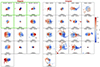 |
Fig. A.1. As in Fig. 9, but for the moment-1 HR maps. The thicker contour shows the systemic velocity. Subsequent contours are spaced by 25 km s−1. |
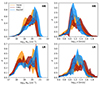 |
Fig. A.3. As in Fig. 6, but using the H2-to-H I partition recipe of Gnedin & Kravtsov (2011). Compared to the Blitz & Rosolowsky (2006) prescription, the column density range spanned by the FIRE-2 galaxies is compressed to lower values and the tail at NHI > 1021 cm−2 has disappeared. |
All Tables
Main properties of the five galaxies observed with MeerKAT and analysed in this study.
Characteristic parameters for the H I datacubes of the observed and simulated galaxy samples.
All Figures
|
Fig. 1. MeerKAT galaxy sample studied in this work. The high-resolution (∼22″) and low-resolution (∼65″) cases (HR and LR) are shown separately in the top and bottom parts of the figure. Top panels: H I column density iso-contours overlaid on top of grz colour-composite images from the DESI Legacy Imaging Surveys (Dey et al. 2019). Contours are drawn from primary-beam corrected moment-0 maps at NHI levels of 1019, 1020 (thicker line), 1020.5, and 1021 cm−2. The LR panels show an additional contour at the level of 1018 cm−2, in cyan. Bottom panels: Moment-2 maps. The velocity colour scheme is shown in the rightmost panels. |
| In the text | |
|
Fig. 2. Molecular-to-atomic hydrogen mass ratio as a function of galaxy stellar mass for the TNG50 (circles) and FIRE-2 (stars) systems studied in this work. All masses are computed within 100 kpc from the galaxy centre. Different H2/H I partition recipes are shown with different colours: green for Gnedin & Kravtsov (2011, GK11), red for Krumholz (2013, K13), and blue for Blitz & Rosolowsky (2006, BR06). The recipe of BR06 is the one that best reproduces the observational values from the xGASS Survey (Catinella et al. 2018), which are represented here by the shaded region. |
| In the text | |
|
Fig. 3. Main scaling properties of the simulated galaxy samples compared to various observational datasets. Left panel: SFR vs M⋆ for MHONGOOSE (dB24, blue squares), J0342-47 (light blue hexagon), HALOGAS (Heald et al. 2011; Kamphuis et al. 2022, cyan diamonds), and our TNG50 (orange circles) and FIRE-2 (dark red stars) samples. The blue dashed line shows the SDSS main sequence from Chang et al. (2015). The grey circles show the other systems from the MW/M31 TNG50 sample of Pillepich et al. (2024). Right panel: MHI vs M⋆. The markers are as in the left panel, with the addition of the SPARC sample (Lelli et al. 2016, green triangles). The purple-shaded area shows the ±1σ confidence region around the median scaling found by Maddox et al. (2015), while the blue dashed line shows the linear fit to the H I-WISE data from Parkash et al. (2018). Masses for the simulated galaxies are computed within 100 kpc from their centre. Black-edged markers are used for systems that are studied in this work. For comparison, we also show the simulated galaxies with H I masses computed with the recipe of Gnedin & Kravtsov (2011) (empty stars and circles). |
| In the text | |
|
Fig. 4. Diagnostic maps of galaxy 543376 in the TNG50 simulation. Top row: H I column density map down to a depth of 1016 cm−2 (left), stellar surface density map overlaid with H I contours (middle), H I metallicity map overlaid with the vector velocity field (right). Central and bottom rows: Moment maps for the HR (central) and LR (bottom) mock H I data, derived with SoFiA. The main galaxy properties are listed in the leftmost panel of the central row. The iso-contours in the NHI maps are drawn at levels of 1016, 1017 (in grey, top panel alone), 1018 (in blue, top and bottom panels), 1019, 1020, 1020.5, and 1021 cm−2 (in black, all panels), with the iso-contour at 1020 cm−2 highlighted with a thicker line. In the moment-1 maps, the contour at the systemic velocity is shown by a black line, and consecutive contours are spaced by 25 km s−1. The beam sizes are shown as red ellipses in the bottom right corner of the moment-0 maps. The dashed grey iso-contours in the top left panel trace the surface density distribution of the dark matter halo. |
| In the text | |
|
Fig. 5. Two-dimensional density histograms of the inclination-corrected H I column density and second moment values for MeerKAT (left panels), TNG50 (central panels), and FIRE-2 (right panels) galaxies. The top and bottom panels show the HR and LR cases, respectively. The black contours encompass 25%, 50%, 75%, and 95% of the highest density gas of the integrated distribution. The red dashed contours in the TNG50 and FIRE-2 panels reproduce the outermost contour of the MeerKAT distribution, and are included as a reference. |
| In the text | |
|
Fig. 6. Probability density distribution of inclination-corrected NHI values (left panels) and second moment values (right panels) for MeerKAT (blue), TNG50 (orange), and FIRE-2 (dark red curves) galaxies. The HR and LR cases are shown in the top and bottom panels, respectively. The solid lines show the median distribution for a given galaxy sample, while the shaded regions show the scatter within the sample, computed as the difference between the 84th and 16th percentiles. |
| In the text | |
|
Fig. 7. Cumulative H I flux as a function of the projected distance from the galaxy centre for individual MeerKAT (blue), TNG50 (orange), and FIRE-2 (dark red) systems (HR case). Abrupt discontinuities due to the presence of isolated H I-rich satellites have been removed from all profiles. |
| In the text | |
|
Fig. 8. Distribution of the fraction of spaxels with H I column densities below 1020 cm−2 for the LR cubes in MeerKAT (filled blue histogram), TNG50 (hatched orange histogram), and FIRE-2 (hatched dark red histogram). The fraction is computed with respect to all spaxels that contribute to the moment maps. |
| In the text | |
|
Fig. 9. Moment-0 maps for all galaxies in our sample divided into regular (on the left) and irregular (on the right), depending on whether the fraction f of spaxels with H I column density below 1020 cm−2 is higher or lower than 0.65 (see Fig. 8). f values of individual galaxies are annotated in each panel. The red dots mark TNG50 galaxies that have AGN feedback in thermal mode. The black iso-contours from the HR maps are drawn at levels of 1019, 1020 (thicker line), 1020.5, and 1021 cm−2. An additional iso-contour from the LR maps at 1018 cm−2 is shown in blue. The green boxes highlight galaxies observed with MeerKAT. The maps were derived with SoFia-2, using the same parameters for all galaxies. |
| In the text | |
|
Fig. 10. As in Fig. 6 for the HR case, but with the simulated galaxies split into regulars (top panels) and irregulars (bottom panels). Regular TNG50 galaxies follow the distributions observed with MeerKAT very well. |
| In the text | |
|
Fig. 11. Radial velocities (top panels) and gas mass flow rates (bottom panels) computed in spherical concentric shells, as a function of the shell radius, for the TNG50 (orange) and FIRE-2 (dark red) galaxies. Panels (a) and (d) show the inflow and outflow components separately, panels (b) and (e) show the net (outflow-inflow) flow for all gas phases, panels (c) and (f) show the net flow for the H I alone. The thick lines show the median trend, while the shaded areas show the difference between the 84th and 16th percentile. Negative values indicate inflow. |
| In the text | |
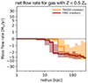 |
Fig. 12. As in panel (e) of Fig. 11, but for all gas with Z < 0.5 Z⊙. |
| In the text | |
|
Fig. 13. Distribution of the local environment estimator Nenv, defined as the number of companions with M⋆ > 107.5 M⊙ and MHI > 107 M⊙ detected within 250 kpc of projected distance and ±500 km s−1 of line-of-sight velocity from the main galaxy, for the MeerKAT (blue histogram) and the TNG50 (orange histogram) galaxy samples. The densely and sparsely hatched histograms show the regular and irregular TNG50 populations, respectively (see Fig. 9). |
| In the text | |
|
Fig. 14. Mass accretion rate of metal-poor gas (Z < 0.5 Z⊙), computed around r = r200 ≃ 200 kpc, as a function of the environment estimator Nenv, for TNG50 galaxies. The error bars account for the combined effect of galaxy-to-galaxy scatter and radial fluctuations in the Ṁ estimate around r200 in individual systems. The diamond and square markers show, respectively, the regular and irregular galaxies with Nenv = 0. Galaxies with more satellites show larger accretion rates. |
| In the text | |
|
Fig. 15. SFR surface density distribution in TNG50 (orange filled histograms) and FIRE-2 (dark red histograms) galaxies, for the HR case. Each panel accounts for spaxels in a given range of H I velocity dispersion, indicated at the top. |
| In the text | |
|
Fig. 16. H I position-velocity diagrams on slices parallel to the kinematic major and minor axes (first and second rows of each panel set) for J0419-54 (top panels), the TNG50 system 543376 (central panels), and the FIRE-2 system m12f (bottom panels) for the HR case. All panels show the same velocity range on the y-axis. The slice thickness is four pixels (20″). Slice offsets are indicated on the top right corner of each panel. Contours are spaced by powers of two, the outermost being at an intensity level of 0.3 mJy beam−1 (2σnoise). A negative contour (−2σnoise) is shown in grey. The circles highlight the anomalous kinematic features. The rightmost panels show the total H I maps with the cuts parallel to the major and minor axes (solid and dashed lines, respectively) used in the pv-slices. |
| In the text | |
|
Fig. 17. Representative H I spectra for the FIRE-2 galaxy m12f (HR), extracted at the pixel positions indicated in the top left corner of each panel. The grey lines show the mock H I spectra, the red lines show the best-fit multi-Gaussian models, the blue lines show the individual Gaussian components. The number of components used is indicated in the top right corner of each panel. |
| In the text | |
|
Fig. 18. Results of our multi-Gaussian fitting for the TNG50 (orange), FIRE-2 (dark red), and MeerKAT (blue) galaxies. Top panels: Fraction of spectra modelled with N components (1 ≤ N ≤ 5). Bottom panels: Median value of the distribution of the Gaussian standard deviations computed for all line profiles modelled with N components, as a function of N. The different panels show our results for spaxels in different ranges of (inclination-corrected) H I column density, indicated at the top of each panel. The dashed and dotted curves in the leftmost panels show, respectively, the regular and irregular populations of simulated galaxies. |
| In the text | |
|
Fig. A.1. As in Fig. 9, but for the moment-1 HR maps. The thicker contour shows the systemic velocity. Subsequent contours are spaced by 25 km s−1. |
| In the text | |
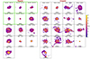 |
Fig. A.2. As in Fig. 9, but for the moment-2 HR maps. |
| In the text | |
|
Fig. A.3. As in Fig. 6, but using the H2-to-H I partition recipe of Gnedin & Kravtsov (2011). Compared to the Blitz & Rosolowsky (2006) prescription, the column density range spanned by the FIRE-2 galaxies is compressed to lower values and the tail at NHI > 1021 cm−2 has disappeared. |
| In the text | |
Current usage metrics show cumulative count of Article Views (full-text article views including HTML views, PDF and ePub downloads, according to the available data) and Abstracts Views on Vision4Press platform.
Data correspond to usage on the plateform after 2015. The current usage metrics is available 48-96 hours after online publication and is updated daily on week days.
Initial download of the metrics may take a while.