| Issue |
A&A
Volume 691, November 2024
|
|
|---|---|---|
| Article Number | A163 | |
| Number of page(s) | 24 | |
| Section | Extragalactic astronomy | |
| DOI | https://doi.org/10.1051/0004-6361/202449944 | |
| Published online | 11 November 2024 | |
PHANGS-MeerKAT and MHONGOOSE HI observations of nearby spiral galaxies: Physical drivers of the molecular gas fraction, Rmol
1
Argelander-Institut für Astronomie, Universität Bonn, Auf dem Hügel 71, 53121 Bonn, Germany
2
National Radio Astronomy Observatory, 520 Edgemont Road, Charlottesville, VA 22903, USA
3
Department of Astrophysical Sciences, Princeton University, 4 Ivy Lane, Princeton, NJ 08544, USA
4
Department of Astronomy, The Ohio State University, 140 West 18th Ave, Columbus, OH 43210, USA
5
Center for Cosmology and Astroparticle Physics, 191 West Woodruff Avenue, Columbus, OH 43210, USA
6
Max-Planck-Institut für Astronomie, Königstuhl 17, D-69117 Heidelberg, Germany
7
Department of Physics, University of Alberta, Edmonton AB T6G 2E1, Canada
8
Department of Astronomy, University of Cape Town, Private Bag X3, 7701 Rondebosch, South Africa
9
Kapteyn Astronomical Institute, University of Groningen, PO Box 800 9700 AV Groningen, The Netherlands
10
Netherlands Institute for Radio Astronomy (ASTRON), Oude Hoogeveensedijk 4, 7991 PD Dwingeloo, The Netherlands
11
European Southern Observatory, Karl-Schwarzschild Straße 2, D-85748 Garching bei München, Germany
12
Center for Astrophysics | Harvard & Smithsonian, 60 Garden Street, Cambridge, MA 02138, USA
13
Institute of Astronomy and Astrophysics, Academia Sinica, Astronomy-Mathematics Building, No. 1, Sec. 4, Roosevelt Road, Taipei 10617, Taiwan
14
National Radio Astronomy Observatory, 1003 Lopezville Road, Socorro, NM 87801, USA
15
Max-Planck-Institut für extraterrestrische Physik, Giessenbachstraße 1, D-85748 Garching, Germany
16
Universität Heidelberg, Zentrum für Astronomie, Institut für Theoretische Astrophysik, Albert-Ueberle-Straße 2, 69120 Heidelberg, Germany
17
Department of Physics & Astronomy, University of Wyoming, Laramie, WY 82071, USA
18
Department of Physics, University of Connecticut, Storrs, CT 06269, USA
19
Department of Physics and Astronomy, McMaster University, 1280 Main St. W., Hamilton, ON. L8S 4L8, Canada
20
Observatorio Astronómico Nacional (IGN), C/ Alfonso XII, 3, E-28014 Madrid, Spain
21
Astronomisches Rechen-Institut, Zentrum für Astronomie der Universität Heidelberg, Mönchhofstraße 12-14, D-69120 Heidelberg, Germany
22
Department of Physics, Tamkang University, No.151, Yingzhuan Road, Tamsui District, New Taipei City 251301, Taiwan
23
Center for Astrophysics and Space Sciences, Department of Physics, University of California San Diego, 9500 Gilman Drive, La Jolla, CA 92093, USA
24
Sub-department of Astrophysics, Department of Physics, University of Oxford, Keble Road, Oxford OX1 3RH, UK
⋆ Corresponding author; This email address is being protected from spambots. You need JavaScript enabled to view it.
Received:
11
March
2024
Accepted:
1
July
2024
Abstract
The molecular-to-atomic gas ratio is crucial to our understanding of the evolution of the interstellar medium (ISM) in galaxies. We investigated the balance between the atomic (ΣHI) and molecular gas (ΣH2) surface densities in eight nearby star-forming galaxies using new high-quality observations from MeerKAT and ALMA (for H I and CO, respectively). We defined the molecular gas ratio as Rmol = ΣH2/ΣHI and measured how Rmol depends on local conditions in the galaxy disks using multiwavelength observations. We find that, depending on the galaxy, H I is detected at > 3σ out to 20 − 120 kpc in galactocentric radius (rgal). The typical radius at which ΣHI reaches 1 M⊙ pc−2 is rH I ≈ 22 kpc, which corresponds to 1 − 3 times the optical radius (r25). We note that, Rmol correlates best with the dynamical equilibrium pressure, PDE, among potential drivers studied, with a median correlation coefficient of ⟨ρ⟩ = 0.89. Correlations between Rmol and the star formation rate surface density, total gas surface density, stellar surface density, metallicity, and ΣSFR/PDE (a proxy for the combined effect of the UV radiation field and number density) are present but somewhat weaker. Our results also show a direct correlation between PDE and ΣSFR, supporting self-regulation models. Quantitatively, we measured similar scalings as previous works, and attribute the modest differences that we do find to the effect of varying resolution and sensitivity. At rgal ≳ 0.4r25, atomic gas dominates over molecular gas among our studied galaxies, and at the balance of these two gas phases (Rmol = 1), we find that the baryon mass is dominated by stars, with Σ* > 5 Σgas. Our study constitutes an important step in the statistical investigation of how local galaxy properties (stellar mass, star formation rate, or morphology) impact the conversion from atomic to molecular gas in nearby galaxies.
Key words: galaxies: fundamental parameters / galaxies: ISM / galaxies: spiral
Jansky Fellow of the National Radio Astronomy Observatory.
NASA Hubble Fellow.
© The Authors 2024
 Open Access article, published by EDP Sciences, under the terms of the Creative Commons Attribution License (https://creativecommons.org/licenses/by/4.0), which permits unrestricted use, distribution, and reproduction in any medium, provided the original work is properly cited.
This article is published in open access under the Subscribe to Open model. This email address is being protected from spambots. You need JavaScript enabled to view it. to support open access publication.
1. Introduction
The accretion of cold gas from the circumgalactic medium is an important driver in the formation and evolution of galaxies. This cold gas first forms atomic hydrogen (H I) and then molecular hydrogen (H2), some of which eventually collapses under gravitational instability and forms new stars (Mac Low & Klessen 2004; McKee & Ostriker 2007; Klessen et al. 2016; Girichidis et al. 2020; Chevance et al. 2023). Stellar feedback also plays an important role in regulating the cold gas phase balance in galaxies via the photodissociation of H2 into H I due to radiation emitted by young stars. Consequently, H I is not only an intermediate gas phase in the star formation process but also one of its products (e.g., Allen et al. 1997; Heiner et al. 2011). The phase balance between atomic and molecular gas, often parameterized as the atomic-to-molecular gas ratio Rmol = ΣH2/ΣHI, encodes important information as to the evolution of the interstellar medium (ISM) in galaxies, from local environments in the Milky Way to distant, cold gas reservoirs in high redshift systems.
Atomic gas reservoirs are massive, extended, and often surround spiral galaxies far beyond their optical disks out to 2–5× the optical radius, r25 (e.g., Tamburro et al. 2009; Wang et al. 2016; Eibensteiner et al. 2023). The majority of the gas mass in galaxy disks is in H I but star formation occurs in H2 gas (see e.g. Schruba et al. 2011). The current abundance of molecular gas in galaxies reflects a balance between molecular cloud formation and destruction, with both large-scale dynamical processes and small-scale ISM physics playing important roles (e.g. see Dobbs et al. 2014; Sternberg et al. 2014; Saintonge & Catinella 2022; Chevance et al. 2023). On large scales, both theory and observations show that the mean pressure or density of the ISM affects the molecular-to-atomic gas ratio (e.g., Elmegreen 1989; Wong & Blitz 2002; Blitz & Rosolowsky 2004, 2006; Leroy et al. 2008; Ostriker et al. 2010; Mac Low & Glover 2012; Sun et al. 2020a) as do large-scale dynamical features such as spiral arm-induced shocks (Dobbs et al. 2014). Locally, metallicity and gas column density set the amount of shielding H I provides, which if sufficient can allow molecular gas to become dominant (Krumholz & Burkert 2010; Wolfire et al. 2010; Glover & Clark 2012; Sternberg et al. 2014, 2024; Smith et al. 2014; Schruba et al. 2018).
Elmegreen (1993) suggested that the ISM midplane pressure from dynamical equilibrium models determines the balance of the molecular and atomic phases of the ISM. They find that this pressure term is tightly related to the fraction of molecular gas and thus influences the fraction of ISM in the dense star-forming phase. Follow-up studies examined this and also found a tight relationship between the pressure term and Rmol (e.g., Wong & Blitz 2002; Blitz & Rosolowsky 2006; Leroy et al. 2008; Sun et al. 2020a) or the dense gas fraction traced by the HCN/CO line ratio1 (e.g., Usero et al. 2015; Jiménez-Donaire et al. 2019). Similar to these works, we refer to this term as the “dynamical equilibrium pressure” (PDE) throughout this paper. The availability of high-quality H I data is the main limiting factor in the abovementioned analyses, in terms of angular and spectral resolution, sensitivity, and methodology (i.e. fixing H I-related parameters). Because of the forthcoming and improved observations that capture the emission of low surface density H I together with the availability of multiwavelength data, the question arises whether Rmol is correlated with any other physical quantities (e.g. star formation rate, surface density, metallicity, radiation field). Assessing these relationships requires compiling both more sensitive H I observations and a suite of multiwavelength data.
Recently, many of the key required data have been assembled for a large set of galaxies in the context of the Physics at High Angular resolution in Nearby GalaxieS (PHANGS2) surveys (see, Leroy et al. 2021a,b; Emsellem et al. 2022; Sun et al. 2022) to revisit this analysis. One of the missing pieces has been high sensitivity H I observations. In this work, we fill this gap with new high-quality H I observations of eight nearby galaxies that are also in the PHANGS-ALMA sample, thus supported by available, comprehensive multiwavelength data. We analyze new H I observations taken with MeerKAT (the SKA precursor facility, Jonas & MeerKAT Team 2016) towards eight nearby galaxies and present the first comparison of new MeerKAT and ALMA observations to measure Rmol. As of 2024, MeerKAT is the most sensitive centimeter-wavelength interferometer in the southern hemisphere. The total MeerKAT antenna gain is ∼2.8 K/Jy and the system temperature is ∼18 K for the L band (856–1712 MHz) which makes it ideally suited to detect low column density H I emission (see e.g. de Blok et al. 2016, 2024; Elson et al. 2023; Boselli et al. 2023; Healy et al. 2024; Serra et al. 2019, 2023; Maccagni & de Blok 2024; Laudage et al. 2024).
In this paper, we measured how the molecular gas fraction (Rmol) depends on local conditions in galaxy disks. We conducted new measurements of Rmol for eight MeerKAT+ALMA data sets (see Sections 2, 3 and 4) and compared these to the total gas surface density (Σgas), the star formation rate surface density (ΣSFR), the stellar mass surface density (Σ*), the dynamical equilibrium pressure (PDE), and metallicity (Z(rgal)) (see Sections 5 and 6). This pilot study illustrates the power of MeerKAT and ALMA synergies to study key questions of galaxy evolution and reflects the best set of Rmol measurements based on the high sensitivity of these datasets.
2. MeerKAT 21-cm maps to compare with PHANGS-ALMA CO data
In this work, we analyze new H I observations taken with MeerKAT (the Square Kilometre Array (SKA) precursor facility, Jonas & MeerKAT Team 2016) towards eight nearby galaxies that are also in the PHANGS-ALMA sample and therefore have multiwavelength data available. Three of the eight galaxies are from ongoing efforts of the PHANGS collaboration to cover the PHANGS-ALMA sample with MeerKAT (Cycle 0 observations PI: D. Utomo, described in this work). Further, we include five more galaxies from the MeerKAT HI Observations of Nearby Galactic Objects – Observing Southern Emitters (MHONGOOSE, PI: W.J.G. de Blok) sample (de Blok et al. 2016).
2.1. New PHANGS-MeerKAT 21-cm observations of NGC 1512, NGC 4535, and NGC 7496
The observations were carried out using the South African MeerKAT radio telescope. The data for NGC 1512, NGC 4535, and NGC 7496 were taken between 2021 April 11 and 2021 June 14 for two times 3.5 h for each galaxy. The observations were taken using the 32k wide mode of the MeerKAT correlator, which provides 26.6 kHz wide channels (corresponding to 5.5 km s−1 at z = 0) and has a total bandwidth of 856 MHz. It is thus well suited to resolve the H I line and cover the full range of 21-cm emission from each galaxy. Each of the tracks consists of 10 min of observing time on the primary calibrator J1939−6342 followed by five cycles of two min on a phase calibrator and 3 hours on target.
2.1.1. Reduction
The observations of NGC 1512, NGC 4535, and NGC 7496 were reduced using the CASA-based IDIA calibration pipeline3 (see Collier et al. 2021). Briefly, the data were put through an initial flagging stage to eliminate regions of known persistent radio frequency interferences (RFI), flag known bad antennas, and identify the strongest RFI outside the known regions. This was followed by an initial round of continuum calibration using the 4K channel data4. We split out the parallel hand correlations (XX & YY) and used the primary calibrator to perform the bandpass calibration and flux scale bootstrapping. The secondary calibrator was used for phase calibration. We passed in the broadband model of the primary calibrator to get accurate fluxes across the band. This initial round of continuum calibration was followed by a second round of automated flagging of fainter RFI visible after a single round of calibration. The data were then processed through one final round of continuum calibration. We note that with the IDIA pipeline we do not perform frequency-dependent self-calibration. The continuum calibrated target was put through 2 rounds of phase-only self-calibration, using a pyBDSF mask to constrain the deconvolution to avoid artifacts. The first round is a 1 min phase-only solve, and the second round is a 10 min amplitude and phase solve. The continuum solutions were then transferred on the 32K channel data, that was subsequently used for imaging.
2.1.2. Imaging
We ran the calibrated data for the galaxies NGC 1512, NGC 4535, and NGC 7496 through a standard PHANGS product creation suite (similar to Leroy et al. 2021a; PHANGS-ALMA pipeline v3.05 using CASA 5.7.0-134), building noise cubes, strict masks at each resolution, and combined native+15″+30″+60″ broad masks. The PHANGS pipeline essentially uses the multiscale clean (with scales of 0, 30, 100, and 300″) followed by a more closely restricted single scale clean. We set robust = 0.5 and pblimit = 0.125 during imaging.
Prior to that, we used an order 1 baseline to subtract the continuum in the u − v-data, excluding the region around the spectral line in the galaxy itself. 1st order approximations are not always ideal and produced in our case some spectral curvature for some of the bright sources that could not be fitted with an order 1 u − v continuum subtraction. Rather than do anything more aggressive, we blanked the images in regions where a significant continuum was detected in the line-free channels after cleaning. More specifically, we picked the line-free channels manually and flagged all regions where S/N > 5 in the integrated map, allowing either positive or negative artifacts (i.e., we flagged absorption-like features too), then we also masked a couple of clearly problematic regions manually. These regions did not overlap the galaxy in any case. The biggest visible imaging artifacts remaining come from a bright continuum source to the southeast of NGC 7496 which shows some low-level artifacts. However, this is not enough to affect the overall noise.
After cleaning following the above procedure, we circularized the beam, which gives a slightly coarser resolution but also improves the signal-to-noise ratio (S/N). Our final working angular resolution for the images is 12″ − 15.0″. The rms noise is ∼0.20 − 0.22 mJy/beam (or ∼0.7 − 0.8 K) in the central part of the primary beam for all targets at this resolution (see Table 2). Although it is in principle possible to make higher resolution images with adjusted weighting in the future, a resolution of ∼15″ that corresponds to ∼1.5 kpc in the most distant galaxy is sufficient for our analysis.
2.2. HI data from MHONGOOSE
The galaxies IC1954, NGC 1566, NGC 1672, NGC 3511, and NGC 5068 are part of the MHONGOOSE survey (de Blok et al. 2016). The galaxies NGC 1566 and NGC 5068 were observed for ten 5.5 h tracks for a total of 55 h, and the remaining galaxies were already observed for 5.5 h as part of the MHONGOOSE survey (de Blok et al. 2024). Each of the tracks consists of 10 min of observing time on one of the primary calibrators J1939-6342 or J0408-6545. This is then followed by five cycles of two min on a phase calibrator and ∼55 min on the target galaxy. The c856M4k_n107M correlator mode was used, allowing for the 32k-narrow-band and 4k-wide-band to be used simultaneously. The narrow-band mode has 32 768 channels of 3.265 kHz width each, giving a total bandwidth of 107 MHz. The data were binned by two channels leading to a measurement set with a channel width of 6.53 kHz (1.4 km s−1).
2.2.1. Reduction
The data were processed using the publicly available CARACal data reduction pipeline6. The pipeline flags calibrators for RFI, derives and applies the cross-calibration, and flags the target. This is followed by self-calibration using the continuum. After applying the self-calibration solutions, the sky model derived in these steps is subtracted from the measurement set. A second round of uv-plane continuum subtraction using the line-free channels is then used to remove any residual continuum.
2.2.2. Imaging
Data cubes at various resolutions and weightings were created using wsclean (Offringa et al. 2014). Lower-resolution cubes were used to produce clean masks for the higher resolution cubes using the SoFiA-2 source finder (Westmeier et al. 2021). The data presented here use a robustness parameter of 0.5 and 1.5, resulting in an average beam size of 11″ and 30″, respectively. For our analysis, we use the higher resolution product (see Table 2). Moment maps were created with SoFiA-2 using the smooth+clip algorithm. We adopted spatial kernels at 0 and 1 times the beam size (i.e., 0 means no smoothing was applied) and spectral kernels of 0, 9, and 25 channels. In all cases, a source finding threshold of 4 sigma was used. A reliability value of 0.8 was used, but we found that in most cases this had little impact as the signal was well separated from the noise.
2.3. PHANGS-ALMA CO data and coverage
In addition to the MeerKAT 21-cm maps (from PHANGS-MeerKAT and the MHONGOOSE survey) introduced above, we use PHANGS-ALMA CO observations to investigate the molecular gas fraction. The PHANGS-ALMA survey maps the CO J = 2 − 1 line emission at ∼1″ angular resolution covering the area of active star formation in nearby disk galaxies (Leroy et al. 2021b). Although most of the CO emission is expected to lie within the targeted region, weak CO emission can extend into the outer disks of galaxies (e.g., Braine et al. 2007; Schruba et al. 2011; Koda et al. 2022). As mentioned in Section 4.6.1 of Leroy et al. (2021b) the PHANGS CO maps usually cover ∼70 − 90% of the total CO emission. This result is obtained by using the WISE3 (12 μm) observations, which show a surprisingly strong correlation with CO intensity, to make an effective aperture correction (see Section 4.6.1 in Leroy et al. 2021b for more details).
In this work, we use the emission from the low-J rotational transition of carbon monoxide (CO) as an observational tracer of the molecular gas. The use of CO emission as a H2 tracer comes, however, with a caveat. The H2 abundance is also influenced by the cosmic ray (CR) rate. While the CR rate diminishes at high column densities CRs are less affected by attenuation compared to UV radiation. Moreover, the conditions necessary for the formation of H2 and CO are not the same (see e.g. Gong et al. 2018): in equilibrium, the CO abundance depends primarily on the column density (CO requires AV > 1), whereas H2 forms more easily at lower AV because it is self-shielded. The upper limit on the H2 abundance (in self-shielded gas) depends on density through the balance between formation and CR destruction. It is, however, relevant for this work that CO, and not H2, determines the cooling rate in the ISM.
3. The sample
In this work we use a compiled dataset that contains new observations from the MeerKAT telescope targeting the galaxies NGC 1512, NGC 4535, and NGC 7496 from the first results of the PHANGS-MeerKAT survey along with the galaxies IC1954, NGC 1566, NGC 1672, NGC 3511, and NGC 5068 from the MHONGOOSE survey (de Blok et al. 2016) Taken together, this forms a sample of eight nearby (D = 5.2 − 19.4 Mpc) spiral galaxies (see Table 1). These eight galaxies are also part of the PHANGS-ALMA survey (Leroy et al. 2021b) and have archival multiwavelength observations available. In the following, we describe each galaxy shown in Figures 2 and 3 and give a brief literature overview.
Properties of our compiled dataset for NGC 1512, NGC 4535, and NGC 7496 (from PHANGS-MeerKAT; this work) and IC1954, NGC 1566, NGC 1672, NGC 3511, and NGC 5068 (from MHONGOOSE, de Blok et al. 2016).
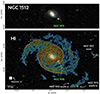 |
Fig. 1. Example of the extent of the emission of H I with the new MeerKAT observations. Top: three-color optical image showing star forming spiral galaxy NGC 1512 and the low-mass dwarf companion NGC 1510 in the optical (image credits: DESI Legacy Survey). The scale bar on the lower left corner indicates 20 kpc. Bottom: same as above but overlaid with H I emission contour levels of log10 0.25, 1, 1.5, 2, 2.25, 2.5, 2.75, 3 K km s−1 together with the western and southern tidal dwarf galaxies of NGC 1512 (see Section 3 for more information). |
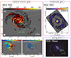 |
Fig. 2. Example of a multiwavelength view of one of our galaxies within our sample – NGC 1512. Left in red frame: MeerKAT H I observations showing on top the integrated intensity map in units of K km s−1 (moment 0), which we use in this work. Although not used in this paper, the bottom panels show the velocity field (moment 1) and the velocity dispersion (moment 2). These maps are used in Laudage et al. (2024) to analyze the neutral atomic and molecular gas kinematics in the PHANGS-MeerKAT sample. Right top in purple frame: ALMA observations of CO(2–1) from PHANGS-ALMA (Leroy et al. 2021b) showing an integrated intensity map (see Section 2.3 for CO coverage). Right bottom in blue frame: GALEX observation of FUV emission at 154 nm. The green rectangle shows the location of the interacting galaxy NGC 1510. |
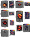 |
Fig. 3. Integrated intensity maps (moment 0) for H I emission (in red to yellow colors) and CO(2–1) (in purple to yellow colors) across the disks of our sample of eight nearby spiral galaxies (excluding NGC 1512, already shown in Figure 2). The corresponding beam sizes are visible in the bottom left corner of each map. The white dashed contours on the MeerKAT H I maps represent the field of view of the ALMA CO(2–1) observations, which we show next to each HI map. The CO maps cover ∼70 − 90% of the total CO emission (see Section 2.3). |
IC 1954. From the MeerKAT integrated intensity map we see bright H I emission (> 250 K km s−1) that extends ∼5 kpc in radius and is surrounded by fainter emission (∼50 K km s−1). The CO map reveals some spiral arm-like structures. The H I phase of this galaxy has not been studied in detail so far.
NGC 1512. We highlight the barred, double-ring galaxy NGC 1512 in Figure 2. Its inner H I distribution reflects the ring like structuring of the gas, which can also be seen in the CO map. More astonishing, however, are the two gigantic (more than 160 kpc in length7) spiral arms and the prominent disturbances of the H I emission in the southern part of the inner 20 kpc caused by the interacting low-mass dwarf companion NGC 1510, which is bright in H I emission. The southern arm splits at larger galactic radii into three sub-arms. The northern arm, on the other hand, is clumpier in structure and seems to follow only one direction at larger galactic radii (i.e., no splitting into sub-arms). The distribution and kinematics of the H I gas of this system have also been studied by Koribalski & López-Sánchez (2009) using the Australia Telescope Compact Array (ATCA). However, our map shows much more detail due to the higher resolution of the MeerKAT observations (15″ compared to a synthesized beam size of ≈88″ from ATCA). In addition to the splitting of the southern arm, our map shows additional clumps of H I emission in the south and east. These were characterized as tidal dwarf galaxies (TDG) by Koribalski & López-Sánchez (2009), who named them simply NGC 1512-south and NGC 1512-west, with both showing clear signs of star formation. In our H I map, however, NGC 1512-south appears as two separate emission clumps. Following the nomenclature we name them NGC 1512-south-a and NGC 1512-south-b. Within the PHANGS collaboration a detailed kinematic study of this H I disk together with the ones from NGC 4535 and NGC 7496 (marked as P–M in Table 2) is underway (Laudage et al. 2024).
Properties of our imaged dataset.
NGC 1566. In H I two remarkably prominent spiral arm-like features are visible with corresponding “inter-arm” regions. Both of these arms are winding clockwise, somehow forming a natural extension to the arms seen in CO. NGC 1566, also known as the “Spanish Dancer”, is an active galaxy classified as Seyfert 1 (Alloin et al. 1985; Malkan et al. 1998). H I is detected in absorption against the AGN, with corresponding H I mass about 7 × 10⁶ M⊙ (see Maccagni & de Blok 2024). Hence, even though depleted with respect to the CO, there is H I in the central regions tracing the neutral atomic counterpart of what was detected by ALMA in Combes et al. (2014). Within the MHONGOOSE collaboration a detailed study of this H I disk is under way (Maccagni & de Blok 2024).
NGC 1672. From the H I map it is hard to identify clear arm-like features. The H I gas seems to be not uniformly distributed, as we find higher integrated intensities along the northern edge of the H I disk. Also, regions within the field of view of the CO observations show higher integrated H I intensities (> 300 K km s−1) at two regions that are the intersections between a bar and the beginning of two spiral arm-like features – the bar ends. NGC 1672 is known to have a strong bar that is 2.4′ in length, which corresponds to 13.5 kpc at its distance of 19.4 Mpc. These bar ends are only faintly detected in CO. High-resolution optical imaging data from the Hubble Space Telescope (HST) reveal that the bar lane splits into two arms each (i.e., four spiral arms in total) with many HII regions and vigorous star formation along them (e.g. Jenkins et al. 2011; Barnes et al. 2022).
NGC 3511. The H I map shows no clear signs of spiral arm-like features. In CO, two very diffuse, thick, and patchy spiral arms are apparent, however, a clear identification is complicated due to the galaxy’s high inclination. The neighboring galaxy NGC 3513 is about 10 arcminutes away from NGC 3511. A filamentary structure with low integrated intensity spanning the two galaxies speculatively seems to connect them. Both galaxies have similar distance estimates of 14.19 Mpc (taken from the MHONGOOSE sample table, de Blok et al. 2024).
NGC 4535. The H I map reveals compact emission forming a disk ∼20 kpc in radius. In the outskirts, two spiral arm-like structures are present, forming (similar to the ones in NGC 1566, but not as prominent) a natural extension to the arms seen in CO. The observed HI spiral arm-like structures in NGC 4535 resemble those typically influenced by ram pressure, leading to the ‘unwinding’ of spiral arms in cluster galaxies (see Bellhouse et al. 2021). Given that NGC 4535 is a member of the Virgo Cluster, it is plausible that similar processes are at play in this galaxy as well.
NGC 5068. The H I disk of NGC 5068 has a diameter of ∼10 kpc and shows no clear sign of spiral arm-like structures. NGC 5068 is classified as Sc, is the closest galaxy in our sample with a distance of ∼5.2 Mpc, and has the lowest total molecular gas mass, the lowest total mass of stars and the lowest star formation rate in our sample (see Table 1). Apart from the properties mentioned in this table, relatively little is known about this galaxy. Within the MHONGOOSE collaboration, a detailed study of this H I disk is was conducted by Healy et al. (2024).
NGC 7496. NGC 7496’s appearence in H I is somewhat different compared to the other galaxies. Its H I map reveals an inner compact disk that is surrounded by a symmetric ring-like structure that could be the extensions of the inner two spiral arms. These spiral arm like features are even more evident in the CO map.
4. Derivation of physical quantities
Our goal in this work is to measure the H2-to-H I ratio, Rmol, and to compare it to a set of local environmental factors that, theoretically, have a bearing on the balance of atomic and molecular gas. To identify large-scale conditions associated with total molecular abundance in the ISM, we use a variety of different physical quantities: the atomic gas surface density (ΣHI, Section 4.1), molecular gas surface density (ΣH2, Section 4.2), total gas surface density (Σgas, Section 4.3), star formation rate surface density (ΣSFR, Section 4.4), stellar mass surface density (Σ*, Section 4.5), dynamical equilibrium pressure (PDE, Section 4.6), the ratio between the star formation rate per unit area and dynamical equilibrium pressure (ΣSFR/PDE) as a proxy for the balance between molecular gas formation versus dissociation (see Section 4.7), and ISM metallicity (Z′, normalized to the solar value, Section 4.8).
We extract measurements in a set of 1.5 kpc hexagonal apertures8 that completely tile the sky footprint of each galaxy. This is the same sampling scheme used in Sun et al. (2022) and allows us to leverage a rich set of existing measurements made available by that work (see, for example, Figure 4). We note that this approach does not require us to convolve the data first to a common beamsize using a Gaussian kernel. We refer interested readers to Sun et al. (2022) for more information. Below we briefly describe how we derive various physical properties.
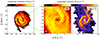 |
Fig. 4. Integrated intensity maps after hexagonal sampling. The left plot shows the overall H I disk of NGC 1566. The right two panels show the enlarged versions of the green rectangle at matched field-of-view. We show here hexagonal apertures (1.5 kpc in size) on the H I and CO(2–1) maps where the circle in the lower left corner indicates the (matched) beam size (see Table 2). |
4.1. Atomic gas surface density
Assuming optically thin H I emission, we convert IHI from the MeerKAT observations (see Section 2) to atomic gas surface density ΣHI via,
![Mathematical equation: $$ \begin{aligned} {\Sigma _{\rm HI}}\,[\,\mathrm{M_\odot \,pc}^{-2}] = 2.0\times 10^{-2}~I_{\rm HI}\,[\mathrm{K\,km\,s}^{-1}]~\cos {(i)}. \end{aligned} $$](/articles/aa/full_html/2024/11/aa49944-24/aa49944-24-eq1.gif) (1)
(1)
Here ΣHI includes the (extra 35%) mass of helium and heavier elements. The cos(i) term accounts for galaxy inclination taken from Table 1. A note of caution is appropriate, as the inclination angle has been seen to vary in the outskirts of galaxies induced by significant warps and tidal effects from infalling galaxies or gas streamers. The main results of this paper should not be impacted by the assumption of a constant inclination angle. In the future, these new maps will yield additional constraints on the inclination and the position angle (for example, Laudage et al. 2024 for NGC 1512, NGC 4535, and NGC 7496).
4.2. Molecular gas mass surface density
We estimate the molecular gas mass surface density, ΣH2, from the CO integrated intensity taken from the PHANGS-ALMA survey (Leroy et al. 2021b) via,
![Mathematical equation: $$ \begin{aligned} {\Sigma _{\rm H2}}\,[\mathrm{M_\odot \,pc}^{-2}] = \alpha _{\rm CO(1{-}0)}\,R_{21}^{-1}~I_{\rm CO}\,[\mathrm{K\,km\,s}^{-1}]~\cos {(i)}. \end{aligned} $$](/articles/aa/full_html/2024/11/aa49944-24/aa49944-24-eq2.gif) (2)
(2)
For the CO line ratio (R21) and CO(1–0)-to-H2 conversion factor (αCO(1 − 0)) we adopt R21 = 0.65 from den Brok et al. (2021) and Leroy et al. (2022) and use a metallicity-dependent αCO prescription as described in Accurso et al. (2017) and Sun et al. (2020b) as αCO(1 − 0) = 4.35 Z′ − 1.6 M⊙ (K km s−1 pc2)−1, where Z′ is the inferred local gas phase O/H abundance normalized to the solar value (see Section 4.8)9. Again, ΣH2 includes the (extra 35%) mass of helium and heavier elements. The same cos(i) inclination correction from Equation (2) also applies here.
4.3. Total gas surface density and molecular gas fraction
We estimate the total gas surface density, Σgas from the sum of Eqs. (1) and (2) as,
![Mathematical equation: $$ \begin{aligned} \Sigma _{\rm gas}\,[\mathrm{M_\odot \,pc}^{-2}] = {\Sigma _{\rm HI}+\Sigma _{\rm H_2}}. \end{aligned} $$](/articles/aa/full_html/2024/11/aa49944-24/aa49944-24-eq3.gif) (3)
(3)
We estimate the molecular gas fraction, Rmol = H2-to-H I, by taking the ratio as,
![Mathematical equation: $$ \begin{aligned} R_{\mathrm{mol}} = \frac{{\Sigma _{\rm H2}}\,[\mathrm{M_\odot \,pc}^{-2}]}{{\Sigma _{\rm HI}}\,[\mathrm{M_\odot \,pc}^{-2}]}. \end{aligned} $$](/articles/aa/full_html/2024/11/aa49944-24/aa49944-24-eq4.gif) (4)
(4)
For measuring the molecular gas fraction, we include non-detections. For the case of no significant detection (i.e., below a signal-to-noise ratio of 3) in ΣH2 we replace the values with upper limits (3 times the uncertainty) and include the propagated errors. We report for only one 1.5 kpc sized aperture in one galaxy (NGC 7496, see Section 5.1) a non-detection in ΣHI where we detect ΣH2, and thus, we do not include lower limits in our Rmol measurements.
4.4. Star formation rate surface density
We estimate the star formation rate (SFR) surface density ΣSFR by combining ultraviolet (UV) data from the Galaxy Evolution Explorer (GALEX; Martin et al. 2005) and mid-infrared (mid-IR) data from from the Wide-field Infrared Survey Explorer (WISE; Wright et al. 2010), following a new SFR calibration (Belfiore et al. 2023). In detail, we make use of the FUV 154 nm, near-IR 3.4 μm (WISE1), and mid-IR 22 μm (WISE4) data. These datasets were processed as part of the z0MGS project (Leroy et al. 2019).
Building upon Leroy et al. (2019), Belfiore et al. (2023) refined the FUV+WISE4 star formation rate prescription by introducing an additional dependence on the local FUV-to-WISE1 color. This refinement corrects for contamination by IR cirrus in WISE4 bands, leading to better agreement in the SFR estimates from FUV+WISE4 versus those from extinction-corrected Hα. The refined prescription can be expressed as
![Mathematical equation: $$ \begin{aligned} \Sigma _{\rm SFR}\,[\mathrm{M_\odot \,yr^{-1}\,kpc}^{-2}] = C_{\rm FUV} L_{\rm FUV} + C_{\rm W4}^\mathrm{FUV} L_{\rm W4}, \end{aligned} $$](/articles/aa/full_html/2024/11/aa49944-24/aa49944-24-eq5.gif) (5)
(5)
where CFUV is the FUV conversion factor established by Leroy et al. (2019), that is based on SED fitting results of Salim et al. (2018), using a Chabrier (2003) IMF.  is the conversion factor in units of M⊙ yr−1/(erg s−1). In our case, we take their recommendation of
  depending on Q ≡ LFUV/LW1, a broken power law in the form of,
 (6)
(6)
where Qmax = 0.60, a0 is log Cmax − a1 log Qmax, with a1 = 0.23, log Cmax = 0.60 (see also Table 3 and Equation (7) in Belfiore et al. 2023). This description is better at mitigating the IR cirrus contamination.
We show in Appendix A a comparison of our SFR measurements with Hα-based SFR measurements that are corrected for dust extinction based on the Balmer decrement (see Belfiore et al. 2023) for the 5 out of our 8 galaxies that are in the PHANGS-MUSE sample (Emsellem et al. 2022). We find that the Hα-based ΣSFR show a similar trend but with smaller scatter and thus might reveal a tighter relationship between Rmol and ΣSFR.
4.5. Stellar mass surface density
We use the stellar mass surface density Σ* maps computed with the technique utilized for the PHANGS-ALMA survey (Leroy et al. 2021b). This Σ* estimate is based on near-infrared emission observations at 3.6 μm (IRAC1 on Spitzer, from the S4G survey; Sheth et al. 2010) or 3.4 μm (WISE1, from the z0MGS project; Leroy et al. 2019). The final stellar mass is then derived from the NIR emission using a mass-to-light ratio, Υ3.4 μm, that depends on the local specific star formation rate SFR/M⋆,
![Mathematical equation: $$ \begin{aligned} {{\Sigma _{*}}}[\mathrm{M_\odot \,pc}^{-2}]&= 350 \left(\frac{\Upsilon _{\rm 3.4\,\upmu m}}{0.5}\right)~{I_{\rm 3.6\,\upmu m}}~[\mathrm{MJy\,sr}^{-1}]~ \cos {(i)}. \end{aligned} $$](/articles/aa/full_html/2024/11/aa49944-24/aa49944-24-eq9.gif) (7)
(7)
4.6. Dynamical equilibrium pressure
In general, the dynamical equilibrium pressure is the expected average ISM pressure near the galaxy mid-plane needed to balance the weight of the ISM (per unit area) in the galaxy’s gravitational potential. We derived the kiloparsec-scale dynamical equilibrium pressure, PDE, in the same way as in Sun et al. (2020a) that is based and built on considerable previous work (Spitzer 1942; Elmegreen 1989; Wong & Blitz 2002; Blitz & Rosolowsky 2004, 2006; Leroy et al. 2008; Ostriker et al. 2010; Kim et al. 2011, 2013). We calculate PDE under the assumptions that (i) the distribution of gas and stars in a galaxy disk can be treated as isothermal fluids in a plane-parallel geometry, (ii) the (single component) gas disk scale height is much smaller than the stellar disk scale height, (iii) gravity due to dark matter can be neglected since it represents only a minor component in the inner disk (the relevant region where we can calculate PDE) of massive galaxies. PDE can then be expressed as the sum of the weight of the ISM due to its self-gravity (see e.g. Spitzer 1942; Elmegreen 1989) and the weight of the ISM due to the stellar potential (see e.g. Spitzer 1942; Blitz & Rosolowsky 2004):
![Mathematical equation: $$ \begin{aligned} P_{\rm DE}\ [k_{\rm B} \mathrm{K\,cm^{-3}}] = \left(\frac{\pi \ G}{2}\Sigma ^2_{\rm gas}+\Sigma _{\rm gas}\sqrt{2G\rho _{*}}\sigma _{\mathrm{gas},z}\right). \end{aligned} $$](/articles/aa/full_html/2024/11/aa49944-24/aa49944-24-eq10.gif) (8)
(8)
Here, Σgas is the total gas surface density (see Section 4.3), and ρ* is the stellar mass volume density near the disk midplane that we can describe as
 (9)
(9)
This is under the assumption of an isothermal density profile along the vertical direction and a fixed stellar disk flattening ratio r*/h* = 7.3, where r* is the radial scale length of the stellar disk and h* its scale height. We take r* for each galaxy in our sample from Leroy et al. (2021b). These scale lengths have been derived from the S4G photometric decompositions of 3.6 μm images (IRAC1 on Spitzer; Sheth et al. 2010). Sun et al. (2020a) compared this way of calculating ρ* with a flared disk geometry and found that the latter scenario gives lower PDE values. In Eq. (8), σgas, z is the mass-weighted average velocity dispersion of the molecular and atomic gas phases in the direction perpendicular to the disk plane,
 (10)
(10)
To be able to compare our pressure estimates to previous works, we follow Sun et al. (2020a) and adopt a fixed σatom of 10 km s−1 (taken from Leroy et al. 2008), which holds on 1.5 kpc scales. However, we compare in Appendix C our calculated PDE estimates with the ones where we let σatom vary and find overall small differences between these two methods, in agreement with Sun et al. (2020a). According to these authors the assumption of a fixed σatom leads to generally higher PDE. For both ρ* and σatom the resulting deviation lies within 0.2 dex. These are minor differences and therefore should not have too much of an impact, which is why in this work we (i) take a fixed stellar disk flattening ratio, and (ii) fix σatom.
4.7. PDE/ΣSFR as a proxy for physical conditions driving molecular-to-atomic transition
Models of photodissociation and cosmic ray (CR) dissociation argue that H2 formation depends on both gas density and UV / CR radiation field (e.g., Hollenbach & Tielens 1999; Gong et al. 2018). Within a given cloud with density ncloud, we expect an increase in molecular abundance with ncloud/G0 or ncloud/ξCR – the density in cold clouds over the UV radiation field or cosmic ray rate. Along this line, Elmegreen (1993) considered cloud populations existing under given external ISM pressure and UV radiation field and concluded that the molecular abundance inside these clouds should depend positively on the external pressure and negatively on the radiation field.
In light of these theoretical considerations, here we use the ratio of PDE/ΣSFR to capture the combination of key physical parameters determining the molecular gas fraction. PDE represents an observational proxy of the external pressure considered by Elmegreen (1993); it is also known to correlate strongly with molecular cloud internal pressure (Sun et al. 2020a), which in turn follows scaling relations with cloud surface/volume densities (Sun et al. 2018, 2020b; Rosolowsky et al. 2021). ΣSFR is expected to scale linearly with G0 and ξCR as both UV photons and CR come from young stars and stellar remnants created in recent star formation events. Taken all these together, we expect PDE/ΣSFR to reflect the balance of molecular gas formation versus dissociation, which could drive variations in the molecular gas fraction, Rmol.
4.8. ISM Metallicity
Following Sun et al. (2022), we use in this work the scaling relations to obtain the general trends of ISM metallicity variation across our sample of eight galaxies. We assume a global galaxy mass–metallicity relation (Sánchez et al. 2019) and a fixed radial metallicity gradient within each galaxy (Sánchez et al. 2014), which gives,
 (11)
(11)
where Z′(rgal) is the normalized abundance at arbitrary rgal and Z′(re) is the local gas-phase abundance at rgal = re normalized by the solar value [12 + log(O/H) = 8.69],
 (12)
(12)
M⋆ in Eq. (12) is the galaxy’s global stellar mass under the assumption of a Chabrier IMF (Chabrier 2003). Note that these scaling relations are appropriate for abundance measurements adopting the O3N2 calibration in Pettini & Pagel (2004). For more details see the appendix in Sun et al. (2022). We show in Appendix B a comparison of metallicity measurements, where we include metallicities of individual H II regions for the galaxies that are in the PHANGS-MUSE sample (Groves et al. 2023).
4.9. Scaling relations and propagated errors
We characterize scaling relations by including measurement errors and upper limits, using the hierarchical Bayesian method described in Kelly (2007). This approach is available as a python package: linmix10. It performs a linear regression of y on x while incorporating measurement errors in both variables and accounting for non-detections (upper limits) in y. The regression assumes a linear relationship in the form of
 (13)
(13)
where β is the slope, and α is the y-intercept. We use this approach for Section 5.3.
We derive the propagated errors (σprop) of the ratios between quantities (Iratio) as:
 (14)
(14)
The errors are expressed on a base 10 logarithmic scale as:
 (15)
(15)
5. Results
In this section, we present the results from the MeerKAT and ALMA observations of our sample of eight nearby galaxies (from the PHANGS and MHONGOOSE surveys). Figures 2 and 3 show the H I and CO moment maps of our sample. We describe the radial extent of H I and CO emission (see Figures 5, 6, 7 and 8) in Sections 5.1 and 5.2. Using ancillary data (described in Section 4) we analyze Rmol scaling relations (see Figure 9) in Section 5.3.
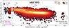 |
Fig. 5. Radial extent of H I and CO in NGC 1512. This galaxy has the largest H I disk in our sample. The maximum galactocentric radius of the CO(2–1) observations is sensitive to the ALMA field-of-view (we recover ∼70 − 90% of the total CO emission, see Section 2.3). The scatter points show each individual sight line, i.e. 1.5 kpc aperture. The red-to-yellow color scale shows the point density of ΣHI and the dark-blue to yellow shows the point density of ΣH2. The white and red lines show the median within a given 1.5 kpc wide radial bin. We see that H I extends until rgal ∼ 120 kpc (that is 5 × r25 or 8 times the optical radius of the Milky Way, indicated as a purple arrow). We indicate the approximate rgal range where NGC 1510 sits with vertical dashed lines. The clumps NGC 1512-south-a, NGC 1512-south-b, and NGC 1512-west are ∼140 kpc from the center of NGC 1512. We indicate Reff, r25 and RHI as gray, pink, and orange vertical dashed lines, respectively (taken from Table 1). |
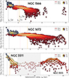 |
Fig. 6. Radial extent of H I and CO in NGC 1566, NGC 1672, and NGC 3511. These galaxies have the largest H I disk extent in our sample, and exhibit special H I characteristics. We indicate Reff, r25 and RHI as grey, pink, and orange vertical dashed lines, respectively (taken from Table 1). Top: we note here two additional clumps outside of NGC 1566’s main H I disk that have been identified as additional field galaxies (see de Blok et al. 2024). Middle: toward NGC 1672 we see an increase of H I emission at rgal ∼ 70 kpc, which is the region of additional low-H I emission in the west of NGC 1672’s disk (see also Figure 3). Bottom: The hatched region from rgal = 40-120 kpc spans the low-density filamentary structure seen in the moment map (see Figure 3), which gives the impression of connecting NGC 3511 and NGC 3513. |
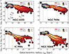 |
Fig. 7. Radial extent of H I and CO in NGC 4535, NGC 7496, IC 1954, and NGC 3511. These galaxies have the smallest H I disk extent in our sample, and do not exhibit any peculiar H I characteristics. We show the corresponding Reff, r25 and RHI indicated as vertical dashed lines. |
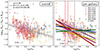 |
Fig. 8. Rmol against the normalized radius rgal/r25. The region below the dotted horizontal line at Rmol = 1 can be viewed as dominated by ΣHI, and the region above that line by ΣH2. Left: grey line shows a fit for all the galaxies and it crosses the Rmol = 1 boundary at rgal ∼ 0.4 r25, which means that the atomic gas on average becomes molecular inside that radius in these eight galaxies. The grey shaded region corresponds to the 3σ confidence interval. Right: colored lines show fits for individual galaxies. We list the corresponding fit parameters in Table 4. |
5.1. Radial extent of the surface density of the atomic and molecular gas
In Figures 5, 6 and 7 we show the radial extent of ΣHI and ΣH2 together with their point densities, with galaxies grouped by their H I disk extent and special H I characteristics. To derive radial trends we bin ΣHI and ΣH2 in galactocentric bins of 1.5 kpc width (the common beam size, i.e. the size of our hexagonal apertures). The white and red lines thus represent the median ΣH2 and ΣHI respectively, within a given bin.
Carefully inspecting each individual galaxy map reveals additional clumps, dips, or peaks at larger rgal, and/or companion galaxies. In Figure 5 showing NGC 1512, H I extends out to rgal ∼ 120 kpc (that is 8× the radius of the Milky Way, indicated as a purple arrow). NGC 1512’s interacting companion (NGC 1510) is indicated by a grey shaded region at rgal = 16 − 20 kpc. The clumps NGC 1512-south-a, NGC 1512-south-b, and NGC 1512-west are ∼140 kpc from the center of NGC 1512 and are most likely tidal dwarf galaxies. Additionally, we see an increase in both ΣHI and ΣH2 at rgal ∼ 8 kpc, which is the location of the ring-like feature that can be seen in Figure 2.
In Figure 6 we show the radial extent of NGC 1566, NGC 1672, and NGC 3511. In NGC 1566 H I extends until rgal ∼ 55 kpc with two additional clumps at rgal ∼ 65 kpc and rgal ∼ 97 kpc, that have been identified as additional field galaxies, LEDA 414611 and LSBG F157-052 (see de Blok et al. 2024). For NGC 1672 H I extends until rgal ∼ 65 kpc. The H I extent in NGC 3511 is dominated by other features besides the steep radial decline in ΣHI. The hatched region indicates the filamentary structure with low integrated intensity, followed by the companion galaxy NGC 3513.
In Figure 7 we show the galaxies in our sample that have the least extended H I disks and/or do not exhibit special characteristics such as clumps or connecting branches. NGC 4535 reaches rgal ∼ 40 kpc. IC 1954, NGC 5068 and NGC 7496 show a maximal H I extent of ∼25 kpc. We do not detect any H I emission in the inner 1.5 kpc for NGC 7496. This can also be seen in the moment 0 map in Figure 3. IC 1954, NGC 5068 and NGC 7496 are those with the lowest total stellar mass (M⋆) in our sample (see Table 1).
Inspecting environmental differences reveals that almost all of our galaxies show higher ΣH2 than ΣHI in their central 1.5 kpc (except NGC 7496 as aforementioned). We find that ΣHI in these central regions does not surpass ∼8 M⊙ pc−2 (similar to what has been found in Bigiel et al. 2008). NGC 1566 and NGC 1672 are the galaxies that stand out the most in our sample, each having ΣH2 ∼ 3 orders of magnitude higher than ΣHI in their central regions.
For our sample, we find a range of maximum radial extent of ΣHI of rgal, max ≈ 20 − 120 kpc, and for ΣH2 we find rgal, max ≈ 5 − 18 kpc. The measurements of rgal, max are based on the detection threshold of at least 3σ. The H I emission is on average 5 times more extended than the detected CO emission (see also Table 3). We remind the reader that the maximum galactocentric radius of the CO(2–1) observations is sensitive to the ALMA FoV. We expect, however, that we cover ∼70 − 90% of the total CO emission (see Section 2.3). It is common to use the ΣHI = 1 M⊙ pc−2 isophote definition for the maximal radial extend of ΣHI, which we indicate as rHI in Table 3 and find rHI ≈ 6 − 65 kpc. We find that on average rHI is approximately twice the radial position of the B-band isophote at 25 mag arcsec−2 (i.e., rHI ≈ 2r25) and six times the radius that contains half of the stellar mass of a galaxy (i.e., rHI ≈ 6reff). Notably, NGC 1512 has a much larger H I extent than this average trend, with rHI ≈ 3r25 or rHI ≈ 14reff.
Radial extent of our sample.
5.2. The transition from atomic to molecular gas dominated regimes
We aim to measure at what radius in our galaxies the overall molecular gas surface density is equal to that of the atomic gas. This represents the boundary between the regions where either H I or H2 dominates. To compare galaxies with different stellar radial extents, it is common to normalize the galactocentric radius (rgal) with r25. In Figure 8 we show Rmol versus rgal/r25. The rainbow-colored symbols show individual 1.5 kpc apertures within each galaxy. We note that all the galaxies within our sample contribute with a similar amount of individual aperture measurements (median number of sightlines = 115). In the left panel, the gray linear regression fit shows the correlation of Rmol and rgal/r25 in the form of log10(y) = β × (x)+α across all galaxies, which we find to be
 (16)
(16)
The fit crosses the Rmol = 1 boundary (in log scale indicated as a horizontal line at 0) at rgal ∼ 0.4 r25. However, looking at individual galaxies in the right panel of Figure 8, such as NGC 1512 or NGC 1566, reveals that for these objects ΣHI already dominates at a smaller rgal/r25, whereas in other galaxies Rmol crosses the Rmol = 1 boundary at larger rgal/r25 or always falls below the Rmol = 1 line (e.g. NGC 5068) (see Table 4 for the details about the individual fits). We discuss this further in Section 6.
Radii at which galaxies cross the Rmol = 1 boundary (i.e., where ΣHI ≈ ΣH2), ordered by rgal/r25.
5.3. Rmol scaling relations
In this work, we investigate how the molecular gas fraction, Rmol, depends on the local conditions in galaxy disks. For this purpose, we include upper limits when calculating Rmol (see Section 4.3). In Figure 9, we show for all galaxies the scaling relations of Rmol against six physical quantities: the total gas surface density (Σgas), star formation rate surface density (ΣSFR), stellar mass surface density (Σ*), dynamical equilibrium pressure (PDE), a proxy for (G0/n)−1 (PDE/ΣSFR), and metallicity (Z′(rgal)). The fits show a linear regression in the form of log10(y) = β × log10(x)+α, except for Z′(rgal) as this quantity is already in logarithmic form. The rainbow-colored markers show the individual aperture measurements in all galaxies. We note that all the galaxies within our sample contribute with a similar amount of individual aperture measurements (median number of sightlines = 115). Our sample spans almost 4 orders of magnitude in Rmol. We see a range in log10(x) of ∼1 dex in panel Z′ and PDE/ΣSFR, ∼3 dex in Σgas and ΣSFR, and ∼4 dex in Σ* and PDE.
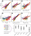 |
Fig. 9. Rmol scaling relations. The numbered panels show linear regression fits between log10ΣH2/ΣHI against six different physical quantities that we derived in Section 4: (1) Σgas, (2) ΣSFR, (3) Σ*, (4) Z′, (5) PDE, and (6) PDE/ΣSFR. Each color represents one galaxy. The lower right panel represents the range of correlation coefficient ρ and the mean absolute ρ for all galaxies for each individual fitted quantity shown in panels (1)–(6) using a hierarchical Bayesian method (linmix, see Section 4.9). All of the properties of the presented linear regression fits are listed in Table 5. |
We find for most of the galaxies moderate11 sublinear (i.e., β < 1) correlations between log10 Rmol and log10(x) (see Table 5 for an overview of correlation coefficient, slope, intercept, and their uncertainties, p-values, covariances and intrinsic scatters). We highlight a few notable exceptions to this general trend. For correlations between log10 Rmol and (i) log10 Σgas the galaxies NGCs 7496, 1566, and 1672 show a linear (i.e., β > 1) correlation, and NGC 1512 is the only galaxy that reveals a weak correlation with ρ = 0.12, (ii) log10 ΣSFR we find for NGC 1954 an exceptionally strong correlation (ρ = 0.97), and for NGC 5068 a negative correlation (ρ = −0.14), (iii) log10 Σ* the galaxy NGC 1566 shows a tight correlation (ρ = 0.85) with a perfectly linear slope (β = 1), (iv) log10 Z′ (rgal) all galaxies except NGC 5068 show a linear correlation, (v) PDE all galaxies except NGC 5068 show a tight correlation, (vi) PDE/ΣSFR we find weak correlations with the largest intrinsic scatter.
The bottom right panel in Figure 9 shows the ranges of ρ (black line) and the median ρ of all galaxies (grey circles), which we also indicate in Table 5 together with the covariance of the x and y-axis and fit parameters. We find the highest median ρ value for (i) PDE with ⟨ρ⟩ = 0.89 together with a high covariance and the smallest intrinsic scatter, followed by (ii) ΣSFR with ⟨ρ⟩ = 0.72, and (iii) Σgas with ⟨ρ⟩ = 0.67 together with the smallest intrinsic scatter but highest covariance compared to ΣSFR and PDE. We find the highest covariance for Rmol and ΣSFR/PDE (Cov(log10(x), log10(y)) = ∼20), followed by Rmol and PDE (Cov(log10(x), log10(y)) = ∼10; see Table 5). Looking at the covariances of the individual galaxies between Rmol and PDE or ΣSFR/PDE, it becomes apparent that NGC 1672 shows the highest covariance values (namely Cov(log10(x), log10(y)) = 13) for Rmol and PDE, and NGC 5068 (Cov(log10(x), log10(y)) = 25) for Rmol and ΣSFR/PDE.
6. Discussion
In this section, we discuss the physical drivers determining the balance between H I and H2 in our sample (i.e., the correlations shown in Figure 9). We further examine conditions at Rmol = 1, where above or below this transition, either H2 or H I dominates the cold ISM in nearby galaxies. We also investigate potential differences in physical quantities between interacting and non-interacting galaxies.
6.1. Dynamical equilibrium pressure PDE and Rmol
We find a tight, positive correlation between PDE and Rmol (with ⟨ρ⟩ = 0.89; see panel 5 of Figure 9 and Table 5), in line with many previous studies. For example, Wong & Blitz (2002) reported a strong correlation (with power-law indices of 0.8 and 0.92) between Rmol and the midplane hydrostatic pressure, mostly in a regime where ΣH2 > ΣHI. Blitz & Rosolowsky (2006) found similar results over three orders of magnitude in pressure for 14 galaxies. Leroy et al. (2008) showed that this relation also extends to the regime where H I dominates the ISM. However, they stated that the observed correlation between the midplane hydrostatic pressure and Rmol could be partly attributed to built-in covariance between the input quantities, as Σgas is one of the parameters used to calculate PDE (see Eq. (8)). Our estimated covariance of the fits in Table 5 between log10(Rmol) and log10(PDE) are in the range of ∼5 − 13, which are the highest among the shown quantities in Figure 9 (together with the ones for ΣSFR/PDE).
A study by Sun et al. (2020a) measured PDE values in the range of 103 − 106kB K cm−3 for 28 massive star-forming galaxies similar to our targets. This range is consistent with our PDE values of 102.5 − 107.5kB K cm−3, and only three galaxies overlap with their study. Sun et al. (2020a) found a moderate positive correlation between PDE and Rmol, with Spearman’s rank correlation coefficient of ρ = 0.58. With our better quality H I data, we see an even stronger (or tighter) correlation with ⟨ρ⟩ = 0.89 (i.e., the median over all the individual ρ for each galaxy, see Table 5 and Figure 9). This overall agrees with previous studies (Wong & Blitz 2002; Blitz & Rosolowsky 2006; Leroy et al. 2008) modulo different treatments for CO-to-H2 conversion factor, stellar mass-to-light ratio, and stellar disk geometry.
In the left panel of Figure 10, we show Rmol against PDE for our galaxies together with the aforementioned literature fits from Blitz & Rosolowsky 2006; Leroy et al. 2008; Sun et al. 2020a). The solid purple line shows a single ordinary least square (OLS) bisector fit12 calculated over all of our eight galaxies, which yields a slightly weaker relationship (with ρ = 0.4313, β = 0.98, α = −4.1, and p-value ≪0.001) compared to the median over all the individual ρ for each galaxy (i.e., ⟨ρ⟩ = 0.89, see Table 5).
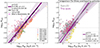 |
Fig. 10. Rmol against PDE. Left: shown here is an enlarged version of panel 5 from Figure 9, with the fit now performed over the entire sample (purple line) with the corresponding 3σ confidence interval (purple shaded region). The black, grey, and pink lines show literature fits adopted from Sun et al. (2020a), Leroy et al. (2008), and Blitz & Rosolowsky (2006), respectively. Right: Comparison between (i) Rmol and PDE estimates from Sun et al. (2020a) for three overlapping galaxies (grey markers) and (ii) our derived Rmol and PDE (colored markers). The different shapes of the markers correspond to different galaxies. |
In Sun et al. (2020a) the Rmol − PDE relation was shown for 28 galaxies, using older, less sensitive H I observations (mostly from literature VLA programs) to infer Rmol and PDE. Among these 28 galaxies, three overlap with our sample (NGC 1512, NGC 3511, and NGC 4535), allowing us to directly compare our Rmol and PDE measurements with theirs. Since we use the same datasets and assumptions for molecular gas and stellar mass components (i.e., ΣH2, σmol, ρ⋆ in Equation (8)), we can attribute all differences in PDE and Rmol to the different H I data entering our analyses.
In the right panel of Figure 10 we show a comparison of the two different estimates of Rmol and PDE, for the three overlapping galaxies NGC 1512, NGC 3511, and NGC 4535 with Sun et al. 2020a. We find that our derived Rmol (colored markers) are on average smaller than those found in Sun et al. (2020a) (grey markers); this is most obvious in the low-pressure regime. These differences can be attributed to several factors; their older H I observations reached lower sensitivities compared to our MeerKAT observations with an average rms of ∼0.3 mJy/beam over all of our galaxy maps (see Table 2). More importantly, their VLA data for these three galaxies reached coarser angular resolution of ∼30″ for NGC 3511, and NGC 4535 but ∼100″ for NGC 1512 compared to our new MeerKAT observations reaching angular resolutions of ∼15″. Sun et al. (2020a) measured ΣHI under the assumption of a smooth sub-beam flux distribution, driven by their limited resolution. With the higher quality data we now have available, it is clear that this assumption is not valid and we are now able to measure ΣHI at a resolution it is meant to be measured when using 1.5 kpc hexagon regions – at < 1.5 kpc (see Table 2). In Figure 11 we show a comparison of both of these datasets for NGC 1512. We find higher integrated intensities, thus higher ΣHI in the new observation, that causes Rmol to be lower than the Rmol measurements in Sun et al. (2020a). This causes the purple fit in the right panel of Figure 10 to be steeper than the one performed using the observations from Sun et al. (2020a). Given our comparisons of the three overlapping galaxies, we speculate that the fit by Sun et al. (2020a) might be even steeper with high-quality H I data.
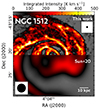 |
Fig. 11. Illustration of different data quality used in this work compared to data used in Sun et al. (2020a). The corresponding beam sizes of ∼15″ and ∼100″ are visible in the corners. |
6.2. Star formation surface density ΣSFR versus Rmol
The H2 mass fraction is linked to star formation as reflected by the Kennicutt–Schmidt (KS) relation (Schmidt 1959; Kennicutt 1998). Panel 2 of Figure 9 shows a moderate positive correlation of Rmol with the star formation rate surface density ΣSFR (with ⟨ρ⟩ = 0.67). We find covariances in the range of 1.90 − 4.90, slightly higher than for Σ* or Z′(rgal).
The observed correlation between ΣSFR and Rmol can be understood through their mutual correlation with PDE. We discuss the PDE vs. Rmol relation in the previous subsection; here we show an updated PDE vs. ΣSFR relation (incorporating our new, high-quality H I data) in Figure 12. Our observations support that PDE plays an important role in setting star formation. An additional factor is that in our sample H I surface densities lower than 8 M⊙ pc−2 contribute to a higher intrinsic scatter and shallower fit compared to the indicated literature fits. The gray dashed and dotted lines indicate the empirical scaling obtained from numerical simulations by Kim et al. (2013) and Ostriker & Kim (2022). The black line is drawn from observations by Sun et al. (2023) using 48 star forming spiral galaxies. If we would consider only regions of ΣHI > 8 M⊙ pc−2, then our fit would become as steep as the one shown in Kim et al. (2013) and Ostriker & Kim (2022). Recently it has been shown that galaxies with an offset to the star formation main sequence (SFMS) exhibit a nonlinear scaling relation between ΣSFR and PDE (see Ellison et al. 2024). Our and the Sun et al. (2023) galaxies are distributed along the SFMS and for those this pressure-regulated star formation theory seems to hold.
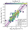 |
Fig. 12. ΣSFR against PDE colored by ΣHI. The purple line shows our fit over the entire sample with the corresponding 3σ confidence interval. The grey dashed and dotted lines show empirical scaling relations from Kim et al. (2013) and Ostriker & Kim (2022). The black dash-dotted line shows a fit from Sun et al. (2022). We see that low ΣHI is responsible for our shallower fit compared to the literature. |
We also examine whether there are galaxy-to-galaxy variations across the ΣSFR − PDE plane, and cross-check whether other quantities in our PDE estimation could contribute to the shallower relation (e.g ΣH2 or Σgas). We are unable to find significant galaxy-to-galaxy variations (see Figure D2). However, we do notice that the best-fit relation is shallow primarily due to a few low ΣHI measurements at PDE < 103 K cm−3 and > 106 K cm−3. The three low ΣHI measurements in the PDE > 106 K cm−3 regime are the central regions of NGC 1566, NGC 1672, and NGC 7496, where their AGN is responsible for a H I-depression. If we were to exclude these few data points, the majority of measurements are broadly consistent with steeper slopes.
6.3. Other quantities and Rmol
In the past, it has been shown that the H I-to-H2 transition depends on the total gas surface density and metallicity in a PDR (e.g., Sternberg 1988), assuming a spherical cloud that is surrounded by a uniform and isotropic interstellar radiation field (e.g., Krumholz et al. 2009; Krumholz & Burkert 2010). Krumholz & Burkert (2010) studied the steady-state equilibration and photodissociation of H2 and assumed the H I-to-H2 transition to be infinitely sharp and suggested that in a given ISM environment (i.e., at fixed metallicity) the total gas surface density determines the transition of gas phases (also tested with observations e.g. Fumagalli et al. 2010; Lee et al. 2012; or compared with 1D semi-analytical models e.g. Sternberg et al. 2014). Panel 1 and panel 4 in Figure 9 show that the observationally derived Rmol does moderately correlate with the total gas surface density Σgas (with ⟨ρ⟩ = 0.67) and show a weak to moderate correlation with metallicity Z′(rgal) (with ⟨ρ⟩ = 0.48). The covariances of each of the galaxies (shown in Table 5) of these fits are between −0.74 and 0.90, which indicates that the relationship is not strongly pronounced.
Looking at individual galaxies, we find ‘outliers’ that are responsible for the wide ranges of ρ values for Σgas, ΣSFR, Σ*, and Z′(rgal). However, there is no one specific galaxy that appears to be an outlier in all of the aforementioned quantities. NGC 1512 is responsible for the wide ranges of ρ values for Σgas, that is H I-dominated at low Σgas regimes. NGC 5068 seems to show different slopes and exhibits negative ρ values in Rmol versus ΣSFR, Σ*, and Z′(rgal). This can be attributed to the relatively weak CO emission from this target and consequently the low S/N of the PHANGS-ALMA CO map. This low S/N could introduce biases in measuring Rmol and could explain the different behavior seen in the fits. Additionally, the CO map only covers a fraction of the optical disk of NGC 5068, which highlights that additional observations are needed to fully understand this behavior. IC 1954 shows a shallow fit between Rmol and Σ* because of significant Rmol measurements in the low Σ* regime. These two galaxies (NGC 5068 and IC 1954) are also those with the lowest total stellar mass (M⋆) in our sample (see Table 1). We expect an increase in Rmol with  . Panel 6 in Figure 9 shows globally this behavior for most of our galaxies. However, three galaxies, NGC 7496, NGC 5068, and IC 1954, show the opposite trend. We note that the galaxies NGC 5068 and IC 1954 are according to Figure 8 H I-dominated. However, NGC 7496 is quite the contrary. We can not attribute a specific reason why this galaxy shows this opposite trend. However, the overall trend of increasing ΣH2 with
  holds for our sample of star forming spiral galaxies.
6.4. Differences between interacting and noninteracting galaxies?
Figure 2 shows a prominent example of an interacting galaxy – NGC 1512 interacting with NGC 1510. In our sample, we have another galaxy that is potentially interacting with a close-by companion: NGC 3511 with NGC 3513 (see Figure 3). Apart from these two galaxies none of the others appear to be interacting14. Gas can generally be stripped from a companion, or it can flow inwards because of the torque exerted by the companion or the asymmetric structure created by the interaction. The exchange of gas in different phases can increase the reservoir of molecular gas and replenish the atomic gas by cooling (see e.g. Moreno et al. 2019).
Blitz & Rosolowsky (2006) observed a different behavior in Rmol vs. pressure between interacting and non-interacting galaxies. From a global view, Lisenfeld et al. (2019) found that mergers have a larger molecular mass gas fraction than their isolated counterparts, resulting in accelerated atomic to molecular gas conversion (Kaneko et al. 2017). More recent studies show evidence that environmental processes, potentially due to interactions, are linked to quenching in H I-poor galaxies. This simultaneously reduces the molecular gas surface density and star formation efficiency compared to regions in H I-normal systems (see e.g. Villanueva et al. 2022; Jiménez-Donaire et al. 2023; Brown et al. 2023). On the contrary, in galaxy clusters environmental processes can lead to an increase in Rmol (see e.g. Moretti et al. 2023). The question arises now whether we find different signatures in PDE, in Rmol, or other physical quantities in these two galaxies compared to the other six.
What both interacting galaxies have in common are their relatively low global values in star formation rate ∼0.1 log(M⊙ yr−1) (see Table 1) among our sample. In the right panel of Figure 8, which shows Rmol versus rgal/r25 for individual galaxies, it is evident that NGC 1512 (pink markers and line) shows the smallest radius of where molecular gas becomes dominant rgal = 0.23 r25. However, NGC 3511 (yellow markers and line) never crosses the Rmol = 1 equilibrium and, hence is H I-dominated. The first panel in Figure 9 and their corresponding intrinsic scatter values listed in Table 5, show that NGC 1512 and NGC 3511 have the highest intrinsic scatter in our sample, namely 0.23 and 0.10 dex, respectively. The second panel in Figure 9 – Rmol against ΣSFR – does not show a particularly different behavior for NGC 1512 and NGC 3511 as compared to the other galaxies in our sample. This also holds for the physical quantities Σ*, Z′, and ΣSFRPDE. The fifth panel in Figure 9 shows that measurements of Rmol against PDE for NGC 1512 have the highest intrinsic scatter in our sample of 0.10 dex (also see Figure D2). However, our sample of a total of eight galaxies, of which only two are interacting, is not statistically significant, and so it is unclear whether galaxy interactions meaningfully impact the Rmol relations we are investigating.
6.5. Atomic versus molecular dominated ISM
In spiral galaxies, the transition between a H I-dominated and a predominantly H2-dominated ISM takes place at a characteristic value for most quantities. In Table 6 we list the conditions at Rmol = 1 and compare our measured values to the ones in Leroy et al. (2008). For each galaxy, we measured the median of the quantity in question over all hexagonal apertures where ΣH2 ≈ 0.8 − 1.2 ΣHI. We show the median transition value along with the 1σ scatter among our galaxies. At Rmol = 1 the baryon mass budget is dominated by stars Σ* ≈ 78 M⊙ pc−2 while the total gas surface density is Σgas ≈ 14 M⊙ pc−2. The dynamical equilibrium pressure corresponds to 2.9 × 104 kB K cm−3. We note that some of these values are different from those quoted in Table 6 taken from Leroy et al. (2008), but the mean values overlap within the scatter, and since these quantities depend on the galaxy’s properties, a perfect match is not necessarily to be expected.
Conditions at Rmol = 1, where ΣHI ≈ ΣH2.
In the right panel of Figure 8 and in Table 4 we found that three galaxies never cross the Rmol equilibrium border to enter the molecular gas dominated regime (i.e. Rmol > 1). These H I-dominated galaxies are NGC 3511, NGC 5068, and IC 1954. NGC 5068, and IC 1954 are the lowest M⋆ galaxies in our sample with M⋆ = 9.4 log(M⊙) and M⋆ = 9.7 log(M⊙), respectively. We note that this shows that it is important to study each galaxy individually, as they show different behaviors in Rmol under different local conditions (see also Section 6.3). However, we also believe that listing the scaling relation across all galaxies, similar to what we did for Rmol versus rgal/r25 in Figure 8 and Eq. (16), may be useful for future comparisons, and therefore we list them in Table 7.
Scaling relation across all galaxies.
7. Conclusion
We used a multiwavelength approach including new observations of eight nearby galaxies taken with the MeerKAT telescope (PHANGS-MeerKAT, this work + MHONGOOSE from de Blok et al. 2016). In this work, we analyzed at what galactocentric radii atomic gas becomes more dominant compared to molecular gas and examined local conditions in individual galaxies and how they correlate with the molecular gas fraction Rmol = ΣH2/ΣHI. We performed our analysis in a way that we averaged each quantity (ΣH2, ΣHI, Σgas, ΣSFR, Σ*, Z′(rgal), PDE, and ΣSFR/¶DE) over 1.5 kpc hexagonal regions (following Sun et al. 2022). We find the following results:
-
1)
We presented new MeerKAT H I observations of three nearby spiral galaxies NGC 1512, NGC 4535, and NGC 7496 (PHANGS-MeerKAT) at 15″ angular resolution, which we combined with additional observations towards five nearby galaxies IC1954, NGC 1566, NGC 1672, NGC 3511, and NGC 5068 (from MHONGOOSE); see Figures 1–3. Their H I distribution shows gigantic spiral arms (in NGC 1512, NGC 1566, and NGC 4535), splitting into sub-arms (in NGC 1512), compact disks (in NGC 3511 and IC 1954), ring-like structures (in NGC 7496 and a smaller one in NGC 1512), or additional clumps (in NGC 1512 and NGC 1566).
-
2)
We detected on average significant H I emission out to a radius of ∼50 kpc (see Figures 5, 6, and 7), which is ∼5 times the 3σ detected CO emission (see Table 3). In terms of rH I, defined as the ΣHI = 1 M⊙ pc−2 isophote, we found an average rHI of ∼22 kpc, which is ∼2 times r25 (with ranges of 1 − 3 times r25) and ≈6 times reff.
-
3)
The Rmol − rgal/r25 fit crosses the Rmol = 1 border (where ΣHI ≈ ΣH2, indicated as a grey horizontal line in Figure 8) at rgal ∼ 0.4 r25. This means that molecular gas is more dominant at 0 − 0.4 optical radii, and atomic gas becomes more dominant at rgal > 0.4 optical radii.
-
4)
To understand how Rmol responds to the local conditions in each galaxy, we investigated scaling relations with various physical parameters using a hierarchical Bayesian method to include uncertainties and upper limits (see Section 4.9). Among all of these fits Rmol − PDE shows the tightest correlation with a median correlation coefficient ρ of each galaxy’s ρ of ⟨ρ⟩ = 0.89, together with the smallest intrinsic scatter (∼0.1 dex; see Figure 9 and Table 5).
-
5)
A positive correlation between Rmol and PDE has been found in previous studies (e.g., Blitz & Rosolowsky 2004; Leroy et al. 2008; Sun et al. 2020b). Similar to these studies we performed a OLS bisector fit over all galaxies, which yields for our sample a correlation with ρ = 0.43 (see Figure 10). We attribute the differences in our Rmol measurements compared to previous studies to the improved resolution and sensitivity of our H I data. Upcoming observations will increase the sample size and thus allow for further investigation.
-
6)
We investigated how the dynamical equilibrium pressure corresponds to the star formation rate. We found that ΣHI measurements lower than 8 M⊙ pc−2 are responsible for a shallower fit (see Figure 12) compared to the empirical scaling relations from Kim et al. (2013), Ostriker & Kim (2022) but agree with the observational one by Sun et al. (2023).
-
7)
In our sample, NGC 1512 interacts with NGC 1510 and potentially NGC 3511 with its close-by companion NGC 3513. We did not find a significantly different behavior than the non- interacting galaxies in our sample among all of our physical quantities.
-
8)
We found that the transition between an H I-dominated and H2-dominated ISM takes place at a characteristic value for most quantities we measured. For example, at Rmol = 1 the baryon mass budget is dominated by stars Σ* > 5 Σgas (i.e. Σ* ≈ 78 M⊙ pc−2 while the total gas is Σgas ≈ 14 M⊙ pc−2; see Table 6).
With upcoming MeerKAT and/or high-resolution VLA H I observations of additional nearby galaxies targeted by the PHANGS and/or MHONGOOSE projects that have multiwavelength data available15, a natural next step is to perform this analysis on a larger sample. With these fantastic wide-field H I surveys, wider CO mapping would also extend these relations into the outer disk environments (a first step towards this goal has been taken within PHANGS; observing CO(1–0) towards 10 galaxies with ALMA’s compact array, PI: A. Leroy). This will allow us to further investigate how global galaxy properties (stellar mass, star formation rate, or morphology) impact the conversion from atomic to molecular gas in nearby galaxies (D < 20 Mpc or z < 0.005).
The dense gas fraction, fdense, is traced by the integrated intensity of HCN(1–0) over CO and has been found to correlate with Rmol (e.g., Usero et al. 2015).
These are the 8 × frequency-averaged 32K data.
We roughly measure the length of a spiral arm as 30′ long which translates at NGC 1512’s distance of 18.8 Mpc to ∼160 kpc.
We chose 1.5 kpc sized hexagonal apertures because 1.5 kpc represents one linear resolution element of our H I observations. 1.5 kpc is also the best common resolution achievable for all galaxies in our sample.
We note that this Z-based prescription overall matches with the velocity dispersion prescription derived by Teng et al. (2024), although the former has a ∼3× larger uncertainty. Additionally, the αCO(1 − 0) is likely to be overestimated in the centers of the galaxies with the Z′-based prescription. Our central regions are 1.5 kpc in size and most of this effect would most likely be averaged out. To be able to compare with literature trends, we decided to use the Z′-based prescription.
Here we refer to a “moderate” correlation if the correlation coefficient ρ lies in the range of 0.5 − 0.7 and a “tight” correlation if ρ > 0.7.
We use here and in the following sections the OLS bisector method in logarithmic space (see Isobe et al. 1990, for more details) to better compare to studies by Leroy et al. (2008) and Sun et al. (2020a) who used the same method.
The correlation coefficients given here and in the following sections are Spearman rank correlation coefficients, which are suited better for a comparison with the literature than the Pearson correlation coefficient using linmix.
We note that there are three other galaxies in the field of view of NGC 7496, see Appendix E. In this paper, we consider them to be non-interacting galaxies, as they show no signs of bridges or tails indicating interaction. However, this may also be a matter of sensitivity, where we are unable to capture this highly diffuse H I gas. Throughout the discussion, we have kept an eye on NGC 7496 to see whether or not it follows a particular trend associated with the two interacting galaxies in our sample. Additionally, we note that NGC 4535 is a member of the Virgo Cluster of galaxies.
Acknowledgments
CE gratefully acknowledges funding from the Deutsche Forschungsgemeinschaft (DFG) Sachbeihilfe, grant number BI1546/3-1. CE acknowledges funding from the European Research Council (ERC) under the European Union’s Horizon 2020 research and innovation program (grant agreement No.726384/Empire). JS acknowledges support by the National Aeronautics and Space Administration (NASA) through the NASA Hubble Fellowship grant HST-HF2-51544 awarded by the Space Telescope Science Institute (STScI), which is operated by the Association of Universities for Research in Astronomy, Inc., under contract NAS 5-26555. The work of AKL is partially supported by the National Science Foundation under Grants No. 1615105, 1615109, and 1653300. WJGdB, FMM, and JH acknowledge funding from the European Research Council (ERC) under the European Union’s Horizon 2020 research and innovation programme (grant agreement No. 882793 “MeerGas”). M.C. gratefully acknowledges funding from the DFG through an Emmy Noether Research Group (grant number CH2137/1-1). COOL Research DAO is a Decentralized Autonomous Organization supporting research in astrophysics aimed at uncovering our cosmic origins. RSK acknowledges funding from the European Research Council via the ERC Synergy Grant “ECOGAL” (project ID 855130), from the German Excellence Strategy via the Heidelberg Cluster of Excellence (EXC 2181 - 390900948) “STRUCTURES”, and from the German Ministry for Economic Affairs and Climate Action in project “MAINN” (funding ID 50OO2206). He also thanks for computing resources provided by The Länd and DFG through grant INST 35/1134-1 FUGG and for data storage at SDS@hd through grant INST 35/1314-1 FUGG. HAP acknowledges support from the National Science and Technology Council of Taiwan under grant 110-2112-M-032-020-MY3. AU acknowledges support from the Spanish grants PID2019-108765GB-I00, funded by MCIN/AEI/10.13039/501100011033, and PID2022-138560NB-I00, funded by MCIN/AEI/10.13039/501100011033/FEDER, EU. ER acknowledges the support of the Natural Sciences and Engineering Research Council of Canada (NSERC), funding reference number RGPIN-2022-03499. DJP and SK greatly acknowledge support from the South African Research Chairs Initiative of the Department of Science and Technology and National Research Foundation. This paper makes use of MeerKAT observations. The MeerKAT telescope is operated by the South African Radio Astronomy Observatory, which is a facility of the National Research Foundation, an agency of the Department of Science and Innovation. This paper makes use of the following ALMA data, which have been processed as part of the PHANGS–ALMA CO(2–1) survey: ADS/JAO.ALMA#2015.1.00925.S, ADS/JAO.ALMA#2015.1.00956.S, ADS/JAO.ALMA#2017.1.00392.S, ADS/JAO.ALMA#2017.1.00886.L, ADS/JAO.ALMA#2018.1.01651.S. ADS/JAO.ALMA#2018.A.00062.S. ALMA is a partnership of ESO (representing its member states), NSF (USA), and NINS (Japan), together with NRC (Canada), MOST and ASIAA (Taiwan), and KASI (Republic of Korea), in cooperation with the Republic of Chile. The Joint ALMA Observatory is operated by ESO, AUI/NRAO, and NAO. Figure 1 in this paper uses hips2fits, (https://alasky.cds.unistra.fr/hips-image-services/hips2fits) a service provided by CDS.
References
- Accurso, G., Saintonge, A., Catinella, B., et al. 2017, MNRAS, 470, 4750 [NASA ADS] [Google Scholar]
- Allen, R. J., Knapen, J. H., Bohlin, R., & Stecher, T. P. 1997, ApJ, 487, 171 [NASA ADS] [CrossRef] [Google Scholar]
- Alloin, D., Pelat, D., Phillips, M., & Whittle, M. 1985, ApJ, 288, 205 [NASA ADS] [CrossRef] [Google Scholar]
- Anand, G. S., Lee, J. C., Van Dyk, S. D., et al. 2021, MNRAS, 501, 3621 [Google Scholar]
- Barnes, A. T., Chandar, R., Kreckel, K., et al. 2022, A&A, 662, L6 [NASA ADS] [CrossRef] [EDP Sciences] [Google Scholar]
- Belfiore, F., Leroy, A. K., Sun, J., et al. 2023, A&A, 670, A67 [NASA ADS] [CrossRef] [EDP Sciences] [Google Scholar]
- Bellhouse, C., McGee, S. L., Smith, R., et al. 2021, MNRAS, 500, 1285 [Google Scholar]
- Bigiel, F., Leroy, A., Walter, F., et al. 2008, AJ, 136, 2846 [NASA ADS] [CrossRef] [Google Scholar]
- Blitz, L., & Rosolowsky, E. 2004, ApJ, 612, L29 [NASA ADS] [CrossRef] [Google Scholar]
- Blitz, L., & Rosolowsky, E. 2006, ApJ, 650, 933 [NASA ADS] [CrossRef] [Google Scholar]
- Boselli, A., Serra, P., de Gasperin, F., et al. 2023, A&A, 676, A92 [NASA ADS] [CrossRef] [EDP Sciences] [Google Scholar]
- Braine, J., Ferguson, A. M. N., Bertoldi, F., & Wilson, C. D. 2007, ApJ, 669, L73 [NASA ADS] [CrossRef] [Google Scholar]
- Brown, T., Roberts, I. D., Thorp, M., et al. 2023, ApJ, 956, 37 [NASA ADS] [CrossRef] [Google Scholar]
- Chabrier, G. 2003, PASP, 115, 763 [Google Scholar]
- Chevance, M., Krumholz, M. R., McLeod, A. F., et al. 2023, ASP Conf. Ser., 534, 1 [NASA ADS] [Google Scholar]
- Collier, J. D., Frank, B., Sekhar, S., & Taylor, A. R. 2021, 2021 XXXIVth General Assembly and Scientific Symposium of the International Union of Radio Science (URSI GASS), 1 [Google Scholar]
- Combes, F., García-Burillo, S., Casasola, V., et al. 2014, A&A, 565, A97 [NASA ADS] [CrossRef] [EDP Sciences] [Google Scholar]
- de Blok, W. J. G., Adams, E. A. K., Amram, P., et al. 2016, MeerKAT Science: On the Pathway to the SKA, 7 [Google Scholar]
- de Blok, W. J. G., Healy, J., Maccagni, F. M., et al. 2024, A&A, 688, A109 [NASA ADS] [CrossRef] [EDP Sciences] [Google Scholar]
- den Brok, J. S., Chatzigiannakis, D., Bigiel, F., et al. 2021, MNRAS, 504, 3221 [NASA ADS] [CrossRef] [Google Scholar]
- de Vaucouleurs, G., de Vaucouleurs, A., Corwin, Jr., H. G., et al. 1991, Third Reference Catalogue of Bright Galaxies [Google Scholar]
- De Vis, P., Jones, A., Viaene, S., et al. 2019, A&A, 623, A5 [NASA ADS] [CrossRef] [EDP Sciences] [Google Scholar]
- Dobbs, C. L., Krumholz, M. R., Ballesteros-Paredes, J., et al. 2014, in Protostars and Planets VI, eds. H. Beuther, R. S. Klessen, C. P. Dullemond, & T. Henning, 3 [Google Scholar]
- Eibensteiner, C., Bigiel, F., Leroy, A. K., et al. 2023, A&A, 675, A37 [NASA ADS] [CrossRef] [EDP Sciences] [Google Scholar]
- Ellison, S. L., Pan, H.-A., Bluck, A. F. L., et al. 2024, MNRAS, 527, 10201 [Google Scholar]
- Elmegreen, B. G. 1989, ApJ, 338, 178 [NASA ADS] [CrossRef] [Google Scholar]
- Elmegreen, B. G. 1993, ApJ, 411, 170 [NASA ADS] [CrossRef] [Google Scholar]
- Elson, E., Głowacki, M., Deane, R., Isaacs, N., & Ndaliso, X. 2023, ArXiv e-prints [arXiv:2309.02076] [Google Scholar]
- Emsellem, E., Schinnerer, E., Santoro, F., et al. 2022, A&A, 659, A191 [NASA ADS] [CrossRef] [EDP Sciences] [Google Scholar]
- Fumagalli, M., Krumholz, M. R., & Hunt, L. K. 2010, ApJ, 722, 919 [NASA ADS] [CrossRef] [Google Scholar]
- Girichidis, P., Offner, S. S. R., Kritsuk, A. G., et al. 2020, Space Sci. Rev., 216, 68 [NASA ADS] [CrossRef] [Google Scholar]
- Glover, S. C. O., & Clark, P. C. 2012, MNRAS, 421, 9 [NASA ADS] [Google Scholar]
- Gong, M., Ostriker, E. C., & Kim, C.-G. 2018, ApJ, 858, 16 [Google Scholar]
- Groves, B., Kreckel, K., Santoro, F., et al. 2023, MNRAS, 520, 4902 [Google Scholar]
- Healy, J., de Blok, W. J. G., Maccagni, F. M., et al. 2024, A&A, 687, A254 [NASA ADS] [CrossRef] [EDP Sciences] [Google Scholar]
- Heiner, J. S., Allen, R. J., & van der Kruit, P. C. 2011, MNRAS, 416, 2 [NASA ADS] [Google Scholar]
- Hollenbach, D. J., & Tielens, A. G. G. M. 1999, Rev. Mod. Phys., 71, 173 [Google Scholar]
- Isobe, T., Feigelson, E. D., Akritas, M. G., & Babu, G. J. 1990, ApJ, 364, 104 [Google Scholar]
- Jenkins, L. P., Brandt, W. N., Colbert, E. J. M., et al. 2011, ApJ, 734, 33 [NASA ADS] [CrossRef] [Google Scholar]
- Jiménez-Donaire, M. J., Bigiel, F., Leroy, A. K., et al. 2019, ApJ, 880, 127 [CrossRef] [Google Scholar]
- Jiménez-Donaire, M. J., Brown, T., Wilson, C. D., et al. 2023, A&A, 671, A3 [NASA ADS] [CrossRef] [EDP Sciences] [Google Scholar]
- Jonas, J., & MeerKAT Team 2016, MeerKAT Science: On the Pathway to the SKA, 1 [Google Scholar]
- Kaneko, H., Kuno, N., Iono, D., et al. 2017, PASJ, 69, 66 [NASA ADS] [CrossRef] [Google Scholar]
- Kelly, B. C. 2007, ApJ, 665, 1489 [Google Scholar]
- Kennicutt, R. C., Jr 1998, ApJ, 498, 541 [Google Scholar]
- Kewley, L. J., & Ellison, S. L. 2008, ApJ, 681, 1183 [Google Scholar]
- Kim, C.-G., Kim, W.-T., & Ostriker, E. C. 2011, ApJ, 743, 25 [NASA ADS] [CrossRef] [Google Scholar]
- Kim, C.-G., Ostriker, E. C., & Kim, W.-T. 2013, ApJ, 776, 1 [NASA ADS] [CrossRef] [Google Scholar]
- Klessen, R. S., & Glover, S. C. O. 2016, in Saas-Fee Advanced Course, eds. Y. Revaz, P. Jablonka, R. Teyssier, & L. Mayer, 43, 85 [NASA ADS] [CrossRef] [Google Scholar]
- Koda, J., Watson, L., Combes, F., et al. 2022, ApJ, 941, 3 [NASA ADS] [CrossRef] [Google Scholar]
- Koribalski, B. S., & López-Sánchez, Á. R. 2009, MNRAS, 400, 1749 [NASA ADS] [CrossRef] [Google Scholar]
- Kreckel, K., Ho, I.-T., Blanc, G., et al. 2019, ApJ, 887, 80 [NASA ADS] [CrossRef] [Google Scholar]
- Krumholz, M., & Burkert, A. 2010, ApJ, 724, 895 [NASA ADS] [CrossRef] [Google Scholar]
- Krumholz, M. R., McKee, C. F., & Tumlinson, J. 2009, ApJ, 693, 216 [NASA ADS] [CrossRef] [Google Scholar]
- Lang, P., Meidt, S. E., Rosolowsky, E., et al. 2020, ApJ, 897, 122 [CrossRef] [Google Scholar]
- Laudage, S., Eibensteiner, C., Bigiel, F., et al. 2024, A&A, 690, A169 [NASA ADS] [CrossRef] [EDP Sciences] [Google Scholar]
- Lee, M.-Y., Stanimirović, S., Douglas, K. A., et al. 2012, ApJ, 748, 75 [NASA ADS] [CrossRef] [Google Scholar]
- Leroy, A. K., Walter, F., Brinks, E., et al. 2008, AJ, 136, 2782 [Google Scholar]
- Leroy, A. K., Sandstrom, K. M., Lang, D., et al. 2019, ApJS, 244, 24 [Google Scholar]
- Leroy, A. K., Hughes, A., Liu, D., et al. 2021a, ApJS, 255, 19 [NASA ADS] [CrossRef] [Google Scholar]
- Leroy, A. K., Schinnerer, E., Hughes, A., et al. 2021b, ApJS, 257, 43 [NASA ADS] [CrossRef] [Google Scholar]
- Leroy, A. K., Rosolowsky, E., Usero, A., et al. 2022, ApJ, 927, 149 [NASA ADS] [CrossRef] [Google Scholar]
- Lisenfeld, U., Xu, C. K., Gao, Y., et al. 2019, A&A, 627, A107 [NASA ADS] [CrossRef] [EDP Sciences] [Google Scholar]
- Maccagni, F. M., & de Blok, W. J. G. 2024 arXiv e-prints [arXiv:2407.03166] [Google Scholar]
- Mac Low, M.-M., & Glover, S. C. O. 2012, ApJ, 746, 135 [NASA ADS] [CrossRef] [Google Scholar]
- Mac Low, M.-M., & Klessen, R. S. 2004, Rev. Mod. Phys., 76, 125 [Google Scholar]
- Makarov, D., Prugniel, P., Terekhova, N., Courtois, H., & Vauglin, I. 2014, A&A, 570, A13 [NASA ADS] [CrossRef] [EDP Sciences] [Google Scholar]
- Malkan, M. A., Gorjian, V., & Tam, R. 1998, ApJS, 117, 25 [Google Scholar]
- Martin, D. C., Fanson, J., Schiminovich, D., et al. 2005, ApJ, 619, L1 [Google Scholar]
- McKee, C. F., & Ostriker, E. C. 2007, ARA&A, 45, 565 [Google Scholar]
- Moreno, J., Torrey, P., Ellison, S. L., et al. 2019, MNRAS, 485, 1320 [NASA ADS] [CrossRef] [Google Scholar]
- Moretti, A., Serra, P., Bacchini, C., et al. 2023, ApJ, 955, 153 [NASA ADS] [CrossRef] [Google Scholar]
- Offringa, A. R., McKinley, B., Hurley-Walker, N., et al. 2014, MNRAS, 444, 606 [Google Scholar]
- Ostriker, E. C., & Kim, C.-G. 2022, ApJ, 936, 137 [NASA ADS] [CrossRef] [Google Scholar]
- Ostriker, E. C., McKee, C. F., & Leroy, A. K. 2010, ApJ, 721, 975 [CrossRef] [Google Scholar]
- Pettini, M., & Pagel, B. E. J. 2004, MNRAS, 348, L59 [NASA ADS] [CrossRef] [Google Scholar]
- Pilyugin, L. S., & Grebel, E. K. 2016, MNRAS, 457, 3678 [NASA ADS] [CrossRef] [Google Scholar]
- Rosolowsky, E., Hughes, A., Leroy, A. K., et al. 2021, MNRAS, 502, 1218 [NASA ADS] [CrossRef] [Google Scholar]
- Saintonge, A., & Catinella, B. 2022, ARA&A, 60, 319 [NASA ADS] [CrossRef] [Google Scholar]
- Salim, S., Boquien, M., & Lee, J. C. 2018, ApJ, 859, 11 [Google Scholar]
- Salo, H., Laurikainen, E., Laine, J., et al. 2015, ApJS, 219, 4 [Google Scholar]
- Sánchez, S. F., Rosales-Ortega, F. F., Iglesias-Páramo, J., et al. 2014, A&A, 563, A49 [CrossRef] [EDP Sciences] [Google Scholar]
- Sánchez, S. F., Barrera-Ballesteros, J. K., López-Cobá, C., et al. 2019, MNRAS, 484, 3042 [CrossRef] [Google Scholar]
- Schmidt, M. 1959, ApJ, 129, 243 [NASA ADS] [CrossRef] [Google Scholar]
- Schruba, A., Leroy, A. K., Walter, F., et al. 2011, AJ, 142, 37 [NASA ADS] [CrossRef] [Google Scholar]
- Schruba, A., Bialy, S., & Sternberg, A. 2018, ApJ, 862, 110 [NASA ADS] [CrossRef] [Google Scholar]
- Serra, P., Maccagni, F. M., Kleiner, D., et al. 2019, A&A, 628, A122 [NASA ADS] [CrossRef] [EDP Sciences] [Google Scholar]
- Serra, P., Maccagni, F. M., Kleiner, D., et al. 2023, A&A, 673, A146 [NASA ADS] [CrossRef] [EDP Sciences] [Google Scholar]
- Sheth, K., Regan, M., Hinz, J. L., et al. 2010, PASP, 122, 1397 [Google Scholar]
- Smith, R. J., Glover, S. C. O., Clark, P. C., Klessen, R. S., & Springel, V. 2014, MNRAS, 441, 1628 [NASA ADS] [CrossRef] [Google Scholar]
- Spitzer, L., Jr 1942, ApJ, 95, 329 [NASA ADS] [CrossRef] [Google Scholar]
- Sternberg, A. 1988, ApJ, 332, 400 [NASA ADS] [CrossRef] [Google Scholar]
- Sternberg, A., Le Petit, F., Roueff, E., & Le Bourlot, J. 2014, ApJ, 790, 10 [CrossRef] [Google Scholar]
- Sternberg, A., Bialy, S., & Gurman, A. 2024, ApJ, 960, 8 [NASA ADS] [CrossRef] [Google Scholar]
- Sun, J., Leroy, A. K., Schruba, A., et al. 2018, ApJ, 860, 172 [NASA ADS] [CrossRef] [Google Scholar]
- Sun, J., Leroy, A. K., Ostriker, E. C., et al. 2020a, ApJ, 892, 148 [NASA ADS] [CrossRef] [Google Scholar]
- Sun, J., Leroy, A. K., Schinnerer, E., et al. 2020b, ApJ, 901, L8 [NASA ADS] [CrossRef] [Google Scholar]
- Sun, J., Leroy, A. K., Rosolowsky, E., et al. 2022, AJ, 164, 43 [NASA ADS] [CrossRef] [Google Scholar]
- Sun, J., Leroy, A. K., Ostriker, E. C., et al. 2023, ApJ, 945, L19 [NASA ADS] [CrossRef] [Google Scholar]
- Tamburro, D., Rix, H. W., Leroy, A. K., et al. 2009, AJ, 137, 4424 [Google Scholar]
- Teng, Y.-H., Chiang, I. D., Sandstrom, K. M., et al. 2024, ApJ, 961, 42 [NASA ADS] [CrossRef] [Google Scholar]
- Usero, A., Leroy, A. K., Walter, F., et al. 2015, AJ, 150, 115 [Google Scholar]
- Villanueva, V., Bolatto, A. D., Vogel, S., et al. 2022, ApJ, 940, 176 [NASA ADS] [CrossRef] [Google Scholar]
- Wang, J., Koribalski, B. S., Serra, P., et al. 2016, MNRAS, 460, 2143 [Google Scholar]
- Westmeier, T., Kitaeff, S., Pallot, D., et al. 2021, MNRAS, 506, 3962 [NASA ADS] [CrossRef] [Google Scholar]
- Wolfire, M. G., Hollenbach, D., & McKee, C. F. 2010, ApJ, 716, 1191 [Google Scholar]
- Wong, T., & Blitz, L. 2002, ApJ, 569, 157 [CrossRef] [Google Scholar]
- Wright, E. L., Eisenhardt, P. R. M., Mainzer, A. K., et al. 2010, AJ, 140, 1868 [Google Scholar]
Appendix A: Star formation rate surface density
In this section, we compare two different methods for computing the star formation rate surface density ΣSFR. We recall that in the main part of this work, we used the maps based on a combination of FUV and mid-IR emission, since these observations are available for all galaxies in our study (see Section 4.4). Extinction-corrected Hα-based SFR measurements together with the new calibration by Belfiore et al. (2023) are considered to be one of the most reliable SFR measurements. However, the required MUSE data from the PHANGS-MUSE sample (see Emsellem et al. 2022) are available for only 5 out of 8 of the galaxies studied in this work (see Table A.1). We examine here the reliability of the Rmol versus ΣSFR fit (shown in Figure 9 second panel) by comparing it to the Hα-based SFR in the 5 galaxies where both SFR measurements are available. Figure A.1 shows that the relation using the Hα-based ΣSFR shows a similar trend but with less scatter and thus might be indicative of a tighter relationship between Rmol and ΣSFR.
PHANGS-MUSE coverage of our sample.
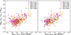 |
Fig. A.1. Comparison of star formation rate surface densities using FUV+WISE4-based and the Hα-based measurements in the Rmol - ΣSFR plane. |
Appendix B: Metallicity
In this section, we compare two different approaches to estimate the metallicity. We recall that in the paper we used scaling relations to get general metallicity trends assuming a global galaxy mass-metallicity relation and a fixed radial metallicity gradient within each galaxy (see Section 4.8). In this section, we compare this approach with the use of metallicity measurements of individual HII regions for the galaxies in the PHANGS-MUSE sample (see Table A.1). They have been derived in Groves et al. (2023) as the mean HII region metallicity relative to solar using the PG16S calibration (see also Kreckel et al. 2019) that is defined in Pilyugin & Grebel (2016). This prescription is based on a calibration against a sample of a few hundred HII regions where direct auroral line detections were used to calculate the electron temperature (see Groves et al. 2023, for more details). Figure B.1 shows that comparison (not normalized to the solar metallicity, as we did in the main part of the paper), and it is immediately apparent the majority of galaxies is "moved" to lower metallicity measurements – ∼0.2 dex lower Z(HII),PG16S compared to Z(rgal),O3N2. Differences in individual HII region metallicities based on different measurement approaches have been reported to differ up to 0.7 dex in 12+log(O/H) for the same HII regions (Kewley & Ellison 2008). To check the variations of these two calibration methods we used the third panel of Figure B1 in the Appendix of De Vis et al. (2019) that compares these calibration methods. We use a linear fit of the form of y = 1.1 * x − 0.65 and limit to relevant metallicity ranges to "convert" (denoted as ( * )) our Z(HII),PG16S to Z(HII),O3N2( * ). We find ∼0.2 dex difference between Z(HII),PG16S and Z(HII),O3N2( * ), consistent with the difference aforementioned. One galaxy – NGC 5068 (green quared markers) – is in both measurements distinct from the other galaxies: it is more metal-poor. Neglecting NGC 5068 at Rmol = 1 reveals that Z(HII),PG16S ≈ 8.55 and Z(HII),O3N2( * ) ≈ 8.75. The galaxy NGC 7496 appears according to the Z(rgal),O3N2 measurements more metal-poor compared to the Z(HII),PG16S and Z(HII),O3N2( * ) measurements.
Overall both of the calibrations generally yield similar metallicity gradients, just with an offset in the normalization (see e.g. Figure 20 in Kreckel et al. (2019)). Therefore, changing prescriptions just alters Z and Rmol by a constant factor (the latter because of the Z-dependence of the CO–H2 conversion factor), and hence we do not expect much of an impact on the correlation between Rmol and Z.
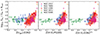 |
Fig. B.1. Comparison of metallicity measurements (i.e., 12+log(O/H)). Left: using fixed radial metallicity gradient using the O3N2 calibration (that uses the [OIII]λ5007, [NII]λ6584, Hβ and Hα lines, see Pettini & Pagel 2004). Middle: for individual HII regions using the PG16S calibration (that uses the [OIII]λ4959,5007, [NII]λ6584,6584, [SII]λ6717,6731, Hβ and Hα lines, see Pilyugin & Grebel 2016). Right: measurements from the middle panel converted to O3N2 calibration using the third panel Figure B1 in the Appendix of De Vis et al. (2019). |
Appendix C: Assuming a constant σatom in Eq. (8)
In Eq. (8) we fixed σatom to 10 km s−1. It was already highlighted in Sun et al. (2020a) that changing σatom has a minimal impact on the derived PDE estimates. In Figure C.1 we show for the PHANGS-MeerKAT galaxies that PDE derived using (i) a fixed σatom, and (ii) a varying σatom, differ only slightly.
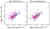 |
Fig. C.1. Our PDE estimates using a fixed σatom of 10 km s−1 (left panel) and a varying σatom (right panel). We only show the comparison for the PHANGS-MeerKAT galaxies, for which σatom derived from the line Equivalent Width (EW) maps is available (see Leroy et al. 2021b for details about EW). |
Appendix D: No galaxy-to-galaxy variation across the ΣSFR-PDE plane
In the Section 6.2 we have shown that PDE plays an important role in setting star formation. Figure D2 shows that we are unable to find significant galaxy-to-galaxy variations for ΣSFR versus PDE. We show individual measurements for individual galaxies (8 panels to the right) together with the empirical scaling relation (grey dashed lines). We note again the measurements in the PDE > 106 K cm−3 regime that showed up in Figure 12 as low ΣHI measurements which are attributed to the central regions of NGC 1566, NGC 1672, and NGC 7496, where their AGN is responsible for a H I-depression.
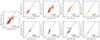 |
Fig. D.1. We show here ΣSFR against PDE for individual galaxies. We do not find any specific or significant variation between galaxy characteristic (e.g. interacting, H I dominant) |
Appendix E: Additionally detected galaxies in the PHANGS-MeerKAT field of view
We find additional galaxies that were captured within the field of view of MeerKAT. We targeted NGC 7496, but can clearly see in Figure E2 three additional galaxies. These are NGC 7496 A, NGC 7531 and ESO 291-G003. The integrated intensity map was imaged at 30″resolution. In the main part of this paper, however, we focus on galaxies that have all the relevant ancillary data available and imaged them at 15″resolution.
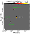 |
Fig. E.1. Additionally detected galaxies around NGC 7496. |
All Tables
Properties of our compiled dataset for NGC 1512, NGC 4535, and NGC 7496 (from PHANGS-MeerKAT; this work) and IC1954, NGC 1566, NGC 1672, NGC 3511, and NGC 5068 (from MHONGOOSE, de Blok et al. 2016).
Radii at which galaxies cross the Rmol = 1 boundary (i.e., where ΣHI ≈ ΣH2), ordered by rgal/r25.
All Figures
|
Fig. 1. Example of the extent of the emission of H I with the new MeerKAT observations. Top: three-color optical image showing star forming spiral galaxy NGC 1512 and the low-mass dwarf companion NGC 1510 in the optical (image credits: DESI Legacy Survey). The scale bar on the lower left corner indicates 20 kpc. Bottom: same as above but overlaid with H I emission contour levels of log10 0.25, 1, 1.5, 2, 2.25, 2.5, 2.75, 3 K km s−1 together with the western and southern tidal dwarf galaxies of NGC 1512 (see Section 3 for more information). |
| In the text | |
|
Fig. 2. Example of a multiwavelength view of one of our galaxies within our sample – NGC 1512. Left in red frame: MeerKAT H I observations showing on top the integrated intensity map in units of K km s−1 (moment 0), which we use in this work. Although not used in this paper, the bottom panels show the velocity field (moment 1) and the velocity dispersion (moment 2). These maps are used in Laudage et al. (2024) to analyze the neutral atomic and molecular gas kinematics in the PHANGS-MeerKAT sample. Right top in purple frame: ALMA observations of CO(2–1) from PHANGS-ALMA (Leroy et al. 2021b) showing an integrated intensity map (see Section 2.3 for CO coverage). Right bottom in blue frame: GALEX observation of FUV emission at 154 nm. The green rectangle shows the location of the interacting galaxy NGC 1510. |
| In the text | |
|
Fig. 3. Integrated intensity maps (moment 0) for H I emission (in red to yellow colors) and CO(2–1) (in purple to yellow colors) across the disks of our sample of eight nearby spiral galaxies (excluding NGC 1512, already shown in Figure 2). The corresponding beam sizes are visible in the bottom left corner of each map. The white dashed contours on the MeerKAT H I maps represent the field of view of the ALMA CO(2–1) observations, which we show next to each HI map. The CO maps cover ∼70 − 90% of the total CO emission (see Section 2.3). |
| In the text | |
|
Fig. 4. Integrated intensity maps after hexagonal sampling. The left plot shows the overall H I disk of NGC 1566. The right two panels show the enlarged versions of the green rectangle at matched field-of-view. We show here hexagonal apertures (1.5 kpc in size) on the H I and CO(2–1) maps where the circle in the lower left corner indicates the (matched) beam size (see Table 2). |
| In the text | |
|
Fig. 5. Radial extent of H I and CO in NGC 1512. This galaxy has the largest H I disk in our sample. The maximum galactocentric radius of the CO(2–1) observations is sensitive to the ALMA field-of-view (we recover ∼70 − 90% of the total CO emission, see Section 2.3). The scatter points show each individual sight line, i.e. 1.5 kpc aperture. The red-to-yellow color scale shows the point density of ΣHI and the dark-blue to yellow shows the point density of ΣH2. The white and red lines show the median within a given 1.5 kpc wide radial bin. We see that H I extends until rgal ∼ 120 kpc (that is 5 × r25 or 8 times the optical radius of the Milky Way, indicated as a purple arrow). We indicate the approximate rgal range where NGC 1510 sits with vertical dashed lines. The clumps NGC 1512-south-a, NGC 1512-south-b, and NGC 1512-west are ∼140 kpc from the center of NGC 1512. We indicate Reff, r25 and RHI as gray, pink, and orange vertical dashed lines, respectively (taken from Table 1). |
| In the text | |
|
Fig. 6. Radial extent of H I and CO in NGC 1566, NGC 1672, and NGC 3511. These galaxies have the largest H I disk extent in our sample, and exhibit special H I characteristics. We indicate Reff, r25 and RHI as grey, pink, and orange vertical dashed lines, respectively (taken from Table 1). Top: we note here two additional clumps outside of NGC 1566’s main H I disk that have been identified as additional field galaxies (see de Blok et al. 2024). Middle: toward NGC 1672 we see an increase of H I emission at rgal ∼ 70 kpc, which is the region of additional low-H I emission in the west of NGC 1672’s disk (see also Figure 3). Bottom: The hatched region from rgal = 40-120 kpc spans the low-density filamentary structure seen in the moment map (see Figure 3), which gives the impression of connecting NGC 3511 and NGC 3513. |
| In the text | |
|
Fig. 7. Radial extent of H I and CO in NGC 4535, NGC 7496, IC 1954, and NGC 3511. These galaxies have the smallest H I disk extent in our sample, and do not exhibit any peculiar H I characteristics. We show the corresponding Reff, r25 and RHI indicated as vertical dashed lines. |
| In the text | |
|
Fig. 8. Rmol against the normalized radius rgal/r25. The region below the dotted horizontal line at Rmol = 1 can be viewed as dominated by ΣHI, and the region above that line by ΣH2. Left: grey line shows a fit for all the galaxies and it crosses the Rmol = 1 boundary at rgal ∼ 0.4 r25, which means that the atomic gas on average becomes molecular inside that radius in these eight galaxies. The grey shaded region corresponds to the 3σ confidence interval. Right: colored lines show fits for individual galaxies. We list the corresponding fit parameters in Table 4. |
| In the text | |
|
Fig. 9. Rmol scaling relations. The numbered panels show linear regression fits between log10ΣH2/ΣHI against six different physical quantities that we derived in Section 4: (1) Σgas, (2) ΣSFR, (3) Σ*, (4) Z′, (5) PDE, and (6) PDE/ΣSFR. Each color represents one galaxy. The lower right panel represents the range of correlation coefficient ρ and the mean absolute ρ for all galaxies for each individual fitted quantity shown in panels (1)–(6) using a hierarchical Bayesian method (linmix, see Section 4.9). All of the properties of the presented linear regression fits are listed in Table 5. |
| In the text | |
|
Fig. 10. Rmol against PDE. Left: shown here is an enlarged version of panel 5 from Figure 9, with the fit now performed over the entire sample (purple line) with the corresponding 3σ confidence interval (purple shaded region). The black, grey, and pink lines show literature fits adopted from Sun et al. (2020a), Leroy et al. (2008), and Blitz & Rosolowsky (2006), respectively. Right: Comparison between (i) Rmol and PDE estimates from Sun et al. (2020a) for three overlapping galaxies (grey markers) and (ii) our derived Rmol and PDE (colored markers). The different shapes of the markers correspond to different galaxies. |
| In the text | |
|
Fig. 11. Illustration of different data quality used in this work compared to data used in Sun et al. (2020a). The corresponding beam sizes of ∼15″ and ∼100″ are visible in the corners. |
| In the text | |
|
Fig. 12. ΣSFR against PDE colored by ΣHI. The purple line shows our fit over the entire sample with the corresponding 3σ confidence interval. The grey dashed and dotted lines show empirical scaling relations from Kim et al. (2013) and Ostriker & Kim (2022). The black dash-dotted line shows a fit from Sun et al. (2022). We see that low ΣHI is responsible for our shallower fit compared to the literature. |
| In the text | |
|
Fig. A.1. Comparison of star formation rate surface densities using FUV+WISE4-based and the Hα-based measurements in the Rmol - ΣSFR plane. |
| In the text | |
|
Fig. B.1. Comparison of metallicity measurements (i.e., 12+log(O/H)). Left: using fixed radial metallicity gradient using the O3N2 calibration (that uses the [OIII]λ5007, [NII]λ6584, Hβ and Hα lines, see Pettini & Pagel 2004). Middle: for individual HII regions using the PG16S calibration (that uses the [OIII]λ4959,5007, [NII]λ6584,6584, [SII]λ6717,6731, Hβ and Hα lines, see Pilyugin & Grebel 2016). Right: measurements from the middle panel converted to O3N2 calibration using the third panel Figure B1 in the Appendix of De Vis et al. (2019). |
| In the text | |
|
Fig. C.1. Our PDE estimates using a fixed σatom of 10 km s−1 (left panel) and a varying σatom (right panel). We only show the comparison for the PHANGS-MeerKAT galaxies, for which σatom derived from the line Equivalent Width (EW) maps is available (see Leroy et al. 2021b for details about EW). |
| In the text | |
|
Fig. D.1. We show here ΣSFR against PDE for individual galaxies. We do not find any specific or significant variation between galaxy characteristic (e.g. interacting, H I dominant) |
| In the text | |
|
Fig. E.1. Additionally detected galaxies around NGC 7496. |
| In the text | |
Current usage metrics show cumulative count of Article Views (full-text article views including HTML views, PDF and ePub downloads, according to the available data) and Abstracts Views on Vision4Press platform.
Data correspond to usage on the plateform after 2015. The current usage metrics is available 48-96 hours after online publication and is updated daily on week days.
Initial download of the metrics may take a while.