| Issue |
A&A
Volume 688, August 2024
|
|
|---|---|---|
| Article Number | A109 | |
| Number of page(s) | 34 | |
| Section | Extragalactic astronomy | |
| DOI | https://doi.org/10.1051/0004-6361/202348297 | |
| Published online | 21 August 2024 | |
MHONGOOSE: A MeerKAT nearby galaxy H I survey
1
Netherlands Institute for Radio Astronomy (ASTRON), Oude Hoogeveensedijk 4, 7991 PD Dwingeloo, The Netherlands
e-mail: This email address is being protected from spambots. You need JavaScript enabled to view it.
2
Dept. of Astronomy, Univ. of Cape Town, Private Bag X3, Rondebosch 7701, South Africa
3
Kapteyn Astronomical Institute, University of Groningen, PO Box 800, 9700 AV Groningen, The Netherlands
4
INAF – Osservatorio Astronomico di Cagliari, Via della Scienza 5, 09047 Selargius, CA, Italy
5
Adjunct Astronomer, Green Bank Observatory, 155 Observatory Road, Green Bank, WV 24944, USA
6
Aix Marseille Univ, CNRS, CNES, LAM, Marseille, France
7
Department of Physics and Astronomy, University of Manitoba, Winnipeg, Manitoba, Canada R3T 2N2, Canada
8
INAF – Padova Astronomical Observatory, Vicolo dell’Osservatorio 5, 35122 Padova, Italy
9
International Centre for Radio Astronomy Research, The University of Western Australia, 35 Stirling Highway, Crawley, WA 6009, Australia
10
Argelander-Institut für Astronomie, Auf dem Hügel 71, 53121 Bonn, Germany
11
Instituto de Astrofísica, Departamento de Ciencias Físicas, Universidad Andrés Bello, Fernandez Concha 700, Las Condes, Santiago, Chile
12
Department of Physics and Astronomy, 102 Natural Science Building, University of Louisville, Louisville, KY 40292, USA
13
Ruhr University Bochum, Faculty of Physics and Astronomy, Astronomical Institute (AIRUB), Universitätsstrasse 150, 44801 Bochum, Germany
14
Max-Planck-Institut für Radioastronomie, Auf dem Hügel 69, 53121 Bonn, Germany
15
Department of Astronomy, The Ohio State University, 140 West 18th Avenue, Columbus, OH 43210, USA
16
Center for Cosmology and Astroparticle Physics, 191 West Woodruff Avenue, Columbus, OH 43210, USA
17
South African Astronomical Observatory (SAAO), PO Box 9, Observatory, 7935 Cape Town, South Africa
18
Southern African Larger Telescope (SALT), PO Box 9, Observatory, 7935 Cape Town, South Africa
19
Institute for Computational Cosmology, Department of Physics, Durham University, South Road, Durham DH1 3LE, UK
20
Centre for Extragalactic Astronomy, Department of Physics, Durham University, South Road, Durham DH1 3LE, UK
21
Max Planck Institute for Astronomy, Königstuhl 17, 69117 Heidelberg, Germany
22
Instituto de Astrofísica de Andalucía-CSIC, Glorieta de la Astronomía s/n, 18008 Granada, Spain
23
CSIRO, Space & Astronomy, PO Box 1130, Bentley, WA 6102, Australia
24
Laboratoire de Physique et de Chimie de l’Environnement, Observatoire d’Astrophysique de l’Université Ouaga I Pr Joseph KiZerbo (ODAUO), 03 BP 7021, Ouaga 03, Burkina Faso
25
Observatoire de Paris, Collège de France, Université PSL, Sorbonne Université, CNRS, LERMA, Paris, France
26
Centre for Astrophysics Research, University of Hertfordshire, College Lane, Hatfield AL10 9AB, UK
27
E.A. Milne Centre for Astrophysics, University of Hull, Hull HU6 7RX, UK
28
Department of Physics and Electronics, Rhodes University, PO Box 94, Makhanda 6140, South Africa
29
Australia Telescope National Facility, CSIRO Astronomy and Space Science, PO Box 76, Epping, NSW 1710, Australia
30
Western Sydney University, Locked Bag 1797, Penrith South, NSW 1797, Australia
31
Department of Astronomy, Case Western Reserve University, 10900 Euclid Avenue, Cleveland, OH 44106, USA
32
Department of Physics and Space Science, Royal Military College of Canada, PO Box 17000, Station Forces Kingston, ON K7K 7B4, Canada
33
Department of Physics, Engineering Physics and Astronomy, Queen’s University, Kingston, ON K7L 3N6, Canada
34
Max Planck Institute for Extraterrestrial Physics, Gießenbachstraße 1, 85748 Garching, Germany
35
University of Wisconsin-Madison, Department of Astronomy, 475 N. Charter Street, Madison, WI 53706-1582, USA
36
Jodrell Bank Centre for Astrophysics, School of Physics and Astronomy, University of Manchester, Oxford Road, Manchester M13 9PL, UK
37
Department of Physics and Astronomy, University of the Western Cape, Robert Sobukwe Rd, Bellville 7535, South Africa
38
The Inter-University Institute for Data Intensive Astronomy (IDIA), University of Cape Town, Private Bag X3, Rondebosch 7701, South Africa
39
National Radio Astronomy Observatory, PO Box O, Socorro, NM 87801, USA
40
Department of Physics and Astronomy, MSC07 4220, 1 University of New Mexico, Albuquerque, NM 87131, USA
41
Centre for Space Research, North-West University, Potchefstroom 2520, South Africa
42
Department of Physics, Virginia Polytechnic Institute and State University, 50 West Campus Drive, Blacksburg, VA 24061, USA
43
Wits Centre for Astrophysics, School of Physics, University of the Witwatersrand, 1 Jan Smuts Avenue, Johannesburg 2000, South Africa
44
Department of Physics and Astronomy, Sejong University, Seoul 05006, South-Korea
45
NASA Headquarters, 300 Hidden Figures Way, SE, Mary W. Jackson NASA HQ Building, Washington, DC 20546, USA
46
School of Physics and Astronomy, Cardiff University, Queens Building, The Parade, Cardiff CF24 3AA, UK
47
Department of Physics and Astronomy, Rutgers, The State University of New Jersey, 136 Frelinghuysen Road, Piscataway, NJ 08854-8019, USA
48
Department of Physics and Astronomy, The University of Manchester, Manchester M13 9PL, UK
49
School of Mathematical and Physical Sciences, Macquarie University, Balaclava Road, North Ryde, Sydney, NSW 2109, Australia
Received:
17
October
2023
Accepted:
27
March
2024
Abstract
The MHONGOOSE (MeerKAT H I Observations of Nearby Galactic Objects: Observing Southern Emitters) survey maps the distribution and kinematics of the neutral atomic hydrogen (H I) gas in and around 30 nearby star-forming spiral and dwarf galaxies to extremely low H I column densities. The H I column density sensitivity (3σ over 16 km s−1) ranges from ∼5 × 1017 cm−2 at 90″ resolution to ∼4 × 1019 cm−2 at the highest resolution of 7″. The H I mass sensitivity (3σ over 50 km s−1) is ∼5.5 × 10⁵ M⊙ at a distance of 10 Mpc (the median distance of the sample galaxies). The velocity resolution of the data is 1.4 km s−1. One of the main science goals of the survey is the detection of cold accreting gas in the outskirts of the sample galaxies. The sample was selected to cover a range in H I masses from 107 M⊙ to almost 1011 M⊙ in order to optimally sample possible accretion scenarios and environments. The distance to the sample galaxies ranges from 3 to 23 Mpc. In this paper, we present the sample selection, survey design, and observation and reduction procedures. We compared the integrated H I fluxes based on the MeerKAT data with those derived from single-dish measurement and find good agreement, indicating that our MeerKAT observations are recovering all flux. We present H I moment maps of the entire sample based on the first ten percent of the survey data, and find that a comparison of the zeroth- and second-moment values shows a clear separation in the physical properties of the H I between areas with star formation and areas without related to the formation of a cold neutral medium. Finally, we give an overview of the H I-detected companion and satellite galaxies in the 30 fields, five of which have not previously been cataloged. We find a clear relation between the number of companion galaxies and the mass of the main target galaxy.
Key words: galaxies: dwarf / galaxies: evolution / galaxies: ISM / galaxies: spiral / radio lines: galaxies
© The Authors 2024
 Open Access article, published by EDP Sciences, under the terms of the Creative Commons Attribution License (https://creativecommons.org/licenses/by/4.0), which permits unrestricted use, distribution, and reproduction in any medium, provided the original work is properly cited.
This article is published in open access under the Subscribe to Open model. This email address is being protected from spambots. You need JavaScript enabled to view it. to support open access publication.
1. Introduction
The evolution of the baryonic matter in the Universe can to a large degree be described as the gradual transformation of primordial atomic hydrogen into galaxies over cosmic time. This transformation involves physical processes on many scales, from the size of galaxy clusters to those of individual gas clouds within a galaxy. These processes, such as gas infall, collapse of clouds, formation of stars, feedback due to stellar winds, and supernovae, form part of the baryon cycle. Although many of them act on subgalactic scales, they nevertheless affect the evolution of galaxies as a whole.
The only place where a comprehensive detailed survey of these processes can be made is the nearby Universe: locally we can study all aspects of the baryon cycle in detail. Resolved observations of the cold gas, and, specifically of neutral hydrogen (H I) can contribute to determining how galaxies acquire their gas, how star formation is sustained, and ultimately how the dark and visible matter interact to determine and regulate the evolution of galaxies.
We concentrate here on the first issue, that is, the origin of the gas in galaxies. This question first arose from the observation that in the inner regions of nearby spiral galaxies, timescales for the consumption of gas by star formation are much shorter than a Hubble time, even though the star formation rate (SFR) has been approximately constant over most of the lifetime of the galaxies (e.g., Kennicutt 1998; Bigiel et al. 2011; Leroy et al. 2013; Fraternali & Tomassetti 2012). If galaxies are to continue forming stars at their current rate beyond the current epoch, there must be a gas supply external to galaxies. A similar argument can also be made based on observations of high-redshift galaxies (e.g., Saintonge et al. 2013; Tacconi et al. 2018). These form stars at a much higher rate than that observed in the local Universe. This would imply a strong decrease in the gas content of galaxies between then and now; yet we observe an almost constant density, again implying there is an external supply of gas (see, e.g., Walter et al. 2020). In other words, we observe that the gas depletion time for high-redshift galaxies is ∼1 Gyr or less (Saintonge et al. 2013; Tacconi et al. 2018) and yet most galaxies are not quenched and keep forming stars for a much longer time until today.
Galactic disks can, in principle, be replenished by accreting gas-rich companion galaxies, but the slope of the H I mass function is not steep enough for small companions to supply larger galaxies with a substantial amount of gas for a sufficiently long time (Sancisi et al. 2008). In addition, observations suggest that gas-rich mergers can, at most, provide 20% of the gas required to maintain the SFR in nearby late-type galaxies (Di Teodoro & Fraternali 2014). This implies that spirals have to accrete directly from the intergalactic medium (IGM).
The presence of cold gas in the halos of our Milky Way and other galaxies has been known for several decades (see, e.g., Wakker & Woerden 1997; Oosterloo et al. 2007; Sancisi et al. 2008; Heald et al. 2011 and the reviews by Putman et al. 2012 and Tumlinson et al. 2017). The H I in some halos may be part of a star-formation-driven “galactic fountain” (Shapiro & Field 1976). This galactic fountain has been proposed to lead to an “indirect” cold-gas-accretion mechanism, where the gas that is expelled from the disk, drags additional halo gas along as it returns to the disk (Marasco et al. 2012; Fraternali 2017; Marasco et al. 2019).
This is suggested, for example, for the galaxy NGC 2403 by the observation that most of its extraplanar H I has a similar projected radial distribution to the star formation in the disk and that it has disk-like kinematics: rotating but lagging behind the main disk (see, e.g., Fraternali et al. 2001). Similar conclusions were reached for nearby galaxy NGC 253 (Lucero et al. 2015). However, we note that in NGC 2403, we also observe H I in the halo that likely has an external origin (Veronese et al. 2023), and indeed some of the H I complexes found outside of the main H I disks of galaxies are counter-rotating with respect to the disk, confirming that they cannot have originated from it. Numerical simulations (e.g., Kere et al. 2005; Ramesh et al. 2023) predict that filaments of cooler gas from the IGM can penetrate the hot halos surrounding galaxies and deposit gas onto the disk. This process is called cold accretion. These filaments are a prediction of high-resolution cosmological hydrodynamical simulations of structure formation (e.g., Davé et al. 1999; Crain et al. 2016; Ramesh et al. 2023), which suggest that most of the baryons at low redshift are in a warm-hot (T ∼ 105 − 107 K) intergalactic medium and most of the gas in the cosmic web is therefore ionized and difficult to observe directly. To detect the smaller fraction of cooler (T < 104 K) baryons in the cosmic web, an H I column density sensitivity of ∼1017 − 18 cm−2 is required (Popping et al. 2009).
It is in the context of this cold accretion that the study of H I halos of galaxies is relevant: it could provide direct observations of the accretion of gas onto galaxies as well as a strong observational test for models of galaxy evolution. An extensive study of the H I halos of nearby spiral galaxies was made by the Hydrogen Accretion in LOcal GAlaxieS (HALOGAS) project on the Westerbork Synthesis Radio Telescope (WSRT; Heald et al. 2011). To this end, 22 disk galaxies were mapped down to an H I column density limit of ∼1019 cm−2, which is an order of magnitude lower than the surface densities typically found in star-forming H I disks. The results of HALOGAS indicate that some galaxies have more extended low-column-density emission, while others do not: extended H I distributions have been detected in about 12 of the 22 galaxies observed. It is possible that some of this gas is related to star formation and galactic fountain processes (Marasco et al. 2019), but external accretion cannot be excluded. The average rate at which cold neutral hydrogen gas is accreted by the HALOGAS galaxies is between 0.05 and 0.09 M⊙ yr−1 (Kamphuis et al. 2022), with the exact value depending on the treatment of the amount of H I detected by the Green Bank Telescope (GBT) but not by the WSRT. This accretion rate is generally lower than the SFR (cf. Table 4 in Kamphuis et al. 2022). If in the HALOGAS sample, the H I accretion rate balances the star formation rate, direct accretion must occur at much lower neutral gas column densities than detected by HALOGAS and on spatial scales not resolved by the GBT.
Very deep single-dish H I observations show the presence of H I at these very low-column densities. Braun & Thilker (2004), for example, observed low-column-density features around and between M31 and M33 and, using the WSRT as a single dish, reached a 3σ limit over 16 km s−1 of 1.1 × 1017 cm−2, but with an angular resolution of ∼49′. Further deep observations with the GBT of the HALOGAS (Heald et al. 2011) and The H I Nearby Galaxy Survey (THINGS; Walter et al. 2008) galaxies are described in Pisano (2014), de Blok et al. (2014), and Pingel et al. (2018). These reach a 3σ over 16 km s−1 sensitivity of ∼6 × 1017 cm−2 at an angular resolution of about 9′ or ∼14 kpc and ∼24 kpc at the median distances of the THINGS and HALOGAS galaxies, respectively. However, sheer column density sensitivity is not enough, as these relatively coarse spatial resolutions already suggest. Wolfe et al. (2013, 2016) show that the diffuse ∼1017 cm−2 low-column-density gas between M31 and M33 observed by Braun & Thilker (2004) is resolved in several kiloparsec-sized clouds with peak column densities of a few times 1018 cm−2 when observed at higher spatial resolutions.
To properly detect and characterize accretion features both a kpc-scale (or better) spatial resolution and a column density sensitivity of ∼1018 cm−2 (or better) are thus needed. Surveys such as THINGS (Walter et al. 2008) and HALOGAS (Heald et al. 2011) have concentrated on either obtaining a high spatial resolution or a high column-density sensitivity. Optimising both simultaneously is rarely an option; this has so far limited our knowledge of how any low-column-density gas is connected with the cosmic web and where accretion occurs.
2. The MHONGOOSE survey
The MeerKAT radio telescope (Jonas 2018; Camilo 2018; Mauch et al. 2020) is making it possible to take this large step forward. MeerKAT consists of 64 dishes each with an effective diameter of 13.5m, located in the Karoo semi-desert in South Africa. The array has a compact and dense core (the shortest baseline being 29m), with 70% of the collecting area located close to the centre of the array, and with longest core baselines of 1 km. The rest of the array is distributed at larger distances, to a maximum baseline of 7.7 km. This combination of a dense core and long baselines means the telescope has the ability to produce high-resolution imaging, while retaining a good column density sensitivity. A third factor contributing to the high sensitivity is the low system temperature of the receivers. At 1.4 GHz, the effective system temperature is Tsys/η ≃ 20.5 K (where η is the antenna efficiency).
The array design of MeerKAT is such that the noise level for observations producing beam sizes between ∼6″ and ∼90″ is approximately flat (see Fig. 1). MeerKAT is therefore not optimized for one particular resolution, but allows high-quality imaging over a large range in resolutions using weighting or tapering.
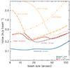 |
Fig. 1. Noise level as a function of resolution for the HALOGAS, THINGS, and MHONGOOSE surveys. The blue curve shows that the MHONGOOSE survey has a flat noise distribution, meaning equally sensitive imaging can be obtained over a large range of resolutions between ∼6″ and ∼90″. The dashed brown curve shows the HALOGAS survey, with an optimal sensitivity at around ∼20″. The dashed red curve represents the THINGS survey. This is a combination of three separate VLA array configurations (also shown at the top of the plot calculated using the correct relative observing times). THINGS has optimal sensitivity at around ∼15″ and ∼50″. All noise values are calculated over a 5 km s−1 channel. |
Thanks to the combination of exquisite column density sensitivity, high spatial resolution (down to ∼7″ for H I) and a large field of view with a primary beam full width at half-maximum (FWHM) diameter of 1°, we can study nearby galaxies in H I at the required quality to characterize any low-column density H I that may be accreting onto a galaxy.
MHONGOOSE (MeerKAT H I Observations of Nearby Galactic Objects: Observing Southern Emitters) is a MeerKAT Large Survey Project designed to produce ultra-deep H I observations of 30 nearby gas-rich spiral and dwarf galaxies in order to detect and characterize any low-column density, potentially infalling, atomic gas, and to probe its link to star formation (see also de Blok et al. 2016, 2020). These deep observations can provide information on gas flows into and out of the galaxy disks, accretion from the IGM, the fuelling of star formation, the connection with the cosmic web and even the possible existence of low-mass cold dark matter (CDM) halos. The relation between dark and baryonic matter and the distribution of dark matter within galaxies can also be comprehensively studied due to the high resolution combined with high sensitivity. The large field of view of MeerKAT means a significant fraction of the virial volumes of the target galaxies can be observed.
For the MHONGOOSE survey, each sample galaxy is observed for 55 hours in order to reach a 3σ over 16 km s−1 sensitivity limit of 5 × 1017 cm−2 to detect the low-column density component discussed above. Such column densities are close to three orders of magnitude below those typically found in the star-forming disks of galaxies and equal those of the accreting cool neutral gas as predicted by many numerical simulations (Kere et al., 2005; Popping et al. 2009; Ramesh et al. 2023).
Figure 2 compares the MHONGOOSE column density sensitivities with those from previous H I surveys using both interferometers and single-dish telescopes. Interferometric targeted surveys shown here are THINGS (Walter et al. 2008), HALOGAS (Heald et al. 2011), the Westerbork H I Survey Project (WHISP; van der Hulst et al. 2001), the Local Irregulars That Trace Luminosity Extremes, The HI Nearby Galaxy Survey (LITTLE THINGS; Hunter et al. 2012) and the Local Volume H I Survey (LVHIS; Koribalski et al. 2018). Also shown is the untargeted Widefield ASKAP L-band Legacy All-sky Blind surveY (WALLABY; Koribalski et al. 2020). For the single-dish observations we show the column density sensitivities for the H I Parkes All Sky Survey (HIPASS; Barnes et al. 2001; Meyer et al. 2004), the Arecibo Legacy Fast ALFA (ALFALFA; Haynes et al. 2018), the Arecibo Galaxy Environment Survey (AGES; Auld et al. 2006), deep observations of M31 (Wolfe et al. 2016) and NGC 2903 (Irwin et al. 2009), as well as a number of deep GBT and Parkes observations of nearby galaxies (Sorgho et al. 2018, Sardone et al. 2021, Pingel et al. 2018, D.J. Pisano, priv. comm.). We also show a number of representative deep H I observations taken with the Five-hundred-meter Aperture Spherical Telescope (FAST) from Xu et al. (2022) and Liu et al. (2023).
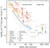 |
Fig. 2. Sensitivity versus resolution in H I surveys. Colored symbols show the 3σ column density sensitivity over 16 km s−1 for various interferometric and single-dish surveys, as indicated by the labels and legend and listed in the text. The thick blue line shows the observed MHONGOOSE sensitivities. MHONGOOSE reaches single-dish sensitivities but at a 10–50 times better angular resolution. To give an indication of the physical scales: at 10.3 Mpc (the median distance of the MHONGOOSE sample), 10″ corresponds to 0.5 kpc. Galaxies that are part of a sample with a fixed angular resolution (THINGS 30″, GBT, and PKS) were given small, random horizontal offsets for clarity. References are given in the text. |
To ensure a proper comparison we have taken the noise per channel and the channel widths from the source papers or the corresponding publicly available data and homogenized these quantities to a common channel width of 16 km s−1, assuming square-root scaling of noise with channel-width. A 16 km s−1 channel width corresponds approximately to the FWHM of an H I line with a velocity dispersion of 7 km s−1, which is comparable to the lowest values seen in previous H I observations of nearby galaxies (Ianjamasimanana et al. 2017).
In Fig. 2 we show the sensitivities of these H I surveys and compare these with the observed sensitivity of MHONGOOSE. It is clear that at all resolutions the MHONGOOSE data are significantly more sensitive than previous interferometric observations. Note that the sensitivity does not change simply as the inverse of the beam size squared (which would be a straight line with a slope of −2) as one might expect. This is due to the different weightings and taperings used to produce the data at the various resolutions. We return to this in Sect. 5.6.
For comparison, we also show estimated sensitivities for H I surveys on SKA-MID. These are simply calculated by scaling up the MeerKAT collecting area to the SKA-MID “baseline design” collecting area (i.e., the equivalent of 64 MeerKAT dishes with 13.5m diameter and 133 SKA dishes with 15m diameter) and should therefore only be regarded as indicative, as they do not take into account potentially different baseline distributions, dish designs, or system temperatures.
A striking aspect of the comparison is that between ∼30″ and ∼100″, MHONGOOSE is probing unexplored territory, with observations that have the column density sensitivity of deep single-dish H I observations of the Local Universe, but at an angular resolution that is more than an order of magnitude better. With these observations it will therefore be possible to investigate the low-column density H I, from the outskirts of the star-forming disks out into the far reaches of the dark matter halo.
3. Sample selection
One of the main goals of MHONGOOSE is to trace accretion and star formation processes over a large range in galaxy properties. It is thus important to ensure that within the limited observing time available a representative range of H I masses, stellar masses, star formation rates and rotation velocities (and hence, halo masses) is sampled. Furthermore, to isolate accretion features from tidal and interaction features as much as possible, strongly interacting galaxies and dense environments are to be avoided.
Primary criteria for the sample selection are that the galaxies should have been detected in H I and located in the southern hemisphere. This makes the HIPASS catalog (Meyer et al. 2004) a natural starting point. To ensure the availability of a significant set of multi-wavelength data, we limited our selection to HIPASS galaxies that are part of the Survey of Ionization in Neutral Gas Galaxies (SINGG; Meurer et al. 2006) and the Survey of Ultraviolet emission in Nearby Galaxies (SUNGG; Wong et al. 2016). These surveys collected Hα, optical, infrared and ultraviolet data for a large number of HIPASS-detected nearby galaxies.
The SINGG/SUNGG criteria were as follows:
-
(i)
HIPASS peak flux density > 50 mJy (3.8σ in HIPASS),
-
(ii)
Galactic latitude |b|> 30°,
-
(iii)
Projected distance from the center of the Large (Small) Magellanic Cloud > 10° (> 5°),
-
(iv)
Galactic standard of rest velocity > 200 km s−1.
This SINGG/SUNGG protosample was divided in bins of 0.2 dex in log(MH I) and in each bin the closest 30–40 galaxies were selected. This gave a flat number distribution in the range 8.5 < log(MH I/M⊙)< 10.5, with an additional, small number of galaxies around log(MH I/M⊙)∼7.0 and log(MH I/M⊙)∼11. Most of these selected galaxies have a radial velocity < 2000 km s−1 with a median velocity of 1300 km s−1. These criteria resulted in the final SINGG sample of 468 galaxies as published in Meurer et al. (2006). The key characteristic of this selection is that it was done uniformly in log(MH I) in order to guarantee the broadest possible range in H I masses.
For MHONGOOSE we further narrowed down the SINGG sample by requiring that for a given galaxy, a complete set of Hα, R-band and GALEX ultra-violet data was available. This reduced the number of galaxies to 151. To retain sufficient spatial resolution, we furthermore removed all galaxies with a distance D > 30 Mpc (heliocentric velocity vhel > 2100 km s−1). In addition, we only selected galaxies with a southern declination, and we excluded the survey area of the MeerKAT Fornax Survey (Serra et al. 2023). We additionally checked that the potential sample galaxies were not located in the densest environments (i.e., inner parts of galaxy clusters or major galaxy groups). Galaxies that were located in the outer parts of (smaller) groups were retained (as were, obviously, isolated galaxies). This enables quantifying the effects of environment on accretion processes in medium- to low-density environments, without the target galaxies themselves being majorly affected by the environment. Studies of isolated galaxies have shown that the gas captured from companion galaxies and galactic fountain processes (due to SF and Active Galactic Nuclei [AGN]) are minimized there (Jones et al. 2017; Espada et al. 2011a, 2011b; Leon et al. 2008; Sabater et al. 2012; Lisenfeld et al. 2007). These criteria resulted in a sample of 88 galaxies.
As the goal of MHONGOOSE is to characterize the low-column density H I over a large range in H I masses, we aimed for a flat number distribution in log(MH I) over the available mass range 6.0 < log (MH I/M⊙) < 10.5, analogous to SINGG. To compensate for the smaller number of galaxies, we used six bins each with a width of 0.5 dex, except for the lowest-mass bin, which we defined as log(MH I/M⊙)< 8.0.
The final sample size of 30 galaxies was set by the assigned observing time and the desired column density sentivity. This total number implies a total of five galaxies per mass bin. To optimize the selection for the science objectives of the survey, we required that galaxies be in one of three well-defined inclination categories as follows: i) (close to) face-on, ii) (close to) edge-on and iii) inclination (close to) 60 degrees. Face-on allows the best characterization of the morphology of the interstellar medium (ISM), as well as determination of vertical motions. Edge-on allows an unambiguous characterization of the vertical structure of the ISM and possibly the dark matter distribution out of the disk plane. The intermediate inclination range allows (following a limited amount of modeling) determination of both, and can be used to tie results from edge-on and face-on classes together. It is also an optimal inclination for rotation curve measurements and mass-modeling of the galaxy.
Selection of the final 30 galaxies was done in two steps. In the first step, optical SINGG and Digital Sky Survey images were examined and galaxies that were affected by bright foreground stars were rejected. In addition, we rejected cases where the galaxy was too big to comfortably fit in the 1° FWHM MeerKAT primary beam. This to avoid reduced sensitivity to H I in the outer parts of the galaxies (due to the primary beam attenuation) and to ensure mosaicking was not needed. Generally we insisted that the optical diameter was smaller than 15′ (though few galaxies actually reached that size). In SINGG, the optical diameter is determined from optical surface brightness profiles and corresponds to twice the radius beyond which no detectable R-band, Hα, or UV emission is found. Meurer et al. (2013) show that this radius appears to correspond to the edge of the stellar disk.
We also did not include galaxies that were clearly strongly interacting. Finally, we checked that no extremely bright radio continuum sources were present within or close to the galaxy positions. All of this resulted in the rejection of 11 galaxies.
We then stepped through each of the mass bins and used the SINGG imaging to select in each bin the most optimal edge-on, face-on, and intermediate-inclination galaxies. Factors that went into this were how close the galaxies were to the preferred inclinations (as judged from the apparent major to minor axis ratios estimated from the SINGG R-band images), their angular sizes, and their distances (where the nearest galaxies were preferred). A secondary condition was to ensure that a range in star formation rates (as judged from the SINGG Hα SFR measurements) was covered for each bin.
This resulted in the final sample of 30 galaxies. These are listed in Table 1 along with some fundamental properties. We note that some properties listed here are different from those given in the earlier sample table in de Blok et al. (2020). That table lists the sample with the galaxy parameters originally used for the sample selection as based on parameters and distances from SINGG/SUNGG. In the current paper, we have adopted more recent distance estimates for the galaxies (including Tip of the Red Giant Branch [TRGB] measurements). These revised distances resulted in small changes in distance-dependent properties (such as the H I mass), sometimes resulting in a galaxy moving to a different H I mass bin. These changes have no significant impact on the final science goals. The sample still covers the desired large range in H I mass as well as a representative range in (gas-rich) galaxy properties. The current Table lists the galaxies in order of H I mass assuming the revised distances. For the median distance of the galaxies in the MHONGOOSE sample (10.3 Mpc), 10″ corresponds to 0.5 kpc. H I-related parameters listed in the Table are based on the observations presented in this paper. The inclination values are based on the optical axis ratios and should be regarded as indicative only.
Properties of galaxies in the MHONGOOSE sample.
In Table 1 we also give the stellar masses and star formation rates based on WISE infrared measurements. The stellar masses were derived using the new GAMA Stellar Masses calibration and (light and colors) method of Jarrett et al. (2023). The star formation rates are a combination mid-IR and UV SFR based on the method described in Cluver et al. (in prep.). Figure 3 shows the distribution of the MHONGOOSE galaxies along the SFR-M⋆ main sequence (defined by the upper ridges in the diagrams). As the sample was selected to be representative of gas-rich, star-forming galaxies, it therefore covers the main sequence well. The only galaxy not on it is NGC 1371 (J0335–24), which has a low SFR for its stellar mass.
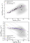 |
Fig. 3. Star formation rates of the MHONGOOSE galaxies plotted against their stellar masses. Top panel: the SFR as derived using the method described in Cluver et al. (in prep.) based on mid-IR and UV SFRs. The stellar masses are derived from WISE W3 and W4 luminosities as described in Jarrett et al. (2023). Background grayscale and gray contours show the distribution of galaxies in the local Universe based on mid-IR and UV data (Jarrett & Cluver, in prep.). The MHONGOOSE sample was selected to be representative of the SFR–M⋆ main sequence (the upper ridge of the distributions) and almost all galaxies are indeed on this sequence. Only NGC 1371 (J0335–24) has a low SFR for its mass. Galaxies with uncertain SFR values are not plotted (see Table 1). UGCA320 (J1303–17b) has a low S/N in the WISE observations as indicated by the diamond symbol. The purple dashed curve shows the average trend derived in Cluver et al. (in prep.). Bottom panel: this shows the specific SFR of the MHONGOOSE galaxies plotted against stellar mass. Symbols and curves as in top panel. In addition, the blue curve shows a fit to the data presented in Leroy et al. (2019). The diagonal gray dashed lines indicate corresponding SFR values in M⊙ yr−1. |
The MHONGOOSE sample galaxies span a range of galaxy environments, although, as described above, the selection was intentionally biased against those galaxies residing in the densest environments. Using the group catalog from Kourkchi & Tully (2017), we quantify the group environment for all 30 galaxies. Of our sample galaxies, 13 are “isolated”; that is, not in a group with another galaxy although they are still in larger associations. The remaining 17 galaxies reside in groups with anywhere from 2–31 members. Their dynamical group masses range from those of dwarf galaxy associations (≲1012 M⊙) or single, massive galaxies up to – for a few galaxies – those of small groups (∼1013 M⊙).
The identification and masses of all groups and associations as listed in the Kourkchi & Tully (2017) catalog are given in Table 2. A number of galaxies are found to be part of the same groups or associations as indicated in Table 2.
Group membership and halo properties of the galaxies in the MHONGOOSE sample
In addition, we use the stellar masses and distances given in Table 1 to calculate the halo mass M200 using the stellar mass-halo mass relation given in Moster et al. (2013). Using standard cosmology (H0 = 69 km s−1 Mpc−1, ΩΛ = 0.27) we also derive the virial radius R200 for the target galaxies. We also list the ratio of a 1.5° field of view (cf. Sect. 5.7) in kpc at the distance of the galaxy, and the virial diameter D200 = 2R200. Note that we have made no attempt to homogenize the Kourkchi & Tully (2017) and Moster et al. (2013) numbers, so some differences may exist in halo or group masses due to different methods, assumptions or input data.
4. Observations
The MeerKAT MHONGOOSE observations started in October 2020. For ease of scheduling, the 55h of observing time per galaxy are divided into 10 observations of 5.5h. These consist of five “rising” observations and five “setting” ones, each of which is referred to as a “single track” in this paper. The complete 55h observation is referred to as the “full-depth” data.
The rising observations generally start sometime in the first 1.5 h after the source has become visible to MeerKAT, and end when the source is close to transit. The setting observations start close to transit and generally end in the last 1.5 h before it crosses MeerKAT’s observing horizon. There is some overlap between rising and setting tracks close to transit. The amount of overlap depends on the declination of the galaxy but is never more than 1.5 h.
A typical 5.5h observation consists of 10 mins of observing time on one of the primary calibrators J1939–6342 or J0408–6545. This is then followed by five cycles of (i) two mins on a secondary or phase calibrator and (ii) a subsequent ∼55 min on the target galaxy. The duration of the latter varies slightly from galaxy to galaxy to take into account the different slewing times while staying within the 5.5h overall duration.
If J1939–6342 was used as the primary calibrator, two additional three-minute observations of a polarisation calibrator were inserted between different cycles. If J0408–6545 was used, a polarization calibrator was observed for three minutes at the end of every phase calibrator-target cycle. This increased number of polarization calibrator observations reflects the less well-characterized polarisation properties of J0408–6545. However, since we are only concerned with the Stokes I data, we do not discuss the polarization aspects here.
A small number of observations deviated from our standard observing template. For J0008–34, J0031–22 and J2257–41 no suitable polarization calibrator was available during the rising observations, so these were extended to 6.5h. The corresponding setting observations were reduced to 4.5h.
We used the c856M4k_n107M SKARAB correlator mode, allowing for a 32k narrow band (primarily used for H I studies) and a 4k wide band (primarily used for continuum and polarization studies) to be used simultaneously. The narrow band has 32 768 channels of 3.265 kHz (0.7 km s−1 at the H I rest-frequency) each, giving a total bandwidth of 107 MHz. The 4k-mode gives 4096 channels of 208.984 kHz (∼43 km s−1 at the H I rest-frequency), covering the total bandwidth of MeerKAT of 856 MHz. For the MHONGOOSE observations, the central topocentric frequency of the 32k narrow-band was always set to 1390 MHz. For the 4k-mode this value was 1284 MHz. Both modes observed four polarizations, though for the narrowband mode (H I) we only used the HH and VV polarisations. The correlator data were integrated over 8s in the correlator before being output.
To ensure high-quality data, observations were only started if there were 58 or more active antennas present in the array. As the science critically depends on the detection of diffuse low-column density gas, additional checks were made prior to observing to ensure that a sufficient number of short baselines was present in the array, with the strictest checks for the shortest baselines. An overview of the required fraction of the number of total baselines as a function of baseline length is given in Table 3.
Baseline requirements.
A small number of early observations were done partly during daytime, but it was quickly found that solar radio frequency interference (RFI) had a severe impact on the shortest baselines. Observations that were too severely affected were redone, while for less-affected ones, baselines shorter than 1.5 kλ (or 315m for rest-frame 21-cm emission) were flagged. To avoid solar RFI affecting the short baselines, all other observations were done at night time.
5. Data reduction
After an observation was completed and deposited in the SARAO MeerKAT archive, we extracted the data covering the channel range 16 384–26 383 (10 000 channels) from the 32k narrowband data set retaining only the HH and VV polarisations. This covers the topocentric frequency range 1390.0–1422.7 MHz. These data were binned by two channels leading to a 5000-channel measurement set with a channel width of 6.53 kHz (1.4 km s−1). The data were then processed using the CARACal data reduction pipeline1 (Józsa et al. 2020). As the observations cover multiple years, and MHONGOOSE observations took place simultaneously with CARACal development, several (pre)releases of CARACal were used. Where necessary data were rereduced to ensure consistent outcomes.
CARACal is a Python-based, containerized pipeline that uses a “best-of” approach to link together reduction and analysis tasks and applications from various radio astronomy packages to optimally reduce the data, passing it seamlessly between the various reduction stages using Stimela (Makhathini 2018). These stages consist of:
-
(i)
Flagging the calibrators;
-
(ii)
Deriving and applying the cross-calibration to the target;
-
(iii)
Flagging the target;
-
(iv)
Imaging the continuum for several cycles of self-calibration;
-
(v)
Transferring the self-calibration solutions to the original measurement set;
-
(vi)
Using the self-calibration sky model to subtract the continuum from the original measurement set;
-
(vii)
Creating and deconvolving the spectral line H I data cubes.
We describe these steps in more detail below. Much of the reduction procedure was developed in collaboration with the MeerKAT Fornax Survey (Serra et al. 2023). The description given here should therefore be regarded as complementary to that given in Serra et al. (2023). Unless stated otherwise, all software tasks mentioned below in Sects. 5.1–5.7 were executed as part of the CARACal pipeline environment. All reduction was done on the dedicated MeerGas cluster at ASTRON consisting of four computing nodes with 128 cores and 1 Tb of memory each.
5.1. Cross calibration
The calibrator observations were split off in a separate measurement set and flagged for shadowing and RFI where necessary. For the latter aoflagger (as included in CARACal) searched and flagged in Stokes Q. The frequency range 1419.8–1421.3 MHz (+125 to −190 km s−1) was also flagged to avoid contamination from Galactic emission.
For each observation the primary calibrator was used to derive the delay, gain and bandpass calibration using baselines longer than 150m. To improve the signal-to-noise ratio (S/N), the bandpass was smoothed using a 9-channel box-car filter. Any gaps in the bandpass (e.g., due to the flagging of the Galactic emission) were interpolated. A second cycle of flagging and calibrating then refined these solutions, which were subsequently applied to the secondary calibrator. The latter was used to track the gain and phase variations over time. These time-dependent solutions were also derived twice with an intermediate flagging step. The final solutions were then applied to the target observations.
5.2. Self calibration and continuum subtraction
The cross-calibrated target scans were checked for shadowing (where the line-of-sight to the source is partially or fully blocked by another antenna) and RFI and, when found, flagged. The clean RFI environment at MeerKAT, and the targets being located in the protected frequency band, meant that on average only 1–2 percent of the data were flagged.
For the self-calibration procedure the target measurement set was binned in frequency to a channel width of 1 MHz. The frequency range covering Galactic emission was flagged, as well as the frequency range of the target galaxy. The latter was done to prevent bright H I features (present for some galaxies) from entering the self-calibration procedure.
Three cycles of imaging and self-calibration were then performed using three spectral solution intervals of ∼10 MHz each. During each cycle, the data were deconvolved and imaged (using wsclean; Offringa et al. 2014) to progressively deeper limits from 5 times the noise for the first imaging run, to 3.5 times the noise for final imaging. We imaged an area of 3 × 3 degrees, using a robust weighting value of −0.5, a taper of 10″ and a pixel size of 4″. The SoFiA source finder (Serra et al. 2015) (as implemented in CARACal) was used to automatically create a mask of the sky based on the output cleaned image. Care was taken that a sufficiently large window for the noise measurement was chosen such that bright, extended continuum emission from some of the target galaxies did not affect the measured noise levels and therefore the self-calibration procedure. Using this mask, a new image and sky model were created. This sky model was used for the self-calibration, after which a new cycle of image, mask and sky-model calibration was started, followed by further self-calibration. All cycles were phase-calibration only. In this way the three cleaning and self-calibration cycles to progressively larger depths lead to the final solutions.
The self-calibration solutions were interpolated in frequency and transferred to the cross-calibrated target measurement set. The most recent self-calibration sky-model clean components were also transferred to the target measurement set at this stage, and subsequently subtracted using the Crystalball software in CARACal. This step is time-consuming and accounts for one-third to one-half of the total processing time.
A second follow-up continuum subtraction using the CASA task mstransform within CARACal was used to subtract any residual continuum by fitting a first or second-order polynomial to the line-free visibilities. A catalog of known H I sources was used to define the line-free channels. This second procedure on rare occasions produces bright artefacts related to the fitting of completely flagged channels, and a simple sigma-clipping strategy was used as part of the pipeline to remove these artefacts.
5.3. Quality control imaging
For each observation, two data cubes were created to check for any remaining RFI or reduction artefacts and for general quality control. One cube has high angular resolution using a robustness parameter of 0.5 and covering the 1000 km s−1 velocity range straddling the target galaxy with a channel spacing of 1.4 km s−1. A second, lower resolution cube also used a robustness parameter of 0.5, but with a taper of 25″ applied. Here we imaged the entire frequency range above 1390 MHz but at a velocity resolution of 7 km s−1 (5-channel binning).
5.4. u = 0 flagging
After combining the separate observations of our first completed galaxies and the subsequent creation of the first full-depth cubes, we encountered unexpected coherent horizontal stripes in the data cubes. Investigation showed that these were caused by RFI, which in visibility space is located at u = 0 over a small range of v-values centred symmetrically around v = 0 (see Fig. 4). Most likely this is due to the low or zero fringe rate near u = 0, which allows low-level RFI to accumulate coherently. Away from u = 0 this RFI is added incoherently due to the rapid change in amplitude and phase of the visibilities. These stripes are an issue as they are at the level of the faint H I emission that we are trying to detect and we thus need to remove them from the data.
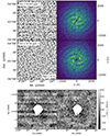 |
Fig. 4. Overview of the u = 0 flagging procedure. The top row shows a 100-channel binned empty map with horizontal stripes of one target scan of a NGC 1566 observation on the left, and on the right the corresponding FFT amplitude image, which shows a prominent vertical RFI feature at u = 0. The middle row shows the same plots, but after removal of the u = 0 stripe using our flagging procedure. The bottom row shows two zeroth-moment H I maps of NGC 1566, both created using a simple 2σ intensity cut. The bottom-left panel shows the map with the u = 0 RFI still included. The bottom-right panel shows the same map but with the u = 0 RFI removed. |
The u = 0 artefacts have been seen before in observations taken with different arrays (e.g., Hess et al. 2015; Lucero et al. 2015; Heald et al. 2016). Generally, the solution has been to simply flag a small range around u = 0 for the relevant range in v. Applying these strategies to the MHONGOOSE data would, however, result in flagging close to ∼10% of the data, due to the large number of short baselines in the MeerKAT array and the resulting high filling factor of the inner uv plane. Such a solution is clearly not ideal, and we therefore developed a more sophisticated flagging strategy (Maccagni et al. 2022) as described below.
We first split the observation into the separate target scans of ∼55 min each, and then perform the following procedure on a scan-by-scan basis. Since in each scan the uv-coverage is different, we calculate the amplitude image of a Fast Fourier Transform (FFT) of the sum of 100 line-free channels in a custom-made data cube of each scan. We adopt a pixel size of 20″ and an image size of 8000″. This leads to a pixel size of 25.8λ in the FFT image. The u = 0 artefacts are then visible as a vertical stripe (u = 0 for a range in v) in the amplitude image. We found that using an empty data cube created using a robust value of 1.5 combined with a 60″ tapering as the basis for the FFT image gave the best results.
We determine the median absolute deviation (MAD) of the distribution of amplitudes ai in the uv-plane, where MAD = median(|ai, (u, v) − median(ai, (u, v))|). We then define a cutoff threshold (median(ai, (u, v))+M × MAD), where M = 100, 150, 200, 300, 500. For each M, we find the pixels in the amplitude image where the value is larger than the cut-off and we flag the corresponding visibilities in the measurement set of that scan.
The empty cube is then reimaged and the noise measured. We adopt the value of M that gives the lowest noise and identify the corresponding flagged pixels in the amplitude image. Flags are extended by 1 pixel in u and 2 in v and the corresponding visibilities are flagged, but this time throughout the entire spectral range of the measurement set of that scan. Doing this for all scans in an observation results in removal of the u = 0 artefacts at the cost of flagging typically only a few tenths of a percent of the visibilities. This u = 0 flagging solution has been implemented in CARACal. We refer to Maccagni et al. (2022) for further information on the flagging fraction and its sky distribution.
5.5. Time flagging
The initial flagging steps removed most of the RFI in the data. However, we found that in some cases the “wings” (i.e., ramp-up and ramp-down) of time-variable strong RFI were not removed entirely. The most effective way to remove these was by using a separate time-flagging step. This was done with the CASA flagdata task (again within CARACal) where we average in bins of 100 channels, and use the tfcrop algorithm to fit the data in the time dimension and remove outliers that deviate more than 5 times the standard deviation from the fit. After merging with the initial pipeline flags, these flags are then extended such that if more than half of the visibilities at a certain observing time are flagged, all data at that time are flagged. Similarly for the frequency channels: if more than half of the data in a frequency channel are flagged, then all data at that frequency are flagged. These final flagging steps complete the reduction of a single-track observation and the individual measurement sets are now ready to be combined and for the full-depth data cubes to be created.
5.6. Standard resolutions
MeerKAT is capable of producing high-quality images over a large range in angular resolution (Fig. 1), resulting in mapping of compact, high-column density sources, as well as extended, low-column density features (Fig. 2). It is difficult to capture this wealth of structure in a single data cube at a single resolution. For MHONGOOSE, we have therefore defined six standard resolutions for our data products, which cover the angular resolution range of MeerKAT as indicated in Fig. 2.
These different resolutions are achieved by changing the robust weighting parameter used in creating the data cubes, and, for the two lowest resolutions, some additional tapering. We find that these six standard combinations give a comprehensive overview of the H I morphology and kinematics of the sample galaxies.
Table 4 and Fig. 5 show the average noise per channel and beam size as derived from the full-depth standard cubes of ten galaxies available at the time of writing. We also list the column density sensitivities where we give the values for 1σ over a single channel, as well as the 3σ over 16 km s−1 values used in Fig. 2. Finally, we also list the 3σ H I mass detection limit for an unresolved source, assuming a distance of 10 Mpc (the median distance of the galaxies in the sample) and a velocity width of 50 km s−1.
Standard resolutions.
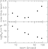 |
Fig. 5. Sensitivities of the full-depth data cubes. The top panel shows the average noise per 1.4 km s−1 channel for the six standard resolutions, as averaged over full-depth observations of ten galaxies (cf. Fig. 1). Error bars show the rms difference in noise levels between the ten galaxies, but are generally comparable to or smaller than the symbol size. The bottom panel shows the 3σ, 16 km s−1 column density sensitivities. These are the same points as shown in Fig. 2. |
The highest resolution of ∼8″ is achieved using a robustness parameter of zero. Decreasing the robustness parameter even further to negative values resulted in too small a decrease of the beam size to justify the loss of sensitivity. This loss is due to the relatively small number of longest baselines (cf. Table 3). Emphasising these through weighting does therefore not result in an improvement in image quality at these resolutions. For the purpose of MHONGOOSE H I imaging, a robustness parameter of zero therefore yields the highest usable resolution.
On the opposite end of the resolution range, tapering beyond ∼90″ does not yield additional gains due to the absence of sufficiently short baselines (cf. Table 3). This can be seen by the upturn in the noise curve at large resolutions in Fig. 1 and the top panel in Fig. 5.
5.7. Creating the full-depth cubes
For the full-depth observations, we combine the ten individual 5.5h observations and create data cubes measuring 1.5 ° ×1.5° with a velocity range from −500 km s−1 to +500 km s−1 with respect to the central velocity of the target galaxy. We choose to image an area larger than the usual primary beam of ∼1° due to the high sensitivity of the observations, which enable H I detections at a large distance from the pointing center.
The ten input observations were first all corrected from a topocentric spectral coordinate grid to a common heliocentric spectral grid. We adopt the radio velocity definition where all channels have a constant frequency spacing and velocity is defined as vradio = c(ν0 − ν)/ν0, where ν0 is the rest-frequency and ν the observed frequency. The ten measurement sets were then all simultaneously input into wsclean (Offringa et al. 2014) to create and deconvolve the final data cubes. So-called “clean masks” were used to indicate areas with emission where deconvolution was necessary. These masks were created automatically using a sequence of cubes at each of the standard resolutions listed in Table 4.
Starting at the lowest resolution r10_t90, we created an initial deconvolved cube (cube_0) using the auto-masking option in wsclean, where the mask (mask_0) was defined to include values of 5σ and higher. We then used SoFiA-2 (Westmeier et al. 2021) outside of CARACal to create a new mask (mask_1) based on the deconvolved cube_0.
Here, and for all subsequent SoFiA-2 runs, we used spatial kernels of 0 and 3 pixels, and velocity kernels of 0, 3, 7 and 15 channels. Using the smooth-and-clip (S+C) method (Serra et al. 2012), we used a threshold of 4σ to define the mask with spectral noise scaling enabled. To define sources, valid pixels were linked across a maximum spatial and spectral distance of, respectively, 3 pixels or 3 channels. For the detected sources we then imposed a spatial minimum size equal to the current beam size rounded up to the nearest integer number of pixels. For the spectral minimum size, we used 10 channels (14 km s−1). Sources with negative flux density values were not retained. These SoFiA-2 input parameters were extensively investigated to ensure that they optimally captured the emission present in the cubes.
The resulting mask_1 was used to create and deconvolve a new cube_1. A new run of SoFiA-2 on this cube resulted in a mask_2, which was in turn used to create cube_2, which is the final deconvolved r10_t90 cube. Within the masks, emission was deconvolved down to 0.5σ. The gain value for the major iterations in wsclean was set to 0.95 to ensure at least one cycle of inversion of the clean model to visibility space.
For subsequent, higher spatial resolutions, the final mask of the previous, lower resolution run was used as the initial mask. That is, for the r05_t60 cubes, the final mask_2 of the r10_t90 run was regridded and used as the initial mask_0 of the r05_t60 runs.
The procedure is then as above where a cube_1 is produced and SoFiA-2 is run on that cube to build a mask_1. This is then used to create and deconvolve the final cube_2.
This is then repeated in sequence for each of the resolutions, where the final mask of a given resolution is used as the initial mask of the next higher resolution. This process is a fully automated part of our reduction pipeline. It delivers high-quality deconvolved cubes almost entirely unsupervised.
As expected, the noise in the data cubes keeps decreasing as the square root of the integration time as each of the ten observations is added in turn. This is illustrated in Fig. 6 where we show the noise per channel measured in natural-weighted data cubes of ESO 300-G014 (J0309–41), created by combining an increasing number of tracks. We used natural weighting, instead of one of the standard resolutions, to circumvent uncertainties due to changes in the noise because of weighting and tapering and to enable an unambiguous comparison with the expected theoretical noise. The latter is calculated based on the number of visibilities and the properties of the MeerKAT antennas (13.5m dishes and Tsys/η = 20.5 K) and is also shown in Fig. 6. The theoretical values have (by definition) a slope of −0.5. The measured values have a slope of −0.504. The very small offset between the lines is equivalent to an offset in Tsys/η of ∼0.4 K, in the sense that MeerKAT performs slightly better than our assumptions (though such a small offset is likely to be within the variations between different observations).
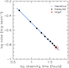 |
Fig. 6. Natural-weighted noise values measured over a 1.4 km s−1 channel as a function of integration time for the observations of ESO 300-G014 (J0309–41). The black filled points indicate the measured noise level. The blue line shows the expected theoretical noise levels with a slope of −0.5. A linear fit to the observed noise levels gives a slope of −0.504. The red star indicates the target sensitivity from de Blok et al. (2016). |
The measured noise level thus meets the requirements presented in the MHONGOOSE white paper (de Blok et al. 2016), where a noise level of 0.074 mJy beam−1 per 5 km s−1 channel after 48 hours of on-source is specified. Scaling this to the channel width and observing time that were eventually used, we see an almost exact match, as indicated in Fig. 6, showing that the full-depth MHONGOOSE data are of the required sensitivity to deliver the envisaged survey science.
5.8. Creating full-depth moment maps
We also create zeroth-, first- and second-moment maps showing the integrated H I distribution, the intensity-weighted mean velocity and the velocity width, repectively.
The second-moment map is commonly referred to as a velocity dispersion map. However, strictly speaking, second-moment values only represent a physically meaningful velocity dispersion in cases where the H I emission line profile is well approximated by a single Gaussian2. In all other cases (non-Gaussian profiles or multiple separate components) they simply quantify the spread of H I velocities along each line of sight.
We used SoFiA-2 to find the signal in the cubes and create the masks. The S/N in the cubes is high, and we found that we only needed a limited number of spatial kernels to isolate the signal. In fact, using spatial kernels larger than ∼1–2 beam sizes had the effect of introducing additional noise into the moment maps at the edges of the disks and these larger kernels were therefore avoided. We used cubes that were not corrected for the primary beam. This correction was applied to the zeroth-moment maps afterwards.
The SoFiA parameters we eventually used were spatial kernels of 0 and 4 pixels and velocity kernels of 0, 9 and 25 channels using a source-finding S+C threshold of 4σ. Sources were linked over a maximum of 5 pixels spatially and 8 channels spectrally. Minimum sizes of 4 spatial pixels and 15 channels were imposed.
We then used the reliability parameter, as implemented in SoFiA, to further separate signal from the noise. We did find, however, that this parameter was less critical as almost all sources were well separated from the noise and an integrated S/N cut was usually sufficient to identify the significant sources. In our case, we mostly used a reliability value of 0.8 and an integrated S/N value of 5.0.
The masks as defined here are stricter than the masks used during deconvolution. This is due to the different purpose that they serve. The deconvolution masks were created to include all emission at many scales, even if this leads to including some noise in the masks. For the moment maps, instead, it is important that as little noise as possible is included in the masks to avoid affecting the moment values.
5.9. Examples of full-depth moment maps
A full scientific analysis of the full-depth data will be presented in forthcoming papers. For this reason, and as data are still being collected, we restrict ourselves here to presenting a short overview of the full-depth data for two of the galaxies that were completed early in the survey. We refer to Healy et al. (2024) and Maccagni et al. (2024) for in-depth discussions. The purpose of this overview is to give an indication of the high quality of the data.
Figure 7 shows multi-resolution maps of the H I distribution in NGC 1566 (J0419–54) and NGC 5068 (J1318–21). Here we show for five of the six standard resolutions the contour at the column density level that corresponds to S/N = 3 in the zeroth-moment map at that resolution.
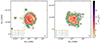 |
Fig. 7. Multi-resolution zeroth-moment maps of NGC 1566 (left panel) and NGC 5068 (right panel) based on the full-depth data. For each resolution, contours of 2n times the S/N = 3 value are shown (as listed in the legend). The resolutions shown are r05_t00 (red), r10_t00 (green), r15_t00 (blue), r05_t60 (purple), r10_t90 (olive). For each resolution two contours are shown, i.e., n = 0, 1, except for the highest resolution r05_t00 (red contour), where n = 0, 1, 2, … The r05_t00 moment map is shown in the background as a false color image, with the column density levels indicated by the color bar on the right. The beam sizes (colored according to the respective resolution) are shown in the bottom-right corner. |
During the initial reduction procedure, the velocity channels were not Hanning-smoothed and binned in velocity every two input channels (cf. Sect. 5). The channels in the current data cubes are therefore independent, meaning that the noise is expected to behave as  when summing N channels.
We therefore can construct a noise map with pixel values defined as  , where σchan is the average noise value measured in empty channel maps, δv is the velocity width of a channel (in this case 1.4 km s−1) and N is the number of independent channels contributing to each pixel in the zeroth moment map.
Taking the ratio of the zeroth-moment map and this noise map then gives a S/N map. We derive the median column density value of all pixels with 2.75 < S/N < 3.25 and adopt this as the column density corresponding to S/N = 3 (also known as the “pseudo-3σ” column density; see Verheijen & Sancisi 2001; Kregel et al. 2004).
We plot contours of multiples of this value, thus clearly capturing in a single figure the detailed, compact high-column density distribution at the highest resolutions, and then transitioning into the diffuse, extended distribution of the low-column density H I at the lowest resolutions. Note the extended and irregular distribution of H I in the outer parts of NGC 1566, as well as the clumpy outer H I in NGC 5068. At column densities of ∼1020 cm−2 (corresponding with the edge of the main star-forming disks) very little of this irregular outer H I would be detected and both galaxies would give the impression of regular, symmetric disks; cf. the observations of NGC 1566 in Elagali et al. (2019) which concentrated on the high-column density disk. As we show below, the outer H I components contain only a small fraction of the total H I mass of the galaxies, but they dramatically change the apparent morphology. As mentioned, more extensive analyses of these and other sample galaxies will be presented in future papers, but Fig. 7 already shows the power of these deep observations.
5.10. Single-track moment maps
Observations are still ongoing at the time of writing, and full-depth observations are not yet available for the entire sample. However, every galaxy in the sample has by now been observed for at least one 5.5h track. The results presented in the remainder of this paper are based on the single track data, unless otherwise stated. To give an overview of the sample and pursue initial sample-wide science, we created single-track moment maps at two of the standard resolutions r05_t00 and r15_t00 (beam size of ∼12″ and ∼30″, respectively) in an identical manner as for the full-depth data. We have limited this to two resolutions as the differences between the standard resolutions are not as pronounced here due to the ten times shorter integration time. Average beam sizes for these single-track observations are identical to those listed in Table 4, while column density and mass limits are a factor  less (cf. Fig. 6). These moment maps give a comprehensive overview of the entire MHONGOOSE sample as observed by MeerKAT.
In Fig. 8 we show the r05_t00 single-track moment maps for NGC 1566 (J0419–54) and NGC 5068 (J1318–21) which were also discussed in Sect. 5.9. In the Figure, we show the Dark Energy Camera Legacy Survey (DECaLS)3 (Dey et al. 2019) optical image, the zeroth-moment (integrated H I intensity) map, the first-moment (intensity-weighted mean velocity field)4 and finally, the second-moment map. For both the first- and second-moment maps, pixels corresponding to values below the S/N = 3 column density in the zeroth-moment map were blanked. A comparison between Figs. 7 and 8 for these galaxies clearly show the improvement in sensitivity that we can expect from the full survey.
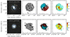 |
Fig. 8. Example single-track moment maps using the r05_t00 resolution for two MHONGOOSE galaxies. Top row: NGC 1566 (J0419–54); bottom row: NGC 5068 (J1318–21). From left to right: (i): Combined grz-color image from DECaLS. (ii): Primary-beam corrected zeroth-moment or integrated H I intensity map. Contours as indicated in the figure. The lowest contour represents S/N = 3, with subsequent contour levels increasing by a factor of two. (iii): First-moment map or intensity-weighted velocity field. Red colors indicate the receding side, blue colors the approaching side. The central velocity (listed in Table 1) is indicated by the thick contour. Other contours are spaced by 10 or 20 km s−1, as indicated in the Figure. (iv): Second-moment map: colors show the range from 0 (light-blue) to 30 (red) km s−1. The lowest contour shows the 12 km s−1 level, and subsequent contours are spaced by 12 km s−1. The 24 km s−1 contour is shown in black. For both the first- and second-moment maps, pixels corresponding to values below the S/N = 3 column density in the zeroth-moment map were blanked. See Appendix A for a more extensive description. |
Moment maps for the r05_t00 resolution of the complete sample are given in Appendix A and we refer to this Appendix for a more extensive description.
6. Global H I profiles
The global H I profile or integrated H I spectrum of a galaxy shows the spatially integrated H I flux density as a function of velocity or frequency. It is often used in scaling relation studies, such as the Tully-Fisher relation (Tully & Fisher 1977) and also in studies involving the total H I masses of galaxies. Global H I profiles are often measured using single-dish telescopes. These measure the total power, and therefore the total H I mass. Global H I profiles measured with synthesis radio telescope arrays are less straight-forward to interpret. Depending on the baseline distribution of the array and the extent of the source, these may suffer from the so-called “missing spacing” problem, which is caused by a lack of short baselines which prevents measurements of flux on larger angular scales. For galaxies that have an angular size similar or larger than the scales probed by the shortest baselines of the array this can lead to a severe underestimate of the total H I mass. In these cases, a comparison with the single-dish H I global profile is often used to determine whether any H I has been missed in the synthesis observations. For MeerKAT, with a shortest baseline of 29m, the largest scale at which signal can be detected is ∼20′.
Comparisons between the single-dish H I profiles and those derived from synthesis observations have been used to constrain the existence of low-column density H I in galaxies (e.g., Pingel et al. 2018; Kamphuis et al. 2022). The underlying assumption is that any flux not detected in the synthesis observations must be extended and/or of low column density.
MeerKAT has been specifically designed to have a compact core with many short baselines, and one may expect that any missing-spacing issue will be less severe. The MHONGOOSE data, both the single-track and full-depth observations, offer a chance to systematically compare the measured masses with single-dish masses for a significant number of our sample galaxies. Below we first compare the single-track and full-depth profiles to gauge whether the increased observing time led to the detection of additional H I. This is then followed by a comparison with the single-dish measurements.
6.1. Comparing the single-track and full-depth profiles
A first step is to compare the H I global profiles of the single-track data and full-depth data which differ by a factor of ten in observing time. This obviously means an increase in S/N for the full-depth data, but an interesting question is whether this can be used to deduce the existence of low-column density H I.
We compare the global profiles and total H I masses for ten of the MHONGOOSE galaxies for which the full-depth global profiles were determined. The global profiles are derived by measuring the flux in each channel, applying the masks that were used to create the moment maps. The fluxes are corrected for primary beam attenuation. The global profiles are compared in Fig. 9 with the corresponding flux densities (as listed in Table 5). The full-depth H I masses are on average ∼2% higher than the single-track H I masses. Such differences may sound insignificant, but they make a big difference when it comes to deducing the existence of a low-column density component.
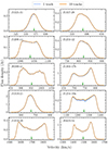 |
Fig. 9. Single-track (blue) and full-depth (orange) global H I profiles for ten of the MHONGOOSE galaxies as identified in the top left of each panel. The green arrows indicate the central velocities. We show only the velocity ranges where signal was present in the mask. |
H I mass comparison between full-depth and single-track MeerKAT observations.
If we assume that for each galaxy, the “extra” detected H I is due to a previously undetected low-column density H I component that is spread evenly over the H I disk, then we can use the additional mass and the area of the disk to calculate the column density. This results in column density components of a few times 1017 cm−2 to a few times 1018 cm−2, as listed in Table 5. This is consistent with the increase in column density detection limits going from single-track to full-depth observations. These numbers highlight that to deduce the presence or absence of low column density gas based purely on global profiles, an accuracy of a few percent or better is needed. Such an accuracy is much higher than the typical absolute flux calibration uncertainty of H I observations. This is compounded when comparing with results from different telescopes.
6.2. Comparison with single-dish profiles
Above, we show that the longer integration times of the full-depth data allow us to detect a small amount of additional H I. However, this internal comparison does not address the “missing spacing” issue. A further question is therefore whether MeerKAT is able to give us an accurate measurement of the total H I mass of our galaxies.
As the MHONGOOSE sample is ultimately selected from HIPASS, single-dish Parkes observations are available with a beam size of 15′ and flux measurements for all but one of the sample galaxies are given in the HIPASS Bright Galaxy Catalog (BGC; Koribalski et al. 2004). The one galaxy that is not in the BGC (J0429–27) falls below the flux limit of that catalog. Instead we use the flux density value as listed in the Meyer et al. (2004) HIPASS Catalogue. In addition, 15 of our galaxies have been observed with the GBT with a beam size of 9′ (Sorgho et al. 2018; Sardone et al. 2021).
We can therefore test whether the MHONGOOSE observations manage to recover the total flux. As the differences between the flux densities derived from the single-track and full-depth data are only small (as discussed above), we use the single-track flux densities here, as this maximizes the number of galaxies where a comparison can be made.
The single-track flux densities are listed in Table 6, with the velocity widths given in Table 1. These are based on the r15_t00 data using masks as described in Sects. 5.10 and 6.1. The 20% velocity width W20 is defined as the difference between the velocities where the profile reaches 20% of its peak value. The central velocity is defined to be halfway between these velocities.
MeerKAT and single-dish H I mass comparison.
We additionally list the HIPASS and GBT flux densities in Table 6 for those galaxies where at least one single-dish measurement is available. We have remeasured the GBT flux densities from the original profiles, as the values listed in Sardone et al. (2021) represent cumulative flux densities integrated over the entire respective areas mapped by the GBT, rather than direct integration of the global profiles as discussed here. The H I profiles themselves are shown and compared in Fig. 10. Where necessary we have shifted the literature spectra to the same radio velocity scale as the MeerKAT profiles. Any “peaks” detected in the single-dish data outside the velocity range of the target galaxies (e.g., the HIPASS profile of J0008–34 at v ∼ 270 km s−1 in Fig. 10) are due to noise.
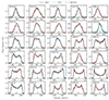 |
Fig. 10. Comparison of the MeerKAT and single-dish profiles. MeerKAT r15_t00 profiles are shown in black, GBT profiles (Sardone et al. 2021) in cyan, and HIPASS profiles (Koribalski et al. 2004) in red. The green arrows indicate the central velocties as derived from the MeerKAT data. |
In Fig. 11 we compare the MHONGOOSE, HIPASS and GBT flux densities. The HIPASS values are systematically lower than the MeerKAT and GBT values. One explanation could be that some of the H I has been subtracted during data processing by the running bandpass correction method (Barnes et al. 2001). The flux densities of H I-bright galaxies are also known to be affected by the gridding used in the HIPASS pipeline (Barnes et al. 2001; Koribalski et al. 2004).
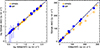 |
Fig. 11. Comparison of the single-track MeerKAT flux densities with single-dish flux densities. Stars (orange) indicate HIPASS values, filled circles (blue) GBT values. The full black line indicates a unity slope. The left panel compares the flux densities on a logarithmic scale, the right panel shows the same data points on a linear scale. The dashed blue line is a fit to the GBT points. The fit to the logarithmic GBT values has a slope of 0.968, the linear values give a fit with a slope of 0.954. The dotted orange line is a fit to the HIPASS data. Here the logarithmic slope is 0.964, the linear fit gives a slope of 0.860. |
The agreement with the remeasured GBT flux densities is good. The ratio of the GBT and MeerKAT flux densities is 1.058 ± 0.080, so the GBT on average detects ∼6% more flux, but this is within the scatter of ∼8%. A least-squares fit to the linear values, as shown in Fig. 11, has a slope of 0.964, but this slope is mainly determined by NGC 7424 (J2257–41), the galaxy with the largest flux density, where we find that the GBT actually detects less H I than MeerKAT. Leaving that point out we end up with a slope of 0.997, again indicating good agreement between the MeerKAT and GBT fluxes. This is especially so when one considers the uncertainty in the MeerKAT flux calibration of ∼10% (Serra et al. 2023) and a most likely similar uncertainty in the GBT flux calibration. The good agreement is consistent with the fact that most sample galaxies are significantly less extended than the ∼20′ maximum angular scale that the MeerKAT shortest baseline of 29m is sensitive to.
7. Comparing the moment maps
7.1. Pixel-pixel density histograms of individual galaxies
The moment maps presented in Fig. A.1 give an overview of the morphology and kinematics of the H I in the MHONGOOSE galaxies. In terms of column density sensitivity these single-track observations approach the sensitivity of the HALOGAS survey to within a factor of two (cf. Fig. 2, shifting the MHONGOOSE line up by 0.5 dex).
An efficient method to further summarize this information is pixel-by-pixel scatter plots of the various moment values: for each location (pixel) the value of one moment is plotted against that of a different moment at that same location. A number of previous studies have used these plots to study properties of galaxies. For example, de Blok et al. (2018) used the distribution of the zeroth- and second-moment values of the H I distribution in the M81 triplet to find that each of the three triplet galaxies occupied unique positions in that particular parameter space, and addressed the question of whether the M81 triplet could be the equivalent of a Lyman-α absorber (cf. their Fig. 20). Maccagni et al. (2021) presented optical line emission data of Fornax A and used the distribution of zeroth- and first-moment values to distinguish between rotating and outflowing gas. Sun et al. (2018, 2020) studied the zeroth and second moments of the CO distribution in the Physics at High Angular resolution in Nearby GalaxieS (PHANGS) galaxies.
The single-track MHONGOOSE observations give us the opportunity to do a similar analysis for 30 galaxies in H I, with all of them observed and reduced in an identical, homogeneous manner. Here we explore the relation between column density and velocity width (zeroth and second moment).
We use the r15_t00 data of all of our galaxies and plot the zeroth- and second-moment map pixels of each of our galaxies against each other. The ∼30″ resolution data gives a good column density sensitivity while not greatly sacrificing angular resolution (cf. Fig. 5). We realise that the individual pixels are not independent of each other. However, here we only consider the relative distributions at a single resolution. Taking the size of the beam into account would only change the absolute scaling.
Rather than using scatter plots where subtle differences are often difficult to make out, we derive a two-dimensional density histogram covering the column density-velocity width parameter space with a 75 × 75 grid.
The zeroth-moment values are corrected for inclination and converted to surface densities by multiplying them by cosi, where we assume the inclinations given in Table 1. We found that this simple correction was sufficient for our purposes, with conclusions insensitive to the exact inclinations values.
The panels in Fig. 12 show, for each galaxy, the number of pixels having values corresponding to any given combination of column density (horizontal axis) and velocity spread (vertical axis). This is shown as a two-dimensional density-histogram with each bin having the value given by the color scale for that panel. Bins are only shown if there are a minimum of four moment pixels falling in them. The contours show a similar density histogram but in this case derived from all the single-track moment maps of all galaxies combined. The juxtaposition of the two distributions allows for a quick comparison of the distribution for a particular galaxy with that of the entire sample. This total distribution is further discussed in Sect. 7.2.
To highlight any differences between galaxies of different masses, we divide the galaxies in three equal-number bins in rotation velocity, as shown in Fig. 12. The rotation velocities are calculated from the W20 and i values given in Table 1. Within each rotation velocity bin we show the galaxies in order of increasing inclination.
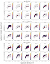 |
Fig. 12. Two-dimensional density histograms showing the distribution of inclination-corrected column densities and second moment values for the MHONGOOSE galaxies. Each histogram consists of 75 × 75 hexagonal bins, and only bins containing more than 4 pixels are shown. The color bar on the right in each panel indicates the number of pixels per bin. The background contours indicate the total distribution of the entire sample as shown in Fig. 13. Galaxies are divided in three bins in rotation velocity. Within each bin, galaxies are ordered by increasing inclination, with the most face-on galaxies in the top-left, and the most edge-on in the bottom-right. The two light-gray bars between the panels in each bin indicate inclinations of 50° (b/a = 0.67) and 70° (b/a = 0.33), respectively. |
We see a large spread in the typical second-moment values for each galaxy. Compare for example the high values found in J1318-21 with the low ones in J0351-38. While our galaxies have a range in distance, this is not the cause of the spread in these typical values (which would be due to the beam measuring a larger number of kpc for more distant galaxies, and thus potentially capturing a larger range in velocities). The main determining factor seems to be the SFR. We discuss this further below.
In the highest-rotation velocity bin we can make out a number of interesting trends. The lowest inclination galaxies in general cover most of the parameter space as traced by the entire sample. The only exception is J2257–41 which has low second-moment values. Moving to the high-inclination galaxies we see that they exclusively cover the upper part of the diagram. This is not a beam-smearing effect, but is rather caused by the longer line-of-sight through the disk, resulting in increased linewidths. We refer to Appendix B for a more in-depth discussion of the impact of beam smearing and inclination.
The face-on massive galaxies show significantly increased second-moment values at the highest column densities. While some of this will be due to beam smearing in combination with a steeply rising inner rotation curve, part of it will be intrinsic to the galaxies. Most of these high values occur in the central parts of the galaxies and are likely related to the intense star formation in these portions of the galaxy. They mark the presence of winds or outflows powered by star formation or an AGN. The most massive galaxies in the sample, NGC 1566 (J0419–54), NGC 1672 (J0445–59), NGC 1371 (J0335–24) and NGC 289 (J0052–31), are known Seyfert galaxies.
The lowest-rotation velocity galaxies do not show these extreme second-moment values, but rather cling to the bottom of the distribution for the lower inclinations, though we do see larger second-moment values towards the more edge-on galaxies.
The situation for the intermediate rotation velocity galaxies is complex. We do not see a clear trend of the distribution changing with inclination. An extreme example is NGC 5068 (J1318–21) which shows the highest second-moment values in this bin, yet is the most face-on galaxy. The complex situation in this galaxy is described in more detail in Healy et al. (2024). Another complex distribution can be seen for NGC 1705 (J0454–53). This is a starbursting dwarf galaxy, and the parallel track of high second-moment values are indications of the gas outflows in this galaxy (cf. Meurer et al. 1998). A few more of these intermediate-rotation velocity galaxies show multiple velocity width values at a given surface density. In many cases the high second-moment values are linked to locations where there are multiple components along the line of sight due to, e.g., spiral arms, the presence of extra-planar gas, or long lines of sight through the disk.
An in-depth analysis of these density histograms, with the addition of information on the distribution of molecular gas, such as presented in Sun et al. (2018, 2020), will give much information on the conditions for star formation in nearby galaxies and the link with the properties of the atomic and molecular gas. Such a quantitative analysis is, however, beyond the scope of this paper.
7.2. Total pixel-by-pixel density histogram
We now consider the surface density-velocity width density histogram of the entire sample. Here we again use the same 75 × 75 grid to sample the displayed parameter range, but only display bins containing more than eight sample values. This integrated histogram is shown in Fig. 13 and contains several interesting features. Some of these are known from the literature, but others have not been explicitly noted before.
 |
Fig. 13. Two-dimensional density histograms showing the distribution of zeroth and second moment values for the entire MHONGOOSE sample. The histogram consists of 75 × 75 hexagonal bins, and only bins containing more than 8 pixels are shown. The color bar indicates the number of pixels with the H I column density and velocity widths indicated by the horizontal and vertical axes, respectively. |
At the highest column densities we see a steep drop-off in the density distribution, despite this being the part of the diagram with the highest S/N. This drop-off occurs at surface density values of log(NH I/cm−2) ∼ 21.1, or ∼10 M⊙ pc−2, and thus implies an upper limit to the H I column density (at this resolution). This value agrees well with the upper limit of ≈9 M⊙ pc−2 found by Bigiel et al. (2008) for the THINGS sample at similar resolutions (also see Leroy et al. 2008; for a more detailed observational view, see Schruba et al. 2017). A comparison with molecular gas column density values shows that this upper limit corresponds with a transition from an atomic to a molecular ISM (cf. Krumholz et al. 2009; McKee & Krumholz 2010; Sternberg et al. 2014).
Turning to the second-moment values, we see that at surface densities log(NH I/cm−2) > 19.5 there is a well-defined lower limit to the second-moment values. This limit occurs at ∼8.5 km s−1. Given the 1.4 km s−1 velocity resolution of the data (corresponding to the lower limit of the plotted second-moment range) and the high S/N of the profiles in this part of the diagram, this cannot be a velocity resolution artefact but must indicate an absence of H I profiles with second-moment values less than ∼8.5 km s−1. To first order, the ISM is considered to consist of a cool neutral medium (CNM) with a temperature of a few tens of K and a warm neutral medium (WNM) with temperatures around ∼8000 K . The CNM line profiles have a line width of ∼1 km s−1 while WNM line width are ∼8 km s−1 (in the absence of any other processes that can broaden line-widths) (Braun 1997; Wong & Blitz 2002; Wolfire et al. 2003). The lower limit found in our data does not indicate an absence of CNM, but merely shows that the H I emission, and therefore the line width, is dominated by the WNM, where the latter has a lower limit to its observed velocity dispersion as shown in Fig. 13.
As is evident from Fig. 12, many of the galaxies show distinct local density concentrations in the histograms. We also see this in the total density histogram, suggesting this is a general feature of our sample. Figure 13 shows a local maximum in the combined distribution centered on log(NH I/cm−2) ∼ 20.6 and another (less concentrated) one around log(NH I/cm−2) ∼ 19.5. Comparison with the integrated H I maps as well as SINGG Hα and GALEX UV images shows that the profiles corresponding to the high-column density concentration are generally found in the star-forming disks of the galaxies. The profiles contributing to the low-column density concentration are generally found in the outer disk or in inner disk regions with little to no detected star formation as seen in the Hα and FUV images. The high-density clump in Fig. 13 also shows a “tail” at high velocity dispersion, which is not visible in the low density clump, possibly induced by feedback from star formation.
Perhaps the most interesting is the clear division between these two concentrations around log(NH I/cm−2) ∼ 20.3 (NH I ∼ 2 × 1020 cm−2). If H I complexes gradually collapse either under their own gravity or triggered by an external event, we would expect the observed H I column density to continuously increase, and therefore expect to see a continuous H I column density distribution in Fig. 13. If we assume that collapsing H I complexes move from left to right in the Figure (i.e., from low- to high-column density), then the presence of the division points to a short timescale for this column density increase.
A possible explanation for the presence of this division is related to the formation of the CNM. This was put in a physical context in Kanekar et al. (2011). Based on measurements of the spin temperature in a large number of Galactic H I clouds they identify a rapid change in spin temperature at ∼2 × 1020 cm−2. They associate this with a threshold H I surface density for formation of the CNM. Above this ∼2 × 1020 cm−2 threshold, the H I can sufficiently self-shield against UV photons to enable formation of a cool component. Below this threshold the UV photons can heat and ionize the gas, preventing the formation of a CNM. Note that this threshold also corresponds to that used to define a Damped Lyman-α system.
Following the interpretation by Kanekar et al. (2011), these data show that the existence of a CNM, which is more closely associated with star formation, leaves an imprint on the moment maps, including a rapid transition to higher column densities once this component starts forming. Figure 13 thus shows, in a single plot, the various transitions occurring towards star formation. At the lowest column densities, between ∼1019 and ∼1020 cm−2, the gas is dominated by the WNM, and there is little or no star formation (Bigiel et al. 2010; Serra et al. 2012; Maccagni et al. 2017). At ∼2 × 1020 cm−2 the gas is sufficiently dense that a significant CNM can rapidly develop. The approximate column density limits of the high-column density concentration correspond closely to the values given in Bigiel et al. (2010) (∼3 − 10 M⊙ pc−2 or log(NH I/cm−2) ∼ 20.5 − 21.1) where star formation is efficient.
We expect that the CNM will still be embedded in a WNM (at the resolution of our observations), where the WNM is the source of the observed second-moment values. We therefore do not see the lower CNM velocity dispersions reflected in the plot, but studies of the individual profiles should provide clear evidence for its presence. The gas turns completely molecular at the column density cut-off discussed above.
It will be interesting to repeat this analysis once all full-depth data are available. The increase in S/N will allow exploration at different angular resolutions, but also, perhaps more crucially, at identical physical resolutions.
7.3. Masking and moments
One of the distinct features in Figs. 12 and 13 is the tail of decreasing second-moment values towards low surface densities. Naively, one might presume that this could be a consequence of the low-column density gas being mostly in the outer disk where there is less energy available to heat and stir up the gas, leading to a low velocity dispersion. The true cause is more prosaic, however, as we show here that it is caused by the masking procedure used to create the moment maps.
The SoFiA-2 moment map creation steps described above are a sophisticated combination of source finding and masking at different spatial and velocity scales. The essentials of this can, fortunately, already be captured by considering an idealized Gaussian H I profile with constant velocity dispersion and variable normalisation or peak value (corresponding to different column densities).
We consider a data cube with a noise per channel σch in which we embed Gaussian line profiles with a fixed velocity dispersion and a peak value expressed as some multiple of σch. Analogous to our SoFiA moment map construction, we assume that we mask the data at the 4σch level. For a Gaussian with a peak close to the noise level most of the profile will be masked, while a high S/N profile will be much less affected.
We consider the second moment of the remaining > 4σch profile after masking as a function of the S/N of the profile. Without masking (and for noise-free data), this would equal the velocity dispersion of the Gaussian. With masking, it decreases as the peak value decreases.
A second effect is that the area underneath the masked Gaussian (the zeroth-moment value or integrated flux) also decreases after masking due to removal of the high- and low-velocity wings of the profile. This also causes a relatively larger decrease in column density as the peak flux density declines.
In Fig. 14, we plot the curve showing the calculated changes in the measured zeroth- and second-moment values for a single fixed-velocity dispersion Gaussian as a function of its peak value and superimpose this on the surface density-velocity width density histogram. The absolute vertical position of the curve is determined by the input velocity dispersion of the Gaussian. The horizontal position of the curve is fixed by identifying the typical S/N for a given column density. In Fig. 14 we show the resulting changes for a Gaussian masked at 4σch with a velocity dispersion of 10 km s−1, and a S/N of 1000 for a column density of 1021 cm−2. This is approximately correct for the data shown here, as deduced from the S/N maps discussed in Sects. 5.8 and 5.10. We show two models in Fig. 14, one where we ignore the decrease in flux due to masking, and one where we do take this into account. The latter extends to lower column densities.
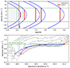 |
Fig. 14. Illustration of the change in zeroth- and second-moment values due to masking. The top panel shows a number of Gaussians, here plotted as a function of velocity as given by the vertical axis, while the horizontal axis indicates the peak value of the Gaussian in terms of S/N. From right to left the peak values are 1000, 100, 50, 10 and 5 times the S/N. The dashed vertical black line indicates the 4 times S/N level where masking occurs. Each profile has a velocity dispersion of 10 km s−1 as indicated by the horizontal dashed green lines, and, for each Gaussian separately, the dotted vertical green lines. The thick red lines indicate the measured second-moment values for each Gaussian, assuming they are masked at 4 times the S/N. The bottom panel shows the change in zeroth and second moment values. Here we have lined up the positions of the peaks in the top panel with those of the points in the bottom panel by assuming that a column density of 1021 cm−2 corresponds to a S/N of 1000. This is consistent with the data presented in Fig. 13 that are shown here as contours. The curve extending to the left (open circles) takes into account that the total flux of the Gaussian decreases due to masking, the right-hand curve (closed circles) ignores this. For other assumed velocity dispersions, the shape of the curve does not change but will shift up (larger dispersions) or down (lower dispersions). |
For the assumptions made here, the shape of this relation is fixed. Changing the input velocity dispersion merely shifts it up and down, while increasing the S/N of the underlying data would shift it horizontally. The tail towards lower column densities is therefore an unavoidable byproduct of the masking procedure. Longer integrations (i.e., a decreasing noise) would push the tail to lower column densities. A similar analysis using full-depth cubes would result in the tail starting at column densities that are  , or 0.5 dex lower in column density.
Note how well the down-turn in the tail is described by the simple single Gaussian model. We can deduce for the masking procedure described here that at S/N values between ∼50 and ∼10, the second moment values start to underestimate the velocity dispersion. At a S/N ∼ 5, the second moment underestimates the velocity dispersion by a factor of ∼2.5. Column densities, though not as affected, can nevertheless be underestimated by factors of ∼1.6 at these lower S/N values. Multiple components along the line of sight will not significantly influence the lower bounds of the distribution as, at a given column density, these will be found at higher second-moment values. Nevertheless, fitting multiple Gaussians to the velocity profiles could further elucidate (or better: circumvent) the effects of masking in the presence of multiple profiles.
In short, in our specific case of masking at 4σ, moment values below a S/N ∼ 20 should be used with care, as these will introduce significant biases with respect to the true column density or velocity dispersion. Different masking levels and methods produce different S/N level limits, but the general conclusion remains and will always be relevant when masking is used. As noted, deeper data cannot totally remove this this issue, but will shift these effects towards lower column densities.
8. Other galaxies in the MHONGOOSE fields
The sensitivity and large field of view of MeerKAT result in the detection of additional companion and field galaxies. Here we give a first inventory of the galaxies detected in the 1.5° by 1.5° single-track fields in a velocity range of −500 to +500 km s−1 with respect to the central velocity of the target galaxies. Detections are based on the single-track zeroth-moment maps. A list of these additional galaxies is given in Table 7. For the fields where additional galaxies are present, Fig. 15 shows the positions of these galaxies. We expect an even larger number of galaxies to be detected in the full-depth data once available. While the search volume is defined with respect to our target galaxies, this does not imply that every one of these additional galaxies is also physically associated with those target galaxies. Most of them will be, but it is possible that (especially at the edges of the volume probed) we are picking up some foreground or background galaxies.
Additional galaxies in the field.
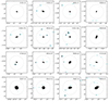 |
Fig. 15. Overview of the zeroth-moment maps of the fields where additional galaxies are present. The HIPASS name of the target galaxy (center) is identified in the top-right corner of the zeroth-moment maps. The additional galaxies are indicated by blue circles and their properties are listed in Table 7. A small number of galaxies are not indicated as they partially fall outside of the field of view shown here. The large dotted circles indicate a diameter of 1 degree, equivalent to the FWHM of the MeerKAT primary beam. The maps have been corrected for primary beam attenuation. |
The Table reports a variety of integrated H I properties, as well as the identification of the optical counterparts. These identifications were made by consulting the SIMBAD and NED data bases. We find that half of the additional H I detections can be definitively associated with an optical counterpart through a match both in position (generally to within one or two beams) and in velocity (generally to within a few tens of km s−1). Most of the other half can be reliably associated with an optical counterpart through a position match only, because no previously measured velocity is noted in either the NED or SIMBAD databases, and our redshifts are the first ones measured for these objects. Finally, we find four galaxies (indicated with the MKT prefix in Table 7) that have no previous identification, but where an optical counterpart is clearly visible in DECaLS images.
Three additional galaxies visible in the moment maps are partially outside of the volume of the data cubes used here. These are LEDA 583148 in the J0309–41 field, ESO 486–21 in the J0459–26 field, and MKT J125225.4-124304.1 in the J1253–12 field. For these three galaxies we list the position and approximate radial velocity in Table 7. We refrain from presenting their H I line widths and fluxes because the large uncertainty due to the incomplete coverage by the data used here. The last of these three galaxies is a fifth, previously uncataloged galaxy. All of the additional galaxies listed here can thus be associated with an optical counterpart; we have not found any “dark” galaxies.
We note that one of our lowest H I mass galaxies, UGCA 15 (J0049–20), is itself a companion to the larger galaxy NGC 247. This is the only case where a “companion” galaxy is more massive than the target galaxy and we do not include NGC 247 in the following analysis.
Figure 16 shows the integrated H I maps overlaid on optical DECaLS images along with the global H I profiles (corrected for the primary beam) of the additional galaxies.
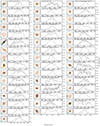 |
Fig. 16. Grayscale cutouts from DECaLS DR10 g-band centred on the additional H I detections. Contours indicate H I column densities at S/N = 3, 5, 10 (from orange to red). Spectra have been binned by a factor two with a resulting channel width of 2.8 km s−1. These spectra were used to derive the parameters listed in Table 7. All spectra are based on r15_t00 data, except for J0546-52 LEDA 454649 which is based on r05_t00 data. |
The number of additional galaxies detected varies significantly from field to field. Some target galaxies have no additional galaxy in the field, while others boast five or six companions. We can get a first indication of the variety of the environments around the target galaxies by plotting the number of additional galaxies per field as a function of the H I mass and the stellar mass of the target galaxy as shown in Fig. 17. It is striking that we see only one additional galaxy until just below MH I ∼ 109 M⊙. Above that mass the number of additional galaxies suddenly increases. A similar steep increase can be seen at a stellar mass M⋆ ∼ 108 M⊙.
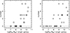 |
Fig. 17. Number of additional galaxies in a 1.5° × 1.5° area around the target galaxies, within a velocity range of −500 to +500 km s−1 with respect to the central velocity of the target galaxy. This number is plotted against the H I mass of the target galaxy in the left panel and against the stellar mass in the right panel. Note the sudden increase at MH I ∼ 109 M⊙ (left) and M⋆ ∼ 108 M⊙ (right). |
We can compare this with a similar observational result found by Zhu & Putman (2023). In a census of gaseous satellites around spiral galaxies, they identify companion galaxies around local spiral galaxies identified in the ALFALFA survey, and find that the number starts to increase at a halo mass of log(Mhalo/M⊙)∼11.5. Using their Table 1 for a first-order conversion of their halo masses to H I masses, we find that this sudden increase occurs at an H I mass just below 109 M⊙, strikingly close to where we find an increase in our sample.
Applying a more restrictive definition of a companion galaxy, analogous to that used in Zhu & Putman (2023), does not substantially change our results. For example, imposing a cut of ±300 km s−1 with respect to the systemic velocity, and a cut in projected separation to the companion of 200 kpc (the approximate value of the virial radius R200 for the upper mass range of the sample) does not change the observed sudden increase.
It is interesting to note that that many of these gas-rich companion galaxies are found projected within the virial radius, contrary to what we see in the Local Group (Spekkens et al. 2014), but consistent with recent SAGA results (Mao et al. 2021) with many star forming galaxies projected within the virial radii.
A more complete census of the companion galaxy population will be possible when the full-depth data for the full sample are available and we can probe the companion population to the fullest extent possible for our survey. As with the galaxies presented here, these satellites and companions will be resolved spatially and spectrally, meaning that in-depth studies of the dark matter content and baryon fractions can be made down to an H I mass limit of ∼106 M⊙ (cf. Table 4), a regime previously only accessible in the Local Group. A first discovery of such a low-mass galaxy in the MHONGOOSE observations is presented in Maccagni et al. (2024).
9. Summary
We present a description of the MHONGOOSE survey, a large, deep, high-resolution H I survey on MeerKAT of 30 nearby gas-rich spiral and dwarf galaxies. The total survey comprises 1650h of observing time, with 55h allocated per galaxy. The main science goal of MHONGOOSE is to characterize the low-column density H I in these galaxies, linking it with various cold-gas-accretion scenarios. Other science goals include detailed explorations of the link between H I and star formation, and the kinematics of the galaxies, constraints on the presence and distribution of dark matter, as well as the environments of the targets. The sample covers approximately three orders of magnitude in H I mass, from low-mass MH I ∼ 107 M⊙ as typically found in dwarf galaxies to MH I ∼ 1010 M⊙ as found in large spiral galaxies. In this paper, we present the survey, the sample, and a summary of the observations. In addition we describe the data reduction procedure and data products.
Each galaxy will eventually be observed for 55h in ten tracks of 5.5h each, and we produce full-depth data cubes at a velocity resolution of 1.4 km s−1 and a range in angular resolutions from ∼8″ as the highest resolution to ∼90″ as our lowest resolution. The resulting column density sensitivity (3σ over 16 km s−1) ranges from 4.3 × 1019 cm−2 at the highest resolution to 4.2 × 1017 cm−2 at the lowest resolution. The 3σ and 50 km s−1 mass-detection limit is 5.4 × 10⁵ M⊙ at 10 Mpc, which is the median distance of the sample.
We present first results based on the full-depth data of a limited number of galaxies and single-track observations of the complete sample (with the latter observations comprising 10% of the survey data). Comparing full-depth, single-track, and single-dish data, we show that MeerKAT is excellent at recovering the total fluxes of our sample galaxies. We also show that the full-depth data detect on average ∼2% more H I than the single-track data. While this increase may seem modest, the additional H I mass it represents is sufficient to allow the existence of a ∼1018 cm−2 low-column-density H I component in the disks of our galaxies. This demonstrates the difficulty in investigating the presence of low-column-density H I using total H I mass measurements.
We also investigated the link between the local H I surface density and the velocity “dispersion” in all of our sample galaxies. We recover the well-known upper limit on H I surface density (measured on kpc scales), and find a lower limit to the measured second-moment value of ∼8.5 km s−1. We find that the H I surface density has two distinct locations in a surface density–velocity dispersion diagram: one at ∼5 × 1020 cm−2, representing the gas in the star-forming disks, and one at ∼5 × 1019 cm−2 representing gas not participating in star formation. The two regions are distinct and separated at an H I surface density of 2 × 1020 cm−2. Previous studies (e.g., Kanekar et al. 2011) showed that, at this surface density, a rapid change in spin temperature occurs, and that this is the column density where the formation of a cool and dense component of the ISM starts.
We give an overview of all additional galaxies detected in the single-track data. These are defined as the sources detected in H I that were not targeted by the survey but were nevertheless found within the 1.5 ° ×1.5° area and spanning 1000 km s−1 in velocity range around the target galaxies. We find that half of these 49 galaxies have cataloged optical counterparts that coincide in position and velocity. Just under half have cataloged optical counterparts that coincide in position but that had until now no previously measured redshifts. Five of our additional galaxies have optical counterparts that have not been previously cataloged. We have not found any H I detections that do not have optical counterparts.
Studies of the full-depth data will be presented in future papers. However, based on the results shown here, it is already clear that the MHONGOOSE data are of excellent quality, showing great promise for future work on the low-column-density H I in nearby galaxies.
CARACal and its related software packages can be found in the repository collection at https://github.com/caracal-pipeline/
We note that here we adopt the informal definition that the second moment is equal to the dispersion. Mathematically, the second moment is defined as the variance.
The color map used for the velocity field is based on the perception-based color maps available as part of the CosmosCanvas project: https://ascl.net/code/v/3580
Acknowledgments
It is a pleasure to thank SARAO staff past and present for their help in making MHONGOOSE a reality. The MeerKAT telescope is operated by the South African Radio Astronomy Observatory, which is a facility of the National Research Foundation, an agency of the Department of Science and Innovation. This work has received funding from the European Research Council (ERC) under the European Union’s Horizon 2020 research and innovation programme (grant agreement No. 882793 “MeerGas”). We thank SURF, and particularly Dr. Raymond Oonk for the support in the early stages of the data reduction. KAO is supported by a Royal Society Dorothy Hodgkin Fellowship, by STFC through grant ST/T000244/1, and by the European Research Council (ERC) through Advanced Investigator grant to C.S. Frenk, DMIDAS (GA 786910). DJP, NZ and SK are supported through the South African Research Chairs Initiative of the Department of Science and Technology and National Research Foundation (Grant number 77825). EA and AB thank the CNES for financial support. LC acknowledges funding from the Chilean Agencia Nacional de Investigación y Desarrollo (ANID) through Fondo Nacional de Desarrollo Científico y Tecnológico (FONDECYT) Regular Project 1210992. The work at AIRUB is supported by the German Federal Ministry of Education and Research (BMBF) Verbundforschung grant 05A20PC4 (Verbundprojekt D-MeerKAT-II). KS acknowledges support from the Natural Sciences and Engineering Research Council of Canada (NSERC). LVM and AS acknowledge financial support from the grant CEX2021-001131-S funded by MCIN/AEI/10.13039/501100011033 and from the grant PID2021-123930OB-C21 funded by MCIN/AEI/10.13039/501100011033, by “ERDF A way of making Europe” and by the European Union. BN acknowledges financial support from the Severo Ochoa grant CEX2021-001131-S funded by MCIN/AEI/10.13039/501100011033. This research has made use of the NASA/IPAC Extragalactic Database (NED), which is funded by the National Aeronautics and Space Administration and operated by the California Institute of Technology. This research has made use of the SIMBAD database, operated at CDS, Strasbourg, France. The Legacy Surveys consist of three individual and complementary projects: the Dark Energy Camera Legacy Survey (DECaLS; Proposal ID #2014B-0404; PIs: David Schlegel and Arjun Dey), the Beijing-Arizona Sky Survey (BASS; NOAO Prop. ID #2015A-0801; PIs: Zhou Xu and Xiaohui Fan), and the Mayall z-band Legacy Survey (MzLS; Prop. ID #2016A-0453; PI: Arjun Dey). DECaLS, BASS and MzLS together include data obtained, respectively, at the Blanco telescope, Cerro Tololo Inter-American Observatory, NSF’s NOIRLab; the Bok telescope, Steward Observatory, University of Arizona; and the Mayall telescope, Kitt Peak National Observatory, NOIRLab. Pipeline processing and analyses of the data were supported by NOIRLab and the Lawrence Berkeley National Laboratory (LBNL). The Legacy Surveys project is honored to be permitted to conduct astronomical research on Iolkam Du’ag (Kitt Peak), a mountain with particular significance to the Tohono O’odham Nation. NOIRLab is operated by the Association of Universities for Research in Astronomy (AURA) under a cooperative agreement with the National Science Foundation. LBNL is managed by the Regents of the University of California under contract to the U.S. Department of Energy. This project used data obtained with the Dark Energy Camera (DECam), which was constructed by the Dark Energy Survey (DES) collaboration. Funding for the DES Projects has been provided by the U.S. Department of Energy, the U.S. National Science Foundation, the Ministry of Science and Education of Spain, the Science and Technology Facilities Council of the United Kingdom, the Higher Education Funding Council for England, the National Center for Supercomputing Applications at the University of Illinois at Urbana-Champaign, the Kavli Institute of Cosmological Physics at the University of Chicago, Center for Cosmology and Astro-Particle Physics at the Ohio State University, the Mitchell Institute for Fundamental Physics and Astronomy at Texas A&M University, Financiadora de Estudos e Projetos, Fundacao Carlos Chagas Filho de Amparo, Financiadora de Estudos e Projetos, Fundacao Carlos Chagas Filho de Amparo a Pesquisa do Estado do Rio de Janeiro, Conselho Nacional de Desenvolvimento Cientifico e Tecnologico and the Ministerio da Ciencia, Tecnologia e Inovacao, the Deutsche Forschungsgemeinschaft and the Collaborating Institutions in the Dark Energy Survey. The Collaborating Institutions are Argonne National Laboratory, the University of California at Santa Cruz, the University of Cambridge, Centro de Investigaciones Energeticas, Medioambientales y Tecnologicas-Madrid, the University of Chicago, University College London, the DES-Brazil Consortium, the University of Edinburgh, the Eidgenossische Technische Hochschule (ETH) Zurich, Fermi National Accelerator Laboratory, the University of Illinois at Urbana-Champaign, the Institut de Ciencies de l’Espai (IEEC/CSIC), the Institut de Fisica d’Altes Energies, Lawrence Berkeley National Laboratory, the Ludwig Maximilians Universitat Munchen and the associated Excellence Cluster Universe, the University of Michigan, NSF’s NOIRLab, the University of Nottingham, the Ohio State University, the University of Pennsylvania, the University of Portsmouth, SLAC National Accelerator Laboratory, Stanford University, the University of Sussex, and Texas A&M University. BASS is a key project of the Telescope Access Program (TAP), which has been funded by the National Astronomical Observatories of China, the Chinese Academy of Sciences (the Strategic Priority Research Program “The Emergence of Cosmological Structures” Grant # XDB09000000), and the Special Fund for Astronomy from the Ministry of Finance. The BASS is also supported by the External Cooperation Program of Chinese Academy of Sciences (Grant # 114A11KYSB20160057), and Chinese National Natural Science Foundation (Grant # 12120101003, # 11433005). The Legacy Survey team makes use of data products from the Near-Earth Object Wide-field Infrared Survey Explorer (NEOWISE), which is a project of the Jet Propulsion Laboratory/California Institute of Technology. NEOWISE is funded by the National Aeronautics and Space Administration. The Legacy Surveys imaging of the DESI footprint is supported by the Director, Office of Science, Office of High Energy Physics of the U.S. Department of Energy under Contract No. DE-AC02-05CH1123, by the National Energy Research Scientific Computing Center, a DOE Office of Science User Facility under the same contract; and by the U.S. National Science Foundation, Division of Astronomical Sciences under Contract No. AST-0950945 to NOAO. Data availability: The single-track moment maps presented in this paper are available for download at the MHONGOOSE website (https://mhongoose.astron.nl) or through a DOI (https://zenodo.org/doi/10.5281/zenodo.10907079).
References
- Anand, G. S., Lee, J. C., Van Dyk, S. D., et al. 2021, MNRAS, 501, 3621 [Google Scholar]
- Auld, R., Minchin, R. F., Davies, J. I., et al. 2006, MNRAS, 371, 1617 [NASA ADS] [CrossRef] [Google Scholar]
- Barnes, D. G., Staveley-Smith, L., de Blok, W. J. G., et al. 2001, MNRAS, 322, 486 [Google Scholar]
- Bigiel, F., Leroy, A., Walter, F., et al. 2008, AJ, 136, 2846 [NASA ADS] [CrossRef] [Google Scholar]
- Bigiel, F., Leroy, A., Walter, F., et al. 2010, AJ, 140, 1194 [NASA ADS] [CrossRef] [Google Scholar]
- Bigiel, F., Leroy, A. K., Walter, F., et al. 2011, ApJ, 730, L13 [NASA ADS] [CrossRef] [Google Scholar]
- Braun, R. 1997, ApJ, 484, 637 [NASA ADS] [CrossRef] [Google Scholar]
- Braun, R., & Thilker, D. A. 2004, A&A, 417, 421 [NASA ADS] [CrossRef] [EDP Sciences] [Google Scholar]
- Camilo, F. 2018, Nat. Astron., 2, 594 [CrossRef] [Google Scholar]
- Crain, R. A., Bahé, Y. M., Lagos, C. d. P., et al. 2016, MNRAS, 464, 4204 [Google Scholar]
- Davé, R., Hernquist, L., Katz, N., & Weinberg, D. H. 1999, ApJ, 511, 521 [Google Scholar]
- de Blok, W. J. G., Keating, K. M., Pisano, D. J., et al. 2014, A&A, 569, A68 [NASA ADS] [CrossRef] [EDP Sciences] [Google Scholar]
- de Blok, W. J. G., Adams, E. A. K., Amram, P., et al. 2016, Proceedings of MeerKAT Science: On the Pathway to the SKA -PoS(MeerKAT2016), 007 [Google Scholar]
- de Blok, W. J. G., Walter, F., Ferguson, A. M. N., et al. 2018, ApJ, 865, 26 [NASA ADS] [CrossRef] [Google Scholar]
- de Blok, W. J. G., Athanassoula, E., Bosma, A., et al. 2020, A&A, 643, A147 [NASA ADS] [CrossRef] [EDP Sciences] [Google Scholar]
- Dey, A., Schlegel, D. J., Lang, D., et al. 2019, AJ, 157, 168 [Google Scholar]
- Di Teodoro, E. M., & Fraternali, F. 2014, A&A, 567, A68 [NASA ADS] [CrossRef] [EDP Sciences] [Google Scholar]
- Di Teodoro, E. M., & Fraternali, F. 2015, MNRAS, 451, 3021 [Google Scholar]
- Elagali, A., Staveley-Smith, L., Rhee, J., et al. 2019, MNRAS, 487, 2797 [NASA ADS] [CrossRef] [Google Scholar]
- Espada, D., Muñoz-Mateos, J. C., Gil de Paz, A., et al. 2011a, ApJ, 736, 20 [NASA ADS] [CrossRef] [Google Scholar]
- Espada, D., Verdes-Montenegro, L., Huchtmeier, W. K., et al. 2011b, A&A, 532, A117 [NASA ADS] [CrossRef] [EDP Sciences] [Google Scholar]
- Fraternali, F. 2017, Astrophys. Space Sci. Lib., 430, 323 [CrossRef] [Google Scholar]
- Fraternali, F., & Tomassetti, M. 2012, MNRAS, 426, 2166 [NASA ADS] [CrossRef] [Google Scholar]
- Fraternali, F., Oosterloo, T., Sancisi, R., & Moorsel, G. V. 2001, ApJ, 562, L47 [CrossRef] [Google Scholar]
- Haynes, M. P., Giovanelli, R., Kent, B. R., et al. 2018, ApJ, 861, 49 [Google Scholar]
- Heald, G., Józsa, G., Serra, P., et al. 2011, A&A, 526, A118 [NASA ADS] [CrossRef] [EDP Sciences] [Google Scholar]
- Heald, G., de Blok, W. J. G., Lucero, D., et al. 2016, MNRAS, 462, 1238 [NASA ADS] [CrossRef] [Google Scholar]
- Healy, J., de Blok, W.J.G., Maccagni, F.M., et al. 2024, A&A, 687, A254 [NASA ADS] [CrossRef] [EDP Sciences] [Google Scholar]
- Hess, K. M., Jarrett, T. H., Carignan, C., Passmoor, S. S., & Goedhart, S. 2015, MNRAS, 452, 1617 [Google Scholar]
- Hunter, D. A., Ficut-Vicas, D., Ashley, T., et al. 2012, AJ, 144, 134 [CrossRef] [Google Scholar]
- Ianjamasimanana, R., de Blok, W. J. G., & Heald, G. H. 2017, AJ, 153, 213 [NASA ADS] [CrossRef] [Google Scholar]
- Irwin, J. A., Hoffman, G. L., Spekkens, K., et al. 2009, ApJ, 692, 1447 [NASA ADS] [CrossRef] [Google Scholar]
- Jarrett, T. H., Cluver, M. E., Taylor, E. N., et al. 2023, ApJ, 946, 95 [NASA ADS] [CrossRef] [Google Scholar]
- Jonas, J. 2018, Proceedings of MeerKAT Science: On the Pathway tothe SKA - PoS(MeerKAT2016), 001 [Google Scholar]
- Jones, M. G., Espada, D., Verdes-Montenegro, L., et al. 2017, A&A, 609, A17 [Google Scholar]
- Józsa, G. I., Andati, L. A., de Blok, W., et al. 2020, ASP Conf. Ser., 532, 447 [Google Scholar]
- Kamphuis, P., Jütte, E., Heald, G. H., et al. 2022, A&A, 668, A182 [NASA ADS] [CrossRef] [EDP Sciences] [Google Scholar]
- Kanekar, N., Braun, R., & Roy, N. 2011, ApJ, 737, L33 [NASA ADS] [CrossRef] [Google Scholar]
- Karachentsev, I. D., Sharina, M. E., Dolphin, A. E., et al. 2002, A&A, 385, 21 [CrossRef] [EDP Sciences] [Google Scholar]
- Kennicutt, R. C. 1998, ApJ, 498, 541 [NASA ADS] [CrossRef] [Google Scholar]
- Kere\u{s}, D., Katz, N., Weinberg, D. H., & Davé, R. 2005, MNRAS, 363, 2 [CrossRef] [Google Scholar]
- Koribalski, B. S., Staveley-Smith, L., Kilborn, V. A., et al. 2004, AJ, 128, 16 [Google Scholar]
- Koribalski, B. S., Wang, J., Kamphuis, P., et al. 2018, MNRAS, 478, 1611 [NASA ADS] [CrossRef] [Google Scholar]
- Koribalski, B. S., Staveley-Smith, L., Westmeier, T., et al. 2020, Ap&SS, 365, 118 [Google Scholar]
- Kourkchi, E., & Tully, R. B. 2017, ApJ, 843, 16 [NASA ADS] [CrossRef] [Google Scholar]
- Kregel, M., Kruit, P. C. V. D., & de Blok, W. J. G. 2004, MNRAS, 352, 768 [NASA ADS] [CrossRef] [Google Scholar]
- Krumholz, M. R., McKee, C. F., & Tumlinson, J. 2009, ApJ, 693, 216 [NASA ADS] [CrossRef] [Google Scholar]
- Leon, S., Verdes-Montenegro, L., Sabater, J., et al. 2008, A&A, 485, 475 [NASA ADS] [CrossRef] [EDP Sciences] [Google Scholar]
- Leroy, A. K., Walter, F., Brinks, E., et al. 2008, AJ, 136, 2782 [Google Scholar]
- Leroy, A. K., Walter, F., Sandstrom, K., et al. 2013, AJ, 146, 19 [Google Scholar]
- Leroy, A. K., Sandstrom, K. M., Lang, D., et al. 2019, ApJS, 244, 24 [Google Scholar]
- Lisenfeld, U., Verdes-Montenegro, L., Sulentic, J., et al. 2007, A&A, 462, 507 [NASA ADS] [CrossRef] [EDP Sciences] [Google Scholar]
- Liu, Y., Zhu, M., Yu, H., et al. 2023, MNRAS, 523, 3905 [NASA ADS] [CrossRef] [Google Scholar]
- Lucero, D. M., Carignan, C., Elson, E. C., et al. 2015, MNRAS, 450, 3935 [NASA ADS] [CrossRef] [Google Scholar]
- Maccagni, F. M., Morganti, R., Oosterloo, T. A., Geréb, K., & Maddox, N. 2017, A&A, 604, A43 [NASA ADS] [CrossRef] [EDP Sciences] [Google Scholar]
- Maccagni, F. M., Serra, P., Gaspari, M., et al. 2021, A&A, 656, A45 [NASA ADS] [CrossRef] [EDP Sciences] [Google Scholar]
- Maccagni, F. M., Healy, J., de Blok, W. J. G., & Serra, P. 2022, MeerKAT Technical Report, http://dx.doi.org/10.48479/bhpj-nz95 [Google Scholar]
- Maccagni, F. M., de Blok, W. J. G., Mancera Piña, P. E., et al. 2024, A&A, in press https://doi.org/10.1051/0004-6361/202449441 [Google Scholar]
- Makhathini, S. 2018, PhD Thesis, Rhodes University, South Africa [Google Scholar]
- Mao, Y.-Y., Geha, M., Wechsler, R. H., et al. 2021, ApJ, 907, 85 [NASA ADS] [CrossRef] [Google Scholar]
- Marasco, A., Fraternali, F., & Binney, J. J. 2012, MNRAS, 419, 1107 [NASA ADS] [CrossRef] [Google Scholar]
- Marasco, A., Fraternali, F., Heald, G., et al. 2019, A&A, 631, A50 [NASA ADS] [CrossRef] [EDP Sciences] [Google Scholar]
- Mauch, T., Cotton, W. D., Condon, J. J., et al. 2020, ApJ, 888, 61 [Google Scholar]
- McKee, C. F., & Krumholz, M. R. 2010, ApJ, 709, 308 [NASA ADS] [CrossRef] [Google Scholar]
- Meurer, G. R., Staveley-Smith, L., & Killeen, N. E. B. 1998, MNRAS, 300, 705 [CrossRef] [Google Scholar]
- Meurer, G. R., Hanish, D. J., Ferguson, H. C., et al. 2006, ApJS, 165, 307 [NASA ADS] [CrossRef] [Google Scholar]
- Meurer, G. R., Zheng, Z., & de Blok, W. J. G. 2013, MNRAS, 429, 2537 [NASA ADS] [CrossRef] [Google Scholar]
- Meyer, M. J., Zwaan, M. A., Webster, R. L., et al. 2004, MNRAS, 350, 1195 [Google Scholar]
- Moster, B. P., Naab, T., & White, S. D. M. 2013, MNRAS, 428, 3121 [Google Scholar]
- Offringa, A. R., McKinley, B., Hurley-Walker, N., et al. 2014, MNRAS, 444, 606 [Google Scholar]
- Oosterloo, T., Fraternali, F., & Sancisi, R. 2007, AJ, 134, 1019 [Google Scholar]
- Pingel, N. M., Pisano, D. J., Heald, G., et al. 2018, ApJ, 865, 36 [NASA ADS] [CrossRef] [Google Scholar]
- Pisano, D. J. 2014, AJ, 147, 48 [NASA ADS] [CrossRef] [Google Scholar]
- Popping, A., Davé, R., Braun, R., & Oppenheimer, B. D. 2009, A&A, 504, 15 [NASA ADS] [CrossRef] [EDP Sciences] [Google Scholar]
- Pritzl, B. J., Knezek, P. M. III, John, S. G., et al. 2003, ApJ, 596, L47 [CrossRef] [Google Scholar]
- Putman, M., Peek, J., & Joung, M. 2012, ARA&A, 50, 491 [NASA ADS] [CrossRef] [Google Scholar]
- Ramesh, R., Nelson, D., & Pillepich, A. 2023, MNRAS, 518, 5754 [Google Scholar]
- Sabater, J., Verdes-Montenegro, L., Leon, S., Best, P., & Sulentic, J. 2012, A&A, 545, A15 [NASA ADS] [CrossRef] [EDP Sciences] [Google Scholar]
- Saintonge, A., Lutz, D., Genzel, R., et al. 2013, ApJ, 778, 2 [Google Scholar]
- Sancisi, R., Fraternali, F., Oosterloo, T., & van der Hulst, T. 2008, A&A Rev., 15, 189 [CrossRef] [Google Scholar]
- Sardone, A., Pisano, D. J., Pingel, N. M., et al. 2021, ApJ, 910, 69 [NASA ADS] [CrossRef] [Google Scholar]
- Schruba, A., Leroy, A. K., Kruijssen, J. M. D., et al. 2017, ApJ, 835, 278 [NASA ADS] [CrossRef] [Google Scholar]
- Serra, P., Oosterloo, T., Morganti, R., et al. 2012, MNRAS, 422, 1835 [Google Scholar]
- Serra, P., Westmeier, T., Giese, N., et al. 2015, MNRAS, 448, 1922 [Google Scholar]
- Serra, P., Maccagni, F. M., Kleiner, D., et al. 2023, A&A, 673, A146 [NASA ADS] [CrossRef] [EDP Sciences] [Google Scholar]
- Shapiro, P. R., & Field, G. B. 1976, ApJ, 205, 762 [NASA ADS] [CrossRef] [Google Scholar]
- Sorgho, A., Carignan, C., Pisano, D. J., et al. 2018, MNRAS, 482, 1248 [Google Scholar]
- Spekkens, K., Urbancic, N., Mason, B. S., Willman, B., & Aguirre, J. E. 2014, ApJ, 795, L5 [NASA ADS] [CrossRef] [Google Scholar]
- Sternberg, A., Petit, F. L., Roueff, E., & Bourlot, J. L. 2014, ApJ, 790, 10 [CrossRef] [Google Scholar]
- Sun, J., Leroy, A. K., Schruba, A., et al. 2018, ApJ, 860, 172 [NASA ADS] [CrossRef] [Google Scholar]
- Sun, J., Leroy, A. K., Schinnerer, E., et al. 2020, ApJ, 901, L8 [NASA ADS] [CrossRef] [Google Scholar]
- Tacconi, L. J., Genzel, R., Saintonge, A., et al. 2018, ApJ, 853, 179 [Google Scholar]
- Tully, R., & Fisher, J. 1977, A&A, 54, 661 [NASA ADS] [Google Scholar]
- Tully, R. B., Courtois, H. M., Dolphin, A. E., et al. 2013, AJ, 146, 86 [NASA ADS] [CrossRef] [Google Scholar]
- Tully, R. B., Courtois, H. M., & Sorce, J. G. 2016, AJ, 152, 50 [Google Scholar]
- Tumlinson, J., Peeples, M. S., & Werk, J. K. 2017, ARA&A, 55, 1 [Google Scholar]
- van der Hulst, J. M., van Albada, T. S., & Sancisi, R. 2001, ASP Conf. Proc., 240, 451 [NASA ADS] [Google Scholar]
- Verheijen, M. A. W., & Sancisi, R. 2001, A&A, 370, 765 [NASA ADS] [CrossRef] [EDP Sciences] [Google Scholar]
- Veronese, S., de Blok, W. J. G., & Walter, F. 2023, A&A, 672, A55 [NASA ADS] [CrossRef] [EDP Sciences] [Google Scholar]
- Wakker, B. P., & Woerden, H. V. 1997, ARA&A, 35, 217 [NASA ADS] [CrossRef] [Google Scholar]
- Walter, F., Brinks, E., de Blok, W. J. G., et al. 2008, AJ, 136, 2563 [Google Scholar]
- Walter, F., Carilli, C., Neeleman, M., et al. 2020, ApJ, 902, 111 [Google Scholar]
- Westmeier, T., Kitaeff, S., Pallot, D., et al. 2021, MNRAS, 506, 3962 [NASA ADS] [CrossRef] [Google Scholar]
- Wolfe, S. A., Pisano, D. J., Lockman, F. J., McGaugh, S. S., & Shaya, E. J. 2013, Nature, 497, 224 [NASA ADS] [CrossRef] [Google Scholar]
- Wolfe, S. A., Lockman, F. J., & Pisano, D. J. 2016, ApJ, 816, 81 [NASA ADS] [CrossRef] [Google Scholar]
- Wolfire, M. G., McKee, C. F., Hollenbach, D., & Tielens, A. G. G. M. 2003, ApJ, 587, 278 [Google Scholar]
- Wong, T., & Blitz, L. 2002, ApJ, 569, 157 [CrossRef] [Google Scholar]
- Wong, O. I., Meurer, G. R., Zheng, Z., et al. 2016, MNRAS, 460, 1106 [NASA ADS] [CrossRef] [Google Scholar]
- Xu, C. K., Cheng, C., Appleton, P. N., et al. 2022, Nature, 610, 461 [NASA ADS] [CrossRef] [Google Scholar]
- Zhu, J., & Putman, M. E. 2023, MNRAS, 521, 3765 [NASA ADS] [CrossRef] [Google Scholar]
Appendix A: Atlas of single-track moment maps
In Fig. A.1 we show the r05_t00 single-track moment maps of the entire sample. A short description of the panels that are shown (from left to right) for each galaxy follows.
The left-most panel shows a combined optical grz color image from DECaLS DR9 (except for J1303–17b where we use a giz image from DR10). The next panel shows the zeroth-moment or integrated H I map. The lowest column density contour shown corresponds to a S/N of 3 (see Sect. 5.9 for a description). This value is listed at the bottom of the zeroth-moment panel. Subsequent contours then increase by a factor 2n, where n = 0, 2, 4, ....
In the third panel we show the first-moment map or intensity-weighted velocity field. Here we indicate the central velocity (as listed in Table 1) with a thick contour. The central velocity is defined from the integrated H I profile as the velocity halfway between the velocities where the flux density equals 20% of the peak value (see Sect. 6.2). Other contours are spaced by 10 or 20 km s−1 with respect to this velocity, as listed in the panel. The color map indicates whether velocities are receding (red) or approaching (blue).
The second-moment maps are shown using the same intensity scale for all galaxies. For all galaxies, the color map shows the same velocity range from 0 (light-blue) to 30 (red) km s−1. Contours start at 12 km s−1, and increase in steps of 12 km s−1. For reference, the 24 km s−1 contour is shown in black. Both the first- and second-moment maps have been masked such that only values with S/N > 3 in the zeroth-moment map are shown. While we do not present a full analysis of the first- and second-moment maps in this paper, we do caution that for the edge-on galaxies, these have to be interpreted with care because of the strong projection effects.
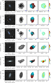 |
Fig. A.1. Single-track moment maps for the MHONGOOSE galaxies using the r05_t00 resolution. From left to right: (i): Combined grz-color image from DECaLS. (ii): primary-beam corrected zeroth-moment or integrated H I intensity map. Contours as indicated in the Figure. The lowest contour represents S/N = 3, with subsequent contour levels increasing by factors of two. (iii): First-moment map or intensity-weighted velocity field. Red colors indicate the receding side, blue colors the approaching side. The central velocity (listed in Tab. 1) is indicated by the thick contour. Other contours are spaced by 10 or 20 km s−1, as indicated in the Figure. (iv): Second-moment map: the colors show the range from 0 (light-blue) to 30 (red) km s−1. The lowest contour shows the 12 km s−1 level, and subsequent contours are spaced by 12 km s−1. The 24 km s−1 contour is shown in black. See text for a more extensive description. |
-1
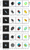 |
Fig. A.2. Single-track moment maps of MHONGOOSE galaxies. |
-1
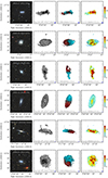 |
Fig. A.3. Single-track moment maps of MHONGOOSE galaxies. |
-1
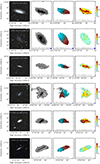 |
Fig. A.4. Single-track moment maps of MHONGOOSE galaxies. |
-1
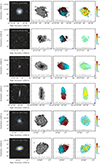 |
Fig. A.5. Single-track moment maps of MHONGOOSE galaxies. |
Appendix B: The effect of beam smearing and inclination on second-moment values
The column density-second moment distributions shown in Figs. 12 and 13 were derived using the r15_t00 standard resolution with a beam size of ∼30″. This beam size, in combination with the angular sizes of the galaxies, could potentially lead to inflated second-moment values due to beam smearing (especially in the centers of the galaxies). In addition, long line-of-sight effects in the high-inclination galaxies could also contribute to higher second-moment values. Here we address these potential issues and show that they do not significantly affect the distribution shown in Fig. 13.
We test the effect of beam smearing by creating a model galaxy similar to one of our sample galaxies, convolving it to the observed resolution and inserting it in a data cube with a noise level equal to that found for the observations. We then treat it exactly as the sample galaxies for the derivation of the moment maps and creation of the moment distributions.
We use as the basis of our model the rotation curve and H I radial profile of NGC1566 as presented in Elagali et al. (2019). We approximate the rotation curve with a linear, steep rise from 0 to 180 km s−1 in the inner 5 kpc. At larger radii we assume a constant rotation velocity of 180 km s−1 (cf. Fig. 10 in Elagali et al. 2019). For the H I distribution we assume a central value of log(NH I/M⊙ pc−2) = 1, with log(NH I) linearly decreasing with radius until log(NH I/M⊙ pc−2) = −0.5 at 50 kpc (cf. Fig. 12 in Elagali et al. 2019). For the purposes of this exercise we extend the radial range of the model to 100 kpc by assuming that the rotation curve stays flat, and that the log(NH I) values keep decreasing at the same rate as inside 50 kpc. We adopt a value of 30 degrees for the inclination (cf. Fig 10 in Elagali et al. 2019). For the velocity dispersion of the H I we use a constant value of 10 km s−1. The H I disk is assumed to be thin, with a scale height of 100 pc. We assume the same distance and systemic velocity as for the real NGC 1566 (17.6 Mpc and 1496 km s−1, respectively; cf. Tab. 1). With these parameters we create a model cube using the GALMOD section of the 3DBAROLO software package (Di Teodoro & Fraternali 2015) with a beam size equal to that of the r15_t00 standard resolution. We insert this model in a cube filled with an rms noise of 0.48 mJy (again at the r15_t00 resolution), consistent with the noise values typically found in the single-track cubes.
Zeroth- and second-moment maps of the model are then created with SoFiA-2 in an identical manner as for the real galaxies. We plot the resulting column density-second moment distribution in Fig. B.1 (right panel), comparing it with the observed NGC 1566 distribution (left panel). Several noteworthy features can be seen. Firstly, in the model we see a plume towards high second-moment values at the highest column densities. This is caused by beam smearing due to the slope of the inner rotation curve. Secondly, on the low-column density end of the distribution we see the familiar tail towards low second-moment value due to masking (as discussed in Sect. 7.3). Finally, in the intermediate column density range, we see the constant second-moment values. The limited resolution has slightly increased the average value from its original 10 km s−1, but only by ∼1 km s−1 or less. These therefore are a good reflection of the velocity dispersion in the model disk.
In summary, only the high second-moment values at the highest column densities (corresponding to the innermost part of the disk where the rotation curve rises) can be attributed to beam smearing. Higher second-moment values at lower column densities (i.e., further out in the disk) reflect higher velocity dispersions, or the presence of multiple components along the line of sight.
We can compare the distribution shown in Fig. B.1 (right panel) with the more complex distribution for the real NGC 1566 in Fig. B.1 (left panel). The latter shows higher second-moment values over a larger range in column densities, indicating that a significant fraction of these higher values are not due to beam smearing. Inspection of Fig. 12 shows that these are caused by high-second moment components in galaxies with overall low second-moment values (e.g., J0419–54) as well as galaxies that have overall higher second-moment values (e.g., J1318–21).
We can test this further by taking the inclinations of the galaxies into account. In general, the broadening of profiles due to beam smearing and length of the line of sight through the disk increases dramatically towards high inclinations, with the effect strongest in edge-on galaxies. There is therefore a possibility that high-inclination galaxies contribute to the higher second-moment values we observe at intermediate column densities (i.e., around ∼1020 cm−2). In Fig. B.2 (left panel) we show the distribution from Fig. 13, which includes all galaxies in the sample, at all inclinations, including edge-ons. To remove the effect that high-inclination galaxies may have on the distribution, we show in the centre panel the distribution of galaxies with an inclination i < 60° (16 galaxies) and in the right panel the distribution with i < 70° (22 galaxies). Comparison of these distributions shows that omitting the high-inclination galaxies mainly affects the width of the second-moment distribution in the low-column density tail. The effects in the intermediate and high-column density ranges are much less pronounced, and the distribution remains essentially the same in these column density regimes.
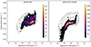 |
Fig. B.1. Comparison of the column density-second moment distribution of a model galaxy built to resemble NGC 1566 with that of NGC 1566 itself. The observed distribution is shown in the left panel; the model in the right panel. For the model we use a single, thin H I disk with a velocity dispersion of 10 km s−1. The model galaxy is “observed” and treated just like the single-track MHONGOOSE galaxies. Note the plume due to beam smearing at the high column density end, and the masking tail at the low column density end. The model does not show the high second-moment values at intermediate column densities that are present in the observations. |
 |
Fig. B.2. Comparison of the column density-second moment distribution for a number of inclination limits. The left panel shows the distribution as shown in Fig. 13 without any inclination limits. The centre panel shows the distribution when limited to galaxies with inclination i < 60°. The right panel shows the same for i < 70°. |
All Tables
All Figures
|
Fig. 1. Noise level as a function of resolution for the HALOGAS, THINGS, and MHONGOOSE surveys. The blue curve shows that the MHONGOOSE survey has a flat noise distribution, meaning equally sensitive imaging can be obtained over a large range of resolutions between ∼6″ and ∼90″. The dashed brown curve shows the HALOGAS survey, with an optimal sensitivity at around ∼20″. The dashed red curve represents the THINGS survey. This is a combination of three separate VLA array configurations (also shown at the top of the plot calculated using the correct relative observing times). THINGS has optimal sensitivity at around ∼15″ and ∼50″. All noise values are calculated over a 5 km s−1 channel. |
| In the text | |
|
Fig. 2. Sensitivity versus resolution in H I surveys. Colored symbols show the 3σ column density sensitivity over 16 km s−1 for various interferometric and single-dish surveys, as indicated by the labels and legend and listed in the text. The thick blue line shows the observed MHONGOOSE sensitivities. MHONGOOSE reaches single-dish sensitivities but at a 10–50 times better angular resolution. To give an indication of the physical scales: at 10.3 Mpc (the median distance of the MHONGOOSE sample), 10″ corresponds to 0.5 kpc. Galaxies that are part of a sample with a fixed angular resolution (THINGS 30″, GBT, and PKS) were given small, random horizontal offsets for clarity. References are given in the text. |
| In the text | |
|
Fig. 3. Star formation rates of the MHONGOOSE galaxies plotted against their stellar masses. Top panel: the SFR as derived using the method described in Cluver et al. (in prep.) based on mid-IR and UV SFRs. The stellar masses are derived from WISE W3 and W4 luminosities as described in Jarrett et al. (2023). Background grayscale and gray contours show the distribution of galaxies in the local Universe based on mid-IR and UV data (Jarrett & Cluver, in prep.). The MHONGOOSE sample was selected to be representative of the SFR–M⋆ main sequence (the upper ridge of the distributions) and almost all galaxies are indeed on this sequence. Only NGC 1371 (J0335–24) has a low SFR for its mass. Galaxies with uncertain SFR values are not plotted (see Table 1). UGCA320 (J1303–17b) has a low S/N in the WISE observations as indicated by the diamond symbol. The purple dashed curve shows the average trend derived in Cluver et al. (in prep.). Bottom panel: this shows the specific SFR of the MHONGOOSE galaxies plotted against stellar mass. Symbols and curves as in top panel. In addition, the blue curve shows a fit to the data presented in Leroy et al. (2019). The diagonal gray dashed lines indicate corresponding SFR values in M⊙ yr−1. |
| In the text | |
|
Fig. 4. Overview of the u = 0 flagging procedure. The top row shows a 100-channel binned empty map with horizontal stripes of one target scan of a NGC 1566 observation on the left, and on the right the corresponding FFT amplitude image, which shows a prominent vertical RFI feature at u = 0. The middle row shows the same plots, but after removal of the u = 0 stripe using our flagging procedure. The bottom row shows two zeroth-moment H I maps of NGC 1566, both created using a simple 2σ intensity cut. The bottom-left panel shows the map with the u = 0 RFI still included. The bottom-right panel shows the same map but with the u = 0 RFI removed. |
| In the text | |
|
Fig. 5. Sensitivities of the full-depth data cubes. The top panel shows the average noise per 1.4 km s−1 channel for the six standard resolutions, as averaged over full-depth observations of ten galaxies (cf. Fig. 1). Error bars show the rms difference in noise levels between the ten galaxies, but are generally comparable to or smaller than the symbol size. The bottom panel shows the 3σ, 16 km s−1 column density sensitivities. These are the same points as shown in Fig. 2. |
| In the text | |
|
Fig. 6. Natural-weighted noise values measured over a 1.4 km s−1 channel as a function of integration time for the observations of ESO 300-G014 (J0309–41). The black filled points indicate the measured noise level. The blue line shows the expected theoretical noise levels with a slope of −0.5. A linear fit to the observed noise levels gives a slope of −0.504. The red star indicates the target sensitivity from de Blok et al. (2016). |
| In the text | |
|
Fig. 7. Multi-resolution zeroth-moment maps of NGC 1566 (left panel) and NGC 5068 (right panel) based on the full-depth data. For each resolution, contours of 2n times the S/N = 3 value are shown (as listed in the legend). The resolutions shown are r05_t00 (red), r10_t00 (green), r15_t00 (blue), r05_t60 (purple), r10_t90 (olive). For each resolution two contours are shown, i.e., n = 0, 1, except for the highest resolution r05_t00 (red contour), where n = 0, 1, 2, … The r05_t00 moment map is shown in the background as a false color image, with the column density levels indicated by the color bar on the right. The beam sizes (colored according to the respective resolution) are shown in the bottom-right corner. |
| In the text | |
|
Fig. 8. Example single-track moment maps using the r05_t00 resolution for two MHONGOOSE galaxies. Top row: NGC 1566 (J0419–54); bottom row: NGC 5068 (J1318–21). From left to right: (i): Combined grz-color image from DECaLS. (ii): Primary-beam corrected zeroth-moment or integrated H I intensity map. Contours as indicated in the figure. The lowest contour represents S/N = 3, with subsequent contour levels increasing by a factor of two. (iii): First-moment map or intensity-weighted velocity field. Red colors indicate the receding side, blue colors the approaching side. The central velocity (listed in Table 1) is indicated by the thick contour. Other contours are spaced by 10 or 20 km s−1, as indicated in the Figure. (iv): Second-moment map: colors show the range from 0 (light-blue) to 30 (red) km s−1. The lowest contour shows the 12 km s−1 level, and subsequent contours are spaced by 12 km s−1. The 24 km s−1 contour is shown in black. For both the first- and second-moment maps, pixels corresponding to values below the S/N = 3 column density in the zeroth-moment map were blanked. See Appendix A for a more extensive description. |
| In the text | |
|
Fig. 9. Single-track (blue) and full-depth (orange) global H I profiles for ten of the MHONGOOSE galaxies as identified in the top left of each panel. The green arrows indicate the central velocities. We show only the velocity ranges where signal was present in the mask. |
| In the text | |
|
Fig. 10. Comparison of the MeerKAT and single-dish profiles. MeerKAT r15_t00 profiles are shown in black, GBT profiles (Sardone et al. 2021) in cyan, and HIPASS profiles (Koribalski et al. 2004) in red. The green arrows indicate the central velocties as derived from the MeerKAT data. |
| In the text | |
|
Fig. 11. Comparison of the single-track MeerKAT flux densities with single-dish flux densities. Stars (orange) indicate HIPASS values, filled circles (blue) GBT values. The full black line indicates a unity slope. The left panel compares the flux densities on a logarithmic scale, the right panel shows the same data points on a linear scale. The dashed blue line is a fit to the GBT points. The fit to the logarithmic GBT values has a slope of 0.968, the linear values give a fit with a slope of 0.954. The dotted orange line is a fit to the HIPASS data. Here the logarithmic slope is 0.964, the linear fit gives a slope of 0.860. |
| In the text | |
|
Fig. 12. Two-dimensional density histograms showing the distribution of inclination-corrected column densities and second moment values for the MHONGOOSE galaxies. Each histogram consists of 75 × 75 hexagonal bins, and only bins containing more than 4 pixels are shown. The color bar on the right in each panel indicates the number of pixels per bin. The background contours indicate the total distribution of the entire sample as shown in Fig. 13. Galaxies are divided in three bins in rotation velocity. Within each bin, galaxies are ordered by increasing inclination, with the most face-on galaxies in the top-left, and the most edge-on in the bottom-right. The two light-gray bars between the panels in each bin indicate inclinations of 50° (b/a = 0.67) and 70° (b/a = 0.33), respectively. |
| In the text | |
|
Fig. 13. Two-dimensional density histograms showing the distribution of zeroth and second moment values for the entire MHONGOOSE sample. The histogram consists of 75 × 75 hexagonal bins, and only bins containing more than 8 pixels are shown. The color bar indicates the number of pixels with the H I column density and velocity widths indicated by the horizontal and vertical axes, respectively. |
| In the text | |
|
Fig. 14. Illustration of the change in zeroth- and second-moment values due to masking. The top panel shows a number of Gaussians, here plotted as a function of velocity as given by the vertical axis, while the horizontal axis indicates the peak value of the Gaussian in terms of S/N. From right to left the peak values are 1000, 100, 50, 10 and 5 times the S/N. The dashed vertical black line indicates the 4 times S/N level where masking occurs. Each profile has a velocity dispersion of 10 km s−1 as indicated by the horizontal dashed green lines, and, for each Gaussian separately, the dotted vertical green lines. The thick red lines indicate the measured second-moment values for each Gaussian, assuming they are masked at 4 times the S/N. The bottom panel shows the change in zeroth and second moment values. Here we have lined up the positions of the peaks in the top panel with those of the points in the bottom panel by assuming that a column density of 1021 cm−2 corresponds to a S/N of 1000. This is consistent with the data presented in Fig. 13 that are shown here as contours. The curve extending to the left (open circles) takes into account that the total flux of the Gaussian decreases due to masking, the right-hand curve (closed circles) ignores this. For other assumed velocity dispersions, the shape of the curve does not change but will shift up (larger dispersions) or down (lower dispersions). |
| In the text | |
|
Fig. 15. Overview of the zeroth-moment maps of the fields where additional galaxies are present. The HIPASS name of the target galaxy (center) is identified in the top-right corner of the zeroth-moment maps. The additional galaxies are indicated by blue circles and their properties are listed in Table 7. A small number of galaxies are not indicated as they partially fall outside of the field of view shown here. The large dotted circles indicate a diameter of 1 degree, equivalent to the FWHM of the MeerKAT primary beam. The maps have been corrected for primary beam attenuation. |
| In the text | |
|
Fig. 16. Grayscale cutouts from DECaLS DR10 g-band centred on the additional H I detections. Contours indicate H I column densities at S/N = 3, 5, 10 (from orange to red). Spectra have been binned by a factor two with a resulting channel width of 2.8 km s−1. These spectra were used to derive the parameters listed in Table 7. All spectra are based on r15_t00 data, except for J0546-52 LEDA 454649 which is based on r05_t00 data. |
| In the text | |
|
Fig. 17. Number of additional galaxies in a 1.5° × 1.5° area around the target galaxies, within a velocity range of −500 to +500 km s−1 with respect to the central velocity of the target galaxy. This number is plotted against the H I mass of the target galaxy in the left panel and against the stellar mass in the right panel. Note the sudden increase at MH I ∼ 109 M⊙ (left) and M⋆ ∼ 108 M⊙ (right). |
| In the text | |
|
Fig. A.1. Single-track moment maps for the MHONGOOSE galaxies using the r05_t00 resolution. From left to right: (i): Combined grz-color image from DECaLS. (ii): primary-beam corrected zeroth-moment or integrated H I intensity map. Contours as indicated in the Figure. The lowest contour represents S/N = 3, with subsequent contour levels increasing by factors of two. (iii): First-moment map or intensity-weighted velocity field. Red colors indicate the receding side, blue colors the approaching side. The central velocity (listed in Tab. 1) is indicated by the thick contour. Other contours are spaced by 10 or 20 km s−1, as indicated in the Figure. (iv): Second-moment map: the colors show the range from 0 (light-blue) to 30 (red) km s−1. The lowest contour shows the 12 km s−1 level, and subsequent contours are spaced by 12 km s−1. The 24 km s−1 contour is shown in black. See text for a more extensive description. |
| In the text | |
|
Fig. A.2. Single-track moment maps of MHONGOOSE galaxies. |
| In the text | |
|
Fig. A.3. Single-track moment maps of MHONGOOSE galaxies. |
| In the text | |
|
Fig. A.4. Single-track moment maps of MHONGOOSE galaxies. |
| In the text | |
|
Fig. A.5. Single-track moment maps of MHONGOOSE galaxies. |
| In the text | |
|
Fig. B.1. Comparison of the column density-second moment distribution of a model galaxy built to resemble NGC 1566 with that of NGC 1566 itself. The observed distribution is shown in the left panel; the model in the right panel. For the model we use a single, thin H I disk with a velocity dispersion of 10 km s−1. The model galaxy is “observed” and treated just like the single-track MHONGOOSE galaxies. Note the plume due to beam smearing at the high column density end, and the masking tail at the low column density end. The model does not show the high second-moment values at intermediate column densities that are present in the observations. |
| In the text | |
|
Fig. B.2. Comparison of the column density-second moment distribution for a number of inclination limits. The left panel shows the distribution as shown in Fig. 13 without any inclination limits. The centre panel shows the distribution when limited to galaxies with inclination i < 60°. The right panel shows the same for i < 70°. |
| In the text | |
Current usage metrics show cumulative count of Article Views (full-text article views including HTML views, PDF and ePub downloads, according to the available data) and Abstracts Views on Vision4Press platform.
Data correspond to usage on the plateform after 2015. The current usage metrics is available 48-96 hours after online publication and is updated daily on week days.
Initial download of the metrics may take a while.