| Issue |
A&A
Volume 696, April 2025
|
|
|---|---|---|
| Article Number | A148 | |
| Number of page(s) | 13 | |
| Section | Interstellar and circumstellar matter | |
| DOI | https://doi.org/10.1051/0004-6361/202554180 | |
| Published online | 15 April 2025 | |
Extended atomic carbon around molecular clouds
1
Universität zu Köln, I. Physikalisches Institut,
Zülpicher Str. 77,
50937
Köln, Germany
2
Max-Planck-Insitut für Radioastronomie,
Auf dem Hügel 69,
53121
Bonn, Germany
3
Institute of Astronomy, Faculty of Physics, Astronomy and Informatics, Nicolaus Copernicus University,
Grudziądzka 5,
87–100,
Toruń, Poland
4
INAF – Istituto di Astrofisica e Planetologia Spaziali,
Via Fosso del Cavaliere 100,
00133
Roma, Italy
5
Argelander-Institut für Astronomie, Universität Bonn,
Auf dem Hügel 71,
53121
Bonn, Germany
★ Corresponding author; This email address is being protected from spambots. You need JavaScript enabled to view it.
Received:
18
February
2025
Accepted:
5
March
2025
Abstract
Context. Models predict that atomic carbon occurs at the surface and in the process of the formation of molecular clouds. This makes its fine-structure transitions a diagnostic of cloud formation.
Aims. We study the distribution of atomic carbon in a small inconspicuous region toward the outer Galaxy that might be representative for a large fraction of the molecular gas of the Milky Way that is not directly affected by star formation.
Methods. We observed a small strip of 5 arcminutes in the so-called Forgotten Quadrant, the third quadrant of the Milky Way, with the APEX telescope in the 3P1−3P0 [C I] transition of atomic carbon and the J = 2−1 transition of the three most abundant CO isotopologs. We compared their distribution with existing measurements of the gas column density and of ionized carbon.
Results. The atomic carbon shows a very smooth distribution with the smallest gradient along the strip compared to the other lines. It is always brighter than 13CO, and in one velocity component, it is even brighter than CO. In contrast to observations of many star-forming regions, the [C I] emission seems to extend beyond the molecular gas. This is in line with models of photon-dominated regions (PDRs). However, a standard PDR model fit to the observations fails because the models either predict more molecular gas than observed, traced through C18O, or more diffuse gas than observed, traced through [C II]. The carbon budget in the gas phase does not add up to the same column seen through dust emission.
Conclusions. To understand the [C I] emission from galaxies, it is necessary to obtain the full statistics for the quiescent gas outside of the star-forming regions that behaves significantly different from dense gas that is exposed to high-ultraviolet fields.
Key words: ISM: abundances / ISM: clouds / ISM: molecules / ISM: structure / Galaxy: abundances / submillimeter: ISM
© The Authors 2025
 Open Access article, published by EDP Sciences, under the terms of the Creative Commons Attribution License (https://creativecommons.org/licenses/by/4.0), which permits unrestricted use, distribution, and reproduction in any medium, provided the original work is properly cited.
This article is published in open access under the Subscribe to Open model. This email address is being protected from spambots. You need JavaScript enabled to view it. to support open access publication.
1 Introduction
Every surface of a molecular cloud provides a transition from a diffuse atomic phase, in which most molecules are dissociated by the ambient ultraviolet (UV) field, to a denser and colder phase of molecular hydrogen that contains a variety of other molecules when shielded from the UV field. The transition is described in terms of photon-dominated or photo-dissociation regions (PDRs; Hollenbach & Tielens 1999; Wolfire et al. 2022). PDR models predict the chemical and temperature structure of this transition and have been widely used to interpret observations of the interstellar medium at cloud surfaces (Ossenkopf et al. 2007; Röllig et al. 2007; Wolfire et al. 2022). The models predict a chemical layering in which the carbon in the gas phase is predominantly singly ionized in the outer layers of the region, then turns neutral at intermediate depths where UV photons are sufficiently shielded by interstellar dust, and is finally seen mainly molecular in CO. As CO is self-shielding from the impinging UV radiation, the different CO isotopologs form at different depths according to their elemental abundance,12 CO forms closest to the cloud surface, 13CO somewhat deeper in, and C18O only deep in the clouds (e.g. Visser et al. 2009). As a consequence, we expect from the models that atomic carbon behaves as a surface tracer that is sandwiched between ionized carbon and CO.
In the global dynamical picture, atomic carbon is a valuable tracer of cloud mass-accretion via streams of atomic and CO-dark molecular gas onto molecular clouds (Wolfire et al. 2010; Glover et al. 2015). Compared to ionized carbon, the line-of-sight confusion with other phases of the interstellar medium (ISM) is far weaker. A comparison of the distribution of atomic and molecular carbon can therefore quantify the amount of ongoing mass accretion onto clouds that feeds future star formation.
However, observations of atomic carbon through the 3P1− 3P0 [C I] transition at 492.2 GHz (abbreviated as [C I] 1−0 here) are still notoriously difficult because atmospheric transmission at that frequency is limited. Therefore, many observations have been limited so far to bright sources with high densities and temperatures. [C I] has been mapped in several active star-forming regions in which line intensities up to some 10 K were detected (e.g. Shimajiri et al. 2013; Pérez-Beaupuits et al. 2015). Unfortunately, the observations often contradict the models. Carbon-chemistry models predict that atomic carbon should be present in relatively large abundances in a layer around the molecular material, but in many cases, [C I] is detected inside of the molecular medium. It matches the distribution of 13CO (Shimajiri et al. 2013; Pérez-Beaupuits et al. 2015; Lee et al. 2022) and is less abundant than predicted (Gong et al. 2017; Röllig & Ossenkopf 2013). For the Orion A cloud, Arunachalam (2023) and Labkhandifar (2023) found the best correlation between [C I] 1−0 and 13CO 2−1. The good correlation was confirmed for a sample of 133 massive clumps from the APEX1 Telescope Large Area Survey of the Galaxy (ATLASGAL) in the inner Galaxy by Lee et al. (2022), but by including weaker sources, they obtained a somewhat higher ratio of the two lines. In contrast, Plume et al. (2000) found significantly more extended [C I] emission in Orion A, but only at a resolution of about 3 arcmin, compared to 13CO 1−0 data at much higher resolution. In general, the width of this PDR transition layer in which atomic carbon is abundant is still largely unknown.
The bright regions observed so far may be of secondary importance for the global carbon budget at Galactic scales at which most of the material is much more diffuse. The integrated emission over large areas or whole galaxies may be dominated by material at low and intermediate densities (<103 cm−3), where it is partially CO-dark, and not by material in the brightest dense star-forming cores (see e.g. Alaghband-Zadeh et al. 2013). Some spot observations of atomic carbon from the diffuse medium were obtained in the UV toward bright background point sources (Jenkins & Tripp 2011; Godard et al. 2024) where significant amounts of [C I] were detected, but no large-scale statistics are available so far.
A statistically complete answer to these questions is promised by the Galactic Ecology large-scale [C I] survey (GEco; Schilke et al. 2015), which is to be performed with the Fred Young Submillimeter Telescope (FYST) of the Cerro Chajnantor Atacama Telescope (CCAT) Observatory, starting in early 2026. However, due to the largely unknown extent and intensity of the low-level [C I] emission, preparatory observations covering some diffuse regions are needed to plan the GEco observations. To do this, we performed a pathfinder observation with APEX (Güsten et al. 2006) of a small field that might be representative for the extended diffuse medium around molecular clouds. It is a cut across a molecular cloud edge, where the [C I] emission should allow us to trace the material in the dynamic cloud boundary layer.
In Sect. 2, we describe the observations and the data reduction. Section 3 shows the spatial and velocity structure seen in the different tracers, and Sect. 4 compares their distribution for the individual spectral pixels. In Sect. 5, we try to interpret the measurements in terms of models with increasing levels of sophistication, while Sect. 6 discusses the outcomes, in particular, the failures of all the models. We close in Sect. 7 with some conclusions that go beyond the scale of our small-field observations.
2 Observations
Because the atmospheric transmission strongly affects the data quality, the APEX observations were performed on a field that culminates almost at the zenith at the telescope site. This minimizes the air mass. We observed a strip with a length of 5 arcmin at the boundary of the FQS-MC224.955-0.671 molecular cloud with intermediate column densities and weak 13CO 1−0 (see Fig. 1). It is basically a one-dimensional cut across the molecular cloud edge, but to allow us to convolve to the complementary data, it was set up as a narrow map with a width of 21 arcsec. The region was recently mapped in CO and 13CO by the 12 m antenna of the Arizona Radio Observatory in the frame of the Forgotten Quadrant Survey (FQS; Benedettini et al. 2020, 2021), and the cloud properties were analyzed by Dong et al. (2023). In our strip, the total column density of hydrogen changes from N(H) = 3 × 10⁻²¹ cm−2 to 6 × 10⁻²¹ cm−2 (AV = 1.5…3, Herschel Hi-GAL; Molinari et al. 2010). 13CO 1−0 was not detected at the lower-column density end of the strip, while it is clearly detected at the other end of the strip. All lines are narrow, with a full width at half maximum (FWHM) of less than 3 km s−1. The strip was planned to contain a Herschel pointing in the GOTC+ survey, which measures the [C II] emission (Pineda et al. 2013, at 1,b=225.283,−1.0 deg). This would allow us to analyze the full carbon budget at this position. Unfortunately, the observations were carried out with a small offset (see Fig. 1) relative to the GOTC+ position, and the [C II] observation only provided a tentative detection or an upper limit.
The source was observed during the mornings of September 15, 21, and 22 2024 at good weather conditions with a precip-itable water vapor column of less than 1 mm. On-the-fly (OTF) observations were performed using the nFLASH460 receiver for the [C I] line at 492 GHz and nFLASH230 running in parallel, optimized for the C18O 2−1 line at 220 GHz. The corresponding transition of the main CO isotopolog and of 13CO came as a byproduct within the IF bandpass. No other lines were detected. Individual coverages used dump times of 0.5 s and a sampling of 4.2 arcsec, corresponding to about one-third of the beam at 492 GHz. After a total observing time of 10.4 h, the radiometric noise root mean-square (RMS) was predicted to fall at 89 mK in antenna temperature for individual pointings in [C I] at a velocity resolution of 0.5 km s−1. The observations provided a spatial resolution of 27 arcsec at 220–230 GHz and 13 arcsec at 492 GHz, and the velocity resolution was 0.083 km s−1 .
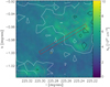 |
Fig. 1 Known structure of the environment of the mapped strip. The colors give the total gas column density derived from the Herschel SPIRE and PACS observations. The contours show the line-integrated intensity of 13CO 1−0 from the Forgotten Quadrant Survey at levels of 1.5 (white), 3.0 (gray), and 4.5 (black) K km s−1. The mapped area is shown as a red rectangle. The orange circle gives the beam and position of the existing single-pointing [C II] observation. |
2.1 Data reduction
All spectra were calibrated with the standard pipeline integrated in the APEX Control System (APECS; Muders et al. 2006). Based on the main-beam efficiencies measured on Mars and Jupiter in August to October 2024, the spectra were calibrated from antenna temperatures to main-beam temperatures using a forward efficiency of 0.985 and main-beam efficiencies at 230 and 490 GHz of 0.8 and 0.6, respectively. The efficiency uncertainties are slightly lower than 10%. This should be taken into account as a systematic uncertainty of the data. No baseline subtraction except for a constant offset (i.e., a zero-order baseline subtraction) was needed.
Using Gaussian kernels, we resampled the spectra to different spatial-spectral grids. For the plotting, all results were resampled to a common grid in RA–Dec with a resolution of 29.7 arcsec, which is 10% higher than the telescope resolution at 220 GHz, and a spacing of 6.75 arcsec. For the quantitative analyses in Sect. 4, we resampled to a uniform grid with a sampling of 4.2 arcsec parallel and perpendicular to the strip direction and the same effective resolution of 29.7 arcsec. To investigate the spatial variations in the [C I] line in Appendix A, we resampled the data to a resolution of 14.3 arcsec and kept the spacing of 4.2 arcsec. To reduce the noise in the data, the data were all spectrally resampled to a common velocity resolution of 0.25 km s−1. The investigated data cubes had a mean RMS noise level at the main-beam temperature scale of 11 mK for C18O 21 and 13CO 2−1, 12 mK for CO 2−1, and 47 mK for [C I] at a resolution of 29.7 arcsec and 160 mK at a resolution of 14.3 arcsec. As zero-position of all data, we defined the location of the existing GOTC+ pointing, l = 225.3, b = −1.0 in Galactic coordinates or RA = 07:10:39.8, Dec = −11:27:09 in J2000 equatorial coordinates.
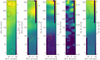 |
Fig. 2 Integrated maps of the observed strip. The left map shows the gas column density derived from the Hi-GAL observations. The circles there indicate the position and effective beam size of the spectra discussed in Fig. 4. The following maps give the line-integrated intensities of the CO 2−1, 13CO 2−1, C18O 2−1, and [C I] 1−0 transitions. The colors represent the integrated intensity for the main velocity component from 11 to 17 km s−1. The black and white contours show the integral over the component from 18 to 22 km s−1, and the orange and red contours show the integral from 34 to 38 km s−1. The zero position in the plots is at RA(J2000) = 7:10:39.8, Dec(J2000) = −11:27:09. |
2.2 Complementary data
The total column density of the region based on dust emission was retrieved from the HiGAL-PPMAP online database2, which translated all Herschel Hi-GAL data of the Galactic Plane (Molinari et al. 2010) into dust temperatures and column densities per temperature bin using the PPMAP algorithm (Marsh et al. 2015, 2017). The measured dust opacity was translated into gas column densities using a fixed opacity of 0.1 cm2/g at 300 µm, and the result is given in terms of the column density of hydrogen molecules. To avoid any assumption about the molecular state of hydrogen, we used the more general definition NH = N(H) + 2N(H2), which effectively multiplies the PPMAP data by two. The maps have a spatial resolution of the reconstructed column density of 12 arcsec.
CO 1−0 and 13CO 1−0 data were taken from the Forgotten Quadrant Survey (Benedettini et al. 2020, 2021). They have a spatial resolution of 55 arcsec and a spectral resolution of 0.3 km s−1. The CO 1−0 data have an RMS noise level of 0.8 K at this resolution in our region. For the 13CO 1−0 data, we measured an RMS noise level of 0.4 K.
The [C II] data were retrieved from the GOTC+ project (Pineda et al. 2013), which performed Herschel/HIFI observations at a spatial resolution of 12 arcsec at a single pointing next to our strip. Data were provided at the main-beam temperature scale and at a velocity resolution of 0.8 km s−1.
3 Results
Figure 2 shows the line-integrated intensity maps for the four newly observed transitions, CO 2−1, 13CO 2−1, C18O 2−1, and [C I] 1−0, in comparison to the dust-based column density map. The different velocity components identified in Fig. 3 are shown through different plotting styles. The integrated intensity of the main velocity component is given in colors. The black and white contours show the 20 km s−1 component, and the orange and red contours show the 36 km s−1 component. The contours are drawn at 50% and 80% of the peak intensity. Lacking contours indicate that the component was not detected above the noise limit.
The dynamic range covered by the different tracers is very different. While the dust column density only changes by about a factor of two along the strip, C18O 2−1 extends from a nondetection at the 10 mK km s−1 level at the one end to 0.45 K km s−1 in the brightest spots. CO 2−1 and [C I] 1−0 cover a dynamic range of a factor of about three, while 13CO 2−1 changes by more than a factor of ten across the map. Thus, [C I] 1−0 shows the smoothest spatial distribution of all considered tracers and their transitions. This is confirmed by the high-resolution analysis in Appendix A. The dust-based column density and the 13CO 2−1 and C18O 2−1 intensity distributions are significantly more patchy. Whether there is a significant difference in this aspect between the 13CO 2−1 and C18O 2−1 maps cannot be judged because the signal-to-noise ratio in the C18O 2−1 data is limited.
Figure 3 shows the position-velocity diagrams for the different lines, averaged over the pixels perpendicular to the strip. The main velocity component around 14 km s−1 is visible in all tracers, but it is only detected in C18O 2−1 at the dense end of the strip. Two other velocity components are detected. CO 2−1 and [C I] show a line at about 20 km s−1. This is more prominent in [C I] than in CO 2−1. CO 2−1 and 13CO 2−1 show another component at 36 km s−1 at offsets between 60 and 120 arcsec.
Based on the velocity of the components, we can attribute them to clouds at different kinematic distances using the Galactic rotation curve. From the kinematic distance tool by Wenger et al. (2018a), based on the rotation curve from Reid et al. (2014) and the methods described in Wenger et al. (2018b), we obtain a distance of 1.0 kpc for the 14 km s−1 component, a distance of 1.5 kpc for the 20 km s−1 component, and a distance of 2.8 kpc for the 36 km s−1 component. At a Galactic longitude of 225 degrees, these values need to be multiplied by 0.71 when they are added to the solar Galactocentric radius of 8.34 kpc (Reid et al. 2014) to obtain the Galactocentric radius of the sources.
An increase in the Galactocentric radius by up to 2.0 kpc could lead to measurable changes in the metallicity and isotopic ratios in the gas, thereby affecting our analysis of the observations and the expected structure of the PDRs. Using the range of metallicity gradients fit by Cheng et al. (2012) and Lemasle et al. (2018), we found that the metallicity in the Galactic mid-plane may drop by 17–26% for the 36 km s−1 component, but only by 6–10% for the 14 km s−1 component. The drop in metallicity should be reflected in a lower dust content of the gas, which would lead to a slightly lower dust extinction per gas column and would thereby increase the ratio of the surface tracers, such as [C II] and [C I], relative to the molecular species, such as the CO isotopologs, in the PDRs (Bolatto et al. 1999; Röllig et al. 2006). Next to the metallicity, the 12C/13C isotopic ratio changes. Based on the range of fitted gradients obtained by Yan et al. (2023) and Milam et al. (2005), the 12C/13C ratio may increase by 15–20% for the 36 km s−1 component and by 5–7% for the 14 km s−1 component. As a consequence, the 13CO intensity relative to that of CO can be somewhat lower than predicted by PDR models for solar metallicity because of the lower self-shielding of 13CO and because of the somewhat lower 13C abundance in fully molecular gas. The effect is only expected to be moderate, however. For the oxygen isotopologs, Zhang et al. (2020) found no significant systematic change on the scales considered here. This is consistent with the theoretical estimates of Henkel & Mauersberger (1993). Altogether, we should consider weak but measurable effects for the 36 km s−1 component. For most of the emission in the observed strip, which is attributable to the 14 km s−1 component, the changes should be of the order of the calibration accuracy. Thus, a comparison with models using the ISM abundances at the solar Galactocentric circle is still justified. The same applies to the weak 20 km s−1 component.
For a comparison of the velocity profiles, we show in Fig. 4 the observed spectra at three selected positions. The left plot shows the spectra at the start of the strip. The central plot shows the spectra at the location of the peak of the 20 km s−1 component (see Fig. 2), and the right plot shows those for the central pixel at the high column density end of the strip. The plots also show the CO 1−0 and 13CO 1−0 spectra from the FQS (Benedettini et al. 2020). However, they were measured at a lower resolution of 55 arcsec, so that the beam filling can be different from the other lines.
In all three positions, the intensity ratio is relatively fixed at about two between CO 2−1 and [C I] 1−0. The line profiles are very similar, but we find a hierarchy of line widths. The CO lines have a typical line FWHM of 1.6 km s−1, the [C I] 1−0 line has an FWHM of 1.4 km s−1, and the 13CO 2−1 line is narrower, with an FWHM of 0.95 km s−1, where detected. The C18O 2−1 line seems to be even narrower, but this is difficult to quantify because the signal-to-noise ratio of the line is low. It is obvious that the C18O 2−1 to 13CO 2−1 line ratio varies strongly throughout the strip. The 13CO 1−0 line is somewhat weaker than the 2−1 transition, but the low signal-to-noise ratio again makes a quantitative comparison difficult here. The 20 km s−1 component is only visible in CO 2−1 and [C I] 1−0. [C I] 1−0 shows it at all three positions, and CO 2−1 shows it only at the high column density end of the strip.
To judge to which degree the [C II] GOTC+ spectrum (Pineda et al. 2013) can be taken as representative for our strip, we show in Fig. 5 the spectra of CO 1−0 and 13CO 1−0 for the GOTC+ position together with the [C II] spectrum. We recall that they were measured at a different resolution, so that they cannot be quantitatively compared. In [C II], we only have a non-detection or tentative detection, with a maximum line-integrated intensity of 0.2 K km s−1. This corresponds to 1.4 times the baseline noise at the resolution of the line width of 1.5 km s−1. The profile of CO 1−0 with an integrated intensity of 8 K km s−1, the nondetection of 13CO 1−0, and the dust-based column density of 3.4 × 1021 cm−3 all match the observations within the lower 80 arcsec of our strip. Hence, we consider the upper limit of 0.2 K km s−1 for the [C II] intensity as representative for the low-column-density end of our strip.
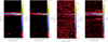 |
Fig. 3 Position-velocity diagrams for the four observed lines: CO 2−1, 13CO 2−1, C18O 2−1, and [C I] 1−0 (from left to right). All spectra are averaged in the direction perpendicular to the observed strip. |
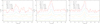 |
Fig. 4 Spectra measured at three selected positions. The left plot shows the zero-position of the map, the central plot shows the peak of the 20 km s−1 component, and the right plot shows the central pixel at the bright end of the strip (see Fig. 7). The individual spectra have been shifted vertically by 2 K relative to each other to improve the visibility. As the 36 km s−1 component is not detected above the noise level for these three positions, the plotted spectral range is limited to the other two velocity components. |
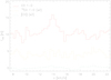 |
Fig. 5 Spectra of CO 1−0, 13CO 1−0, and [C II] at the position of the GOTC+ observations next to our strip. The CO and 13CO 1−0 profiles have been shifted in the same way as in Fig. 4 to allow for a direct comparison. |
4 Correlations
To verify whether our [C I] data follow the often observed tight correlation to the 13CO emission, we studied the correlation between the [C I] emission and the other tracers within the position-velocity cubes. Figure 6 shows the distribution of intensities within the frequency windows of the velocity components with significant emission. The first four panels cover the main emission component between 11 and 17 km s−1. The last two panels show the corresponding distributions for the two other velocity components in the lines that were detected above the noise level. The distributions are shown as probability density functions (PDFs) of the spectral pixel intensities, where we subtracted the PDFs of the noise contribution by measuring the latter in channels outside of the line window. Therefore, the plots should represent actual emission only.
In the main velocity component, the relation between 13CO 2−1 and [C I] 1−0 (second panel) is clearly not at all linear, while the relation between CO 2−1 and [C I] 1−0 (first panel) follows a linear trend despite very different optical depths (see Sect. 5.2). This is consistent with the relation between 13CO 2−1 and CO 2−1 being nonlinear. The relation between 13CO 2−1 and C18O 2−1 also follows a linear trend, but there seems to be some excess of C18O 2−1 at a level of up to 2σnoise for low levels of 13CO 2−1. In contrast to the 14 km s−1 component, the 36 km s−1 component shows a quite linear trend between 13CO 2−1 and CO 2−1. For the 20 km s−1 component, it is remarkable that we find significant [C I] 1−0 emission at a 3.5σnoise level in spectral pixels with no or very little CO 2−1 emission, indicating the presence of CO-dark gas with atomic carbon.
To characterize typical line ratios, we fit the relations between the different intensities by a linear model that accounted for uncertainties in both axes using the LINFITEX function (Press et al. 1992) implemented in the MPFIT package3 from Markwardt (2009). The results are given in Table 1 and the fits are overplotted in Fig. 6. It is clear that except for the CO 2−1/[C I] 1−0 relation, linear fits are a poor representation of the observed behavior. The uncertainty in the linear fit is typically very small due to the large number of spectral pixels compared, but it gives no indication of the quality of a linear model. Therefore, we do not only give the parameter uncertainties from the fit, but also computed the scatter of the measured intensities around the fitted line. This is expressed as the intercept and slope of a linear description of the standard deviation of the distribution of values around the fitting line.
Next to the relations for the line ratios, Table 1 also shows the linear fit results when comparing the lines with the total column density. Here, the line intensities were integrated over all velocity components. The line-intensity ratios show that only two relations have a nonzero intercept within the uncertainties: the relations between 13CO 2−1 and either CO 2−1 or [C I] 1−0. This shows that a significant intensity of CO 2−1 and [C I] 1−0 has to build up before the formation of 13CO sets in. A similar effect is expected for C18O, but the uncertainties are larger there because the detection is weak.
For the relations of the line-integrated intensities to the dust-based column, we can translate the intercept to the column density for which the line intensity becomes positive by dividing the negative intercept by the slope. In this way, we obtained a minimum column density for the formation of CO and [C I] of 2.3 × 1021 cm−2, for 13CO of 3.6 × 1021 cm−2, and for C18O of 4.2 × 1021 cm−2. Because of this intercept, the slope of the fitted line must not be mixed with the typical ratio of the two quantities that is discussed below. As the line only starts above the formation threshold, the slope is higher between two and almost ten times than the mean ratio over the map (Table 2).
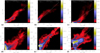 |
Fig. 6 Distribution of line intensities based on a comparison of different transitions at the same spatial-spectral pixel. The panels compare (a) CO 2−1 to [CI] 1−0, (b) 13CO 2−1 to [CI] 1−0 (c) CO 2−1 to 13CO 2−1, (d) 13CO 2−1 to C18O 2−1, for the 14 km s−1 component, i.e., all spectral pixels in the line window from 11 to 17 km s−1, (e) CO 2−1 to 13CO 2−1 in the 36 km s−1 component (340–38 km s−1), and (f) CO 2−1 to [CI] 1−0 for the 20 km s−1 component (18–22 km s−1). The noise distribution determined outside of the spectral window is subtracted to emphasize the relation for true emission only. The white line and the equation at the top show the results of a linear fit to all noise-weighted points forming the distributions. |
Linear fit parameters for the relations between the different line intensities.
5 Modeling
5.1 Line ratios
To determine the physical parameters of the main gas component, we considered intensities averaged in the direction perpendicular to the strip and integrated over the 14 km s−1 line. They are plotted in Fig. 7 together with the column density profile from the dust observations. As already discussed in Sect. 3, the [C I] line varies least across the strip, being similar to the dust profile, while all molecular lines show stronger variations with bumps in the CO isotopolog lines around 160 and 250 arcsec offset and significant emission in 13CO 2−1 and C18O 2−1 only at offsets above 100 arcsec.
For an estimate of the column of the different species, we considered the intensities integrated over the main velocity component. For a physical model of the gas in terms of a PDR, we did not fit absolute intensities, but considered ratios that characterized the line emission efficiency of a gas column. On the one hand, we used the line intensities relative to the total gas column, NH. On the other hand, we used the intensities relative to the CO 2−1 line intensity, which characterize the emission efficiency of the molecular gas alone. In Table 2, we list the mean, minimum, and maximum values and ratios along the strip used in the subsequent modeling as they are read from Fig. 7.
Mean, minimum, and maximum values for column density and the different intensities and intensity ratios integrated over the main velocity component and averaged perpendicular to the observed strip.
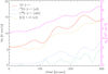 |
Fig. 7 Comparison of the line-integrated intensities of [C I] and the CO isotopologs (left axis) with the column density along the strip (right axis, purple). All data are averaged perpendicular to the strip direction. |
5.2 Uniform slab approximation
In a first approach, we tried to analyze the observed intensities in the frame of a uniform medium characterized by the parameters density, kinetic temperature, column density within the telescope beam, beam-filling factor, and the abundance of the individual species. The total column density of gas is constrained by the dust observations, but this still leaves three free parameters plus one for each observed molecule. Unfortunately, our observational constraints from the line intensities are insufficient to derive this number of parameters as we have two lines per species at most. Hence, we made some simplifying assumptions. The general assumption that we applied here is a beam filling of unity. This means no breaking up of the material on the scale below the telescope beam. This is well justified by the smoothness of the intensity distribution in all tracers and the smooth distribution of the [C I] map at the even higher resolution shown in Appendix A.
The next approximation can be made by assuming local thermodynamic equilibrium (LTE), so that the derived abundances become independent of the gas density. Unfortunately, the LTE approximation was found to be invalid in our case. We used the ratio of the 13CO 2−1 and 1−0 lines to measure the excitation temperature without optical depth effects. It varies between 0.6 and 0.8 across our strip. The 1−0 transition is only measured at a coarser resolution than the rest of the data (see Sect. 2.2), but as all maps are relatively smooth, this might still give reasonable results. However, the ratio translates into an excitation temperature of only 5–6 K (Mangum & Shirley 2015), which is much lower than the typical kinetic temperature in diffuse interstellar gas or molecular clouds (Tielens 2005). The value also contradicts the observed peak intensity of the CO line, which falls at about 8 K, corresponding to a Rayleigh-Jeans-corrected excitation temperature of about 13 K in an optically thick line. This provides a lower limit to the actual excitation temperature. The observed gas is clearly not in LTE. This indicates that the gas is at densities below the critical density for the 2−1 transition of about 7000 cm−3 (Ossenkopf 2000).
From the combination of the 1−0/2−1 ratios of the CO and 13CO transitions with the line intensities, we can instead derive all four physical parameters (the gas temperature and density, and the columns of CO and 13CO) for a uniform beam filling of all lines. We used the non-LTE molecular radiative transfer code RADEX (van der Tak et al. 2007) to simulate the line intensities and perform a least-squares fit to the observed mean intensities from Table 2. We used the velocity dispersion FWHM of 0.95 km s−1 as measured for the 13CO lines and the escape probability formalism for a spherical configuration (Ossenkopf 1997), and we assumed that H2 is the main collision partner in the gas and dominates the collisional excitation. The fit of the intensities computes a four-dimensional χ2 distribution in the space of parameters that we defined as kinetic temperature, H2 density, 13CO column, and CO/13CO abundance ratio. The minimum gives the numerically best solution.
Figure 8 shows two-dimensional cuts through the four-dimensional χ2 surface. This measures the match of the observed intensities and the values simulated by RADEX. All cuts were taken at the location of the χ2 minimum. The χ2 values are given on a logarithmic scale. Because values on the order of unity (shown in blue) indicate a valid solution, this describes a small spot in the parameter area. The parameters are well constrained, even better than needed for a general assessment of the typical behavior within our strip. For a physical understanding of the observational constraints, we added four contour lines to indicate the parameter combinations where the observed values are matched. The black and white lines stand for the integrated intensities of CO 2−1 and 13CO 2−1. The ratios of CO 1−0/CO 2−1 and 13CO 1−0/13CO 2−1 are shown as red and brown lines, respectively. A crossing of all lines in one point would indicate the perfect solution. The plots show that the kinetic temperature of the gas is best constrained by the CO 2−1 intensity, the gas density by the 13CO 1−0/13CO 2−1 ratio, and the total column density and the CO/13CO column density ratio by the CO 2−1 intensity and the CO 1−0/CO 2−1 ratio.
The χ2 minimum is met for an H2 density of 1000 cm−3, a kinetic gas temperature of 20.5 K, a 13CO column density of 1.6 × 1015cm−2, and a CO/13CO abundance ratio of 70. At this column, even 13CO turns slightly optically thick, with a line-center optical depth of 0.3 and 0.7 for the 1−0 and 2−1 transition, respectively. Using the density and temperature obtained from CO and 13CO, we determined the mean [C I] 1−0 intensity of 2.9 K km s−1 in the RADEX grid and read a column of atomic carbon of 6.2 × 1016 cm−2 and an optical depth of the 1−0 line of 0.6. We translated the columns of CO and atomic carbon into a total gas column using the total gas-phase carbon abundance of X(C)/X(H) = 2.34 × 10⁻⁴ (Simón-Díaz & Stasinska 2011), and we obtained NH = 4.7 × 1020 cm−2 for the gas traced by CO and NH = 2.6 × 1020 cm−2 for the gas traced by [C I]. This is only about 20% of the total column as measured through the dust emission. About the same amount of gas can be hidden in ionized carbon within the upper limit of the [C II] line intensity of 0.2 K km s−1 for the same excitation conditions, but this still leaves about half of the total gas column unexplained. As the ratios of the lines and the dust-based column density vary only weakly along the strip, this ratio is independent of the exact location in the strip.
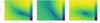 |
Fig. 8 Two-dimensional cuts through the χ2 topology of the RADEX simulation of the observed intensities of the CO 1−0, 2−1 and 13CO 1−0 and 2−1 lines. The χ2 values are given in logarithmic units, so that only the dark blue area indicates a valid fit. All slices are taken through the χ2 minimum. The contour lines show the parameters at which the observed values were matched. The black and white lines show the integrated intensities of CO 2−1 and 13CO 2−1, and the red and brown lines show the ratios of CO 1−0/CO 2−1 and 13CO 1−0/13CO 2−1. |
5.3 PDR modeling
Instead of deriving individual abundances of the different species, we compared the observed intensities with a chemical PDR model that self-consistently predicted all abundances and excitation temperatures as a function of fewer parameters. A number of PDR models is available for this type of astrochemical modeling of the region (see e.g. Röllig et al. 2007; Wolfire et al. 2022). Most of the models assume a one-dimensional infinite slab in a plane-parallel geometry. Instead, we used the KOSMA-τ PDR model (Röllig & Ossenkopf 2013; Röllig & Ossenkopf-Okada 2022), which tries to represent the high importance of surfaces by switching to a spherical configuration or a superposition of many spherical clumps, thus exhibiting a larger surface-to-volume ratio than the plane-parallel models. In this way, we expected to match the observed high [C I]/CO intensity ratio in our region better, which indicates a large fraction of dissociated gas in UV-illuminated surface layers. Moreover, KOSMA-τ includes the full isotopic chemistry, which allowed us to also compare the abundances of 13CO and C18O. The model assumes a radial density gradient with a central density that is about ten times higher than the surface density that we give as parameter in the figures here.
We did not perform a combined χ2 fit of all observed ratios, but instead inspected the behavior of the different ratios in a model grid spanning a range of surface densities and clump masses to constrain the conditions under which the observed ratios were reproduced. As there are no bright UV sources in the vicinity of our region, we kept the normal impinging UV flux measured in the solar neighborhood of one Draine field, (χD = 8.96 × 10⁻¹⁴ erg cm−3, Draine & Bertoldi 1996). In Appendix B, we show the corresponding results for a ten times higher UV flux. This proves that none of our conclusions would change if this assumption was violated. The model grid was based on the UdfA 2012 chemical network (McElroy et al. 2013) without ice formation. All parameters are listed in Andree-Labsch et al. (2017).
Figure 9 shows the model predictions for the ratio of the five integrated line intensities relative to the column density when the clump density and mass were varied. For these ratios, the results are independent of variations in the total column density in the beam or a nonuniform beam filling, but focus on the line emissivity of the observed material. The yellow patches correspond to higher line intensities from the same column of material, and dark blue patches show low emissivities. In all of our lines, very dense and massive clumps produce only very low line emissivities because these clumps would be cold and optically thick. The strongest line emissivity is reached for the smallest clumps of only 10−3 M⊙, but the density of the peak emissivity varies strongly between the five lines. For C18O 2−1, we obtain the brightest line per column for a clump surface density of 106 cm−3, for [C II] at 103 cm−3.
The plots contain two types of contours. The white, gray and black contours represent the minimum, mean, and maximum of the observed ratios from Table 2. Not all subplots show all three contours. For 13CO 2−1, the observed minimum is not reached within the scanned parameter range, and even the mean and maximum is only predicted for the densest and most massive clumps. For C18O 2−1, even the maximum observed value falls below all model predictions, so that no contours are shown. The lowest model predictions, which are closest to the observed range, occur for the small and thin clumps in the lower left corner of the parameter range in which almost all C18O is photo-dissociated, but some CO and 13CO exist because their self-shielding is stronger. For [C II], this is the parameter range with the highest predicted intensity. However, the [C II] upper limit from the possible tentative detection, indicated by the black line, excludes all the high emissivities predicted by the model in the left lower part of the parameter range.
The second type of contours, the red and orange lines, indicate model parameters for which the column densities observed in the strip match the column densities of the individual model clumps. This is not a strict constraint on the models. In parameter regions in which the model column density falls below the observed column density (lower left corner), the observed column might be the sum of multiple clumps along the line of sight at the same velocity. If the model clump column density exceeds the observed column (upper right corner), only part of the clumps might fall into the beam, so that the measured column density within the telescope beam falls below the clump column. This is reasonable for the massive low-density clumps in the upper left corner of the parameter range, where the physical size of the model clumps exceeds the beam width at 1.0 kpc distance. However, the narrow line width and the smooth distribution of the emission across the map even at the best resolution indicate that both effects probably play only a minor role, so that the region selected by the two lines is at least an approximate guideline.
Figure 10 again shows model ratios of the different integrated-line intensities, but this time, relative to the CO 2−1 intensity. In this way, we characterize the CO-bright molecular gas alone. The CO 2−1 intensity itself is shown in the left panel. The relatively low absolute intensity of CO 2−1 indicates gas at moderate densities of 103–104 cm−3, but only a very weak sensitivity to the clump mass is visible. The [C I] 1−0/CO 2−1 ratio suggests the same low densities, regardless of the clump mass. The measured low ratios of 13CO 2−1/CO 2−1 and C18O 2−1/CO 2−1 further constrain the parameter range by also asking for low densities, but additionally excluding all massive clumps. This contradicts the low measured [C II]/CO 2−1 ratio that excludes all low-density models and requires densities of at least 104 cm−3.
Based on a combination of the information, we have to conclude that all models are invalid for our region. When we only consider CO, [C I], and the total gas column, models with low density and masses around 100 M⊙ would fit the data. In contrast, both 13CO 2−1 and C18O 2−1 require models where the molecules are dissociated and mainly consist of atomic gas. They are simulated by models with low mass and density. in contrast, the low [C II] intensity observed in the field is only consistent with mainly molecular gas that requires high densities. Models for a higher UV field (Appendix B) show that this incompatibility is independent of the UV field; a higher UV field only shifts all lines for 13CO 2−1, C18O 2−1, and [C II] toward higher clump masses and densities, but creates no overlap.
These tests stress that a blind χ2-fit of the observational data by the models would be rather misleading. It would hide the fundamental mismatch. It is also easy to see why switching to a plane-parallel model does not solve the problem: Lowering the surface relative to the volume decreases photo-dissociation of 13CO 2−1 and C18O 2−1, so that it would drive their line ratio relative to CO 2−1 further up, creating an even larger mismatch to the observations.
In contrast, it might be possible to construct a PDR model that simultaneously fits the 13CO 2−1, C18O 2−1, and [C II] observations by using a much lower UV field that would result in very cold clouds. A very low UV field due to some preshielding gas was already proposed as a solution to PDR model mismatches by Bensch et al. (2003), but as discussed in Schneider et al. (2024), it is very unlikely to find a UV field much below the Draine field in the Galactic plane. Hence, we did not create models for these conditions. This can be a possible approach for follow-up investigations.
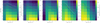 |
Fig. 9 Integrated line intensities predicted by the KOSMA-τ PDR model relative to the column density of the model clumps. The panels from left to right show CO 2−1, 13CO 2−1, C18O 2−1, [C I] 1−0, and [C II]. The white, gray, and black lines indicate the minimum, mean, and maximum of the observed ratio. For [C II], we only have an upper limit. For C18O 2−1, even the maximum falls outside of the covered parameter range and is lower than all displayed values. The red and orange contours indicate the lowest and highest column density in the region obtained from the dust observations. |
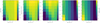 |
Fig. 10 Integrated line intensities predicted by the KOSMA-τ PDR model relative to the CO 2−1 intensity. The left panel shows this CO 2−1 intensity, and the subsequent panels give the ratios for 13CO 2−1, C18O 2−1, [C I] 1−0, and [C II]. The white, gray, and black lines indicate the minimum, mean, and maximum of the observed ratios. |
6 Discussion
Qualitatively, the intensity profiles of the CO isotopologs follow the expected sequence, where isotope-selective photodissociation due to different columns of self-shielding molecules lead to the sequence of CO formation at relatively low column densities of attenuating dust, 13CO formation at higher columns, followed by C18O formation at even higher columns. The correlation analysis in Sect. 4 indicates a critical visual extinction of AV = 1m.2 for the formation of CO, AV = 1m.9 for the formation of 13CO, and AV = 2m.3 for C18O4. Figure 7 shows that the onsets of emission from 13CO and C18O fall within the observed strip. However, when we compare these numbers with the predictions from the model grids introduced in Sect. 5.3, there are no good matches. Depending on the model parameters, the critical columns for the formation of the CO isotopologs vary slightly, but they all fall in the range around AV = 1m.0, and the spread between the three isotopologs covers less than AV = 0m.3. Hence, the effective column shielding the gas against the UV radiation must be significantly lower than the column measured along the line of sight. This can be explained either by a significant contribution of unrelated diffuse interstellar gas to the measured dust column (see below), or by the typical geometric difference between the effective UV shielding column, AV,eff in a turbulent three-dimensional configuration and the line-of-sight column, AV. Seifried et al. (2020) found AV,eff ≈ 1/3 AV for a set of hydrodynamic and magnetohydrodynamic simulations of the turbulent ISM within the SILCC-Zoom project (Walch et al. 2015; Seifried et al. 2017). However, in both cases, we still cannot explain why the spread between the isotopologs in our observations is much larger than in the models.
Our radiative transfer analysis showed a discrepancy between the gas column obtained from the different carbon-bearing species and the column derived from the dust emission for uniform excitation conditions in the gas. Counting the carbon in the gas phase provided less than half of the column measured through the dust emission. Consequently, our methodical assumptions need to be questioned. As discussed above, there is no chemically homogeneous configuration. Instead, we should see a layered structure with ionized carbon at the cloud surface that is only weakly shielded from the interstellar radiation field, then, atomic carbon and CO at intermediate depths, then 13CO, and finally, C18O deepest within the clouds, typically also associated with the highest densities. This is consistent with the fact that the measured CO/13CO abundance ratio of 70 is slightly higher than the value obtained from Langer & Penzias (1993) and Wilson (1999) for a Galactocentric radius of 9 kpc for the 14 km s−1 component (see Sect. 3). However, the solution in Fig. 8 for the impact of a density variation between 13CO and CO shows that the dependence is very weak. The conclusion is even stronger for the [C I] 1−0 line. Its emissivity per carbon column is quite constant over a wide range of temperatures and densities. Papadopoulos et al. (2022) have shown that for a wide range of ISM conditions ( cm−3 and Tkin = 20–80 K), the [C I] 1−0 emissivity changes by only 20%. The only explanation for the discrepancy in the frame of chemical differentiation of the region is some diffuse envelope or line-of-sight contamination with densities as low as 10 cm−3. In this gas, all carbon would be in the form of C+, but its collisional excitation is too low to make it visible in the [C II] line (Goldsmith et al. 2012). In this scenario, only half of the visible column density in the dust emission would be associated with the observed gas, while the other half stems from the diffuse medium. Unfortunately, this explanation contradicts the low dust temperature determined in the region. The PPMAP analysis (Marsh et al. 2017) shows most of the dust at temperatures around 15 K, which is much colder than dust in diffuse clouds.
This leads to an alternative explanation, however: gas freeze-out. The gas-phase abundances used here were calibrated for the Orion molecular cloud (OMC1; Simón-Díaz & Stasinska 2011). Dust temperatures of 15 K are significantly colder than in active star-forming regions such as OMC1, so that we might assume that half of the carbon from the gas phase is frozen onto the grains. This is consistent with the temperature dependence of the C18O depletion factor measured by Lewis et al. (2021) in the California cloud. A resulting gas-phase abundance as low as X(C)/X(H) = 1.2 × 10⁻⁴ would provide an alternative explanation for the discrepancy. However, Lewis et al. (2021) found a stronger depletion for 13CO, while we see a significant under-abundance of C18O. Moreover, PDR models predict freeze-out only deep in the clouds, not close to the surface where C18O just starts to form. We conclude that both explanations are so far questionable.
Benedettini et al. (2020) compared the CO 1−0 and 13CO 1−0 intensities with the dust-based column densities and obtained conversion factors between CO intensity and H2 column corresponding to CO 1−0/NH = 1.5 × 10⁻²¹ K km s−1 cm2 and 13CO 1−0/NH = 4.2 × 10⁻²² K km s−1cm2 for the FQS. Our values of 2.6 × 10⁻²¹ K km s−1cm2 and 3.2 × 10⁻²² K km s−1cm2 for the two ratios (Table 2) deviate in opposite directions, indicating that our field is not representative for the whole region. The strip is relatively CO-bright compared to the whole FQS area, while it is still only weakly shielded, so that 13CO is less abundant. If the good correlation between [C I] 1−0 and the CO transitions holds for the full area of the FQS, this would suggest a significant and extended [C I] brightness from this part of the Galaxy.
In contrast to many previous observations, we observed a relatively high intensity of the [C I] line when compared to CO. Our fits of the line ratios provided a [C I] 1−0/CO 2−1 ratio (in K km s−1) of 0.27 and a [C I] 1−0/13CO 2−1 ratio of 1.6 for the 14 km s−1 component. For the 20 km s−1 component, the [C I] 1−0/CO 2−1 ratio even increased to 2.6. For the Orion A cloud, Arunachalam (2023) and Labkhandifar (2023) found typical ratios for [C I] 1−0/13CO 2−1 of about 0.3 and for [C I] 1−0/CO 2−1 of about 0.05. Lee et al. (2022) measured for the ATLASGAL clumps a mean ratio [C I] 1−0/13CO 2−1 of 0.56 and a tendency toward higher ratios for less evolved clumps. Their sample of 35 diffuse clumps showed a mean ratio of 1.0. Aligning our results with these data, we see a clear trend from low ratios of [C I] 1−0 and the molecular lines for dense evolved regions, harboring active star formation, to high ratios for diffuse clouds at low radiation fields. In this sequence, our observations currently provide the low-density end with the highest ratios.
This is in line with unresolved observations of whole galaxies. Topkaras et al. (2024) determined by integrating over whole galaxies for a large number of extragalactic observations a typical ratio of the integrated intensities [C I] 1−0/CO 1−0 ≈ 0.22 or [C I] 1−0/CO 2−1 ≈ 0.26, respectively. This is five times higher than the Galactic value for the bright regions, but it is in line with our number for the 14 km s−1 component and below the ratio measured in the 20 km s−1 component. When integrating over a whole galaxy that always contains a mixture of dense and bright regions with diffuse gas, the atomic carbon is predominantly seen from the diffuse regions. The [C I] emission from galaxies is dominated by material at moderate densities around 103 cm−3, not by the small bright cores. In this sense, it seems worth reconsidering low-resolution single-dish mapping observations of the Milky Way and nearby galaxies, and not focusing on the new capabilities of modern interferometers alone.
Future observations should examine the 20 km s−1 component, in which the [C I] emission exceeds that of CO. We speculate that this indicates a large fraction of CO-dark molecular gas in this component. Unfortunately, the GOTC+ observations did not cover the component, and high-resolution H I absorption observations are not available yet either. A large fraction of the CO-dark molecular gas may be traced rather by [C I] emission than by [CII] (see Pineda et al. 2013). As [C II]-based investigations already showed fractions of CO-dark molecular gas between 20% and 80% (e.g. Langer et al. 2014; Xu et al. 2016; Chen et al. 2015), the actual amount of molecular material that is not traced by the standard CO observations may be significantly higher. The combination of the existing knowledge about an increasing fraction of CO-dark molecular gas with increasing Galactic latitude (Luo et al. 2024; Xu et al. 2016) with our indications of CO-dark molecular gas even in the Galactic midplane traced through [C I] emission suggests that we may still miss a significant fraction of the Milky Way ISM in all observations performed until today. This is a strong justification for the science case of the GEco survey, which will map large areas in the Galaxy.
7 Conclusions
When regions of the Milky Way are mapped that are not prominent star formation sites, several of the relations calibrated for the massive star-forming regions break down. By selecting one such inconspicuous region for a detailed mapping in [C I] 1−0 and the different CO isotopologs, we found that the detected gas fraction in CO is rather low. A significant fraction of the gas is traced through [C I], leading to a [C I] 1−0/CO 2−1 ratio that can be as high as 2.6 for our 20 km s−1 component. This might indicate CO-dark molecular gas, but a clear assignment requires better H I data. Unfortunately, the sum of the carbon-bearing gas seen in the CO isotopologs, [C I], and ionized carbon, visible through [C II] emission, falls short of the column measured by dust emission by about a factor of two when we assume a gas density around 103 cm−3, which is consistent with the observations of [C I], CO, and 13CO.
The optical depth of the [C I] 1−0 line is similar to that of the 13CO lines, but the spatial distribution is very different due to the layering structure of PDRs. In contrast, we found a very close correlation to the intensity distribution of the CO lines and a match to their line width, although the optical depth of the CO lines is far higher. This indicates that neither CO nor 13CO follow the abundance of atomic carbon in translucent clouds. Atomic carbon must be more extended both spatially and in velocity space. Large-scale mapping of [C I] in the Milky Way, including the unimpressive but statistically important diffuse regions, is therefore essential for deriving the correct distribution of atomic carbon in our Galaxy. This is the goal of the planned GEco project at CCAT/FYST, which will map the Milky Way in [C I].
Qualitatively, our observations seem to confirm the astro-chemical models predicting a layering of species in PDRs. They show the expected sequence with extended [C I] and CO, 13CO, and C18O above different critical column densities that govern the self-shielding of the molecules. Quantitatively, however, we note significant mismatches. The models predict a smaller separation between the onsets of CO, 13CO, and C18O emission, and they predict either more [C II] emission than observed (in the case of diffuse gas) or more C18O emission than observed (in the case of dense gas). This indicates some fundamental deficiency in the current PDR modeling or some so-far overlooked mechanism of additional UV attenuation.
It is impossible to draw any statistical conclusion from the tiny strip observed here. It fits into a consistent picture for the [C I] emission from galaxies in which the emission integrated over a whole galaxy represents a mixture of bright and diffuse regions, however. Bright regions, which were the focus of most previous studies, only contribute little to the total [C I] emission, while more diffuse gas such as we observed here dominates the sum.
Acknowledgements
We thank Arnaud Belloche for help with the preparation of the observations and their execution. We thank Markus Röllig for many useful discussions. This work is supported by the Collaborative Research Center 1601 (SFB 1601 sub-projects A1, A6, and B2) funded by the Deutsche Forschungsgemeinschaft (DFG, German Research Foundation) – 500700252.
Appendix A [C I] at the full spatial resolution
The APEX resolution of 13 arcsec at 492 GHz allows us to study spatial variations at smaller scales than for the other tracers. Figure A.1 (left) shows the integrated line map, equivalent to Fig. 2, at a spatial resolution of 14.3 arcsec. Some small scale variations are visible, but they can be partly due to the noise in the data, not tracing actual variations. Therefore the right hand side shows a plot that gives the difference map between this 14.4 arcsec map and the map smoothed to the 29.7 arcsec of Fig. 2. As the noise level of the integrated lines is 0.2 K km s−1 we can conclude that most of the spatial variations can just be due to noise. Overall the high resolution data are consistent with the smooth [C I] distribution discussed in Sect. 3.
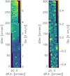 |
Fig. A.1 Integrated [C I] map at a resolution of 14.3 arcsec (left) and difference to the low-resolution map from Fig. 2 (right). Colors give the integrated intensity for the 14 km s−1 component, contours show the 20 km s−1 -component. |
Appendix B Models for an elevated radiation field
As there are no bright sources known in the vicinity of the considered cloud we expect that the standard UV field in the solar neighborhood also applies there. However, as the GAIA data are incomplete for embedded massive stars, there is a chance to find an elevated UV field, even if the Herschel continuum data give no hint for hotter dust. To be on the safe side, we also checked PDR models with a ten times higher UV flux in terms of the fit of the observational data. Figures B.1 and B.2 show the intensity ratios from the model grid compared to the observations in the same way as Figs. 9 and 10. We see qualitatively the same behavior. With the higher UV flux, the low observed intensities of 13CO 2−1 and C18O 2−1 are met be the smallest clumps with low densities, but the non-detection of the [C II] line is only met for models with very high densities and masses. The fundamental incompatibility of both observational constraints with the PDR modelling remains.
References
- Alaghband-Zadeh, S., Chapman, S., Swinbank, A., & et al. 2013, MNRAS, 435, 1493 [NASA ADS] [CrossRef] [Google Scholar]
- Andree-Labsch, S., Ossenkopf-Okada, V., & Röllig, M. 2017, A&A, 598, A2 [NASA ADS] [CrossRef] [EDP Sciences] [Google Scholar]
- Arunachalam, M. 2023, Master’s thesis, MPIfR Bonn and University of Cologne, Germany [Google Scholar]
- Benedettini, M., Molinari, S., Baldeschi, A., et al. 2020, A&A, 633, A147 [NASA ADS] [CrossRef] [EDP Sciences] [Google Scholar]
- Benedettini, M., Traficante, A., Olmi, L., et al. 2021, A&A, 654, A144 [NASA ADS] [CrossRef] [EDP Sciences] [Google Scholar]
- Bensch, F., Leuenhagen, U., Stutzki, J., & Schieder, R. 2003, ApJ, 591, 1013 [NASA ADS] [CrossRef] [Google Scholar]
- Bohlin, R. C., Savage, B. D., & Drake, J. F. 1978, ApJ, 224, 132 [Google Scholar]
- Bolatto, A. D., Jackson, J. M., & Ingalls, J. G. 1999, ApJ, 513, 275 [NASA ADS] [CrossRef] [Google Scholar]
- Chen, B. Q., Liu, X. W., Yuan, H. B., Huang, Y., & Xiang, M. S. 2015, MNRAS, 448, 2187 [Google Scholar]
- Cheng, J. Y., Rockosi, C. M., Morrison, H. L., et al. 2012, ApJ, 746, 149 [NASA ADS] [CrossRef] [Google Scholar]
- Dong, Y., Sun, Y., Xu, Y., & et al. 2023, ApJS, 268, 1 [NASA ADS] [CrossRef] [Google Scholar]
- Draine, B. T., & Bertoldi, F. 1996, ApJ, 468, 269 [Google Scholar]
- Glover, S. C., Clark, P. C., Micic, M., & Molina, F. 2015, MNRAS, 448, 1607 [NASA ADS] [CrossRef] [Google Scholar]
- Godard, B., Pineau des Forêts, G., La Porte, J., & Merlin-Weck, M. 2024, A&A, 689, A25 [NASA ADS] [CrossRef] [EDP Sciences] [Google Scholar]
- Goldsmith, P. F., Langer, W. D., Pineda, J. L., & Velusamy, T. 2012, ApJS, 203, 13 [Google Scholar]
- Gong, M., Ostriker, E., & Wolfire, M. 2017, ApJ, 843, 38 [NASA ADS] [CrossRef] [Google Scholar]
- Güsten, R., Nyman, L. Å., Schilke, P., et al. 2006, A&A, 454, L13 [NASA ADS] [CrossRef] [EDP Sciences] [Google Scholar]
- Henkel, C., & Mauersberger, R. 1993, A&A, 274, 730 [NASA ADS] [Google Scholar]
- Hollenbach, D. J., & Tielens, A. G. G. M. 1999, Rev. Mod. Phys., 71, 173 [Google Scholar]
- Jenkins, E., & Tripp, T. 2011, ApJ, 734, 65 [NASA ADS] [CrossRef] [Google Scholar]
- Labkhandifar, N. A. 2023, PDR-Chemie in der Orion-A Molekülwolke, Bachelor thesis, University of Cologne, Germany [Google Scholar]
- Langer, W. D., & Penzias, A. A. 1993, ApJ, 408, 539 [NASA ADS] [CrossRef] [Google Scholar]
- Langer, W. D., Velusamy, T., Pineda, J. L., Willacy, K., & Goldsmith, P. F. 2014, A&A, 561, A122 [NASA ADS] [CrossRef] [EDP Sciences] [Google Scholar]
- Lee, M.-Y., Wyrowski, F., Menten, K. M., et al. 2022, A&A, 664, A80 [NASA ADS] [CrossRef] [EDP Sciences] [Google Scholar]
- Lemasle, B., Hajdu, G., Kovtyukh, V., et al. 2018, A&A, 618, A160 [NASA ADS] [CrossRef] [EDP Sciences] [Google Scholar]
- Lewis, J. A., Lada, C. J., Bieging, J., et al. 2021, ApJ, 908, 76 [CrossRef] [Google Scholar]
- Luo, G., Li, D., Zhang, Z.-Y., et al. 2024, A&A, 685, L12 [NASA ADS] [CrossRef] [EDP Sciences] [Google Scholar]
- Mangum, J. G., & Shirley, Y. L. 2015, PASP, 127, 266 [Google Scholar]
- Markwardt, C. B. 2009, in ASP Conf. Series, 411, Astronomical Data Analysis Software and Systems XVIII, eds. D. A. Bohlender, D. Durand, & P. Dowler, 251 [Google Scholar]
- Marsh, K. A., Whitworth, A. P., & Lomax, O. 2015, MNRAS, 454, 4282 [Google Scholar]
- Marsh, K. A., Whitworth, A. P., Lomax, O., et al. 2017, MNRAS, 471, 2730 [Google Scholar]
- McElroy, D., Walsh, C., Markwick, A. J., et al. 2013, A&A, 550, A36 [NASA ADS] [CrossRef] [EDP Sciences] [Google Scholar]
- Milam, S. N., Savage, C., Brewster, M. A., Ziurys, L. M., & Wyckoff, S. 2005, ApJ, 634, 1126 [Google Scholar]
- Molinari, S., Swinyard, B., Bally, J., et al. 2010, A&A, 518, L100 [NASA ADS] [CrossRef] [EDP Sciences] [Google Scholar]
- Muders, D., Hafok, H., Wyrowski, F., et al. 2006, A&A, 454, L25 [NASA ADS] [CrossRef] [EDP Sciences] [Google Scholar]
- Ossenkopf, V. 1997, New A, 2, 365 [Google Scholar]
- Ossenkopf, V. 2000, in ESA Special Publication, 456, ISO Beyond the Peaks: The 2nd ISO Workshop on Analytical Spectroscopy, eds. A. Salama, M. F. Kessler, K. Leech, & B. Schulz, 303 [Google Scholar]
- Ossenkopf, V., Röllig, M., Cubick, M., & Stutzki, J. 2007, in Molecules in Space and Laboratory, eds. J. Lemaire, & F. Combes, 351 [Google Scholar]
- Papadopoulos, P., Dunne, L., & Maddox, S. 2022, MNRAS, 510, 725 [Google Scholar]
- Pineda, J. L., Langer, W. D., Velusamy, T., & Goldsmith, P. F. 2013, A&A, 554, A103 [CrossRef] [EDP Sciences] [Google Scholar]
- Plume, R., Bensch, F., Howe, J. E., et al. 2000, ApJ, 539, L133 [NASA ADS] [CrossRef] [Google Scholar]
- Pérez-Beaupuits, J. P., Stutzki, J., Ossenkopf, V., et al. 2015, A&A, 575, A9 [NASA ADS] [CrossRef] [EDP Sciences] [Google Scholar]
- Press, W. H., Flannery, B. P., Teukolsky, S. A., & Vetterling, W. T. 1992, Numerical Recipes in Fortran 77: The Art of Scientific Computing, 2nd edn., 1 (Cambridge University Press) [Google Scholar]
- Reid, M. J., Menten, K. M., Brunthaler, A., et al. 2014, ApJ, 783, 130 [Google Scholar]
- Röllig, M., & Ossenkopf, V. 2013, A&A, 550, A56 [NASA ADS] [CrossRef] [EDP Sciences] [Google Scholar]
- Röllig, M., & Ossenkopf-Okada, V. 2022, A&A, 664, A67 [NASA ADS] [CrossRef] [EDP Sciences] [Google Scholar]
- Röllig, M., Ossenkopf, V., Jeyakumar, S., Stutzki, J., & Sternberg, A. 2006, A&A, 451, 917 [Google Scholar]
- Röllig, M., Abel, N. P., Bell, T., et al. 2007, A&A, 467, 187 [Google Scholar]
- Schilke, P., Johnstone, D., Plume, R., et al. 2015, CCAT-p science case for GEco, Tech. rep., http://www.ccatobservatory.org/docs/ccat-technical-memos/CCAT%20Pathfinder%20Science%20Case_GEco_03Feb2017_V5.pdf [Google Scholar]
- Schneider, N., Ossenkopf-Okada, V., Keilmann, E., et al. 2024, A&A, 686, A109 [NASA ADS] [CrossRef] [EDP Sciences] [Google Scholar]
- Seifried, D., Walch, S., Girichidis, P., et al. 2017, MNRAS, 472, 4797 [NASA ADS] [CrossRef] [Google Scholar]
- Seifried, D., Haid, S., Walch, S., Borchert, E. M. A., & Bisbas, T. G. 2020, MNRAS, 492, 1465 [NASA ADS] [CrossRef] [Google Scholar]
- Shimajiri, Y., Sakai, T., Tsukagoshi, T., et al. 2013, ApJ, 744, L20 [Google Scholar]
- Simón-Díaz, S., & Stasińska, G. 2011, A&A, 526, A48 [CrossRef] [EDP Sciences] [Google Scholar]
- Tielens, A. G. G. M. 2005, The Physics and Chemistry of the Interstellar Medium (Cambridge University Press) [Google Scholar]
- Topkaras, T., Bisbas, T., Zhang, Z., & Ossenkopf-Okada, V. 2024, A&A, submitted [Google Scholar]
- van der Tak, F. F. S., Black, J. H., Schöier, F. L., Jansen, D. J., & van Dishoeck, E. F. 2007, A&A, 468, 627 [NASA ADS] [CrossRef] [EDP Sciences] [Google Scholar]
- Visser, R., van Dishoeck, E. F., & Black, J. H. 2009, A&A, 503, 323 [NASA ADS] [CrossRef] [EDP Sciences] [Google Scholar]
- Walch, S., Girichidis, P., Naab, T., et al. 2015, MNRAS, 454, 238 [Google Scholar]
- Wenger, T. V., Balser, D. S., Anderson, L. D., & Bania, T. M. 2018a, https://github.com/tvwenger/kd [Google Scholar]
- Wenger, T. V., Balser, D. S., Anderson, L. D., & Bania, T. M. 2018b, ApJ, 856, 52 [Google Scholar]
- Wilson, T. L. 1999, Rep. Progr. Phys., 62, 143 [CrossRef] [Google Scholar]
- Wolfire, M. G., Hollenbach, D., & McKee, C. F. 2010, ApJ, 716, 1191 [Google Scholar]
- Wolfire, M. G., Vallini, L., & Chevance, M. 2022, ARA&A, 60, 247 [NASA ADS] [CrossRef] [Google Scholar]
- Xu, S., Yan, H., & Lazarian, A. 2016, ApJ, 826, 166 [Google Scholar]
- Yan, Y. T., Henkel, C., Kobayashi, C., et al. 2023, A&A, 670, A98 [NASA ADS] [CrossRef] [EDP Sciences] [Google Scholar]
- Zhang, J. S., Liu, W., Yan, Y. T., et al. 2020, ApJS, 249, 6 [Google Scholar]
Atacama Pathfinder Experiment (Güsten et al. 2006).
We use the standard conversion between visual extinction and hydrogen column of NH/AV = 1.87 × 1021 cm−2 mag−1 (Bohlin et al. 1978).
All Tables
Mean, minimum, and maximum values for column density and the different intensities and intensity ratios integrated over the main velocity component and averaged perpendicular to the observed strip.
All Figures
|
Fig. 1 Known structure of the environment of the mapped strip. The colors give the total gas column density derived from the Herschel SPIRE and PACS observations. The contours show the line-integrated intensity of 13CO 1−0 from the Forgotten Quadrant Survey at levels of 1.5 (white), 3.0 (gray), and 4.5 (black) K km s−1. The mapped area is shown as a red rectangle. The orange circle gives the beam and position of the existing single-pointing [C II] observation. |
| In the text | |
|
Fig. 2 Integrated maps of the observed strip. The left map shows the gas column density derived from the Hi-GAL observations. The circles there indicate the position and effective beam size of the spectra discussed in Fig. 4. The following maps give the line-integrated intensities of the CO 2−1, 13CO 2−1, C18O 2−1, and [C I] 1−0 transitions. The colors represent the integrated intensity for the main velocity component from 11 to 17 km s−1. The black and white contours show the integral over the component from 18 to 22 km s−1, and the orange and red contours show the integral from 34 to 38 km s−1. The zero position in the plots is at RA(J2000) = 7:10:39.8, Dec(J2000) = −11:27:09. |
| In the text | |
|
Fig. 3 Position-velocity diagrams for the four observed lines: CO 2−1, 13CO 2−1, C18O 2−1, and [C I] 1−0 (from left to right). All spectra are averaged in the direction perpendicular to the observed strip. |
| In the text | |
|
Fig. 4 Spectra measured at three selected positions. The left plot shows the zero-position of the map, the central plot shows the peak of the 20 km s−1 component, and the right plot shows the central pixel at the bright end of the strip (see Fig. 7). The individual spectra have been shifted vertically by 2 K relative to each other to improve the visibility. As the 36 km s−1 component is not detected above the noise level for these three positions, the plotted spectral range is limited to the other two velocity components. |
| In the text | |
|
Fig. 5 Spectra of CO 1−0, 13CO 1−0, and [C II] at the position of the GOTC+ observations next to our strip. The CO and 13CO 1−0 profiles have been shifted in the same way as in Fig. 4 to allow for a direct comparison. |
| In the text | |
|
Fig. 6 Distribution of line intensities based on a comparison of different transitions at the same spatial-spectral pixel. The panels compare (a) CO 2−1 to [CI] 1−0, (b) 13CO 2−1 to [CI] 1−0 (c) CO 2−1 to 13CO 2−1, (d) 13CO 2−1 to C18O 2−1, for the 14 km s−1 component, i.e., all spectral pixels in the line window from 11 to 17 km s−1, (e) CO 2−1 to 13CO 2−1 in the 36 km s−1 component (340–38 km s−1), and (f) CO 2−1 to [CI] 1−0 for the 20 km s−1 component (18–22 km s−1). The noise distribution determined outside of the spectral window is subtracted to emphasize the relation for true emission only. The white line and the equation at the top show the results of a linear fit to all noise-weighted points forming the distributions. |
| In the text | |
|
Fig. 7 Comparison of the line-integrated intensities of [C I] and the CO isotopologs (left axis) with the column density along the strip (right axis, purple). All data are averaged perpendicular to the strip direction. |
| In the text | |
|
Fig. 8 Two-dimensional cuts through the χ2 topology of the RADEX simulation of the observed intensities of the CO 1−0, 2−1 and 13CO 1−0 and 2−1 lines. The χ2 values are given in logarithmic units, so that only the dark blue area indicates a valid fit. All slices are taken through the χ2 minimum. The contour lines show the parameters at which the observed values were matched. The black and white lines show the integrated intensities of CO 2−1 and 13CO 2−1, and the red and brown lines show the ratios of CO 1−0/CO 2−1 and 13CO 1−0/13CO 2−1. |
| In the text | |
|
Fig. 9 Integrated line intensities predicted by the KOSMA-τ PDR model relative to the column density of the model clumps. The panels from left to right show CO 2−1, 13CO 2−1, C18O 2−1, [C I] 1−0, and [C II]. The white, gray, and black lines indicate the minimum, mean, and maximum of the observed ratio. For [C II], we only have an upper limit. For C18O 2−1, even the maximum falls outside of the covered parameter range and is lower than all displayed values. The red and orange contours indicate the lowest and highest column density in the region obtained from the dust observations. |
| In the text | |
|
Fig. 10 Integrated line intensities predicted by the KOSMA-τ PDR model relative to the CO 2−1 intensity. The left panel shows this CO 2−1 intensity, and the subsequent panels give the ratios for 13CO 2−1, C18O 2−1, [C I] 1−0, and [C II]. The white, gray, and black lines indicate the minimum, mean, and maximum of the observed ratios. |
| In the text | |
|
Fig. A.1 Integrated [C I] map at a resolution of 14.3 arcsec (left) and difference to the low-resolution map from Fig. 2 (right). Colors give the integrated intensity for the 14 km s−1 component, contours show the 20 km s−1 -component. |
| In the text | |
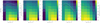 |
Fig. B.1 Same as Fig. 9 but for a UV radiation field of 10χ0. |
| In the text | |
 |
Fig. B.2 Same as Fig. 10 but for a UV radiation field of 10χ0. |
| In the text | |
Current usage metrics show cumulative count of Article Views (full-text article views including HTML views, PDF and ePub downloads, according to the available data) and Abstracts Views on Vision4Press platform.
Data correspond to usage on the plateform after 2015. The current usage metrics is available 48-96 hours after online publication and is updated daily on week days.
Initial download of the metrics may take a while.