| Issue |
A&A
Volume 696, April 2025
|
|
|---|---|---|
| Article Number | A30 | |
| Number of page(s) | 18 | |
| Section | Extragalactic astronomy | |
| DOI | https://doi.org/10.1051/0004-6361/202453292 | |
| Published online | 28 March 2025 | |
Spectroscopic active galactic nucleus survey at z ∼ 2 with NTT/SOFI for GRAVITY+ observations
1
Max Planck Institute for Extraterrestrial Physics (MPE), Giessenbachstr. 1, 85748 Garching, Germany
2
Department of Astrophysical & Planetary Sciences, JILA, University of Colorado, Duane Physics Bldg., 2000 Colorado Ave, Boulder, CO, 80309
US
3
Leiden University, 2311 EZ Leiden, The Netherlands
4
Department of Physics, Technical University of Munich, 85748 Garching, Germany
5
Departments of Physics and Astronomy, Le Conte Hall, University of California, Berkeley, CA, 94720
USA
6
Department of Physics & Astronomy, The University of British Columbia, Vancouver, BC, V6T 1Z1
Canada
7
Kavli Institute for Astronomy and Astrophysics, Peking University, Beijing, 100871
People’s Republic of China
⋆ Corresponding author; dsantos@mpe.mpg.de
Received:
4
December
2024
Accepted:
2
March
2025
With the advent of GRAVITY+, the upgrade to the beam combiner GRAVITY at the Very Large Telescope Interferometer (VLTI), fainter and higher redshift active galactic nuclei (AGNs) are becoming observable, opening an unprecedented opportunity to further our understanding of the cosmic coevolution of supermassive black holes and their host galaxies. To identify an initial sample of high-redshift type 1 AGNs that can be observed with GRAVITY+, we have obtained spectroscopic data with NTT/SOFI of the most promising candidates. Our goal is to measure their broad line region (BLR) fluxes and assess their physical geometries by analysing the spectral profiles of their Balmer lines. We present 29 z ∼ 2 targets with strong Hα emission in the K band. Their line profiles are strongly non-Gaussian, with a narrow core and broad wings. This can be explained as a combination of rotation and turbulence contributing to the total profile or two physically distinct inner and outer regions. We found small Hα virial factors, which we attributed to the low full-width-half-maximum (FWHM)/σ ratios of their non-Gaussian profiles, noting that this can lead to discrepancies in black hole masses derived from scaling relations. We also find two targets that show tentative evidence of BLRs dominated by radial motions. Lastly, we estimated the expected differential phase signals that will be seen with GRAVITY+, which will provide guidance for the observing strategy that will be adopted.
Key words: techniques: interferometric / galaxies: active / galaxies: nuclei / quasars: supermassive black holes / galaxies: Seyfert
© The Authors 2025
 Open Access article, published by EDP Sciences, under the terms of the Creative Commons Attribution License (https://creativecommons.org/licenses/by/4.0), which permits unrestricted use, distribution, and reproduction in any medium, provided the original work is properly cited.
This article is published in open access under the Subscribe to Open model.
Open Access funding provided by Max Planck Society.
1. Introduction
Supermassive black holes (SMBHs) comprise the largest black holes (BHs) in the Universe, with masses of the order of thousands to billions of solar masses. These BHs are believed to reside in the centre of galaxies and impact galaxy evolution through feedback mechanisms that regulate star formation and galaxy growth (Silk 2013; Terrazas et al. 2017; Harrison 2017). The growth of the host galaxy is also believed to affect the development of the central SMBH (Di Matteo et al. 2005; Ferrarese & Ford 2005; Peterson 2008; Gültekin et al. 2009; Yesuf & Ho 2020). This almost symbiotic relationship between the central BH and its host galaxy is reflected in scaling relationships between the BH mass and central stellar properties of the host galaxy (Kormendy & Ho 2013; Ferrarese & Merritt 2000; Marsden et al. 2020; Martín-Navarro et al. 2020). These findings invoke a coevolution scenario between the central BH and its host galaxy (Heckman & Best 2014).
Measuring SMBH masses is crucial to illuminating this scenario. In addition, measuring SMBH masses dynamically is essential to understand if and how the scaling relations typically used to infer those masses (Dalla Bontá et al. 2020; Shen & Liu 2012; Prieto et al. 2022) evolve with redshift. This is particularly important in early cosmic times when direct SMBH measurements are scarce. Most SMBH mass measurements are done via spatially resolved stellar (Saglia et al. 2016) or gas kinematics (Boizelle et al. 2019; Osorno et al. 2023), megamaser kinematics (Greene et al. 2010; Kuo et al. 2020), and reverberation mapping (RM) (Peterson 1993; Peterson et al. 2004; Li et al. 2023). However, these methods are predominantly used to probe SMBH masses of low redshift targets. Notably, performing RM at high redshifts requires long (multi-year) campaigns due to the cosmological time dilation and also because the targeted quasars (QSOs) tend to be luminous and thus have large broad line regions (BLRs) and, therefore, high SMBH masses. A recent summary of such efforts is given by Kaspi et al. (2021).
Although several observational studies have already investigated the coevolution scenario at higher redshifts (Lapi et al. 2014; Carraro et al. 2020), these works used SMBH masses derived from scaling relations and so are based on the assumption that those relations, derived at a low redshift, are also applicable at a high redshift. As such, there is a need to measure SMBH masses at a high redshift independently via direct dynamical methods.
With the unprecedented precision and resolution of GRAVITY (GRAVITY Collaboration 2017), the beam combiner at the Very Large Telescope Interferometer (VLTI), spatially resolving the BLR kinematics to measure SMBH masses has become possible in the local Universe (GRAVITY Collaboration 2018, 2020, 2021a, 2024) with very long baseline interferometry (Eisenhauer et al. 2023). Extending this endeavour to higher redshifts was one of the imperatives for upgrading GRAVITY. The GRAVITY+ project aims to add wide-field off-axis fringe tracking (called GRAVITY-Wide) and new adaptive optics systems with laser guide stars (LGSs) on all the unit telescopes (UTs). This will enable observations of both fainter and high-redshift quasars (GRAVITY+ Collaboration 2022). A key epoch to focus on is the cosmic noon in the redshift range 1 < z < 3, corresponding to about 8–12 billion years ago when star formation and BH growth both peaked (Madau & Dickinson 2014; Tacconi et al. 2020). Abuter et al. (2024) recently performed the first dynamical mass measurement of a z ∼ 2 QSO with GRAVITY-Wide. With the other improvements from GRAVITY+, a vastly wider sky coverage will open up the possibility of selecting larger samples of active galactic nuclei (AGNs) and measuring their SMBH masses. To prepare for this, we undertook a preparatory near-infrared (NIR) spectroscopic survey of promising AGN candidates for GRAVITY+. This program aims to confirm suitable targets as QSOs based on their K band Hα line profiles and fluxes. We identified the best targets for high-priority follow-up observations with GRAVITY+ by fitting their line profiles with a BLR model and estimating their expected interferometric signals. This also yields information about their BLR geometries, giving us a first glimpse of what we can learn from their BLR structure. We present 29 high-redshift targets (z ∼ 2) observed in this initial survey. For our analyses, we adopted a Lambda cold dark matter (ΛCDM) cosmology with Ωm = 0.308, ΩΛ = 0.692, and H0 = 67.8 km s−1 Mpc−1 (Planck Collaboration XIII 2016). We describe our sample selection and observations in Sect. 2. We discuss our data reduction methods in Sect. 3. We summarise the emission line properties of our targets in Sect. 4. We discuss the BLR model used for this study, our fitting methodology and results in Sect. 5. We present the estimated differential phase signals of our targets based on our BLR model fitting in Sect. 6. Finally, we present our conclusions in Sect. 7.
2. Targets and observations
The targets were selected from the Million Quasar (Milliquas) catalogue (Flesch 2021) version 7.5 (updated last 30th Apr. 2022), which provides a catalogue of type 1 QSOs and AGNs complete from literature, as well as from the Quaia spectroscopic catalogue (Storey-Fisher et al. 2024) that is based on Gaia candidates with unWISE infrared data. Our selections of type 1 QSOs required (i) 2.1 ≲z ≲ 2.6 so that Hα is redshifted into the K band, (ii) enabling GRAVITY+ observations either on-axis (i.e., K < 13) or off-axis (i.e., K < 16 as well as with a K < 13 star within 20″), and (iii) an initial prediction of the differential phase signal > 0.3° to ensure that the integration times with GRAVITY+ would be reasonable. The differential phase is an interferometric observable that measures the centroid position as a function of wavelength (see Sect. 6 and GRAVITY Collaboration 2020 for more details). The expected differential phase signal was estimated by assuming all targets lie on the Bentz et al. (2013) R–L relation. The 5100 Å luminosity was estimated by scaling the mid-IR luminosity (Krawczyk et al. 2013) SED to the observed GaiaGRP magnitude. The phase signal was then calculated using Δϕ = [f/(f+1)]RB where f is the typical line-to-continuum ratio of 3 for Hα, R is the BLR radius (in radians), and B is the projected baseline length of 100 m for the VLTI divided by the wavelength. To make an initial assessment of the properties of the selected quasars, we also looked into the archival data, particularly within the Sloan Digital Sky Survey (SDSS) Data Release 16 Quasar Catalogue (DR16Q; Lyke et al. 2020) and the UV Bright Quasar Survey Catalogue (UVQS; Monroe et al. 2016) for their optical and ultraviolet (UV) spectra, respectively, to confirm AGN features such as the blue continuum and broad C IV, Mg II, or Lyα lines.
After the sample selection, 72 observable unique targets were selected. Observations were performed between April 2022 and February 2023 with the infrared spectrograph Son of ISAAC (SOFI) at the 3.6-m New Technology Telescope (NTT), which is operated by the European Southern Observatory (ESO). Due to weather conditions, we were able to observe 49 targets with NTT/SOFI. Since our goal is to pick objects that are suitable for GRAVITY+ observations, we only analysed those with sufficiently strong Hα lines (i.e. integrated flux ≳5 × 10⁻¹⁶ erg s−1 cm−2). We then narrowed our sample to 29 targets. Some of the faint targets have signal-to-noise ratio (S/N) values between 4 and 10, while the brightest targets have S/N as high as 40–55. Table A.1 lists the 29 targets with good spectra, which are analysed for this study, together with a summary of their observations, which include the date of observation, exposure time, airmass, seeing, and S/N.
The initial two runs were performed using medium resolution spectroscopy with the Ks filter (2.00–2.30 μm, grism no. 3 with R ∼ 2200, with a dispersion of 4.62 Å pixel−1) and a 1″ slit. For the remainder of the runs, we switched to the low-resolution spectroscopy with the GRF filter (1.53–2.52 μm, red grism with R ∼ 980 with a dispersion of 10.22 Å pixel−1) and a 0.6″ slit due to the wider wavelength range it provides, allowing better constraint on the continuum and possible detection of Hβ and Hγ lines compared with the Ks filter. The K-mag values and exposure time of each target are presented in Table A.1. For the science observations, we used the auto-nod non-destructive readout mode of SOFI provided by the SOFI_spec_obs_AutoNodNonDestr template. A telluric star was observed after each AGN observation to enable atmospheric correction and flux calibration. For the spectral calibration and flat fielding, we took xenon and neon arc lamp observations and dome flat exposures before the start of each night. These observations were taken with the SOFI_spec_cal_Arcs and SOFI_spec_cal_DomeFlatsNonDestr observation templates, respectively, using the same slit and filter as our observations for the night.
3. Data reduction
The data were reduced with version 1.5.0 of the SOFI pipeline. The flat fields and arc frames were processed using the sofi_spc_flat and sofi_spc_arc recipes, respectively. For low-resolution data, we had difficulties obtaining a dispersion solution that matched the H and K bands simultaneously. We, therefore, applied a quadratic correction to each band separately, based on the atmospheric OH lines in the H band and on the arc lines in the K band. The science data were processed using sofi_spc_jitter recipe to produce a 2D spectrum. Although this recipe can combine the individual frames and extract a final 1D spectrum, we used our own algorithms for these steps. Each 2D spectrum was trimmed in the spatial direction, and then a line-by-line residual background was fitted away from the object trace and subtracted. The frames were aligned to integer pixel precision based on the spectrally summed trace and then combined while rejecting deviant values. A final iteration of the line-by-line subtraction of the median in each row was then performed on the combined frame. From this 2D product, we extracted a 1D spectrum on which we performed telluric correction and flux calibration.
The spectral extraction was based on the optimal extraction method described by Horne (1986), with some adaptations to match it to the pipeline process and the data properties. A description of the implementation is given in the Enhanced Resolution Imager and Spectrograph (ERIS)-SPIFFIER Pipeline Manual1. This method is suitable for sources where the spatial distribution changes only gradually with wavelength, including unresolved sources such as stars and the QSOs in our sample. The routine begins by defining a region around the spectral trace that encompasses all the flux. This defines the source values Dxλ as a function of spatial location x and wavelength λ, and the variance values Vxλ as the square of the noise. An initial spectrum is created as fλinitial = ΣxDxλ with variance var[fλ] = ΣxVxλ. A model of the spatial distribution of the source (or point spread function/PSF) Pxλ is then constructed by normalising each spectral slice so that Pxλ = Dxλ/fλ. The resulting model Pxλ is essentially the probability that a detected photon with wavelength λ falls on pixel x. Because Pxλ is by definition strictly positive, in the first step, any negative values of Pxλ are set to zero. The second step is to provide some regularisation along the spectral direction, so at each spatial location x, the spectral values of Pxλ are traced. Rather than fit these with low-order polynomials as was done by Horne (1986), we applied a running median filter. In both cases, the same purpose is achieved: to reject outliers, which is the second core part of the algorithm. Any pixel in Pxλ for which (Dxλ − fλPxλ)2 > σclip2V is set to zero. The threshold σclip is derived using a percentile clipping of the values and is calculated for each spectral row to allow for strong variations in the S/N along the spectrum. The spectrum estimator is then defined to be a linear combination of unbiased pixel estimates such that
where the variance of the weighted mean is minimised by choosing weights that are inversely proportional to the variance of the variables, so that
![$$ 1/W_{x\lambda } = var[D_{x\lambda } / P_{x\lambda }] = V_{x\lambda } / P_{x\lambda }^2. $$](/articles/aa/full_html/2025/04/aa53292-24/aa53292-24-eq2.gif)
Substituting these weights into the equation above, one can find the optimal extraction of the spectrum f such that when it is multiplied by the source model P, the result matches the data D, which has variance V. The initial optimal spectrum can then be expressed as
with variance
![$$ var\left[f_\lambda ^\mathrm{optimal}\right] = \frac{1}{\Sigma _x \left(P_{x\lambda }^2 / V_{x\lambda }\right)}\cdot $$](/articles/aa/full_html/2025/04/aa53292-24/aa53292-24-eq4.gif)
This process is then iterated a second time replacing the initial estimate of fλ with the first estimate of the optimised spectrum, to yield the final estimate of the optimised spectrum.
The telluric star was used both to correct the atmospheric absorption and for flux calibration. The former was achieved by modelling the star (spectral type B) as a blackbody with Brγ absorption and normalising the resulting telluric spectrum to a maximum value of 1. The flux calibration was performed by taking the ratio of the counts within 2.0–2.3 μm and the expected K band flux calculated from the magnitude. We compare the measured Kmag values of our targets based on their average flux densities with the Kmag values from their catalogues, and find that our targets are ∼0.44 mag fainter than expected. This translates to a ∼33% lower detected flux than expected. We discuss the possible cause of such lower measurement in Sect. 4.4.
4. Emission line properties
This section focusses on the observed properties of the emission lines. We first applied a line decomposition in order to separate the broad component from other features in the spectrum. We then assessed the properties of the broad line emission, in particular, the full-width-half-maximum (FWHM) to σ ratios and the Hα/Hβ flux ratios of our targets.
4.1. Line decomposition
In this Section, we describe the fitting of the Hα, Hβ, Hγ, and [O III] lines as well as the continuum and iron complex (noting that for the medium resolution data taken with the Ks band filter, only the Hα line is covered). We used the SAGAN code2 to decompose the spectra.
The Hα lines were fitted with two Gaussian components when there was a clear superposition of a narrower core (that is much broader than the typical width of a narrow-line component expected from the narrow-line region or NLR) and a broader wing component. We impose criteria to determine whether the double Gaussian model is a better fit than the single Gaussian model. Once all criteria are met, the double Gaussian model is preferred. Otherwise, we follow the single Gaussian model fit. Our criteria are similar to that of Oh et al. (2024):
-
The reduced chi-square value of the double Gaussian fitting is less than that of the single Gaussian fitting (χD2 < χS2), where D and S refer to double and single Gaussian model, respectively;
-
The S/N of the wing and core components should be greater than 3;
-
The wing component flux contributes to 10–90 percent of the total flux fW/(fW + fC) where W and C refer to the wing and core components, respectively); and
-
The velocity dispersion of the broad component should be greater than that of the narrow component by at least its uncertainty (σW − σW, err > σC).
With these criteria, we were able to confidently choose 21/29 Hα lines to be fitted with the double Gaussian model, and the rest were fitted with the single Gaussian model. We also note that most of the emission lines fitted with the single Gaussian model have S/N ≲8. For the Hβ and Hγ lines, we fit them with the same line profile as the Hα line. If the double-Gaussian model is used, the velocity shift difference between the two Gaussian components is also fixed when fitting the other Balmer lines. We do not assume a theoretical flux ratio of fHα/fHβ = 3–3.5 as shown by previous works (Dong et al. 2008; La Mura et al. 2007) as it fails to produce a meaningful fit, which tells us that our targets do not exhibit such a flux ratio. We found three targets that are exempted from our usual line decomposition method: ID#23, which shows a relatively large deviation between the Hα and Hβ velocity shifts (∼1500 km/s) despite being fitted with a similarly shaped Gaussian component; ID#25, which shows Hβ to be fitted with one Gaussian component while its Hα line is fitted with two Gaussian components; and ID#29, where Hβ is much wider than the Hα line. Tables A.2 and A.3 show the line-fitting results of Hα, Hβ, [O III], and Hγ lines, while Table A.4 shows the line-fitting results of the three Hβ lines that did not have the same line profile as their Hα lines. We also used the central wavelength of the Hα line to verify or update the redshift of each target taken from the source catalogues.
Balmer lines are usually composed of the broad component originating from the BLR, and the narrow component originating from the NLR. Most works use the [S II] doublet as the narrow line template, but in the case that it is not observable, the [O III] doublet can be used (Greene & Ho 2004). However, the [O III] doublet suffers from possible contamination of outflowing components, which could indicate a dynamic NLR (Whittle 1985; Boroson 2005; Marziani et al. 2017), making it a less suitable narrow-line template. To check whether we need to fit the narrow component with a template, we first chose targets with observable [O III] doublet, that is, the S/N of [O III] > 3 and the doublet is not obscured by any atmospheric feature. Seven targets were selected using these criteria. Their Balmer lines were then fitted with the single/double Gaussian model (whichever is suited based on the aforementioned criteria) plus the narrow component with a similar line width as the [O III] doublet. Afterwards, we measured the narrow components’ flux contribution to the fitted Balmer lines. Only three targets (ID #9, 10, and 17) showed a > 5% flux contribution of the narrow components on their Balmer lines. We also did not find any drastic change in our results (i.e. best-fit BLR parameters and virial factor; see Sects. 5.2 and 5.3) and conclusions after removing the fitted narrow components from the Balmer lines of these three targets. Hence, we decided not to include any narrow component fitting in all of our targets.
In most cases, the continuum, which was fit together with the rest of the emission lines, was represented with a power law. However, in a few cases where the power law continuum does not give a good fit (6/29 targets), a 4-degree polynomial was used instead. The polynomial degree was chosen as it is the smallest degree that provides a converging result for these exceptional cases. For these objects fitted with a 4-degree polynomial as their continuum, there is sufficient wavelength range outside the broad line emission. An iron template based on I Zw 1 (Park et al. 2022) was included in the fit when there were clear Fe II features around the Hβ and [O III] lines. Fig. 1 shows example results of the line decomposition for three targets with different properties: (a) a target observed with the GRF filter which has strong Fe II features but noisy [O III] lines due to atmospheric absorption (hence it was not chosen for fitting the narrow component with the [O III] doublet as a template), (b) a target observed with the GRF filter with slightly asymmetric Hα, no Fe II features, very strong [O III] lines and significant narrow components in their Balmer lines, and (c) a target observed with the Ks filter with a strongly asymmetric Hα line that has a bump on the redshifted side of the Hα central wavelength (and which is discussed in Sect. 4.2).
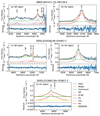 |
Fig. 1. Representative line decomposition results for three of our SOFI z ∼ 2 targets. Each row refers to a different target (QBQS J051411.75-190139.4, SDSS J220245.60-024407.1, and SDSS J121843.39+153617.2), while each column refers to a different spectral region (Hβ and Hα). The observed data are shown in blue, while the cumulative best-fit spectrum is shown as an orange solid line. The different coloured lines pertain to different components in the line decomposition, as shown in the legend. Some of our targets have strong Fe II and even clear Hγ emission, as shown in the Hβ region of QBQS J051411.75-190139.4 (panel a). On the other hand, a few targets have prominent (S/N > 3) [O III] features similar to SDSS J220245.60-024407.1 (panel c). Both of these objects were observed with the GRF filter, hence other Balmer lines aside from Hα are detected. On the other hand, SDSS J121843.39+153617.2 was observed with the Ks filter (panel e). Its Hα spectrum shows a weak [N II] λ6584 feature (see Sect. 4.2). |
The uncertainty in the flux density for all spectral channels was calculated as the standard deviation of the fitting residual. From the decomposition, we measure the line fluxes and luminosities, their FWHM values, and also the dispersions σ defined as the square root of the second moment of the line (Dalla Bontá et al. 2020). Both the FWHM and σ are calculated from the best-fit line and are corrected for instrumental broadening. The 1σ uncertainties of these quantities are derived using Monte Carlo techniques, perturbing the spectrum 1000 times with the uncertainty in the flux density. We normalise the Balmer lines by the continuum for BLR fitting (see Sect. 5.2).
4.2. Line properties of the z ∼ 2 targets
Among the 29 targets, 24 have data covering both H and K bands. Of those, 17 have significant Hβ emission, and two also have observable Hγ emission. It is important to bear in mind the number of Gaussian components used to fit the Balmer lines. Most of the Balmer emission lines are fitted with two Gaussian components comprising a narrower core component (with σ ≲ 1200 km s−1) and a broad wing component (typically with 1500 ≲ σ ≲ 3000 km −1).
The corrected redshifts of our targets are almost all consistent within their 1σ uncertainties with the redshifts from their respective catalogues, as expected. For 10 of the 17 targets with Hβ emission lines, the [O III] doublet has been detected and fitted as well, similarly to SDSS J220245.60-024407.1 (ID#15). Five of these have σ ≳ 1000 km s−1 for the [O III] lines. In addition, six targets have clear Fe II signatures in their spectra. We do not investigate these lines or Hγ further, and instead, we focus our analysis on the stronger Balmer lines Hα and Hβ.
As noted previously, one particular target, ID#1 (SDSS J121843.39+153617.2), has a bump on the redshifted side of the Hα peak (see Fig. 1). Its wavelength corresponds to a velocity offset of ∼2300 km s−1 with respect to Hα, but only ∼1450 km s−1 with respect to [N II] λ6584. Although [N II] is a doublet, the other line [N II] λ6548 is a factor 3 fainter (Acker et al. 1989) and so a corresponding feature would not be detectable. In addition, the calculated velocity offsets should not be taken too seriously due to the uncertainty of the redshift taken from the original catalogue, which is σz ∼ 0.01, which translates to ∼3000 km/s (Onken et al. 2023). We therefore consider the bump to be associated with [N II] λ6548 due to the lower velocity offset. We note, however, that the results of our analyses for this target do not change even if the bump is considered as another Hα component. We also do not have any other narrow line present in our spectrum of this target to calculate the redshift.
4.3. FWHM versus σ and the BLR model
One of the most important properties of the line emission in terms of BLR modelling is the shape of the line profile. A simple way to quantify this is via the ratio of FWHM to σ, which has been shown to be a good measurement of line shape because FWHM is core sensitive while σ is wing sensitive (Wang et al. 2019). We plot the line shape, quantified in this way, as a function of FWHM in Fig. 2 for the Hα lines. We focussed on the Hα lines fitted with the double-Gaussian model, as the targets fitted with the single-Gaussian model will lie at the Gaussian limit (i.e., FWHM/σ = 2.35) shown as a horizontal line, and we found systematic uncertainty in the Hβ lines (see Sect. 4.4). Compared with the theoretical line width ratios from Kollatschny & Zetzl (2011) and Kollatschny & Zetzl (2013) (as shown by the black and grey dashed lines), our line width ratios are smaller but show a similar trend as their work and Wang et al. (2019): that the FWHM/σ increases with FWHM. Targets with low FWHM and FWHM/σ have line profiles that more closely resemble a Lorentzian profile: a superposition of a very broad component and a strong, more prominent core. On the other hand, targets with high FWHM and FWHM/σ have line profiles that more closely resemble a Gaussian profile; indeed, at much higher FWHM values, the trend asymptotically reaches the Gaussian limit. Comparing our sample with the low redshift work of Villafaña et al. (2023), Kollatschny & Zetzl (2011), and Kollatschny & Zetzl (2013), we found no significant difference (Pearson correlation p-value ≫ 0.05) in the distribution of line shape versus FWHM between our sample and their AGN samples.
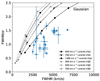 |
Fig. 2. Ratio of FWHM to σ (line shape) of Hα lines fitted with the double-Gaussian model as a function of FWHM. The Gaussian limit (FWHM ∼ 2.35σ) is shown as a horizontal grey solid line. The error bars denote 1σ uncertainties. For comparison, we plot the theoretical line width ratios of rotational line broadened Lorentzian profiles for Hα (black dashed lines and markers) and Hβ (grey dashed lines and markers) which were taken from Kollatschny & Zetzl (2011) and Kollatschny & Zetzl (2013). Different markers pertain to different FWHMs of the Lorentzian profiles. |
We discuss below two explanations for such profiles. The first scenario, a two-component BLR, would tend to favour fitting the profile with two distinct components. The second scenario, which explains the profile as a combination of turbulence and rotation, would tend to favour fitting the line with a Voigt profile that is a convolution of a Lorentzian profile with a Gaussian. While we have chosen to fit the profiles with two Gaussians, this is done for the convenience of quantifying σ, and does not imply a preference for one explanation over the other.
4.3.1. Scenario 1: Two-component BLR model
A two-component BLR has been discussed extensively in the literature (e.g. Brotherton et al. 1994; Popović et al. 2004; Zhu et al. 2009; Zhang 2011; Ludwig et al. 2012; Nagoshi et al. 2024). In this scenario, the BLR is composed of two components. The first one is an inner disc – the very broad line region (VBLR) – that is more closely associated with the accretion disc and is responsible for the broad wings of the observed emission line. Zhu et al. (2009) suggests that the VBLR represents the “traditional” picture of the one-component BLR and is the region responsible for the observed ∼0.5 slope in the size-luminosity relation. Indeed, there have been recent claims for detecting Keplerian rotation in this inner disc from the variability of its micro-lensing response (Fian et al. 2024). The second component is an outer and more spherical part – the intermediate line region (ILR) – which produces the narrow core of the profile. The ILR, which is situated at a larger distance from the ionising source, is thought to have higher gas density and be flatter than the VBLR; and is suggested to represent the inner boundary layer between the BLR and the dusty torus of the AGN. It has been argued that such BLRs with two components occur both in the low-redshift (Zhu et al. 2009) and high-redshift (Brotherton et al. 1994) Universe. Zhang (2011) argued that the ILR of the reverberation-mapped AGN PG 0052+251 was strongly obscured because, in contrast to its Hα line, its Hβ line profile does show a clear core component in the line decomposition. While we consider this result uncertain because of the low quality of the spectrum in the Hβ line region of their source, such an explanation could, in principle, apply to the different line widths of Hα and Hβ of ID#15 that was shown in Sect. 4.2. Storchi-Bergmann et al. (2017) also finds that aside from the ubiquity of a disc component in most BLRs, an additional line-emitting component arises at higher Eddington ratios and higher luminosities for Seyfert 1 galaxies. This component is reminiscent of the ILR component, and, as suggested by Storchi-Bergmann et al. (2017), may be inflowing (Grier et al. 2013), outflowing (Elitzur et al. 2014), or simply have more elliptical orbits (Pancoast et al. 2014).
The limitation of this explanation is that there is no clear reason why, when considering these two components together, there should be a relation between FWHM and FWHM/σ as seen in Fig. 2. Collin et al. (2006) proposed that this distribution may be associated with the Eddington ratio and, hence, the accretion rate. They suggested that at large radii, where the self-gravity of the disc overcomes the vertical component of the central gravity due to the SMBH, the resulting cloud collisions due to the gravitational instability would heat the disc and increase its turbulence. And, based on a correlation between the ratio of the BLR size to this radius and the Eddington ratio, these authors speculated that gravitational instability may be stronger in AGN with higher Eddington ratios, leading to greater turbulence, which perhaps constitutes the start of a disc wind. This results in a very broad component in the line profile, as exhibited by the low FWHM/σ (i.e. low FWHM) sources. On the other hand, weaker accretion produces a more stable BLR, producing Gaussian-like line profiles.
4.3.2. Scenario 2: Presence of turbulence and rotation
This relation is specifically addressed in the phenomenological approach put forward by Kollatschny & Zetzl (2011). For a disky BLR, the ratio between the turbulent and rotational velocity is proportional to the ratio between the height and radius of the BLR. Since the rotational velocity is found to increase with increasing FWHM (Kollatschny & Zetzl 2013), objects with high FWHM and, therefore, high FWHM/σ have a fast-rotating geometrically thick and flat BLR. In contrast, objects with low FWHM and, therefore, low FWHM/σ have slow-rotating spherical BLRs. These authors noted that while the Balmer lines tend to originate at moderate distances above the disc plane, the highly ionised lines come from smaller radii and at greater scale height and that the resulting geometries resembled disc winds models. Thus, without explicitly requiring two distinct components, an understanding of the geometry and kinematics of the BLR does lead to insights into the various physical processes occurring in this region. This perspective matches the approach we adopt when modelling the BLR (see Sect. 5). We fit the line profile (and differential phase data from GRAVITY/+ when available) with a single model that encompasses both rotation and dispersion without physically separating them. The dispersion comes directly from the geometry in terms of the thickness, or opening angle, of the BLR and the distribution of clouds within it. It is also affected by whether there is a radial component, whether inflowing or outflow. Thus, here, too, there is a continuous distribution of potential models from a thin rotating disc through a turbulent, thick rotating disc to a combination of rotation and outflow.
The interpretations above seem likely to be different perspectives on the same underlying processes and geometries that invoke a rotating (thick) disc together with a region or component of that disc where the gas has increased turbulence and scale height, and so may be the origin of the expected disc wind. However, there is a major difference between them that needs to be resolved. The wings of the profile trace the rapidly rotating inner disc in the two-component scenario, while they trace the turbulence in the Voigt profile interpretation. Similarly, the core of the profile traces the outer, more spherical distribution in the two-component model while it traces the rotation in the Voigt profile. This aspect needs clarification if we are to fully understand the BLR.
4.4. Luminosity ratio (Balmer decrement)
As discussed in the previous section, the Hα lines are mostly fitted with two Gaussians, while the Hβ and Hγ lines are fitted with the same line profiles as their respective Hα lines with the exception of three targets. To further assess the properties of our targets, we investigate the ratio between Hα luminosity and Hβ luminosity (i.e. the Balmer decrement) as a function of Hα luminosity.
Fig. 3 shows the Balmer decrement as a function of Hα luminosity. The Balmer decrement does not show a significant correlation with LHα (the probability of it occurring by chance is p = 0.101 or 1.3σ), although it seems to exhibit a positive correlation (correlation coefficient ρ = 0.41) similar to previous works (e.g. Domínguez et al. 2013; Reddy et al. 2015). Furthermore, the Balmer decrements of our targets are > 3.5. The large Balmer decrements suggest that we are missing a significant fraction of the Hβ luminosity and therefore, there is a systematic uncertainty associated with the Hβ emission lines that go beyond the nominal statistical uncertainty derived from the fits. This is due to the limitation of the data rather than having a physical cause, and caution is needed when interpreting values related to Hβ, especially the size of the Hβ-emitting region of the BLR.
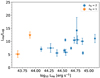 |
Fig. 3. Ratio between Hα and Hβ luminosity as a function of Hα luminosity. The blue (orange) points show the targets that are fitted with a double (single) Gaussian model. We remove two targets (from the three exceptions in Table A.4) whose Hβ lines cannot be fitted with the same number of Gaussian components and line shape as that of Hα. The error bars are 1σ uncertainties. |
It is possible that such large Balmer decrements could be due to significant contributions from Wolf-Rayet or late-type OB stars (e.g. Crowther & Bohannan 1997). However, this reason is unlikely to be the cause of the observed Balmer decrements in our sample since these targets are quasar-dominated as per our check of archival spectral data from SDSS DR16Q and UVQS catalogues. The Balmer decrements of our sample are higher than one would expect from typical star-forming galaxies (SFGs) at z ∼ 2, which are also found to increase with stellar mass and (Shapley et al. 2022; Maheson et al. 2024). Considering also that we found higher Hα/Hβ ratios than the expected value of ∼3.1 (Dong et al. 2008; La Mura et al. 2007), these suggest that dust extinction might cause such large Balmer decrements in our sample. To confirm whether dust extinction is the cause of such large Hα/Hβ ratios in our sample, we estimate the typical extinction coefficient (AV) of our sample based on our median Hα/Hβ value of ∼7.45. Using Eqs. (4) and (7) of Domínguez et al. (2013), we found AV ∼ 3 which translates to a column density of NH ∼ 6 × 1021 cm−2. These values are larger than most SFGs at high-z, but still within the acceptable range of AV values for Type 1–1.5 AGNs (Burtscher et al. 2016). However, such large AV should also lead to obscuration of the BLR light, which is not the case for our targets. In addition, an extinction coefficient of AV ∼3 translates to a detected flux that is ∼10% of the intrinsic flux. However, based on our comparison between our measured and expected Kmag values in Sect. 3, we found that we are detecting (on average) ∼33% of the intrinsic flux of our sample. Therefore, we cannot conclude with confidence that dust extinction is the root cause of our observed large Balmer decrements.
Nevertheless, other alternative explanations for the large Balmer decrements of AGNs have also been put forward, such as the intrinsic property of the BLR, that is, the BLR consists of clouds with low optical depths and low ionisation parameters (Kwan & Krolik 1981; Canfield & Puetter 1981; Goodrich 1990), or the possible role of accretion rate (Wu et al. 2023). Although we cannot confirm the cause of the large Balmer decrements in our sample, we expect that these should only affect the estimated single-epoch BH masses, BLR radii, and expected differential phase signals of our targets, which are all dependent on the Hα luminosity, but not the geometry and virial factors based on our BLR fitting results (see Sect. 5).
4.5. BH mass and bolometric luminosity estimation
Two of the important parameters we need for comparison with future GRAVITY+ observations of z ∼ 2 are SMBH mass (MBH) and bolometric luminosity (Lbol) estimates. We present the first estimates of MBH and Lbol in columns 7 and 8 of Table A.2. We present the parameter space that we are probing with our SOFI z ∼ 2 targets in Fig. 4. For comparison, we also show the low-luminosity z ∼ 2 AGNs from Suh et al. (2020) and the high-luminosity z ∼ 2 AGNs from the WISSH survey (Bischetti et al. 2021).
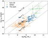 |
Fig. 4. Logarithm of bolometric luminosity as a function of the logarithm of BH mass. For the SOFI z ∼ 2 targets (This work, blue data points), the Lbol are estimated from Hα, while the MBH are estimated using Eq. (6) of Woo et al. (2015) which uses the dispersion (σ) and Hα luminosity as inputs. The typical error of log Lbol is shown as the blue vertical error bar on the lower right of the panel. For comparison, we show the sample of z = 1.5–2.5 with Lbol < 47 as orange points (Suh et al. 2020) and high-luminosity quasars from the WISSH survey as green points (Bischetti et al. 2021). The grey dashed lines pertain to the loci of the same Eddington ratio: λEdd = 0.01, 0.1, 1, and 10. For the WISSH quasars, we assume a BH mass uncertainty of ∼0.47 dex following the prescription for the 1σ relative uncertainty of single-epoch BH mass estimates from Vestergaard & Peterson (2006). However, we do not include the systematic uncertainties for the absolute calibration of RM masses. |
In their Eqs. (5) and (6), Woo et al. (2015) calculated the SMBH mass as a function of Hα luminosity and either FWHM or σ. These have different values of the virial factor: for σ, f = 4.47, while for FWHM, f = 1.12. The resulting SMBH masses of our targets from these equations are consistent with those derived from relations presented elsewhere (e.g., Dalla Bontá et al. 2020). While there are advantages and disadvantages of different line width measurements for calculating SMBH masses (Peterson et al. 2004; Wang et al. 2020), we report the σ-calculated single-epoch BH mass estimates because it has been argued to have a tighter virial relationship than FWHM (Peterson et al. 2004), and FWHM can lead to overestimation at higher SMBH mass and underestimation at lower mass (Dalla Bontá et al. 2020). Because not all targets were observed in the necessary band, the λLλ(5100 Å) continuum luminosities are instead calculated using Eq. (4) of Woo et al. (2015) from the Hα luminosity, and the uncertainties are derived by calculating the distribution of SMBH masses via Monte Carlo method, assuming Gaussian distributions of the virial factor f, Hα luminosities and σ values. To convert the λLλ(5100 Å) to Lbol, we used the bolometric correction formula from Trakhtenbrot et al. (2017) which is similar to the bolometric correction of Suh et al. (2020) and Bischetti et al. (2021). We see that our SOFI z ∼ 2 AGNs are located between the two AGN samples, particularly at moderate BH masses (log MBH ∼ 8 − 10.5) and bolometric luminosities (log Lbol ∼ 45 − 47), which translates to moderate accretion rates (Eddington rates of λEdd ∼ 0.1).
5. BLR modelling
Following the assessment of the line profiles, we fitted them with a BLR model. In the following subsections, we describe the model used and the simplifications we adopt, the general results, and implications for the virial factor. We finish by looking at two targets for which the asymmetry of the line profiles warrants a more detailed approach than the majority of the sample.
5.1. Description of the BLR model
We followed the BLR model fitting methodology introduced by Kuhn et al. (2024), which was developed based on Pancoast et al. (2014) and Stock (2018). Rather than model the distribution of BLR clouds and calculate their line emission based on photoionisation physics, we model the distribution of line emission directly. As such, the model focusses on geometry and kinematics without considering the absolute flux scaling. The model is adapted into a Python package called DyBEL which can be used to fit either a single line (only Hα) or two or more lines simultaneously (e.g. both Hα and Hβ). In this section, we briefly describe the most important parameters in the model. We highly recommend the reader to refer to Pancoast et al. (2014) and GRAVITY Collaboration (2020) for more quantitative details of the BLR parameters used in our model.
The model assumes a large number of non-interacting clouds (or “line emitting entities”, not to be confused with actual physical gas clouds) orbiting a central SMBH with mass MBH. A shifted Gamma function describes the radial distribution of the clouds. It is controlled by three parameters: the mean radius μ (in this case, the average emissivity-weighted BLR radius), the fractional inner radius F = Rmin/μ where Rmin is the minimum BLR radius, and the shape parameter β which defines the radial cloud distribution: Gaussian (0 < β < 1), exponential (β = 1), or heavy-tailed (steep) inner profile (1 < β < 2). The inclination angle, i, is the angle of the BLR relative to the plane of the sky and is defined such that a face-on geometry is i = 0°, while an edge-on geometry is i = 90°. The opening angle, θ0 describes the angular thickness of the BLR and gives the BLR model a “flared disc” shape. It is defined such that a thin disc has θ0 = 0°, while a spherical system has θ0 = 90°. It is the combination of the flared disc shape and the ellipticity of the orbits (see below) that enables our model to fit targets with a variety of FWHM/σ.
Asymmetries can also be introduced into the model. For example, the vertical distribution of the clouds is assigned by the parameter γ, which ranges from 1 to 5. The larger γ is, the more concentrated the clouds are towards the disc surface. Anisotropic emission from each cloud is parameterised by κ, which describes the weight of each cloud’s emission. The value of κ ranges from −0.5 to 0.5. If κ > 0, clouds closer to the observer (i.e. located on the near side of the BLR) have higher weights, and vice versa. Midplane obscuration is controlled by the parameter ξ, with ξ = 1 pertaining to a transparent midplane (i.e. the numbers of observable clouds on both sides of the midplane are equal), and ξ = 0 pertaining to a completely opaque midplane (i.e. the emission of the clouds below the midplane cannot be seen).
The kinematics of the clouds can include not just circular orbits but also elliptical orbits and, hence, radial motion in a way that is still governed by the gravitational potential of the SMBH. It is done with the parameter fellip, which controls the percentage of clouds in circular or bound orbits and unbound orbits that are dominated by radial motion. Each cloud has a radial (vr) and tangential (vϕ) velocity component to facilitate inflowing and outflowing clouds. A binary parameter, fflow controls the direction of the radial motion: inwards (fflow < 0.5) or outwards (fflow > 0.5). The components vr and vϕ are randomly distributed around a point on an ellipse in the vr-vϕ plane. Clouds on circular orbits, where  , are at (0, ±vcirc). Clouds dominated by radial motion possess highly elongated orbits with a maximum radial velocity equal to the escape velocity
  , and are located at the point (±vesc, 0). For these clouds, there is an extra angular parameter θe = arctan(|vϕ|/vr) which defines the angular position of the clouds around that ellipse, with θe = 0 denoting where the orbits are unbound. Lastly, there are two additional parameters which do not contribute to the BLR geometry (and are thus ‘nuisance’ parameters): the peak flux (fpeak) and central wavelength (λc) of the line. The priors of all parameters are adapted from GRAVITY Collaboration (2020).
The model described above is used to fit the line emission distribution of the BLR, excluding any photoionisation physics. Following previous work (Kuhn et al. 2024; GRAVITY Collaboration 2020, 2024; Abuter et al. 2024), we used the Python package dynesty (Speagle 2020) together with a nested sampling algorithm (Skilling 2004) to fit the data. We used 1200 live points with the dynamic nested sampler (DynamicNestedSampler) and the random walk (rwalk) sampling method. The rest of the options in dynesty were set to their default values. Following Kuhn et al. (2024), a temperature parameter T was also defined. This parameter was set to 16 in order to provide likelihood functions with fewer peaks and, hence, a better estimation of the posterior distributions. The spectrum was normalised by the continuum so that we effectively fit the line-to-continuum ratio (as a function of observed wavelength). We note that this is also used to estimate the expected differential phase signal of the target (see Sect. 6).
Using a spectrum of NGC 3783, Kuhn et al. (2024) demonstrated that fitting Hα, Hβ, Hγ, He I, and Paβ lines simultaneously provide tighter constraints on the BLR parameters of NGC 3783 than fitting them separately and that both methods provide consistent geometry with that derived from the RM and GRAVITY data (GRAVITY Collaboration 2021a,b; Bentz et al. 2021). When an object has Hβ and Hγ line profiles available, we include them in the fit after tying many of their parameters. In particular, their central wavelengths are tied so that they all shift by the same small amount ϵ = λc/λair − 1, where λc is the theoretical central wavelength of the line, and λair is the wavelength measured in air. There are two exceptions to this where, because of the wavelength calibration method described in Sect. 3, leaving ϵ untied yielded better results, and these are indicated in column 3 of Table B. In addition, while allowing the BLR radii derived from each line to be free, we tie the shape of their radial profiles using the β and F parameters. All other parameters are tied except fpeak, which we set to be free for all lines.
It should be noted that since we fit only the spectrum, RBLR and MBH are fully degenerate because the circular velocities vcirc of the clouds depend on the ratio of MBH and RBLR. Hence, one of them must be fixed during fitting. We fix MBH to the values estimated in Sect. 4.5.
Finally, for all of our targets, we try two variations of the BLR model: the full model, which fits all the asymmetry parameters (γ, κ, ξ, fflow, fellip, and θe), and the circular model, for which these are fixed to ‘neutral’ values (γ = 1, κ = 0, ξ = 1, fflow, and fellip = 1 so that θe and fflow have no impact). Our results indicate that in most cases, the resulting BLR geometry and kinematics (in particular, the best-fit values of i, θ0, and RBLR) are fairly similar for both options. However, some targets are definitely fitted better with the full model due to their asymmetric profiles (see Sect. 5.2). These can be identified in Table B by the entries for their asymmetry parameters.
5.2. BLR fitting results
In this section, we give an overview of the results from our fits, including the characteristic geometry from the ensemble of best-fit BLR models, and the typical range of values for each fitted parameter. Appendix B provides the details, listing all the values of the best-fit parameters for each target.
It is important to note that due to the fact that we are only fitting the spectra of our targets, it is inevitable that our fitting results will yield large uncertainties especially in their best-fit parameters values including those that describe the overall geometry of the BLR such as β, i, and θ0. Instead of focusing on each individual best-fit parameter values of our targets, we focus on the summed posterior distribution of the best-fit parameters to shed light on the overall behaviour of our fitting results. Therefore, we caution that the individual best-fit values should not be over-interpreted.
Fig. 5 shows the population distributions for several key BLR parameters (β, i, θ0, FHα, and μ). Their ranges reflect both the distribution and uncertainty of the individual best-fit values. The distribution for β suggests that our targets are typically fitted with a heavy-tailed (β > 1) radial distribution of BLR clouds with a significant number of line-emitting clouds at larger radii. The inclination peaking at i < 45° indicates that the BLRs are, as expected, generally viewed closer to face-on than edge-on. And the opening angle θ0 ∼ 50° suggests that they tend to have fairly thick discs. The typical Hα BLR radius spans a range from a few hundred to a few thousand light days, which encompasses the radius reported for the z = 2.3 QSO that was derived from modelling GRAVITY data (Abuter et al. 2024) This also reflects the two orders of magnitude range of SMBH mass estimates of our targets as shown in Sect. 4.5.
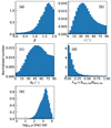 |
Fig. 5. Normalised (i.e. independently for each histogram such that the area under the histogram is 1) histograms showing in blue the summed posterior distributions of the BLR parameters from the best fits to all the z ∼ 2 targets. The panels correspond to (a) the radial distribution of BLR clouds, (b) the inclination angle, (c) the opening angle, with the minimum and maximum values defining the thin disc and spherical shape, respectively, (d) the ratio between the minimum and mean Hα BLR radius, and (e) the mean (emissivity) Hα BLR radius. |
5.3. Virial factor and its dependence on the line shape and BLR parameters
The virial factor, which is calculated as f = GMBH/(RBLRv2), does not depend on the assumed MBH value because the MBH the RBLR are degenerate (i.e. scaling together without changing the line profile) and RBLR is set as a free parameter in our BLR fitting (Kuhn et al. 2024). Hence, our fits can produce meaningful virial factors for our targets. We note that the choice of using either the circular or full BLR model does not affect the resulting virial factor. In this Section, we discuss the dependency of the virial factor on various parameters. One focus is on whether one puts v = σ or v = FWHM. Another is on i and θ0, which have been shown to greatly affect the observed line profiles (e.g., Stock 2018; Raimundo et al. 2019) In addition, Villafaña et al. (2023) investigated correlations of the virial factor with various parameters – including those above – based on 28 low redshift AGNs and dynamical modelling with the same BLR model as Pancoast et al. (2014). Using the Hβ line, they measured the virial factor for both σ and FWHM, as well as for mean and rms spectra. Most of their observed correlations have marginal significance (2–3σ). For our analysis, we use the Hα line and the BLR size derived from it because of the higher S/N of the Hα emission line in our data.
To shed light on this matter, we first calculated fσ using the dispersion of the Hα line profile. Fig. 6 shows the distribution of fσ as a function of Hα line shape (FWHM/σ), inclination angle i, and opening angle θ0. We overplot the best-fit lines and data points from Villafaña et al. (2023) to compare our results with their work, noting that they used the Hβ line measured in low redshift AGN. There are several takeaway points we can deduce from Fig. 6: (1) On the leftmost panel, while our virial factors seem to increase with FWHM/σ, this is not a significant trend (p ∼ 0.18). This matches what Villafaña et al. (2023) found, and that their steeper trend was not significant when using the mean spectrum, although there was marginal significance for the rms spectrum. For this comparison, it is important to keep in mind that our sample extends to lower values of line shape to log10(FWHM/σ)Hα ∼ −0.3. (2) Our sample also probes larger values of i and θ0, as seen in the middle and right panels of the figure. While our data do not show any significant correlation with these parameters (p > 0.40), they are consistent with the trends of decreasing fσ with increasing i and θ0 reported by Villafaña et al. (2023). (3) The quantities in Fig. 6 have relatively large errors because, in most cases, we fit only a single line profile. As such, it is to be expected that the fitted parameters and their derived quantities will be more uncertain compared to cases where multiple lines are fit (Kuhn et al. 2024). (4) The average virial factor fσ = 1.44 we derived (shown as the blue horizontal dashed line in Fig. 6) is lower than the virial factor fσ = 4.47 from Woo et al. (2015) associated with the calculation of the single-epoch SMBH masses that we use as input to our fits. Collin et al. (2006) pointed out that the virial factor differs for different line shapes. For the mean Hβ spectrum, they found f = 1.5 for sources with FWHM/σ ≲ 1.4. In contrast, Woo et al. (2015) found FWHM/σ ∼ 2 for the Hα lines in their sample, close to what is expected for a Gaussian profile, and their resulting fσ is correspondingly higher and very different to fFWHM. We surmise that the low virial factors we found are due to the highly non-Gaussian shape of the Hα lines with their prominent extended wings. We conclude that the line profile shape is an important parameter in this context. If FWHM/σ of a target AGN is very different from that of the objects used to define a scaling relation, the inferred SMBH mass may be biassed, as lower virial factors due to highly non-Gaussian line shapes will give lower single-epoch BH masses. As such, further investigation of these targets is imperative. Future observations with GRAVITY+ will provide us with an independent and direct measure of the SMBH masses and enable us to assess the error caused by the line shape effects, as well as to create scaling relations specifically for objects where the broad line profile has strong non-Gaussian wings.
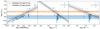 |
Fig. 6. Virial factor fσ derived from the DyBEL BLR fitting using σ-derived SMBH masses, as a function of the Hα line shape (left panel), the inclination angle in degrees (middle panel), and the opening angle in degrees (right panel). The average 1σ uncertainties are shown on the upper right of each panel. The orange dashed horizontal line and its 1σ range refer to f = 4.47, the virial factor in the scaling relations of Woo et al. (2015) from which we derived the SMBH masses to use as input to the fitting procedure. The blue dashed horizontal line and its 1σ range refer to the average Hα virial factor from our modelling: ⟨fσ, Hα⟩=1.44. For comparison, we plot the data points from Villafaña et al. (2023) together with a black solid line and a grey region denoting the best-fit relation and its intrinsic scatter. |
5.4. Targets fitted with the full model
Most of our targets (27/29) are well-fitted with the simpler, circular model, indicating that the data currently available – the line profiles, in particular, their peaks and wings – are fully consistent with a BLR dominated by Keplerian motion. This includes some sources with slightly asymmetric profiles, in particular where the wings are offset with respect to the core because the spectra have large enough flux uncertainties that the circular model is still a sufficiently good fit. However, the asymmetric shape of the line profiles for two of the targets cannot be fitted well with the circular model, partly due to the higher S/N in their spectra. Instead, for these targets, we use the more complex, full model, which allows anisotropic emission as well as radial motions. Fig. 7 shows the spectra and the fitted model profile for these two targets, ID#1 and ID#5 (SDSS J121843.39+153617.2 and Q 0226-1024 respectively). In the former case, we have removed the small bump that we concluded in Sect. 4.2 was likely due to [N II] λ6584. This still leaves a broad excess on the long wavelength side of the line profile. If we interpret the small bump as part of the Hα line, this only strengthens the results below because it increases the asymmetry. In ID#5, although the asymmetry is less obvious, the long wavelength wing is significantly stronger and more extended than the short wavelength wing.
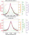 |
Fig. 7. Data (black points) and model (solid red line) Hα spectra derived from the best-fit BLR model of two SOFI z ∼ 2 targets fitted with the full model. The red-shaded regions show the 1σ error of the model spectra. The name of the target is shown on top of each panel. (a) Even after removing the bump on the right side of the Hα emission line, which we believe to be [N II] λ6584, SDSS J121843.39+153617.2 still shows an asymmetric Hα line profile which cannot be fitted with the circular model. (b) The Hα emission line of Q 0226–1024 shows an asymmetry in its wings which is better fitted with the full model. We also present the theoretical OH (sky) spectrum, the theoretical atmospheric profile, and the filter transmission profile of SOFI Ks band in orange, green, and purple lines, respectively. The sky and atmospheric profiles are normalised such that the maximum value is 1, and scaled by a factor of 2. We found that the observed asymmetries of both targets are within the high transmission regions of the SOFI Ks filter where no strong sky lines or atmospheric features are present. |
In order to assess whether there is a common cause underlying the asymmetric profiles in these objects, we compare their fitted parameters aided by the face-on and edge-on representations of their BLR models in Figs. 8 and 9. Of the asymmetry parameters, only the midplane transparency is similar for ID#1 and ID#5: ξ ∼ 0.5. This suggests that there is only moderate opacity in the midplane of both their BLRs. While there is little anisotropy in the emission for ID#5 (κ = −0.01), for ID#1 there is a preference for emission from the far side of the BLR (κ = −0.39). This overcomes the effect of the midplane opacity as can be seen in the edge-on projection of the BLR model in Fig. 8, where the size of the points, which represent clouds, indicates their relative observed flux: although there are slightly fewer points on the far side of the midplane due to its modest opacity, these blue-shifted points are larger than the red-shifted points, hence the former are brighter than the latter.
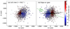 |
Fig. 8. The cloud distribution of the best-fit BLR model of ID#1 (SDSS J121843.39+153617.2) shown in two different views: (a) line-of-sight (LoS) or face-on view at the best-fit inclination angle i = 54.6° and (b) edge-on view. The PA of the BLR model to generate the cloud distribution is set so that the BLR is perpendicular to the UT4–UT1 baseline to achieve the maximum possible expected differential phase signal on the baseline. The BLR centre is positioned at the origin. The colour of each cloud refers to the LoS velocity, while the size of each cloud refers to the weight of each cloud on the total emission: the larger the size, the greater its contribution to the broad line emission. The green line on the edge-on view depicts the midplane of the BLR, while the black arrow depicts the LoS of the observer (i.e. the observer is on the +Δx direction). The LoS is tilted by i which is measured from the line perpendicular to the midplane. Since i > θ0, the observed flux spectrum is double-peaked. The number of clouds above and below the midplane are the same due to the small midplane opacity. However, the blueshifted clouds have a larger size than the redshifted clouds, indicating the preference of the BLR emission to originate from the far side of the BLR. This explains the relatively strong blueshifted peak of the flux spectrum compared to the redshifted bump. |
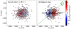 |
Fig. 9. Similar to Fig. 8 but for the cloud distribution of the best-fit BLR model of ID#5 (Q 0226–1024). The BLR clouds have almost equal sizes, pertaining to the lack of preference of the BLR emission to originate from either side. However, the moderate opacity on the midplane affects the blueshifted clouds more than the redshifted clouds, as indicated by the slightly lower number of blueshifted clouds compared to the redshifted clouds. This causes the redshifted wing of the Hα emission line to be slightly higher than the blueshifted wing. |
In terms of the geometry of the BLR, the angular distribution of the clouds for ID#1 is more concentrated towards the edges (γ = 3.9) than that of ID#5 (γ = 2.7). In addition, the model for ID#1 is dominated by radially moving clouds (fellip = 0.17) while that for ID#5 is more evenly shared between circular and elliptical/radial orbits (fellip = 0.41). Nevertheless, in both cases the radial motion is inwards (fflow < 0.5). Lastly, θe ∼ 20 and ∼36 for ID#1 and ID#5 respectively, suggesting that the elliptical orbits of the former are more elongated and so have higher radial velocities, but in neither case do these reach the maximum velocity allowed by the model.
In conclusion, for ID#1 we purport that the shape of the profile is due to a combination of projection effects resulting from i and θ0 combined with the effects induced by the asymmetry parameters. First, since i is greater than θ0 (54.6° versus 25.1°), the observed line profile is double-peaked due to the observed biconical structure of the BLR (Stock 2018). The inflowing motion means that clouds on the far side are blueshifted, which clouds on the near side are redshifted. In addition, since κ indicates a preference for the emission to originate from the far side of the BLR, the emission tracing the blueshifted part of the line profile is stronger than the redshifted side, leading to the two peaks having different strengths.
Compared to this, ID#5 exhibits less asymmetry in its Hα profile. The edge-on view of its BLR in Fig. 9 clearly shows that the blueshifted clouds are fewer in number than the redshifted clouds due to the moderate asymmetry affecting the former more than the latter. This results in an enhancement in the redshifted wing of the Hα emission line of ID#5.
6. Differential phase estimation
One of the main goals of this work is to estimate the strength of the differential phase signals of our z ∼ 2 AGNs to assess their observability with GRAVITY+. The differential phase is one of the most important observables in interferometric observations of AGNs (GRAVITY Collaboration 2018, 2020, 2024; GRAVITY+ Collaboration 2022). In our context, it is a spatially resolved kinematic signature; specifically, a measure of the astrometric shift of the photocentre of the BLR line emission with respect to that of the continuum as a function of wavelength. More details about the differential phase are presented in GRAVITY Collaboration (2020). A symmetric rotating BLR is expected to show an S-shape differential phase profile, which has been shown to be the case for several GRAVITY-observed AGNs (GRAVITY Collaboration 2018, 2020, 2023). However, some AGNs exhibit asymmetric differential phase profiles, which are explained in terms of asymmetry in the BLR, often combined with outflow motions in the BLR (GRAVITY Collaboration 2024).
We derive the expected differential phase of our targets for Hα since this is the only line observable in the K band (at z ∼ 2) where GRAVITY operates. We use the normalised line profile from the best-fit BLR model while adopting the same flux uncertainties as the data, and calculate the differential phase as a function of wavelength across the whole K band:
where Δϕλ is the differential phase measured in a wavelength channel λ, fλ is the normalised flux in that channel, u is the uv coordinate of the baseline, and xBLR,λ are the BLR photocentres. We calculate the 1σ uncertainty of the peak expected differential phase by randomly drawing values of relevant model parameters from the sampled posterior parameter space created during BLR model fitting. This is done 100 times to produce a distribution where the 16th, 50th, and 84th percentile of the peak expected differential phase is calculated.
The position angle PA (measured east of north) rotates the BLR within the sky plane and greatly influences the orientation of the differential phase signal. In order to make a comparative analysis between our targets, we are only interested in the highest possible peak differential phase for each. As such, we focus on the differential phase for the longest baseline, UT4–UT1, for which it is expected to be strongest. We therefore assume that the uv direction of the longest baseline of GRAVITY is parallel to the PA of the BLR model.
6.1. Expected differential phase signals and effect of fixed BH mass on the DyBEL BLR fitting
Estimating the expected differential phase as described above will provide important guidance in assigning priorities for observations with GRAVITY+, especially for a large sample of AGN. Here, we assessed the effectiveness of such a method for our z ∼ 2 targets, together with its caveats from the assumptions made during the BLR fitting.
Fig. 10 shows the Hα BLR size of our 29 targets as a function of the peak expected differential phase (ϕpeak) in logarithm. The peak expected differential phase values of all the targets and their 1σ errors are listed in Table B. The targets are divided into three categories: weak (ϕpeak< 1°), strong (1° < ϕpeak < 15°), and extreme (ϕpeak > 15°. The majority of the targets (23/29) have differential phase signals that go as high as > 1°. The strong targets (17/29), have signals with strengths between 1° − 15°, which is of comparable strength to the 1° for the z = 2.3 QSO observed with GRAVITY (Abuter et al. 2024). On the other hand, the weak targets (6/29) have signals that are comparable to those of the low redshift type 1 AGNs observed with GRAVITY (GRAVITY Collaboration 2018, 2020, 2021a). Most of the targets show a symmetric S-shape signal, as expected for a BLR with ordered rotation. This is a direct result of using the circular model for most sources. In contrast, for the two targets that were fitted with the full model, ID#1 and ID#5, we expect an asymmetric differential phase.
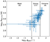 |
Fig. 10. Hα BLR size as a function of the peak expected differential phase in logarithm. The error bars correspond to their 1σ errors. The solid vertical lines pertain to the divisions categorising the targets into weak, strong, and extreme targets (see discussion in Sect. 6.1). The number of targets for each category is shown in parentheses. |
The expected differential phase is highly dependent on the assumed (fixed) SMBH mass when fitting the BLR model because the phase signal linearly scales with the BLR size, which is also related to the SMBH mass. However, we expect the SMBH mass not to affect the geometry and the virial factor. Some (6/29) of our targets have very strong differential phase signals (≥15°). We call these “extreme” targets because the SMBH masses derived from their dispersion σ are much larger than from their FWHM when using the equations from Woo et al. (2015). These targets have FWHM/σ < 1.25, indicating their line wings to be broad and prominent with respect to their narrow cores. Two of these “extreme” targets, ID#9 and ID#16 (HE 0320–1045 and 2QZ J031527.8-272645 respectively), show very strong narrow cores, with a narrow core to broad wing amplitude ratio > 10, while the other “extreme” targets have ratios in the range 0.1–7.0, similar to the non-extreme targets.
Indeed, Kollatschny & Zetzl (2011) argued that FWHM and σ are poor estimators of SMBH mass. They investigated this issue by looking at the turbulent and rotational velocities of several AGNs together with their line shape measurements. Their results suggest that the broadening of the line profiles is due to rotation, and the rotational velocity is a better estimator of SMBH mass than the line dispersion or FWHM. The reason is that AGNs with similar rotation velocities, for which the SMBH mases are the same, may show different values of FWHM/σ. In contrast, the SMBH masses calculated from their FWHM or σ may differ drastically. However, inferring the rotational velocity from the line profile in order to estimate the SMBH mass is outside the scope of this work. An independent and more accurate measurement of the SMBH masses for our targets is crucial to shed light on the size-luminosity relation and the efficacy of the rotation/turbulence interpretation versus the two-component BLR model, underlining the importance of the future GRAVITY+ observations of these targets.
7. Conclusions and future prospects
To prepare for the advent of GRAVITY+, we performed NTT/SOFI observations of type-1 AGN candidates in order to predict their expected differential phases and assess their priorities for GRAVITY+ observations. We focus on the 29 z ∼ 2 targets with prominent Hα emission lines. Among these are 17 for which we have also detected significant Hβ emission, and 2 with Hγ emission. We analyse the line profile shape (FWHM/σ) and fit BLR models using the DyBEL code. Our results yield the following conclusions:
-
Most of the Hα line profiles are highly non-Gaussian and so are fitted with two components: one for the narrow core, and another for the broad wings. This is reminiscent of the two-component BLR model, in which the wings represent an inner fast rotating BLR disc, and the lower velocity core represents an outer thicker part of the BLR. An alternative explanation is that the profile results from a convolution of rotation and turbulence, but in which the rotation is most easily seen via its impact in broadening the core of the profile.
-
The average σ-based Hα virial factor of our sample is fσ ∼ 1.44, which we attribute to the non-Gaussian shape of the emission lines. In contrast, we would expect to recover fσ = 4.47 (as used to derive the single-epoch SMBH masses) if our sample were to exhibit more Gaussian-like line profiles.
-
Our sample probes higher inclination i and higher disc thickness θ0 than those reported by Villafaña et al. (2023), and the values we found are consistent with anti-correlations between these parameters and the virial factor reported by those authors.
-
The line profiles of all except two of the targets, are well fitted with a circular simplification of the BLR model. The two targets that require the full model show asymmetry in their Hα line profiles, and our results suggest tentative evidence for radially dominated motions in these targets, with midplane obscuration and anisotropic emission contributing to the asymmetry in the observed line profiles.
-
The expected differential phase signal is an essential tool for assessing the future observing priorities of our targets with GRAVITY+. Among the 29 targets, 23 have strong signals, with six possessing expected differential phases > 15°. These “extreme” targets have very low FWHM/σ, highlighting concerns about applying scaling relations without accounting for differing line profiles because of the impact this has on the inferred SMBH mass. GRAVITY+ observations of these targets will provide an independent dynamical measurement of the SMBH in our targets and will not only further our understanding of varying BLR geometries at different epochs and luminosities but will provide a new baseline for future scaling relations.
Available from https://www.eso.org/sci/software/pipelines
Acknowledgments
J.S. acknowledges the National Science Foundation of China (12233001) and the National Key R&D Program of China (2022YFF0503401). This research has used the NASA/IPAC Extragalactic Database (NED), operated by the California Institute of Technology, under contract with the National Aeronautics and Space Administration. This research used the SIMBAD database operated at CDS, Strasbourg, France.
References
- Abuter, R., Allouche, F., Amorim, A., et al. 2024, Nature, 627, 281 [NASA ADS] [CrossRef] [Google Scholar]
- Acker, A., Köppen, J., Samland, M., & Stenholm, B. 1989, Messenger, 58, 44 [Google Scholar]
- Bentz, M. C., Denney, K. D., Grier, C. J., et al. 2013, ApJ, 767, 149 [Google Scholar]
- Bentz, M. C., Williams, P. R., Street, R., et al. 2021, ApJ, 920, 112 [NASA ADS] [CrossRef] [Google Scholar]
- Bischetti, M., Feruglio, C., Piconcelli, E., et al. 2021, A&A, 645, A33 [NASA ADS] [CrossRef] [EDP Sciences] [Google Scholar]
- Boizelle, B. D., Barth, A., Walsh, J. L., et al. 2019, ApJ, 881, 10 [NASA ADS] [Google Scholar]
- Boroson, T. 2005, ApJ, 130, 381 [CrossRef] [Google Scholar]
- Brotherton, M. S., Wills, B. J., Francis, P. J., & Steidel, C. 1994, ApJ, 430, 495 [NASA ADS] [Google Scholar]
- Burtscher, L., Davies, R. I., Graciá’-Carpio, J., et al. 2016, A&A, 586, A28 [NASA ADS] [CrossRef] [EDP Sciences] [Google Scholar]
- Canfield, R. C., & Puetter, R. 1981, ApJ, 390, 390 [Google Scholar]
- Carraro, R., Rodighiero, G., Cassata, P., et al. 2020, A&A, 642, A65 [EDP Sciences] [Google Scholar]
- Collin, S., Kawaguchi, T., Peterson, B. M., & Vestergaard, M. 2006, A&A, 456, 75 [NASA ADS] [CrossRef] [EDP Sciences] [Google Scholar]
- Crowther, P. A., & Bohannan, B. 1997, A&A, 317, 532 [NASA ADS] [Google Scholar]
- Dalla Bontá, E., Peterson, B. M., Bentz, M. C., et al. 2020, ApJ, 903, 112 [CrossRef] [Google Scholar]
- Di Matteo, T., Springel, V., & Hernquist, L. 2005, Nature, 433, 604 [NASA ADS] [CrossRef] [Google Scholar]
- Domínguez, A., Siana, B., Henry, A. L., et al. 2013, ApJ, 763, 145 [CrossRef] [Google Scholar]
- Dong, X., Wang, T., Wang, J., et al. 2008, MNRAS, 383, 581 [NASA ADS] [Google Scholar]
- Eisenhauer, F., Monnier, J. D., & Pfuhl, O. 2023, ARA&A, 61, 237 [NASA ADS] [CrossRef] [Google Scholar]
- Elitzur, M., Ho, L. C., & Trump, J. 2014, MNRAS, 438, 3340 [CrossRef] [Google Scholar]
- Ferrarese, L., & Ford, H. 2005, Space Sci. Rev., 116, 523 [Google Scholar]
- Ferrarese, L., & Merritt, D. 2000, ApJ, 539, L9 [Google Scholar]
- Fian, C., Jiménez-Vicente, J., Mediavilla, E., et al. 2024, ApJ, 972, L7 [NASA ADS] [CrossRef] [Google Scholar]
- Flesch, E. W. 2021, ArXiv e-prints [arXiv:2105.12985] [Google Scholar]
- Goodrich, R. 1990, ApJ, 355, 88 [NASA ADS] [CrossRef] [Google Scholar]
- GRAVITY Collaboration (Abuter, R., et al.) 2017, A&A, 602, A94 [NASA ADS] [CrossRef] [EDP Sciences] [Google Scholar]
- GRAVITY Collaboration (Sturm, E., et al.) 2018, Nature, 563, 657 [Google Scholar]
- GRAVITY Collaboration (Amorim, A., et al.) 2020, A&A, 643, A154 [NASA ADS] [CrossRef] [EDP Sciences] [Google Scholar]
- GRAVITY Collaboration (Amorim, A., et al.) 2021a, A&A, 648, A117 [NASA ADS] [CrossRef] [EDP Sciences] [Google Scholar]
- GRAVITY Collaboration (Amorim, A., et al.) 2021b, A&A, 654, A85 [NASA ADS] [CrossRef] [EDP Sciences] [Google Scholar]
- GRAVITY Collaboration (Amorim, A., et al.) 2023, A&A, 669, A14 [NASA ADS] [CrossRef] [EDP Sciences] [Google Scholar]
- GRAVITY Collaboration (Amorim, A., et al.) 2024, A&A, 684, A167 [NASA ADS] [CrossRef] [EDP Sciences] [Google Scholar]
- GRAVITY+ Collaboration (Abuter, R., et al.) 2022, Messenger, 189, 17 [NASA ADS] [Google Scholar]
- Greene, J. E., & Ho, L. C. 2004, ApJ, 610, 722 [NASA ADS] [CrossRef] [Google Scholar]
- Greene, J. E., Peng, C. Y., Kim, M., et al. 2010, ApJ, 721, 26 [NASA ADS] [CrossRef] [Google Scholar]
- Grier, C. J., Peterson, B. M., Horne, K., et al. 2013, ApJ, 764, 47 [NASA ADS] [CrossRef] [Google Scholar]
- Gültekin, K., Richstone, D. O., Gebhardt, K., et al. 2009, ApJ, 698, 198 [Google Scholar]
- Harrison, C. M. 2017, Nat. Astron., 1, 65 [Google Scholar]
- Heckman, T., & Best, P. 2014, ARA&A, 52, 589 [Google Scholar]
- Horne, K. 1986, PASP, 98, 609 [Google Scholar]
- Kaspi, S., Brandt, W. N., Maoz, D., et al. 2021, ApJ, 915, 129 [NASA ADS] [CrossRef] [Google Scholar]
- Kollatschny, W., & Zetzl, M. 2011, Nature, 470, 366 [NASA ADS] [CrossRef] [Google Scholar]
- Kollatschny, W., & Zetzl, M. 2013, A&A, 549, A100 [NASA ADS] [CrossRef] [EDP Sciences] [Google Scholar]
- Kormendy, J., & Ho, L. C. 2013, ARA&A, 51, 511 [Google Scholar]
- Krawczyk, C. M., Richards, G. T., Mehta, S. S., et al. 2013, ApJS, 206, 4 [Google Scholar]
- Kuhn, L., Shangguan, J., Davies, R., et al. 2024, A&A, 684, A52 [NASA ADS] [CrossRef] [EDP Sciences] [Google Scholar]
- Kuo, C. Y., Braatz, J. A., Impellizzeri, C. M. V., et al. 2020, MNRAS, 498, 1609 [NASA ADS] [CrossRef] [Google Scholar]
- Kwan, J., & Krolik, J. 1981, ApJ, 250, 478 [NASA ADS] [CrossRef] [Google Scholar]
- La Mura, G., Popović, L. Č., Ciroi, S., Rafanelli, P., & Ilić, D. 2007, ApJ, 671, 104 [NASA ADS] [CrossRef] [Google Scholar]
- Lapi, A., Raimundo, S., Aversa, R., et al. 2014, ApJ, 782, 69 [NASA ADS] [CrossRef] [Google Scholar]
- Li, J. I. H., Li, H., Shen, Y., et al. 2023, ApJ, 954, 173 [NASA ADS] [CrossRef] [Google Scholar]
- Ludwig, R. R., Greene, J. E., Barth, A. J., & Ho, L. 2012, ApJ, 756, 51 [NASA ADS] [CrossRef] [Google Scholar]
- Lyke, B. W., Higley, A. N., McLane, J. N., et al. 2020, ApJS, 250, 8 [NASA ADS] [CrossRef] [Google Scholar]
- Madau, P., & Dickinson, M. 2014, ARA&A, 52, 415 [Google Scholar]
- Maheson, G., Maiolino, R., Curti, M., et al. 2024, MNRAS, 527, 8213 [Google Scholar]
- Marsden, C., Shankar, F., Ginolfi, M., & Zubovas, K. 2020, Front. Phys., 8, 61 [NASA ADS] [CrossRef] [Google Scholar]
- Martín-Navarro, I., Burchett, J. N., & Mezcua, M. 2020, MNRAS, 491, 1311 [Google Scholar]
- Marziani, P., Negrete, C. A., Dultzin, D., et al. 2017, Front. Astron. Space Sci., 4, 16 [NASA ADS] [CrossRef] [Google Scholar]
- Monroe, T. R., Prochaska, J. X., Tejos, N., et al. 2016, Front. Astron. Space Sci., 152, 25 [Google Scholar]
- Nagoshi, S., Iwamuro, F., Yamada, S., et al. 2024, MNRAS, 529, 393 [NASA ADS] [CrossRef] [Google Scholar]
- Oh, S., Colless, M., Barsanti, S., et al. 2024, MNRAS, 531, 4017 [NASA ADS] [CrossRef] [Google Scholar]
- Onken, C. A., Wolf, C., Hon, W. J., et al. 2023, PASA, 40, e010 [NASA ADS] [CrossRef] [Google Scholar]
- Osorno, J., Nagar, N., Richtler, T., et al. 2023, A&A, 679, A37 [NASA ADS] [CrossRef] [EDP Sciences] [Google Scholar]
- Pancoast, A., Brewer, B. J., & Treu, T. 2014, MNRAS, 445, 3055 [Google Scholar]
- Park, D., Barth, A. J., Ho, L. C., & Laor, A. 2022, ApJS, 258, 38 [NASA ADS] [CrossRef] [Google Scholar]
- Peterson, B. M. 1993, PASP, 105, 247 [NASA ADS] [CrossRef] [Google Scholar]
- Peterson, B. M. 2008, ApJ, 52, 240 [Google Scholar]
- Peterson, B. M., Ferrarese, L., Gilbert, K. M., et al. 2004, ApJ, 613, 682 [Google Scholar]
- Planck Collaboration XIII. 2016, A&A, 594, A13 [NASA ADS] [CrossRef] [EDP Sciences] [Google Scholar]
- Popović, L. Č., Mediavilla, E., Bon, E., & Ilić, D. 2004, A&A, 423, 909 [NASA ADS] [CrossRef] [EDP Sciences] [Google Scholar]
- Prieto, A., Rodríguez-Ardila, A., Panda, S., & Marinello, M. 2022, MNRAS, 510, 1010 [Google Scholar]
- Raimundo, S. I., Pancoast, A., Vestergaard, M., Goad, M. R., & Barth, A. J. 2019, MNRAS, 489, 1899 [Google Scholar]
- Reddy, N. A., Kriek, M., Shapley, A. E., et al. 2015, ApJ, 806, 256 [NASA ADS] [Google Scholar]
- Saglia, R. P., Opitsch, M., Erwin, P., et al. 2016, ApJ, 818, 47 [Google Scholar]
- Shapley, A. E., Sanders, R. L., Salim, S., et al. 2022, ApJ, 926, 145 [NASA ADS] [CrossRef] [Google Scholar]
- Shen, Y., & Liu, X. 2012, ApJ, 753, 125 [NASA ADS] [CrossRef] [Google Scholar]
- Silk, J. 2013, ApJ, 772, 112 [Google Scholar]
- Skilling, J. 2004, in Bayesian Inference and Maximum Entropy Methods in Science and Engineering: 24th International Workshop on Bayesian Inference and Maximum Entropy Methods in Science and Engineering, eds. R. Fischer, R. Preuss, & U. V. Toussaint, AIP Conf. Ser., 735, 395 [NASA ADS] [CrossRef] [Google Scholar]
- Speagle, J. S. 2020, MNRAS, 493, 3132 [Google Scholar]
- Stock, M. R. 2018, Master’s Thesis, Technische Universität München [Google Scholar]
- Storchi-Bergmann, T., Schimoia, J. D. S., Peterson, B. M., et al. 2017, ApJ, 835, 236 [NASA ADS] [Google Scholar]
- Storey-Fisher, K., Hogg, D. W., Rix, H.-W., et al. 2024, ApJ, 964, 69 [NASA ADS] [CrossRef] [Google Scholar]
- Suh, H., Civano, F., Trakhtenbrot, B., et al. 2020, ApJ, 889, 32 [NASA ADS] [CrossRef] [Google Scholar]
- Tacconi, L. J., Genzel, R., & Sternberg, A. 2020, ARA&A, 58, 157 [NASA ADS] [CrossRef] [Google Scholar]
- Terrazas, B. A., Bell, E. F., Woo, J., & Henriques, B. 2017, ApJ, 844, 170 [NASA ADS] [CrossRef] [Google Scholar]
- Trakhtenbrot, B., Ricci, C., Koss, M. J., et al. 2017, MNRAS, 470, 800 [NASA ADS] [CrossRef] [Google Scholar]
- Vestergaard, M., & Peterson, B. 2006, ApJ, 641, 689 [NASA ADS] [Google Scholar]
- Villafaña, L., Williams, P. R., Treu, T., et al. 2023, ApJ, 948, 95 [CrossRef] [Google Scholar]
- Wang, S., Shen, Y., Jiang, L., et al. 2019, ApJ, 882, 4 [CrossRef] [Google Scholar]
- Wang, S., Shen, Y., Jiang, L., et al. 2020, ApJ, 903, 51 [NASA ADS] [CrossRef] [Google Scholar]
- Whittle, M. 1985, ApJ, 213, 1 [Google Scholar]
- Woo, J. H., Yoon, Y., Park, S., Park, D., & Kim, S. C. 2015, ApJ, 801, 38 [NASA ADS] [CrossRef] [Google Scholar]
- Wu, J., Wu, Q., Xue, H., Lei, W., & Lyu, B. 2023, ApJ, 950, 106 [NASA ADS] [CrossRef] [Google Scholar]
- Yesuf, H. M., & Ho, L. C. 2020, ApJ, 901, 42 [NASA ADS] [CrossRef] [Google Scholar]
- Zhang, X.-G. 2011, ApJ, 741, 104 [NASA ADS] [Google Scholar]
- Zhu, L., Zhang, S. N., & Tang, S. 2009, ApJ, 700, 1173 [NASA ADS] [Google Scholar]
Appendix A: Target list and emission line properties
All high-redshift targets with clear Hα detection from their SOFI spectra.
Emission line measurements of our high-redshift SOFI targets in the Hα spectral region.
Emission line measurements of our high-redshift SOFI targets for Hβ, [OIII] doublet, and Hγ emission lines.
Emission line measurements of three high-redshift SOFI targets in the Hβ region where the Hα and Hβ line shapes are not fixed to be similar as discussed in Sec. 4.1.
Appendix B: Summary of DyBEL BLR fitting results
Results of fitting the BLR model to the line profiles.
All Tables
Emission line measurements of our high-redshift SOFI targets in the Hα spectral region.
Emission line measurements of our high-redshift SOFI targets for Hβ, [OIII] doublet, and Hγ emission lines.
Emission line measurements of three high-redshift SOFI targets in the Hβ region where the Hα and Hβ line shapes are not fixed to be similar as discussed in Sec. 4.1.
All Figures
|
Fig. 1. Representative line decomposition results for three of our SOFI z ∼ 2 targets. Each row refers to a different target (QBQS J051411.75-190139.4, SDSS J220245.60-024407.1, and SDSS J121843.39+153617.2), while each column refers to a different spectral region (Hβ and Hα). The observed data are shown in blue, while the cumulative best-fit spectrum is shown as an orange solid line. The different coloured lines pertain to different components in the line decomposition, as shown in the legend. Some of our targets have strong Fe II and even clear Hγ emission, as shown in the Hβ region of QBQS J051411.75-190139.4 (panel a). On the other hand, a few targets have prominent (S/N > 3) [O III] features similar to SDSS J220245.60-024407.1 (panel c). Both of these objects were observed with the GRF filter, hence other Balmer lines aside from Hα are detected. On the other hand, SDSS J121843.39+153617.2 was observed with the Ks filter (panel e). Its Hα spectrum shows a weak [N II] λ6584 feature (see Sect. 4.2). |
| In the text | |
|
Fig. 2. Ratio of FWHM to σ (line shape) of Hα lines fitted with the double-Gaussian model as a function of FWHM. The Gaussian limit (FWHM ∼ 2.35σ) is shown as a horizontal grey solid line. The error bars denote 1σ uncertainties. For comparison, we plot the theoretical line width ratios of rotational line broadened Lorentzian profiles for Hα (black dashed lines and markers) and Hβ (grey dashed lines and markers) which were taken from Kollatschny & Zetzl (2011) and Kollatschny & Zetzl (2013). Different markers pertain to different FWHMs of the Lorentzian profiles. |
| In the text | |
|
Fig. 3. Ratio between Hα and Hβ luminosity as a function of Hα luminosity. The blue (orange) points show the targets that are fitted with a double (single) Gaussian model. We remove two targets (from the three exceptions in Table A.4) whose Hβ lines cannot be fitted with the same number of Gaussian components and line shape as that of Hα. The error bars are 1σ uncertainties. |
| In the text | |
|
Fig. 4. Logarithm of bolometric luminosity as a function of the logarithm of BH mass. For the SOFI z ∼ 2 targets (This work, blue data points), the Lbol are estimated from Hα, while the MBH are estimated using Eq. (6) of Woo et al. (2015) which uses the dispersion (σ) and Hα luminosity as inputs. The typical error of log Lbol is shown as the blue vertical error bar on the lower right of the panel. For comparison, we show the sample of z = 1.5–2.5 with Lbol < 47 as orange points (Suh et al. 2020) and high-luminosity quasars from the WISSH survey as green points (Bischetti et al. 2021). The grey dashed lines pertain to the loci of the same Eddington ratio: λEdd = 0.01, 0.1, 1, and 10. For the WISSH quasars, we assume a BH mass uncertainty of ∼0.47 dex following the prescription for the 1σ relative uncertainty of single-epoch BH mass estimates from Vestergaard & Peterson (2006). However, we do not include the systematic uncertainties for the absolute calibration of RM masses. |
| In the text | |
|
Fig. 5. Normalised (i.e. independently for each histogram such that the area under the histogram is 1) histograms showing in blue the summed posterior distributions of the BLR parameters from the best fits to all the z ∼ 2 targets. The panels correspond to (a) the radial distribution of BLR clouds, (b) the inclination angle, (c) the opening angle, with the minimum and maximum values defining the thin disc and spherical shape, respectively, (d) the ratio between the minimum and mean Hα BLR radius, and (e) the mean (emissivity) Hα BLR radius. |
| In the text | |
|
Fig. 6. Virial factor fσ derived from the DyBEL BLR fitting using σ-derived SMBH masses, as a function of the Hα line shape (left panel), the inclination angle in degrees (middle panel), and the opening angle in degrees (right panel). The average 1σ uncertainties are shown on the upper right of each panel. The orange dashed horizontal line and its 1σ range refer to f = 4.47, the virial factor in the scaling relations of Woo et al. (2015) from which we derived the SMBH masses to use as input to the fitting procedure. The blue dashed horizontal line and its 1σ range refer to the average Hα virial factor from our modelling: ⟨fσ, Hα⟩=1.44. For comparison, we plot the data points from Villafaña et al. (2023) together with a black solid line and a grey region denoting the best-fit relation and its intrinsic scatter. |
| In the text | |
|
Fig. 7. Data (black points) and model (solid red line) Hα spectra derived from the best-fit BLR model of two SOFI z ∼ 2 targets fitted with the full model. The red-shaded regions show the 1σ error of the model spectra. The name of the target is shown on top of each panel. (a) Even after removing the bump on the right side of the Hα emission line, which we believe to be [N II] λ6584, SDSS J121843.39+153617.2 still shows an asymmetric Hα line profile which cannot be fitted with the circular model. (b) The Hα emission line of Q 0226–1024 shows an asymmetry in its wings which is better fitted with the full model. We also present the theoretical OH (sky) spectrum, the theoretical atmospheric profile, and the filter transmission profile of SOFI Ks band in orange, green, and purple lines, respectively. The sky and atmospheric profiles are normalised such that the maximum value is 1, and scaled by a factor of 2. We found that the observed asymmetries of both targets are within the high transmission regions of the SOFI Ks filter where no strong sky lines or atmospheric features are present. |
| In the text | |
|
Fig. 8. The cloud distribution of the best-fit BLR model of ID#1 (SDSS J121843.39+153617.2) shown in two different views: (a) line-of-sight (LoS) or face-on view at the best-fit inclination angle i = 54.6° and (b) edge-on view. The PA of the BLR model to generate the cloud distribution is set so that the BLR is perpendicular to the UT4–UT1 baseline to achieve the maximum possible expected differential phase signal on the baseline. The BLR centre is positioned at the origin. The colour of each cloud refers to the LoS velocity, while the size of each cloud refers to the weight of each cloud on the total emission: the larger the size, the greater its contribution to the broad line emission. The green line on the edge-on view depicts the midplane of the BLR, while the black arrow depicts the LoS of the observer (i.e. the observer is on the +Δx direction). The LoS is tilted by i which is measured from the line perpendicular to the midplane. Since i > θ0, the observed flux spectrum is double-peaked. The number of clouds above and below the midplane are the same due to the small midplane opacity. However, the blueshifted clouds have a larger size than the redshifted clouds, indicating the preference of the BLR emission to originate from the far side of the BLR. This explains the relatively strong blueshifted peak of the flux spectrum compared to the redshifted bump. |
| In the text | |
|
Fig. 9. Similar to Fig. 8 but for the cloud distribution of the best-fit BLR model of ID#5 (Q 0226–1024). The BLR clouds have almost equal sizes, pertaining to the lack of preference of the BLR emission to originate from either side. However, the moderate opacity on the midplane affects the blueshifted clouds more than the redshifted clouds, as indicated by the slightly lower number of blueshifted clouds compared to the redshifted clouds. This causes the redshifted wing of the Hα emission line to be slightly higher than the blueshifted wing. |
| In the text | |
|
Fig. 10. Hα BLR size as a function of the peak expected differential phase in logarithm. The error bars correspond to their 1σ errors. The solid vertical lines pertain to the divisions categorising the targets into weak, strong, and extreme targets (see discussion in Sect. 6.1). The number of targets for each category is shown in parentheses. |
| In the text | |
Current usage metrics show cumulative count of Article Views (full-text article views including HTML views, PDF and ePub downloads, according to the available data) and Abstracts Views on Vision4Press platform.
Data correspond to usage on the plateform after 2015. The current usage metrics is available 48-96 hours after online publication and is updated daily on week days.
Initial download of the metrics may take a while.