| Issue |
A&A
Volume 693, January 2025
|
|
|---|---|---|
| Article Number | A176 | |
| Number of page(s) | 15 | |
| Section | Extragalactic astronomy | |
| DOI | https://doi.org/10.1051/0004-6361/202450451 | |
| Published online | 15 January 2025 | |
JWST ERS Program Q3D: The pitfalls of virial black hole mass constraints shown for a z ∼ 3 quasar with an ultramassive host
1
Zentrum für Astronomie der Universität Heidelberg, Astronomisches Rechen-Institut Mönchhofstr, 12-14 69120 Heidelberg, Germany
2
Department of Physics, Rhodes College, Memphis, TN 38112, USA
3
Department of Physics and Astronomy, Bloomberg Center, Johns Hopkins University, Baltimore, MD 21218, USA
4
Institute for Advanced Study, Princeton, NJ 08540, USA
5
Department of Astronomy and Joint Space-Science Institute, University of Maryland, College Park, MD 20742, USA
6
Caltech/IPAC, 1200 E. California Blvd, Pasadena, CA 91125, USA
7
Max-Planck-Institut für Extraterrestrische Physik, Giessenbachstrasse 1, D-85748 Garching, Germany
8
CAS Key Laboratory for Research in Galaxies and Cosmology, Department of Astronomy, University of Science and Technology of China, Hefei, Anhui 230026, China
9
School of Astronomy and Space Sciences, University of Science and Technology of China, Hefei 230026, China
10
MIT Kavli Institute for Astrophysics and Space Research, Massachusetts Institute of Technology, Cambridge, MA 02139, USA
11
Steward Observatory, University of Arizona, 933 N. Cherry Ave., Tucson, AZ 85721, USA
⋆ Corresponding author; c.bertemes@uni-heidelberg.de
Received:
19
April
2024
Accepted:
13
November
2024
We present observations with the Mid-InfraRed Instrument (MIRI) and Near-InfraRed Spectrograph (NIRSpec) on board the James Webb Space Telescope (JWST), targeting the extremely red quasar J165202.64+172852.3 at z = 2.948 (dubbed J1652). As one of the most luminous quasars known to date, it drives powerful outflows and hosts a clumpy starburst, in the midst of several interacting companions. We estimated the black hole (BH) mass of the system based on the broad Hα and Hβ lines, as well as the broad Paβ emission in the infrared and Mg II in the ultraviolet. We recovered a very broad range of mass estimates, with individual constraints ranging between log MBH ∼ 9 and 10.2, which is extended further if we impose a uniform broad line region geometry at all wavelengths. The large spread may be caused by several factors: uncertainties on measurements (insufficient sensitivity to detect the broadest component of the faint Paschen β line, spectral blending, ambiguities in the broad or narrow component distinction, etc.), lack of virial equilibrium, and uncertainties on the luminosity-inferred size of the broad line region (BLR). The exotic nature of our target (luminous, starburst, powerful outflows, high accretion rate, and dusty centre) is another likely contribution to the large uncertainties. We broadly constrained the stellar mass of J1652 by fitting the spectral energy distribution, which suggests that the host is extremely massive, at ∼1012.1 M⊙, with a 1.1 dex uncertainty at > 1 dex above the characteristic mass of the Schechter fit to the z = 3 stellar mass function. Notably, J1652’s central BH might be interpreted as being either over-massive or in line with the BH mass–stellar mass relation, depending on the choice of assumptions. The recovered Eddington ratio varies accordingly, but it exceeds 10% in any case. We set our results into context by providing an extensive overview and discussion of recent literature results and their associated assumptions. Our findings provide an important demonstration of the uncertainties inherent in the virial BH mass estimates of individual objects, which are of particular relevance in the JWST era, given the increasing number of studies on rapidly accreting quasars at high redshift.
Key words: methods: observational / galaxies: evolution / galaxies: high-redshift / quasars: general / quasars: supermassive black holes
© The Authors 2025
 Open Access article, published by EDP Sciences, under the terms of the Creative Commons Attribution License (https://creativecommons.org/licenses/by/4.0), which permits unrestricted use, distribution, and reproduction in any medium, provided the original work is properly cited.
This article is published in open access under the Subscribe to Open model. Subscribe to A&A to support open access publication.
1. Introduction
Measuring the masses of supermassive black holes (SMBHs) is a necessary ingredient for understanding their growth, which is thought to be connected to galaxy evolution. In the Local Universe, the existence of tight correlations between central black hole (BH) masses MBH and host galaxy properties, such as stellar or bulge mass (M⋆/Mbulge) and stellar velocity dispersion (σ⋆) has been known for over two decades (Gebhardt et al. 2000; Ferrarese & Merritt 2000; see also Kormendy & Ho 2013, for a review), with the scatter being smallest for the MBH–σ⋆ relation (∼0.4 dex; see Woo et al. 2013). Studying the redshift evolution of these scaling relations offers insights into the co-evolution between galaxies and their SMBHs throughout cosmic time. While the correlation between BH masses and stellar masses is less tight than those with bulge properties or σ⋆, it offers the advantage that the total stellar mass is more directly measurable, especially at high redshift. However, an open question remains as to if and how the relation evolves with redshift, and whether different populations of active galactic nuclei (AGNs) harbour SMBHs that are systematically over- or under-massive with respect to their host galaxy (e.g. depending on the AGN selection method applied or the large-scale environment).
At cosmic noon (z ∼ 1 − 3), some studies have found BH masses exceeding those predicted by the local MBH–σ⋆ relation by a factor of 1.5 − 7 (Peng et al. 2006; Decarli et al. 2010; Merloni et al. 2010). Others have suggested the local relation was already in place (Schindler et al. 2016; Suh et al. 2020; Li et al. 2021, 2023) or reported mixed results or strictly a mild evolution scenario (Poitevineau et al. 2023; Tanaka et al. 2024). With the advent of the James Webb Space Telescope (JWST), there have been a number of recent claims that the earliest galaxies harbour over-massive BHs, with respect to the local relation between BH mass and stellar mass (Farina et al. 2022; Goulding et al. 2023; Harikane et al. 2023; Maiolino et al. 2024; Pacucci et al. 2023; Stone et al. 2024; Übler et al. 2024; Yue et al. 2024a); however, there are other studies that support more moderate BH masses in lower-luminosity AGNs (Izumi et al. 2018, 2019, 2021; Ding et al. 2023). These observations are of particular interest for the study of SMBH growth, potentially offering an opportunity to discriminate between different theoretical BH formation channels (see e.g. Bogdán et al. 2024; Goulding et al. 2023; Natarajan et al. 2024, and the review by Inayoshi et al. 2020). With a large number of ‘little red dots’, which are newly identified AGN candidates in JWST fields (Matthee et al. 2024; Juodžbalis et al. 2023; Labbe et al. 2023; Langeroodi & Hjorth 2023; Greene et al. 2024; Yang et al. 2023; Barro et al. 2024), the field is rapidly evolving as follow-up campaigns are conducted and datasets expanded.
However, such analyses are complicated by selection biases, measurement uncertainties, and the necessity of relying on assumptions motivated by low-redshift studies (e.g. Lauer et al. 2007; Volonteri et al. 2023; Zhang et al. 2023; Li et al. 2024). At the highest redshifts, neither direct dynamical measurements nor reverberation mapping (RM) measurements are available. As a result, the masses of BHs are typically inferred via the MBH–σ⋆ relation (Kormendy & Ho 2013) or via the kinematics of the orbiting gas in the broad line region (BLR), based on the virial theorem (e.g. Kaspi et al. 2000). Both methods come with their respective challenges. The BH masses based on the MBH–σ⋆ relation established for elliptical AGNs with suppressed star formation are found to be over-predicted with respect to direct dynamical measurements for the general population of X-ray AGNs (Gliozzi et al. 2024); moreover, they cannot (by definition) be used to determine whether a given BH is over- or under-massive for its host. There are several caveats associated with the virial method as well: in addition to measurement uncertainties, the unknown structure of the BLR introduces a scaling factor that is poorly constrained (e.g. Onken et al. 2004), the size of the BLR needs to be estimated via scaling relations in the absence of reverberation mapping observations, and the condition of virial equilibrium may not be satisfied in systems with inflowing or outflowing gas (Richards et al. 2011; Coatman et al. 2017; Fries et al. 2024). Additionally, calibrations have been made mostly based on observations of low-redshift AGNs, which may not directly be applicable to high-z quasars. For instance, Abuter et al. (2024) recently succeeded in dynamically measuring the BH mass of a z = 2.3 quasar with the GRAVITY+ instrument; they found their corresponding virial BH mass measurement needed a correction to the BLR size to agree with the dynamical constraint.
In this work, we test the self-consistency of single-epoch virial BH mass constraints in the extreme case of a rapidly accreting quasar near cosmic noon (z ∼ 3) with vigorous outflows, by using four different broad lines as a tracer: Mg II from the archival Sloan Digital Sky Survey (SDSS) spectrum, Hα, Hβ, and Paschen β (Paβ) from JWST observations in the near- and mid-infrared (NIR-MIR). Our target is taken from the JWST Early Release Science program Q3D (Wylezalek et al. 2022), which targeted three red quasars at 0.4 < z < 3 to study their spatially resolved physical properties and investigate their impact on their hosts, using the integral field unit (IFU) modes of the Near-InfraRed Spectrograph (NIRSpec; Jakobsen et al. 2022) and the Mid-InfraRed Instrument (MIRI; Rieke et al. 2015). The highest redshift target in the sample, SDSS J165202.64+172852.3 at z ∼ 3, is classified as an extremely red quasar. Extremely red quasars (ERQs; Hamann et al. 2017) are a fascinating population of unusually luminous AGNs identified at high redshift via their ultraviolet (UV) to NIR colours that resemble dust-obscured galaxies (Dey et al. 2008). They are found in massive host galaxies (Zakamska et al. 2019) and drive extreme ionised outflows with speeds up to ∼6000 km/s (Zakamska et al. 2016; Perrotta et al. 2019). In the picture of the AGN life cycle, they are thought to constitute an early and short-lived ‘blow-out’ phase of AGN activity, in the process of clearing out central dust that was funnelled to the inner regions, along with a gas inflow triggering the AGN.
The object of this work, J1652, is a particularly spectacular example of an ERQ. At a bolometric luminosity of 5 × 1047 erg/s (Perrotta et al. 2019), it is one of the brightest sources at its redshift z = 2.94 – and thus in the entire Universe, given that it resides in the epoch of peak quasar activity at 2 < z < 3 (Richards et al. 2006). It hosts both powerful galaxy-wide ionised outflows reaching ∼3000 km/s (Alexandroff et al. 2018; Vayner et al. 2021) and clumpy starbursting regions (Vayner et al. 2023). Furthermore, it is flanked by three spectroscopically confirmed interacting companion galaxies within projected distances of ≤15 kpc. It also resides within (potentially) one of the densest regions at its redshift (Wylezalek et al. 2022). The stellar mass of J1652 can be roughly estimated via its k-corrected B-Band luminosity and assuming a mass-to-light ratio of 0.4 − 1.4 at z = 3 (Maraston 2005), suggesting the system to be highly massive with a stellar mass of 1011.4 − 12.4 M⊙ (Zakamska et al. 2019). This may, however, be over-predicted given the strong quasar contribution. In this work, we leverage the JWST observations of the rest-frame optical and NIR emission of J1652 to infer further constraints on the stellar mass via SED fitting and we derive the BH mass via the broad Balmer lines as well as the Paβ line in the NIR with a comparison to UV-based constraints via Mg II.
The NIR Paschen lines are a valuable alternative kinematic tracer to the Balmer lines for deriving BH masses (see e.g. Lamperti et al. 2017; Mejía-Restrepo et al. 2022). Due to their lower sensitivity to dust extinction, the Paschen lines have been found to reveal a ‘hidden’ BLR missed by optical lines in some AGNs (Veilleux et al. 1997a,b, 1999; Lamperti et al. 2017). Further, hydrogen line ratios involving the Paschen lines can be used as a tracer for dust attenuation (Kim & Im 2018; Reddy et al. 2023), analogously to the Balmer decrement. In local star-forming galaxies, the combination of the Paβ and Hα line can trace larger optical depths, with inferred AV values exceeding those recovered by the optical Balmer decrement Hα / Hβ by as much as > 1 mag (Liu et al. 2013; Giménez-Arteaga et al. 2022) for a fixed attenuation law. However, the Paβ emission is intrinsically substantially fainter than Hα, rendering its measurements more challenging.
Our target, J1652, benefits from an existing SDSS spectrum (on this basis, it was classed as an extremely red quasar), which we can use to include a UV-based BH mass constraint based on Mg II in our comparison of different broad line tracers. Given their accessibility at high redshift, UV emission lines have frequently been used for studying virial BH masses at early cosmic times (McLure & Dunlop 2004; Vestergaard & Osmer 2009; Pensabene et al. 2020; Farina et al. 2022), although they are more sensitive to dust than optical/IR lines. The Mg II line is considered one of the most reliable tracers in the UV, while the C IV line profile is frequently dominated by non-gravitational effects (Baskin & Laor 2005; Mejía-Restrepo et al. 2016; Abuter et al. 2024; Coatman et al. 2016). In a recent JWST study of a merging quasar at z = 6, Loiacono et al. (2024) found a good agreement between the BH mass estimates based on the Balmer lines and inferred from Mg II at the level of < 0.15 dex. Similarly, Bosman et al. (2024) found a consistency between BH masses derived via Hα, Mg II, and the Paschen lines in a z = 7 quasar, accreting at 40% of the Eddington ratio. In this paper, we conduct a similar comparison in the case of a rapidly growing, potentially merging quasar with powerful outflows, and we conclude with a discussion summarising differences in methodology between different high-z studies of BH masses.
The paper is organised as follows. Section 2 describes the observations, data reduction and methods (fitting the spectral energy distribution and lines, virial BH mass measurements). Section 3 is dedicated to the presentation of our results on the inferred masses of J1652’s host galaxy and SMBH. In Section 4, we put our results into context by providing an overview and discussion of different high-redshift studies. Finally, we summarise our findings and conclusions in Section 5. Throughout this work, we use a ΛCDM cosmology defined by ΩΛ = 0.7, Ωm = 0.3, and H0 = 70 km s−1 Mpc−1.
2. Observations and Methods
2.1. JWST observations and data reduction
On 12 March 2023, JWST/MIRI observations of J1652 were taken using the Medium Resolution Spectrograph (MRS; Wells et al. 2015; Argyriou et al. 2023) and the SHORT grating configuration, with a wavelength coverage of 4.9 − 5.7 μm, 4.9 − 5.8 μm, 11.6 − 13.5 μm and 17.7 − 20.9 μm in Channels 1 through to 4. We used a four-point dither pattern for the science exposures. Dedicated background exposures were also obtained, using a single dither. The total on-source exposure time was 11084.9 s, and the background exposure time was 2771.2 s. This paper focuses on the channel 1 observations containing the Paβ line, for which the aperture spans 17 × 20 pixels of 1.69 ⋅ 10−2 arcsec2.
We reduced the MIRI MRS data with version 1.15.2 of the JWST pipeline1 and version 11.18.1 and context 1274 of the Calibration Reference Data System (CRDS). Here, we briefly summarise the modifications applied to the default pipeline. In stage 1 of the data reduction pipeline, we used the following jump settings (of which some are motivated by the procedure in Spilker et al. 2023): rejection_threshold is lowered to 3.5σ and min_jump_to_flag_neighbors to 8σ. We also turned on expand_large_events and use_ellipses, but switch off sat_required_snowball. The min_jump_area was set to 12 continuous pixels and we used values of 10, 20, 1000 and 3000 for the keywords after_jump_flag_dn1, after_jump_flag_time1, after_jump_flag_dn2, and after_jump_flag_time2, which relate to the duration for which a jump keeps being flagged in subsequent integrations after being identified. In stage 2 of the pipeline, we switched on the pixel replacement step, where pixels flagged as ‘bad’ were replaced via an interpolation using the values of neighbouring good pixels. For building the cubes, we use the ‘emsm’ algorithm, which improved spectral oscillations compared to the default ‘drizzle’ routine, whilst spatially smoothing the data and thus leading to a slightly larger point spread function (PSF). We used the master_background subtraction in stage 3, meaning that a ‘master’ spectrum is subtracted (as opposed to an image-by-image subtraction in stage 2). We also used the outlier detection in step 3 and flag neighbouring spaxels with the outlier_detection.grow option set to 3.
In this work, we also used our complementary NIRSpec observations of J1652 to compare its central Hα emission to that from Paβ present in the MIRI data. The NIRSpec data, along with the adopted data reduction procedure, are presented in Vayner et al. (2023, 2024). The data were obtained with the G235H/F170LP grating/filter combination. The total exposure time spent on-source was 16412.5 s and a nine-point cyclic dithering pattern was used. The spectral resolution was R ∼ 2700 over the observed wavelength range of 1.66–3.05 μm.
2.2. Ancillary data
J1652 has been observed with the Gemini Near-Infrared Spectrograph (GNIRS) mounted at Gemini-North (PI: Alexandroff; Alexandroff et al. 2018; Perrotta et al. 2019), whose coverage includes the Mg II line in the restframe UV. We used the latter to complement the virial BH mass estimates derived from our JWST observations covering rest-frame optical/NIR lines (Hα, Hβ and Paβ). The GNIRS data were obtained using the cross-dispersed mode with a 1/32 mm grating and a 0.45 arcsec slit width, providing a spectral resolution of R ∼ 1700 for a full wavelength coverage over 0.9–2.5 μm. The total exposure time was 60 min.
While J1652 was not observed with the Herschel Space Observatory, we use archival data from the Wide-field Infrared Survey Explorer (WISE; Wright et al. 2010), the Sloan Digital Sky Survey (SDSS; York et al. 2000), and the Stratospheric Observatory For Infrared Astronomy (SOFIA; Miles et al. 2013). These data were used in combination with the JWST observations to fit the spectral energy distribution (SED) of J1652 (Section 2.5).
2.3. Multi-component fitting of spectral lines
Deriving virial BH mass estimates requires knowledge of the kinematics and brightness of the broad line region (BLR). We used the q3dfit2 python package (Rupke et al. 2023; Vayner et al. 2023) to fit the broad Balmer lines as well as the Paβ emission and to recover their broad component. q3dfit fits the continuum with emission lines masked. We then fit the emission lines in the continuum-subtracted spectrum with multiple Gaussians in wavelength space, using the lmfit python package with the least_squares routine. We chose to fit the continuum with a linear fit and an Fe II template where required, as discussed further below.
In the case of the MIRI MRS data, we extracted the spectrum within a radius of 3 spaxels (0.39 arcsec, 3 kpc) around the quasar-dominated brightest spaxel (within the median-filtered image of Ch1), corresponding to the full width half maximum (FWHM) of the PSF in Ch1A (Argyriou et al. 2023). We find that this approach suffices to recover the broad component of the Paβ line. For the NIRSpec cubes (sampled onto a finer 100 mas plate scale), we extracted the spectrum over a 2.5-spaxel radius (0.125 arcsec, ∼1 kpc) and then scaled to the summed contribution of the PSF, as recovered via a PSF deconvolution by fitting the entire cube (Vayner et al. 2023, 2024). We modelled the continuum via a linear fit in the vicinity of the lines, which we initially masked within a window of ±10 000 − 14 000 km/s. We imposed an upper limit of 7000 km/s for the Gaussian dispersion σ on all broad lines, which exceeds the recovered σ in all cases. The Gaussian models are spectrally convolved to account for the instrumental resolution. We also instructed q3dfit to assert a 3σ significance for each individual Gaussian component (applied to the peak flux density only), which is reached in all our line fits. We estimated the uncertainties via the standard deviation of the residuals between the line model and observed profile, as the errors from the JWST datacubes are known to be under-estimated.
We present our line profile fits in Fig. 1 through to 4 for the Paβ, Hα, Hβ, and Mg II lines. In each figure’s top panel, the observed profile is shown in black, with the best-fitting model superimposed in red, while the dashed coloured Gaussian profiles correspond to the individual kinematic components (offset from zero by an arbitrary amount). The vertical dashed line shows the expected line location assuming a redshift of 2.948. The middle panel corresponds to the line-subtracted continuum and the bottom panel displays χ, the residuals divided by the error. To avoid under-estimated errors from the JWST datacubes, we use the rms error from a flat continuum section next to each line instead. We find that two Gaussian components are sufficient to fit the Paβ line in Fig. 1. Given the noisy character of the spectrum3 and the weakness of the broad component, we reduced the number of free parameters in the fitting by requiring both components to be centred around the same wavelength. Nevertheless, the noise levels of the data can introduce significant uncertainty in the fitting of the fainter broad component.
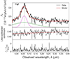 |
Fig. 1. Spectral line profile of the Paβ line. Top panel: Observed Paβ line profile (black) from MIRI MRS channel 1, extracted within a 3-kpc radius. The red line corresponds to our best-fit model (red). The two individual Gaussian components are displayed on the bottom as green and magenta dashed lines (offset from zero by an arbitrary amount). We mask a noise spike (shown in grey) shortwards of the line. Middle panel: Continuum after multi-Gaussian line subtraction. Bottom panel: χ statistic corresponding to the residuals between the model and the observed spectral profile, divided by the rms error in the continuum. |
The Hβ fit in Fig. 3 is complex as the line is blended with the [O III] doublet. For these three lines, as well as the He II line, in our model, we first included one component that is kinematically coupled in all lines (i.e. sharing the same velocity dispersion and velocity shift with respect to the rest-frame emission for all lines), corresponding to the extended narrow-line region. To account for outflows, we add a second narrow component which is blue-shifted and also tied in all lines (but independent of the first component). The [O III] doublet is fixed to a 1:3 flux ratio. Third, we add a broad component to Hβ for the BLR emission, which is independent of its kinematics. Finally, we can see that the underlying continuum is significantly affected by contribution from the low-ionisation Fe II complex, consisting of hundreds of velocity-broadened lines that altogether produce a pseudo-continuum. We used the optical Fe II template by Vestergaard & Wilkes (2001), convolved to the spectral resolution of the NIRSpec data and we applied a velocity broadening of 6000 km/s to it, which we experimentally determined to produce the best fit to the continuum shape upon visual inspection. In the middle panel of Fig. 3, we dissect the best fit of the line-subtracted continuum (red) into a linear component (orange dashed line) and the recovered Fe II contribution (blue dashed line).
The Hα line in Fig. 2 appears to be blended with [N II] from the narrow-line region. We modelled the narrow line contribution in Hα, [N II] and [S II] with two components (per line) fixed in their central wavelengths and widths to the narrow-line kinematics retrieved for the Hβ fit. The [N II] and [S II] components are shown as dotted lines, whereas the components belonging to Hα are marked by dashed lines. To the Hα fit, we add two broad components. The [N II] doublet is fixed to a 1:3 flux ratio. We note that the [N II] and [S II] contributions are very low, with an inferred [S II]/Hα flux ratio of 0.05 (similar to the low central values for the narrow component “Fc1” in Fig. 5 of Vayner et al. 2023).
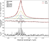 |
Fig. 2. Same as Fig. 1, but for the Hα line covered by our NIRSpec observations. The Hα kinematic components are shown as dashed lines, while the (weak) dotted Gaussians correspond to [N II] and [S II]. |
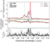 |
Fig. 3. Same as Fig. 1, but for the Hβ line covered by our NIRSpec observations. The dashed blue line in the middle panel shows the recovered contribution by the Fe II complex to the continuum, and the orange line is a linear fit to the residual continuum. The [O III] and He II lines are also covered, but not used in our analysis. |
In Fig. 4, we show the fit to the Mg II doublet in the rest-frame UV taken from the existing GNIRS observations (described in Section 2.2). Shortwards of the Mg II complex, there is a region affected by absorption (shown in grey in the top panel), which was masked for the fitting. We used two kinematic components to model each of the two Mg II lines, which we tied together in their fluxes by imposing a ratio of 1, assuming optically thick emission (Marziani et al. 2013). Similarly to the Hβ profile, the continuum is affected by Fe II emission, which we modelled by applying a 6000 km/s broadening to the UV Fe II template from the PyQSOFit (Guo et al. 2018) code, constructed by Shen et al. (2019) as a composite of the templates by Vestergaard & Wilkes (2001), Tsuzuki et al. (2006) and Salviander et al. (2007). In the middle panel of Fig. 4, we show the decomposed line-subtracted continuum into the inferred Fe II contribution (blue dashed line) and a linear fit (orange dashed line).
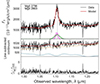 |
Fig. 4. Same as Fig. 1, but for the Mg II line covered by existing GNIRS observations. The dashed blue line in the middle panel shows the recovered contribution by the Fe II complex to the continuum. |
Table 1 contains the values of the recovered fit parameters. For any given line (Columns 1–2), we list the fitting parameters for individual Gaussian components and for the overall fit. The central velocity offset is given with respect to the rest-frame emission assuming z = 2.948 (Column 5). The next two columns list the integrated flux without any extragalactic extinction correction, and the associated rms-based signal-to-noise ratio (S/N; evaluated within ±2σ around the line and component). The final column corresponds to the dust-corrected integrated flux. The errors are inferred from from the covariance matrix estimated by lmfit, and in the case of the FWHM and the central velocity, we assumed a minimum error of 100 km/s to mitigate under-estimation. All fluxes listed in the table are corrected for Galactic extinction using the Schlafly & Finkbeiner (2011) dust maps and the Gaskell et al. (2004) AGN reddening law with a total-to-selective extinction ratio of 5.15 (Gaskell et al. 2004), except for the Paβ line which is shifted to the mid-IR. In the case of Mg II, we display the average over the two lines of the doublet (which were tied to have the same flux). The FWHM of the total profile is broadly similar for Paβ and Hα, at the level of ∼3700 − 3800 km/s while the Mg II profile is somewhat more narrow (∼3100 km/s) and that of Hβ broader (∼4300 km/s), though the width and central velocity of individual components can vary substantially. In particular, the Balmer lines contain a narrow component with FWHM ≲ 1500 km/s, while component 1 of the Paβ fit and component 2 of the Balmer lines are ambiguous with 2000 < FWHM < 3000 km/s. Table 1 and the comparison of Figures 1 and 2 also reflect that the Paβ line is intrinsically much fainter than Hα.
Results of the multi-component line fitting.
2.4. Virial BH masses
In this work, we compare the virial BH mass estimates obtained by using the kinematics of the Paβ line from our MIRI Ch1 observations. We also used the Hα and Hβ lines from our NIRSpec data and Mg II from existing GNIRS data.
The technique of virial BH mass estimates follows from the assumption that the motion of gas (or stars) in the close vicinity of a massive compact object can be used as a tracer of the enclosed mass. If the motions are virialised, the BH mass directly relates to the radius RBLR of the broad line region (BLR) and the velocity vBLR of the BLR gas (MBH = RBLRvBLR2/G). In the absence of reverberation-mapped BLR size measurements (Peterson 1993), BH masses can be estimated from calibrations based on strong lines (Kaspi et al. 2000), with RBLR and vBLR being traced by the luminosity Lλ and line width (e.g. full width half maximum FWHM), respectively:
In the above functional form, the virial scale factor, f, is a dimensionless parameter used to account for the (unknown) structure, dynamics and inclination of the BLR, and a and b are free parameters (with b being close to 2) fitted in reverberation mapping studies. We define the virial factor for the case of evaluating the line width via the FWHM, but we note that it would change if using the Gaussian velocity dispersion σ instead (see e.g. Onken et al. 2004; Woo et al. 2010; Park et al. 2012; Grier et al. 2013). In practice, the virial factor is inferred by matching the BH masses recovered by reverberation mapping to recover, on average, the MBH–σ⋆ relation. In nearby type 1 AGNs, Woo et al. (2015) found an average value of f = 1, while in reality f is likely to differ on a galaxy-to-galaxy basis and may depend on inclination, morphology (Ho & Kim 2014; Reines & Volonteri 2015), and the BLR velocity itself (Mejía-Restrepo et al. 2017). In this work, we explore both re-scaling all multi-wavelength virial MBH to a universal value of f = 1 following Mejía-Restrepo et al. (2022), as well as allowing f to be wavelength-dependent.
To estimate a BH mass for J1652 from the Paβ line, we follow the calibration from La Franca et al. (2015), which assumes a virial factor f = 4.31:
![$$ \begin{aligned} \log \frac{M_{\rm BH, \ \mathrm{Pa}\beta }}{M_\odot } &= (0.908 \pm 0.06) \cdot \log \left[ \left(\frac{{L_{\mathrm{Pa}\beta }}}{10^{40}\,\mathrm{erg/s}}\right)^{0.5} \ \left(\frac{\mathrm{FWHM_{\mathrm{Pa}\beta }}}{10^4\,\mathrm{km/s}}\right)^2 \right] \nonumber \\& \quad + (7.834 \pm 0.031). \end{aligned} $$](/articles/aa/full_html/2025/01/aa50451-24/aa50451-24-eq2.gif)
For the Balmer lines, we follow Eqs. (6) and (7) from Greene & Ho (2005):


where LHα, Hβ is the luminosity and FWHMHα, Hβ the FWHM of the respective line. To evaluate the line width, Greene & Ho (2005) and Mejía-Restrepo et al. (2022) used the broad component ascribed to the BLR (yielded by multi-Gaussian fitting). We iterate that the size of the BLR does not only depend on the luminosity, but can also be affected by the accretion rate of the quasar. Du & Wang (2019) have established a correction based on using Fe II/Hβ as a tracer of the Eddington ratio:
where RHβ,𠀄corr/uncorr denotes the corrected/uncorrected size of the BLR as inferred by Hβ, FFe II is the Fe II flux between 4434 and 4684 Å, and FHβ is the Hβ line flux. In our case, the correction is negligible, as we will discuss in more detail in Section 3.1.
For the Mg II-based constraint, we apply the calibration from Le et al. (2020) (Table 2, Scheme 2):
using their quoted rms scatter of 0.22 dex. The authors evaluated the FWHM from the full line profile without subtracting any subdominant narrow component. In all fits, we explore both measuring the width based on the total profile or only the broadest component yielded by our fit, to contrast the extreme cases. In the case of Mg II, we take the width and flux of a single line from the doublet.
2.5. SED fitting procedure
We used the SED fitting Code Investigating GALaxy Emission (CIGALE) (Boquien et al. 2019) to constrain the stellar mass of J1652, combining the JWST observations with ancillary UV-to-IR photometry. To construct the SED of J1652, we started with the existing SDSS data in the ugriz filters. We add JWST/NIRSpec and JWST/MIRI observations, extracting narrow-band images within a 3 arcsec diameter, centered on 2.2, 2.9, 5.235, 8.2, 12.5, and 19.6 micron (within the stellar continuum). We added the W1 to W4 filters (at 3.4, 4.6, 12 and 22 micron) from the Wide-field Infrared Survey Explorer (WISE; Wright et al. 2010), extracted within 3 arcsec diameter, as well as an upper limit in the E-band (217 μm) from the Stratospheric Observatory For Infrared Astronomy (SOFIA; Miles et al. 2013). The full SED is shown in Fig. 5, with the SOFIA upper limit falling outside the y-axis range. The consistency between the 12 micron WISE W3 flux and the MIRI MRS Ch3 mock photometry at 12.5 micron suggests that the MIRI data is not affected by any severe flux calibration issues. We note that channel 4 is known to be affected by a time-dependent loss of sensitivity, for which the data reduction pipeline includes a correction. The Paβ line falls into channel 1 of the MIRI MRS observations.
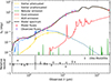 |
Fig. 5. SED fit obtained for J1652 with the CIGALE code. The observed photometry is displayed by violet circles, and model fluxes are shown as red dots, while the black curve corresponds to the model spectrum. The different components included in the fit are: dust emission (red), AGN template (orange), nebular emission lines (green), and the host galaxy contribution (shown in blue and yellow, with and without dust attenuation, respectively). |
We ran CIGALE with the following settings: We used the Bruzual & Charlot (2003) library, and parametrise the star formation history via the “sfhdelayed" model, corresponding to a delayed rise of the SFR up to a maximum, followed by an exponential decrease in cosmic time. We used an e-folding time of 110 Myr and imposed an upper limit of 1 Gyr on the age at z = 3, which was chosen as the best fit (lower limit: 100 Myr). We allowed for an optional decoupled burst amounting to a mass fraction of ≤10%, but it is not used in the best fit. For the AGN component, we used a template from the SKIRTOR database (Stalevski 2012; Stalevski et al. 2016) and retrieved the following best-fit parameters: t = 3 (optical depth at 9.7 micron), p = 1 (power-law exponent), q = 1.5 (index for dust density gradient), oa = 80° (opening angle), R = 30 (outer-to-inner radius ratio), and i = 10° (inclination). We used a fixed fraction of dust in clumps Mcl = 0.97 and an emissivity of 1.6. For the dust attenuation settings, we assumed the Gaskell et al. (2004) AGN extinction law. We leave the attenuation E(B−V) to vary between 0.28–0.34 informed by our measured Balmer decrement, with a best-fit value of 0.3, and no reduction for the continuum attenuation (while our settings allowed a reduction by ≤30%). We used a Salpeter (1955) initial mass function. The dust emission is following Draine et al. (2014). The nebular emission lines were modelled self-consistently with a CLOUDY (Ferland et al. 2017) photoionisation model grid generated by Inoue (2011). Our best fit model exhibits a low metallicity of 0.0004 for gas and stars alike. We present the SED fit in Fig. 5. The under-prediction at 5 micron in the SDSS g band may stem from the Lyα emission not being accurately captured, as Lyα may not be confined to the host galaxy itself, but can occur on extended scales (e.g. Daddi et al. 2021). Indeed the Lyα line in the SDSS spectrum is strong, with a flux exceeding the CIGALE prediction roughly by ∼0.01 mJy.
3. Results
In this section, we compare the broad line profiles, calculate virial BH mass estimates and Eddington ratio constraints from the Mg II, Hα, Hβ and Paβ emission. We set the resulting constraints into the context of the MBH–M⋆ relation alongside other high-redshift AGN populations.
3.1. Broad line properties and BH mass estimates
In the left panel of Fig. 6, we compare the spectral line profiles of Paβ (red) and Hα (black) in velocity space. We omit Hβ and Mg II because of their strong blending (see Figs. 3 and 4). The Paβ profile is clearly much noisier than Hα (which introduces additional uncertainty in the recovery of its broad component), but at first glance, there is an excellent match between the two profiles, with no obvious velocity dependence of the Paβ /Hα ratio. The agreement between Hα and Paβ linewidths is consistent with findings for local X-ay selected AGNs from the BAT (Burst Alert Telescope) AGN Spectroscopic Survey (BASS) survey (Lamperti et al. 2017). We interpret the observed similarity and the broad width in profiles as an indication that the broad emission indeed stems from the BLR. In the right panel, we overplot our best-fit model profiles obtained via summed Gaussians (see Section 2.3) for Paβ (red), Hα (black) Hβ (grey), and Mg II (blue) in a normalised fashion. The horizontal dashed line denotes the 50% flux level at which the FWHM is evaluated. The broad components of the different line profiles deviate somewhat, with Hβ exhibiting a notable redshifted broad component which may be affected by blending. The origin of the redshift is not obvious, since the broad components of both Balmer lines should originate from the same BLR gas. We checked that refitting the Hβ profile while tying the central wavelength offset of the broadest component to that of Hα does not lead to a good fit, as we show in Appendix A (Fig. A.1). However, the FWHM of the four summed profiles is remarkably similar (see Table 1 for the exact parameter values). However, as mentioned in Section 2.3, the relative strength, width and central velocity of individual components can vary significantly, and the assignment to a broad/narrow component can be considered ambiguous for both component 1 of the Paβ fit and component 2 of the Balmer lines (2000 < FWHM < 3000 km/s). We therefore contrast the extreme cases – deriving BH masses based on the broadest kinematic component only, or alternatively based on the width of the full line profile.
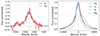 |
Fig. 6. Comparison of line profiles. Left panel: Superposition of the Paβ (red) and Hα (black) line profiles in velocity space. The fluxes are in arbitrary units. There is a close match in the total line profiles, with the peaks (set by the narrow component) occurring at similar velocities assuming a redshift of z = 2.94. We omit the Hβ and Mg II profiles from this panel since they are strongly blended, but they can be seen in Figs. 3 and 4. The features shortwards of ∼ − 5000 km/s in the Paβ profile are masked in the fitting. Right panel: Superposition of the total line profiles of Paβ (red), Hα (black), Hβ (grey) and Mg II (blue) as recovered by our multi-Gaussian line fitting procedure (arbitrary flux units). |
We apply a dust attenuation correction based on the Balmer decrement. We assume an intrinsic Hα/Hβ ratio of 3.1 for AGNs, which is typically assumed in the case of the narrow-line region (Halpern & Steiner 1983), while for the BLR, different studies find a large span in Hα/Hβ ratios ranging between 2.5–6.6 (Ward et al. 1988; Dong et al. 2008; Schnorr- Müller et al. 2016; Gaskell 2017). The intrinsic ratio can vary in the BLR. Using the Gaskell et al. (2004) AGN extinction curve and a total-to-selective extinction ratio of 5.15 (Gaskell et al. 2004), we recover a V-band attenuation of AV = 0.85 mag. We derive an alternative attenuation from the Paβ/Hα decrement, leading to AV = 0.54 − 0.87 mag if assuming an intrinsic Hα/Paβ ratio of 10 or 12. Kim et al. (2010) derive a mean Hα/Paβ ratio of ∼10 in type 1 AGNs, which the authors show to be broadly consistent with Case B recombination (optically thick to ionising photons produced by recombination) for a BLR density of n = 109 cm−3 when exploring a range of ionisation conditions and densities. The exact value can vary, for instance Hα/Paβ ∼ 17 for a temperature of 104 K and a hydrogen density of 1010 cm−3 in the reference table of Hummer & Storey (1987). Henceforth, we choose to correct for extinction based on the Balmer decrement. Our dust-corrected flux measurements are listed in the last column of Table 1.
With dust-corrected line fluxes in hand, we can derive virial BH mass estimates according to Eqs. (2), (3), and (4), with varying assumptions. One of the uncertainties in the method stems from the discrimination between broad and narrow components being ambiguous in some cases (see the components with 2000 < FWHM < 3000 km/s in Table 1). We therefore explore both using the FWHM of the broadest component and that of the total line profile, to contrast the extreme cases. The resulting spread of BH masses is summarised in Fig. 7, with the four sections displaying Paβ-, Hα-, Hβ- and Mg II-based estimates, respectively. We first explore re-scaling all calibrations to a virial factor f = 1 (left panel), under the assumption that the structure and geometry of the BLR remain consistent across all wavelengths. We repeat the exercise allowing for a wavelength-dependent f factor, taken from the original calibrations (right panel). For each line, we derive four estimates as specified by the y-axis labels: based either on using the total line profile (circles) or alternatively using the FWHM and luminosity of the broadest component only (diamond symbols), and in each case adopting either the observed luminosity (open circle) or the dust-corrected one (filled circle). We display the median among all constraints as a solid vertical line (log MBH = 9.4 if setting f = 1, 9.6 otherwise), with the shading indicating the ±1 standard deviation. In the right panel, we add four open rectangles to highlight the treatment from the original calibrations. The vertical dashed line denotes the constraint from Perrotta et al. (2019), who used the galaxy-integrated Hβ line from Gemini/GNIRS data (dust-corrected via the extinction derived from the r, i, z − W1 colours in Hamann et al. 2017), which falls between all of our Hβ-based estimates. The errorbars on the points are deliberately chosen to display only the quoted scatters in Equations (2), (3) and (4) and a ∼30% uncertainty on the virial factor f (Woo et al. 2015), which visibly fails to span the full range of BH mass estimates for our rapidly accreting, extremely red quasar which harbours strong outflows.
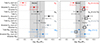 |
Fig. 7. Spread in virial BH mass estimates for J1652 recovered from the kinematics of different broad lines (Paβ: red symbols, Hα: black symbols, Hβ: grey symbols, Mg II: blue symbols) under varying assumptions, as specified by the labels on the y-axis. In the left panel, we rescaled all virial BH masses to a common virial factor f = 1, while in the right panel the original f values from the calibrations are applied (f = 4.31 for Paβ, f = 0.75 for the Balmer lines and f = 1 for Mg II). For each line, we show the mass recovered by using the total line profile (circles) versus the broadest component of our line fit only (diamonds), and observed fluxes (open circles) versus dust-corrected ones assuming AV = 0.89 mag (filled circles). The individual errorbars reflect the uncertainties quoted in the coefficients of the virial mass prescriptions (Eqs. (2), (3), and (4)), and we caution that they do not cover the range of BH masses obtained with our different assumptions for J1652. The vertical dashed line indicates the BH mass constraint by Perrotta et al. (2019) based on the galaxy-integrated Hβ emission in Gemini/GNIRS observations. The median log MBH among all of our estimates is indicated by the solid vertical line, with the shaded region corresponding to ±1 standard deviation. With four open rectangles, we highlight the treatment from the original calibrations in the right panel. |
The Balmer-based MBH estimates alone span ∼1.5 dex with errorbars. Despite the different ionisation potential of the Mg II line, the UV-based estimates are consistent with the constraints given by the Hα and Hβ lines. However, when requiring a uniform virial factor, the Paβ-based constraints fall notably below the other estimates. This is unexpected, given that the Paschen and Balmer lines trace the same ionised hydrogen. This may be in part due to the faintness of the Paβ emission, which renders it challenging to constrain the broad component in the line profile, both in our observations and in the literature. Further, there exist fewer literature datasets of Paβ observations than for the Balmer lines, which may affect the robustness of the derived virial calibrations (with a sample size of 16 AGNs for the La Franca et al. (2015) calibration, compared to 229 in Greene & Ho 2005). However, allowing for a wavelength-dependent virial factor f also alleviates the tension. This is in agreement with results on low-redshift X-ray AGNs studied by Lamperti et al. (2017), who found their Paβ-based BH masses derived with f = 4.31 to be consistent with Hβ-based estimates derived with f = 1 from the BAT AGN spectroscopic survey (Koss et al. 2017).
Arguably, choosing the broadest component to derive the BH mass lacks physical significance, as the distinction of which components are or aren’t part of the BLR remains unclear. However, even if focusing only on estimates derived via the total profile, the spread is still ≳1 dex with uncertainties. We note that all of the lines in our data come with their own benefits and disadvantages: While the Hα line has the highest S/N, the BH mass based on the total Hα profile is affected by blending with the [N II] doublet. Hβ and Mg II are strongly blended and more sensitive to dust extinction. Paβ is less dust-sensitive, but fainter.
Our large span in recovered BH masses highlights that the virial approach can be very fraught. For instance, the BLR gas may not satisfy virial equilibrium conditions, especially in J1652 given the presence of a powerful outflow and near-Eddington accretion (Zakamska et al. 2019). Also, dual AGNs resulting from a merger may host two broad-line regions, leading to double-peaked or unresolved broad lines (Kim et al. 2020). As mentioned before, the virial scale factor f can vary substantially between different AGNs based on the geometry, structure and inclination of the BLR. Moreover, the size of the BLR as inferred from the observed luminosity at optical/NIR wavelengths depends on the assumptions about dust correction, which is particularly relevant in the dust-rich centres of ERQs. In this work, we use the Balmer decrement and assume the Gaskell et al. (2004) dust law to correct for extinction. Observational uncertainties include sensitivity issues which may lead to missing a faint broad component, ambiguity in the assignment of broad/narrow components and strongly blended line profiles (all of which are relevant for our observations).
We also note that in the case of Hβ, we used Eq. (6) to attempt to correct the inferred BLR size for the Eddington ratio according to the prescription by Du & Wang (2019), which traces the accretion rate via the Fe II/Hβ flux ratio. The latter amounts to ∼0.33 for our fit. However, the inferred corrective factor is small (0.1 dex), and we thus omit it. Finally, as an experiment, we tried using the C IV line from the SDSS spectrum as a kinematic tracer. Using the calibration from Vestergaard & Peterson (2006) (with f = 1), we retrieved a constraint of log M = 8.4 − 8.7, which we omit from Fig. 7 since C IV-based BH masses are known to be subject to particularly large uncertainties as the C IV line profile may be dominated by non-gravitational effects (Baskin & Laor 2005). Zakamska & Alexandroff (2023) moreover demonstrated via a spectropolarimetric analysis that the rest-frame UV broad-line region in J1652 is strongly affected by outflows and reprocessing.
3.2. Stellar mass of J1652
In the absence of sufficient wavelength coverage, galaxy masses are typically constrained by probing their luminosity and assuming a mass-to-light ratio. Applying this approach to J1652, based on direct Hubble Space Telescope (HST) imaging, yields a broad stellar mass estimate in the range of log M⋆/M⊙ = 11.4 − 12.4 (Zakamska et al. 2019), assuming a mass-to-light ratio of 0.4 − 4 M⊙/L⊙ for a stellar population aged 0.3–2 Gyr (Maraston 2005) and correcting from the B-band to the bolometric luminosity. However, the inferred luminosity depends on the assumptions on dust obscuration and AGN contribution, and the mass-to-light ratio M/L is known to vary substantially on a galaxy-to-galaxy basis (see e.g. van de Sande et al. 2015 recovering M/L spreads of 1.6/1.3 dex in the g/K band for a sample of massive quiescent galaxies out to z = 2). Given the availability of multi-band imaging or spectroscopy, an alternative approach lies in modelling the SED or spectrum.
Based on UV-to-IR SED fitting as outlined in Section 2.5, we retrieve a remarkably large stellar mass for J1652 of log M⋆/M⊙ ∼ 12.1 M⊙, consistent with the previous constraint. We caution that J1652 is dominated by the AGN component, as can also be seen in the best fit shown in Fig. 5. As a result, the uncertainties on the stellar mass are exacerbated. Our best-fit model has χ2 = 5.0. We estimate the uncertainties on the stellar mass by going through the grid of CIGALE models, selecting those with a similar χ2 (within 5 percent), and retrieving the associated stellar masses. This approach leads to a broad range of estimates spanning 11.5 < log M⋆/M⊙ < 12.6, highlighting the weak constraint on the host. The scale of the uncertainty is similar to that quoted by Narayanan et al. (2024) at higher redshift, who found that different SED fitting codes can diverge in their predicted stellar masses by ∼1 dex even in the case of non-AGN galaxies. In Fig. 5, the observed photometry of J1652 is shown as violet circles, with the best-fit model overplotted (red dots = model photometry, black curve = model spectrum). The reprocessed dust emission is shown in red, the AGN component in orange, and the attenuated/unattenuated stellar contribution in yellow/blue. The datapoints from MIRI Ch4 and WISE W4 are somewhat under-predicted, which could be due to the underlying assumptions on polycyclic amoratic hydrocarbons (PAH) templates, dust extinction law, or AGN templates, as well as MIRI Ch4 being affected by time-dependent loss of sensitivity and thus relying on a correction to the flux calibration. The fit quality is encouraging in the optical and UV, which are most sensitive to the stellar mass. In any case however, we iterate that the uncertainties involved in fitting the SED of an extremely luminous quasar at high redshift are large.
According to our best fit, J1652 is thus placed at the extreme end of the z = 3 galaxy stellar mass function, namely > 1 dex above the characteristic mass of the Schechter fit (Leja et al. 2020), though we note again the large uncertainties involved. As a result, J1652 is an exceptional target even among extremely red quasars, which are known to reside in massive galaxies (Zakamska et al. 2019). Remarkably, J1652 furthermore has three close spectroscopically confirmed companions (all at projected distances < 15 kpc) which among themselves span a velocity range of ∼1000 km/s, and existing HST images reveal indications of a larger-scale overdensity (Wylezalek et al. 2022). These observations suggest that J1652 is potentially residing at the core of a forming protocluster at z = 3, which may have contributed to its rapid mass build-up.
3.3. J1652 in the context of the BH mass–stellar mass relation
In Fig. 8, we place J1652 on the local MBH–M⋆ relation from Reines & Volonteri (2015) (blue solid line with associated scatter shown by the shaded region). We also display the local relation from Kormendy & Ho (2013) for elliptical galaxies (dashed blue line), assuming their bulge mass corresponds to the total stellar mass, to show the dependency of the local relation on morphology. As an indication of the dynamic mass range of the established relations, we grey out the region that is extrapolated beyond the low-redshift datapoints (log M⋆ ≲ 11.5 for Reines & Volonteri (2015), ≲12.1 for the ellipticals in Kormendy & Ho 2013). The grey vertical bar indicates the ±1σ spread around our median recovered BH mass of log MBH = 9.6 assuming a wavelength-dependent virial factor f (grey shaded region in the right panel in Fig. 7), with the white and yellow diamond symbols showing the extreme cases (based on the total Paβ profile without dust correction and broadest Hα component with extinction-corrected flux, respectively). The thin vertical arrow includes the errorbars quoted in Eqs. (2) and (3). From the range of stellar masses spanned by viable models in our SED fitting procedure, we infer an estimated uncertainty of 1 dex (see Section 3.2). This is similar to the spread Narayanan et al. (2024) recover when comparing the outcome of different SED fitting codes at high redshift. We caution that the difficulty of conducting AGN-host decompositions in luminous quasars may yet increase the errorbars in our case, and the SED shape may be impacted by scattered light from the quasar. It is a sobering assessment that, depending on the line used as a tracer and the underlying assumptions as well as given the uncertainties, J1652 could be interpreted as being highly overmassive or at a typical mass for its host, relative to the extrapolated Reines & Volonteri (2015) relation. With a Sérsic index of ∼3.4 (Zakamska et al. 2019), J1652 corresponds to an intermediate morphological type and may thus be expected to reside above the Reines & Volonteri (2015) relation for all galaxy types, approaching instead the relation for elliptical galaxies. For context, we also overplot two other quasar populations at Cosmic Noon from the literature, namely high-redshift radio galaxies (HzRGs) from De Breuck et al. (2010) and Nesvadba et al. (2011) (green squares; z ∼ 2) which are known to reside in massive, bulge-dominated hosts, and a sample of X-ray detected broad-line AGNs at z ∼ 1.5 (Suh et al. 2020) which includes several massive sources exceeding 1012 M⊙. Across this compilation of literature quasar samples, J1652 is among the most massive galaxies. In the Faint Images of the Radio Sky at Twenty Centimeters (FIRST; Becker et al. 1995) survey, J1652 is detected as an unresolved radio source (Hwang et al. 2018), without any evidence for extended radio jets.
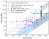 |
Fig. 8. Our range of recovered BH mass estimates for J1652 (grey bar) in the context of the low-redshift MBH–M⋆ relation for all broad-line AGNs (blue solid line; Reines & Volonteri 2015) and for ellipticals with suppressed star formation (blue solid line; Kormendy & Ho 2013). Depending on the choice of line (Paβ, Hα, Hβ, and Mg II) and underlying assumptions (assignment of kinematic components to the broad line region, virial factor, f, dust attenuation, etc.), and considering the uncertainties, one could argue that J1652 is overmassive or falls onto the MBH–M⋆ relation. The uncertainty on the stellar mass is derived from considering all SED models explored with a similar goodness of fit (χ2 within 5% of the best fit value). For context, we add a sample of massive high-redshift radio galaxies (green squares; De Breuck et al. 2010; Nesvadba et al. 2011), and unobscured X-ray AGNs at Cosmic Noon (purple circles; Suh et al. 2020). |
3.4. Eddington ratio of J1652
J1652 is likely a near-/super-Eddington accreting source, as shown by Zakamska et al. (2019). We propagate the uncertainties in our BH mass estimates to a spread of inferred Eddington ratio constraints. The bolometric luminosity of J1652 based on either [O III] or WISE photometry was estimated to amount to ∼1047 − 48 erg/s by Perrotta et al. (2019), Ishikawa et al. (2021). Based on the galaxy-integrated Hβ -based BH mass, these authors also derived a rough estimate of the Eddington ratio consistent with super-Eddington accretion at the level of ∼1.2. We note that there are significant uncertainties in the inferred bolometric luminosity when comparing multi-wavelength bolometric corrections, based on e.g. the [O III] line flux (Reyes et al. 2008) or the 3.45 μm near-IR luminosity (Lau et al. 2022). As a result, bolometric luminosity constraints can disagree by 1–2 dex or more (see also Wang et al. 2023a), especially in the case of dust-reddened systems that require an extinction correction.
Assuming a bolometric luminosity of 5 × 1047 erg/s, we recover an Eddington ratio of > 20% (> 10% with errorbars) even in the case of our highest recovered BH mass of log MBH = 10.1 (∼10.5 with errorbars). Our lower MBH estimates suggest possibly highly super-Eddington accretion, which could contribute to the large uncertainties as the BLR gas may not be virialised in this regime. Even with the most conservative estimates though, we recover an Eddington ratio substantially larger than 1%, below which the accretion flow would be radiatively inefficient (Xie & Yuan 2012; their Fig. 1). Assuming Eddington accretion motivated by the findings of Zakamska et al. (2019) would place the BH mass in the range of 108.9 − 9.9 M⊙, which is exceeded by our Hα-based MBH constraints inferred from the broadest component only. This is a further argument against using the broadest component, which depends on the particular settings of the fitting procedure and is not physically meaningful.
The Fe II/Hβ flux ratio may also be used as a tracer of the Eddington ratio (e.g. Boroson & Green 1992; Du & Wang 2019). When measuring between 4400 and 4800 Å, we obtain a flux ratio of 0.33, which corresponds to an Eddington ratio of ∼40% (Gaskell et al. 2022; Fig. 12), consistent with our range of estimates.
4. Discussion of BH mass studies at high redshift
The advent of the JWST has brought to light a substantial number of overmassive BH candidates at high redshifts ≳4, potentially suggesting a strong redshift evolution of the stellar mass–BH mass relation at the earliest cosmic times. In principle, these analyses can yield valuable information about the prevalence of different BH seeding and growth mechanisms.
However, at high redshift, the determination of BH masses relies heavily on single-epoch virial calibrations, of which there exist numerous different prescriptions – which were all established at low redshift, although we refer the reader to Abuter et al. (2024) for a recent dynamical mass constraint in a z = 2.3 AGN. In general however, it is unclear whether single-epoch virial calibrations are applicable to the high-redshift Universe, but cross-calibrations with other methods are difficult to conceive of. In the case of rapid accretion, or in the presence of turbulent gas and outflows, the assumption of virial equilibrium may not hold. At z = 0.4, Fries et al. (2024) recently presented a case of a highly non-virialised BLR as inferred by reverberation mapping over 10 years. The assembly of quasars at high redshift is still a matter of debate, and luminous quasars could potentially have undergone (super-)Eddington accretion, which would disturb the virial equilibrium (e.g. King 2024). Further, the fraction of AGNs with extreme outflows seems to increase with redshift out to z ∼ 6 (Bischetti et al. 2022). Virial BH masses can moreover be subject to observational effects, such as missing a faint broad component due to a lack of sensitivity, blending of lines, or not resolving dual AGNs (e.g. Liu et al. 2018).
Besides these limitations, there are a number of methodological differences among the virial calibrations themselves. We illustrate this point with Table 2, in which we compile an overview of several recent literature studies at the highest redshifts with their choices of calibration and methodological details. Choices of assumptions include the adopted value for the virial factor f (accounting for the geometry of the BLR), whether a dust correction is applied to the luminosity tracing the BLR size, whether the host galaxy contribution is subtracted, and how the line width is defined for tracing the velocity of BLR clouds (FWHM of the total line profile, or the recovered broad component). Table 2 is split in three parts, corresponding to studies finding evidence for overmassive BHs compared to the local stellar mass–BH mass relation, mixed results, or samples consistent with local host scaling relations. It can be appreciated that there is a large variety of approaches used across the community. Different calibrations use virial factors differing by a factor ∼5. At z = 6, dust extinction in individual galaxies could still reach AV values as large as ∼1 (Schaerer & de Barros 2010), such that Mg II-based BH mass estimates could be under-predicted by a factor ∼2 if no dust correction is implemented. In J1652, the recovered BH mass moreover changed by a factor ∼4 on average depending on whether a given calibration was applied using either the full line profile or the broadest component. Thus, the range of methods used in the literature alone leads to a significant systematic uncertainty.
Overview of various literature studies on SMBH masses MBH at high redshift.
While the majority of analyses in Table 2 support overmassive BHs at high redshift at first glance, observational biases may play a strong role, e.g. in preferentially selecting the most luminous quasars, which are to first order powered by the most massive BHs (Lauer et al. 2007). Pacucci et al. (2023) argue that the JWST flux limits should not prevent the detection of lower-mass BHs in surveys such as CEERS (Cosmic Evolution Early Release Science survey; Finkelstein et al. 2023) and JADES (JWST Advanced Deep Extragalactic Survey; Eisenstein et al. 2023), as a BH weighing 106.2 M⊙ should still produce a Hα BLR measurable at the 3σ-level. On the other hand, the fraction of unobscured broad-line AGNs exhibiting broad lines itself may be BH mass-dependent (Schulze & Wisotzki 2011; Li et al. 2024). Stone et al. (2024) instead construct a mock biased sample of luminous low-z AGNs, mimicking the selection effects of their z > 5 sample, with the caveat that the low-z population may deviate from the high-z one in properties such as the Eddington ratio distribution function. They infer a mock biased local MBH–M⋆ relation, which is significantly offset from their five high-z quasar constraints. In any case, studies of ‘typical’ AGNs at high redshift are sparse. One relevant initiative is the SHELLQs project (Subaru High-z Exploration of Low-Luminosity Quasars; Matsuoka et al. 2016) identifying low-luminosity quasars at z ∼ 6 via photometric colour cuts in the wide-field Subaru HSC-SSP survey (Hyper Suprime-Cam Subaru Strategic Program; Aihara et al. 2022). For those SHELLQs AGNs with existing UV spectra, their Mg II – based BH masses are found to be broadly in line with local host galaxy scaling relations (Izumi et al. 2018, 2019, 2021). Due to the absence of stellar mass constraints, the dynamical mass (from [C II] measurements) was equated to the bulge stellar mass, which may as a result be overestimated, given the gas-rich character of high-redshift galaxies. The studies of Pensabene et al. (2020) and Willott et al. (2017) instead placed high-z AGNs with [C II] measurements (including several lower-luminosity targets) on the BH mass-dynamical mass plane along with the local relation, yielding mixed results. Overall, distinct selection effects remain poorly characterised and merit dedicated follow-up investigations as number statistics grow.
Besides the selection effects limiting our view of the high-z AGN population, a further obstacle to studying the redshift evolution of the BH mass–stellar mass relation lies in the determination of stellar masses at high redshift, where galaxies are ≲1 Gyr old. Among young stellar populations of different ages, the stars formed in the most recent burst outshine the previous generations, even if they do not dominate the mass budget. Therefore, it is challenging to infer the total stellar mass via fitting the spectral energy distribution (SED). As a result of this limitation by nature, fitting procedures are highly sensitive to the assumed shape and priors of the star formation history and inferred stellar masses can vary by ∼1 dex even for non-AGNs (Narayanan et al. 2024). This is still less than the claim of a ∼2 dex excess in M⋆ w.r.t. the local MBH–M⋆ relation for high-z AGNs (Maiolino et al. 2024; Pacucci et al. 2023). However, the presence of an AGN constitutes a further complicating factor (see e.g. van Mierlo et al. 2023), as the SED needs to be decomposed into the individual AGN and host contributions.
Clearly, it is necessary to consider the cumulative impact of different selection biases and uncertainties. Combining data from deep JWST surveys, Li et al. (2024) statistically model the combined effects of sensitivity limits, a potentially mass-dependent fraction of broad-line AGNs, and uncertainties in the stellar mass and BH mass. The authors conclude that the recent observations of massive broad-line AGNs in JWST surveys are not inconsistent with the local MBH–M⋆ relation. Thus, the relation may evolve with redshift to produce overmassive BHs in the early Universe, or it could remain constant but exhibit a larger scatter at higher redshifts.
All things considered, it is imperative to continue expanding datasets of high-redshift AGNs to include lower-luminosity sources and increase number statistics, as well as to improve BH mass calibrations for targets at early cosmic times, or develop new techniques altogether (a particular challenge at high redshift). Using the SHELLQs dataset, Takahashi et al. (2024) explore assigning low-redshift counterparts to high-z AGNs to broadly constrain the latter’s BH masses via “spectral comparison”, with the limitation of being confined to the properties of low-redshift BHs, by definition. Reverberation mapping campaigns are branching into the high-redshift regime, with initiatives such as the SDSS-RM project containing several sources beyond z = 3 (Shen et al. 2024), though they are very time-consuming by nature (and relying on the assumption of virial equilibrium like single-epoch virial BH mass estimates). The technique of optical-UV continuum reverberation mapping (Netzer 2022) and relating the BLR size to the size of the continuuum emitting region (Wang et al. 2023b), presents a possible way to shorten the time requirements of observational campaigns in the landscape of upcoming time domain surveys. Further, there have been attempts to establish BH mass calibrations based on X-ray properties at low/intermediate redshift (e.g. Mayers et al. 2018; Akylas et al. 2022). Remarkably, at Cosmic noon, the GRAVITY+ collaboration recently dynamically measured the BH mass of an AGN at z = 2.3 by modelling the blue and red photocentres of the BLR via analysis of the differential phase curves of different baselines, suggesting an under-massive BH (Abuter et al. 2024).
Yet, in the foreseeable future, single-epoch virial BH mass constraints are certain to remain indispensable tools for studying the growth of BHs and their connection to their hosts at high redshift. To mitigate the sensitivity of inferred BLR sizes (and thus virial BH masses) to rapid gas accretion, Du & Wang (2019) established a correction to Hβ-based virial BH masses based on tracing the Eddington ratio via the Fe II-to-Hβ ratio. While this correction did not significantly change the results on J1652’s BH mass in this paper, it reduced the Hβ -inferred BH mass of the aforementioned GRAVITY+ target by ∼0.6 dex, leading to consistency with their dynamical mass measurement. Kuhn et al. (2024) recently presented a method that can constrain the virial factor in individual AGNs by dynamically modelling the BLR and simultaneously fitting a range of lines, while leaving as free parameters the radial distribution of BLR emitters at different wavelengths. It is also key to continue to identify and follow-up lower-luminosity AGNs (such as those from the SHELLQs project) in surveys that are both deep and wide. For instance, Greene et al. (2024) showed that the majority of the faint “Little Red Dots” (Matthee et al. 2024; Kokorev et al. 2024) identified in JWST/NIRCam surveys exhibit broad lines consistent with those seen in the broad-line region of AGNs, and proposed refined colour cuts to avoid contamination by brown dwarfs (Langeroodi & Hjorth 2023). However, Yue et al. (2024b) reported a non-detection when stacking X-ray observations of Little Red Dots, and inferred an upper limit ∼1 dex lower than expected based on the Hα emission, which suggests the population significantly differs from typical lower-redshift type-I AGNs. It is worth noting that at high redshift, AGN identification relies largely on the presence of broad lines due to the strong redshift evolution of narrow-line diagnostics such as the Baldwin et al. (1981) diagram (Kewley et al. 2013), though there are efforts to use high-ionisation lines instead (Scholtz et al. 2023). On the other hand, Kirkpatrick et al. (2023) find that colour cuts in JWST/MIRI photometric data alone do not effectively select AGNs, while machine learning algorithms may offer a valuable alternative in the future (see e.g. Tardugno Poleo et al. 2023). Gravitationally lensed systems may also offer opportunities to constrain the BH masses of fainter AGNs (Melo et al. 2023). In conclusion, the ongoing exploration of high-redshift AGNs in the JWST era underscores the importance of continuing to collect observations of different types of AGNs, but also refining and innovating our analytical tools.
5. Summary and conclusion
Based on JWST/NIRSpec and MIRI data, we present updated constraints on the stellar and BH mass of the extremely red quasar J1652, a system harbouring vigorous outflows and starbursting clumps, residing amidst three interacting companions. Our conclusions are as follows:
-
The spectral profiles of the Paβ, Hα, Hβ and Mg II emission are broadly similar in terms of total FWHM, but individual kinematic components differ in their width, velocity shift, and relative flux (Fig. 6, Table 1).
-
The recovered virial BH mass estimates for J1652 strongly depend on the choice of line and kinematic component(s), as well as on the choice of virial factor and slightly on the dust correction (Fig. 7). When allowing for a wavelength-dependent virial factor, the recovered estimates range from log MBH/M⊙ ∼ 9 (total Paβ profile) to 10.1 (broadest Hα component). Each of the lines explored has its advantages and drawbacks: Paβ is mostly insensitive to dust extinction, but intrinsically fainter than the Balmer lines. Hα is the strongest line, but blended with [N II] emission. Mg II and Hβ are the bluest and thus most dust-sensitive lines and significantly blended with Fe II. Hβ is also blended with [O III], but its profile still remains better resolved than the Hα-[N II] complex.
-
Based on UV-to-IR SED fitting with the CIGALE code (Boquien et al. 2019), we retrieved a stellar mass of
 , which places J1652 at the extreme end of the z = 3 galaxy stellar mass function. The uncertainties are large when fitting a strongly quasar-contaminated SED at high redshift.
 -
In the context of the BH mass–stellar mass relation, we caution that the choice of line, kinematic component(s), along with any other assumptions as well as the uncertainties in the stellar mass, can lead to assessing the BH in J1652 as over-massive or even typical for its host galaxy stellar mass.
-
However, even with our most conservative estimate, we obtained an Eddington ratio in excess of 10%, clearly exceeding the threshold below which the accretion is radiatively inefficient (Xie & Yuan 2012).
Our findings highlight the caveats associated with virial BH mass constraints, especially in the presence of a fast accretion flow and strong outflows at high redshift. We note that this work is a single-object study of a specific quasar phase, thus, it is essential to continue building larger samples to reduce the impact of individual uncertainties in statistical studies of the general population. At the same time, in light of the growing number of studies on high-redshift BH demographics in the era of the JWST, our results serve as a cautionary tale, underscoring the need for transparency about the uncertainties inherent to the method.
Acknowledgments
We thank the anonymous referee for helpful comments. D.W. and C.B. acknowledge support through an Emmy Noether Grant of the German Research Foundation, a stipend by the Daimler and Benz Foundation and a Verbundforschung grant by the German Space Agency. D.S.N.R., N.L.Z., and S.V. are supported by NASA through STScI grant JWST-ERS-01335. N.L.Z further acknowledges support by the Institute for Advanced Study through J. Robbert Oppenheimer Visiting Professorship and the Bershadsky Fund. J.B.-B. acknowledges support from the grant IA- 101522 (DGAPA-PAPIIT, UNAM) and funding from the CONACYT grant CF19-39578.
References
- Abuter, R., Allouche, F., Amorim, A., et al. 2024, Nature, 627, 281 [NASA ADS] [CrossRef] [Google Scholar]
- Aihara, H., AlSayyad, Y., Ando, M., et al. 2022, PASJ, 74, 247 [NASA ADS] [CrossRef] [Google Scholar]
- Akylas, A., Papadakis, I., & Georgakakis, A. 2022, A&A, 666, A127 [NASA ADS] [CrossRef] [EDP Sciences] [Google Scholar]
- Alexandroff, R. M., Zakamska, N. L., Barth, A. J., et al. 2018, MNRAS, 479, 4936 [NASA ADS] [CrossRef] [Google Scholar]
- Argyriou, I., Glasse, A., Law, D. R., et al. 2023, A&A, 675, A111 [NASA ADS] [CrossRef] [EDP Sciences] [Google Scholar]
- Baldwin, J. A., Phillips, M. M., & Terlevich, R. 1981, PASP, 93, 5 [Google Scholar]
- Barro, G., Pérez-González, P. G., Kocevski, D. D., et al. 2024, ApJ, 963, 128 [CrossRef] [Google Scholar]
- Baskin, A., & Laor, A. 2005, MNRAS, 356, 1029 [NASA ADS] [CrossRef] [Google Scholar]
- Becker, R. H., White, R. L., & Helfand, D. J. 1995, ApJ, 450, 559 [Google Scholar]
- Bischetti, M., Feruglio, C., D’Odorico, V., et al. 2022, Nature, 605, 244 [NASA ADS] [CrossRef] [Google Scholar]
- Bogdán, Á., Goulding, A. D., Natarajan, P., et al. 2024, Nat. Astron., 8, 126 [Google Scholar]
- Bongiorno, A., Maiolino, R., Brusa, M., et al. 2014, MNRAS, 443, 2077 [NASA ADS] [CrossRef] [Google Scholar]
- Boquien, M., Burgarella, D., Roehlly, Y., et al. 2019, A&A, 622, A103 [NASA ADS] [CrossRef] [EDP Sciences] [Google Scholar]
- Boroson, T. A., & Green, R. F. 1992, ApJS, 80, 109 [Google Scholar]
- Bosman, S. E. I., Álvarez-Márquez, J., Colina, L., et al. 2024, Nat. Astron., 8, 1054 [NASA ADS] [CrossRef] [Google Scholar]
- Bruzual, G., & Charlot, S. 2003, MNRAS, 344, 1000 [NASA ADS] [CrossRef] [Google Scholar]
- Coatman, L., Hewett, P. C., Banerji, M., & Richards, G. T. 2016, MNRAS, 461, 647 [NASA ADS] [CrossRef] [Google Scholar]
- Coatman, L., Hewett, P. C., Banerji, M., et al. 2017, MNRAS, 465, 2120 [Google Scholar]
- Daddi, E., Valentino, F., Rich, R. M., et al. 2021, A&A, 649, A78 [NASA ADS] [CrossRef] [EDP Sciences] [Google Scholar]
- De Breuck, C., Seymour, N., Stern, D., et al. 2010, ApJ, 725, 36 [NASA ADS] [CrossRef] [Google Scholar]
- Decarli, R., Falomo, R., Treves, A., et al. 2010, MNRAS, 402, 2453 [CrossRef] [Google Scholar]
- Dey, A., Soifer, B. T., Desai, V., et al. 2008, ApJ, 677, 943 [NASA ADS] [CrossRef] [Google Scholar]
- Ding, X., Onoue, M., Silverman, J. D., et al. 2023, Nature, 621, 51 [NASA ADS] [CrossRef] [Google Scholar]
- Dong, X., Wang, T., Wang, J., et al. 2008, MNRAS, 383, 581 [NASA ADS] [Google Scholar]
- Draine, B. T., Aniano, G., Krause, O., et al. 2014, ApJ, 780, 172 [Google Scholar]
- Du, P., & Wang, J.-M. 2019, ApJ, 886, 42 [NASA ADS] [CrossRef] [Google Scholar]
- Eisenstein, D. J., Willott, C., Alberts, S., et al. 2023, arXiv e-prints [arXiv:2306.02465] [Google Scholar]
- Farina, E. P., Schindler, J.-T., Walter, F., et al. 2022, ApJ, 941, 106 [NASA ADS] [CrossRef] [Google Scholar]
- Ferland, G. J., Chatzikos, M., Guzmán, F., et al. 2017, Rev. Mex. Astron. Astrofis., 53, 385 [NASA ADS] [Google Scholar]
- Ferrarese, L., & Merritt, D. 2000, ApJ, 539, L9 [Google Scholar]
- Finkelstein, S. L., Bagley, M. B., Ferguson, H. C., et al. 2023, ApJ, 946, L13 [NASA ADS] [CrossRef] [Google Scholar]
- Fries, L. B., Trump, J. R., Horne, K., et al. 2024, ApJ, 975, 239 [NASA ADS] [CrossRef] [Google Scholar]
- Gaskell, C. M. 2017, MNRAS, 467, 226 [NASA ADS] [Google Scholar]
- Gaskell, C. M., Goosmann, R. W., Antonucci, R. R. J., & Whysong, D. H. 2004, ApJ, 616, 147 [NASA ADS] [CrossRef] [Google Scholar]
- Gaskell, M., Thakur, N., Tian, B., & Saravanan, A. 2022, Astron. Nachr., 343, e210112 [NASA ADS] [CrossRef] [Google Scholar]
- Gebhardt, K., Bender, R., Bower, G., et al. 2000, ApJ, 539, L13 [Google Scholar]
- Giménez-Arteaga, C., Brammer, G. B., Marchesini, D., et al. 2022, ApJS, 263, 17 [CrossRef] [Google Scholar]
- Gliozzi, M., Williams, J. K., Akylas, A., et al. 2024, MNRAS, 528, 3417 [NASA ADS] [CrossRef] [Google Scholar]
- Goulding, A. D., Greene, J. E., Setton, D. J., et al. 2023, ApJ, 955, L24 [NASA ADS] [CrossRef] [Google Scholar]
- Greene, J. E., & Ho, L. C. 2005, ApJ, 630, 122 [NASA ADS] [CrossRef] [Google Scholar]
- Greene, J. E., Labbe, I., Goulding, A. D., et al. 2024, ApJ, 964, 39 [CrossRef] [Google Scholar]
- Grier, C. J., Martini, P., Watson, L. C., et al. 2013, ApJ, 773, 90 [CrossRef] [Google Scholar]
- Guo, H., Shen, Y., & Wang, S. 2018, Astrophysics Source Code Library [record ascl:1809.008] [Google Scholar]
- Halpern, J. P., & Steiner, J. E. 1983, ApJ, 269, L37 [CrossRef] [Google Scholar]
- Hamann, F., Zakamska, N. L., Ross, N., et al. 2017, MNRAS, 464, 3431 [Google Scholar]
- Harikane, Y., Zhang, Y., Nakajima, K., et al. 2023, ApJ, 959, 39 [NASA ADS] [CrossRef] [Google Scholar]
- Ho, L. C., & Kim, M. 2014, ApJ, 789, 17 [NASA ADS] [CrossRef] [Google Scholar]
- Hummer, D. G., & Storey, P. J. 1987, MNRAS, 224, 801 [NASA ADS] [CrossRef] [Google Scholar]
- Hwang, H.-C., Zakamska, N. L., Alexandroff, R. M., et al. 2018, MNRAS, 477, 830 [CrossRef] [Google Scholar]
- Inayoshi, K., Visbal, E., & Haiman, Z. 2020, ARA&A, 58, 27 [NASA ADS] [CrossRef] [Google Scholar]
- Inoue, A. K. 2011, MNRAS, 415, 2920 [NASA ADS] [CrossRef] [Google Scholar]
- Ishikawa, Y., Goulding, A. D., Zakamska, N. L., et al. 2021, MNRAS, 502, 3769 [Google Scholar]
- Izumi, T., Onoue, M., Shirakata, H., et al. 2018, PASJ, 70, 36 [NASA ADS] [Google Scholar]
- Izumi, T., Onoue, M., Matsuoka, Y., et al. 2019, PASJ, 71, 111 [CrossRef] [Google Scholar]
- Izumi, T., Matsuoka, Y., Fujimoto, S., et al. 2021, ApJ, 914, 36 [CrossRef] [Google Scholar]
- Jakobsen, P., Ferruit, P., Alves de Oliveira, C., et al. 2022, A&A, 661, A80 [NASA ADS] [CrossRef] [EDP Sciences] [Google Scholar]
- Juodžbalis, I., Conselice, C. J., Singh, M., et al. 2023, MNRAS, 525, 1353 [CrossRef] [Google Scholar]
- Juodžbalis, I., Maiolino, R., Baker, W. M., et al. 2024, arXiv e-prints [arXiv:2403.03872] [Google Scholar]
- Kaspi, S., Smith, P. S., Netzer, H., et al. 2000, ApJ, 533, 631 [Google Scholar]
- Kewley, L. J., Dopita, M. A., Leitherer, C., et al. 2013, ApJ, 774, 100 [NASA ADS] [CrossRef] [Google Scholar]
- Kim, D., & Im, M. 2018, A&A, 610, A31 [EDP Sciences] [Google Scholar]
- Kim, D., Im, M., & Kim, M. 2010, ApJ, 724, 386 [NASA ADS] [CrossRef] [Google Scholar]
- Kim, D., Im, M., Kim, M., & Ho, L. C. 2020, ApJ, 894, 126 [NASA ADS] [CrossRef] [Google Scholar]
- King, A. 2024, MNRAS, 531, 550 [NASA ADS] [CrossRef] [Google Scholar]
- Kirkpatrick, A., Yang, G., Le Bail, A., et al. 2023, ApJ, 959, L7 [NASA ADS] [CrossRef] [Google Scholar]
- Kocevski, D. D., Onoue, M., Inayoshi, K., et al. 2023, ApJ, 954, L4 [NASA ADS] [CrossRef] [Google Scholar]
- Kokorev, V., Caputi, K. I., Greene, J. E., et al. 2024, ApJ, 968, 38 [NASA ADS] [CrossRef] [Google Scholar]
- Kormendy, J., & Ho, L. C. 2013, ARA&A, 51, 511 [Google Scholar]
- Koss, M., Trakhtenbrot, B., Ricci, C., et al. 2017, ApJ, 850, 74 [Google Scholar]
- Kuhn, L., Shangguan, J., Davies, R., et al. 2024, A&A, 684, A52 [NASA ADS] [CrossRef] [EDP Sciences] [Google Scholar]
- Labbe, I., Greene, J. E., Bezanson, R., et al. 2023, ApJ, submitted [arXiv:2306.07320] [Google Scholar]
- La Franca, F., Onori, F., Ricci, F., et al. 2015, MNRAS, 449, 1526 [Google Scholar]
- Lamperti, I., Koss, M., Trakhtenbrot, B., et al. 2017, MNRAS, 467, 540 [Google Scholar]
- Langeroodi, D., & Hjorth, J. 2023, ApJ, 957, L27 [NASA ADS] [CrossRef] [Google Scholar]
- Lau, M. W., Hamann, F., Gillette, J., et al. 2022, MNRAS, 515, 1624 [NASA ADS] [CrossRef] [Google Scholar]
- Lauer, T. R., Tremaine, S., Richstone, D., & Faber, S. M. 2007, ApJ, 670, 249 [NASA ADS] [CrossRef] [Google Scholar]
- Le, H. A. N., Woo, J.-H., & Xue, Y. 2020, ApJ, 901, 35 [NASA ADS] [CrossRef] [Google Scholar]
- Leja, J., Speagle, J. S., Johnson, B. D., et al. 2020, ApJ, 893, 111 [Google Scholar]
- Li, J., Silverman, J. D., Ding, X., et al. 2021, ApJ, 922, 142 [NASA ADS] [CrossRef] [Google Scholar]
- Li, J. I. H., Shen, Y., Ho, L. C., et al. 2023, ApJ, 954, 173 [NASA ADS] [CrossRef] [Google Scholar]
- Li, J., Silverman, J. D., Shen, Y., et al. 2024, ApJ, submitted [arXiv:2403.00074] [Google Scholar]
- Liu, G., Calzetti, D., Hong, S., et al. 2013, ApJ, 778, L41 [CrossRef] [Google Scholar]
- Liu, X., Guo, H., Shen, Y., Greene, J. E., & Strauss, M. A. 2018, ApJ, 862, 29 [NASA ADS] [CrossRef] [Google Scholar]
- Loiacono, F., Decarli, R., Mignoli, M., et al. 2024, A&A, 685, A121 [NASA ADS] [CrossRef] [EDP Sciences] [Google Scholar]
- Maiolino, R., Scholtz, J., Curtis-Lake, E., et al. 2024, A&A, 691, A145 [NASA ADS] [CrossRef] [EDP Sciences] [Google Scholar]
- Maraston, C. 2005, MNRAS, 362, 799 [NASA ADS] [CrossRef] [Google Scholar]
- Marziani, P., Sulentic, J. W., Plauchu-Frayn, I., & del Olmo, A. 2013, ApJ, 764, 150 [NASA ADS] [CrossRef] [Google Scholar]
- Matsuoka, Y., Onoue, M., Kashikawa, N., et al. 2016, ApJ, 828, 26 [Google Scholar]
- Matthee, J., Naidu, R. P., Brammer, G., et al. 2024, ApJ, 963, 129 [NASA ADS] [CrossRef] [Google Scholar]
- Mayers, J. A., Romer, K., Fahari, A., et al. 2018, arXiv e-prints [arXiv:1803.06891] [Google Scholar]
- McLure, R. J., & Dunlop, J. S. 2004, MNRAS, 352, 1390 [NASA ADS] [CrossRef] [Google Scholar]
- Mejía-Restrepo, J. E., Trakhtenbrot, B., Lira, P., Netzer, H., & Capellupo, D. M. 2016, MNRAS, 460, 187 [CrossRef] [Google Scholar]
- Mejía-Restrepo, J. E., Lira, P., Netzer, H., Trakhtenbrot, B., & Capellupo, D. 2017, Front. Astron. Space Sci., 4, 70 [Google Scholar]
- Mejía-Restrepo, J. E., Trakhtenbrot, B., Koss, M. J., et al. 2022, ApJS, 261, 5 [CrossRef] [Google Scholar]
- Melo, A., Motta, V., Mejía-Restrepo, J., et al. 2023, A&A, 680, A51 [NASA ADS] [CrossRef] [EDP Sciences] [Google Scholar]
- Merloni, A., Bongiorno, A., Bolzonella, M., et al. 2010, ApJ, 708, 137 [Google Scholar]
- Miles, J. W., Helton, L. A., Sankrit, R., et al. 2013, SPIE Conf. Ser., 8867, 88670N [NASA ADS] [Google Scholar]
- Narayanan, D., Lower, S., Torrey, P., et al. 2024, ApJ, 961, 73 [NASA ADS] [CrossRef] [Google Scholar]
- Natarajan, P., Pacucci, F., Ricarte, A., et al. 2024, ApJ, 960, L1 [NASA ADS] [CrossRef] [Google Scholar]
- Nesvadba, N. P. H., De Breuck, C., Lehnert, M. D., et al. 2011, A&A, 525, A43 [NASA ADS] [CrossRef] [EDP Sciences] [Google Scholar]
- Netzer, H. 2022, MNRAS, 509, 2637 [NASA ADS] [Google Scholar]
- Onken, C. A., Ferrarese, L., Merritt, D., et al. 2004, ApJ, 615, 645 [Google Scholar]
- Pacucci, F., Nguyen, B., Carniani, S., Maiolino, R., & Fan, X. 2023, ApJ, 957, L3 [CrossRef] [Google Scholar]
- Park, D., Woo, J.-H., Treu, T., et al. 2012, ApJ, 747, 30 [CrossRef] [Google Scholar]
- Peng, C. Y., Impey, C. D., Rix, H.-W., et al. 2006, ApJ, 649, 616 [Google Scholar]
- Pensabene, A., Carniani, S., Perna, M., et al. 2020, A&A, 637, A84 [NASA ADS] [CrossRef] [EDP Sciences] [Google Scholar]
- Perrotta, S., Hamann, F., Zakamska, N. L., et al. 2019, MNRAS, 488, 4126 [Google Scholar]
- Peterson, B. M. 1993, PASP, 105, 247 [NASA ADS] [CrossRef] [Google Scholar]
- Poitevineau, R., Castignani, G., & Combes, F. 2023, A&A, 672, A164 [NASA ADS] [CrossRef] [EDP Sciences] [Google Scholar]
- Reddy, N. A., Topping, M. W., Sanders, R. L., Shapley, A. E., & Brammer, G. 2023, ApJ, 948, 83 [NASA ADS] [CrossRef] [Google Scholar]
- Reines, A. E., & Volonteri, M. 2015, ApJ, 813, 82 [NASA ADS] [CrossRef] [Google Scholar]
- Reines, A. E., Greene, J. E., & Geha, M. 2013, ApJ, 775, 116 [Google Scholar]
- Reyes, R., Zakamska, N. L., Strauss, M. A., et al. 2008, AJ, 136, 2373 [Google Scholar]
- Richards, G. T., Strauss, M. A., Fan, X., et al. 2006, AJ, 131, 2766 [Google Scholar]
- Richards, G. T., Kruczek, N. E., Gallagher, S. C., et al. 2011, AJ, 141, 167 [Google Scholar]
- Rieke, G. H., Wright, G. S., Böker, T., et al. 2015, PASP, 127, 584 [NASA ADS] [CrossRef] [Google Scholar]
- Rupke, D., Wylezalek, D., Zakamska, N., et al. 2023, Astrophysics Source Code Library [record ascl:2310.004] [Google Scholar]
- Salpeter, E. E. 1955, ApJ, 121, 161 [Google Scholar]
- Salviander, S., Shields, G. A., Gebhardt, K., & Bonning, E. W. 2007, ApJ, 662, 131 [NASA ADS] [CrossRef] [Google Scholar]
- Schaerer, D., & de Barros, S. 2010, A&A, 515, A73 [NASA ADS] [CrossRef] [EDP Sciences] [Google Scholar]
- Schindler, J.-T., Fan, X., & Duschl, W. J. 2016, ApJ, 826, 67 [NASA ADS] [CrossRef] [Google Scholar]
- Schlafly, E. F., & Finkbeiner, D. P. 2011, ApJ, 737, 103 [Google Scholar]
- Schnorr-Müller, A., Davies, R. I., Korista, K. T., et al. 2016, MNRAS, 462, 3570 [Google Scholar]
- Scholtz, J., Maiolino, R., D’Eugenio, F., et al. 2023, arXiv e-prints [arXiv:2311.18731] [Google Scholar]
- Schulze, A., & Wisotzki, L. 2011, A&A, 535, A87 [NASA ADS] [CrossRef] [EDP Sciences] [Google Scholar]
- Shen, Y., Richards, G. T., Strauss, M. A., et al. 2011, ApJS, 194, 45 [Google Scholar]
- Shen, Y., Hall, P. B., Horne, K., et al. 2019, ApJS, 241, 34 [NASA ADS] [CrossRef] [Google Scholar]
- Shen, Y., Grier, C. J., Horne, K., et al. 2024, ApJS, 272, 26 [NASA ADS] [CrossRef] [Google Scholar]
- Spilker, J. S., Phadke, K. A., Aravena, M., et al. 2023, Nature, 618, 708 [NASA ADS] [CrossRef] [Google Scholar]
- Stalevski, M. 2012, Bulg. Astron. J., 18, 3 [NASA ADS] [Google Scholar]
- Stalevski, M., Ricci, C., Ueda, Y., et al. 2016, MNRAS, 458, 2288 [Google Scholar]
- Stone, M. A., Lyu, J., Rieke, G. H., Alberts, S., & Hainline, K. N. 2024, ApJ, 964, 90 [NASA ADS] [CrossRef] [Google Scholar]
- Suh, H., Civano, F., Trakhtenbrot, B., et al. 2020, ApJ, 889, 32 [NASA ADS] [CrossRef] [Google Scholar]
- Takahashi, A., Matsuoka, Y., Onoue, M., et al. 2024, ApJ, 960, 112 [NASA ADS] [CrossRef] [Google Scholar]
- Tanaka, T. S., Silverman, J. D., Ding, X., et al. 2024, ApJ, submitted [arXiv:2401.13742] [Google Scholar]
- Tardugno Poleo, V., Finkelstein, S. L., Leung, G., et al. 2023, AJ, 165, 153 [NASA ADS] [CrossRef] [Google Scholar]
- Tsuzuki, Y., Kawara, K., Yoshii, Y., et al. 2006, ApJ, 650, 57 [NASA ADS] [CrossRef] [Google Scholar]
- Übler, H., Maiolino, R., Curtis-Lake, E., et al. 2023, A&A, 677, A145 [NASA ADS] [CrossRef] [EDP Sciences] [Google Scholar]
- Übler, H., Maiolino, R., Pérez-González, P. G., et al. 2024, MNRAS, 531, 355 [CrossRef] [Google Scholar]
- van de Sande, J., Kriek, M., Franx, M., Bezanson, R., & van Dokkum, P. G. 2015, ApJ, 799, 125 [NASA ADS] [CrossRef] [Google Scholar]
- van Mierlo, S. E., Caputi, K. I., & Kokorev, V. 2023, ApJ, 945, L21 [NASA ADS] [CrossRef] [Google Scholar]
- Vayner, A., Zakamska, N. L., Riffel, R. A., et al. 2021, MNRAS, 504, 4445 [NASA ADS] [CrossRef] [Google Scholar]
- Vayner, A., Zakamska, N. L., Ishikawa, Y., et al. 2023, ApJ, 955, 92 [NASA ADS] [CrossRef] [Google Scholar]
- Vayner, A., Zakamska, N. L., Ishikawa, Y., et al. 2024, ApJ, 960, 126 [NASA ADS] [CrossRef] [Google Scholar]
- Veilleux, S., Goodrich, R. W., & Hill, G. J. 1997a, ApJ, 477, 631 [NASA ADS] [CrossRef] [Google Scholar]
- Veilleux, S., Sanders, D. B., & Kim, D. C. 1997b, ApJ, 484, 92 [NASA ADS] [CrossRef] [Google Scholar]
- Veilleux, S., Sanders, D. B., & Kim, D. C. 1999, ApJ, 522, 139 [NASA ADS] [CrossRef] [Google Scholar]
- Vestergaard, M., & Osmer, P. S. 2009, ApJ, 699, 800 [Google Scholar]
- Vestergaard, M., & Peterson, B. M. 2006, ApJ, 641, 689 [Google Scholar]
- Vestergaard, M., & Wilkes, B. J. 2001, ApJS, 134, 1 [Google Scholar]
- Volonteri, M., Habouzit, M., & Colpi, M. 2023, MNRAS, 521, 241 [CrossRef] [Google Scholar]
- Wang, W., Wylezalek, D., Vernet, J., et al. 2023a, A&A, 680, A70 [NASA ADS] [CrossRef] [EDP Sciences] [Google Scholar]
- Wang, S., Guo, H., & Woo, J.-H. 2023b, ApJ, 948, L23 [NASA ADS] [CrossRef] [Google Scholar]
- Ward, M. J., Done, C., Fabian, A. C., Tennant, A. F., & Shafer, R. A. 1988, ApJ, 324, 767 [NASA ADS] [CrossRef] [Google Scholar]
- Wells, M., Pel, J. W., Glasse, A., et al. 2015, The mid-infrared instrument for the James Webb Space Telescope, VI: The medium resolution spectrometer, Technical Report JWST-STScI-000006 [Google Scholar]
- Willott, C. J., Bergeron, J., & Omont, A. 2017, ApJ, 850, 108 [Google Scholar]
- Woo, J.-H., Treu, T., Barth, A. J., et al. 2010, ApJ, 716, 269 [NASA ADS] [CrossRef] [Google Scholar]
- Woo, J.-H., Schulze, A., Park, D., et al. 2013, ApJ, 772, 49 [NASA ADS] [CrossRef] [Google Scholar]
- Woo, J.-H., Yoon, Y., Park, S., Park, D., & Kim, S. C. 2015, ApJ, 801, 38 [NASA ADS] [CrossRef] [Google Scholar]
- Wright, E. L., Eisenhardt, P. R. M., Mainzer, A. K., et al. 2010, AJ, 140, 1868 [Google Scholar]
- Wylezalek, D., Vayner, A., Rupke, D. S. N., et al. 2022, ApJ, 940, L7 [NASA ADS] [CrossRef] [Google Scholar]
- Xie, F.-G., & Yuan, F. 2012, MNRAS, 427, 1580 [NASA ADS] [CrossRef] [Google Scholar]
- Yang, G., Caputi, K. I., Papovich, C., et al. 2023, ApJ, 950, L5 [NASA ADS] [CrossRef] [Google Scholar]
- York, D. G., Adelman, J., Anderson, J. E., Jr., et al. 2000, AJ, 120, 1579 [NASA ADS] [CrossRef] [Google Scholar]
- Yue, M., Eilers, A.-C., Simcoe, R. A., et al. 2024a, ApJ, 966, 176 [NASA ADS] [CrossRef] [Google Scholar]
- Yue, M., Eilers, A.-C., Ananna, T. T., et al. 2024b, ApJ, 974, L26 [CrossRef] [Google Scholar]
- Zakamska, N. L., & Alexandroff, R. M. 2023, MNRAS, 525, 2716 [NASA ADS] [CrossRef] [Google Scholar]
- Zakamska, N. L., Hamann, F., Pâris, I., et al. 2016, MNRAS, 459, 3144 [NASA ADS] [CrossRef] [Google Scholar]
- Zakamska, N. L., Sun, A.-L., Strauss, M. A., et al. 2019, MNRAS, 489, 497 [Google Scholar]
- Zhang, H., Behroozi, P., Volonteri, M., et al. 2023, MNRAS, 523, L69 [NASA ADS] [CrossRef] [Google Scholar]
Appendix A: Kinematics of the Hβ line
As noted in Section 3.1, our fit of the Hβ line profile yields a broad component which is redshifted by ∼420 km/s with respect to the expected line location at z = 2.94. In Fig A.1, we show the outcome if forcing the broad component to mimic the central velocity of the Hα broad component. The result is a worse fit than that shown in Fig 3.
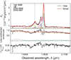 |
Fig. A.1. Fit fit obtained for the Hβ line if forcing the broadest component to fall at the same central velocity offset as the broadest component of Hα. |
All Tables
All Figures
|
Fig. 1. Spectral line profile of the Paβ line. Top panel: Observed Paβ line profile (black) from MIRI MRS channel 1, extracted within a 3-kpc radius. The red line corresponds to our best-fit model (red). The two individual Gaussian components are displayed on the bottom as green and magenta dashed lines (offset from zero by an arbitrary amount). We mask a noise spike (shown in grey) shortwards of the line. Middle panel: Continuum after multi-Gaussian line subtraction. Bottom panel: χ statistic corresponding to the residuals between the model and the observed spectral profile, divided by the rms error in the continuum. |
| In the text | |
|
Fig. 2. Same as Fig. 1, but for the Hα line covered by our NIRSpec observations. The Hα kinematic components are shown as dashed lines, while the (weak) dotted Gaussians correspond to [N II] and [S II]. |
| In the text | |
|
Fig. 3. Same as Fig. 1, but for the Hβ line covered by our NIRSpec observations. The dashed blue line in the middle panel shows the recovered contribution by the Fe II complex to the continuum, and the orange line is a linear fit to the residual continuum. The [O III] and He II lines are also covered, but not used in our analysis. |
| In the text | |
|
Fig. 4. Same as Fig. 1, but for the Mg II line covered by existing GNIRS observations. The dashed blue line in the middle panel shows the recovered contribution by the Fe II complex to the continuum. |
| In the text | |
|
Fig. 5. SED fit obtained for J1652 with the CIGALE code. The observed photometry is displayed by violet circles, and model fluxes are shown as red dots, while the black curve corresponds to the model spectrum. The different components included in the fit are: dust emission (red), AGN template (orange), nebular emission lines (green), and the host galaxy contribution (shown in blue and yellow, with and without dust attenuation, respectively). |
| In the text | |
|
Fig. 6. Comparison of line profiles. Left panel: Superposition of the Paβ (red) and Hα (black) line profiles in velocity space. The fluxes are in arbitrary units. There is a close match in the total line profiles, with the peaks (set by the narrow component) occurring at similar velocities assuming a redshift of z = 2.94. We omit the Hβ and Mg II profiles from this panel since they are strongly blended, but they can be seen in Figs. 3 and 4. The features shortwards of ∼ − 5000 km/s in the Paβ profile are masked in the fitting. Right panel: Superposition of the total line profiles of Paβ (red), Hα (black), Hβ (grey) and Mg II (blue) as recovered by our multi-Gaussian line fitting procedure (arbitrary flux units). |
| In the text | |
|
Fig. 7. Spread in virial BH mass estimates for J1652 recovered from the kinematics of different broad lines (Paβ: red symbols, Hα: black symbols, Hβ: grey symbols, Mg II: blue symbols) under varying assumptions, as specified by the labels on the y-axis. In the left panel, we rescaled all virial BH masses to a common virial factor f = 1, while in the right panel the original f values from the calibrations are applied (f = 4.31 for Paβ, f = 0.75 for the Balmer lines and f = 1 for Mg II). For each line, we show the mass recovered by using the total line profile (circles) versus the broadest component of our line fit only (diamonds), and observed fluxes (open circles) versus dust-corrected ones assuming AV = 0.89 mag (filled circles). The individual errorbars reflect the uncertainties quoted in the coefficients of the virial mass prescriptions (Eqs. (2), (3), and (4)), and we caution that they do not cover the range of BH masses obtained with our different assumptions for J1652. The vertical dashed line indicates the BH mass constraint by Perrotta et al. (2019) based on the galaxy-integrated Hβ emission in Gemini/GNIRS observations. The median log MBH among all of our estimates is indicated by the solid vertical line, with the shaded region corresponding to ±1 standard deviation. With four open rectangles, we highlight the treatment from the original calibrations in the right panel. |
| In the text | |
|
Fig. 8. Our range of recovered BH mass estimates for J1652 (grey bar) in the context of the low-redshift MBH–M⋆ relation for all broad-line AGNs (blue solid line; Reines & Volonteri 2015) and for ellipticals with suppressed star formation (blue solid line; Kormendy & Ho 2013). Depending on the choice of line (Paβ, Hα, Hβ, and Mg II) and underlying assumptions (assignment of kinematic components to the broad line region, virial factor, f, dust attenuation, etc.), and considering the uncertainties, one could argue that J1652 is overmassive or falls onto the MBH–M⋆ relation. The uncertainty on the stellar mass is derived from considering all SED models explored with a similar goodness of fit (χ2 within 5% of the best fit value). For context, we add a sample of massive high-redshift radio galaxies (green squares; De Breuck et al. 2010; Nesvadba et al. 2011), and unobscured X-ray AGNs at Cosmic Noon (purple circles; Suh et al. 2020). |
| In the text | |
|
Fig. A.1. Fit fit obtained for the Hβ line if forcing the broadest component to fall at the same central velocity offset as the broadest component of Hα. |
| In the text | |
Current usage metrics show cumulative count of Article Views (full-text article views including HTML views, PDF and ePub downloads, according to the available data) and Abstracts Views on Vision4Press platform.
Data correspond to usage on the plateform after 2015. The current usage metrics is available 48-96 hours after online publication and is updated daily on week days.
Initial download of the metrics may take a while.