| Issue |
A&A
Volume 684, April 2024
|
|
|---|---|---|
| Article Number | A52 | |
| Number of page(s) | 15 | |
| Section | Extragalactic astronomy | |
| DOI | https://doi.org/10.1051/0004-6361/202348138 | |
| Published online | 01 April 2024 | |
Broad-line region geometry from multiple emission lines in a single-epoch spectrum
1
Max Planck Institute for Extraterrestrial Physics (MPE), Giessenbachstr. 1, 85748 Garching, Germany
e-mail: This email address is being protected from spambots. You need JavaScript enabled to view it.
2
Department of Physics & Astronomy, University of British Columbia, 6224 Agricultural Road, Vancouver, BC V6T 1Z1, Canada
3
Kavli Institute for Astronomy and Astrophysics, Peking University, Beijing 100871, PR China
4
Department of Astrophysical & Planetary Sciences, JILA, University of Colorado, Duane Physics Bldg., 2000 Colorado Ave, Boulder, CO 80309, USA
5
Department of Physics, Technical University of Munich, James- Franck-Straße 1, 85748 Garching, Germany
6
Departments of Physics & Astronomy, Le Conte Hall, University of California, Berkeley, CA 94720, USA
7
Department of Physics and Astronomy, University of Southampton, Southampton, UK
8
School of Physics and Astronomy, Tel Aviv University, Tel Aviv 69978, Israel
Received:
3
October
2023
Accepted:
22
January
2024
Abstract
The broad-line region (BLR) of active galactic nuclei (AGNs) traces gas close to the central supermassive black hole (BH). Recent reverberation mapping (RM) and interferometric spectro-astrometry data have enabled detailed investigations of the BLR structure and dynamics as well as estimates of the BH mass. These exciting developments have motivated comparative investigations of BLR structures using different broad emission lines. In this work, we have developed a method to simultaneously model multiple broad lines of the BLR from a single-epoch spectrum. We applied this method to the five strongest broad emission lines (Hα, Hβ, Hγ, Paβ, and He Iλ5876) in the UV-to-near-IR spectrum of NGC 3783, a nearby Type I AGN that has been well studied by RM and interferometric observations. Fixing the BH mass to the published value, we fit these line profiles simultaneously to constrain the BLR structure. We find that the differences between line profiles can be explained almost entirely as being due to different radial distributions of the line emission. We find that using multiple lines in this way also enables one to measure some important physical parameters, such as the inclination angle and virial factor of the BLR. The ratios of the derived BLR time lags are consistent with the expectation of theoretical model calculations and RM measurements.
Key words: galaxies: active / galaxies: individual: NGC 3783 / quasars: emission lines / quasars: supermassive black holes / galaxies: Seyfert
© The Authors 2024
 Open Access article, published by EDP Sciences, under the terms of the Creative Commons Attribution License (https://creativecommons.org/licenses/by/4.0), which permits unrestricted use, distribution, and reproduction in any medium, provided the original work is properly cited.
This article is published in open access under the Subscribe to Open model.
Open access funding provided by Max Planck Society.
1. Introduction
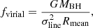
It is challenging to measure the mass of a supermassive black hole (BH) at the center of a galaxy because, ideally, one needs to resolve its sphere of influence (Kormendy & Ho 2013). This is true in the local Universe, where dynamical methods are preferred. At cosmic distances, one has to rely on scaling relations, except when the broad-line region (BLR) of an active galactic nucleus (AGN) is observable. The broad recombination lines with a typical full width at half maximum (FWHM) ≳1000 km s−1 (Khachikian & Weedman 1974) are emitted by the ionized gas surrounding the accreting BH (Peterson 1997). The BH mass can be derived with the virial method once the size of the BLR has been measured, MBH = fvirialRv2/G, where R is the BLR radius, v is a characteristic velocity of the BLR rotation, and fvirial is the virial factor that takes account of the geometry of the BLR. The structure and dynamics of the BLR strongly affect the virial factor and are critical to the BH mass measurement (Collin et al. 2006; Mejía-Restrepo et al. 2018).
The broad-line profile suggests that the BLR has a disk-like geometry (e.g., Wills & Browne 1986; Vestergaard et al. 2000; Kollatschny & Zetzl 2011; Shen & Ho 2014; Storchi-Bergmann et al. 2017). Its size is most often measured from the time lag between the AGN continuum and the broad emission line light curves by using the reverberation mapping (RM) technique (Blandford & McKee 1982; Peterson 2014). The characteristics of these time lags across different velocity channels have provided evidence of inflow and outflow motions in the BLR (e.g., Bentz et al. 2010a; Grier et al. 2013; Du et al. 2016). This has led to the development of comprehensive models that can constrain the BLR structure using high-quality RM data (Brewer et al. 2011; Pancoast et al. 2011, 2014a,b; Li et al. 2013). More recently, the BLR has been spatially resolved with spectro-astrometry, which is a powerful technique for measuring the BLR structure and BH mass (GRAVITY Collaboration 2018, 2020, 2021a, 2024), even out to the cosmic noon (Abuter et al. 2024). Attempts have been made to analyze spectro-astrometry and RM data jointly (hereafter, the SARM method) in order to measure the geometric distance of the BLR and better constrain the BLR structure and BH mass (Wang et al. 2020; GRAVITY Collaboration 2021b; Li et al. 2022).
The high-quality data needed for the detailed analyses described above are not widely available for large AGN samples, even with the ongoing large RM projects, such as SDSS-RM (Shen et al. 2015) and OzDES-RM (Malik et al. 2023). However, there is a wealth of AGN samples with good quality single-epoch spectra. To exploit these samples, Raimundo et al. (2019, 2020) modified the widely used BLR dynamical modeling code CARAMEL and used it to fit single-epoch line profiles. They were able to constrain some BLR model parameters, such as the inclination angle and disk thickness, and to estimate a BH mass by setting a prior on the BLR size based on the empirical size-luminosity relation (e.g., Bentz et al. 2013). We turn this idea around and focus on investigating the BLR structure and the virial factors derived from multiple broad lines, which are covered simultaneously in a spectrum across UV, optical and/or near-IR (NIR). By doing so, we can understand how the structure of the BLR changes between different lines within the same AGN. Previous RM observations found that higher ionization lines respond more promptly to continuum variations than lower ionization lines (e.g., Clavel et al. 1991; Gaskell 2009). The photoionization model, such as the “locally optimally emitting cloud” (LOC) model (Baldwin et al. 1995), can naturally produce such “radial ionization stratification”. Korista & Goad (2004) predicted decreasing time lags of Hα, Hβ, Hγ, He I, and He II using the LOC model, which were confirmed by the RM observation of nearby AGNs (Bentz et al. 2010b).
In this paper, we analyze the VLT/X-shooter (Vernet et al. 2011) spectrum of NGC 3783, which covers several strong, prominent broad emission lines of hydrogen and helium and for which the high spectral resolution enables a robust decomposition of the broad and narrow lines. These data were previously used in a study of BLR excitation and extinction in several AGN (Schnorr-Müller et al. 2016). For NGC 3783, Bentz et al. (2021a) reported the RM time lags of various lines, including Hβ and Hγ. Bentz et al. (2021b) performed dynamical modeling of Hβ and He II lines and derived a BLR size and BH mass consistent with the traditional method. GRAVITY Collaboration (2021a) reported the spectro-astrometry measurement of the broad Brγ line. This motivated a joint SARM analysis, which yielded consistent results (GRAVITY Collaboration 2021b). Here, we introduce the data and our method to decompose the broad-line profiles in Sect. 2. Then, we make a nonparametric characterization of them in Sect. 3. We discuss our modeling of the line profiles in Sect. 4, comparing our results with GRAVITY Collaboration (2021b) because the joint analysis provides the strongest constraint of the BLR model. We discuss the strengths and limitations of the current method in Sect. 5 and conclude in Sect. 6.
2. Data reprocessing of X-shooter spectra
2.1. Data reduction
The X-shooter data were acquired as part of the LLAMA project (Davies et al. 2015). A description of the observations and data reduction can be found in Schnorr-Müller et al. (2016) and Burtscher et al. (2021). We briefly summarize the key points as follows: NGC 3783 (11:39:01.7, −37:44:19.0) was observed with X-shooter at the Very Large Telescope in early 2014 using the IFU mode (program ID 092.B-0083). The spectral resolving power, R = λ/Δλ, is about 8400 (UVB), 13200 (VIS), and 8300 (NIR; Schnorr-Müller et al. 2016). The data were reduced with the ESO reflex pipeline (version 2.6.8) by using the Kepler GUI interface (Modigliani et al. 2010) and mostly the default configuration. The pipeline provides the data cubes of UVB, VIS, and NIR arms separately for each observation. Telluric and flux calibrator stars were also observed. Flux calibration was performed with a spectro-photometric standard from Moehler et al. (2014). From a comparison of the stars observed throughout the program, the spectrum was calibrated to an accuracy of about 2%. We extracted 1D spectra from each of the NGC 3783 data cubes using a rectangular slit with a width of 1.8″, and we applied minor scaling corrections to match the different spectral ranges.
We corrected the Galactic extinction based on AV = 0.332 (Schlafly & Finkbeiner 2011) and the Cardelli et al. (1989) extinction model, where we specified RV = 3.1 as the ratio of total to selective extinction, and we converted the spectrum to the rest frame, adopting a redshift of 0.00973 measured from the H I 21 cm line observations (Theureau et al. 1998). A final correction was made to the blue wing of the broad hydrogen lines in the UV arm due to absorption in the telluric star. We masked these narrow wavelength ranges (4286−4307 Å and 4800−4818 Å) when modeling the BLR profiles (Sect. 4). We also identified a few bad channels in the He Iλ5876 profile and some channels contaminated by absorption and emission lines of the sky in the Paβ profile. We masked these channels when we modeled the line profiles, noting that they are always much narrower than the broad-line profiles, so they will not affect the modeling. We present the optical and NIR parts of the spectrum that are relevant to this work in Fig. 1 together with the spectral decomposition that is discussed in Sect. 2.2.
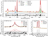 |
Fig. 1. X-shooter spectrum of NGC 3783 simultaneously covering UV, optical, and NIR ranges. In each panel, the spectrum is shown with the full model that enables decomposition of the broad-line profiles overplotted, and the residual is shown underneath. The emission line components are also plotted separately. The gray-shaded regions in the residuals represent wavelength ranges of bad channels and features due to the poor telluric correction, which are masked in the fitting. Panel a: UV/optical spectrum with the Hα, Hβ, and Hγ lines. Panel b: part of the NIR spectrum used in this study, with the Paβ line. Panel c: [S II] doublet used as the narrow line template. |
2.2. Spectral decomposition
We decomposed the broad-line components of Hα, Hβ, Hγ, and He Iλ5876 from the combined UVB and VIS spectra and the Paβ profile from the NIR spectrum. The final overall fit can be found in Fig. 1.
2.2.1. Narrow line template
The narrow line profiles of AGNs are usually more complex than a simple Gaussian profile, which argues for the use of a template based on isolated lines. The [S II] λλ6716,6731 and [O III] λλ4959,5007 lines are usually used for this purpose, and one can use multiple Gaussian components to generate a noiseless narrow line template (Ho et al. 1997). To generate the template, we fit each of the [S II] lines with three Gaussian profiles, tying their width and velocity shift from the laboratory wavelength between the pair but allowing the total scaling to vary. At the same time, we fit the local continuum with a third-order polynomial function. We found that neither more Gaussian components nor a higher-order polynomial function could improve the fitting. We adopted the [S II] doublet because the [O III] lines show stronger blue-shifted wind components. When trying a template based on [O III], we found it did not match the narrow line components of the H I lines well.
2.2.2. Decomposing the broad-line profiles
The continuum of an AGN optical spectrum consists of emission from the accretion disk, the host galaxy, and the pseudo-continuum of the Fe II lines (e.g., Barth et al. 2015). We adopted a power-law model for the AGN featureless continuum and found a host galaxy component based on Bruzual & Charlot (2003) stellar populations amounted to ≲10% of the continuum and was thus not needed. To fit the Fe II features, we incorporated the newly published high-quality template covering 4000−5600 Å (Park et al. 2022). We found the final normalized line profiles only change ≲0.05 if we adopt the Fe II template from Boroson & Green (1992), which has little effect on the BLR modeling results. We broadened and shifted the Fe II template as part of the fitting process. A wide wavelength range is useful for decomposing these components, so we opted to fit the entire optical spectrum over 4200−6800 Å and decompose the broad Hα, Hβ, Hγ, and He I profiles simultaneously (Fig. 1a). We describe fitting the more isolated Paβ line later in the text.
In the optical spectrum, the majority of narrow lines were fitted by the [S II] template with two free parameters, the amplitude and the velocity shift from the laboratory wavelength. We tied the velocity shifts of all the templates, so the fitting reflects a small deviation (≈ − 2 km s−1) from the redshift measured by the atomic H I gas. Because the UVB arm has a lower spectral resolution than the VIS arm, we broadened the narrow line template with a Gaussian kernel (σ ≈ 35 km s−1) for all lines at wavelengths shorter than 5600 Å. For the [O III] lines, which have a higher critical density and more contribution from blue-shifted components than [S II], we added additional Gaussian components: one for [O III] λ4363 and two (tied together and with a ratio of 2.98) for each line in the [O III] λλ4959,5007 doublet. The [N II] λ6550, 6585 doublets were fitted with the [S II] template with the amplitude ratio fixed to the theoretical value of 2.96. For completeness and to avoid influencing the continuum placement, we fitted several other narrow lines1 in the spectrum, although they do not directly affect the broad line decomposition.
For the broad lines, we found three Gaussian components are sufficient to fit the Hα, Hβ, Hγ, and He I profiles. We fit the broad He IIλ4686 as well, although it is too faint to provide a robust line profile for our dynamical modeling.
Lastly, we multiplied the entire optical spectrum model by a fifth-order polynomial function to account for large-scale variations caused by the instrumental and calibration effects (Cappellari 2017). This method can moderately improve the fitting of the continuum in the line wings at a level of ∼10−16 erg s−1 cm−2 Å−1.
In the NIR spectrum, we fitted the broad Paβ profile and continuum over a wavelength range of 12 400−13 300 Å. We included a power law for the continuum, the [S II] template (broadened to match the resolution of the NIR arm) for the narrow Paβ line, and three Gaussian components for the broad Paβ line. The velocity shift with respect to the theoretical wavelength of the narrow Paβ line was not tied to the optical narrow lines, but their velocity difference of ≲1.7 km s−1 is consistent with the systematic uncertainty of X-shooter wavelength calibration over different arms2. This high accuracy enabled us to tie the central wavelength offsets when we fit the broad-line profiles simultaneously (Sect. 4).
2.2.3. Resampling and uncertainties
While the high resolution of the X-shooter spectrum helps decompose the narrow- and broad-line profiles robustly, it is not necessary for the modeling, which is only constrained by the broad (≳1000 km s−1) and smooth features. Therefore, we resampled the decomposed line profiles to an effective resolving power of 2000, which is high enough to retain the characteristic features of the profiles while reducing the computational time. We also verified that our conclusions do not change with a slightly lower (R = 1000) or higher (R = 4000) resolution.
We first convolved the decomposed broad-line profiles with Gaussian kernels to the required resolution. Then, we used the Python tool SpectRes (Carnall 2017) to resample them while preserving the integrated flux and propagating the uncertainties. We chose the channel width of the re-sampled profiles to be ∼75 km s−1 so that the spectra are still Nyquist sampled.
To calculate the uncertainties of the line profiles, we summed two components in quadrature: (1) the uncertainty of the observed spectrum and the line profile decomposition, and (2) 5% of the line flux. To estimate the first component, we used a running root mean square (RMS) of the fitting residual of the original spectra, which includes the imperfectness of the fitting and other potential artifacts. The second component is important to avoid too much emphasis on the line center of the strongest lines (i.e., Hα and Hβ). Specifically, we adopted the following equation
 (1)
(1)
where RMSrun(res) is the running RMS over the spectrum residuals with a window size of 30, Norg/Ndwn is the ratio of the number of channels in the original spectrum over the downgraded spectrum3, and Fλ is the flux density.
As a final step, we normalized the line profiles and their uncertainties according to the peak of our multi-Gaussian model of the broad lines in Sect. 2.2.2. The resulting profiles are shown in Fig. 2. The centroid and width of the line peaks are consistent, while the width of the line wings varies for different lines. We note that the red wing of the broad Hγ overlaps with the [O III] λ4363 line, which we fit with the narrow line template plus a Gaussian component (Sect. 2.2.2). We opted to keep the [O III] λ4363 model simple to avoid biasing the Hγ profile. However, this resulted in a relatively large residual (0−2000 km s−1) and therefore uncertainty of the line profile, as shown in Fig. 2d. The Hγ line shows the strongest asymmetry due to the “shoulder” on the red wing, which is very difficult to model. We believe it can be at least partly explained in terms of the decomposition. In addition, the entire broad He I profile shows relatively large uncertainties because this line is very weak compared to the H I lines, and its uncertainties are dominated by the RMS term. Among the five broad lines studied in this work, He I is the most susceptible to any artifact of the spectrum.
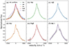 |
Fig. 2. Normalized broad emission line profiles of Hα, Hβ, Hγ, Paβ, and He I. These were extracted as described in Sect. 2.2. Panel a shows the profiles superimposed for an easier comparison, while panels b–f display the line profiles individually. The uncertainties are shown in gray. The masked data have been replaced by the multi-Gaussian model, as shown in Fig. 1 for clarity. |
3. Nonparametric properties of the broad-line profiles
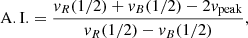
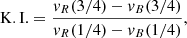
Because broad-line profiles cannot be described by a simple analytical function, we characterized them nonparametrically and later used these quantities (Table 1) to assess the validity of our model. The peak velocity, vpeak, is the deviation of the peak wavelength of the line from its expected wavelength after shifting to the rest frame, as described in Sect. 2.1. All of the broad lines peak near the systemic velocity. We calculated the full width at 25% (W25), 50% (FWHM; W50), and 75% (W75) maximum. We also calculated the asymmetry index (A.I.) and Kurtosis Index (K.I.) of each line profile as defined in Marziani et al. (1996),
 (2)
(2)
 (3)
(3)
Nonparametric properties of the broad-line profiles.
where vR(x) > 0 and vB(x) < 0 (x = 1/4, 1/2, or 3/4) are the velocity of line profiles at the corresponding fraction of the line peak on the red and blue wings, respectively. The values of A.I. indicate the direction and degree of asymmetry in the line profile shape. Differing slightly from the definition of Marziani et al. (1996), we calculated the A.I. at 50% (instead of 25%) of the peak flux because our line profiles become more symmetric toward the wings. A positive A.I. indicates that the line profiles are skewed toward the red side relative to the profile center. This suggests an excess of line emission or broader velocity distribution on the red side compared to the blue side. K.I., on the other hand, is essentially W75/W25. A Gaussian profile has K.I. ≈0.46. A smaller K.I. indicates that the line profile has a broader wing than a Gaussian profile, and vice versa. We also calculated the second moment of the line profiles, σline, following the definition of the Eq. (3) of Dalla Bontà et al. (2020) for completeness because σline is widely used in RM works to derive the BH mass (Peterson et al. 2004; Wang et al. 2019). To determine the uncertainty for each reported value, we randomly perturbed each profile using the uncertainties from Sect. 2.2.3, remeasured these quantities 500 times, and calculated the standard deviation of the results.
We compare these parameters in Fig. 3. The H I lines show almost the same widths at 75% and 50% of the line peaks. The Hα line shows the lowest W25, while Hβ shows the highest W25 among the H I lines. The line wing of Hβ is significantly broader than the other H I lines (see also Fig. 2). Although the Hβ region is complicated, the line wing cannot be biased by the spectral decomposition. As shown in Fig. 1, the broad Hβ line is much stronger than the (pseudo-)continuum and far enough from the [O III] lines. The He I line shows a comparable line width to the H I lines at its peak (W75) but becomes much broader toward the wing (W50 and W25). The σline of all lines are similar and in between their W50 and W75, respectively. We do not plot the σline in Fig. 3 for clarity. All the lines show measurable and positive A.I., and although the Balmer lines show differing values, there are large uncertainties. The K.I. values are similar among the lines and are smaller than that expected for a single Gaussian profile, indicating that the profiles are peaky with broad wings.
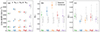 |
Fig. 3. Comparison of the nonparametric properties of the line profiles (denoted by different colors and with 1σ uncertainties). Panel a: line widths (circles, triangles, and squares represent W25, W50, and W75, respectively). Panel b: asymmetry index (A.I.). Panel c: kurtosis index (K.I.). In the panels, the gray lines correspond to equivalent measurements on the model line profiles for the separate (dotted) and combined (solid) fitting results. |
4. Modeling the broad-line profiles
In this section, we first introduce our BLR dynamical model, its limitations, and our inference strategy (Sect. 4.1). We then model the broad-line profiles in two steps: (1) We fit the line profiles separately and study the consistency of the model parameters (Sect. 4.2). (2) We fit the line profiles with almost all the BLR parameters tied and only allow the radial distribution of different line emissions to vary freely (Sect. 4.3).
4.1. Broad-line region dynamical model and the inference
The nature of the BLR is still an open question, and many models have been proposed to explain its various aspects (Peterson 2006; Czerny 2019, and references therein). One major class of models assumes that the BLR consists of many discrete clouds (e.g., Rees et al. 1989; Baldwin et al. 1995; Czerny & Hryniewicz 2011; Baskin & Laor 2018; Rosborough et al. 2023). The cloud model offers advantages in flexibly parameterizing the geometry, kinematics, and photoionization physics, enabling interpretation of observations, particularly recent high-quality RM and interferometric data (Korista & Goad 2004; Pancoast et al. 2011, 2014a; Li et al. 2013, 2018; Williams & Treu 2022; GRAVITY Collaboration 2018, 2020, 2021a). However, the physics of the cloud model may be oversimplified. For example, there is ongoing debate regarding the confinement of gas within high-density (≳109 cm−3) clouds (Mathews 1986; Rees 1987; Krolik 1988; Baskin et al. 2014; Proga et al. 2014; Proga & Waters 2015). Moreover, as discussed in detail by Netzer (2020), state-of-the-art cloud photoionization models tend to underproduce the luminosity of the Balmer lines (and other non-resonant H I lines) by a factor of two to five, likely due to the failure of escape probability formalism in photoionization codes such as CLOUDY (Ferland et al. 1998) for high densities and optical depths in the BLR. Radiation hydrodynamic simulations of the disk wind, coupled with radiative transfer calculations, have been deemed crucial to understanding the photoionization physics of the BLR (Waters et al. 2016; Matthews et al. 2016, 2020; Mangham et al. 2017). However, the high computational expense impedes the development of more comprehensive models for detailed data interpretation.
In this work, we employed our self-implemented BLR dynamical model to characterize the distribution and kinematics of the BLR line emission (or “emissivity”). The model parameterization was initially developed in Pancoast et al. (2014a). Our model has been utilized to fit the normalized line profile and differential phase signal, tracking the spatially resolved kinematics of recent interferometric observations of BLRs (GRAVITY Collaboration 2020, 2021a,b). Where our implementation differs from Pancoast et al. (2014a) is in using a Monte Carlo cloud model to depict the line emission at the moment of the observation, excluding variable continuum light curves and reverberation mapping physics. Thus, our modeling approach circumvents the challenges associated with the aforementioned photoionization physics of the BLR by modeling the line emission distribution instead of the physical clouds and photoionization physics. In making this statement, we emphasize that our use of the term “cloud” should be taken to mean “line emitting entity”. It does not refer to physical “gas clouds”, nor does it indicate a preference for the cloud model over the so-called disk-wind model (e.g., Chiang & Murray 1996; Matthews et al. 2016; Long et al. 2023). Here, we adapted the BLR model into a Python package, DyBEL, allowing the fitting of line profiles exclusively. The DyBEL package can be used to fit either a single line profile or multiple lines of an AGN simultaneously. As the detailed BLR model is presented in GRAVITY Collaboration (2020), we provide a brief introduction to the key parameters, which we summarize in Table 2.
Summary of the BLR model parameters, including a short explanation and prior range.
The model comprises a large number4 of non-interacting mass-less point particles orbiting the central BH with mass MBH and forming a disk-like structure. The radial distribution of the clouds follows a shifted Gamma function governed by three parameters: μ as the mean radius, F = Rmin/μ with Rmin as the minimum cloud radius, and β for the shape of the profile (Gaussian: 0 < β < 1; exponential: β = 1; and heavy-tailed: 1 < β < 2). The angular thickness of the disk is θo, and the vertical distribution of the clouds is governed by γ, with a higher value (γ > 1) corresponding to more clouds concentrating on the disk surface. The structure is viewed at an inclination angle i (with 0° corresponding to a face-on view). Each cloud is randomly assigned to be on a quasi-circular orbit with radial and tangential velocities (vr, vϕ) around (0,  ), or a quasi-radial orbit. The fraction on quasi-radial orbits is controlled by fellip (with fellip = 1 meaning all clouds are on such orbits). A binary parameter, fflow, governs the direction of the cloud radial motion. These clouds are inflowing if fflow < 0.5 or outflowing if fflow > 0.5. Their radial and tangential velocities are controlled by an angular parameter θe such that when θe = 0, the velocity vector is (
 , 0), and when θe = π/2, it is (0, vcirc). While Pancoast et al. (2014a) had additional parameters defining how the cloud velocities are dispersed around these points, we excluded them because they are generally unconstrained and do not influence our fitting (GRAVITY Collaboration 2020, 2021a,b). Finally, the weight of each cloud is controlled by −0.5 < κ < 0.5, reflecting the anisotropy of the cloud illumination. Clouds closer to the observer have higher weights if κ > 0, and vice versa. The ratio of clouds below and above the midplane is controlled by ξ, reflecting the “midplane obscuration” of the BLR. There are equal amounts of clouds between the midplane if ξ = 1, while there is no cloud below the midplane if ξ = 0. To fit the line profiles, we needed two nuisance parameters: the central wavelength (λc) and the peak flux (fpeak) of the line.
We used the above BLR model to describe the line emission distribution of the BLR without including any photoionization physics. We cannot predict the physical line luminosity with this model, so the line peak flux is a free parameter in the fitting, and we only modeled the normalized line profiles. This approach was adopted in the recent works GRAVITY Collaboration (2018, 2020, 2021a, 2024) when they modeled the line profile and differential phase data (equivalent to spatially resolved kinematic data). In contrast, the original application of this model to the RM data assumes the point particles to be “mirrors” reflecting the continuum emission, the limitations of which are nicely summarized by Raimundo et al. (2020, in their Sect. 2.2). Their arguments make it clear that photoionization physics are needed in the application of RM modeling. Indeed, there has been recent progress in addressing this problem (Williams & Treu 2022; Rosborough et al. 2023). Nevertheless, recent studies of NGC 3783 have shown that the modeling using GRAVITY and RM data is remarkably consistent (Bentz et al. 2021b; GRAVITY Collaboration 2021a,b), which supports the application of this simple model, at least for the particular case of NGC 3783. We discuss the caveats of applying this model to the single-epoch spectra, which is the main goal of this work, in Sect. 5.3.
We used the Python package dynesty (Speagle 2020) to fit the data with a nested sampling algorithm, which is more powerful than the typical Markov chain Monte Carlo method for complex models with many (e.g., more than 20) parameters and a potentially multimodal posterior distribution. By design, the nested sampling algorithm (Skilling 2004) can estimate the Bayes evidence, which enabled us to compare different models. We used the dynamic nested sampler (DynamicNestedSampler), which better estimates the likelihood function by re-sampling the posterior function a few more times after the “baseline run”. We used 1200 live points for the baseline run and added 500 points for each of the 10 re-samplings. We adopted the random walk algorithm (rwalk) to sample the prior space and used the multi-ellipse method (multi) to create the nest boundaries. We adopted the default values for all the remaining options of dynesty.
The metric we used to define the goodness of fit is the likelihood function,
 (4)
(4)
where the first summation over l is for different lines and the second summation over i is for different channels of a line profile; fl, i and σl, i are the line profile flux and uncertainty;  is the corresponding line model with the set of parameters Θl; and a temperature parameter T > 1 is included to effectively scale up the uncertainties of the data. The temperature makes the likelihood function less peaky, which facilitates proper estimation of the posterior distribution. We found that T = 16 is a suitable setting, and our fitting results are not sensitive to the specific choice of temperature (e.g., T = 8, 16, or 32).
We find it is important to bear in mind that when fitting only the line profiles, MBH and μ are fully degenerate. This is because the cloud velocities always scale with vcirc, which depends on MBH/r, and it means that one needs to fix the BH mass in order to investigate the BLR sizes. Therefore, we included physical prior information by fixing MBH = 107.4 M⊙ (GRAVITY Collaboration 2021b). The exact value of the MBH does not affect the derived BLR model parameters except for the BLR radius. We discuss this point in more detail in the following sections. Next, we set fflow, a binary flag, to decide the direction of the radial velocity of the clouds. While the previous modeling efforts all indicate radial inflow (Bentz et al. 2021b; GRAVITY Collaboration 2021a,b), by using line profiles alone, one cannot distinguish between inflow and outflow (either in the model or via the Bayes evidence) because there is no spatial information. We note that the specific choices of fflow do not affect our results. Therefore, we adopted an inflow model setting fflow < 0.5.
When fitting the line profiles simultaneously with DyBEL, we could choose to tie other parameters in addition to fixing the same BH mass. As our aim is to assess whether the difference in the line profiles can be attributed to radial differences in the line emission distribution for an otherwise fixed BLR geometry, we therefore left μ, F, and β free to vary for each line, while the remaining model parameters were tied. We also tied the central wavelength offsets for each line, allowing them to shift together by a small amount ϵ = λc/λair − 1, where λair is the nominal wavelength in air. We adopted a Gaussian prior centered at zero with a small standard deviation of 0.01 for ϵ because λc is expected to be close to λair. Similarly, we expected the normalized line peaks to be close to one, so we only adopted a single nuisance parameter, fpeak, in the fitting with a Gaussian prior centered at one with a standard deviation of 0.1. The priors of the remaining parameters were adopted from GRAVITY Collaboration (2020).
For comparison, we first fit each profile separately, then mainly discuss the results fitting all of the five lines simultaneously. In each case, we calculated several parameters derived from the fit, including the minimum radius, Rmin ≡ μF; the weighted mean radius, Rmean, of the BLR clouds; and the virial factor, fvirial (Eq. (5)).
4.2. Fitting the line profiles separately
In this section, we investigate what can be learned from fitting the five line profiles separately. We show a comparison of the data and the fitting results in Fig. 4. We generated 500 model line profiles with parameters randomly selected from the posterior samples of each line and plotted the median line profiles in panel a and the 68% confidence interval of each line in panels b–f. Qualitatively, the BLR model can fit the line profiles reasonably well. The median model profiles reflect the differences of the lines. The 68% confidence profiles largely enclose the data of all lines. The Hα and Hβ model profiles are more tightly constrained than the other three lines thanks to their smaller uncertainties. The most obvious mismatch comes from the Hγ line, due to the “shoulder” on the red wing, as noted in Sect. 2.2.3. The He I model profile shows some deviation from the data too, although always within the 1-σ uncertainty level.
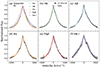 |
Fig. 4. Median and 68% confidence intervals of the model line profiles when the lines are fitted separately. The model profiles are overplotted in panel a, and the 68% confidence intervals of (b) Hα, (c) Hβ, (d) Hγ, (e) Paβ, and (f) He I are compared with the data (black). The masked data are not plotted, so gaps are visible in some profiles. |
The nonparametric parameters (line widths, A.I., and K.I.) for the model profiles are shown as vertical dotted lines in Fig. 3. The model line widths follow the corresponding lines remarkably well in all cases. The A.I. values show clear differences to the data, although largely within the uncertainties. In particular, the A.I. of Hγ is much higher than the model value. The K.I. values are consistent with the data, though the model posteriors tend to be higher.
There are 12 free parameters for each profile. The posterior distributions are displayed in Fig. 5. Following Raimundo et al. (2020), we considered a model parameter to be constrained if its 68% confidence range is less than half of its prior range. Consistent with these authors, we found the geometric parameters, i, θo, μ, and β, of most of the lines can be constrained, while the remaining parameters, fellip, κ, γ, ξ, and θe, mostly could not be constrained. The i and θo of Hα and Hβ agree well with the inclination derived by the SARM joint analysis (GRAVITY Collaboration 2021b), although these two parameters were less well constrained for Hγ, Paβ, and He I. In particular, the large asymmetry of Hγ led to a higher probability of a high inclination angle, so we observed tentative double-peaked posterior distributions for i and θo. In contrast, the distributions for Paβ and He I are broad and smooth, likely because the uncertainties of these two profiles are relatively large. The fits yielded generally small values for β (except Paβ), compared to the SARM result (β ≈ 1.95). This differs from the high value found in the SARM joint analysis but is consistent with the RM result for Hβ reported by Bentz et al. (2021a). Similarly, the minimum cloud radii (Rmin) for all lines except Paβ prefer smaller values than the SARM result. Nevertheless, the posteriors of the BLR sizes (Rmean) are largely consistent with the SARM results.
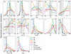 |
Fig. 5. Posterior probability distributions of the five lines fitted separately shown in colored histograms. For comparison, the dashed vertical line and the shaded region indicate the model inference best-fit results and 1-σ intervals from the SARM joint analysis (GRAVITY Collaboration 2021b). Panels a–i present the physical model parameters that are directly sampled in the fitting. The circles and crosses in these panels indicate whether these parameters are constrained by the data for each line profile (by comparing the width of their posterior distributions with their prior range). The remaining panels present parameters that are derived from the posterior samples. The y-axis tick labels are unimportant, so we removed them for clarity. Details are discussed in Sect. 4.2. |
4.3. Fitting the line profiles simultaneously
We performed a fit in which we tied all of the parameters of the BLR model for the five lines except those defining the radial distribution of the clouds, namely, μ, β, and F. With this approach, we could test whether the difference in the line profiles can be solely explained by the radial stratification of the BLR. There are 24 free parameters in the fit: nine tied between all the line profiles and three left separate for each of the five lines. We report the median and 68% confidence interval values of the combined fit posterior samples in Table 3. The model profiles and the 68% confidence intervals are shown in Fig. 6. Panel a of the figure shows that the model profiles of Hα, Hγ, and Paβ are very similar, while those of Hβ and He I are wider. This is similar to the results of the separate fitting. Because most of the model parameters were tied in this approach, we could conclude that the line profile differences can be explained by the radial distributions of the line emission. Moreover, the combined fit results showed tighter 68% confidence intervals than the separate fit. The improvement was most obvious in the Hγ, Paβ, and He I lines, whose uncertainties are relatively large. As a result, the deviation between the model and data of Hγ is more obvious.
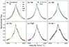 |
Fig. 6. Median and 68% confidence intervals of the model line profiles when the lines are fitted simultaneously with most of the parameters tied. The panels and symbols are the same as those of Fig. 4. |
Summary of the combined fitting results.
The nonparametric values for these model profiles are similar to those from the separate fits, while the uncertainties of the simultaneous fits are smaller than those of the separate fits. Again, they reproduce the line widths of the data well. The A.I. values are similar between the lines because the model parameters controlling asymmetry in the model (κ and ξ) were tied. We verified that if these are left free, the model yields different values of ξ to better fit the individual asymmetries of the lines. Meanwhile, the other parameters do not change substantially, and in neither case is the high asymmetry of Hγ reached. The K.I. values of the tied model profiles are more consistent with the data than those of the separate fits. We note that both model profiles yield σline consistent with the data profiles of all lines when fitting the data both separately and simultaneously.
Figure 7 shows that almost all of the tied model parameters are properly constrained and consistent with the SARM joint analysis. In particular, the distributions of β are similar to those from the separate fits except that Paβ now too prefers a lower value and thus matches the other lines. The lines also have similar Rmin ∼ 4 ld; hence, the line emission is concentrated in an inner ring and extends to large radii. In passing, we tested to further tie Rmin in the fit and found the results stay almost entirely the same with the tied Rmin ≈ 3.5 ld, confirming that the simultaneous fit favors the different lines sharing the same Rmin. GRAVITY Collaboration (2021b) tested fixing the Rmin = 4 ld in the SARM analysis and found a reasonable fitting result with β ≈ 1, which, interestingly, is close to our β. However, GRAVITY Collaboration (2021b) cautioned that additional restrictions bias their geometric distance measurement by about 30%.
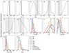 |
Fig. 7. Posterior probability distribution of the five lines fitted simultaneously with tied geometry parameters. The panels and symbols are similar to those of Fig. 5. For comparison, as before, the dashed vertical line and the shaded region indicate the model inference results from the joint SARM fit (GRAVITY Collaboration 2021b). |
The parameter that differs the most from the SARM result is γ, where a large value is preferred, indicating that the vertical distribution of line emission is more concentrated toward the surface of the BLR. However, there is a long tail toward low values in the posterior distribution of γ. The number of clouds in the mid-plane increases by less than 20% when γ decreases to 1.7 (the value derived in the SARM joint analysis), so the model does not change substantially. Nevertheless, the edge-concentrated structure with high γ may indicate that a biconical wind-like structure (e.g., Matthews et al. 2016; Waters et al. 2021) could fit the line profiles. The flexibility enabled by including such a capability in the model may allow it to better reproduce the asymmetric features in broad lines of NGC 3783.
5. Broad-line region geometry and virial factor from single-epoch line profiles
5.1. Broad-line region model parameters
In this section, we discuss the model parameters of the BLR that can be measured from single-epoch line profiles. For individual line profiles, we can constrain the inclination (i) and disk thickness (θo), a finding consistent with Raimundo et al. (2019, 2020). Because we fixed the BH mass, the radial distribution of the line emission can be constrained too. More interestingly, we find the BLR model can simultaneously fit multiple line profiles using the same geometry and kinematics. Almost all of the model parameters can be constrained, and only the radial distributions change for each line, indicating that the radial emissivity distributions are somewhat different, as expected (see the next paragraph). The H I lines tend to favor heavy-tailed distributions with β > 1, while the He I line is close to exponential (β ≈ 1). While it is beyond the scope of this work, we note that β ≳ 1 is close to a truncated power-law distribution that the photoionization model may produce (e.g., Netzer 2020).
Next, we compare the BLR radius (Rmean) of the combined fit of the five lines (Fig. 8a) with published measurements based on the Hβ and Brγ lines (Bentz et al. 2021a,b; GRAVITY Collaboration 2021a,b). We focused on the joint SARM analysis because it obtains the tightest constraints of the model parameters using the spectro-astrometry and RM data simultaneously and because we adopted its BH mass. The Rmean from the separate fitting shows relatively large uncertainties. The Rmean of Hβ, which happens to have the smallest uncertainty, is consistent with the Rmean derived by the SARM analysis. In contrast, Rmean derived from the combined fitting shows much smaller uncertainties, with the HβRmean consistent with the SARM result as well. The He IRmean is the smallest among the five lines. We note that the posterior distributions of Rmean are strongly correlated between different lines (Fig. A.1). While such a correlation increases the uncertainties of the mean radii (≳30%, Fig. 8a), as discussed in the next paragraph, it also means that the ratios of the mean radii have smaller uncertainties (≲10%).
 |
Fig. 8. Comparison of derived parameters. Values of (a) mean radius and (b) virial factor are shown for the separate (dotted lines) and combined (solid lines) fits. The three horizontal bars on each line correspond to the 16th, 50th, and 84th percentiles of the posterior distribution. The dashed lines and gray regions represent the results from the SARM joint analysis (GRAVITY Collaboration 2021b). |
As shown in Table 4, we measured the BLR mean radius ratios of Hα:Hβ:Hγ:Paβ:He I from the simultaneous fitting to be 1.47:1.0:1.22:1.36:0.72. They are largely consistent with the RM observation results reported by Bentz et al. (2010b). Our relative lags of the Hγ and He I lines are larger than the RM results. We also calculated the time lag ratios based on the radiation pressure confined (RPC) BLR model described by Netzer (2020). The theoretical model calculation explores a range of parameters that are in agreement with most RM measurements of various hydrogen and helium lines (e.g., Bentz et al. 2009, 2010b). The most important parameters of the RPC model are the radial dependence of the covering factor of the clouds, Rmin which is somewhat arbitrary, and the BLR outer radius, which is determined by graphite dust sublimation radius, gas metallicity, and turbulent velocity within individual clouds. The level of ionization and hence the line emissivity at all locations were obtained naturally from the assumption that the clouds’ column densities are large and that they are in total gas and radiation pressure equilibrium. The mean emissivity radius for each line was then computed from the model and then translated into time lags, which depend on the light curve of the driving continuum. All such models predict τHα > τHβ > τHγ > τHe I, and the range is illustrated in Table 4. Similar tendencies have also been predicted by the very different LOC model computed by Korista & Goad (2004).
Broad-line region size ratios.
We suspect our large Hγ radius is due to the error of the Hγ line profile. The Hγ line, the weakest among the three Balmer lines, is blended with [O III] λ4363 line (Fig. 1a). Therefore, the small but systematic residual of the decomposition may lead to a too large Hγ BLR size compared to its actual dimensions. The clear systematic deviations between the data and model in Fig. 6d support this point to some extent. This issue highlights the importance of high-quality line profiles in revealing robust BLR properties. Another effect that may influence the observed line emission distribution is the polar dust around the BLR (Hönig et al. 2013). Higher extinction in the center makes the BLR look more extended. Since extinction is larger at shorter wavelengths (Li 2007), this effect might enlarge the observed Hγ size more than Hα and Hβ. It is worth mentioning that Bentz et al. (2021a) reported a very small time lag of 3.7 ld for Hγ in NGC 3783, as small as that of He II. As discussed by the authors, the Hγ time lag was likely underestimated due to imperfect internal flux calibration using the [O III] λ5007 line flux. Observations of more targets would be useful to disentangle these effects on the measured BLR size across different lines.
We remind the readers that the models shown here do not include time-dependent variations of the ionizing source, and we caution that the flux- weighted radius (Rmean) may be different from the time lag, depending on the structure of the BLR and the ionization continuum light curve (Netzer & Maoz 1990). However, we expect the Rmean ratios from our simultaneous fitting to be close to the ratios of the time lags because the different lines are assumed to share the same BLR structure. To conclude, our analysis shows that different broad emission lines appear to share most of the geometry and kinematics of the BLR. The relative BLR sizes are largely consistent with the theoretical expectation of photoionization models. This suggests that one can combine spectro-astrometry and RM data of different lines in a joint analysis by tying most of the BLR model parameters of the two lines.
5.2. The virial factor
The virial factor encapsulates the geometry of the BLR by linking the BH mass to the measurable properties of BLR size and line width. In this paper, we define it as
 (5)
(5)
where σline is the second moment of the model line profile, Rmean is the mean radius of the BLR, and MBH is the fixed BH mass. A key property is that fvirial scales with MBH/r, where r indicates the BLR size. Although we fixed the BH mass of NGC 3783, the value of fvirial that we derived does not depend on MBH because the BLR radius is a free parameter in the fit. The reason, as explained in Sect. 4.1, is that MBH and μ (or Rmean) are fully degenerate in our model. These parameters scale together without changing the line profile. Therefore, we can expect to derive meaningful virial factors from the fit. To confirm this point, we fit the data with a fixed MBH = 106.4 M⊙ (10 times smaller) and got the same fvirial results.
As shown in Fig. 8b, the derived values from both the separate fit and the combined fit are consistent with that of the SARM joint analysis (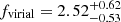 ). The combined fit shows smaller uncertainties than the separate fit. This is an encouraging result for investigating the BLR dynamics and measuring the BH mass. Our method could enable one to constrain the individual virial factor for each AGN by modeling the broad emission line(s) without the need for dynamical modeling of RM data (e.g., Villafaña et al. 2023). As a practical approach, one can fix the BH mass according to the single-epoch estimate (based on an averaged virial factor; McLure & Dunlop 2001; Ho & Kim 2015; Dalla Bontà et al. 2020) and model the broad-line profile(s) to derive the fvirial for individual AGNs. The fvirial can then be used to refine the BH mass estimate. As such, it could reduce the uncertainty in the BH mass that is otherwise introduced by adopting an average virial factor (Collin et al. 2006; Shen & Ho 2014). We caution that the derived virial factor may be biased by the oversimplified BLR model, the influence of which will be investigated with many more sources in the future.
5.3. Caveats
In this work, we have investigated the BLR structure by modeling the normalized single-epoch line profiles. We modeled the broad-line emission and the associated kinematics with a Monte Carlo model of points without a physical size. This model is intended to avoid consideration of the details of the photoionization physics and cannot predict the line strength physically according to the AGN luminosity. Without the data spatially resolving the BLR structure (e.g., GRAVITY differential phase), the model parameters may be degenerate when only fitted with the line profiles. Interestingly, for NGC 3783, we find the single-epoch line profiles, especially when fitted simultaneously, can provide most of the BLR model parameters in a manner consistent with the fitting that includes the size measurements. We caution, however, that more studies on different BLRs are needed to understand whether the conclusion holds widely.
To test whether our BLR model is quantitatively plausible with photoionization physics, we estimated the Hβ luminosity assuming the Case B recombination (Osterbrock & Ferland 2006) and the geometric covering factor based on our model fitting result. With θo ≈ 28.8° (Table 3), the geometric covering factor is sin θo ≈ 0.5. We adopted the ratio of the Hβ line and hydrogen recombination coefficients of 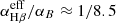 and the UV photon flux
 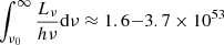 s−1 (ν0 = 13.6 eV), which is estimated with the measured λLλ(5100 Å) ≈ 4.1 × 1042 erg s−1 and the assumed AGN spectral energy distribution (SED) with low and intermediate Eddington ratios (Ferland et al. 2020; Jin et al. 2012) in order to enclose the range of typical Seyfert galaxy SEDs. We derive LHβ ≈ 0.4 − 0.9 × 1041 erg s−1. The measured Hβ luminosity5, ∼1.1 × 1041 erg s−1, is comparable to the estimated range, if not slightly higher, indicating that our BLR model is plausible in terms of line luminosity. While this estimate is admittedly oversimplified, it illustrates that the shape of the SED may easily influence the line luminosity by a factor of a few. It is worth noting that we assumed the maximum absorption of the UV photons with the model BLR geometry, and the Case B recombination does not consider the self-absorption of the Hβ photons. More detailed photoionization calculations with CLOUDY may only provide weaker line emission, which reflects the aforementioned problem in Sect. 4.1. Although this problem is beyond the scope of this work, our method provides a new approach to address it with single-epoch spectra.
6. Conclusions
We investigated the BLR structure of NGC 3783 using multiple broad lines in a high-resolution single-epoch spectrum obtained with VLT/X-shooter. We decomposed the five strongest broad lines (Hα, Hβ, Hγ, Paβ, and He Iλ5876), and modeled their profiles using the newly developed tool DyBEL, which allows one to tie parameters of the dynamical model between the lines. Since the BH mass and the BLR radius are fully degenerate, we opted to fix the BH mass to a value reported in the literature and focused on the BLR structure and emissivity that can be derived from the line profiles. Our main results are the following:
-
All lines analyzed here show broader wings than a Gaussian profile and are asymmetric (skewed to the red side). The He Iλ5876 profile is broader than the hydrogen profiles studied here.
-
We developed a fitting tool to model the line profiles with a dynamical BLR mode. Fitting multiple lines simultaneously by tying many of their parameters together yields a solution that is better constrained than when fitting them individually. In particular, it yields useful constraints on parameters such as inclination, BLR size, and the virial factor.
-
The difference in line profiles can be explained almost entirely in terms of differing radial distributions of the line emission. The derived relative BLR time lags are mostly consistent with the RM observation and with theoretical model calculations. Our results support that it is possible to combine spectro-astrometry and RM data in a joint analysis.
-
The virial factor we derived is nearly the same for the five lines and is independent of the adopted BH mass. We argue that by enabling one to constrain the virial factor for an individual AGN using a single-epoch spectrum, this method can reduce the uncertainty in BH masses derived from single-epoch spectra.
In the future, more comprehensive analyses will be useful to explore the potential of this method with more broad-line AGNs, different spectral resolutions and signal-to-noise ratios, and different BLR dynamical models.
We included [Fe V] λ4227, [O III] λ4363, He I λ4471, [Fe III] λ4658, [Ar IV] λ4711, [Ar IV] λ4740, [Fe VI] λ5146, [Fe VII] λ5159, [Fe VI] λ5176, [N I] λ5200, [Fe III] λ5270, [Fe VII] λ5276, [Ca V] λ5309, [Fe XIV] λ5303, [Fe VI] λ5335, [Fe VII] λ5721, [N II] λ5755, [Fe VII] λ6087, [O I] λ6300, [O I] λ6364, and [Fe X] λ6375. While we fit [O III] λ4363 with the narrow line template, we simply adopted a Gaussian function for the remaining narrow lines listed above.
We re-binned the spectrum profiles according to ratios of ∼2.26 and 3.32 for arms VIS and UVB/NIR, respectively.
We adopted 105 clouds in the fitting, which is large enough to produce smooth line profiles.
The measured λLλ(5100 Å) and LHβ are both from the X-shooter spectrum used in this work, so they may share the same systematic flux uncertainty, but it does not influence our comparison of Hβ luminosity.
Acknowledgments
L.K. thanks the financial support from the Mitacs Globalink Research Award. A.W.S.M. and L.K. acknowledge the support of the Natural Sciences and Engineering Research Council of Canada (NSERC) through grant reference number RGPIN-2021-03046. J.S. dedicates this paper in memory of his grandmother, G.X. (1930–2023). J.S. thanks Leonard Burtscher for sharing the X-shooter data.
References
- Abuter, R., Allouche, F., Amorim, A., et al. 2024, Nature, 627, 281 [NASA ADS] [CrossRef] [Google Scholar]
- Baldwin, J., Ferland, G., Korista, K., & Verner, D. 1995, ApJ, 455, L119 [NASA ADS] [Google Scholar]
- Barth, A. J., Bennert, V. N., Canalizo, G., et al. 2015, ApJS, 217, 26 [NASA ADS] [CrossRef] [Google Scholar]
- Baskin, A., & Laor, A. 2018, MNRAS, 474, 1970 [Google Scholar]
- Baskin, A., Laor, A., & Stern, J. 2014, MNRAS, 438, 604 [NASA ADS] [CrossRef] [Google Scholar]
- Bentz, M. C., Walsh, J. L., Barth, A. J., et al. 2009, ApJ, 705, 199 [NASA ADS] [CrossRef] [Google Scholar]
- Bentz, M. C., Horne, K., Barth, A. J., et al. 2010a, ApJ, 720, L46 [NASA ADS] [CrossRef] [Google Scholar]
- Bentz, M. C., Walsh, J. L., Barth, A. J., et al. 2010b, ApJ, 716, 993 [Google Scholar]
- Bentz, M. C., Denney, K. D., Grier, C. J., et al. 2013, ApJ, 767, 149 [Google Scholar]
- Bentz, M. C., Street, R., Onken, C. A., & Valluri, M. 2021a, ApJ, 906, 50 [Google Scholar]
- Bentz, M. C., Williams, P. R., Street, R., et al. 2021b, ApJ, 920, 112 [NASA ADS] [CrossRef] [Google Scholar]
- Blandford, R. D., & McKee, C. F. 1982, ApJ, 255, 419 [Google Scholar]
- Boroson, T. A., & Green, R. F. 1992, ApJS, 80, 109 [Google Scholar]
- Brewer, B. J., Treu, T., Pancoast, A., et al. 2011, ApJ, 733, L33 [NASA ADS] [CrossRef] [Google Scholar]
- Bruzual, G., & Charlot, S. 2003, MNRAS, 344, 1000 [NASA ADS] [CrossRef] [Google Scholar]
- Burtscher, L., Davies, R. I., Shimizu, T. T., et al. 2021, A&A, 654, A132 [NASA ADS] [CrossRef] [EDP Sciences] [Google Scholar]
- Cappellari, M. 2017, MNRAS, 466, 798 [Google Scholar]
- Cardelli, J. A., Clayton, G. C., & Mathis, J. S. 1989, ApJ, 345, 245 [Google Scholar]
- Carnall, A. C. 2017, arXiv e-prints [arXiv:1705.05165] [Google Scholar]
- Chiang, J., & Murray, N. 1996, ApJ, 466, 704 [NASA ADS] [CrossRef] [Google Scholar]
- Clavel, J., Reichert, G. A., Alloin, D., et al. 1991, ApJ, 366, 64 [NASA ADS] [CrossRef] [Google Scholar]
- Collin, S., Kawaguchi, T., Peterson, B. M., & Vestergaard, M. 2006, A&A, 456, 75 [NASA ADS] [CrossRef] [EDP Sciences] [Google Scholar]
- Czerny, B. 2019, Open Astron., 28, 200 [NASA ADS] [CrossRef] [Google Scholar]
- Czerny, B., & Hryniewicz, K. 2011, A&A, 525, L8 [NASA ADS] [CrossRef] [EDP Sciences] [Google Scholar]
- Dalla Bontà, E., Peterson, B. M., Bentz, M. C., et al. 2020, ApJ, 903, 112 [CrossRef] [Google Scholar]
- Davies, R. I., Burtscher, L., Rosario, D., et al. 2015, ApJ, 806, 127 [Google Scholar]
- Du, P., Lu, K.-X., Hu, C., et al. 2016, ApJ, 820, 27 [NASA ADS] [CrossRef] [Google Scholar]
- Ferland, G. J., Korista, K. T., Verner, D. A., et al. 1998, PASP, 110, 761 [Google Scholar]
- Ferland, G. J., Done, C., Jin, C., Landt, H., & Ward, M. J. 2020, MNRAS, 494, 5917 [Google Scholar]
- Gaskell, C. M. 2009, New Astron. Rev., 53, 140 [Google Scholar]
- GRAVITY Collaboration (Sturm, E., et al.) 2018, Nature, 563, 657 [Google Scholar]
- GRAVITY Collaboration (Amorim, A., et al.) 2020, A&A, 643, A154 [NASA ADS] [CrossRef] [EDP Sciences] [Google Scholar]
- GRAVITY Collaboration (Amorim, A., et al.) 2021a, A&A, 648, A117 [NASA ADS] [CrossRef] [EDP Sciences] [Google Scholar]
- GRAVITY Collaboration (Amorim, A., et al.) 2021b, A&A, 654, A85 [NASA ADS] [CrossRef] [EDP Sciences] [Google Scholar]
- GRAVITY Collaboration (Amorim, A., et al.) 2024, A&A, in press, https://doi.org/10.1051/0004-6361/202348167 [Google Scholar]
- Grier, C. J., Peterson, B. M., Horne, K., et al. 2013, ApJ, 764, 47 [NASA ADS] [CrossRef] [Google Scholar]
- Ho, L. C., & Kim, M. 2015, ApJ, 809, 123 [NASA ADS] [CrossRef] [Google Scholar]
- Ho, L. C., Filippenko, A. V., Sargent, W. L. W., & Peng, C. Y. 1997, ApJS, 112, 391 [NASA ADS] [CrossRef] [Google Scholar]
- Hönig, S. F., Kishimoto, M., Tristram, K. R. W., et al. 2013, ApJ, 771, 87 [Google Scholar]
- Jin, C., Ward, M., & Done, C. 2012, MNRAS, 425, 907 [NASA ADS] [CrossRef] [Google Scholar]
- Khachikian, E. Y., & Weedman, D. W. 1974, ApJ, 192, 581 [NASA ADS] [CrossRef] [Google Scholar]
- Kollatschny, W., & Zetzl, M. 2011, Nature, 470, 366 [NASA ADS] [CrossRef] [Google Scholar]
- Korista, K. T., & Goad, M. R. 2004, ApJ, 606, 749 [NASA ADS] [CrossRef] [Google Scholar]
- Kormendy, J., & Ho, L. C. 2013, ARA&A, 51, 511 [Google Scholar]
- Krolik, J. H. 1988, ApJ, 325, 148 [NASA ADS] [CrossRef] [Google Scholar]
- Li, A. 2007, in The Central Engine of Active Galactic Nuclei, eds. L. C. Ho, & J. W. Wang, ASP Conf. Ser., 373, 561 [NASA ADS] [Google Scholar]
- Li, Y.-R., Wang, J.-M., Ho, L. C., Du, P., & Bai, J.-M. 2013, ApJ, 779, 110 [NASA ADS] [CrossRef] [Google Scholar]
- Li, Y.-R., Songsheng, Y.-Y., Qiu, J., et al. 2018, ApJ, 869, 137 [CrossRef] [Google Scholar]
- Li, Y.-R., Wang, J.-M., Songsheng, Y.-Y., et al. 2022, ApJ, 927, 58 [NASA ADS] [CrossRef] [Google Scholar]
- Long, K., Dexter, J., Cao, Y., et al. 2023, ApJ, 953, 184 [NASA ADS] [CrossRef] [Google Scholar]
- Malik, U., Sharp, R., Penton, A., et al. 2023, MNRAS, 520, 2009 [NASA ADS] [CrossRef] [Google Scholar]
- Mangham, S. W., Knigge, C., Matthews, J. H., et al. 2017, MNRAS, 471, 4788 [CrossRef] [Google Scholar]
- Marziani, P., Sulentic, J. W., Dultzin-Hacyan, D., Calvani, M., & Moles, M. 1996, ApJS, 104, 37 [Google Scholar]
- Mathews, W. G. 1986, ApJ, 305, 187 [NASA ADS] [CrossRef] [Google Scholar]
- Matthews, J. H., Knigge, C., Long, K. S., et al. 2016, MNRAS, 458, 293 [NASA ADS] [CrossRef] [Google Scholar]
- Matthews, J. H., Knigge, C., Higginbottom, N., et al. 2020, MNRAS, 492, 5540 [NASA ADS] [CrossRef] [Google Scholar]
- McLure, R. J., & Dunlop, J. S. 2001, MNRAS, 327, 199 [NASA ADS] [CrossRef] [Google Scholar]
- Mejía-Restrepo, J. E., Lira, P., Netzer, H., Trakhtenbrot, B., & Capellupo, D. M. 2018, Nat. Astron., 2, 63 [CrossRef] [Google Scholar]
- Modigliani, A., Goldoni, P., Royer, F., et al. 2010, in Observatory Operations: Strategies, Processes, and Systems III, eds. D. R. Silva, A. B. Peck, & B. T. Soifer, SPIE Conf. Ser., 7737, 773728 [NASA ADS] [CrossRef] [Google Scholar]
- Moehler, S., Modigliani, A., Freudling, W., et al. 2014, A&A, 568, A9 [NASA ADS] [CrossRef] [EDP Sciences] [Google Scholar]
- Netzer, H. 2020, MNRAS, 494, 1611 [NASA ADS] [CrossRef] [Google Scholar]
- Netzer, H., & Maoz, D. 1990, ApJ, 365, L5 [NASA ADS] [CrossRef] [Google Scholar]
- Osterbrock, D. E., & Ferland, G. J. 2006, Astrophysics of Gaseous Nebulae and Active Galactic Nuclei (Sausalito: University Science Books) [Google Scholar]
- Pancoast, A., Brewer, B. J., & Treu, T. 2011, ApJ, 730, 139 [NASA ADS] [CrossRef] [Google Scholar]
- Pancoast, A., Brewer, B. J., & Treu, T. 2014a, MNRAS, 445, 3055 [Google Scholar]
- Pancoast, A., Brewer, B. J., Treu, T., et al. 2014b, MNRAS, 445, 3073 [Google Scholar]
- Park, D., Barth, A. J., Ho, L. C., & Laor, A. 2022, ApJS, 258, 38 [NASA ADS] [CrossRef] [Google Scholar]
- Peterson, B. M. 1997, An Introduction to Active Galactic Nuclei (Cambridge: Cambridge University Press) [Google Scholar]
- Peterson, B. M. 2006, in Physics of Active Galactic Nuclei at all Scales, ed. D. Alloin, (Berlin: Springer Verlag), Lect. Notes Phys., 693, 77 [NASA ADS] [CrossRef] [Google Scholar]
- Peterson, B. M. 2014, Space Sci. Rev., 183, 253 [Google Scholar]
- Peterson, B. M., Ferrarese, L., Gilbert, K. M., et al. 2004, ApJ, 613, 682 [Google Scholar]
- Proga, D., & Waters, T. 2015, ApJ, 804, 137 [NASA ADS] [CrossRef] [Google Scholar]
- Proga, D., Jiang, Y.-F., Davis, S. W., Stone, J. M., & Smith, D. 2014, ApJ, 780, 51 [Google Scholar]
- Raimundo, S. I., Pancoast, A., Vestergaard, M., Goad, M. R., & Barth, A. J. 2019, MNRAS, 489, 1899 [Google Scholar]
- Raimundo, S. I., Vestergaard, M., Goad, M. R., et al. 2020, MNRAS, 493, 1227 [Google Scholar]
- Rees, M. J. 1987, MNRAS, 228, 47P [NASA ADS] [CrossRef] [Google Scholar]
- Rees, M. J., Netzer, H., & Ferland, G. J. 1989, ApJ, 347, 640 [Google Scholar]
- Rosborough, S., Robinson, A., Almeyda, T., & Noll, M. 2023, arXiv e-prints [arXiv:2311.03590] [Google Scholar]
- Schlafly, E. F., & Finkbeiner, D. P. 2011, ApJ, 737, 103 [Google Scholar]
- Schnorr-Müller, A., Davies, R. I., Korista, K. T., et al. 2016, MNRAS, 462, 3570 [Google Scholar]
- Shen, Y., & Ho, L. C. 2014, Nature, 513, 210 [NASA ADS] [CrossRef] [Google Scholar]
- Shen, Y., Brandt, W. N., Dawson, K. S., et al. 2015, ApJS, 216, 4 [Google Scholar]
- Skilling, J. 2004, in Bayesian Inference and Maximum Entropy Methods in Science and Engineering: 24th International Workshop on Bayesian Inference and Maximum Entropy Methods in Science and Engineering, eds. R. Fischer, R. Preuss, & U. V. Toussaint, AIP Conf. Ser., 735, 395 [NASA ADS] [CrossRef] [Google Scholar]
- Speagle, J. S. 2020, MNRAS, 493, 3132 [Google Scholar]
- Storchi-Bergmann, T., Schimoia, J. S., Peterson, B. M., et al. 2017, ApJ, 835, 236 [Google Scholar]
- Theureau, G., Bottinelli, L., Coudreau-Durand, N., et al. 1998, A&AS, 130, 333 [NASA ADS] [CrossRef] [EDP Sciences] [Google Scholar]
- Vernet, J., Dekker, H., D’Odorico, S., et al. 2011, A&A, 536, A105 [NASA ADS] [CrossRef] [EDP Sciences] [Google Scholar]
- Vestergaard, M., Wilkes, B. J., & Barthel, P. D. 2000, ApJ, 538, L103 [CrossRef] [Google Scholar]
- Villafaña, L., Williams, P. R., Treu, T., et al. 2023, ApJ, 948, 95 [CrossRef] [Google Scholar]
- Wang, S., Shen, Y., Jiang, L., et al. 2019, ApJ, 882, 4 [CrossRef] [Google Scholar]
- Wang, J.-M., Songsheng, Y.-Y., Li, Y.-R., Du, P., & Zhang, Z.-X. 2020, Nat. Astron., 4, 517 [NASA ADS] [CrossRef] [Google Scholar]
- Waters, T., Kashi, A., Proga, D., et al. 2016, ApJ, 827, 53 [NASA ADS] [CrossRef] [Google Scholar]
- Waters, T., Proga, D., & Dannen, R. 2021, ApJ, 914, 62 [NASA ADS] [CrossRef] [Google Scholar]
- Williams, P. R., & Treu, T. 2022, ApJ, 935, 128 [NASA ADS] [CrossRef] [Google Scholar]
- Wills, B. J., & Browne, I. W. A. 1986, ApJ, 302, 56 [NASA ADS] [CrossRef] [Google Scholar]
Appendix A: Simultaneous fitting results with all parameters tied
The corner plot of the simultaneous fitting is shown in Figure A.1. The separate fittings show similar but less constrained results. We opted not to show all of the corner plots of the separate fitting for simplicity because all of the useful information has been shown in Figure 5.
 |
Fig. A.1. Corner plot of the simultaneous fitting. The first nine parameters are tied in the fitting, while the remaining parameters are fitted for individual lines. |
All Tables
Summary of the BLR model parameters, including a short explanation and prior range.
All Figures
|
Fig. 1. X-shooter spectrum of NGC 3783 simultaneously covering UV, optical, and NIR ranges. In each panel, the spectrum is shown with the full model that enables decomposition of the broad-line profiles overplotted, and the residual is shown underneath. The emission line components are also plotted separately. The gray-shaded regions in the residuals represent wavelength ranges of bad channels and features due to the poor telluric correction, which are masked in the fitting. Panel a: UV/optical spectrum with the Hα, Hβ, and Hγ lines. Panel b: part of the NIR spectrum used in this study, with the Paβ line. Panel c: [S II] doublet used as the narrow line template. |
| In the text | |
|
Fig. 2. Normalized broad emission line profiles of Hα, Hβ, Hγ, Paβ, and He I. These were extracted as described in Sect. 2.2. Panel a shows the profiles superimposed for an easier comparison, while panels b–f display the line profiles individually. The uncertainties are shown in gray. The masked data have been replaced by the multi-Gaussian model, as shown in Fig. 1 for clarity. |
| In the text | |
|
Fig. 3. Comparison of the nonparametric properties of the line profiles (denoted by different colors and with 1σ uncertainties). Panel a: line widths (circles, triangles, and squares represent W25, W50, and W75, respectively). Panel b: asymmetry index (A.I.). Panel c: kurtosis index (K.I.). In the panels, the gray lines correspond to equivalent measurements on the model line profiles for the separate (dotted) and combined (solid) fitting results. |
| In the text | |
|
Fig. 4. Median and 68% confidence intervals of the model line profiles when the lines are fitted separately. The model profiles are overplotted in panel a, and the 68% confidence intervals of (b) Hα, (c) Hβ, (d) Hγ, (e) Paβ, and (f) He I are compared with the data (black). The masked data are not plotted, so gaps are visible in some profiles. |
| In the text | |
|
Fig. 5. Posterior probability distributions of the five lines fitted separately shown in colored histograms. For comparison, the dashed vertical line and the shaded region indicate the model inference best-fit results and 1-σ intervals from the SARM joint analysis (GRAVITY Collaboration 2021b). Panels a–i present the physical model parameters that are directly sampled in the fitting. The circles and crosses in these panels indicate whether these parameters are constrained by the data for each line profile (by comparing the width of their posterior distributions with their prior range). The remaining panels present parameters that are derived from the posterior samples. The y-axis tick labels are unimportant, so we removed them for clarity. Details are discussed in Sect. 4.2. |
| In the text | |
|
Fig. 6. Median and 68% confidence intervals of the model line profiles when the lines are fitted simultaneously with most of the parameters tied. The panels and symbols are the same as those of Fig. 4. |
| In the text | |
|
Fig. 7. Posterior probability distribution of the five lines fitted simultaneously with tied geometry parameters. The panels and symbols are similar to those of Fig. 5. For comparison, as before, the dashed vertical line and the shaded region indicate the model inference results from the joint SARM fit (GRAVITY Collaboration 2021b). |
| In the text | |
|
Fig. 8. Comparison of derived parameters. Values of (a) mean radius and (b) virial factor are shown for the separate (dotted lines) and combined (solid lines) fits. The three horizontal bars on each line correspond to the 16th, 50th, and 84th percentiles of the posterior distribution. The dashed lines and gray regions represent the results from the SARM joint analysis (GRAVITY Collaboration 2021b). |
| In the text | |
|
Fig. A.1. Corner plot of the simultaneous fitting. The first nine parameters are tied in the fitting, while the remaining parameters are fitted for individual lines. |
| In the text | |
Current usage metrics show cumulative count of Article Views (full-text article views including HTML views, PDF and ePub downloads, according to the available data) and Abstracts Views on Vision4Press platform.
Data correspond to usage on the plateform after 2015. The current usage metrics is available 48-96 hours after online publication and is updated daily on week days.
Initial download of the metrics may take a while.