| Issue |
A&A
Volume 654, October 2021
|
|
|---|---|---|
| Article Number | A85 | |
| Number of page(s) | 14 | |
| Section | Extragalactic astronomy | |
| DOI | https://doi.org/10.1051/0004-6361/202141426 | |
| Published online | 15 October 2021 | |
A geometric distance to the supermassive black Hole of NGC 3783
1
Max Planck Institute for Extraterrestrial Physics (MPE), Giessenbachstr.1, 85748 Garching, Germany
e-mail: This email address is being protected from spambots. You need JavaScript enabled to view it.
2
LESIA, Observatoire de Paris, Université PSL, CNRS, Sorbonne Université, Univ. Paris Diderot, Sorbonne Paris Cité, 5 place Jules Janssen, 92195 Meudon, France
3
I. Institute of Physics, University of Cologne, Zülpicher Straße 77, 50937 Cologne, Germany
4
Departments of Physics and Astronomy, Le Conte Hall, University of California, Berkeley, CA 94720, USA
5
Department of Physics and Astronomy, University of Southampton, Southampton, UK
6
Department of Physics, Kyoto Sangyo University, Kita-ku, Japan
7
Université Côte d’Azur, Observatoire de la Côte d’Azur, CNRS, Laboratoire Lagrange, Nice, France
8
School of Physics and Astronomy, Tel Aviv University, Tel Aviv 69978, Israel
9
Univ. Grenoble Alpes, CNRS, IPAG, 38000 Grenoble, France
10
Center for Computational Astrophysics, Flatiron Institute, 162 5th Ave., New York, NY 10010, USA
11
European Southern Observatory, Casilla, 19001 Santiago 19, Chile
12
European Southern Observatory, Karl-Schwarzschild-Str. 2, 85748 Garching, Germany
13
Sterrewacht Leiden, Leiden University, Postbus 9513, 2300 RA Leiden, The Netherlands
14
Max Planck Institute for Radio Astronomy, Auf dem Hügel 69, 53121 Bonn, Germany
15
Universidade de Lisboa – Faculdade de Ciências, Campo Grande, 1749-016 Lisboa, Portugal
16
Faculdade de Engenharia, Universidade do Porto, rua Dr. Roberto Frias, 4200-465 Porto, Portugal
17
CENTRA – Centro de Astrofísica e Gravitação, IST, Universidade de Lisboa, 1049-001 Lisboa, Portugal
18
Max Planck Institute for Astronomy, Königstuhl 17, 69117 Heidelberg, Germany
19
Instituto de Astrofísica de Canarias (IAC), 38200 La Laguna, Tenerife, Spain
20
Department of Astrophysical & Planetary Sciences, JILA, University of Colorado, Duane Physics Bldg., 2000 Colorado Ave, Boulder, CO 80309, USA
21
Research School of Astronomy and Astrophysics, Australian National University, Canberra, ACT 2611, Australia
22
Department of Physics, Technical University Munich, James-Franck-Straße 1, 85748 Garching, Germany
23
Department of Physics and Astronomy, Georgia State University, Atlanta, GA 30303, USA
24
LCOGT, 6740 Cortona Drive, Suite 102, Goleta, CA 93117, USA
Received:
29
May
2021
Accepted:
24
July
2021
Abstract
The angular size of the broad line region (BLR) of the nearby active galactic nucleus NGC 3783 has been spatially resolved by recent observations with VLTI/GRAVITY. A reverberation mapping (RM) campaign has also recently obtained high quality light curves and measured the linear size of the BLR in a way that is complementary to the GRAVITY measurement. The size and kinematics of the BLR can be better constrained by a joint analysis that combines both GRAVITY and RM data. This, in turn, allows us to obtain the mass of the supermassive black hole in NGC 3783 with an accuracy that is about a factor of two better than that inferred from GRAVITY data alone. We derive MBH = 2.54−0.72+0.90 × 10⁷ M⊙. Finally, and perhaps most notably, we are able to measure a geometric distance to NGC 3783 of 39.9−11.9+14.5 Mpc. We are able to test the robustness of the BLR-based geometric distance with measurements based on the Tully–Fisher relation and other indirect methods. We find the geometric distance is consistent with other methods within their scatter. We explore the potential of BLR-based geometric distances to directly constrain the Hubble constant, H0, and identify differential phase uncertainties as the current dominant limitation to the H0 measurement precision for individual sources.
Key words: galaxies: active / galaxies: Seyfert / quasars: individual: NGC 3783 / distance scale / galaxies: nuclei
GRAVITY is developed in a collaboration by the Max Planck Institute for extraterrestrial Physics, LESIA of Observatoire de Paris/Université PSL/CNRS/Sorbonne Université/Université de Paris and IPAG of Université Grenoble Alpes/CNRS, the Max Planck Institute for Astronomy, the University of Cologne, the CENTRA – Centro de Astrofisica e Gravitaçã, and the European Southern Observatory.
© GRAVITY Collaboration 2021
 Open Access article, published by EDP Sciences, under the terms of the Creative Commons Attribution License (https://creativecommons.org/licenses/by/4.0), which permits unrestricted use, distribution, and reproduction in any medium, provided the original work is properly cited.
Open Access funding provided by Max Planck Society.
1. Introduction
Trigonometry is the basis of distance measurements. The parallax method uses the motion of the Earth around the Sun to measure the angular displacement of a nearby star (Bessel 1838). From the HIPPARCOS satellite of the European Space Agency (ESA; ESA 1997) to the recent Gaia mission (Gaia Collaboration 2016), the parallaxes of more than 1 billion stars in the Milky Way have now been measured (Gaia Collaboration 2018). The geometric method can also be applied to any object, as long as both its physical size (R) and angular size (Θ) are measurable, as D = R/Θ. For a distant extragalactic target, the measured geometric distance is the angular diameter distance (DA), including cosmological expansion. In contrast to “standard candles,” such as pulsating stars (e.g., Bhardwaj 2020) and Type Ia supernovae (SNe Ia; e.g., Phillips 1993; Riess et al. 1996), which measure the luminosity distance (DL), the geometric method does not rely on the calibration based on the so-called distance ladder (e.g., Riess et al. 2009; 2021).
However, objects to which the geometric method can be applied are usually rare as it is difficult to measure both R and Θ for the same target. The distance to the supermassive black hole (BH) at the center of the Milky Way is measured to a < 0.5% uncertainty level, based on the 27-year astrometric and spectroscopic monitoring of the 16-year orbital motion of the star S2 (Gravity Collaboration 2019). For detached eclipsing binary stars, the linear size of each component can be measured from photometric and spectroscopic monitoring, while the angular size of each star can be derived from its empirical relation with the color of the star (Lacy 1977). This method has been used to measure the distance to the Large Magellanic Cloud with high accuracy (Pietrzyński et al. 2019). By monitoring the Keplerian motion of water maser-emitting gas with very long baseline interferometry (VLBI) observations, one can measure the geometric distance to nearby Type-2 Seyfert galaxies that host an observable megamaser disk (Herrnstein et al. 1999; Braatz et al. 2010). Baryonic acoustic oscillations can also provide DA using the clustering of galaxies at a certain redshift range (e.g., Eisenstein et al. 2005; Anderson et al. 2014). The broad line region (BLR) of active galactic nuclei (AGNs) has also been proposed as a probe of geometric distance (Elvis & Karovska 2002). The linear size of the BLR can be measured by the reverberation mapping (RM) technique (Peterson 2014), while the angular size of the BLR can be measured by near-infrared (NIR) interferometry (Petrov et al. 2001; Woillez et al. 2004). Unlike detached eclipsing binaries and megamaser systems, which are difficult to discover, AGNs are luminous sources that are commonly found locally as well as out to high redshifts, even at z > 6. A similar approach has been applied to NGC 4151 by resolving the hot dust continuum emission instead of the BLR (Hönig et al. 2014).
Recently, GRAVITY, the second generation Very Large Telescope Interferometer (VLTI) instrument, spatially resolved the BLR of 3C 273 for the first time using the spectroastrometry (SA) technique (Bailey et al. 1998). GRAVITY combines all four of the 8 m Unit Telescope (UT) beams to yield six simultaneous baselines (Gravity Collaboration 2017). Gravity Collaboration (2018) reported the mean radius of the BLR as 46 ± 10 μas and a BH mass of (2.6 ± 1.1) × 108 M⊙, which is fully consistent with that measured by Zhang et al. (2019) using 10 year RM data. Wang et al. (2020) conducted the first joint analysis (hereafter, SARM, as the combination of SA and RM) and derived an angular diameter distance for 3C 273 of  Mpc, corresponding to a Hubble constant
  .
.
The Hubble constant has been measured to an accuracy of a few percent in the low-z Universe with various methods. Using the distance ladder, the SH0ES (supernovae H0 for the equation of state) project recently derived H0 = 73.5 ± 1.4 km s−1 Mpc−1 (Reid et al. 2019). This value is consistent with other measurements independent of the distance ladder, such as megamaser observations (e.g., Pesce et al. 2020) and observations of gravitationally lensed quasars (e.g., Wong et al. 2020) based on the so-called time-delay distance. In comparison, H0 inferred from conditions in the early Universe tends to be substantially smaller than the low-z values (4–6σ significance level, Riess 2020; however, see Freedman et al. 2019). For instance, Planck Collaboration VI (2020) derive 67.4 ± 0.5 km s−1 Mpc−1 based on cosmic microwave background observations. The high luminosity and remarkably uniform spectral properties of AGNs have motivated many attempts to use them as standard candles (Baldwin 1977; Collier et al. 1999; Elvis & Karovska 2002; Watson et al. 2011; Wang et al. 2013; Hönig 2014; La Franca et al. 2014; Risaliti & Lusso 2015). In particular, the good correlation between the BLR radius and continuum luminosity (e.g., Kaspi et al. 2000; Bentz et al. 2013) makes it promising to probe the DL based on the RM measurements (e.g., Watson et al. 2011; Wang et al. 2013). However, recent studies reveal significant deviations from the R–L relation, primarily driven by the increase in the Eddington ratio (Du et al. 2016, 2018; Du & Wang 2019; Martínez-Aldama et al. 2019; Dalla Bontà et al. 2020; however, see Grier et al. 2017; Fonseca Alvarez et al. 2020). It is therefore of great importance to explore the power of the SARM method, namely to study the BLR structure in detail and to measure the BLR-based geometric distance with the goal to independently test the H0 tension in the future.
With z ≈ 0.009730 (Theureau et al. 1998) and a much shorter time lag than that of 3C 273, NGC 3783 provides the best opportunity to compare the geometric distance derived with SARM to other independent measurements. A new RM campaign of NGC 3783 was reported by Bentz et al. (2021) with a time lag of about 10 days, consistent with previous measurements (Onken & Peterson 2002). Gravity Collaboration (2021, hereafter, GC21) reported a BLR mean angular radius of about 70 μas, and the RM-measured time lag can be reproduced with the measured continuum light curve and the best-fit BLR model inferred only from GRAVITY data at an assumed DA = 38.5 Mpc. In this paper, we construct a Bayesian model to fit the GRAVITY and RM data simultaneously (Sect. 3). The inferred BLR model is entirely consistent with the results of GC21 (Sect. 4). We find that the inferred DA of NGC 3783 is fully consistent with distances measured using the Tully–Fisher relation and other indirect methods (Sect. 5). The application of the SARM method to H0 is discussed in Sect. 5.4, together with improvements that may come with the ongoing upgrade of the GRAVITY instrument. This work adopts the following fiducial parameters for a ΛCDM cosmology: Ωm = 0.3, ΩΛ = 0.7, and H0 = 70 km s−1 Mpc−1, unless otherwise specified.
2. GRAVITY interferometer and reverberation mapping observations
GRAVITY interferometric data were collected over 3 years from 2018 to 2020 through a series of Open Time programs and an ESO Large Programme1 with the aim to measure the size of the BLR and the mass of the central BH. Details of the data reduction and analysis can be found in GC21. We only briefly summarize the main points here. Phase referenced with its hot dust continuum emission, NGC 3783 was observed with MEDIUM spectral resolution (R ≈ 500) in the science channel and combined polarization. After the pipeline reduction, we exclude data with poorer performance in terms of phase reference, keeping those with fringe tracking ratio > 80%. We find that the Brγ profiles in the GRAVITY spectra are consistent considering the calibration uncertainty, which indicates that the BLR did not change significantly between observations. We therefore average the differential phase of all of the data into three epochs according to their uv coordinates. The differential phase signal of the BLR is dominated by the so-called continuum phase, indicating that the center of the BLR is offset from the photocenter of the hot dust continuum emission. The reconstructed image of the NGC 3783 continuum emission displays a secondary component, which is the main cause of the continuum phase signal, although the asymmetry of the primary continuum emission can also contribute to the continuum phase (Gravity Collaboration 2020, hereafter, GC20). Following GC21, for our analysis we adopt the differential phase data after subtracting the continuum phase that is calculated from the reconstructed continuum image. There could be still some residual continuum phase due to the uncertainty of the spatial origin of the image reconstruction, so we still allow the BLR to be offset from the continuum reference center in the modeling (Sect. 3.1). The amplitude of the differential phase due to BLR rotation is about 0.2° (Fig. 8(b) of GC21).
Following GC21, for the model inference we adopt the Brγ profile from our R ≈ 4000 adaptive optics observations obtained on 20 April 2019 using SINFONI (Eisenhauer et al. 2003; Bonnet et al. 2004). The nuclear spectrum is extracted using a circular aperture centered on the peak of the continuum and a diameter of about 0.1 arcsec, which is larger than the field of view of GRAVITY ∼60 milliarcsec. This results in higher narrow Brγ emission in the SINFONI spectrum; meanwhile, the broad Brγ profile from the SINFONI spectrum is consistent with those from GRAVITY observations. The high spectral resolution of the former guarantees a robust decomposition of the narrow-line component, while the latter suffer from low spectral resolution and systematic uncertainties due to the calibration. Therefore, we prefer to use the SINFONI data in the BLR modeling.
The RM data were collected in the first half of 2020. The details of the observations and analyses are reported in Bentz et al. (2021). Briefly, the photometric and spectroscopic monitoring was conducted with the Las Cumbres Observatory global telescope (LCOGT) network. A total of 209 V-band images and 50 spectra were obtained. The [O III] λλ4959,5007 doublet region was used to calibrate the relative flux of the spectra, resulting in a ∼2% accuracy for relative spectrophotometry of Hβ throughout the monitoring. The emission line light curves were derived from the calibrated spectra by integrating the emission lines with the local continuum fitted and subtracted. The continuum light curve at rest-frame 5100 Å is also measured from the spectra and it is used to cross-calibrate the V-band light curve. Both of them are merged into the final continuum light curve. The RMS spectrum shows that Hβ, He II λ4686, Hγ, and Hδ are variable. A time lag of about 10 days is derived from the well calibrated light curves of the continuum and Hβ line.
Previous studies have found that the higher order Balmer lines tend to show shorter time lags (e.g., Kaspi et al. 2000; Bentz et al. 2010). High-ionization lines such as He II λ4686 also show smaller lags than that of low-ionization lines such as Balmer lines (e.g., Clavel et al. 1991; Peterson & Wandel 1999; Bentz et al. 2010; Grier et al. 2013; Fausnaugh et al. 2017; Williams et al. 2020). Photoionization models (Netzer 1975; Rees et al. 1989; Baldwin et al. 1995; Korista & Goad 2004) provide physical explanations for the radial stratification of the BLR. The higher order Balmer lines, with lower optical depth, are expected to be more efficiently emitted by gas with higher density and closer to the central BH, resulting in a shorter time lag and higher “responsivity” (see Korista & Goad 2004). However, the optical depth of Hβ is ≳103 based on typical BLR models (e.g., Netzer 2020). It is very challenging for photoionization models such as CLOUDY (Ferland et al. 2017) to theoretically calculate the Hydrogen line emission.
Our joint analysis assumes that RM and GRAVITY probe the same regions of the BLR, which is encouraged by the consistent size measured from the Hβ time lag and GRAVITY measurements of the Brγ line. Wang et al. (2020) conducted a joint analysis using the Hβ light curve and GRAVITY measurements of the Paα line. The choice is mainly limited by the available measurements, although Zhang et al. (2019) show that the time lags of Hβ and Hγ for 3C 273 are consistent. It is still unclear however how well the BLR sizes of Hydrogen lines in the optical and NIR are consistent with each other. Unfortunately, the Hγ and Hδ light curves of NGC 3783 are not robustly calibrated, because they are far from the reference [O III] lines. Their time lags are 2–4 times smaller than that of Hβ, while their FWHMs are also smaller than that of Hβ. This strongly suggests that the lags of Hγ and Hδ are not physically robust. Bentz et al. (2021) also report a ∼2-σ detection of the lag of He II about 2 days; however, the discrepancy of BLR sizes between Hβ and He II lines are not unexpected. We therefore only adopt the Hβ light curve together with the continuum light curve in our joint analysis. One of our main goals in this work is to test whether Hβ and Brγ BLR radii are consistent by comparing our geometric distance with other independent distance measurements.
3. SARM joint analysis
3.1. BLR model and spectroastrometry
Our BLR model has been introduced in detail by Gravity Collaboration (2018) and GC20. Here, we only provide a brief description of the model that is necessary for this work. The model was first developed by Pancoast et al. (2014a) with the original purpose to model velocity resolved RM data. The BLR is assumed to consist of a large number of non-interacting clouds, whose motion is governed only by the gravity of a central BH with mass MBH. A shifted gamma distribution, r = RS + F RBLR + g (1 − F) β2 RBLR, is used to describe the radial distribution of the clouds, where RS is the Schwarzschild radius, g = p(x|1/β2, 1) is drawn randomly from a Gamma distribution, p(x|a, b) = xa − 1e−x/b/(Γ(a) ba), and Γ(a) is the gamma function. The shape parameter, β, controls the radial profile to be Gaussian (0 < β < 1), exponential (β = 1), or heavy-tailed (1 < β < 2). The weighted mean cloud radius, RBLR, and fractional inner radius, F = Rin/RBLR, are fitted. Clouds are then randomly distributed in a disk with the angular thickness θ0, which ranges from 0° (thin disk) to 90° (sphere). γ controls the concentration of the cloud distribution toward the edge of the disk (Eq. (4) of GC20). The weight of the emission from the clouds is controlled by κ. With respect to the observer, the near side clouds have higher weight if κ > 0, while the far side clouds have higher weight otherwise (Eq. (5) of GC20). The fractional difference in the number of clouds above and below the mid-plane is controlled by ξ. Setting ξ = 0 means there are equal numbers of clouds each side of the mid-plane, while there are no clouds below the mid-plane if ξ = 1.
We define the velocity of the clouds according to their position and the BH mass. We draw cloud velocities from the parameter space distribution of radial and tangential velocities centered around either the circular orbits for bound clouds or around the escape velocity for inflowing or outflowing clouds (Eq. (6) of GC20). The fraction of clouds in bound elliptical orbits is controlled by fellip. Clouds in radial orbits (inflowing or outflowing) are allowed to be mostly bound, mainly controlled by θe. A random distribution is drawn with Gaussian dispersion along and perpendicular to the ellipse connecting circular orbit velocity and radial escape velocity. Whether the radial motion of the cloud ensemble is inflowing or outflowing is controlled by a single parameter fflow, < 0.5 for inflowing and > 0.5 for outflowing. The model further considers a line-of-sight velocity dispersion to model the macroturbulence. As in GC21, we find the dispersion parameters of the Gaussian distributions in the phase space are not crucial to fit the data. We fix them to zero, so that the BLR model is the same as that adopted in GC21.
The BLR model is rotated with inclination angle i, ranging from 0° (face-on) to 90° (edge-on), and position angle PA. Line-of-sight velocities of the clouds account for the full relativistic Doppler effect and gravitational redshift. The flux of each spectral channel is calculated by summing the weights of clouds in each velocity bin. The model line profile is scaled according to the maximum, fpeak. The photocenter of each channel is the weighted average position of all clouds in each bin. The differential phase at wavelength λ is calculated as
 (1)
(1)
where fλ is the line flux at wavelength λ to a continuum level of unity, u is the uv coordinate of the baseline, and xc is the offset of BLR center from the reference center of the continuum emission, which can introduce the continuum phase (GC20).
3.2. Light curve modeling
In order to generate the model Hβ light curve, we need to calculate the continuum flux reverberated by clouds with different time lag at a given observed time. We need, therefore, to interpolate and extrapolate the continuum light curve taking into account the measurement uncertainty. The variability of an AGN can be described by a damped random walk model (Kelly et al. 2009) for which the covariance function between any two times t1 and t2 is
 (2)
(2)
where σd is the long-term standard deviation and τd is the typical correlated timescale of the continuum light curve. We use a Gaussian process to model the continuum light curve (e.g., Pancoast et al. 2011, 2014a; Li et al. 2018). In the fitting, we adopt τd and  in order to relax the correlation between the two parameters.
We can calculate the model Hβ light curve by convolving the model continuum light curve lc(t) (Appendix A) with a so-called transfer function Ψ(τ),
 (3)
(3)
where A is a scaling factor. The transfer function is the normalized distribution of the time lag taking into account the weight of clouds of the BLR.
3.3. Bayesian inference
Following GC20, we fit the observed Brγ profile and differential phase with the likelihood function of GRAVITY spectroastrometry,
 (4)
(4)
where fi and  are the observed and model fluxes of the Brγ profile; ϕi and
  are the observed and model differential phases; σf, i and σϕ, i are the measurement uncertainties of fi and ϕi respectively; and i denotes the ith channel. The measured Hβ light curve is fitted with the likelihood function of RM,
 (5)
(5)
where lHβ, i and σHβ, i are the ith measurements of Hβ flux and uncertainty. Therefore, the joint likelihood function is the multiplication of Eqs. (4) and (5), ℒSARM = ℒSA × ℒRM.
The physical parameters of the BLR model are the primary parameters to be inferred from the joint analysis. Parameters of the continuum light curve model (xs, xq, τd, and  ) are also involved in the fitting. xs and xq are the deviation of the continuum light curve fluxes and their long-term average from the maximum a posteriori conditioned by the observed light curve using the Gaussian process regression (Appendix A). Moreover, xs consists of 200 parameters because it is important to densely sample the model continuum light curve. It is however worth emphasizing that xs is well constrained by the prior information of the observed continuum data and it only enters the likelihood function via Eq. (3). We tested the fitting using 100–300 points for xs. While there is no significant difference in the fitting results, we find that the reconstructed continuum light curve with 100 points does not capture some features of the observed data in some densely sampled region. The goodness of the fitting does not improve when we adopt 300 points. Therefore, for the sake of computation power, we adopted 200 points in our analysis. With 221 free parameters in total, it is very challenging to sample the parameter space. We utilized the diffusive nested sampling code CDNest (Li 2018) to do so. Diffusive nested sampling (Brewer et al. 2011) has been shown to be effective for fitting RM data with a BLR model (e.g., Pancoast et al. 2014a,b; Li et al. 2018), as well as for the joint analysis of 3C 273 (Wang et al. 2020).
We find that  and τd are easily biased in the joint fitting if no informative prior is used. The covariance model (Eq. (2)) should be able to describe the continuum light curve well independently. Therefore, we opted to optimize the likelihood function of the continuum light curve data given the covariance model to constrain
  and τd in advance of the joint fitting,
 (6)
(6)
where  is the model covariance matrix of the measured continuum light curve (lc) and uncertainties (σc); and the scalar q is the long-term average of the light curve (see Appendix A for more details). The flat priors with ( − 2, 2) and ( − 1, 3) for log (τd/day) and
  are wide enough for this purpose. We are able to obtain good constraints of
  and
and  . Therefore, we adopted the priors Norm(1.75, 0.52) and Norm(−0.75, 0.032) for τd and
  , respectively in logarithmic scale in the joint fitting. Unlike 3C 273 (Wang et al. 2020; Li et al. 2020), we do not find a long-term trend in the light curve of NGC 3783. Therefore, a simple constant q is enough to describe the long-term average of the light curve. We emphasize that the parameters that we are mainly interested in are the parameters of the BLR model as well as DA, while the parameters of the light curves are considered as nuisance parameters.
4. BLR model inference
The inferred model parameters from the joint analysis are entirely consistent with what we have obtained from fitting GRAVITY data only (GC21). Table 1 presents the key parameters of this work, while the full model parameters are reported in Table B.1. All of the parameters are consistent within their 2-σ uncertainty levels. One difference in our approach here is that, instead of calculating the maximum a posteriori as GC21, we simply report the median of the marginalized posterior distribution, because the dimension of the parameter space (> 200) is prohibitively high to robustly calculate the maximum a posteriori. Nevertheless, we confirm that the median and maximum a posteriori of the posterior sampling using only GRAVITY data always show difference within 1-σ. The fitting results are discussed in detail in Appendix B. We would like to highlight that the uncertainties of several key parameters, in particular MBH, are reduced by a factor of ∼2 after adding the RM light curves in the fitting, which indicates that RM data help to constrain the model in a consistent manner with GRAVITY data (see also Wang et al. 2020). Our inferred BH mass,  , is fully consistent with the value based on RM-only data by Bentz et al. (2021). Our uncertainty is about a factor of two larger than their statistical uncertainty; but one should bear in mind that this does not include the ∼0.3 dex uncertainty due to the virial factor, which is the primary uncertainty of integrated RM (e.g., Ho & Kim 2014; Batiste et al. 2017). Our best-fit model favors moderate inflow. This is expected because both the GRAVITY data and RM data indicate a preference for gas inflow individually. Bentz et al. (2021) derived the time lags of Hβ in 5 velocity bins. The time lag profile across the line is slightly asymmetric with the longest wavelength showing the shortest time lag, indicating that the gas motion of the BLR is a combination of rotation and inflow (however, see Mangham et al. 2019).
Inferred median of posterior sample and central 68% credible interval for the key parameters of the analysis.
The line profile and differential phase signal based on the inferred median parameters are plotted in Fig. 1. In this figure, the differential phase is averaged for UT4–UT2, UT4–UT1, and UT3–UT1. The continuum phase (Sect. 2) is subtracted based on the median offset from the data of each baseline before the average. The data averaged phase displays moderate asymmetry, the excess in data points with respect to the best-fit model seen on the blue side of the “S” shape, which can be explained by the uncertainty of those offsets. The reconstructed continuum light curves and the reverberated Hβ light curves are shown with the observed data in Fig. 2. The detailed features of the continuum light curve are captured by the model, while the Hβ light curve is reasonably well fitted. We infer a correlation timescale τd ≈ 87 day, slightly longer than the center of the prior distribution. The mean time lag of the BLR model, based on the median inferred parameters, is  day, which is close to the light-weighted radius of the BLR,
  ld (Fig. 3). However, the centroid of the cross correlation function (CCF) of the model continuum and Hβ light curves is τcent = 8.2 day. Following Bentz et al. (2021), we derive τcent as the first moment of the CCF above 0.8 of the peak of the CCF (Koratkar & Gaskell 1991). Our τcent is slightly lower than, but within 2-σ to, that reported by Bentz et al. (2021). This is consistent with the conclusion in GC21: the measured time lag from the CCF underestimates the BLR radius of NGC 3783 because the BLR radial distribution is strongly heavy-tailed (large β; Fig. 4). Nevertheless, detailed comparisons of BLR structures of Brγ and Hβ lines, including the velocity-resolved RM, are needed in the future. We discuss the fitting results considering an outer truncation of the BLR as well as the effect of nonlinear response of the continuum light curve in Appendix B. The primary model introduced above is preferred to interpret the data. While no disagreement is found statistically significant by introducing more physical constraints to the model, we caution that the inferred distance may be biased by the BLR model assumptions.
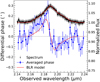 |
Fig. 1. Best-fit line profile and differential phase signal of the BLR are displayed with red curves. The Brγ profile from SINFONI spectrum is in black. The averaged differential phase data of UT4–UT2, UT4–UT1, and UT3-UT1 (see Fig. B.1) with the continuum phase subtracted are displayed in blue. |
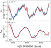 |
Fig. 2. Fitting results of (a) continuum and (b) Hβ light curves. We randomly selected 50 reconstructed continuum light curves and the reverberated Hβ light curves from the posterior sample and display them in gray. The median light curves are in red. The data points are plotted in blue. |
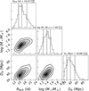 |
Fig. 3. Posterior probability distribution of the BLR radius, BH mass, and angular diameter distance of the joint analysis. The dashed lines indicate the 16%, 50%, and 84% percentiles of the of the posterior distributions. The contours indicate 1σ, 1.5σ, and 2σ. |
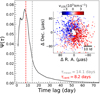 |
Fig. 4. Transfer function (Eq. (3)) of the best-fit model peaks at the time lag close to τcent, measured from the CCF method. But the mean lag (τmean) is longer because the transfer function has a long tail, which extends beyond the limit of the plot. The inset on the right displays the cloud distribution of the best-fit BLR model. The color code is the light-of-sight velocity. |
In order to assess the reliability of the uncertainties on the derived parameters, we considered the fitting process itself as well as exploring how sensitive they are to the light curve. It is possible to adjust the temperature (T ≥ 1), by which the logarithmic likelihood is divided, with CDNest in order to enlarge the uncertainty of the data when the model is not flexible enough to fit the data (Li 2018; Brewer et al. 2011). We are always able to find the clear peak of the posterior weights as a function of the prior volume with T = 1, indicating that the fitting has properly converged. The fitting results with T > 1 are consistent with those with T = 1, although the uncertainties increase. Therefore, we always report the fitting results obtained using T = 1. The measured uncertainty of the Hβ light curve is typically ∼1% of the flux, which is lower than the typical uncertainty based on the intercalibration using the [O III] doublet (Bentz et al. 2021). We fit the data with the Hβ light curve uncertainties increased to be 2% of the flux if they are smaller than the latter, and find that the results are fully consistent with those using the measured Hβ uncertainties. The uncertainty of MBH reaches 0.2 dex, while that of DA barely increases as it is dominated by the phase data. In order to further test whether the joint analysis is sensitive to the light curve measurement, we measured the Hβ light curve by decomposing the spectra with a relatively wide wavelength range (see Appendix B.3 for more details). Using the decomposition method, we measured the light curve with an approximatively 20% lower variation amplitude. We are able to obtain consistent fitting results once the nonlinear responsivity is taken into account in the joint analysis.
5. Distance and peculiar velocity of NGC 3783
Our joint analysis infers that the angular diameter distance of NGC 3783 is  Mpc. NGC 3783 has an observed redshift of 0.009730 and heliocentric velocity vh ≈ 2917 km s−1 (Theureau et al. 1998). In this section, we derive the peculiar velocity of NGC 3783, compare our measured distance with other direct and indirect methods, and discuss the uncertainty of our measurements in detail.
5.1. Peculiar velocity of NGC 3783
To correct for the motion of the Sun in the Milky Way and the peculiar motion of the Milky Way, we calculate the velocity of NGC 3783 in the frame of the Local Sheet (Tully et al. 2008; Kourkchi et al. 2020),
 (7)
(7)
where (l, b) are the Galactic longitude and latitude. The Local Sheet reference frame is a variant of the Local Group rest frame (Yahil et al. 1977; Karachentsev & Makarov 1996). Tully et al. (2008) advocated that the Local Sheet is preferable to the Local Group because it is more stable. For comparison, NGC 3783 has a Local Group velocity 2627 km s−1, according to NASA/IPAC Extragalactic Database (NED) velocity calculator. The redshift corrected for the peculiar motion of the observing frame is zls = vls/c ≈ 0.008767, which may still deviate from the cosmological redshift in the Hubble flow due to the peculiar motion of NGC 3783. Assuming (Ωm, ΩΛ, H0) = (0.3, 0.7, 70), we can infer a cosmological redshift  according to the measured DA. The peculiar velocity can be calculated (Davis & Scrimgeour 2014),
 (8)
(8)
This is very close to, albeit with large uncertainties, the peculiar velocity estimated with the Cosmicflows-3 distance–velocity calculator (see below), −182 km s−1. We also estimate the peculiar velocity using the 6dF galaxy redshift survey peculiar velocity map (Springob et al. 2014). We find 11 galaxies in the 6dF peculiar velocity catalog within 8h−1 Mpc centered on the position of NGC 3783. We averaged their peculiar velocities and uncertainties with equal weight. The estimated peculiar velocity of NGC 3783, −158 ± 43 km s−1, is consistent with the other estimates above2.
5.2. Comparison with other distance measures
Besides our measured DA, the distance of NGC 3783 can be measured “directly” with the Tully–Fisher relation (Tully & Fisher 1977) on the one hand and estimated “indirectly” with various methods relying on the large-scale structure and velocity field of the local universe on the other. Strictly speaking, these methods, as discussed below, provide the luminosity distance. Since the redshift of NGC 3783 is too low for there to be a significant difference between angular diameter distance and luminosity distance (< 2%), we do not distinguish the two in the following discussion. The direct distance measurements and indirect estimates that we discuss below are summarized in Table 2.
Distance of NGC 3783 measured with different methods.
The distance of NGC 3783 has been measured as 38.5 ± 14.2 Mpc by Tully & Fisher (1988) using the Tully–Fisher relation. This measurement was based on the magnitude of the galaxy without removing the nuclear emission from the BH accretion. This will bias the distance toward a lower value. Robinson et al. (2021) recently derived the distance of NGC 3783 to be 49.8 ± 19.6 Mpc. They derived the maximum rotational velocity measured from the newly observed H I spectrum and measured the multiband optical/NIR magnitudes of the galaxy after carefully decomposing the nuclear emission. Although they adopt a 20% uncertainty of the distance throughout the entire sample, the best-estimate distance of NGC 3783 is based on the HST photometry as the value quoted above. Nevertheless, Robinson et al. (2021) emphasized that the distance of NGC 3783 is quite uncertain mainly because the galaxy is rather face-on, leading to a large uncertainty of the maximum rotational velocity. The strong bar of NGC 3783 may also influence the rotation velocity of the galaxy (e.g., Randriamampandry et al. 2015) and affect the distance measured from the Tully–Fisher relation.
Based on the Cosmicflows-3 catalog (CF3, Tully et al. 2016) of the distance of ∼18 000 galaxies, Graziani et al. (2019) reconstruct the smoothed peculiar velocity field, for the first time, up to z ≈ 0.05 using a linear density field model. They assume a fiducial cosmology (Ωm, ΩΛ, H0) = (0.3, 0.7, 75) in the modeling while considering deviations of H0 from the fiducial value, so that the reconstructed velocity field does not depend on the assumed H0. They find the cosmic expansion is consistent with their fiducial H0 (see also Tully et al. 2016). We use the CF3 distance–velocity calculator provided by the Extragalactic Distance Database (EDD)3 to estimate the luminosity distance of NGC 3783 based on its vls corrected for cosmological effects (Davis & Scrimgeour 2014; Kourkchi et al. 2020),
![Mathematical equation: $$ \begin{aligned} { v}^\mathrm{c}_\mathrm{ls}&= { v}_\mathrm{ls} \left[1 + \frac{1}{2} (1 - q_0) z_\mathrm{ls} - \frac{1}{6} (2 - q_0 - 3 q_0^2) z_\mathrm{ls} ^2 \right], \end{aligned} $$](/articles/aa/full_html/2021/10/aa41426-21/aa41426-21-eq34.gif) (9)
(9)
 (10)
(10)
Adopting Ωm = 0.3 and ΩΛ = 0.7, we find q0 = −0.55 and NGC 3783 has  km s−14. The corresponding distance of NGC 3783 is 35.1 Mpc according to the CF3 calculator. It is not straightforward to estimate the uncertainty associated with this method. We expect that the principal source of uncertainty comes from the peculiar velocity of the galaxy due to the nonlinear effects that cannot be described by the linear model of Graziani et al. (2019). They approximate the nonlinear effects in the model with a single parameter of nonlinear velocity dispersion σNL. Taking the face value of σNL ≈ 280 km s−1 from their Bayesian inference, the linear
  of NGC 3783 is in the range 2366–2926 km s−1. The CF3 calculator yields distances ranging from 30.1 to 41.8 Mpc. Therefore, we estimate the uncertainty of the distance from the CF3 calculator is at least 6 Mpc5.
For completeness, NED provides the estimates of galaxy distances based on the multiattractor model by Mould et al. (2000). We obtain a Hubble flow velocity 2638 km s−1 after correcting for the infall due to Virgo cluster, Great Attractor, and Shapley supercluster. Taking our fiducial H0 = 70 km s−1 Mpc−1, the distance of NGC 3783 is 37.9 Mpc, very close to the result of CF3. NGC 3783 is found in a group of 9 galaxies according to an updated nearby galaxy catalog by Kourkchi & Tully (2017). The weighted distance using the 2 galaxies with measured distance from Cosmicflows-3 is 42.1 ± 5.9 Mpc. Although with considerably large uncertainty, this estimate provides an indication on the absolute uncertainty of the indirect approach.
As displayed in Fig. 5, our newly measured distance is fully consistent with the results based on other direct and indirect methods, among which the RMS scatter is ∼5 Mpc. The uncertainty of our measurement is comparable to those of the Tully–Fisher relation.
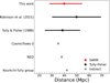 |
Fig. 5. Comparison of the distances of NGC 3783 measured with the methods listed in Table 2. The 1-σ uncertainties of direct measurements are plotted, while those of indirect measurements are not likely smaller than the former. We discuss the uncertainties of the indirect measurements in the text whenever they can be estimated. |
5.3. Statistical and systematic uncertainties
The spectral resolution of GRAVITY is moderate and noise of adjacent channels is likely correlated. This may lead to an underestimate of the inferred uncertainty. To gauge the effect of the correlated noise, we perform the analysis in two ways, (1) using only half of GRAVITY differential phase spectra (every second channel) and (2) rebinning across every two channels in the differential phase spectra. The inferred parameter uncertainties are typically ≲10% higher than those reported in Table B.1. Therefore, we conclude that the effect of the correlated phase noise is moderate6.
The relative uncertainty of our measured distance is about 33%, which is the combination of the uncertainty of the linear radius (RBLR) and the angular radius (ΘBLR) of the BLR. We find RBLR has a relatively small uncertainty of about 14%, and is mainly constrained by the RM data. In contrast, ΘBLR has about 25% uncertainty, mainly due to the relatively large uncertainty of the differential phase. The differential phase measurements have about 0.1° uncertainty per baseline, so the relative uncertainty of the ∼0.2° phase signal on three baselines is about 30%. Therefore, we find  , where δDA, δRBLR, and δϕ are the fractional uncertainties of the distance, linear radius of the BLR, and the differential phase combining 3 baselines. This is overall consistent with the conclusion of Songsheng et al. (2021) based on tests with mock data.
A primary concern in terms of systematic uncertainty is that the BLR structure of different lines measured by RM and GRAVITY may be different. A detailed comparison of Hβ and Brγ BLR structures for NGC 3783 is out of the scope of this work and will be studied in a separate paper where the velocity-resolved RM modeling will be used. Alternatively, the broad line profile contains the information of the BLR structure. Following Wang et al. (2020), we can estimate the relative size difference between the Hβ and Brγ BLRs using (q − 1)/(q + 1), where q = (FWHMHβ/FWHMBrγ)2. We measure FWHMBrγ ≈ 3680 km s−1 from our SINFONI spectrum (GC21). As introduced in more detail in Appendix B.3, we fit globally the Hβ complex of 50 RM spectra individually, including the narrow and broad components of Hβ and He II λ4686, [O III] λλ4959,5007, and Fe II emission, as well as the power-law continuum (e.g., Barth et al. 2015; Hu et al. 2015). Accounting for the instrumental broadening (Bentz et al. 2021), we find the FWHM of Hβ is stable over the RM campaign and FWHMHβ = 4341 ± 197 km s−1. Our result is slightly smaller than the FWHMHβ of the mean spectrum reported by Bentz et al. (2021) mainly due to our different approaches to fit the continuum. Therefore, the size difference between the Hβ and Brγ BLRs can be about ∼15%, which is comparable to the 13% RMS of different distance measurements (Sect. 5.2). Calculations with photoionization models will also provide useful insights (Zhang et al. 2021), although special attention needs to be paid to the difficulty of reproducing the observed flux ratios of Hydrogen lines in CLOUDY (Netzer 2020). RM observations of the same line as that observed with GRAVITY can avoid this problem.
The short time lag of NGC 3783 makes it much more straightforward to compare the BLR of different lines from RM and GRAVITY than that of 3C 273. The ∼100 day time lag of 3C 273 requires the campaign to be at least several years. The continuum light curve suffers from a further complication caused by an overall long-term trend (Li et al. 2020). In fact, the newly measured lag is about 2 times smaller than the result of early RM campaigns (Kaspi et al. 2000). The dynamical timescale of the BLR (Peterson 1993) in NGC 3783 is tdyn ≈ RBLR/vFWHM ≈ 3 years. The BLR structure likely varies on a timescale ≳tdyn (e.g., Peterson 1993; Peterson et al. 2004; Lu et al. 2016). This explains why we find that the Brγ spectra in GRAVITY measurements from 2018 to 2020 show overall consistent line profiles, and that these are also consistent with the profile from the SINFONI observation in 2019. Although it is not possible to entirely exclude it, we do not expect significant size variation in the BLR between GRAVITY and RM observations. Meanwhile, we emphasize that quasi-simultaneous observation of GRAVITY and RM within tdyn is necessary to avoid issues associated with the variability of the BLR structure.
5.4. Toward a new estimate of the Hubble constant
With a measurement of DA, one natural step forward is to estimate the Hubble constant. We derive ![Mathematical equation: $ H_0 = \mathit{v}^c_{\mathrm{ls}}/\left[D_A (1+z_{\mathrm{ls}})^2\right] = 65_{-17}^{+28}\,{{\text{ km}\,\text{ s}^{-1}}}\,\mathrm{Mpc}^{-1} $](/articles/aa/full_html/2021/10/aa41426-21/aa41426-21-eq39.gif) from the joint analysis of NGC 3783. The peculiar velocity of NGC 3783 is not included in this estimate. Our estimate (Sect. 5.1) suggests the additional systematic uncertainty introduced by the peculiar velocity is ≲10%. At this level, the differential phase errors dominate the uncertainty of H0. With upgrades to GRAVITY including adaptive optics with laser guide star and wide angle off-axis phase referencing, GRAVITY+ will allow us to observe at least several hundred suitable Type 1 AGN targets up to redshift 2–3, with Paα, Paβ, Paγ, Hα, and Hβ redshifted into K band. These lines are much stronger than Brγ with respect to the continuum. Therefore, we expect much less statistical uncertainty (e.g., ≲10%) on DA with future observations. Assuming the same sensitivity level as the current GRAVITY performance, Songsheng et al. (2021) show that it might in principle be possible to obtain a precision measurement of H0 using a large sample of differential phase and RM measurements. In practice, more effort would be necessary to address the potential bias due to the properties of different hydrogen lines and the assumptions of the BLR model.
from the joint analysis of NGC 3783. The peculiar velocity of NGC 3783 is not included in this estimate. Our estimate (Sect. 5.1) suggests the additional systematic uncertainty introduced by the peculiar velocity is ≲10%. At this level, the differential phase errors dominate the uncertainty of H0. With upgrades to GRAVITY including adaptive optics with laser guide star and wide angle off-axis phase referencing, GRAVITY+ will allow us to observe at least several hundred suitable Type 1 AGN targets up to redshift 2–3, with Paα, Paβ, Paγ, Hα, and Hβ redshifted into K band. These lines are much stronger than Brγ with respect to the continuum. Therefore, we expect much less statistical uncertainty (e.g., ≲10%) on DA with future observations. Assuming the same sensitivity level as the current GRAVITY performance, Songsheng et al. (2021) show that it might in principle be possible to obtain a precision measurement of H0 using a large sample of differential phase and RM measurements. In practice, more effort would be necessary to address the potential bias due to the properties of different hydrogen lines and the assumptions of the BLR model.
6. Conclusions
NGC 3783 is the second AGN observed by both GRAVITY interferometry and RM campaigns. We fitted both data sets simultaneously with a SARM joint analysis. The inferred model parameters are fully consistent with the previous study using only GRAVITY data, and the uncertainties of key model parameters are significantly reduced. In particular, the inferred BH mass is  (68% credible interval). For this parameter, the uncertainty is a factor of two smaller than both GRAVITY-only inference and RM measurements using the integrated Hβ light curve (dominated by the 0.3 dex calibration uncertainty of the virial factor). We also confirm the previous finding of GC21 that the BLR is highly concentrated with an extended tail of clouds out to large radius, which leads to an apparent discrepancy between the mean radius of the BLR and the measured time lag.
With the joint analysis, we are able to constrain the angular diameter distance of NGC 3783 to be  Mpc. Because NGC 3783 is in the nearby Universe, this distance can be compared to other independent direct and indirect measurements based on the Tully–Fisher relation, galaxy flow models, and its galaxy group. The BLR-based geometric distance is fully consistent with these other results. The dominant uncertainty for the distance comes from the differential phase, which has a relative uncertainty of about 30%, while the relative uncertainty from RM data is about 14%.
With the ongoing upgrade of GRAVITY, we expect to observe many AGNs with improved sensitivity. Our analysis indicates that the uncertainties of BLR model parameters, such as ΘBLR and MBH, will be reduced as the phase uncertainty decreases. Being able to substantially reduce the statistical uncertainty of H0 looks promising by both improving the precision of individual measurements and averaging the measurements over many targets. In this context, it will be important to better understand the systematic uncertainties associated with the SARM method. Further, measuring the same broad line in K band with both RM and GRAVITY will be important for future study.
Observations were made using the ESO Telescopes at the La Silla Paranal Observatory, program IDs 0100.B-0582, 0101.B-0255, 0102.B-0667, 2102.B-5053, and 1103.B-0626.
We adopt the recession velocity, 3197 km s−1 in the CMB frame, of the galaxy group that comprises NGC 3783 (Kourkchi & Tully 2017) in order to obtain the 3-D supergalactic coordinate of NGC 3783. We adopt the typical smoothing scale, 8h−1 Mpc, to find the galaxies sharing the same large-scale structure with NGC 3783. We find it makes little difference if we weight the peculiar velocity according to their separation or not, so we average them with equal weight for simplicity. The peculiar velocity has been converted from the CMB frame (Planck Collaboration I 2020) to the Local Sheet frame in order to be compared with other estimates.
It is worth noting that  does not depend on H0 (Davis & Scrimgeour 2014). And the correction with Eq. (9) is < 1% as zls is very small.
Another calculator, NAM, based on nonlinear model of galaxies within 38 Mpc (or 2850 km s−1) is provided by EDD. However, NGC 3783 is just on the upper boundary of the NAM calculator. It yields DL = 37.5 Mpc fully consistent with that of the CF3 calculator, although the NAM result is likely much more uncertain as the nonlinear model is poorly constrained at the edge of application (Kourkchi et al. 2020). We therefore prefer the result from the CF3 calculator.
In contrast to the 2-σ credible interval used in GC20 and GC21, we report the 1-σ uncertainty level throughout this paper for the simplicity of making fair comparisons to the distance measurements with other methods. The posterior distributions of most of the key parameters have profiles close to Gaussian, so the choice of the credible interval does not affect our conclusions.
Acknowledgments
We thank the referees for their careful reading of the manuscript and their suggestions that have helped to improve the clarity of it. We thank Bradley Peterson for his helpful comments on this paper. J.S. would like to thank the important help from Yan-Rong Li and Yu-Yang Songsheng to implement and test the joint analysis model. He also thanks the useful discussion from Jian-Min Wang and the IHEP group. J.D. was supported in part by NSF grant AST 1909711 and an Alfred P. Sloan Research Fellowship. M.C.B. gratefully acknowledges support from the NSF through grant AST-2009230 to Georgia State University. A.A. and P.G. were supported by Fundação para a Ciência e a Tecnologia, with grants reference UIDB/00099/2020, PTDC/FIS-AST/7002/2020 and SFRH/BSAB/142940/2018. S.H. acknowledges support from the European Research Council via Starting Grant ERC-StG-677117 DUST-IN-THE-WIND. J.S.B. acknowledges the full support from the UNAM PAPIIT project IA 101220. P.O.P. acknowledges financial support from the CNRS ≪ Programme national des hautes Énergies ≫ and from the french space agency CNES. This research has made use of the NASA/IPAC Extragalactic Database (NED), which is operated by the Jet Propulsion Laboratory, California Institute of Technology, under contract with the National Aeronautics and Space Administration. This research made use of ASTROPY, (http://www.astropy.org) a community-developed core Python package for Astronomy (Astropy Collaboration 2013, 2018), NUMPY (Van Der Walt et al. 2011), SCIPY (Jones et al. 2001), and MATPLOTLIB (Hunter 2007)
References
- Anderson, L., Aubourg, É., Bailey, S., et al. 2014, MNRAS, 441, 24 [Google Scholar]
- Astropy Collaboration (Robitaille, T. P., et al.) 2013, A&A, 558, A33 [NASA ADS] [CrossRef] [EDP Sciences] [Google Scholar]
- Astropy Collaboration (Price-Whelan, A. M., et al.) 2018, AJ, 156, 123 [Google Scholar]
- Bailey, J. A. 1998, in Optical Astronomical Instrumentation, ed. S. D’Odorico, SPIE Conf. Ser., 3355, 932 [Google Scholar]
- Baldwin, J. A. 1977, ApJ, 214, 679 [NASA ADS] [CrossRef] [Google Scholar]
- Baldwin, J., Ferland, G., Korista, K., & Verner, D. 1995, ApJ, 455, L119 [NASA ADS] [Google Scholar]
- Barth, A. J., Bennert, V. N., Canalizo, G., et al. 2015, ApJS, 217, 26 [NASA ADS] [CrossRef] [Google Scholar]
- Batiste, M., Bentz, M. C., Raimundo, S. I., Vestergaard, M., & Onken, C. A. 2017, ApJ, 838, L10 [CrossRef] [Google Scholar]
- Bentz, M. C., Walsh, J. L., Barth, A. J., et al. 2010, ApJ, 716, 993 [Google Scholar]
- Bentz, M. C., Denney, K. D., Grier, C. J., et al. 2013, ApJ, 767, 149 [Google Scholar]
- Bentz, M. C., Street, R., Onken, C. A., & Valluri, M. 2021, ApJ, 906, 50 [Google Scholar]
- Bessel, F. W. 1838, MNRAS, 4, 152 [NASA ADS] [CrossRef] [Google Scholar]
- Bhardwaj, A. 2020, JApA, 41, 23 [NASA ADS] [Google Scholar]
- Bonnet, H., Conzelmann, R., Delabre, B., et al. 2004, in Advancements in Adaptive Optics, eds. B. L. Ellerbroek, & R. Ragazzoni, SPIE Conf. Ser., 5490, 130 [NASA ADS] [CrossRef] [Google Scholar]
- Boroson, T. A., & Green, R. F. 1992, ApJS, 80, 109 [Google Scholar]
- Braatz, J. A., Reid, M. J., Humphreys, E. M. L., et al. 2010, ApJ, 718, 657 [NASA ADS] [CrossRef] [Google Scholar]
- Brewer, B. J., Pártay, L. B., & Csányi, G. 2011, Stat. Comput., 21, 649 [Google Scholar]
- Clavel, J., Reichert, G. A., Alloin, D., et al. 1991, ApJ, 366, 64 [NASA ADS] [CrossRef] [Google Scholar]
- Collier, S., Horne, K., Wanders, I., & Peterson, B. M. 1999, MNRAS, 302, L24 [NASA ADS] [CrossRef] [Google Scholar]
- Dalla Bontà, E., Peterson, B. M., Bentz, M. C., et al. 2020, ApJ, 903, 112 [CrossRef] [Google Scholar]
- Davis, T. M., & Scrimgeour, M. I. 2014, MNRAS, 442, 1117 [NASA ADS] [CrossRef] [Google Scholar]
- Du, P., & Wang, J.-M. 2019, ApJ, 886, 42 [NASA ADS] [CrossRef] [Google Scholar]
- Du, P., Lu, K.-X., Zhang, Z.-X., et al. 2016, ApJ, 825, 126 [CrossRef] [Google Scholar]
- Du, P., Zhang, Z.-X., Wang, K., et al. 2018, ApJ, 856, 6 [NASA ADS] [CrossRef] [Google Scholar]
- Eisenhauer, F., Abuter, R., Bickert, K., et al. 2003, in Instrument Design and Performance for Optical/Infrared Ground-based Telescopes, eds. M. Iye,& A. F. M. Moorwood, SPIE Conf. Ser., 4841, 1548 [CrossRef] [Google Scholar]
- Eisenstein, D. J., Zehavi, I., Hogg, D. W., et al. 2005, ApJ, 633, 560 [Google Scholar]
- Elvis, M., & Karovska, M. 2002, ApJ, 581, L67 [NASA ADS] [CrossRef] [Google Scholar]
- ESA 1997, ESA Special Publication, 1200 [Google Scholar]
- Fausnaugh, M. M., Grier, C. J., Bentz, M. C., et al. 2017, ApJ, 840, 97 [NASA ADS] [CrossRef] [Google Scholar]
- Ferland, G. J., Chatzikos, M., Guzmán, F., et al. 2017, Rev. Mex. Astron. Astrofis., 53, 385 [NASA ADS] [Google Scholar]
- Fonseca Alvarez, G., Trump, J. R., Homayouni, Y., et al. 2020, ApJ, 899, 73 [CrossRef] [Google Scholar]
- Freedman, W. L., Madore, B. F., Hatt, D., et al. 2019, ApJ, 882, 34 [Google Scholar]
- Gaia Collaboration (Prusti, T., et al.) 2016, A&A, 595, A1 [NASA ADS] [CrossRef] [EDP Sciences] [Google Scholar]
- Gaia Collaboration (Brown, A. G. A., et al.) 2018, A&A, 616, A1 [NASA ADS] [CrossRef] [EDP Sciences] [Google Scholar]
- Gaskell, C. M., & Sparke, L. S. 1986, ApJ, 305, 175 [NASA ADS] [CrossRef] [Google Scholar]
- Glass, I. S. 1992, MNRAS, 256, 23P [NASA ADS] [CrossRef] [Google Scholar]
- Goad, M. R., & Korista, K. T. 2014, MNRAS, 444, 43 [NASA ADS] [CrossRef] [Google Scholar]
- Gravity Collaboration (Abuter, R., et al.) 2017, A&A, 602, A94 [NASA ADS] [CrossRef] [EDP Sciences] [Google Scholar]
- Gravity Collaboration (Sturm, E., et al.) 2018, Nature, 563, 657 [Google Scholar]
- Gravity Collaboration (Abuter, R., et al.) 2019, A&A, 625, L10 [NASA ADS] [CrossRef] [EDP Sciences] [Google Scholar]
- Gravity Collaboration (Amorim, A., et al.) 2020, A&A, 643, A154 (GC20) [NASA ADS] [CrossRef] [EDP Sciences] [Google Scholar]
- Gravity Collaboration (Amorim, A., et al.) 2021, A&A, 648, A117 (GC21) [NASA ADS] [CrossRef] [EDP Sciences] [Google Scholar]
- Graziani, R., Courtois, H. M., Lavaux, G., et al. 2019, MNRAS, 488, 5438 [NASA ADS] [CrossRef] [Google Scholar]
- Grier, C. J., Peterson, B. M., Pogge, R. W., et al. 2012, ApJ, 755, 60 [NASA ADS] [CrossRef] [Google Scholar]
- Grier, C. J., Peterson, B. M., Horne, K., et al. 2013, ApJ, 764, 47 [NASA ADS] [CrossRef] [Google Scholar]
- Grier, C. J., Trump, J. R., Shen, Y., et al. 2017, ApJ, 851, 21 [NASA ADS] [CrossRef] [Google Scholar]
- Herrnstein, J. R., Moran, J. M., Greenhill, L. J., et al. 1999, Nature, 400, 539 [NASA ADS] [CrossRef] [Google Scholar]
- Ho, L. C., & Kim, M. 2014, ApJ, 789, 17 [NASA ADS] [CrossRef] [Google Scholar]
- Hönig, S. F. 2014, ApJ, 784, L4 [CrossRef] [Google Scholar]
- Hönig, S. F., Watson, D., Kishimoto, M., & Hjorth, J. 2014, Nature, 515, 528 [CrossRef] [Google Scholar]
- Hu, C., Du, P., Lu, K.-X., et al. 2015, ApJ, 804, 138 [NASA ADS] [CrossRef] [Google Scholar]
- Hunter, J. D. 2007, Comput. Sci. Eng., 9, 90 [NASA ADS] [CrossRef] [Google Scholar]
- Jones, E., Oliphant, T., Peterson, P., et al. 2001, SciPy: Open Source Scientific Tools for Python [Google Scholar]
- Karachentsev, I. D., & Makarov, D. A. 1996, AJ, 111, 794 [NASA ADS] [CrossRef] [Google Scholar]
- Kaspi, S., Smith, P. S., Netzer, H., et al. 2000, ApJ, 533, 631 [NASA ADS] [CrossRef] [Google Scholar]
- Kelly, B. C., Bechtold, J., & Siemiginowska, A. 2009, ApJ, 698, 895 [Google Scholar]
- Koratkar, A. P., & Gaskell, C. M. 1991, ApJS, 75, 719 [NASA ADS] [CrossRef] [Google Scholar]
- Korista, K. T., & Goad, M. R. 2004, ApJ, 606, 749 [NASA ADS] [CrossRef] [Google Scholar]
- Kourkchi, E., & Tully, R. B. 2017, ApJ, 843, 16 [NASA ADS] [CrossRef] [Google Scholar]
- Kourkchi, E., Courtois, H. M., Graziani, R., et al. 2020, AJ, 159, 67 [NASA ADS] [CrossRef] [Google Scholar]
- Lacy, C. H. 1977, ApJ, 213, 458 [NASA ADS] [CrossRef] [Google Scholar]
- La Franca, F., Bianchi, S., Ponti, G., Branchini, E., & Matt, G. 2014, ApJ, 787, L12 [NASA ADS] [CrossRef] [Google Scholar]
- Li, Y. R. 2018, CDNest: A diffusive nested sampling code in C [Google Scholar]
- Li, Y.-R., Wang, J.-M., Ho, L. C., Du, P., & Bai, J.-M. 2013, ApJ, 779, 110 [NASA ADS] [CrossRef] [Google Scholar]
- Li, Y.-R., Songsheng, Y.-Y., Qiu, J., et al. 2018, ApJ, 869, 137 [CrossRef] [Google Scholar]
- Li, Y.-R., Zhang, Z.-X., Jin, C., et al. 2020, ApJ, 897, 18 [CrossRef] [Google Scholar]
- Lira, P., Arévalo, P., Uttley, P., McHardy, I., & Breedt, E. 2011, MNRAS, 415, 1290 [NASA ADS] [CrossRef] [Google Scholar]
- Lu, K.-X., Du, P., Hu, C., et al. 2016, ApJ, 827, 118 [CrossRef] [Google Scholar]
- Mangham, S. W., Knigge, C., Williams, P., et al. 2019, MNRAS, 488, 2780 [NASA ADS] [CrossRef] [Google Scholar]
- Martínez-Aldama, M. L., Czerny, B., Kawka, D., et al. 2019, ApJ, 883, 170 [CrossRef] [Google Scholar]
- Mould, J. R., Huchra, J. P., Freedman, W. L., et al. 2000, ApJ, 529, 786 [NASA ADS] [CrossRef] [Google Scholar]
- Netzer, H. 1975, MNRAS, 171, 395 [NASA ADS] [Google Scholar]
- Netzer, H. 2020, MNRAS, 494, 1611 [NASA ADS] [CrossRef] [Google Scholar]
- Onken, C. A., & Peterson, B. M. 2002, ApJ, 572, 746 [CrossRef] [Google Scholar]
- Pancoast, A., Brewer, B. J., & Treu, T. 2011, ApJ, 730, 139 [NASA ADS] [CrossRef] [Google Scholar]
- Pancoast, A., Brewer, B. J., & Treu, T. 2014a, MNRAS, 445, 3055 [Google Scholar]
- Pancoast, A., Brewer, B. J., Treu, T., et al. 2014b, MNRAS, 445, 3073 [Google Scholar]
- Pesce, D. W., Braatz, J. A., Reid, M. J., et al. 2020, ApJ, 891, L1 [CrossRef] [Google Scholar]
- Peterson, B. M. 1993, PASP, 105, 247 [NASA ADS] [CrossRef] [Google Scholar]
- Peterson, B. M. 2014, Space Sci. Rev., 183, 253 [NASA ADS] [CrossRef] [Google Scholar]
- Peterson, B. M., & Wandel, A. 1999, ApJ, 521, L95 [NASA ADS] [CrossRef] [Google Scholar]
- Peterson, B. M., Wanders, I., Bertram, R., et al. 1998, ApJ, 501, 82 [NASA ADS] [CrossRef] [Google Scholar]
- Peterson, B. M., Ferrarese, L., Gilbert, K. M., et al. 2004, ApJ, 613, 682 [Google Scholar]
- Petrov, R. G., Malbet, F., Richichi, A., et al. 2001, Comptes Rendus Phys., 2, 67 [NASA ADS] [Google Scholar]
- Phillips, M. M. 1993, ApJ, 413, L105 [NASA ADS] [CrossRef] [Google Scholar]
- Pietrzyński, G., Graczyk, D., Gallenne, A., et al. 2019, Nature, 567, 200 [Google Scholar]
- Planck Collaboration I. 2020, A&A, 641, A1 [NASA ADS] [CrossRef] [EDP Sciences] [Google Scholar]
- Planck Collaboration VI. 2020, A&A, 641, A6 [NASA ADS] [CrossRef] [EDP Sciences] [Google Scholar]
- Randriamampandry, T. H., Combes, F., Carignan, C., & Deg, N. 2015, MNRAS, 454, 3743 [NASA ADS] [CrossRef] [Google Scholar]
- Rees, M. J., Netzer, H., & Ferland, G. J. 1989, ApJ, 347, 640 [Google Scholar]
- Reid, M. J., Pesce, D. W., & Riess, A. G. 2019, ApJ, 886, L27 [CrossRef] [Google Scholar]
- Riess, A. G. 2020, Nat. Rev. Phys., 2, 10 [NASA ADS] [CrossRef] [Google Scholar]
- Riess, A. G., Press, W. H., & Kirshner, R. P. 1996, ApJ, 473, 88 [NASA ADS] [CrossRef] [Google Scholar]
- Riess, A. G., Macri, L., Casertano, S., et al. 2009, ApJ, 699, 539 [NASA ADS] [CrossRef] [Google Scholar]
- Riess, A. G., Casertano, S., Yuan, W., et al. 2021, ApJ, 908, L6 [NASA ADS] [CrossRef] [Google Scholar]
- Risaliti, G., & Lusso, E. 2015, ApJ, 815, 33 [NASA ADS] [CrossRef] [Google Scholar]
- Robinson, J. H., Bentz, M. C., Courtois, H. M., et al. 2021, ApJ, 912, 160 [NASA ADS] [CrossRef] [Google Scholar]
- Rybicki, G. B., & Press, W. H. 1992, ApJ, 398, 169 [CrossRef] [Google Scholar]
- Shen, Y., Horne, K., Grier, C. J., et al. 2016, ApJ, 818, 30 [NASA ADS] [CrossRef] [Google Scholar]
- Songsheng, Y.-Y., Li, Y.-R., Du, P., & Wang, J.-M. 2021, ApJS, 253, 57 [NASA ADS] [CrossRef] [Google Scholar]
- Springob, C. M., Magoulas, C., Colless, M., et al. 2014, MNRAS, 445, 2677 [Google Scholar]
- Theureau, G., Bottinelli, L., Coudreau-Durand, N., et al. 1998, A&AS, 130, 333 [NASA ADS] [CrossRef] [EDP Sciences] [Google Scholar]
- Tully, R. B., & Fisher, J. R. 1977, A&A, 500, 105 [Google Scholar]
- Tully, R. B., & Fisher, J. R. 1988, Catalog of Nearby Galaxies [Google Scholar]
- Tully, R. B., Shaya, E. J., Karachentsev, I. D., et al. 2008, ApJ, 676, 184 [NASA ADS] [CrossRef] [Google Scholar]
- Tully, R. B., Courtois, H. M., & Sorce, J. G. 2016, AJ, 152, 50 [NASA ADS] [CrossRef] [Google Scholar]
- van der Marel, R. P., & Franx, M. 1993, ApJ, 407, 525 [NASA ADS] [CrossRef] [Google Scholar]
- Van Der Walt, S., Colbert, S. C., & Varoquaux, G. 2011, Comput. Sci. Eng., 13, 22 [Google Scholar]
- Wang, J.-M., Du, P., Valls-Gabaud, D., Hu, C., & Netzer, H. 2013, Phys. Rev. Lett., 110 [Google Scholar]
- Wang, J.-M., Songsheng, Y.-Y., Li, Y.-R., Du, P., & Zhang, Z.-X. 2020, Nat. Astron., 4, 517 [NASA ADS] [CrossRef] [Google Scholar]
- Watson, D., Denney, K. D., Vestergaard, M., & Davis, T. M. 2011, ApJ, 740, L49 [CrossRef] [Google Scholar]
- Williams, P. R., Pancoast, A., Treu, T., et al. 2020, ApJ, 902, 74 [NASA ADS] [CrossRef] [Google Scholar]
- Woillez, J. M., Sol, H., Perrin, G. S., & Lai, O. 2004, in New Frontiers in Stellar Interferometry, ed. W. A. Traub, SPIE Conf. Ser., 5491, 97 [NASA ADS] [CrossRef] [Google Scholar]
- Wong, K. C., Suyu, S. H., Chen, G. C. F., et al. 2020, MNRAS, 498, 1420 [Google Scholar]
- Yahil, A., Tammann, G. A., & Sandage, A. 1977, ApJ, 217, 903 [NASA ADS] [CrossRef] [Google Scholar]
- Zhang, Z.-X., Du, P., Smith, P. S., et al. 2019, ApJ, 876, 49 [NASA ADS] [CrossRef] [Google Scholar]
- Zhang, X., He, Z., Wang, T., & Guo, H. 2021, ApJ, 914, 143 [CrossRef] [Google Scholar]
Appendix A: The model of the continuum light curve
The observed continuum light curve can be described by (Rybicki & Press 1992; Li et al. 2018),
 (A.1)
(A.1)
where the vector s is the variable component of the light curve with mean zero, Eq represents the mean flux of the light curve, and nc is the noise of the observation. E is a vector of unity with the same length of the observed light curve and q is the mean of the light curve. Assuming that the light curve is a multivariate Gaussian with covariance described by Equation (2) and the measurement uncertainties are Gaussian and uncorrelated, we can interpolate and extrapolate the light curve with a uniformly and densely sampled continuum light curve model. The observed light curve is sampled in a sparse uneven time series, t1, meanwhile the model light curve is densely sampled in a uniform time series, t2. The posterior mean and covariance of the variable component of the model light curve can be calculated,
 (A.2)
(A.2)
 (A.3)
(A.3)
where  , C12 = S(t1, t2), and C22 = S(t2, t2) are matrices calculated based on Equation (2), and superscript “T” denotes transposition. We denote the observation uncertainties as σc and the identity matrix as I. The mean and variance of the long-term average of the model light curve are,
 (A.4)
(A.4)
 (A.5)
(A.5)
Therefore, the model continuum light curve is,
 (A.6)
(A.6)
where L is the lower triangular matrix of Cs, so that Cs = LLT, xs describes the deviation of the light curve variable component from its posterior mean values, and xq describes the deviation of the long-term mean from its posterior mean value. We fit xs and xq in the joint analysis as free parameters for the continuum light curve model.
Appendix B: Model fitting results and further tests
As discussed in Sect. 2, we use the differential phase data after subtracting the continuum phase primarily due to the secondary continuum emission component according to the reconstructed image (GC21). In order to display the goodness of the fit, we display the differential phases of UT4–UT2, UT4–UT1, and UT3–UT1, averaged over the three epochs, in Fig. B.1 together with the best-fit models. The phase signal is dominated by the BLR component while the residual continuum phase is moderate. The BLR phase signal is not significantly detected in the other three short baselines.
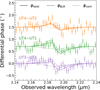 |
Fig. B.1. Averaged differential phase data (points) and the best-fit models (lines) of the three baselines that show the strongest signal of the BLR component (dashed lines). The best-fit residual continuum phases are shown with dotted lines. |
The posterior probability distributions of all of the physical parameters are shown in Fig. B.2. As discussed in Sect. 4, the posterior distributions of the BLR model of the joint analysis show very good consistency with those derived using GRAVITY data alone (GC21). The uncertainties of several key parameters, such as β, θo, i, and MBH, are reduced by a factor of ∼2, while those of the other parameters stay the same. The reduction of uncertainties of the inferred parameters is also found in the joint analysis of 3C 273 (Wang et al. 2020). This indicates that RM data help to constrain the model in a consistent manner with GRAVITY data. The β parameter is closer to the upper boundary than GRAVITY only inference, reinforcing our previous finding that the BLR is heavy-tailed. With GRAVITY data only, we found ξ peaks at ∼1 with a long tail to ∼0, indicating that ξ is not strongly constrained. With the joint analysis, ξ is even less constrained with a nearly flat posterior distribution (see Fig. B.2). This means that the fitting is not sensitive to the midplane obscuration, mainly because most of the BLR clouds (65%) are in elliptical orbits rather than radial orbits. The best-fit model favors moderate inflow, which is consistent with Bentz et al. (2021).
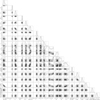 |
Fig. B.2. Posterior distribution of physical parameters from the Bayesian joint analysis. |
B.1. Constraining the BLR outer radius
We further test whether the fitting results are significantly different when we constrain the BLR inner and outer radii based on previous RM of high-ionization lines and NIR continuum. Following the discussion of GC21, we cast additional prior information that Rmin = 4 ld and Rout = 80 ld. The key results are shown in Table B.2, where DA is reduced by about 30%. The angular size of the BLR is almost the same as our primary model without additional constraints, as it is directly constrained by the GRAVITY phase data. At the same time, RBLR is reduced by about 30% due to the hard boundary Rout = 80 ld of the cloud distribution. Given the observed angular size of the BLR, a smaller DA is required in order to incorporate a smaller BLR as required by the prior. In addition, the inferred β is around 1, meaning that the cloud distribution is now exponential rather than heavy-tailed. This is because Rout limits the extent of the cloud distribution. The peak of the model differential phase is correspondingly reduced, although the model fits the data almost as well as our primary model given the data uncertainty. All of the other inferred model parameters are consistent with our primary model results. Nevertheless, the radius-constrained model is not preferred over our primary model because the inferred DA would be the smallest of the measurements discussed in Sect. 5. Quantitatively, it is about 1.5-σ lower than the other measurements, which cautions against the additional constraints to the model. While Rout = 80 ld is a reasonable choice based on NIR continuum RM analyses (Glass 1992; Lira et al. 2011), the contribution of NIR emission from the accretion disk may bias the time lag to a small value (Lira et al. 2011). Nevertheless, the joint analysis may also be biased by the assumptions of the BLR model. More comprehensive comparisons will be performed in future paper that considers different model assumptions, e.g., different cloud radial distributions and BLR size constraints.
B.2. The nonlinear response of RM
The BLR reverberates the Hydrogen ionizing (UV) photon variability from the accretion disk. The optical (i.e., V band) light curve is usually used as an approximation to the UV light curve. However, their correlation is not necessarily linear. Following (Li et al. 2018, see also Li et al. 2013), we revise Equation (3) into
 (B.1)
(B.1)
where δc captures the nonlinearity of the response. The model inference is conducted in the same way for the other parameters as discussed in Sect. 3, with the uniform prior of δc between -1 and 3 (Li et al. 2018). We find the inferred model parameters are entirely consistent with our primary fitting results (Table B.1). Some of the key parameters are listed in Table B.2. Meanwhile, the uncertainty of RBLR increases by about 70%, resulting in an increase to the uncertainty of DA by the same amount. This mainly originates from the degeneracy between δc and the scaling factor A (Equation (B.1)). Optimizing the sampling method will reduce the uncertainties of some parameters due to the degeneracy. However, this is beyond the scope of the current paper. On the other hand, the fitting of the light curve is not substantially improved. Therefore, we opt not to include the nonlinear effect of the RM response in the modeling.
Posterior median and 68% credible intervals for the BLR model parameters.
Inferred model parameters of the three tests in Appendix B.
B.3. Measuring the light curve using the decomposition method
Here we test whether the joint analysis is sensitive to the method measurement the light curve. Bentz et al. (2021) measured the Hβ flux by fitting a local linear continuum underneath the Hβ line. This method has been widely used and has been shown to be effective in producing accurate light curves for strong emission lines, such as Hβ (e.g., Peterson et al. 1998; Kaspi et al. 2000; Grier et al. 2012). Recent studies have developed methods to decompose the emission lines by simultaneously fitting various physical components to the spectra over a wide wavelength range (Barth et al. 2015; Hu et al. 2015; Shen et al. 2016). We therefore conducted a joint fit using the Hβ light curve measured with the decomposition method in order to test whether the joint analysis is sensitive to the measurement of the light curve. Following the approach of Barth et al. (2015), our model consists of the AGN power-law continuum, [O III] doublet, broad and narrow Hβ and He II lines, and the Fe II blended lines. We find the stellar continuum, reddening, and He I lines at 4471, 4922, and 5016 Å are not necessary to achieve a good fit so, to improve the stability of the decomposition of different spectra, we do not include these components. The broad and narrow emission lines are all fitted with a fourth-order Gauss–Hermite function (van der Marel & Franx 1993), whose centroid, dispersion, h3, h4, and amplitude are the parameters in the fitting. The profiles of the other narrow lines (the dispersion, h3, and h4) are tied to that of [O III] λ5007. The ratio of [O III] λλ4959,5007 is fixed to 1/3. The rest-frame wavelength separation of the two lines is fixed to 47.9 Å. The Fe II emission lines are modeled with the template from Boroson & Green (1992). We adjust the redshift, dispersion, and amplitude of the template in the fitting. We fit the spectra at rest-frame 4500–5500 Å, masking the small wavelength range of [N I] lines at 5199 and 5201 Å. We subtract all of the best-fit components except the narrow and broad Hβ line, and the Hβ flux is integrated over rest-frame 4800–4940 Å, in order to be consistent with Bentz et al. (2021). To estimate the uncertainty of the light curve, we perturb the data according to the measurement uncertainty of the spectra and redo the measurement. The final uncertainty is the quadrature sum of the statistical uncertainty from the bootstrapping and 1% of the integrated flux to make sure that the resulting uncertainty is not too small.
The light curve measured by the decomposition method has a very similar shape to that from Bentz et al. (2021) as shown in Fig. B.3. The former is about 5% higher than the latter, probably because the best-fit continuum from the decomposition method is slightly lower than that from the local continuum underneath the Hβ line. Using the method introduced in Sect. 3, we are able to infer model parameters consistent with those reported in Table B.1 within 1-σ. However, the peak-to-valley variation amplitude of the new light curve is reduced by about 20%. Correspondingly, the new inference prefers about 30–50% larger BLR radius, inclination angle, and DA in order to reduce the variation amplitude of Hβ light curve. The model inference is slightly biased in this way. To compensate for this, we need to take the nonlinearity of the Hβ response (Equation B.1) into account. This yields inferred parameters almost exactly the same as those reported in Table B.1 with the additional parameter δc ≈ −0.2. The key parameters are listed in Table B.2. The responsivity of Hβ is physically expected to be ≲1 (i.e., δc < 0) based on photoionization models (e.g., Gaskell & Sparke 1986; Korista & Goad 2004) as well as observations of e.g., NGC 5548 (Goad & Korista 2014). We emphasize that the observational effects, such as using the V-band continuum as a proxy for the ionization continuum and spectral decomposition over a wide wavelength range, may also introduce a nonlinear effect. The change of the light curve variation amplitude does not influence much the time lag of the RM. However, our test shows that the joint analysis may be biased if the nonlinear effect is not properly taken into account.
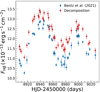 |
Fig. B.3. Comparison of the Hβ light curves measured by Bentz et al. (2021, in blue) and the decomposition method (in red, see the text). |
All Tables
Inferred median of posterior sample and central 68% credible interval for the key parameters of the analysis.
All Figures
|
Fig. 1. Best-fit line profile and differential phase signal of the BLR are displayed with red curves. The Brγ profile from SINFONI spectrum is in black. The averaged differential phase data of UT4–UT2, UT4–UT1, and UT3-UT1 (see Fig. B.1) with the continuum phase subtracted are displayed in blue. |
| In the text | |
|
Fig. 2. Fitting results of (a) continuum and (b) Hβ light curves. We randomly selected 50 reconstructed continuum light curves and the reverberated Hβ light curves from the posterior sample and display them in gray. The median light curves are in red. The data points are plotted in blue. |
| In the text | |
|
Fig. 3. Posterior probability distribution of the BLR radius, BH mass, and angular diameter distance of the joint analysis. The dashed lines indicate the 16%, 50%, and 84% percentiles of the of the posterior distributions. The contours indicate 1σ, 1.5σ, and 2σ. |
| In the text | |
|
Fig. 4. Transfer function (Eq. (3)) of the best-fit model peaks at the time lag close to τcent, measured from the CCF method. But the mean lag (τmean) is longer because the transfer function has a long tail, which extends beyond the limit of the plot. The inset on the right displays the cloud distribution of the best-fit BLR model. The color code is the light-of-sight velocity. |
| In the text | |
|
Fig. 5. Comparison of the distances of NGC 3783 measured with the methods listed in Table 2. The 1-σ uncertainties of direct measurements are plotted, while those of indirect measurements are not likely smaller than the former. We discuss the uncertainties of the indirect measurements in the text whenever they can be estimated. |
| In the text | |
|
Fig. B.1. Averaged differential phase data (points) and the best-fit models (lines) of the three baselines that show the strongest signal of the BLR component (dashed lines). The best-fit residual continuum phases are shown with dotted lines. |
| In the text | |
|
Fig. B.2. Posterior distribution of physical parameters from the Bayesian joint analysis. |
| In the text | |
|
Fig. B.3. Comparison of the Hβ light curves measured by Bentz et al. (2021, in blue) and the decomposition method (in red, see the text). |
| In the text | |
Current usage metrics show cumulative count of Article Views (full-text article views including HTML views, PDF and ePub downloads, according to the available data) and Abstracts Views on Vision4Press platform.
Data correspond to usage on the plateform after 2015. The current usage metrics is available 48-96 hours after online publication and is updated daily on week days.
Initial download of the metrics may take a while.