| Issue |
A&A
Volume 694, February 2025
|
|
|---|---|---|
| Article Number | A170 | |
| Number of page(s) | 19 | |
| Section | Extragalactic astronomy | |
| DOI | https://doi.org/10.1051/0004-6361/202453090 | |
| Published online | 12 February 2025 | |
GA-NIFS: A galaxy-wide outflow in a Compton-thick mini-broad-absorption-line quasar at z = 3.5 probed in emission and absorption
1
Centro de Astrobiología (CAB), CSIC–INTA, Cra. de Ajalvir Km. 4, 28850 Torrejón de Ardoz, Madrid, Spain
2
Kavli Institute for Cosmology, University of Cambridge, Madingley Road, Cambridge CB3 0HA, UK
3
Cavendish Laboratory – Astrophysics Group, University of Cambridge, 19 JJ Thomson Avenue, Cambridge CB3 0HE, UK
4
Università di Firenze, Dipartimento di Fisica e Astronomia, Via G. Sansone 1, 50019 Sesto F.no, Firenze, Italy
5
INAF – Osservatorio Astrofisico di Arcetri, Largo E. Fermi 5, I-50125 Firenze, Italy
6
European Space Agency, ESAC, Villanueva de la Cañada, E-28692 Madrid, Spain
7
Max-Planck-Institut für Extraterrestrische Physik (MPE), Gießenbachstraße 1, 85748 Garching, Germany
8
European Space Agency, c/o STScI, 3700 San Martin Drive, Baltimore, MD 21218, USA
9
Department of Physics, University of Oxford, Denys Wilkinson Building, Keble Road, Oxford OX1 3RH, UK
10
Department of Physics and Astronomy, University College London, Gower Street, London WC1E 6BT, UK
11
Scuola Normale Superiore, Piazza dei Cavalieri 7, I-56126 Pisa, Italy
12
Sorbonne Université, CNRS, UMR 7095, Institut d’Astrophysique de Paris, 98 Bis bd Arago, 75014 Paris, France
13
National Research Council of Canada, Herzberg Astronomy & Astrophysics Research Centre, 5071 West Saanich Road, Victoria, BC V9E 2E7, Canada
⋆ Corresponding author; mperna@cab.inta-csic.es
Received:
20
November
2024
Accepted:
18
December
2024
Context. Studying the distribution and properties of ionised gas in outflows driven by active galactic nuclei (AGN) is crucial for understanding the feedback mechanisms at play in extragalactic environments. These outflows provide key insights into the regulation of star formation and the growth of supermassive black holes.
Aims. In this study, we explore the connection between ionised outflows traced by rest-frame ultra-violet (UV) absorption and optical emission lines in GS133, a Compton thick AGN at z = 3.47. We combine observations from the James Webb Space Telescope (JWST) NIRSpec Integral Field Spectrograph (IFS) with archival Very Large Telescope (VLT) VIMOS long-slit spectroscopic data, as part of the ‘Galaxy Assembly with NIRSpec IFS’ (GA-NIFS) project.
Methods. We performed a multi-component kinematic decomposition of the UV and optical line profiles to derive the physical properties of the absorbing and emitting gas in GS133.
Results. Our kinematic decomposition reveals two distinct components in the optical emission lines. The first component likely traces a rotating disc with a dynamical mass of 2 × 10¹⁰ M⊙. The second component corresponds to a galaxy-wide, bi-conical outflow, with a velocity of ∼ ± 1000 km s−1 and an extension of ∼3 kpc. The UV absorption lines show two outflow components, with bulk velocities vout ∼ −900 km s−1 and ∼ − 1900 km s−1, respectively. This characterises GS133 as a mini-broad absorption line (mini-BAL) system. Balmer absorption lines with similar velocities are tentatively detected in the NIRSpec spectrum. Both photoionisation models and outflow energetics suggest that the ejected absorbing gas is located at 1–10 kpc from the AGN. We use 3D gas kinematic modelling to infer the orientation of the [O III] bi-conical outflow, and find that a portion of the emitting gas resides along our line of sight, suggesting that [O III] and absorbing gas clouds are partially mixed in the outflow. The derived mass-loading factor (i.e. the mass outflow rate divided by the star formation rate) of 1–10, and the kinetic coupling efficiency (i.e. the kinetic power divided by LAGN) of 0.1–1% suggest that the outflow in GS133 provides significant feedback on galactic scales.
Key words: galaxies: active / galaxies: high-redshift / quasars: absorption lines / quasars: supermassive black holes
© The Authors 2025
 Open Access article, published by EDP Sciences, under the terms of the Creative Commons Attribution License (https://creativecommons.org/licenses/by/4.0), which permits unrestricted use, distribution, and reproduction in any medium, provided the original work is properly cited.
This article is published in open access under the Subscribe to Open model. Subscribe to A&A to support open access publication.
1. Introduction
Accretion-disc outflows from active galactic nuclei (AGN) are thought to provide significant kinetic-energy feedback to their host galaxies, potentially stopping star formation and suppressing accretion onto the central black hole (e.g. Di Matteo et al. 2005; Hopkins et al. 2008; Perna et al. 2018; Giustini & Proga 2019; Bertola et al. 2024). The effectiveness of AGN feedback depends on the efficiency with which these outflows couple to the interstellar medium (ISM) in the host galaxies, an issue that remains complex and not fully understood (e.g. Harrison et al. 2017).
The study of AGN outflows often relies on the analysis of blueshifted broad absorption lines (BALs) tracing ionised gas in rest-frame ultraviolet (UV) spectra. These features are typically defined by having a full width at half maximum (FWHM) > 3000 km s−1 and velocity shifts greater than 5000 km s−1 in the AGN host galaxy rest frame (e.g. Weymann et al. 1981). Mini-BALs, narrower than BALs but still broad enough to be identified as AGN outflows, have velocity shifts between 500 and 2000 km s−1 (e.g. Hamann & Sabra 2004; Moravec et al. 2017; Hamann et al. 2019; Maiolino et al. 2024a). Even slower outflows are observed in the form of narrow absorption lines (NALs), with FWHM = 100 − 500 km s−1 and velocity offsets of a few 100 km s−1 (e.g. Vestergaard 2003; Hamann & Sabra 2004). There is no consensus about the spatial extent of UV absorption line outflows, as they trace gas along our LOS, making direct measurements of their extent impractical. Indirect methods, such as photoionisation analysis, indicate that UV outflows can reach distances ranging from tens to even thousands of parsecs (Arav et al. 2013; Xu et al. 2020). Combined, the NAL and mini-BAL outflows are more common than the well-studied BALs in AGN spectra. Specifically, ∼50% of AGN contain either NAL or mini-BAL outflows, whereas only ∼20% contain a C IV BAL outflow (e.g. Giustini & Proga 2019 and references therein).
Another approach to studying AGN outflows involves observations of rest-frame optical emission lines, which may reveal blueshifted broad wings in ionized gas tracers such as [N II] λ6583 and, more frequently, the [O III] λ5007 forbidden lines (e.g. Arribas et al. 2014; Genzel et al. 2014; Perna et al. 2015, 2019; Perrotta et al. 2019; Förster Schreiber et al. 2019; Kakkad et al. 2020; Tozzi et al. 2024). Since forbidden features can originate only from low electron density regions (i.e. ne < 106 cm−3), their broadening cannot be explained by any contamination from high density AGN broad line regions (BLR). Therefore, forbidden lines are an excellent tracer of ionised outflows, on scales extending up to several kiloparsecs from the AGN (e.g. Harrison et al. 2012; Liu et al. 2013; Cresci et al. 2023; Ulivi et al. 2024). A large fraction of AGN presents signatures of outflows in their [O III] phase, from ∼20% to ∼70%, depending on the selection criteria and outflow velocity thresholds used (e.g. Véron-Cetty et al. 2001; Mullaney et al. 2013; Perna et al. 2017; Musiimenta et al. 2023).
More generally, ejections of material from the inner regions up to the host galaxy scale can involve different gas phases, and are revealed as parsec-scale BALs (e.g. Bruni et al. 2019; Vietri et al. 2022) and ultrafast outflows (up to ∼30% of the speed of light) detected in X-rays (e.g. Pounds et al. 2003; Chartas et al. 2021; Matzeu et al. 2023), to kiloparsec-scale outflows observed in molecular, neutral, and ionised gas (e.g. Cicone et al. 2014; Lamperti et al. 2022; Mehdipour et al. 2023; Parlanti et al. 2024a; Ulivi et al. 2025). Therefore, a comprehensive characterisation of the outflow phenomena requires the use of a range of major facilities that work at different wavelengths and angular resolutions.
The need of multiple observations with different facilities have affected the direct comparison of outflows identified with different tracers, like the kinematically disturbed UV absorption- and optical emission-line components. It is not yet determined whether these phenomena are entirely distinct and are caused during different phases in the AGN fuelling and outflow life cycle, or whether they represent the same outflow episode observed with different methods, possibly depending on the inclination of the systems relative to the line of sight (LOS). In fact, individual absorption lines only reveal the outflow components along the LOS to the AGN; in contrast, optical emission lines can trace outflow emission in any direction. The literature includes only a limited number of studies that compare absorption and emission lines across AGN samples (e.g. Schulze et al. 2017; Xu et al. 2020; Ahmed et al. 2024; Temple et al. 2024; Kehoe et al. 2024).
Analyses of UV absorption and optical forbidden emission lines in individual AGN sources are also rare: there is only one integral field spectroscopy (IFS) study of two bright AGN at z ≲ 0.1 (Liu et al. 2015), and long-slit works for three individual quasars at z ≈ 2 (Tian et al. 2019; Dai et al. 2024; Stepney et al. 2024). The use of IFS observations is particularly important as they allow mapping of the ejected [O III] gas in two spatial and one velocity dimension. This capability enables direct measurement of the spatial extent of the outflows, which can only be indirectly inferred from UV absorption line analyses. In turn, this information is essential to quantify the impact these outflows have on the host galaxy.
In this paper, we present the James Webb Space Telescope (JWST) Near Infrared Spectrograph (NIRSpec) IFS and Very Large Telescope (VLT) VIMOS observations of GS133, a highly obscured AGN at z = 3.5. The NIRSpec IFS data covers the rest-frame optical ionised gas, while the VIMOS long-slit spectrum covers the rest-frame UV features. Therefore, the combination of these datasets allows us to characterise both UV and optical outflows. GS133 is located at 03:32:04.938, −27:44:31.73 in the GOODS-South field (Giavalisco et al. 2004), and is classified as an X-ray AGN in the 7 Ms exposure of the Chandra Deep Field-South (target #133 in Luo et al. 2017). Both X-ray spectroscopy fitting analysis (Luo et al. 2017) and mid-infrared diagnostics (Guo et al. 2021) identify this source as a Compton thick (CT) AGN, having a column density NH > 1.5 × 1024 cm−2 (Comastri 2004). It has an absorption-corrected 2−10 keV luminosity LX = 9 × 1043 erg s−1, an integrated luminosity from UV to infrared Lbol = 4.9 × 1045 erg s−1, a black hole mass MBH = 2 × 10⁷ M⊙, and an Eddington ratio λEdd = Lbol/LEdd = 2.4 (Guo et al. 2020). Note that because GS133 is a highly obscured AGN with no BLR emission, the BH mass was estimated assuming the MBH–M* relation with a scaling of 0.003 (Guo et al. 2021).
The paper is outlined as follows. In Section 2 we describe our JWST/NIRSpec IFS observations and data reduction, as well as the archival VLT/VIMOS data. Detailed data analysis of the optical and UV integrated spectra are reported in Sect. 3, while the NIRSpec spatially resolved spectroscopic analysis is reported in Sect. 4. Multi-wavelength diagnostics are discussed in Sect. 5. The calculation of the dynamical mass of the GS133 host galaxy is provided in Sect. 6, followed by an analysis of the outflow energetics in Sect. 7, which incorporates photoionisation and 3D gas kinematic models. The GS133 environment is examined in Sect. 8. A summary of our findings is presented in Sect. 9. Throughout, we adopt a Chabrier (2003) initial mass function (0.1 − 100 M⊙) and a flat ΛCDM cosmology with H0 = 70 km s−1 Mpc−1, ΩΛ = 0.7, and Ωm = 0.3. In our analysis of NIRSpec data, we use vacuum wavelengths according to their calibration. However, when discussing rest-frame optical emission lines, we quote their air wavelengths. Similarly, for VIMOS data, we use the air frame based on their wavelength calibration, but refer to rest-frame UV lines using their vacuum wavelengths, consistent with the standard pre-JWST practice.
2. Observations and data processing
2.1. NIRSpec data
GS133 was observed on September 12, 2022, under programme #1220 (PI: N. Lützgendorf), as part of the NIRSpec IFS GTO programme ‘Galaxy Assembly with NIRSpec IFS’ (GA-NIFS, e.g. Rodríguez Del Pino et al. 2024; Scholtz et al. 2024; Lamperti et al. 2024). The project is based on the use of the NIRSpec’s IFS mode, which provides spatially resolved spectroscopy over a contiguous 3.1″ × 3.2″ sky area, with a sampling of 0.1″/spaxel and a comparable spatial resolution (Böker et al. 2022; Rigby et al. 2023). The IFS observations were taken with the grating/filter pair G235H/F170LP. This results in a data cube with spectral resolution R ∼ 2700 over the wavelength range 1.7−3.1 μm (Jakobsen et al. 2022). The observations were taken with the NRSIRS2RAPID readout pattern (Rauscher et al. 2017) with 60 groups per integration and one integration per exposure, using a 4-point medium cycling dither pattern, resulting in a total exposure time of 3560 seconds.
We used v1.8.2 of the JWST pipeline with CRDS context 1105 to create a final cube with drizzle weighting. A patch was included to correct some important bugs that affect this specific version of the pipeline (see details in Perna et al. 2023a). We corrected count-rate images for 1/f noise through a polynomial fit. During stage 2, we removed all data in regions of known failed open MSA shutters. We also masked pixels at the edge of the slices (two pixel wide) to conservatively exclude pixels with unreliable sflat corrections, and implemented the outlier rejection of D’Eugenio et al. (2024). The combination of a dither and drizzle weighting allowed us to sub-sample the detector pixels, resulting in cube spaxels of 0.05″.
2.2. VIMOS data
The rest-frame UV spectrum of GS133 was observed as part of the survey ‘VANDELS: a VIMOS survey of the CDFS and UDS fields’ (McLure et al. 2018). This ESO public spectroscopic survey, conducted with the VIMOS spectrograph on the VLT, aimed to obtain ultra-deep, medium resolution, red-optical spectra of ∼2000 galaxies at 1 < z < 7.
GS133 was observed on May 28, 2017, using the MR grism and the GG475 filter, with a 1″ slit width and a slit length of 10″ oriented east-west on the sky. The total exposure time was 41 hours. This setup provides a wavelength coverage of 4800−10 000 Å with a nominal resolution R = 580, corresponding to a velocity resolution of approximately 500 km s−1. The spectroscopic analysis presented in this work takes advantage of the VANDELS DR4 fully reduced spectra (Garilli et al. 2021), downloaded from the ESO archive1.
A visual inspection of the 2-dimensional spectrum does not reveal any spatially resolved structure. Therefore, the analysis presented in this work focusses on the one-dimensional (1D) VIMOS spectrum.
3. Spatially integrated spectra
Figure 1 shows the integrated VIMOS and NIRSpec spectra of GS133. The VIMOS spectrum (blue curve) covers the 1070 − 2300 Å rest-frame wavelength range, while the NIRSpec spectrum (black curve) covers the range between 3710 and 7085 Å rest-frame; it was extracted from a circular aperture centred at the position of the AGN, with a radius r = 0.5″, which matches the width of the VIMOS slit. In this section, we analyse these spectra, and infer the integrated properties of the outflows both in the UV range, which is spatially unresolved in VIMOS data, and in optical, making use of NIRSpec IFS observations. Instead, Sect. 4 investigates the spatially resolved properties of the optical emission.
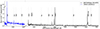 |
Fig. 1. Integrated spectrum of GS133. The blue curve identifies the VLT/VIMOS spectrum; the black line shows the JWST/NIRSpec spectrum, integrated over a circular aperture of r = 0.5″. The most prominent emission lines are marked with grey vertical lines. The gap in the middle of the NIRSpec spectrum (λrest ∼ 5400 Å) is due to the separation between the two NIRSpec detectors. |
3.1. Optical emission lines in NIRSpec cube
We fitted the most prominent gas emission lines by using the Levenberg-Marquardt least-squares fitting code CAP-MPFIT (Cappellari 2017). In particular, we modelled the Hα and Hβ lines, the [O III] λλ4959, 5007, [N II] λλ6548, 83, and [S II] λλ6716, 31 doublets with a combination of Gaussian profiles, applying a simultaneous fitting procedure, so that all line features of a given kinematic component have the same velocity centroid and FWHM (e.g. Perna et al. 2020). We used rest-frame vacuum wavelengths. Moreover, the relative flux of the two [N II] and [O III] doublet components was fixed to 2.99 and the [S II] flux ratio was required to be within the range 0.44 < f(λ6716)/f(λ6731) < 1.42 (Osterbrock & Ferland 2006). The final number of kinematic components used to model the spectra was derived on the basis of the Bayesian information criterion (BIC; Schwarz 1978).
Figure 2 shows the best-fit model around the Hβ-[O III] and Hα-[N II] regions. All emission lines exhibit a narrow core, and prominent blue and red wings. Modelling these complex profiles required four Gaussian components. The Gaussian component associated with the line cores likely traces the systemic, unperturbed emission in the GS133 host galaxy, with a broadening (velocity dispersion σ = 137 ± 5 km s−1) attributed solely to the gravitational potential of the system. In contrast, the other components likely trace a powerful outflow. Therefore, to characterise the outflow, we derived its properties from the integrated spectrum by considering the entire reconstructed profile, combining all but the narrowest and most prominent Gaussian component. This approach is justified by the potential blending of distinct (approaching and receding) outflow components that contribute to the overall profile (see Sect. 4).
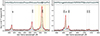 |
Fig. 2. JWST/NIRSpec integrated spectrum of GS133. The black curve identifies the integrated spectrum; the total, multi-component best-fit curve is in red, while all individual Gaussian components are shown with different colours. The fit residuals are reported in the top panels. The most prominent emission lines are marked with grey vertical lines. Light and dark yellow shaded areas in the right panel mark the [O III] emission within ±2000 km s−1 and ±1000 km s−1, respectively, from the GS133 systemic redshift. |
As the measurement of kinematic properties of emission line profiles can be obtained using different methods, depending on the specific needs and characteristics of the data, in Table 1 we reported both non-parametric velocities (e.g. Zakamska & Greene 2014), obtained by measuring the velocity v at which a given fraction of the total best-fit line flux is collected using a cumulative function, and the velocity offset Δv and velocity dispersion σ defined as the moment-1 and moment-2 measurements, respectively. Table 1 presents all velocity measurements inferred from the [O III] profile, for the reconstructed narrow and outflow components, and for the best-fit total emission line profile. Specifically, we reported the 10th-percentile (v10) and the 90th-percentile (v90) velocities of the fitted line profile, associated with the highest blueshifted and redshifted gas emission, respectively; W80, defined as v90 − v10 and representing the line width; and the velocity shift and velocity dispersion.
Properties of GS133 inferred from the optical emission lines of the NIRSpec integrated spectrum, obtained for the systemic (‘sys’), outflow (‘out’), and total (‘tot’) line profiles.
We derived the GS133 redshift from the measured wavelength of the narrow Gaussian reproducing the [O III] core emission in the integrated spectrum shown in Fig. 2: z = 3.4732 ± 0.0001. This value is roughly in agreement with previous estimates z = 3.462 (Cristiani et al. 2000) and z = 3.4739 (Balestra et al. 2010) obtained from (noisier and lower spectral resolution) ground-based rest-frame UV spectra.
The [O III] perturbed gas has a line width σout = 515 ± 3 km s−1, which is ∼4 times broader than the systemic component, and prominent blue wings extending to v < −1000 km s−1 (light-yellow region in Fig. 2). The inferred outflow velocity for the [O III] line is consistent with the general LAGN − vout trends reported in the literature (Villar Martín et al. 2020; Musiimenta et al. 2023). Specifically, it appears to be on the higher end of the distribution, suggesting slightly faster outflows compared to other sources with similar luminosities. Therefore, our results support the recent findings by Tozzi et al. (2024) showing that highly obscured and CT AGN tend to exhibit faster outflows than unobscured AGN at a given LAGN (see also Bertola et al., in prep.). A similar conclusion could be reached for another highly obscured QSO in our GA-NIFS survey, ALESS073.1, presented in Parlanti et al. (2024b). The GS133 [O III] outflow is investigated in more detail in Sect. 4.
3.2. UV lines in VIMOS spectrum
UV lines were fitted with a multi-step approach, which we summarise here. In the next section we describe our approach in full detail. First, we shifted the wavelength axis to the rest frame, using the redshift inferred from the NIRSpec data. Then, we fitted the continuum emission at > 1220 Å with a power-law, by masking all prominent line features (both in absorption and emission). Next, we normalized the continuum to 1 by dividing the original spectrum by the best-fit power-law profile. We subsequently fitted the emission lines with multi-component Gaussian profiles, and the absorption contribution with Voigt profiles. Finally, we obtained a synthetic spectrum without emission line contribution, by subtracting the best-fit emission line Gaussian profiles. This synthetic spectrum, only containing the contribution from absorption features, was finally ingested to VoigtFit (Krogager 2018), to obtain the main physical properties of the various atomic species, namely the column density and kinematics.
Because the VANDELS spectra are calibrated in air and not in vacuum, we used air wavelengths to fit the position of the different lines. The next sections describe our approach in detail.
3.2.1. Multi-component fit of emission and absorption lines
To model the low- and high-ionisation lines in the VIMOS spectrum, we used independent fits. This approach accounts for the fact that these species can trace different gas phases, potentially resulting in different systemic velocities and line widths (e.g. Shen et al. 2011; Lanzuisi et al. 2015, 2024). We classified the transitions based on their ionisation potential (IP). High-ionisation lines (HILs) were those with an IP between 30 and 80 eV, and include: N V λλ1238.82, 1242.80, Si IV λλ1393.76, 1402.77, [N IV] λ1483.32, N IV] λ1486.50, C IV λλ1548.19, 1550.77, and He II λ1640.42. Low-ionisation lines (LILs), with IP < 30 eV, included the following transitions: C II λ1334.53, Si II λ1260.42, Si III λλ1298.9, 1303.32, the fluorescent doublets C II* λλ1335.66, 1335.71 and Si II* λλ1264.74, 1265.02, and the doublet C III] λλ1906.68, 1908.73. We used single Gaussian profiles to fit the emission lines, and Voigt profiles to model the absorption line features of both HILs (N V, C IV, and Si IV) and LILs (C II, C II*, Si II*, Si III). The fitting process used the Levenberg–Markwardt least-squares fitting code CAP-MPFIT (Cappellari 2017).
To achieve better constraints on the properties of transitions with lower S/N and to reduce fit degeneracy, especially in carbon and silicon fine structure lines with potential emission and absorption contributions, we simultaneously fitted transitions within the two individual groups of HILs and LILs (e.g. Perna et al. 2015). Namely, we constrained the wavelength separation between line transitions in accordance with atomic physics (considering their air wavelengths); moreover, we fixed their widths (in km s−1) to be the same for all emission lines. For the emission line doublets C IV, N V, and Si IV, the flux ratios were allowed to vary between the optically thick (f(B)/f(R) = 1) and thin (f(B)/f(R) = 2) limits, where R and B represent the red and blue transitions of each specific doublet (e.g. Del Zanna et al. 2002). The line ratio C III] f(1907)/f(1909), sensitive to the electron density, was allowed to vary within the physical variation range 0 − 1.6 (e.g. Keenan et al. 1992). The HIL features show multiple peaks in absorption; therefore, we considered up to two kinematic components to model them. For the LILs in absorption, only one kinematic component was considered. During the fitting procedure, the flux ratio between the absorption lines of each species was treated as free parameter.
Figure 3 shows the best-fit results for both HILs and LILs. The emission lines have a consistent systemic velocity ( km s−1;
  km s−1). However, the emission line profiles are broader in HILs (
 km s−1) than in LILs (
 km s−1). Similarly, HILs in absorption are broader and require two kinematic components: the first one is blueshifted by ∼ − 900 km s−1, the second by ∼ − 2000 km s−1; both have a Doppler parameter b ∼ 400 km s−1. Conversely, LILs in absorption only require a Voigt kinematic component, blueshifted by ∼ − 900 km s−1 and with b ∼ 400 km s−1; therefore, this kinematic component perfectly match the low-velocity one identified in the HILs in absorption. These properties allow us to classify GS133 as a mini-BAL AGN.
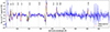 |
Fig. 3. VLT/VIMOS spectrum with best-fit results. The flux is normalised to the continuum. The blue curve identifies the integrated spectrum; the total, multi-component best fit curve is in red, while all individual Gaussian (Voigt) components are shown in yellow (green). The most prominent line transitions are marked with grey vertical lines. |
As mentioned above, the degeneracy between emission and absorption contributions may affect our results. In particular, N V, Si II, Si IV, C IV (and C II) show complex P Cygni profiles and are therefore associated with two (three) line transitions with potential contributions both in absorption and emission. Our fitting approach allowed us to reduce this degeneracy in the specific species thanks to the simultaneous modelling of other transitions like Si III, detected only in absorption, and He II and C III], detected only in emission. Nevertheless, a notable limitation is that our model does not identify any absorbing kinematic component at the systemic redshift, although such a component might exist. The combined impact of fit degeneracies and the low spectral resolution of the VIMOS data significantly constrains our ability to accurately model these complex line profiles. These limitations are further explored in the following sections.
3.2.2. Modelling of absorption lines with VoigtFit
After removing the emission line contributions inferred from the previous step, we modelled the most prominent absorption lines in the VIMOS spectrum with the Python package VoigtFit (Krogager 2018). Namely, we considered C II λ1334.53, and the N V λλ1238.82, 1242.80, Si IV λλ1393.76, 1402.77, and C IV λλ1548.19, 1550.77 doublets.
We fitted the transitions from various ions and elements simultaneously, without separating the HILs and LILs, considering two distinct kinematic components. This is justified by the fact that independent fit results presented in Sect. 3.2.1 already showed that the high and low ionisation transitions have similar profiles at the lowest velocities. Figure 4 shows the best-fit results for the four species. The LIL C II is blue-shifted by −778 ± 26 km s−1, and is symmetric, with b = 360 ± 45 km s−1. The same blue-shifted kinematic component is also detected in the three HILs; these lines, however, also required a kinematic component with more extreme properties, namely Δv = −1910 ± 50 km s−1 and b = 490 ± 80 km s−1. VoigtFit also provides a measurement of the column density for each transition and kinematic components; all best-fit parameters are reported in Table 2.
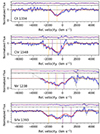 |
Fig. 4. VoigtFit models in velocity space. The normalised spectra, shown in blue with 3σ error bars, display the regions in the vicinity of the absorption lines; the best-fit models are overlaid in red. Carbon, nitrogen and silicon lines are fitted simultaneously, with two kinematic components; the vertical lines identify the velocity centroids for each kinematic component. For the doublets, the reported velocities are calculated with respect to the systemic of the blue line of the doublet; the kinematic components associated with the blue transitions are in orange, those of the red transitions are in purple. The narrow top panels show the best-fit residuals, with 3σ confidence intervals. Emission line contributions were removed prior to the VoigtFit modelling. |
To estimate a conservative lower limit to hydrogen column density NH in the outflow, we assumed no ionisation correction (e.g. N(C) = N(C IV)), and no correction for saturation. We also assumed solar abundances and the possible effects of depletion onto dust from Jenkins (2009), following Bordoloi et al. (2014). In Table 2 we report for each transition a value without correction for dust depletion (third column) and a range of values for depletion corrected densities (last column) obtained considering the range of values in Jenkins (2009, see their Table 4).
VoigtFit best-fit parameters and inferred column densities.
Overall, the column density lower limits obtained from the different species are within a narrow range of log(NH/cm−2) = 18.5 − 19.5, for both kinematic components. The main discrepancies are observed in the depletion corrected values for the Si IV transitions, which reach values up to log(NH/cm−2) = 20.6: the silicon element, however, has the largest and likely more uncertain depletion corrections, in the range [−0.22, −1.36]. Because of this, we considered in the derivation of the outflow energetics (Sect. 7) an order of magnitude approximation log(NH/cm−2) = 19. This column density is consistent with values generally associated with mini-BALs and NALs (e.g. Laha et al. 2021).
3.3. Possible Balmer absorption in the NIRSpec spectrum
The spatially integrated optical spectrum of GS133 in Fig. 2 displays two absorption features on the left side of the Hα-[N II] complex. Figure 5 shows that they are at ≈ − 1000 and ∼ − 2000 km s−1 from the Hα peak, hence broadly matching the mini-BAL features observed in the VIMOS spectrum (see Fig. 4). Therefore, these two features could be interpreted as Balmer absorption, similar to those observed in a few broad-line AGN up to z ∼ 2 in the pre-JWST era (e.g. Hutchings et al. 2002; Schulze et al. 2018; Hamann et al. 2019) and many JWST-selected Type 1 AGN (e.g. Juodžbalis et al. 2024; Kocevski et al. 2024; Matthee et al. 2024; Wang et al. 2024).
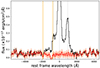 |
Fig. 5. GS133 spectrum showing tentative Balmer absorption detection in the vicinity of Hα and [N II] emission lines. The black curve shows the integrated spectrum in velocity space, with v = 0 km s−1 at the position of the Hα line. The red curve (with 1σ uncertainties in light-red) displays the residuals obtained by subtracting the best-fit Gaussian emission lines presented in Fig. 2. Two low S/N absorption features are detected close to the orange vertical lines, which mark the velocities of the mini-BAL features observed in the UV (see Table 2). |
These Balmer absorption lines are thought to originate around the edge of the obscuring torus, which is eroded and accelerated by nuclear winds; in fact, their inferred distances from the central engine are larger than the size of the BLR but smaller than the size of the dusty torus based on detailed photoionisation models using CLOUDY (e.g. Zhang et al. 2015; Shi et al. 2016; Juodžbalis et al. 2024). Alternatively, Balmer absorption could be associated with larger distances from the SMBH if the absorption is weak and the hydrogen density and NH are low (see Sect. 7.1).
However, it is important to note that the absorption features detected in the integrated spectrum of GS133 have relatively low S/N (∼2). The subtraction of emission line contributions resulted in negative flux values in some velocity channels, indicating that the absorption feature shapes may be influenced by fit degeneracies. Consequently, we did not pursue further analysis of these tentative Balmer absorption detections.
4. Spatially resolved analysis
This section presents the spatially resolved properties of the ionised gas in GS133 as inferred from the NIRSpec data-cube.
4.1. Velocity channels and spectro-astrometry
Before performing a spaxel-by-spaxel spectral fit analysis, we generated [O III] velocity channel maps and used spectro-astrometry analysis to understand if the ionised gas is spatially resolved in our NIRSpec data.
Figure 6 shows the [O III] maps obtained by integrating over three velocity ranges: [−800, −200] km s−1 to cover the high-velocity blueshifted (approaching) component, [−200, 200] km s−1 to cover the systemic emission, and [200, 800] km s−1 for the high-velocity redshifted (receding) gas. These maps show an extended morphology covering ∼1″ (7.5 kpc) along the NE to SW direction, in particular in the systemic and redshifted components; the blueshifted emission is more compact (contours identify 3σ and 5σ levels, in each panel). The NIRSpec PSF (reported in the bottom-right part of the third map) is elongated along the same NE-SW direction, roughly corresponding to the direction of the NIRSpec IFS slices (∼60°), but on smaller scales: FWHM ∼0.13″ along the slices and ∼0.1″ across the slices (D’Eugenio et al. 2024). Therefore, the [O III] emission in GS133 is spatially resolved.
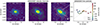 |
Fig. 6. [O III] velocity-channel maps (first-to-third panels) and spectroastrometry [O III] line positions (right panel). First to third panels: The velocity-channel maps were extracted from the ranges labelled in the individual panels. For each flux distribution, we report 3 and 5σ contour levels. The black cross identifies the GS133 nucleus, as inferred from spectroastrometry position of spectrally integrated [O III] profile (i.e. considering all velocity channels together); the white ellipse in the third panel represents the NIRSpec point spread function (PSF) at ∼2.2 μm (the [O III] observed wavelength) estimated by D’Eugenio et al. (2024); a scale bar and a compass are also reported in the first map. Right panel: Spectroastrometry of the [O III] emission, i.e. centroid positions of the line in the different velocity channels, covering a relatively small portion of the spatial extent shown in the velocity-channel maps (see white box in the third panel). The points are colour-coded by the channel velocity. The dot-dashed line roughly identifies the outflow axis, while the dotted line shows the tentative kinematic major axis of the GS133 rotating disc. |
To better understand whether the high-velocity components are spatially separated from the systemic gas in the host galaxy, we also performed a spectro-astrometry analysis. This analysis consists in determining how the centroid position of the [O III] emission changes as a function of velocity. We followed a methodology similar to that of Pereira-Santaella et al. (2018) and Lamperti et al. (2022). We binned together the velocity channels in intervals of 120 km s−1 to increase the S/N, necessary to reliably determine the position of the peak of the emission. Then, we performed a fit with the Photutils package2 to determine the peak position in each binned channel. In this way, we could determine the peak positions at sub-pixel scales.
The [O III] spectro-astrometry positions are reported in the right panel of Fig. 6. The low-velocity (|v|≤120 km s−1) channels appear oriented along the NW to SE direction, while higher velocity (|v|> 120 km s−1) are roughly perpendicular. This configuration suggests that GS133 hosts a rotating disc with a major axis perpendicular to the extended outflow (see also e.g. Fig. 3 in Lamperti et al. 2022 for a similar configuration in a nearby galaxy). The orientation of the [O III] morphological major axis, which aligns with the outflow rather than the rotational axis, suggests that outflow emission is dominant over the unperturbed gas and that a significant portion of the ejected [O III] may has relatively low projected velocities. This kinematic configuration is further investigated in the next sections.
4.2. Spaxel-by-spaxel multi-Gaussian fit
To derive spatially resolved kinematic and physical properties of ionised gas, we fitted the spectra of individual spaxels using the prescriptions already presented in Sect. 3.1. We applied the BIC selection to determine where a multiple-Gaussian fit is required to statistically improve the best-fit model. For each Gaussian component included in the fit, a S/N > 3 was required. This approach ensures that the more complex, and potentially degenerate, multiple-component fits are used only where statistically justified. In most spaxels, two Gaussian components suffice, but a few spaxels closer to the AGN position require up to four Gaussian components.
Figure 7 shows the Δv − FWHM velocity diagram obtained from our multi-Gaussian models, with the kinematic parameters of all Gaussian components required to fit the datacube. The measurements are coloured by the distance from the nucleus. Although the diagram does not show a clear trend, we note that the highest FWHMs (> 400 km s−1) are sometimes associated with significant velocity offsets (|Δv|> 150 km s−1), as observed in systems hosting AGN outflows (e.g. Woo et al. 2016; Perna et al. 2022, 2023a). In particular, the most external regions (yellow points in the figure) show a positive trend, where both velocity and FWHM increase together; the broadest components are instead blueshifted and closer to the nucleus. In contrast, the narrower Gaussian components have relatively small offsets from the zero velocity.
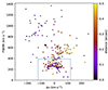 |
Fig. 7. Velocity diagram for the individual Gaussian components used to model the emission line profiles in the GS133 datacube. The measurements are coloured by the distance from the AGN. The blue lines isolate the Gaussian components with FWHM < 400 km s−1 and |Δv|< 120 km s−1 used to separate the narrow emission line kinematics (reported in Fig. 8) from the outflow kinematics (Fig. 9). |
To check for the presence of rotationally supported motions (see the right panel in Fig. 6), we selected in the Δv − FWHM plane the components with |Δv|< 120 km s−1 and FWHM < 400 km s−1 (i.e. within the blue box in Fig. 7), and constructed new datacubes containing only the systemic Hα and [O III] emission (see e.g. Perna et al. 2022 for a similar approach). The flux distribution as well as the velocity offset and dispersion of the narrow Hα and [O III] lines are reported in Fig. 8. The Δv maps display a regular pattern along the NW-SE direction, consistent with the spectro-astrometry analysis results (Sect. 4.1), with a peak-to-peak velocity shift of ∼80 km s−1. The velocity dispersion maps do not display a clear peak at the position of the nucleus, as expected for a rotating disc (e.g. Förster Schreiber et al. 2018). This could be due to the presence of the outflow and fit degeneracies. Indeed, the Δv map shows some redshifted emission towards the NE and blueshifted towards the SW (mostly in [O III]), which do not follow the rotation pattern seen in the more central regions; this component could be similarly due to a portion of the ejected gas with relatively small projected velocities. This scenario is further discussed in Sect. 7.4.
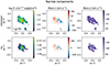 |
Fig. 8. [O III] (top) and Hα (bottom) flux, moment-1 and moment-2 maps for the systemic kinematic component. A S/N cut of 4 has been applied to generate the maps. The moment-1 maps of both lines show evidence of rotating gas in the QSO host, but neither moment-2 map shows a peak at the nuclear position (identified by a black cross). |
Figure 9 displays the flux, velocity offset, and velocity dispersion obtained for the outflow Gaussian components (outside the box identified in Fig. 7). The [O III] gas is more extended than Hα, and shows a bi-conical geometry, typical of AGN outflows (e.g. Venturi et al. 2018; Perna et al. 2022; Falcone et al. 2024). The ionised gas is blueshifted (Δv ∼ −280 km s−1) towards the NE, and redshifted (Δv ∼ 100 km s−1) towards the SW, up to ∼3 kpc. The line widths reach values as high as ∼450 km s−1 in the circum-nuclear regions, in line with the integrated fit results (Sect. 3.1).
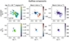 |
Fig. 9. [O III] (top) and Hα (bottom) flux, moment-1 and moment-2 maps for the outflow kinematic component. A S/N cut of 4 has been applied to generate the maps. The [O III] maps show a typical biconical outflow structure, oriented along the NE-SW direction, consistent with our spectro-astrometry analysis (Sect. 4.1). The Hα flux distribution is less extended, as this Balmer line is fainter than [O III]. |
For completeness, in Fig. A.1 we report the flux and velocity maps obtained from the total, integrated emission lines, hence without separating the systemic from the outflow components. In these maps, the signatures of the rotating disc and the bi-conical outflow configuration are less pronounced, underlining the complex kinematics in GS133.
5. Multi-wavelength diagnostics
5.1. AGN classification with optical line ratio diagnostics
We investigated the dominant ionisation source for the emitting gas across the GS133 host using the classical ‘Baldwin, Phillips & Terlevich’ (BPT) diagram (Baldwin et al. 1981). Figure 10 shows the distribution of the flux ratio diagnostics across the GS133 host galaxy extension (green-to-blue squares for increasing x- and y-axis values of the BPT diagram). The figure also shows a few spatially integrated flux ratios: the green and purple large circles refer to the systemic and outflow components obtained from the spectrum in Fig. 2; the light-blue and light-red crescent moon markers display the flux ratios of the outflow component in the integrated spectra extracted from the approaching and receding parts of the biconical outflow, respectively (using circular apertures with r = 0.15″, see inset in Fig. 10), and reported in Figs. B.1 and B.2. For reference, the BPT also displays other optical line ratio measurements from the literature, for low-z SDSS galaxies (small grey points), and star-forming galaxies and AGN at z > 2.6 recently observed by JWST (from Scholtz et al. 2023; Perna et al. 2023b; Calabrò et al. 2023), as well as the demarcation lines used to separate galaxies and AGN at z ∼ 0 from Kewley et al. (2001) and Kauffmann et al. (2003).
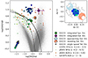 |
Fig. 10. Standard BPT diagnostic diagram. The colour-coded squares show GS133 single-spaxel measurements associated with the spatial regions shown in the top-right panel; green-to-blue colours mark increasing line ratios, as indicated with the arrow in the bottom-left part of the diagram; only spaxels with S/N > 3 in all lines are shown. The large green and purple circles display the line ratios measured from r = 0.5″ spatially integrated regions, for the systemic and outflow components, as labelled: the large crescent moon symbols refer to the outflow component line ratios measured in circular regions marked in the inset (with the same crescent moon symbols). The solid (Kewley et al. 2001) and dashed (Kauffmann et al. 2003) curves commonly used to separate purely star-forming galaxies (below the curves) from AGN (above the curves) are also reported. Finally, the BPT shows local galaxies from SDSS (Abazajian et al. 2009, indicated in grey), and additional measurements for z = 2.6 − 6.7 sources from the literature: star-forming galaxies are marked with small green symbols and refer to CEERS (Calabrò et al. 2023) and JADES (Scholtz et al. 2023) surveys, while AGN are marked with small orange symbols and refer to JADES (Scholtz et al. 2023) and GA-NIFS (Perna et al. 2023b) surveys. |
The spatially resolved line ratio measurements do not show a significant variation across the GS133 host galaxy extension, although a tentative trend can be observed. The lowest [O III]/Hβ and [N II]/Hα line ratios are observed in the outskirts of the galaxy, towards NW and SE (see the map in the inset), and are very close to the BPT locus of star-forming galaxies at high-z (green symbols in the figure). Instead, the highest line ratio measurements are along the outflow axis, likely corresponding to the AGN ionisation cones of GS133. In fact, these high line ratios are in a BPT region free from contamination by star forming galaxies at any redshift, and only populated by AGN systems (e.g. Scholtz et al. 2023; Perna et al. 2023a,b; Parlanti et al. 2024b; Decarli et al. 2024).
The spatially integrated measurements reported in the figure (large circles and crescent moon symbols) similarly indicate that the systemic narrow emission is consistent with star-formation ionisation, while the outflow components are AGN dominated (see also line ratios reported in Table 3).
Optical emission line ratios from NIRSpec integrated spectra.
In conclusion, both spatially integrated and spatially resolved line ratios support an AGN classification based on the standard BPT diagnostic diagram. In fact, while the BPT diagram may lose sensitivity in distinguishing between AGN and star-forming galaxies in low-mass, low-metallicity systems at high redshift, it remains effective for identifying AGN in more massive and metal-enriched galaxies (e.g. Z > 0.5 Z⊙, Feltre et al. 2016).
5.2. AGN classification with UV line ratio diagnostics
The direct observation of high-ionisation emission lines in the UV spectrum of GS133, such as N V λλ1239, 43, C IV λλ1548, 51, He II λ1640, also in combination with other UV transitions, can be used to obtain a further confirmation of the presence of AGN emission in this high-z source (e.g. Mascia et al. 2023; Scholtz et al. 2023; Maiolino et al. 2024b).
In Table 4 we report the main UV line ratios commonly used to distinguish between AGN and star-forming galaxies in the literature (e.g. Feltre et al. 2016; Nakajima et al. 2018; Perna et al. 2023b; Topping et al. 2024). All of these line ratios are compatible with AGN ionisation, which is consistent with the X-ray and optical BPT classifications introduced in the previous sections.
UV emission line ratios from the VIMOS spectrum.
5.3. CT AGN classification with L([O III])/L(X-ray) diagnostic
X-ray diagnostics are the most reliable methods for identifying CT AGN (e.g. Lanzuisi et al. 2017). Previous analyses by Luo et al. (2017) and Li et al. (2019) of the Chandra X-ray spectrum for GS133 suggested column densities of NH ≈ 1.5 × 1024 cm−2, which is around the threshold typically used to classify AGN as CT. However, due to the significant uncertainties associated with the low number of X-ray counts typical for high-redshift sources like GS133, where only 70.7 aperture-corrected source counts are available in the 0.5−7 keV band (Luo et al. 2017), the true column density could be lower. To strengthen the case, multi-wavelength diagnostics have been employed by Guo et al. (2021). They compared the X-ray to mid-infrared (6 μm) luminosity, commonly used to identify CT sources as the infrared emission is less affected by obscuration than X-rays; they found obscuration exceeding 1.5 × 1024 cm−2. In this section, we tested an additional diagnostic to further support the CT classification of the AGN in GS133.
Maiolino et al. (1998) provided a diagnostic based on the ratio between the observed 2−10 keV and the reddening-corrected [O III] luminosities to infer the column density of obscured AGN. Adopting their methodology, we derived a luminosity ratio log(LX/L[OIII]) = −1.4, corresponding to a lower limit log(NH/cm−2) > 2 × 1024 (see their Fig. 6). Specifically, the X-ray to [O III] luminosity ratio was calculated using the [O III] outflow luminosity reported in Table 1 (hence excluding any possible contribution from star formation). The [O III] luminosity was corrected for dust extinction considering an intrinsic Balmer decrement of 2.86 and assuming the Cardelli et al. (1989) extinction law. Therefore, this result further supports the CT nature of GS133.
6. Dynamical mass
Having an estimation of the kinematics and extent of a galaxy allows us to provide a constraint on the dynamical mass of the galaxy, Mdyn. Under the assumption that the gas is distributed in a flat disc, the dynamical mass enclosed within a radius R is Mdyn = 2.33 × 10⁵ vcirc2R M⊙, where vcirc is the circular velocity in km s−1 at a galactocentric distance R, given in kpc (Walter et al. 2004; Neeleman et al. 2021; Perna et al. 2022). Since we could only marginally resolve the disc structure in GS133, we assumed an extent of R = 1 kpc, typical of z = 3 − 4 galaxies (Kartaltepe et al. 2023; Costantin et al. 2024), and that the FWHM (i.e. 2.355 × σ) of the systemic Hα line can be used as a proxy for the circular velocity, so that vcirc = 0.75 FWHM/sin(i) = 300 km s−1, assuming a mid-range inclination of 55° following, for instance, Neeleman et al. (2021) and Decarli et al. (2018).
Under these assumptions, the dynamical mass of GS133 is Mdyn = 2 × 10¹⁰ M⊙, broadly consistent with the stellar mass inferred by Guo et al. (2020) and Circosta et al. (in prep.) from spectral-energy-distribution (SED) analysis: M* = 5 × 10⁹ M⊙, and 3 × 10¹⁰ M⊙, respectively. The difference in stellar mass estimates can be explained by the common degeneracy between AGN and stellar components in the optical and UV regime (e.g. Ciesla et al. 2015). A more comprehensive comparison of the SED fitting results will be provided in Circosta et al. (in prep.).
7. Outflow properties
In this section we measure the mass rate and energetics of the ionised outflow as inferred from the blueshifted outflow components of absorbing (C II, C IV, and N V) and emitting (Hβ and [O III]) line transitions. We begin with standard assumptions commonly used in the literature, then refine these measurements by applying detailed photoionisation modelling for the absorption lines and 3D kinematic modelling for the emission lines. We also compare our results with outflow model predictions and general AGN properties to exclude less plausible assumptions, aiming to derive more accurate outflow properties for both the absorbing and emitting gas.
7.1. Energetics of absorbing gas outflow
We measured the mass rate of the absorbing outflow gas as inferred from the blueshifted mini-BAL components of C II, C IV, and N V. Following Bordoloi et al. (2014), we assumed for simplicity a thin-shell approximation (Ω = 4π), and maximised to unity the angular and clumpiness covering factors (CΩCf = 1):
where NH is the hydrogen column density and Rout and vout are the mini-BAL galactocentric radius and velocity, respectively. The kinetic power of the absorbing material can be derived from the relation Ė = 1/2Ṁv2:

(see also Hamann et al. 2019). We assumed that the absorbing outflow is related to the two distinct components travelling at different velocities (Fig. 4), and that vout is approximated by the velocity shift Δv of a given component, hence ∼ − 800 km s−1 and ∼ − 1900 km s−1 (Table 2). For the extent of the mini-BAL outflow, we initially used a range of values between 1 pc and 10 kpc (following Dunn et al. 2010; Saturni et al. 2016; Moravec et al. 2017; Bruni et al. 2019), as it cannot be inferred without knowing the hydrogen density in the absorbing ejected gas. For the column density estimate, we considered median values inferred from dust-depletion corrected NHc reported in Table 2, excluding the Si IV estimates as they are associated with more uncertain corrections (see Jenkins 2009): 8 × 1018 cm−2 and 1 × 1019 cm−2 for the low- and high-velocity outflows, respectively. We obtained Ṁ(Abs) = 0.003 − 30 M⊙ yr−1 and Ė(Abs) = (0.0004 − 4) × 1043 erg s−1, considering the extremely large range of possible values for Rout, and computing the sum of the contributions from two kinematic components (with ∼70% coming from the faster and denser component). In the next subsection, these measurements are refined taking into account detailed photoionisation models.
7.2. Photoionisation modelling for ejected absorbing gas
To infer the physical conditions within the mini-BAL, we computed a series of simulations using the photoionisation code CLOUDY (c17.03; Ferland et al. 2017) and compared them with observations. We set up a series of 1D single-cloud models with the ionising SED set to a CLOUDY built-in multi-component AGN spectrum described by the following formula

Specifically, we set the cut-off temperature for the accretion disc to TBB = 106 K, the optical-to-X-ray ratio to αox = −1.4, the X-ray slope to αX = −1, and the UV slope to αuv = −0.5 (by adjusting parameter a in the equation above). The SED we adopted roughly reproduces the shape of the observed UV continuum observed by VLT/VIMOS. For the absorbing clouds, we explored a wide range of ionisation parameters3, U, from 10−4.5 to 1. We set the clouds to be isobaric and vary the density in a range of 1 ≤ log(nH/cm−3)≤7. All models are computed until a cumulative hydrogen column density of NH = 1022 cm−2, and cumulative column densities for different atomic/ionic transitions as functions of depth are saved individually for the search of solutions that match the derived values for GS133. For the chemical abundances, we adopted the solar abundance set of Grevesse et al. (2010) and set the ratio N/C as a free parameter to account for variations due to chemical enrichment history (Maiolino & Mannucci 2019). Finally, since Si is usually highly depleted onto dust grains in the ISM (e.g. Jenkins 2009), we set Si/C as an additional free parameter to probe the level of dust depletion.
We considered separate models for the two kinematic components at −800 km s−1 and −1900 km s−1. We used a single-cloud model, where both C II and C IV can be found, but C IV absorption happens in the more inner region of the cloud due to its higher ionisation potential. This means that when C II has reached a large column density at a certain depth in the cloud, the column density of C IV usually has already reached its maximum value. The stopping conditions for the cumulative density at NH = 1022 cm−2 ensure that we match the values inferred from the VIMOS spectrum for both C II and C IV. Specifically, for the low-velocity component, we searched for models with column densities of the C II that match our derivations from the analysis of the VIMOS spectrum. Then, we allowed the column density of C IV to differ from the measured value by ±0.15 dex (i.e. 3σ, Table 2), and scaled the N/C and Si/C abundances to reproduce the column densities measured for N V and Si IV transitions. We also performed a minimum χ2 search using the measured column densities for the above transitions and obtained consistent results.
In Fig. 11 we show the best-fit nH and NH for the absorbing gas. For the mini-BAL component with vout ∼ −800 km s−1, we found low-density models with log(NH/cm−2) = 20.2−20.3, log(nH/cm−3) = 1−2, and log(U) in the range [−2.7, −2.6] can well reproduce our measurements. High-density models with log(nH/cm−3) = 4−5 also have a good match with our measurements. All these models require a high log(N/C) = 1 to reproduce N V absorption, consistent with CNO equilibrium ratio in asymptotic giant branch (AGB) stars (Maeder et al. 2015). However, since there is no strong nebular emission of N IV] and N III] in the VIMOS spectrum, we caution the interpretation of the high N/C. As an alternative explanation, due to the high ionisation potential of N V, N V absorption might actually occur in a separate density-bounded cloud closer to the central AGN, which cannot be described with single-cloud models; fit degeneracy between emission and absorption contributions could also explain the high N/C. Based on the best-fit Si/C, we inferred a depletion factor of 0.52 dex for the Si IV. The depletion of Si IV is consistent with a moderate amount of dust depletion found in the compilation of MW sightlines by Jenkins (2009) with a unified depletion strength of F* = 0.25. In comparison, a stronger depletion strength of F* = 0.5 is typical for star-forming galaxies at z ≲ 0.1 (Gunasekera et al. 2023). For the high-velocity component, we found low-density models with log(NH/cm−2) = 19.4−19.6, log(nH/cm−3) = 1.5−3.0, and log(U) in the range [−2.8, −2.7] can reproduce our measurements if we leave N/C and Si/C as free parameters. There is a high-density solution at log(nH/cm−3) ≈ 6 as well. If we further constrain N/C and Si/C in the models to the values obtained for the slow component, the preferred models for the fast component would have log(NH/cm−2) ≈ 19.6, log(nH/cm−3) = 2.0−4.0, and log(U) in the range [−2.8, −2.7].
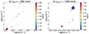 |
Fig. 11. Hydrogen densities and column densities predicted by CLOUDY photoionisation models for the two mini-BAL components. Only models with χ2 < 5 are shown and the sizes of the symbols are inversely scaled with χ2. In addition, models are colour coded according to their ionisation parameters. Both outflow components have low-density and high-density solutions, although the high-density solution would imply extremely thin layers of gas. |
For both low- and high-velocity components, our low-density models suggest that the effective thickness of the absorbing gas (i.e. NH/nH) can span a range from 4 to 0.04 pc if it has a volume filling factor close to unity, consistent with previous results for low-z systems from the literature (e.g. Choi et al. 2022). In comparison, high-density solutions correspond to physical scales of 6 × 10⁻⁴ − 10−3 pc for the low-velocity component and 10−5 pc for the high-velocity component.
Knowing the hydrogen density and ionisation parameter for the cloud from CLOUDY models, we could also infer the distance of the absorbing material from the SMBH, from
where Q is the number of ionising photons per unit time, proportional to the AGN bolometric luminosity (see e.g. Eq. 4 in Baron & Netzer 2019), and c is the speed of light. By solving this equation for Rout, we obtained distances of 1−10 kpc for the two kinematic components with low-density CLOUDY models reported above. We note that much smaller distances would require significantly higher densities of nH (≈106 cm−3), which, however, would be associated with an unphysical thickness of the cloud, orders of magnitude smaller than typical dimensions of a single cloud in the BLR (≲10−3 pc), and smaller than normally assumed in BAL models (e.g. r ∼ 0.3 − 3 pc in Ishibashi et al. 2024). These considerations favour the low-density models as the most plausible.
Therefore, our CLOUDY models suggest that the mini-BAL material in GS133 is at the same distance of emitting gas and not confined in the nuclear (parsec-scale) regions. While single-cloud models might be overly simplistic for a system like GS133, which exhibits multiple kinematic components in both low- and high-ionisation lines, as well as an extended, bi-conical [O III] outflow, more complex models with multiple clouds would introduce greater degeneracies (as they require the modelling of > 10 line transitions; e.g. Marconi et al. 2024). Therefore, our approach represents a compromise, providing indicative properties of the mini-BALs in GS133.
Using the best-fit CLOUDY parameters, we recalculated the UV outflow energetics. For the low-velocity component, we found mass outflow rates of 14−140 M⊙ yr−1 and kinetic powers of (5−50) × 1042 erg s−1, with the range reflecting an outflow extent from 1 to 10 kpc. For the high-velocity component, the corresponding values are 6−60 M⊙ yr−1 and (1−10) × 1043 erg s−1, with the same range for the outflow extent.
7.3. Energetics of emitting gas outflow
We computed the mass outflow rate of the ionised gas as inferred from the blueshifted outflow component of Hβ, assuming a simplified biconical outflow distributed out to a radius Rout, following Cresci et al. (2015):
where L41(Hβ) is the Hβ luminosity associated with the outflow component in units of 1041 erg s−1 (corrected for dust extinction), ne is the electron density in cm−3, and vout is the outflow velocity in km s−1.
For comparison, we also computed the mass outflow rates employing the [O III] luminosity and assuming the same geometrical configuration:
![$$ \begin{aligned} \dot{M}_{\mathrm{out}}(Em,\,\mathrm{[OIII]}) = 0.5 \times \frac{L_{41}(\mathrm{[OIII]})\,v_{\mathrm{out}}}{n_{\rm e}\ R_{\mathrm{out}} 10^\mathrm{[O/H]}}\,M_{\odot }\,\mathrm{yr^{-1}}, \end{aligned} $$](/articles/aa/full_html/2025/02/aa53090-24/aa53090-24-eq43.gif)
where L41([O III]) is the [O III] luminosity associated with the outflow component in units of 1041 erg s−1 (corrected for dust extinction), and 10[O/H] is the metallicity of the outflowing gas in solar units (see also Cano-Díaz et al. 2012). The kinetic power of the ejected emitting gas can be derived as Ė = 1/2 Ṁv2:
For simplicity, the outflow energetics of the emitting gas were derived assuming a simple single-radius wind, because of the unknown detailed geometrical configuration of the outflow (i.e. opening angles and inclinations of the conical structures, deprojected sizes and velocities). The fact that the gas is ionised by the AGN did not allow us to derive metallicity measurements for the outflowing gas, but the high [N II]/Hα line ratio (> 0.3) and stellar mass of the system (∼1010 M⊙) allows us to reasonably assume a solar metallicity to derive [O III]-based outflow energetics. We also assumed an outflow extension of 3 kpc, and an outflow velocity vout = 1000 km s−1 for both [O III] and Hβ, as order of magnitude estimates (based on the observed distribution of high-v [O III] gas in Fig. 6, and our multi-Gaussian fit decomposition results reported in Table 1). Similarly, we assumed an electron density ne = 1000 cm−3, considering that we could not obtain a measurement for the ejected gas because of the faintness and complexity of the [S II] profiles, and the extremely high density derived from the narrow [S II] components (3300 ± 500 cm−3) in the integrated spectrum shown in Fig. 2. With these assumptions, we obtained Ṁout([O III]) = 60 M⊙ yr−1 and Ṁout(Hβ) = 200 M⊙ yr−1, respectively4. We note that the [O III]-based estimates are a few times lower than those obtained with Hβ, in agreement with previous results suggesting that [O III] provides a lower limit on the ionised gas mass (see e.g. Carniani et al. 2015; Perna et al. 2015; Marshall et al. 2023; Venturi et al. 2023). Therefore, in the following, we refer only to the Hβ-based outflow energetics for the emitting gas component of the GS133 outflow. The inferred outflow mass rate, kinetic power, and momentum power (defined as Ṗ = Ṁv), are reported in Table 5. In Sect. 7.5 we compare these quantities with the AGN bolometric luminosity and some theoretical predictions to infer the driving mechanisms of the mini-BAL and [O III] outflows detected in GS133.
Mini-BAL and [O III] outflow energetics.
7.4. 3D modelling of the outflowing emitting gas
Our CLOUDY models suggest that the mini-BAL absorbing material, traced by C II, C IV, and other atomic species detected in the VIMOS spectrum of GS133, extends to kpc scales. Since we observe the mini-BAL directly along the LOS, we aim to determine whether this absorbing outflow is partially mixed with the emitting [O III] gas.
Despite the fact that the [O III] outflow in GS133 extends over kiloparsec-scales, it only covers a few tens of spaxels in the NIRSpec cube (Fig. 9). A detailed reconstruction of the 3D geometry of the outflow, as done for targets at lower redshifts (e.g. Meena et al. 2021; Cresci et al. 2023; Ulivi et al. 2025), would require finer spatial sampling and higher angular resolution than what NIRSpec IFS provides. Nonetheless, we used our framework ‘Modelling Outflows and Kinematics of AGN in 3D’ (MOKA3D; Marconcini et al. 2023) to test whether our NIRSpec data are compatible with the presence of a biconical outflow where the approaching side intersects our LOS.
For simplicity, we adopted constant radial velocity profiles for both the approaching and receding components of the [O III] outflow. We also assumed a bi-conical geometry, with a semi-aperture angle of 45°, consistent with other AGN-driven outflows studied at lower redshifts (e.g. Fischer et al. 2014; Müller-Sánchez et al. 2016; Meena et al. 2021; Perna et al. 2022). For the approaching cone, we required an inclination angle with respect to the LOS in the range [−45°, +45°], to ensure the overlap with our LOS; for the receding cone, we required an inclination angle in the range [180° −45°, 180° +45°].
The [O III] outflow is reproduced with MOKA3D with an approaching cone with an inclination angle of 40° with respect to the LOS, a position angle of 50°5, and an intrinsic deprojected outflow velocity of 900 km s−1; the receding cone has an inclination angle of 225°, a position angle of 230°, and an intrinsic deprojected outflow velocity of 800 km s−1. The two cones extend out to 5 kpc. Figure 12 shows the 3D representation of the outflow, together with the flux, velocity, and velocity dispersion maps from data, the 3D model, and the residuals; the figure indicates the MOKA3D capabilities in recovering the general properties of [O III] outflowing gas with a bi-conical model. In particular, a hollow conical best-fit model is obtained, consistent with many other AGN-driven outflows reported in the literature (e.g. Marconcini et al. 2023 and references therein). We also note that the MOKA3D model necessitates the presence of emission on kiloparsec scales located close to the plane of the sky. This component exhibits relatively low projected velocities and can explain the slightly redshifted emission observed towards the NE and the blueshifted emission towards the SW in the narrow component maps shown in Fig. 8 which cannot be attributed to a rotating pattern.
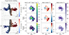 |
Fig. 12. MOKA3D model (left) and moment maps from NIRSpec data and MOKA3D model (right panels). In the 3D representations of the GS133 outflow structure, the XY represents the plane of the sky, while Z axis is the LOS. The observer is positioned on the left, and sees as blueshifted (redshifted) all the approaching (receding) gas, according to the colour bar; largest bubbles identify brightest clumps. The three-by-three panels show the comparison between the flux, Mom-1 and Mom-2 maps of [O III] (top panels) and MOKA3D model (middle panels) for the GS133 bi-conical outflow. The bottom panels present the residuals obtained subtracting the model from the data. |
From this simple MOKA3D model, we can derive two main results. On the one hand, the [O III] gas appears to share the same velocity as the low-velocity component in C II, C IV, and other UV lines (|v10out|∼vMOKA ≈ 900 km s−1); this suggests that both the absorbing gas and part of the emitting [O III] could lie along our LOS and may be associated with the same outflow, possibly even physically mixed. On the other hand, the second kinematic component detected in absorption in C IV and other HILs moves at vout ∼ −1900 km s−1 (see Fig. 4); this component is not detected in the ionised emitting gas, and could therefore have slightly different physical (e.g. composition, ionisation state) or structural (e.g. spatial location) properties. Alternatively, this very high-velocity component may be too faint to be detected in emission.
7.5. Physical mechanisms for the wind propagation
We compared our inferred values of the total outflow kinetic power with the AGN bolometric luminosity and the expected kinetic power ascribed to stellar processes. The AGN bolometric luminosity can be constrained from the X-ray emission, applying a Duras et al. (2020) bolometric correction of 260 to the absorption corrected 2−10 keV luminosity from Li et al. (2019), Lbol = 1.6 × 1045 erg s−1. This value is broadly consistent with the SED-based AGN luminosity inferred by Guo et al. (2021, Lbol = 4.9 × 1045 erg s−1), and by Circosta et al. (in prep., 2 × 1045 erg s−1). However, these values are significantly lower than those inferred from the outflow component of the optical emission lines: from Hβ flux, applying the Netzer (2019) bolometric correction, Lbol(Hβ) = 4.5 × 1046 erg s−1, and from [O III] flux, applying the Heckman et al. (2004) correction, Lbol([O III]) = 3 × 1046 erg s−1 (even higher values would be obtained applying a dust extinction correction, and considering the total line profiles, which however could be contaminated by star-formation processes). Since the X-ray-based value is in between those from the SED analysis, in the following, we refer to the former as our fiducial estimate.
The kinetic power associated with the optical outflow is 3 × 1042 erg s−1, hence ∼0.2% of the radiative luminosity of the AGN, consistent with the energetics of other AGN in the literature (e.g. Harrison et al. 2018). Comparable values can be obtained for the mini-BAL considering a kiloparsec-scale extension: Ėout/Lbol ∼ 0.1% for Rout = 1 kpc, and ∼1% for Rout = 10 kpc.
Following Veilleux et al. (2005), we assumed an expected kinetic power ascribed to stellar processes proportional to the SFR (20 M⊙ yr−1, from Guo et al. 2020, < 70 M⊙ yr−1, from Circosta et al., in prep.), and concluded that the outflow kinetic power of the emitting gas cannot be associated with star formation driven winds, as they would require an extreme coupling between the stellar processes and the observed winds, of the order of ≈100% or more.
The momentum power inferred for the optical emitting gas is ṖHβ = 1 × 1036 dyne, with a momentum rate ṖHβ/(Lbol/c) = 24. For the UV absorbing gas, we obtained (2 − 20)×1035 dyne, resulting in ṖUV/(Lbol/c) = 4 − 40, with lowest values occurring for a mini-BAL with Rout = 1 kpc and highest for Rout = 10 kpc (still compatible with measurements of other AGN in the literature, see e.g. Fig. 3 in Bischetti et al. 2024).
A momentum flux rate obtained under the assumption of a very compact mini-BAL is far smaller than the moment flux rate of the Hβ outflow (ṖUV/(Lbol/c) = 0.004 for Rout = 1 pc), and hence than what is expected for a momentum conserving wind (e.g. Fiore et al. 2017). If the AGN outflow is energy conserving, it is possible that the mini-BAL is radiatively launched with small momentum flux in the nucleus, and then boosted to ṖHβ/(Lbol/c)∼24 at larger distances (e.g. Faucher-Giguère & Quataert 2012). However, such a dramatic increase in momentum flux, by four orders of magnitude, is highly uncommon (see Fig. 8 in Tozzi et al. 2021). This further supports our CLOUDY model results indicating that the mini-BAL is located at kpc scales.
Summarising, the computation of outflow energetics allowed us to obtain an independent (but still indirect) confirmation of the kiloparsec-scale location of the mini-BAL; the modest momentum bursts inferred for optical and UV transitions, of the order of 2 to 40, are more likely compatible with energy conserving winds rather than momentum driven ones (e.g. King & Pounds 2015), also taking into account that with current data we cannot probe the neutral and molecular outflow phases which could significantly contribute to the outflow energetics on kiloparsec-scales (e.g. Brusa et al. 2018; Cresci et al. 2023; Davies et al. 2024; D’Eugenio et al. 2024).
8. Environment
NIRSpec IFS data do not reveal any close companions or line emitters around GS133, in contrast with several z > 3 AGN and QSOs recently observed with JWST, many of which show multiple nearby companions (e.g. Wylezalek et al. 2022; Marshall et al. 2023, 2024; Perna et al. 2023a,b; Übler et al. 2023, 2024a,b; Kashino et al. 2023; Yang et al. 2023). Available JWST/NIRCam images (programme ID 3990, PI: T. Morishita) show some extended emission towards E-SE associated with the GS133 host, possibly indicating merger features or a disturbed morphology, and faint compact sources outside of the NIRSpec FOV. Figure 13 shows the composite F115W/F200W/F444W cutout, highlighting the GS133 extended features. However, these faint features remain undetected in the spectroscopic data, which are too shallow (≲1 h-integration) in comparison with NIRCam imaging (e.g. 6 h-integration in the red band F444W).
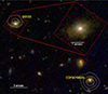 |
Fig. 13. JWST/NIRCam F115W/F200W/F444W cutout showing the close environment of GS133. The red dashed box marks the NIRSpec IFS FOV, while the white contours show the Chandra 0.5–7 keV emission from Luo et al. (2017), highlighting the position of two X-ray AGN with a projected separation of ∼130 kpc and a velocity offset of ∼5000 km s−1 (Δz = 0.08). The apparent offset between the NIR and X-ray positions can be attributed to Chandra’s low angular resolution and the fact that the Chandra image is composed of multiple observations taken with varying aim points and roll angles. The inset shows a zoom-in on GS133. The images are oriented north up, east left. |
Interestingly, GS133 is located near another AGN, identified as CDFS019505 (in the bottom right of Fig. 13), targeted by VLT/VIMOS as part of the VANDELS project and classified as a narrow-line AGN in Mascia et al. (2023). CDFS019505 was observed with a total integration time of 40 hours, and its spectroscopic redshift, z = 3.396, is considered insecure, as it is based on a single emission line at ∼5350 Å, assumed to be Lyα (see Fig. 7, bottom panel, in Carnall et al. 2020). On the other hand, this redshift is close to the photometric estimates (e.g. zphot = 3.417 in Hsu et al. 2014,  in Carnall et al. 2020), and it is supported by the detection of continuum emission at observed wavelengths > 5350 Å. SED analysis by Carnall et al. (2020) classified CDFS019505 as a quiescent galaxy, requiring an escape fraction fesc, Lyα > 0.1, with a Lyα-based SFR of 0.28 ± 0.05/fesc, Lyα M⊙ yr−1 (similar SED-based value is reported in Guo et al. 2020, SFR = 1 M⊙ yr−1). This source is also classified as an AGN on the basis of its X-ray luminosity, with 140 full (0.5−7 keV) aperture-corrected source counts, an intrinsic column density NH = 1024 cm−2, and an absorption-corrected intrinsic luminosity L2 − 10 keV = 1044 erg s−1 (Li et al. 2019).
With a projected separation of 17″ (i.e. ∼130 kpc) and a velocity offset of ∼ − 5000 km s−1 relative to GS133, CDFS019505 displays a significantly larger separation and redshift difference6 than is typical for close AGN pairs, or ‘dual AGN’ (e.g. De Rosa et al. 2019; Mannucci et al. 2023; Scialpi et al. 2024; Chen et al. 2024). Perna et al. (2023b) reported the discovery of three dual AGN systems in the GA-NIFS sample, with much closer projected separations of 5−10 kpc and velocity offsets of a few hundred km s−1, suggesting close interactions likely to result in mergers. In contrast, the spatial and redshift separation between GS133 and CDFS019505 makes a direct interaction between these two AGN improbable at the time of observation. Nonetheless, the identification of another AGN pair among the 12 AGN systems at z ∼ 3 targeted in GA-NIFS further supports the hypothesis that AGN at high redshift tend to reside in dense environments (e.g. Karouzos et al. 2014), potentially hosting multiple accreting SMBHs within close proximity (see also e.g. Coogan et al. 2018; Pensabene et al. 2024; Zamora et al. 2024).
9. Conclusions
We have presented JWST NIRSpec IFS data of the Compton thick quasar GS133 at z = 3.46. These observations allowed us to map the extension of the quasar host traced by rest-frame optical emission lines. NIRSpec data have been complemented with 1D spectroscopic data from VLT/VIMOS, covering the rest-frame UV lines, and NIRCam images, to explore the GS133 environment. These are our main results.
We identified mini-BAL features in multiple transitions covered by VIMOS data, including N V, Si IV, C IV, C II. The column densities derived from VoigtFit for individual metal species span a narrow range of values, log (N/cm−2) = 18.3−19.4. Higher ionisation lines (e.g. C IV and Si IV) are broader than the lower ionisation lines (C II), and show two kinematic components, shifted by −800 km s−1 and −1900 km s−1 respectively. The lower-ionisation lines only reveal the −800 km s−1 component. Both kinematic components are tentatively detected (S/N ∼ 2) in absorption in the Hα line observed with NIRSpec.
Using single-cloud CLOUDY models, we derived hydrogen density and column density estimates for the mini-BALs to constrain the distance of the absorbing material from the AGN, and, therefore, the outflow energetics: log (NH/cm−2) = 19.4−20.3, log (nH/cm−3) = 1−3, with Rout = 1 − 10 kpc. Outflow energetics were derived assuming a thin-shell approximation, and accounting for uncertainties in the best-fit CLOUDY parameters: we obtained a outflow mass rate of 20−200 M⊙ yr−1, and a kinetic power in the range of 2 − 20 × 1043 erg s−1.
Spaxel-by-spaxel analysis of NIRSpec data allowed us to perform emission lines kinematic decompositions. We revealed two distinct components in the host galaxy of GS133: the first component likely traces a rotating disc with a dynamical mass ∼2 × 10¹⁰ M⊙. The second component corresponds to a galaxy-wide, bi-conical outflow, with a velocity of ∼ ± 1000 km s−1 and a projected radius of ∼3 kpc.
The inferred outflow velocity for the [O III] line (W80out ∼ 1300 km s−1, v10out ∼ −900 km s−1) aligns with the general LAGN − vout trends reported in the literature (Musiimenta et al. 2023), placing GS133 at the higher end of the velocity distribution. This is consistent with findings by Tozzi et al. (2024) showing that CT AGN tend to exhibit faster outflows than unobscured AGN at fixed Lbol.
We derived emitting-gas outflow energetics assuming a simple bi-conical configuration: the outflow mass rate is 200 M⊙ yr−1, and the kinetic power is 3 × 1043 erg s−1, comparable to those inferred for the mini-BALs in the UV regime. The energetics of both absorbing and emitting gas suggest that the outflow is driven by energy conserving winds, with Ė/Lbol = 0.1−2%, Ṗ/(Lbol/c) = 4−40, and mass loading factor Ṁ/SFR = 1−10.
We explored the potential overlap of absorbing and emitting outflows using MOKA3D, modelling the [O III] outflow with a bi-conical structure intersecting our LOS. The MOKA3D model fits the data well with the following best-fit parameters: a semi-aperture angle of 45°, a radius of 5 kpc, a constant radial velocity of 800−900 km s−1, and an inclination of 40° with respect to our LOS, hence with an approaching cone overlapping the LOS. Similarities in velocity, location of the absorbing gas, and LOS extension of the emitting gas, suggest at least partial mixing between the mini-BAL and [O III] outflows. However, the faster mini-BAL component seen in C IV and other high-ionisation lines is not present in [O III], suggesting that this UV component might have different properties, for instance, in terms of gas composition and spatial location.
NIRSpec IFS data reveal no close companions or line emitters around GS133 within the ∼3″ × 3″ FOV. However, JWST/NIRCam images suggest possible merger features that could help explain the Compton thick nature of this AGN and the onset of outflow episodes. We also reported the presence of an X-ray-detected AGN at ∼130 kpc and a velocity offset of ∼ − 5000 km s−1 from GS133. These results are aligned with recent JWST findings that high-z AGN commonly reside in dense environments.
This comprehensive study demonstrates the power of combining UV and optical data to probe the complex outflows in high-redshift AGN, providing insights into their origin and associated feedback processes. NIRSpec data allowed us to spatially resolve both unperturbed and ejected emitting gas, and obtain crucial information about the 3D configuration of a bi-conical outflow at z ∼ 3.5. With less than 1 hour of total exposure, JWST NIRSpec IFS provided essential complementary data to the extremely deep VLT/VIMOS observations (41-hour integration), demonstrating JWST’s ability to efficiently capture detailed outflow properties.
A factor of two higher estimates can be obtained considering ne = 400 ± 90 cm−3, obtained using the ionisation parameter method (Baron & Netzer 2019).
Acknowledgments
We thank the referee for a careful reading of the manuscript and a constructive report. We are grateful to Margherita Giustini for discussing various aspects of this work. MP acknowledges support through the grant RYC2023-044853-I, funded by MICIU/AEI/10.13039/501100011033 and FSE+. MP, SA, BRP, and IL acknowledge support from the research project PID2021-127718NB-I00 of the Spanish Ministry of Science and Innovation/State Agency of Research (MCIN/AEI/10.13039/501100011033). IL acknowledges support from grant PRIN-MUR 2020ACSP5K_002 financed by European Union – Next Generation EU. RM and XJ acknowledge support by the Science and Technology Facilities Council (STFC), by the ERC Advanced Grant 695671 ‘QUENCH’, and by the UKRI Frontier Research grant RISEandFALL; RM is further supported by a research professorship from the Royal Society. AJB acknowledges funding from the ‘First Galaxies’ Advanced Grant from the European Research Council (ERC) under the European Union’s Horizon 2020 research and innovation programme (Grant agreement No. 789056). MP, GC and EB acknowledge the support of the INAF Large Grant 2022 “The metal circle: a new sharp view of the baryon cycle up to Cosmic Dawn with the latest generation IFU facilities”. HÜ acknowledges support through the ERC Starting Grant 101164796 ‘APEX’.
References
- Abazajian, K. N., Adelman-McCarthy, J. K., Agüeros, M. A., et al. 2009, ApJS, 182, 543 [Google Scholar]
- Ahmed, H., Shemmer, O., Matthews, B., et al. 2024, ApJ, 968, 77 [NASA ADS] [CrossRef] [Google Scholar]
- Arav, N., Borguet, B., Chamberlain, C., Edmonds, D., & Danforth, C. 2013, MNRAS, 436, 3286 [NASA ADS] [CrossRef] [Google Scholar]
- Arribas, S., Colina, L., Bellocchi, E., Maiolino, R., & Villar-Martín, M. 2014, A&A, 568, A14 [NASA ADS] [CrossRef] [EDP Sciences] [Google Scholar]
- Baldwin, J. A., Phillips, M. M., & Terlevich, R. 1981, PASP, 93, 5 [Google Scholar]
- Balestra, I., Mainieri, V., Popesso, P., et al. 2010, A&A, 512, A12 [NASA ADS] [CrossRef] [EDP Sciences] [Google Scholar]
- Baron, D., & Netzer, H. 2019, MNRAS, 486, 4290 [Google Scholar]
- Bertola, E., Circosta, C., Ginolfi, M., et al. 2024, A&A, 691, A178 [NASA ADS] [CrossRef] [EDP Sciences] [Google Scholar]
- Bischetti, M., Choi, H., Fiore, F., et al. 2024, ApJ, 970, 9 [NASA ADS] [CrossRef] [Google Scholar]
- Böker, T., Arribas, S., Lützgendorf, N., et al. 2022, A&A, 661, A82 [NASA ADS] [CrossRef] [EDP Sciences] [Google Scholar]
- Bordoloi, R., Lilly, S. J., Hardmeier, E., et al. 2014, ApJ, 794, 130 [NASA ADS] [CrossRef] [Google Scholar]
- Bruni, G., Piconcelli, E., Misawa, T., et al. 2019, A&A, 630, A111 [NASA ADS] [CrossRef] [EDP Sciences] [Google Scholar]
- Brusa, M., Cresci, G., Daddi, E., et al. 2018, A&A, 612, A29 [NASA ADS] [CrossRef] [EDP Sciences] [Google Scholar]
- Calabrò, A., Pentericci, L., Feltre, A., et al. 2023, A&A, 679, A80 [NASA ADS] [CrossRef] [EDP Sciences] [Google Scholar]
- Cano-Díaz, M., Maiolino, R., Marconi, A., et al. 2012, A&A, 537, L8 [NASA ADS] [CrossRef] [EDP Sciences] [Google Scholar]
- Cappellari, M. 2017, MNRAS, 466, 798 [Google Scholar]
- Cardelli, J. A., Clayton, G. C., & Mathis, J. S. 1989, ApJ, 345, 245 [Google Scholar]
- Carnall, A. C., Walker, S., McLure, R. J., et al. 2020, MNRAS, 496, 695 [Google Scholar]
- Carniani, S., Marconi, A., Maiolino, R., et al. 2015, A&A, 580, A102 [NASA ADS] [CrossRef] [EDP Sciences] [Google Scholar]
- Chabrier, G. 2003, PASP, 115, 763 [Google Scholar]
- Chartas, G., Cappi, M., Vignali, C., et al. 2021, ApJ, 920, 24 [NASA ADS] [CrossRef] [Google Scholar]
- Chen, Y. C., Gross, A. C., Liu, X., et al. 2024, ApJ, submitted [arXiv:2409.16351] [Google Scholar]
- Choi, H., Leighly, K. M., Dabbieri, C., et al. 2022, ApJ, 936, 110 [NASA ADS] [CrossRef] [Google Scholar]
- Cicone, C., Maiolino, R., Sturm, E., et al. 2014, A&A, 562, A21 [NASA ADS] [CrossRef] [EDP Sciences] [Google Scholar]
- Ciesla, L., Charmandaris, V., Georgakakis, A., et al. 2015, A&A, 576, A10 [NASA ADS] [CrossRef] [EDP Sciences] [Google Scholar]
- Comastri, A. 2004, Astrophys. Space Sci. Lib., 308, 245 [NASA ADS] [CrossRef] [Google Scholar]
- Coogan, R. T., Daddi, E., Sargent, M. T., et al. 2018, MNRAS, 479, 703 [NASA ADS] [Google Scholar]
- Costantin, L., Gillman, S., Boogaard, L. A., et al. 2024, A&A, submitted [arXiv:2407.00153] [Google Scholar]
- Cresci, G., Mainieri, V., Brusa, M., et al. 2015, ApJ, 799, 82 [Google Scholar]
- Cresci, G., Tozzi, G., Perna, M., et al. 2023, A&A, 672, A128 [NASA ADS] [CrossRef] [EDP Sciences] [Google Scholar]
- Cristiani, S., Appenzeller, I., Arnouts, S., et al. 2000, A&A, 359, 489 [NASA ADS] [Google Scholar]
- Dai, X., Hao, L., Jiang, P., et al. 2024, ApJ, 969, 99 [Google Scholar]
- Davies, R. L., Belli, S., Park, M., et al. 2024, MNRAS, 528, 4976 [CrossRef] [Google Scholar]
- Decarli, R., Walter, F., Venemans, B. P., et al. 2018, ApJ, 854, 97 [Google Scholar]
- Decarli, R., Loiacono, F., Farina, E. P., et al. 2024, A&A, 689, A219 [NASA ADS] [CrossRef] [EDP Sciences] [Google Scholar]
- Del Zanna, G., Landini, M., & Mason, H. E. 2002, A&A, 385, 968 [NASA ADS] [CrossRef] [EDP Sciences] [Google Scholar]
- De Rosa, A., Vignali, C., Bogdanović, T., et al. 2019, New Astron. Rev., 86, 101525 [Google Scholar]
- D’Eugenio, F., Pérez-González, P. G., Maiolino, R., et al. 2024, Nat. Astron., 8, 1443 [CrossRef] [Google Scholar]
- Di Matteo, T., Springel, V., & Hernquist, L. 2005, Nature, 433, 604 [NASA ADS] [CrossRef] [Google Scholar]
- Dunn, J. P., Bautista, M., Arav, N., et al. 2010, ApJ, 709, 611 [NASA ADS] [CrossRef] [Google Scholar]
- Duras, F., Bongiorno, A., Ricci, F., et al. 2020, A&A, 636, A73 [NASA ADS] [CrossRef] [EDP Sciences] [Google Scholar]
- Falcone, J., Crenshaw, D. M., Fischer, T. C., et al. 2024, ApJ, 971, 17 [NASA ADS] [CrossRef] [Google Scholar]
- Faucher-Giguère, C.-A., & Quataert, E. 2012, MNRAS, 425, 605 [Google Scholar]
- Feltre, A., Charlot, S., & Gutkin, J. 2016, MNRAS, 456, 3354 [Google Scholar]
- Ferland, G. J., Chatzikos, M., Guzmán, F., et al. 2017, Rev. Mex. Astron. Astrofis., 53, 385 [NASA ADS] [Google Scholar]
- Fiore, F., Feruglio, C., Shankar, F., et al. 2017, A&A, 601, A143 [NASA ADS] [CrossRef] [EDP Sciences] [Google Scholar]
- Fischer, T. C., Crenshaw, D. M., Kraemer, S. B., Schmitt, H. R., & Turner, T. J. 2014, ApJ, 785, 25 [CrossRef] [Google Scholar]
- Förster Schreiber, N. M., Renzini, A., Mancini, C., et al. 2018, ApJS, 238, 21 [Google Scholar]
- Förster Schreiber, N. M., Übler, H., Davies, R. L., et al. 2019, ApJ, 875, 21 [Google Scholar]
- Garilli, B., McLure, R., Pentericci, L., et al. 2021, A&A, 647, A150 [NASA ADS] [CrossRef] [EDP Sciences] [Google Scholar]
- Genzel, R., Förster Schreiber, N. M., Rosario, D., et al. 2014, ApJ, 796, 7 [Google Scholar]
- Giavalisco, M., Ferguson, H. C., Koekemoer, A. M., et al. 2004, ApJ, 600, L93 [NASA ADS] [CrossRef] [Google Scholar]
- Giustini, M., & Proga, D. 2019, A&A, 630, A94 [NASA ADS] [CrossRef] [EDP Sciences] [Google Scholar]
- Grevesse, N., Asplund, M., Sauval, A. J., & Scott, P. 2010, Ap&SS, 328, 179 [Google Scholar]
- Gunasekera, C. M., Ji, X., Chatzikos, M., Yan, R., & Ferland, G. 2023, MNRAS, 520, 4345 [NASA ADS] [CrossRef] [Google Scholar]
- Guo, X., Gu, Q., Ding, N., Contini, E., & Chen, Y. 2020, MNRAS, 492, 1887 [Google Scholar]
- Guo, X., Gu, Q., Ding, N., Yu, X., & Chen, Y. 2021, ApJ, 908, 169 [NASA ADS] [CrossRef] [Google Scholar]
- Hamann, F., & Sabra, B. 2004, ASP Conf. Ser., 311, 203 [NASA ADS] [Google Scholar]
- Hamann, F., Herbst, H., Paris, I., & Capellupo, D. 2019, MNRAS, 483, 1808 [NASA ADS] [CrossRef] [Google Scholar]
- Harrison, C. M., Alexander, D. M., Swinbank, A. M., et al. 2012, MNRAS, 426, 1073 [NASA ADS] [CrossRef] [Google Scholar]
- Harrison, C. M., Johnson, H. L., Swinbank, A. M., et al. 2017, MNRAS, 467, 1965 [Google Scholar]
- Harrison, C. M., Costa, T., Tadhunter, C. N., et al. 2018, Nat. Astron., 2, 198 [Google Scholar]
- Heckman, T. M., Kauffmann, G., Brinchmann, J., et al. 2004, ApJ, 613, 109 [Google Scholar]
- Hopkins, P. F., Hernquist, L., Cox, T. J., & Kereš, D. 2008, ApJS, 175, 356 [Google Scholar]
- Hsu, L.-T., Salvato, M., Nandra, K., et al. 2014, ApJ, 796, 60 [Google Scholar]
- Hutchings, J. B., Crenshaw, D. M., Kraemer, S. B., et al. 2002, AJ, 124, 2543 [NASA ADS] [CrossRef] [Google Scholar]
- Ishibashi, W., Fabian, A. C., & Hewett, P. C. 2024, MNRAS, 533, 4384 [NASA ADS] [CrossRef] [Google Scholar]
- Jakobsen, P., Ferruit, P., de Oliveira, C. A., et al. 2022, A&A, 661, A80 [NASA ADS] [CrossRef] [EDP Sciences] [Google Scholar]
- Jenkins, E. B. 2009, ApJ, 700, 1299 [Google Scholar]
- Juodžbalis, I., Ji, X., Maiolino, R., et al. 2024, MNRAS, 535, 853 [CrossRef] [Google Scholar]
- Kakkad, D., Mainieri, V., Vietri, G., et al. 2020, A&A, 642, A147 [NASA ADS] [CrossRef] [EDP Sciences] [Google Scholar]
- Karouzos, M., Jarvis, M. J., & Bonfield, D. 2014, MNRAS, 439, 861 [NASA ADS] [CrossRef] [Google Scholar]
- Kartaltepe, J. S., Rose, C., Vanderhoof, B. N., et al. 2023, ApJ, 946, L15 [NASA ADS] [CrossRef] [Google Scholar]
- Kashino, D., Lilly, S. J., Matthee, J., et al. 2023, ApJ, 950, 66 [CrossRef] [Google Scholar]
- Kauffmann, G., Heckman, T. M., Tremonti, C., et al. 2003, MNRAS, 346, 1055 [Google Scholar]
- Keenan, F. P., Feibelman, W. A., & Berrington, K. A. 1992, ApJ, 389, 443 [NASA ADS] [CrossRef] [Google Scholar]
- Kehoe, E., Shapley, A. E., Schreiber, N. M. F., et al. 2024, ApJ, 976, 28 [Google Scholar]
- Kewley, L. J., Dopita, M. A., Sutherland, R. S., Heisler, C. A., & Trevena, J. 2001, ApJ, 556, 121 [Google Scholar]
- King, A., & Pounds, K. 2015, ARA&A, 53, 115 [NASA ADS] [CrossRef] [Google Scholar]
- Kocevski, D. D., Finkelstein, S. L., Barro, G., et al. 2024, ApJ, submitted [arXiv:2404.03576] [Google Scholar]
- Krogager, J. K. 2018, ArXiv e-prints [arXiv:1803.01187] [Google Scholar]
- Laha, S., Reynolds, C. S., Reeves, J., et al. 2021, Nat. Astron., 5, 13 [NASA ADS] [CrossRef] [Google Scholar]
- Lamperti, I., Pereira-Santaella, M., Perna, M., et al. 2022, A&A, 668, A45 [NASA ADS] [CrossRef] [EDP Sciences] [Google Scholar]
- Lamperti, I., Arribas, S., Perna, M., et al. 2024, A&A, 691, A153 [NASA ADS] [CrossRef] [EDP Sciences] [Google Scholar]
- Lanzuisi, G., Perna, M., Delvecchio, I., et al. 2015, A&A, 578, A120 [NASA ADS] [CrossRef] [EDP Sciences] [Google Scholar]
- Lanzuisi, G., Delvecchio, I., Berta, S., et al. 2017, A&A, 602, A123 [NASA ADS] [CrossRef] [EDP Sciences] [Google Scholar]
- Lanzuisi, G., Matzeu, G., Baldini, P., et al. 2024, A&A, 689, A247 [NASA ADS] [CrossRef] [EDP Sciences] [Google Scholar]
- Li, J., Xue, Y., Sun, M., et al. 2019, ApJ, 877, 5 [NASA ADS] [CrossRef] [Google Scholar]
- Liu, G., Zakamska, N. L., Greene, J. E., Nesvadba, N. P. H., & Liu, X. 2013, MNRAS, 436, 2576 [NASA ADS] [CrossRef] [Google Scholar]
- Liu, G., Arav, N., & Rupke, D. S. N. 2015, ApJS, 221, 9 [NASA ADS] [CrossRef] [Google Scholar]
- Luo, B., Brandt, W. N., Xue, Y. Q., et al. 2017, ApJS, 228, 2 [Google Scholar]
- Maeder, A., Meynet, G., & Chiappini, C. 2015, A&A, 576, A56 [NASA ADS] [CrossRef] [EDP Sciences] [Google Scholar]
- Maiolino, R., & Mannucci, F. 2019, A&ARv, 27, 3 [Google Scholar]
- Maiolino, R., Salvati, M., Bassani, L., et al. 1998, A&A, 338, 781 [NASA ADS] [Google Scholar]
- Maiolino, R., Scholtz, J., Witstok, J., et al. 2024a, Nature, 627, 59 [NASA ADS] [CrossRef] [Google Scholar]
- Maiolino, R., Übler, H., Perna, M., et al. 2024b, A&A, 687, A67 [NASA ADS] [CrossRef] [EDP Sciences] [Google Scholar]
- Mannucci, F., Scialpi, M., Ciurlo, A., et al. 2023, A&A, 680, A53 [NASA ADS] [CrossRef] [EDP Sciences] [Google Scholar]
- Marconcini, C., Marconi, A., Cresci, G., et al. 2023, A&A, 677, A58 [NASA ADS] [CrossRef] [EDP Sciences] [Google Scholar]
- Marconi, A., Amiri, A., Feltre, A., et al. 2024, A&A, 689, A78 [NASA ADS] [CrossRef] [EDP Sciences] [Google Scholar]
- Marshall, M. A., Perna, M., Willott, C. J., et al. 2023, A&A, 678, A191 [NASA ADS] [CrossRef] [EDP Sciences] [Google Scholar]
- Marshall, M. A., Yue, M., Eilers, A. C., et al. 2024, A&A, submitted [arXiv:2410.11035] [Google Scholar]
- Mascia, S., Pentericci, L., Saxena, A., et al. 2023, A&A, 674, A221 [NASA ADS] [CrossRef] [EDP Sciences] [Google Scholar]
- Matthee, J., Naidu, R. P., Brammer, G., et al. 2024, ApJ, 963, 129 [NASA ADS] [CrossRef] [Google Scholar]
- Matzeu, G. A., Brusa, M., Lanzuisi, G., et al. 2023, A&A, 670, A182 [Google Scholar]
- McLure, R. J., Pentericci, L., Cimatti, A., et al. 2018, MNRAS, 479, 25 [NASA ADS] [Google Scholar]
- Meena, B., Crenshaw, D. M., Schmitt, H. R., et al. 2021, ApJ, 916, 31 [NASA ADS] [CrossRef] [Google Scholar]
- Mehdipour, M., Kriss, G. A., Brusa, M., et al. 2023, A&A, 670, A183 [NASA ADS] [CrossRef] [EDP Sciences] [Google Scholar]
- Moravec, E. A., Hamann, F., Capellupo, D. M., et al. 2017, MNRAS, 468, 4539 [NASA ADS] [CrossRef] [Google Scholar]
- Mullaney, J. R., Alexander, D. M., Fine, S., et al. 2013, MNRAS, 433, 622 [Google Scholar]
- Müller-Sánchez, F., Comerford, J., Stern, D., & Harrison, F. A. 2016, ApJ, 830, 50 [Google Scholar]
- Musiimenta, B., Brusa, M., Liu, T., et al. 2023, A&A, 679, A84 [NASA ADS] [CrossRef] [EDP Sciences] [Google Scholar]
- Nakajima, K., Schaerer, D., Le Fèvre, O., et al. 2018, A&A, 612, A94 [NASA ADS] [CrossRef] [EDP Sciences] [Google Scholar]
- Neeleman, M., Novak, M., Venemans, B. P., et al. 2021, ApJ, 911, 141 [NASA ADS] [CrossRef] [Google Scholar]
- Netzer, H. 2019, MNRAS, 488, 5185 [NASA ADS] [CrossRef] [Google Scholar]
- Osterbrock, D. E., & Ferland, G. J. 2006, Astrophysics of Gaseous Nebulae and Active Galactic Nuclei (Sausalito: University Science Books) [Google Scholar]
- Parlanti, E., Carniani, S., Venturi, G., et al. 2024a, A&A, submitted [arXiv:2407.19008] [Google Scholar]
- Parlanti, E., Carniani, S., Übler, H., et al. 2024b, A&A, 684, A24 [NASA ADS] [CrossRef] [EDP Sciences] [Google Scholar]
- Pensabene, A., Cantalupo, S., Cicone, C., et al. 2024, A&A, 684, A119 [NASA ADS] [CrossRef] [EDP Sciences] [Google Scholar]
- Pereira-Santaella, M., Colina, L., García-Burillo, S., et al. 2018, A&A, 616, A171 [NASA ADS] [CrossRef] [EDP Sciences] [Google Scholar]
- Perna, M., Brusa, M., Cresci, G., et al. 2015, A&A, 574, A82 [NASA ADS] [CrossRef] [EDP Sciences] [Google Scholar]
- Perna, M., Lanzuisi, G., Brusa, M., Mignoli, M., & Cresci, G. 2017, A&A, 603, A99 [NASA ADS] [CrossRef] [EDP Sciences] [Google Scholar]
- Perna, M., Sargent, M. T., Brusa, M., et al. 2018, A&A, 619, A90 [NASA ADS] [CrossRef] [EDP Sciences] [Google Scholar]
- Perna, M., Cresci, G., Brusa, M., et al. 2019, A&A, 623, A171 [NASA ADS] [CrossRef] [EDP Sciences] [Google Scholar]
- Perna, M., Arribas, S., Catalán-Torrecilla, C., et al. 2020, A&A, 643, A139 [NASA ADS] [CrossRef] [EDP Sciences] [Google Scholar]
- Perna, M., Arribas, S., Colina, L., et al. 2022, A&A, 662, A94 [NASA ADS] [CrossRef] [EDP Sciences] [Google Scholar]
- Perna, M., Arribas, S., Marshall, M., et al. 2023a, A&A, 679, A89 [NASA ADS] [CrossRef] [EDP Sciences] [Google Scholar]
- Perna, M., Arribas, S., Lamperti, I., et al. 2023b, A&A, submitted [arXiv:2310.03067] [Google Scholar]
- Perrotta, S., Hamann, F., Zakamska, N. L., et al. 2019, MNRAS, 488, 4126 [Google Scholar]
- Pounds, K. A., Reeves, J. N., King, A. R., et al. 2003, MNRAS, 345, 705 [Google Scholar]
- Rauscher, B. J., Arendt, R. G., Fixsen, D. J., et al. 2017, PASP, 129, 105003 [NASA ADS] [CrossRef] [Google Scholar]
- Rigby, J., Perrin, M., McElwain, M., et al. 2023, PASP, 135, 048001 [NASA ADS] [CrossRef] [Google Scholar]
- Rodríguez Del Pino, B., Perna, M., Arribas, S., et al. 2024, A&A, 684, A187 [NASA ADS] [CrossRef] [EDP Sciences] [Google Scholar]
- Saturni, F. G., Trevese, D., Vagnetti, F., Perna, M., & Dadina, M. 2016, A&A, 587, A43 [NASA ADS] [CrossRef] [EDP Sciences] [Google Scholar]
- Scholtz, J., Maiolino, R., D’Eugenio, F., et al. 2023, A&A, submitted [arXiv:2311.18731] [Google Scholar]
- Scholtz, J., Curti, M., D’Eugenio, F., et al. 2024, MNRAS, submitted [arXiv:2411.07695] [Google Scholar]
- Schulze, A., Schramm, M., Zuo, W., et al. 2017, ApJ, 848, 104 [NASA ADS] [CrossRef] [Google Scholar]
- Schulze, A., Misawa, T., Zuo, W., & Wu, X.-B. 2018, ApJ, 853, 167 [NASA ADS] [CrossRef] [Google Scholar]
- Schwarz, U. J. 1978, A&A, 65, 345 [NASA ADS] [Google Scholar]
- Scialpi, M., Mannucci, F., Marconcini, C., et al. 2024, A&A, 690, A57 [NASA ADS] [CrossRef] [EDP Sciences] [Google Scholar]
- Shen, Y., Richards, G. T., Strauss, M. A., et al. 2011, ApJS, 194, 45 [Google Scholar]
- Shi, X., Zhou, H., Shu, X., et al. 2016, ApJ, 819, 99 [NASA ADS] [CrossRef] [Google Scholar]
- Stepney, M., Banerji, M., Tang, S., et al. 2024, MNRAS, 533, 2948 [CrossRef] [Google Scholar]
- Temple, M. J., Rankine, A. L., Banerji, M., et al. 2024, MNRAS, 532, 424 [NASA ADS] [CrossRef] [Google Scholar]
- Tian, Q., Shi, X., Lu, H., et al. 2019, ApJ, 877, 72 [NASA ADS] [CrossRef] [Google Scholar]
- Topping, M. W., Stark, D. P., Senchyna, P., et al. 2024, ApJ, submitted [arXiv:2407.19009] [Google Scholar]
- Tozzi, G., Cresci, G., Marasco, A., et al. 2021, A&A, 648, A99 [NASA ADS] [CrossRef] [EDP Sciences] [Google Scholar]
- Tozzi, G., Cresci, G., Perna, M., et al. 2024, A&A, 690, A141 [NASA ADS] [CrossRef] [EDP Sciences] [Google Scholar]
- Übler, H., Maiolino, R., Curtis-Lake, E., et al. 2023, A&A, 677, A145 [NASA ADS] [CrossRef] [EDP Sciences] [Google Scholar]
- Übler, H., Maiolino, R., Pérez-González, P. G., et al. 2024a, MNRAS, 531, 355 [CrossRef] [Google Scholar]
- Übler, H., D’Eugenio, F., Perna, M., et al. 2024b, MNRAS, 533, 4287 [CrossRef] [Google Scholar]
- Ulivi, L., Venturi, G., Cresci, G., et al. 2024, A&A, 685, A122 [NASA ADS] [CrossRef] [EDP Sciences] [Google Scholar]
- Ulivi, L., Perna, M., Lamperti, I., et al. 2025, A&A, 693, A36 [NASA ADS] [CrossRef] [EDP Sciences] [Google Scholar]
- Veilleux, S., Cecil, G., & Bland-Hawthorn, J. 2005, ARA&A, 43, 769 [NASA ADS] [CrossRef] [Google Scholar]
- Venturi, G., Nardini, E., Marconi, A., et al. 2018, A&A, 619, A74 [NASA ADS] [CrossRef] [EDP Sciences] [Google Scholar]
- Venturi, G., Treister, E., Finlez, C., et al. 2023, A&A, 678, A127 [NASA ADS] [CrossRef] [EDP Sciences] [Google Scholar]
- Véron-Cetty, M. P., Véron, P., & Gonçalves, A. C. 2001, A&A, 372, 730 [NASA ADS] [CrossRef] [EDP Sciences] [Google Scholar]
- Vestergaard, M. 2003, ApJ, 599, 116 [NASA ADS] [CrossRef] [Google Scholar]
- Vietri, G., Misawa, T., Piconcelli, E., et al. 2022, A&A, 668, A87 [NASA ADS] [CrossRef] [EDP Sciences] [Google Scholar]
- Villar Martín, M., Perna, M., Humphrey, A., et al. 2020, A&A, 634, A116 [NASA ADS] [CrossRef] [EDP Sciences] [Google Scholar]
- Walter, F., Carilli, C., Bertoldi, F., et al. 2004, ApJ, 615, L17 [NASA ADS] [CrossRef] [Google Scholar]
- Wang, B., de Graaff, A., Davies, R. L., et al. 2024, ArXiv e-prints [arXiv:2403.02304] [Google Scholar]
- Weymann, R. J., Carswell, R. F., & Smith, M. G. 1981, ARA&A, 19, 41 [NASA ADS] [CrossRef] [Google Scholar]
- Woo, J.-H., Bae, H.-J., Son, D., & Karouzos, M. 2016, ApJ, 817, 108 [Google Scholar]
- Wylezalek, D., Vayner, A., Rupke, D. S. N., et al. 2022, ApJ, 940, L7 [NASA ADS] [CrossRef] [Google Scholar]
- Xu, X., Zakamska, N. L., Arav, N., Miller, T., & Benn, C. 2020, MNRAS, 495, 305 [NASA ADS] [CrossRef] [Google Scholar]
- Yang, J., Wang, F., Fan, X., et al. 2023, ApJ, 951, L5 [NASA ADS] [CrossRef] [Google Scholar]
- Zakamska, N. L., & Greene, J. E. 2014, MNRAS, 442, 784 [Google Scholar]
- Zamora, S., Venturi, G., Carniani, S., et al. 2024, A&A, submitted [arXiv:2412.02751] [Google Scholar]
- Zhang, S., Zhou, H., Shi, X., et al. 2015, ApJ, 815, 113 [Google Scholar]
Appendix A: Spaxel-by-spaxel multi-Gaussian fit of the NIRSpec datacube
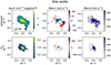 |
Fig. A.1. Total profiles [O III] (top) and Hα (bottom) flux, moment-1 and moment-2 maps. A S/N cut of 4 has been applied to generate the maps. The disc and biconical outflow components identified in Figs. 8 and 9, respectively, are here less evident. Hα is less affected by the outflow, and its moment-1 still reveal a NW-SE gradient likely associated with a disc rotation. |
Appendix B: Spatially integrated spectra of off-nuclear approaching and receding gas
Optical emission line properties from the NIRSpec integrated spectrum of NW cone (blueshifted outflow).
Optical emission line properties from the NIRSpec integrated spectrum of SW cone (redshifted outflow).
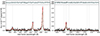 |
Fig. B.1. NIRSpec integrated spectrum of NE cone, showing the blueshifted outflow. The black curve identifies the integrated spectrum, integrated over a circular region identified by the light-blue crescent moon in the inset in Fig. 10; the total, multi-component best fit curve is in red, while the green and and grey Gaussian components show the systemic and outflow, respectively. The fit residuals are reported in the top panels. The most prominent emission lines are marked with grey vertical lines. |
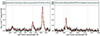 |
Fig. B.2. NIRSpec integrated spectrum of SW cone, showing the redshifted outflow. The black curve identifies the integrated spectrum, integrated over a circular region identified by the light-red crescent moon in the inset in Fig. 10; the total, multi-component best fit curve is in red, while the green and and grey Gaussian components show the systemic and outflow, respectively. The fit residuals are reported in the top panels. The most prominent emission lines are marked with grey vertical lines. |
All Tables
Properties of GS133 inferred from the optical emission lines of the NIRSpec integrated spectrum, obtained for the systemic (‘sys’), outflow (‘out’), and total (‘tot’) line profiles.
Optical emission line properties from the NIRSpec integrated spectrum of NW cone (blueshifted outflow).
Optical emission line properties from the NIRSpec integrated spectrum of SW cone (redshifted outflow).
All Figures
|
Fig. 1. Integrated spectrum of GS133. The blue curve identifies the VLT/VIMOS spectrum; the black line shows the JWST/NIRSpec spectrum, integrated over a circular aperture of r = 0.5″. The most prominent emission lines are marked with grey vertical lines. The gap in the middle of the NIRSpec spectrum (λrest ∼ 5400 Å) is due to the separation between the two NIRSpec detectors. |
| In the text | |
|
Fig. 2. JWST/NIRSpec integrated spectrum of GS133. The black curve identifies the integrated spectrum; the total, multi-component best-fit curve is in red, while all individual Gaussian components are shown with different colours. The fit residuals are reported in the top panels. The most prominent emission lines are marked with grey vertical lines. Light and dark yellow shaded areas in the right panel mark the [O III] emission within ±2000 km s−1 and ±1000 km s−1, respectively, from the GS133 systemic redshift. |
| In the text | |
|
Fig. 3. VLT/VIMOS spectrum with best-fit results. The flux is normalised to the continuum. The blue curve identifies the integrated spectrum; the total, multi-component best fit curve is in red, while all individual Gaussian (Voigt) components are shown in yellow (green). The most prominent line transitions are marked with grey vertical lines. |
| In the text | |
|
Fig. 4. VoigtFit models in velocity space. The normalised spectra, shown in blue with 3σ error bars, display the regions in the vicinity of the absorption lines; the best-fit models are overlaid in red. Carbon, nitrogen and silicon lines are fitted simultaneously, with two kinematic components; the vertical lines identify the velocity centroids for each kinematic component. For the doublets, the reported velocities are calculated with respect to the systemic of the blue line of the doublet; the kinematic components associated with the blue transitions are in orange, those of the red transitions are in purple. The narrow top panels show the best-fit residuals, with 3σ confidence intervals. Emission line contributions were removed prior to the VoigtFit modelling. |
| In the text | |
|
Fig. 5. GS133 spectrum showing tentative Balmer absorption detection in the vicinity of Hα and [N II] emission lines. The black curve shows the integrated spectrum in velocity space, with v = 0 km s−1 at the position of the Hα line. The red curve (with 1σ uncertainties in light-red) displays the residuals obtained by subtracting the best-fit Gaussian emission lines presented in Fig. 2. Two low S/N absorption features are detected close to the orange vertical lines, which mark the velocities of the mini-BAL features observed in the UV (see Table 2). |
| In the text | |
|
Fig. 6. [O III] velocity-channel maps (first-to-third panels) and spectroastrometry [O III] line positions (right panel). First to third panels: The velocity-channel maps were extracted from the ranges labelled in the individual panels. For each flux distribution, we report 3 and 5σ contour levels. The black cross identifies the GS133 nucleus, as inferred from spectroastrometry position of spectrally integrated [O III] profile (i.e. considering all velocity channels together); the white ellipse in the third panel represents the NIRSpec point spread function (PSF) at ∼2.2 μm (the [O III] observed wavelength) estimated by D’Eugenio et al. (2024); a scale bar and a compass are also reported in the first map. Right panel: Spectroastrometry of the [O III] emission, i.e. centroid positions of the line in the different velocity channels, covering a relatively small portion of the spatial extent shown in the velocity-channel maps (see white box in the third panel). The points are colour-coded by the channel velocity. The dot-dashed line roughly identifies the outflow axis, while the dotted line shows the tentative kinematic major axis of the GS133 rotating disc. |
| In the text | |
|
Fig. 7. Velocity diagram for the individual Gaussian components used to model the emission line profiles in the GS133 datacube. The measurements are coloured by the distance from the AGN. The blue lines isolate the Gaussian components with FWHM < 400 km s−1 and |Δv|< 120 km s−1 used to separate the narrow emission line kinematics (reported in Fig. 8) from the outflow kinematics (Fig. 9). |
| In the text | |
|
Fig. 8. [O III] (top) and Hα (bottom) flux, moment-1 and moment-2 maps for the systemic kinematic component. A S/N cut of 4 has been applied to generate the maps. The moment-1 maps of both lines show evidence of rotating gas in the QSO host, but neither moment-2 map shows a peak at the nuclear position (identified by a black cross). |
| In the text | |
|
Fig. 9. [O III] (top) and Hα (bottom) flux, moment-1 and moment-2 maps for the outflow kinematic component. A S/N cut of 4 has been applied to generate the maps. The [O III] maps show a typical biconical outflow structure, oriented along the NE-SW direction, consistent with our spectro-astrometry analysis (Sect. 4.1). The Hα flux distribution is less extended, as this Balmer line is fainter than [O III]. |
| In the text | |
|
Fig. 10. Standard BPT diagnostic diagram. The colour-coded squares show GS133 single-spaxel measurements associated with the spatial regions shown in the top-right panel; green-to-blue colours mark increasing line ratios, as indicated with the arrow in the bottom-left part of the diagram; only spaxels with S/N > 3 in all lines are shown. The large green and purple circles display the line ratios measured from r = 0.5″ spatially integrated regions, for the systemic and outflow components, as labelled: the large crescent moon symbols refer to the outflow component line ratios measured in circular regions marked in the inset (with the same crescent moon symbols). The solid (Kewley et al. 2001) and dashed (Kauffmann et al. 2003) curves commonly used to separate purely star-forming galaxies (below the curves) from AGN (above the curves) are also reported. Finally, the BPT shows local galaxies from SDSS (Abazajian et al. 2009, indicated in grey), and additional measurements for z = 2.6 − 6.7 sources from the literature: star-forming galaxies are marked with small green symbols and refer to CEERS (Calabrò et al. 2023) and JADES (Scholtz et al. 2023) surveys, while AGN are marked with small orange symbols and refer to JADES (Scholtz et al. 2023) and GA-NIFS (Perna et al. 2023b) surveys. |
| In the text | |
|
Fig. 11. Hydrogen densities and column densities predicted by CLOUDY photoionisation models for the two mini-BAL components. Only models with χ2 < 5 are shown and the sizes of the symbols are inversely scaled with χ2. In addition, models are colour coded according to their ionisation parameters. Both outflow components have low-density and high-density solutions, although the high-density solution would imply extremely thin layers of gas. |
| In the text | |
|
Fig. 12. MOKA3D model (left) and moment maps from NIRSpec data and MOKA3D model (right panels). In the 3D representations of the GS133 outflow structure, the XY represents the plane of the sky, while Z axis is the LOS. The observer is positioned on the left, and sees as blueshifted (redshifted) all the approaching (receding) gas, according to the colour bar; largest bubbles identify brightest clumps. The three-by-three panels show the comparison between the flux, Mom-1 and Mom-2 maps of [O III] (top panels) and MOKA3D model (middle panels) for the GS133 bi-conical outflow. The bottom panels present the residuals obtained subtracting the model from the data. |
| In the text | |
|
Fig. 13. JWST/NIRCam F115W/F200W/F444W cutout showing the close environment of GS133. The red dashed box marks the NIRSpec IFS FOV, while the white contours show the Chandra 0.5–7 keV emission from Luo et al. (2017), highlighting the position of two X-ray AGN with a projected separation of ∼130 kpc and a velocity offset of ∼5000 km s−1 (Δz = 0.08). The apparent offset between the NIR and X-ray positions can be attributed to Chandra’s low angular resolution and the fact that the Chandra image is composed of multiple observations taken with varying aim points and roll angles. The inset shows a zoom-in on GS133. The images are oriented north up, east left. |
| In the text | |
|
Fig. A.1. Total profiles [O III] (top) and Hα (bottom) flux, moment-1 and moment-2 maps. A S/N cut of 4 has been applied to generate the maps. The disc and biconical outflow components identified in Figs. 8 and 9, respectively, are here less evident. Hα is less affected by the outflow, and its moment-1 still reveal a NW-SE gradient likely associated with a disc rotation. |
| In the text | |
|
Fig. B.1. NIRSpec integrated spectrum of NE cone, showing the blueshifted outflow. The black curve identifies the integrated spectrum, integrated over a circular region identified by the light-blue crescent moon in the inset in Fig. 10; the total, multi-component best fit curve is in red, while the green and and grey Gaussian components show the systemic and outflow, respectively. The fit residuals are reported in the top panels. The most prominent emission lines are marked with grey vertical lines. |
| In the text | |
|
Fig. B.2. NIRSpec integrated spectrum of SW cone, showing the redshifted outflow. The black curve identifies the integrated spectrum, integrated over a circular region identified by the light-red crescent moon in the inset in Fig. 10; the total, multi-component best fit curve is in red, while the green and and grey Gaussian components show the systemic and outflow, respectively. The fit residuals are reported in the top panels. The most prominent emission lines are marked with grey vertical lines. |
| In the text | |
Current usage metrics show cumulative count of Article Views (full-text article views including HTML views, PDF and ePub downloads, according to the available data) and Abstracts Views on Vision4Press platform.
Data correspond to usage on the plateform after 2015. The current usage metrics is available 48-96 hours after online publication and is updated daily on week days.
Initial download of the metrics may take a while.