| Issue |
A&A
Volume 696, April 2025
|
|
|---|---|---|
| Article Number | A59 | |
| Number of page(s) | 25 | |
| Section | Extragalactic astronomy | |
| DOI | https://doi.org/10.1051/0004-6361/202453430 | |
| Published online | 04 April 2025 | |
GA-NIFS: High number of dual active galactic nuclei at z ∼ 3
1
Centro de Astrobiología (CAB), CSIC–INTA, Cra. de Ajalvir Km. 4, 28850 Torrejón de Ardoz, Madrid, Spain
2
Università di Firenze, Dipartimento di Fisica e Astronomia, Via G. Sansone 1, 50019 Sesto F.no, Firenze, Italy
3
INAF – Osservatorio Astrofisico di Arcetri, Largo E. Fermi 5, I-50125 Firenze, Italy
4
Kavli Institute for Cosmology, University of Cambridge, Madingley Road, Cambridge CB3 0HA, UK
5
Cavendish Laboratory – Astrophysics Group, University of Cambridge, 19 JJ Thomson Avenue, Cambridge CB3 0HE, UK
6
Max-Planck-Institut für Extraterrestrische Physik (MPE), Gießenbachstraße 1, 85748 Garching, Germany
7
Institut d’Astrophysique de Paris, UPMC et CNRS, UMR 7095, 98 Bis bd Arago, F-75014 Paris, France
8
Department of Physics and Astronomy, University College London, Gower Street, London WC1E 6BT, UK
9
Department of Physics, University of Oxford, Denys Wilkinson Building, Keble Road, Oxford OX1 3RH, UK
10
Sorbonne Université, CNRS, UMR 7095, Institut d’Astrophysique de Paris, 98 Bis bd Arago, 75014 Paris, France
11
Scuola Normale Superiore, Piazza dei Cavalieri 7, I-56126 Pisa, Italy
12
European Southern Observatory, Karl-Schwarzschild-Strasse 2, 85748 Garching, Germany
13
European Space Agency, c/o STScI, 3700 San Martin Drive, Baltimore, MD 21218, USA
14
European Space Agency, ESAC, Villanueva de la Cañada, E-28692 Madrid, Spain
15
NRC Herzberg, 5071 West Saanich Rd, Victoria, BC V9E 2E7, Canada
16
Los Alamos National Laboratory, Los Alamos, NM 87545, USA
⋆ Corresponding author; This email address is being protected from spambots. You need JavaScript enabled to view it.
Received:
13
December
2024
Accepted:
13
February
2025
Abstract
Context. Merger events can trigger gas accretion onto supermassive black holes (SMBHs) located at the centre of galaxies and form close pairs of active galactic nuclei (AGNs). The fraction of AGNs in pairs offers critical insights into the dynamics of galaxy interactions, SMBH growth, and their co-evolution with host galaxies. However, the identification of dual AGNs is difficult, as it requires high-quality spatial and spectral data; hence, very few pairs have been found in the distant Universe so far.
Aims. This study is aimed at providing a first observational estimate of the fraction of dual AGNs at 2 < z < 6 by analysing a sample of 16 AGNs observed with the JWST Near-InfraRed Spectrograph (NIRSpec) in integral field mode, as part of the GA-NIFS survey. For two AGNs in our sample, we also incorporated archival VLT/MUSE data to expand the search area.
Methods. We searched for nearby companion galaxies and emission-line sources within the ∼20 × 20 kpc field of view of the NIRSpec data cubes, extending up to ∼50 kpc using the MUSE data cubes. We analysed the spectra of such emitters to determine their physical and kinematic properties.
Results. We report the serendipitous discovery of a triple AGN system and four dual AGNs (two of which had been considered as candidates), with projected separations in the range 3−28 kpc. The results of this study more than double the number of known multiple AGNs at z > 3 at these separations. Their AGN classification is mainly based on standard optical emission line flux ratios, as observed with JWST/NIRSpec, and complemented with additional multi-wavelength diagnostics. The identification of these 3−5 multiple AGNs out of the 16 AGN systems in the GA-NIFS survey (i.e. ∼20−30%) suggests they might be more common than previously thought from other observational campaigns. Moreover, our inferred fraction of dual AGN moderately exceeds predictions from cosmological simulations that mimic our observational criteria (∼10%).
Conclusions. This work highlights the exceptional capabilities of NIRSpec for detecting distant dual AGNs, prompting new investigations to constrain their fraction across cosmic time.
Key words: galaxies: active / galaxies: high-redshift / quasars: supermassive black holes
© The Authors 2025
 Open Access article, published by EDP Sciences, under the terms of the Creative Commons Attribution License (https://creativecommons.org/licenses/by/4.0), which permits unrestricted use, distribution, and reproduction in any medium, provided the original work is properly cited.
This article is published in open access under the Subscribe to Open model. This email address is being protected from spambots. You need JavaScript enabled to view it. to support open access publication.
1. Introduction
Since supermassive black holes (SMBHs) are believed to be present at the centre of most massive galaxies (e.g. Magorrian et al. 1998), merging systems with two or more SMBHs are a natural and expected occurrence (e.g. Koss et al. 2012, 2023). Studies of these objects have been receiving increasing attention, as they can be used to constrain the link between galaxy mergers and SMBH feeding and feedback effects across cosmic time, which is a key ingredient for galaxy evolution models (De Rosa et al. 2019; Volonteri et al. 2022; Chen et al. 2023). Moreover, these SMBH pairs are the parent population of the systems that will eventually merge, producing the gravitational wave signals now detected by the pulsar timing array (PTA) experiments (e.g. EPTA Collaboration et al. 2023; Agazie et al. 2023a) for SMBHs with masses in the range 108 − 109 M⊙. Similarly, mergers involving lighter SMBHs (104 − 107 M⊙) are expected to be detectable with the upcoming Laser Interferometric Space Antenna (LISA; e.g. Agazie et al. 2023b). However, beyond the local Universe (e.g. Voggel et al. 2022), systems with multiple SMBHs can only be detected when both nuclei shine as active galactic nuclei (AGNs) simultaneously. This phenomenon occurs during brief active phases within the much longer galaxy merging process (e.g. Capelo et al. 2017).
Cosmological simulations predict a fraction of AGN pairs, separated by hundreds to few thousands parsecs, out of the total number of AGNs, of the order of a few percent in the redshift range 1 < z < 5, depending on the selection criteria on luminosity, distance, and mass of the selected systems (e.g. De Rosa et al. 2019; Volonteri et al. 2022; Chen et al. 2023; Puerto-Sánchez et al. 2025). Observations have been consistent to date with these theoretical predictions; so far, only very few dual AGNs have been found at z > 1 (e.g. Lemon et al. 2023; Mannucci et al. 2022, 2023).
The detection of dual AGNs is hampered by several challenges. The spatial resolution and sensitivity constraints often preclude resolving small separations, especially in distant galaxies. Moreover, the distinction between dual AGNs and other phenomena, such as gravitational lensing effects, requires high-quality spectral and spatial data, often requiring dedicated follow-up observations. Many dual AGNs have been discovered serendipitously (e.g. Shields et al. 2012; Husemann et al. 2018; Izumi et al. 2024) thanks to these limitations (De Rosa et al. 2019). However, more recently, systematic searches have been initiated thanks to the development of new techniques taking full advantage of the all-sky Gaia database (Gaia Collaboration 2018). The Gaia-Multi-Peak (GMP, Mannucci et al. 2022) technique facilitates the identification of dual AGN candidates at separations in the range of 0.1−0.7″ (e.g. 0.8−5.5 kpc at z = 3), searching for multiple peaks in the light profile of the Gaia sources. Another method is the Varstrometry technique (e.g. Hwang et al. 2020), which extends systematic searches for dual AGN candidates down to even lower separations by exploiting the temporal displacements of the photocentre of variable, unresolved sources. These new methods have been shown to be effective in discovering new dual AGN candidates (up to z ∼ 3; Mannucci et al. 2023; Lemon et al. 2023). However, they are generally limited to the relatively bright targets detected by Gaia, requiring the two AGN components to have comparable luminosities, and needing dedicated spectroscopic follow-up strategies to spatially resolve the candidate AGN pairs. Moreover, spectroscopic observations are required to distinguish multiple spatial components due to gravitational lensing of a single active galaxy from real AGN pairs (Lemon et al. 2023; Scialpi et al. 2024). These methods also have an important observational bias, as they require these systems to have significant emission in the optical band (∼4000 − 9500 Å) to be selected with Gaia. As a consequence, all dual AGNs discovered with Gaia are unlikely to be heavily affected by dust extinction. This is an important limitation, since an enhanced level of AGN obscuration is actually expected in late-stage mergers (e.g. Hopkins et al. 2016; Ricci et al. 2017; Perna et al. 2018; Koss et al. 2018). Therefore, the dual AGNs confirmed so far only provide a lower limit to their actual prevalence, especially at high redshifts (e.g. Li et al. 2024).
With its orders of magnitude improvement in sensitivity and resolution across the wavelength range from 0.6 to 29 μm compared to the previous generation of infrared telescopes (Rigby et al. 2023), JWST reveals our Universe in a whole new light. Specifically, it is opening the opportunity to study in detail the environment of AGNs in the early Universe by probing their emission in the rest-frame ultraviolet (UV) and optical spectral ranges. The first JWST spatially resolved spectroscopic observations, for instance obtained with the integral field spectrograph (IFS) of NIRSpec (Jakobsen et al. 2022; Böker et al. 2022) and the wide-field slitless spectroscopy (WFSS) mode of NIRCam (Greene et al. 2017) have already revealed that high-z AGNs are often surrounded by close companions (Kashino et al. 2022; Wylezalek et al. 2022; Yang et al. 2023; Perna et al. 2023; Marshall et al. 2023, 2024; Übler et al. 2023, 2024a; Schindler et al. 2024). Moreover, JWST observations show tidal bridges and tails at kiloparsec scales connecting the AGN with the companions, thereby revealing the presence of gravitational interactions up to z ∼ 7 (e.g. Marshall et al. 2023; Loiacono et al. 2024). These spectroscopic data also help unveil the nature of the AGN companions; for instance, classical emission line flux ratio diagnostics such as the optical and UV diagrams (e.g. Baldwin et al. 1981; Feltre et al. 2016; Nakajima & Maiolino 2022) can be used to identify multiple AGNs (e.g. Perna et al. 2023; Zamora et al. 2024).
In this work, we report the discovery of an AGN triplet, along with two secure and two candidate dual AGNs at z ∼ 3. They have projected separations between 3 and 28 kpc and are located in the GOODS-S (Giavalisco et al. 2004) and COSMOS fields (Scoville et al. 2007). Importantly, this work doubles the number of known multiple AGN systems at z ≳ 3 with separations < 30 kpc (Mannucci et al. 2023). All AGN pairs have been observed with NIRSpec IFS; the triple AGN has been instead identified by combining NIRSpec and archival observations from the optical IFS Multi Unit Spectroscopic Explorer (MUSE) at the Very Large Telescope (VLT). The sample of multiple AGN systems was drawn from a larger sample of 16 AGN systems at 2 < z < 6, targeted as part of the JWST programme “Galaxy Assembly with NIRSpec IFS” (GA-NIFS1). Some of these 16 targets have been already presented in the literature by our team and they appear in Parlanti et al. (2024, the target GS539, also know as Aless073.1), Übler et al. (2023, GS3073), Pérez-González et al. (2024, Jekyll & Hyde), D’Eugenio et al. (2024, GS10578), and Perna et al. (2025, GS133).
The paper is outlined as follows. Section 2 introduces the GA-NIFS survey and the sample of AGNs analysed in this work. In Sect. 3 we describe our JWST/NIRSpec IFS observations and data reduction procedures, as well as the archival data used to complement our analysis. The detailed data analysis of spectroscopic data is reported in Sect. 4. The optical spectra of our dual AGNs and emission line diagnostics employed for their classification are presented in Sect. 5.1. The UV spectra and diagnostics used to classify the third active nucleus in one of our systems are detailed in Sect. 5.2. The AGN and host galaxy properties of these systems are examined in Sect. 5.3–5.6. Finally, we discuss our results and present our estimate of the dual AGN fraction in Sect. 6. We conclude with a summary of our findings in Sect. 7. Throughout, we adopt a Chabrier (2003) initial mass function (0.1 − 100 M⊙) and a flat ΛCDM cosmology with H0 = 70 km s−1 Mpc−1, ΩΛ = 0.7, and Ωm = 0.3. In our analysis of NIRSpec data, we use vacuum wavelengths according to their calibration. Similarly, for MUSE data, we use vacuum wavelengths, consistent with the standard pre-JWST practice.
2. GA-NIFS sample of AGNs at 2 < z < 6
GA-NIFS is a JWST Guaranteed Time Observations (GTO) programme aimed at characterising the internal structure and close environment of a sample of z > 2 galaxies, as well as to investigate the physical processes driving galaxy evolution across cosmic time. It plans to observe 55 targets with NIRSpec IFS in JWST cycles 1 and 3, including both star-forming galaxies (SFGs) and AGNs (e.g. Jones et al. 2024; Arribas et al. 2024; Parlanti et al. 2025; Rodríguez Del Pino et al. 2024; Übler et al. 2024b).
The GA-NIFS sub-sample of non-active galaxies were heterogeneously selected among the most luminous and/or extended sources (as observed in Lyα, NIR, and/or mm wavelengths), together with a few well studied sources (e.g. Jekyll & Hyde; Schreiber et al. 2018; Pérez-González et al. 2024) to increase the leverage of IFS capabilities.
The sub-sample of active galaxies includes sources at z < 6 residing in the COSMOS and GOODS-S fields and selected solely for their X-ray emission L2 − 10 keV ≳ 1044 erg s−1 (from Marchesi et al. 2016; Luo et al. 2017), which is unambiguously attributed to AGN emission. This sub-sample consists of 7 sources in GOODS-S and 6 in COSMOS. A careful inspection of the NIRSpec data of other GA-NIFS targets in the same cosmological fields – but not fitting in the above X-ray selection criterion – allowed us to identify additional targets hosting AGN: we unveiled the presence of AGN activity, based on BPT diagnostics (Baldwin et al. 1981), in two sources originally selected as non-active galaxies, GS19293 (Venturi et al., in prep.), and in the close surroundings of Jekyll (Pérez-González et al. 2024). GS3073 must also be considered an AGN, due to the detection of broad line region (BLR) emission in its rest-frame optical spectrum (Übler et al. 2023).
We note that the GA-NIFS survey also includes additional AGNs that have not been considered in this study. They were specifically selected due to their dense environments: LBQS 0302−0019 at z ∼ 3.3, with its own secondary obscured AGNs, presented in Perna et al. (2023); BR1202−0725 at z ∼ 4.7, also featuring a secondary AGN identified through NIRSpec IFS data, presented in Zamora et al. (2024). Since they reside in well-known overdensities, these two systems were excluded from this work, as their inclusion would bias our search of dual AGNs. We also excluded GS5001, a source we presented in Lamperti et al. (2024). Although GS5001 is detected in X-rays, it remains uncertain whether it hosts an AGN (see also Lyu et al. 2024). Additionally, since GS5001 is situated in a well-known overdense region, it was excluded from this work to maintain consistency in our sample selection. Similarly, we excluded the GN20 source we presented in Übler et al. (2024b), which also resides in an overdensity (e.g. Daddi et al. 2009; Crespo Gómez et al. 2024).
Additional targets at z > 6 from GA-NIFS (e.g. Christensen et al. 2023; Marshall et al. 2023) were not taken into account in this work because in these high-z sources the [N II] λ6583 is very faint and usually undetected. This is likely due to their lower metallicity (e.g. Kocevski et al. 2023; Übler et al. 2023; Maiolino et al. 2024a; Ji et al. 2024), or because the line is redshifted out of the spectral range of NIRSpec (e.g. Marshall et al. 2024); hence, it precludes the use of BPT diagnostics to discover AGN emission in their companion sources. Other diagnostics might be required for these systems (e.g. the detection of faint [O III] λ4363, He IIλ4686 and BLR lines in the optical spectra; see e.g. Nakajima & Maiolino 2022; Tozzi et al. 2023; Übler et al. 2024a; Mazzolari et al. 2024) and we therefore defer this analysis to a forthcoming paper.
Therefore, the AGN sample studied in this paper consists of 16 systems at 2.0 < z < 5.6, with bolometric luminosities in the range Lbol = 1045 − 1047 erg s−1 (Circosta et al., in prep.). The complete list of targets is presented in Table A.1. The [O III] λ5007 emission line maps for the entire sample are presented in Fig. 1 and discussed in the next sections.
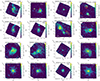 |
Fig. 1. [O III] and Hα maps of the close environments of GA-NIFS AGN systems. They trace the emitting gas observed with NIRSpec IFS in the velocity channels v ∈ [ − 100, 100] km s−1 with respect to the AGN systemic redshift. Contours represent regions where the line emission reaches a significance level of 5σ. Each contour corresponds to emission from a specific velocity bin of 200 km s−1, spanning the full velocity range from −1100 to +1100 km s−1. Cyan contours indicate blueshifted gas, while orange contours mark redshifted gas. Cross symbols identify the AGN position in more complex (interacting) systems. All but GS3073 maps were obtained from NIRSpec cubes with 0.05″/pixel; for GS3073 we opted for the use of the finest 0.03″/pixel sampling to show the disturbed morphology due to very nearby companions (see also Fig. A.1 in Ji et al. 2024). All images are oriented north up, with east to the left. |
3. Observations and data reduction
3.1. NIRSpec IFS data
The targets presented in this work were observed as part of the NIRSpec IFS GTO survey GA-NIFS (e.g. Perna 2023), under programmes #1216 (PI: Kate Isaak) and #1217 (PI: Nora Luetzgendorf). Information on the NIRSpec observations is reported in Table A.1.
The observational design was chosen in order to cover all main optical lines from Hβ to [S II]λλ6716, 31 doublet lines with a high spectral resolution (R ∼ 2700) at z = 3 − 6. Therefore, for all but two targets, we used the grating-filter pair G235H/F170LP. The source GS3073, at z = 5.55, was observed with G395H/F290LP; then, GS539, at z = 4.76, was observed with both G235H/F170LP and G395H/F290LP configurations. Next, COS2949 was observed with G235H/F170LP; we note that it was included in the GA-NIFS survey because it is listed as a z = 3.571 AGN with a spectroscopic redshift classified as ‘secure’ in the COSMOS catalogues. However, NIRSpec observations have revealed that COS2949 is at z = 2.0478. For this reason, the NIRSpec wavelength range only covers the Hα complex on its bluest side, missing the [O III] and Hβ emission lines.
Exposure times range from ≲1 hour for X-ray-selected AGNs, to ∼4 − 5 hours for the sources originally selected as (fainter) star-forming systems. Therefore, the quality of the data in our sample is not homogeneous. However, all targets have well detected emission lines, and display plenty of faint companions in the NIRSpec field of views (FOVs).
Raw data files were downloaded from the MAST archive and subsequently processed with the JWST Science Calibration pipeline version 1.8.2 under CRDS context jwst_1068.pmap. We made several modifications to the default three-stages reduction to increase data quality, which are described in detail by Perna et al. (2023) and briefly reported here. We patched the pipeline to avoid over-subtraction of elongated cosmic ray artefacts during the Stage1. The individual count-rate frames were further processed at the end of the pipeline Stage1, to correct for different zero-level in the individual (dither) frames, and subtract the vertical 1/f noise. In addition, we made the following corrections to the *cal.fits files after Stage 2: we masked pixels at the edge of the slices (two pixels wide) to conservatively exclude pixels with unreliable sflat corrections; we removed regions affected by leakage from failed open shutters; finally, we used a modified version of LACOSMIC (van Dokkum 2001) to reject strong outliers before the construction of the final data cube (D’Eugenio et al. 2024). The final cubes were combined using the drizzle method with pixel scales of 0.05″ and 0.03″, for which we used an official patch to correct a known bug. The smaller pixel scale is required to better characterise the closest dual AGNs, fully exploiting the spatial resolution of the data (D’Eugenio et al. 2024). The astrometric alignment of the NIRSpec data was computed relative to HST images that have been registered to Gaia DR3.
3.2. MUSE data
Two of the 16 systems in the GA-NIFS AGN sub-sample have archival VLT/MUSE data, from the MUSE-WIDE (Urrutia et al. 2019) and the MUSE-UDF (Bacon et al. 2017) surveys. These observations cover the rest-frame UV spectra of GS551 and GS10578, respectively.
Reduced MUSE datacubes were downloaded from the MUSE-WIDE cut-out service2, for the source GS551, and from the ESO archive, for GS10578. Their observational log is reported in Table A.1. Because the MUSE spectrograph does not operate in vacuum and the wavelength calibration is in standard air3 (Weilbacher et al. 2020), we converted them to vacuum before the fit analysis, consistent with NIRSpec. As for the NIRSpec observations, the astrometric alignment of the MUSE data was computed relative to HST images registered to Gaia DR3.
3.3. X-ray data
X-ray data offer complementary information for assessing AGN activity and constraining the physical properties of these systems. The X-ray properties of the sample, especially their X-ray flux measurements, were obtained from the catalogues of the X-ray deep fields COSMOS-Legacy survey (Civano et al. 2016; Marchesi et al. 2016) and the CDFS (Liu et al. 2017) for COSMOS and GOODS-S targets, respectively. We further used the full mosaics of COSMOS-Legacy (Civano et al. 2016) and CDFS (Liu et al. 2017) to estimate the upper limit 0.3−7 keV flux of the systems that are undetected in the X-rays. Moreover, we used one of the single exposures of the COSMOS-Legacy survey to study the X-ray morphology of COS1638 (obsID 15253, corresponding to the one in which our target is observed in the best conditions). We downloaded the raw data from the Chandra archive and reduced them with CIAO v4.15 (Fruscione et al. 2006) through the chandra_repro tool. The morphological analysis of COS1638 is presented in Sect. 5.6.
3.4. VIMOS data
In this work, we also analysed the rest-frame UV spectra of 5 X-ray detected, type 2 AGNs at z ∼ 3, observed as part of the survey “VANDELS: a VIMOS survey of the CDFS and UDS fields” (McLure et al. 2018) and previously identified by Saxena et al. (2020) and Mascia et al. (2023). They were observed using the MR grism and the GG475 filter, with a 1″ slit width and a slit length of 10″ oriented east-west on the sky. The total exposure time was ≈40 hours per target. This setup provides a wavelength coverage of 4800−10 000 Å with a nominal resolution of R = 580, corresponding to a velocity resolution of approximately 500 km s−1. The spectroscopic analysis presented in this work takes advantage of the VANDELS DR4 fully reduced spectra (Garilli et al. 2021), downloaded from the ESO archive4.
One of these VANDELS AGN, GS133, was also analysed as part of our GA-NIFS survey, with its UV spectrum thoroughly analysed in Perna et al. (2025). The five VANDELS targets (discussed in Sect. 6.2) enhance our investigation by contributing to the assessment of the reliability of UV diagnostic diagrams for identifying AGNs at high redshifts.
4. Data analysis
4.1. Identification of line emitters in NIRSpec data
To search for potential companion galaxies and line emitters near our AGN systems observed with JWST, we performed a spectral scan around the [O III]λ5007 and Hα emission lines. Specifically, we explored a velocity range from ∼ − 1000 to +1000 km s−1 relative to the systemic velocity of the AGN. The [O III] line is generally preferred due to its relative brightness compared to other optical lines, which aids in the clear identification of nearby emitters. However, in heavily obscured AGNs where [O III] is faint (e.g. GS539; Parlanti et al. 2024), Hα was used as an alternative. For COS2949, Hα was analysed instead of [O III] due to limited wavelength coverage.
Figure 1 shows emission line cutouts for each target, obtained integrating over the range v ∈ [ − 100, +100] km s−1, with contours tracing the 5σ-emission in 200 km s−1-wide bins at lower and higher velocities (up to ±1100 km s−1). Many of our 16 AGNs are situated in complex environments, showing signs of gravitational interactions (e.g. COS590, COS2949, COS1638), and several [O III] emitters within a few hundred km s−1 of the central AGN. In particular, close emitters are identified in 9 systems: COS590, COS1638, COS1656, COS2949, GS551, GS3073 (see also Übler et al. 2023), GS20936, Jekyll (Pérez-González et al. 2024), and GS10578 (D’Eugenio et al. 2024). A bright M star is identified in the vicinity of COS1118 (in the upper part of the NIRSpec FOV, at RA = 09:59:31, Dec = 02:13:34.3).
4.2. NIRSpec spectroscopic analysis
To investigate the nature of the line emitters in the vicinity of our GA-NIFS AGN, we extracted integrated spectra from circular apertures with r = 0.1″ centred at the peak position of all identified emitters (comprising the bright AGN), hence from regions broadly corresponding to the spatial resolution element of NIRSpec IFS observations (D’Eugenio et al. 2024).
We modelled their integrated spectra with a combination of Gaussian profiles. We fitted the most prominent gas emission lines by using the Levenberg-Marquardt least-squares fitting code CAP-MPFIT (Cappellari 2017). In particular, we modelled the Hα and Hβ lines, the [O III] λλ4959, 5007, [N II] λλ6548, 83, and [S II] λλ6716, 31 doublets applying a simultaneous fitting procedure (Perna et al. 2023), so that all line features corresponding to a given kinematic component have the same velocity centroid and full width at half maximum (FWHM). During the fit, we removed all Gaussian components, whose amplitude is characterised by a signal-to-noise ratio of S/N < 2. The modelling of the Hα and Hβ BLR emission in type 1 AGN sources required the use of broken power-law components (e.g. Cresci et al. 2015): they are preferred to a combination of extremely broad Gaussian profiles, because the former tend to minimise the degeneracy between narrow line region (NLR) and BLR emission. Finally, we used the theoretical model templates of Kovacevic et al. (2010) to reproduce the Fe II emission in the wavelength region 4000 − 5500 Å (see Perna et al. 2017a for details). The final number of kinematic components used to model the spectra is derived on the basis of the Bayesian information criterion (BIC, Schwarz 1978). The continuum emission, when detected, is modelled with a low-order polynomial function, and subtracted prior to fitting the emission lines. For GS10578, which shows strong stellar continuum and absorption line features, we used the model obtained by D’Eugenio et al. (2024).
Following Übler et al. (2023), the noise level was obtained from the ERR extension of the NIRSpec data cubes, after re-scaling it with a measurement of the standard deviation in the integrated spectrum in regions free of line emission to take into account correlations due to the non-negligible size of the PSF relative to the spaxel. The uncertainties in the emission line properties reported in this work were measured using Monte Carlo simulations (following e.g. Perna et al. 2015). We collected 50 mock spectra using the best-fit final models, added random noise, and fit them. The errors were then calculated by taking the range that contains 68.3% of values evaluated from the obtained distributions for each measurement.
4.3. Identification of line emitters in MUSE data
We used MUSE data cubes to identify possible companions and line emitters in the vicinity of GS10578 and GS551. This analysis followed the methodology previously applied to NIRSpec data but extended the search to a larger area beyond the relatively small NIRSpec FOV (∼3″ × 3″). Specifically, we conducted a spectral scan around the Lyα emission line, the brightest line in the UV regime; we covered a velocity range from −1400 to +1400 km s−1 relative to the AGN systemic velocity, with 400 km s−1 bins. The broader velocity range and larger binning reflect the lower S/N in the MUSE data cubes.
Figure 2 shows the emission line cutouts for both targets, obtained integrating over the range v ∈ [ − 200, 200] km s−1, with contours tracing the 4σ-emission in bins at v < −200 km s−1 and v > 200 km s−1. They show extended nebulae surrounding the central X-ray detected AGNs. Moveover, GS10578 shows two close Lyα emitters, brighter than the one of the central AGN. GS551 shows a faint Lyα emitter at 20 kpc towards the south-east, and diffuse emission towards the north and north-west.
4.4. Spectral fit of MUSE data
The MUSE spectroscopic data were analysed following the same general procedures described in the previous section. In particular, we extracted the spectra of individual emitters by integrating regions optimised to increase the S/N for each source. The fit analysis required the use of a single Gaussian profile for the lines He IIλ1640, C IVλλ1549, 1550, and C III] λ1907, 1909 (with the latter two modelled taking into account their doublet nature), which are the lines required for the classification of AGNs and SFGs according to the UV diagnostics proposed by Feltre et al. (2016) and Nakajima & Maiolino (2022). Also for these targets, the outcomes of the spectroscopic analysis are discussed in the following sections.
Dual (and triple) AGNs.
5. Results
Figure 1 illustrates that nine out of the 16 GA-NIFS targets at z = 2 − 6 have close [O III] and Hα line emitters within a ∼20 × 20 kpc2 area surrounding the main source. Similarly, Fig. 2 demonstrates that both targets with available MUSE observations contain Lyα emitters at distances extending to several tens of kiloparsecs. In this section we examine five of these systems, which are those with newly identified companions that likely host accreting SMBHs. Their main properties are summarised in Table 1, and discussed in detail in Appendix B. For clarity, we refer to the brighter active galaxy in each system as the ‘primary’ AGN (AGN-A) and the fainter one as the ‘secondary’ AGN (AGN-B). Additionally, in one system, we identified a further line emitter classified as the ‘tertiary’ AGN, labelled AGN-C. These five systems also present fainter emitters in addition to those classified as AGNs. For simplicity, we refer to these sources as ‘clumps’; they may correspond to small satellite galaxies (e.g. near COS1656 and GS10578) or to star-forming regions in tidal tails or debris resulting from gravitational interactions between galaxies (e.g. near Jekyll), associated with faint continuum emission.
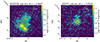 |
Fig. 2. Lyα maps of the close environments of GS10578 (left) and GS551 (right). They trace the emitting gas with v ∈ [ − 200, 200] km s−1 observed with MUSE. The cyan (orange) contours indicate the Lyα emission at 4σ in velocity bins of 400 km s−1, from −1400 to +1400 km s−1. The cross symbols identify the (NIRSpec) AGN positions. The coordinate grids highlight the different rotation of MUSE data with respect to the standard north-east up-left configuration. |
To assess the nature of each line emitter and determine whether their emission originates from AGN activity, star formation, or shock excitation, we employed a series of emission-line diagnostics. These diagnostics also allowed us to evaluate whether the observed line emission is due to external ionisation from the primary AGN or if it indicates an intrinsic ionising source, such as a secondary AGN within the companion galaxy. For COS1638, we also present tentative evidence of X-ray emission from the secondary AGN, analysing archival Chandra data. Finally, rest-frame optical and UV observations were complemented with available multi-wavelength information to constrain the stellar masses of the primary and secondary AGNs. The specific diagnostics used to characterise our targets are described in the following subsections. A detailed spatially resolved study of all GA-NIFS AGNs will be presented in forthcoming works (Bertola et al., in prep.; Venturi et al., in prep.).
5.1. Optical emission lines and BPT diagnostics
Figures 3, 4, 5, 6, and 7 show the NIRSpec spectra of the line emitters along with their best-fit models. For each system, we also provide a zoomed-in [O III] map to illustrate the spatial locations of these emitters. All maps were generated from data cubes with a 0.03″/pixel resolution, to fully leverage the angular resolution of NIRSpec. Optical spectra were extracted from cubes with a 0.05″/pixel scale for most targets, optimising the S/N. However, for the clump near GS10578, the clump and AGN-B close to COS1656 that overlap on the LOS, and the X-ray AGN GS551 and its close companion, we extracted the spectra from cubes with the finest sampling (0.03″/pixel) to minimise PSF contaminations.
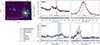 |
Fig. 3. [O III] map (top-left) and integrated spectra of the dual AGN system associated with COS1638. The [O III] map is obtained by integrating the [O III] emission over specific velocity ranges (as labelled), in order to highlight the primary (AGN-A) and secondary (AGN-B) nuclei, together with additional structures at the same redshift of the active galaxies. The panels on the right show the integrated spectra of the primary (top) and secondary (bottom) AGNs, extracted from the circular regions labelled in the map. The legend displays the individual Gaussian components and best-fit curves shown in the spectra; best-fit total profiles are represented in red for AGN-A and in blue for AGN-B. Residuals, defined as the difference between the observed data and the best-fit model, are displayed at the bottom of each panel; average ±3σ uncertainties on the data are also reported with horizontal grey shaded regions. The vertical blue and green shaded areas correspond to the velocity channels used to generate the [O III] map and contours in the top-left panel, respectively. Both targets present broad lines due to powerful outflows. |
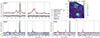 |
Fig. 4. [O III] map (top-right) and integrated spectra of the dual AGN system and a faint clump associated with COS1656. The [O III] map is obtained by integrating the [O III] emission over a velocity range from −200 to +200 km s−1, in order to highlight the primary (AGN-A) and secondary (AGN-B) nuclei; the contours trace the emission at v ∈ [ − 800, −600] associated with a clump close to AGN-B. The remaining panels show the integrated spectra of the primary (top-left) and secondary (bottom-left) AGNs, as well as of the clump (bottom-right), extracted from the circular regions labelled in the map. The legend display the individual Gaussian components and best-fit curves shown in the spectra; best-fit total profiles are represented in red for AGN-A, in blue for AGN-B, and in magenta for the clump. Residuals, defined as the difference between the observed data and the best-fit model, are displayed at the bottom of each panel; average ±3σ uncertainties on the data are also reported with grey shaded regions. The vertical green and blue shaded areas at ∼5007 Å mark the channels used to generate the [O III] map and contours in the top-right panel, respectively. |
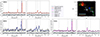 |
Fig. 5. [O III] map (top-right) and integrated spectra of the dual AGN system and a faint clump associated with Jekyll & Hyde. The [O III] map is obtained by integrating the line emission over specific velocity ranges (as labelled), in order to highlight the primary (Eastfield, AGN-A) and secondary (Mr West, AGN-B) nuclei, together with additional structures at the same redshift of the active galaxies. The remaining panels show the integrated spectra of the primary (top-left) and secondary (bottom-left) AGNs, as well as of a compact clump between the two brightest sources (bottom-right). The legend display the individual Gaussian components and best-fit curves shown in the spectra. Residuals, defined as the difference between the observed data and the best-fit model, are displayed at the bottom of each panel, with grey shaded regions indicating the average ±3σ uncertainties on the data. The vertical shaded areas at ∼5007 Å mark the channels used to generate the [O III] three-colour map. |
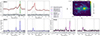 |
Fig. 6. [O III] map (top-right) and integrated spectra of the dual AGN system and a faint clump associated with GS10578. The [O III] map is obtained by integrating the [O III] emission over a velocity range from −200 to +200 km s−1, in order to highlight the primary (AGN-A) and secondary (AGN-B) nuclei, together with additional structures at the same redshift of the active galaxies. The remaining panels show the integrated spectra of the primary (top-left) and secondary (bottom-left) AGNs, as well as of a compact clump between the two brightest sources (bottom-right). The legend display the individual Gaussian components and best-fit curves shown in the spectra. Residuals, defined as the difference between the observed data and the best-fit model, are displayed at the bottom of each panel, with grey shaded regions indicating the average ±3σ uncertainties on the data. The vertical green shaded area at ∼5007 Å mark the channels used to generate the [O III] map. |
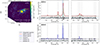 |
Fig. 7. [O III] map (top-right) and integrated spectra of the candidate dual AGN system associated with GS551. The [O III] map is obtained by integrating the [O III] emission over a specific velocity range (as labelled), in order to highlight the primary (AGN-A) and secondary (AGN-B) nuclei, together with additional structures at the same redshift of the active galaxies. The remaining panels show the integrated spectra of the primary (top-right) and secondary (bottom-right) AGNs. The legend display the individual Gaussian components and best-fit curves shown in the spectra; best-fit total profiles are represented in red for AGN-A, and in blue for AGN-B. Residuals, defined as the difference between the observed data and the best-fit model, are displayed at the bottom of each panel, with grey shaded regions indicating the average ±3σ uncertainties on the data. The vertical green shaded area at ∼5007 Å marks the channels used to generate the [O III] map, while the blue shaded area marks those associated with extended emission marked with contours overlapping the map. |
In all figures, the red colour is used to identify the primary AGN both in spectra (red best-fit curves) and maps (red circles). The secondary, fainter AGN is shown in blue. Any additional sources in the vicinity are marked in magenta for clarity. A detailed description of each system is reported in Appendix B. Here we report the main outcomes of the spectroscopic analysis in terms of emission-line ratios and the presence of strong outflows.
For at least one target, AGN-B in COS1638, the detection of a prominent [O III] outflow with velocities reaching several thousand km s−1 (Table A.2) serves as compelling evidence of AGN activity. Such extreme velocities are inconsistent with starburst-driven outflows (e.g. Cicone et al. 2016; Carniani et al. 2024) and are instead indicative of energetic AGN winds (e.g. Perrotta et al. 2019; Villar Martín et al. 2020; Tozzi et al. 2024). In particular, the [O III] features in COS1638-B are characteristic of AGN classified as ‘blue outliers’ (Zamanov et al. 2002), where the peak of [O III] is blueshifted relative to the systemic velocity corresponding to the peak of the Hα narrow component. Similar profiles are observed in the secondary AGN of the BR1202–0725 system, reported in Zamora et al. (2024).
Asymmetric emission line profiles are also observed in other AGN-B, albeit with less pronounced wings that could correspond to weaker outflows (Figs. 4, 5, 7). This emission might result from starburst or AGN winds but could also be due to gravitational interactions between the dual AGN hosts. Additionally, PSF smearing may contribute to the broadening of line profiles, as seen in AGN-B of GS551, and in AGN-B and the clump associated with COS1656. In fact, all newly discovered line emitters lie within 10 kpc from the central primary AGN, and have velocity shifts of a few hundreds of km s−1, indicating that gravitational interactions are probable. Filamentary structures likely associated with tidal tails are also detected in the close surroundings of COS1638 (Fig. 3), Jekyll (Fig. 5), and GS551 (Fig. 7). Consequently, except for COS1638 AGN-B, the kinematic signatures alone cannot be reliably used to confirm the presence of multiple AGNs within these systems. To asses the nature of the newly discovered line emitters, we used line ratio diagnostics.
The ionisation source of each AGN is determined using the standard BPT diagnostic diagram (Baldwin et al. 1981), shown in Fig. 8. In particular, we report all the line ratios with clear AGN ionisation (AGN-A in red, AGN-B in blue); hence, it does not show those of individual clumps whose line ratios could be associated both with star formation and AGNs, because they have upper limits in the [N II]/Hα. We also excluded from the BPT the primary AGN in COS1638, as it is affected by fit degeneracy between BLR and NLR components. For completeness, the individual line ratios of all line emitters in the five systems studied in this work are reported in Table A.2.
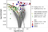 |
Fig. 8. BPT diagram. Large red and blue circles refer to primary (AGN-A) and secondary (AGN-B) nuclei, respectively. All primary and secondary AGNs are above the solid (Kewley et al. 2001) and dashed (Kauffmann et al. 2003) curves, used to separate purely SFGs (below the curves) from galaxies containing AGNs (above the curves, i.e. the Seyfert region of the BPT). The olive curve indicates the locus of z ∼ 2.3 SFGs from (with intrinsic scatter relative to the median curve in light-olive Strom et al. 2017); additional measurements for z > 2.6 SFGs and AGNs are reported with small symbols (see legend and Sect. 6.1 for details). All reported measurements show that the Seyfert area of the BPT is free from contamination by SFGs at any considered redshift, and, therefore, ensure the AGN classification of the newly discovered sources COS1638-B, GS551-B, Eastfield, Mr. West, COS1656-B, and GS10578-B. All AGN-A and B flux ratios are reported in Table A.2. |
For reference, the BPT diagnostic in Fig. 8 also displays the optical line ratio measurements from the remaining type 2 AGN in GA-NIFS (small red circles), for which spectra will be presented in Bertola et al. (in prep.) and Venturi et al. (in prep.). The BPT also presents other measurements from the literature. In particular, there are low-z SDSS galaxies (small grey points), the median locus of SFGs at z ∼ 2.3 from Strom et al. (2017, light-olive curve with intrinsic scatter), and SFGs and AGNs at z > 2.6 recently observed by JWST (from Scholtz et al. 2025; Calabrò et al. 2023). The demarcation lines used to separate galaxies and AGNs at z ∼ 0 from Kewley et al. (2001) and Kauffmann et al. (2003) are also marked in the diagram.
The flux ratios for our primary and secondary AGNs fall well above those of distant (z ≳ 3) star-forming galaxies observed so far (e.g. Sun et al. 2023; Sanders et al. 2023; Nakajima et al. 2023) and occupy the same region as local Seyfert galaxies and AGNs at cosmic noon, providing strong support for their classification as active nuclei. The high [N II]/Hα line ratios suggest that these AGNs reside in metal-enriched environments, as expected for massive systems (Karouzos et al. 2014; Curti et al. 2023); in fact, all our primary AGNs have stellar masses log(M*/M⊙) > 9.8 (see Sect. 5.7). A more detailed discussion about the use of BPT to identify AGNs at z ≳ 2.6 is presented in Sect. 6.1.
5.2. UV emission lines and line ratio diagnostics
Figure 9 shows a comparison between the Lyα emission maps derived from MUSE cubes (top panels) and the [O III] emission observed with NIRSpec (middle panels) for the two GA-NIFS AGNs covered by MUSE observations: GS10578 and GS551. The Lyα maps were created by integrating the emission across the line profiles detected at the position of the X-ray AGN (GS10578) and the close companions (GS551). The Lyα spectral profiles are reported in the bottom panels of the figure. The overlaid contours in the maps mark the emission at different wavelengths, highlighting the presence of the Lyα emitters (LAEs) around the central AGN, which spectral lines are reported with different colours in the bottom panels.
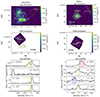 |
Fig. 9. Comparison between Lyα (top) and [O III] emission maps (middle panels) for GS10578 (left) and GS551 (right), and spectra extracted from individual Lyα emitters (bottom). Both MUSE and NIRSpec images have been sampled with 0.05″/spaxel, to ease the comparison between UV and optical emission line spatial distributions. The Lyα maps are integrated over the emission profile at the location of the X-ray AGN, with overlaid contours indicating emissions at different wavelengths and highlighting nearby Lyα emitters. The bottom panels show spectra near the Lyα line for each system, in velocity space with respect to the systemic redshifts of the primary AGN; these spectra were extracted from regions with S/N > 5. In GS10578, two bright Lyα emitters (LAE1 and LAE2) are located ∼20 kpc south of the AGN; a Lyα halo at slightly lower redshift (z = 2.99) previously identified by Leclercq et al. (2017) is also marked with orange contours. GS551 features three Lyα emitters at varying distances up to ∼30 kpc; an even more distant Lyα emitter located ∼80 kpc to the north-east was also identified by den Brok et al. (2020, see their Fig. 2). The contours in the map panels are in steps of 1σ, for LAE_L17 and the GS551 companions, and in steps of 3σ (10σ) for GS10578 (GS551); all contours start from 5σ and are obtained integrating over the velocity channels shown in the bottom spectra according to their colours. These MUSE observations illustrate that GS551 and GS10578 are embedded in dense, complex environments. |
While the MUSE data do not resolve individual [O III] emitters identified by NIRSpec, they reveal extended Lyα nebulae that encompass both the primary and secondary AGNs, stretching several kiloparsecs from the central SMBHs. In GS10578, two prominent Lyα emitters are detected approximately 20 kpc south of the central X-ray AGN, and appear nearly as luminous as the primary AGN itself. These two sources, labelled LAE1 and LAE2, have systemic velocities within a few hundreds of km s−1 of the GS10578-A systemic redshift. Additionally, these two emitters lie ∼50 kpc (and ∼6000 km s−1) from a previously discovered Lyα halo identified by Leclercq et al. (2017, LAE_L17 in the figure).
The MUSE data reveal three additional Lyα emitters in the surroundings of GS551: a faint source located ∼10 kpc to the north (LAE1), a compact source located ∼20 kpc to the south-east (LAE2), and a third ∼30 kpc to the north-west with a clumpy morphology extending for nearly 20 kpc (LAE3). All of these systems share systemic redshifts within a few hundreds of km s−1 of the systemic velocity of GS551-A.
The integrated spectra of the emitters associated with GS10578 and GS551, obtained by summing the spaxels within the outer contours corresponding to S/N = 5, are shown in the bottom panels of Fig. 9. This first qualitative analysis of the archival MUSE data indicate that both GS10578 and GS551 reside in highly complex and dense environments.
We further examined the spectra of each Lyα emitter to determine their ionisation sources. Of the six emitters, only LAE2 associated with GS10578 exhibits additional emission lines beyond Lyα. We fitted the spectrum of LAE2, as well as those of the central X-ray AGN GS10578 and GS551, using Gaussian profiles (described in Sect. 4). The best-fit models for these sources are displayed in Figs. 10 and 11; best-fit parameters are reported in Table A.3.
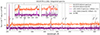 |
Fig. 10. MUSE spectra of GS10578 (coral) and LAE2 (purple). These spectra were obtained by integrating over the regions at S/N > 4 in Fig. 9; for visual purposes, the LAE2 spectrum was shifted vertically, as labelled. The zoom-in insets show the same spectra in the vicinity of the lines used in the UV diagnostics used to classify LAE2 as an AGN (Fig. 12), together with 3σ errors for the LAE2 spectrum (grey area, mostly highlighting the position of strong sky line residuals). |
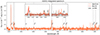 |
Fig. 11. MUSE spectra of GS551 (coral), showing AGN-ionised lines, according to UV diagnostics (Fig. 12). These spectra were obtained by integrating over the regions at S/N > 4 in Fig. 2; for visual purposes, the LAE2 spectrum was shifted, as labelled. The zoom-in insets show the same spectra in the vicinity of the lines used in the UV diagnostics, together with 1σ errors for the LAE2 spectrum (green curve, mostly highlighting the position of strong sky line residuals). |
High-ionisation lines such as C IVλλ1548, 51 and He IIλ1640 lines are detected in the spectra of the two X-ray sources as well as in the LAE2 spectrum although at lower significance. In particular, LAE2 shows a strong He II line detected at S/N ∼ 20; the C IV and C III] lines are affected by sky line subtraction residuals, but their detections are associated with a reasonable significance (> 5σ). The coronal line (CL) N Vλλ1239, 43 are observed only in the X-ray AGN, but its absence in LAE2 does not exclude AGN activity from this source (e.g. Maiolino et al. 2024b). To explore the ionisation source in LAE2, we used the UV diagnostic diagram involving C IV/C III] versus (C III] + C IV)/He II, as presented by Nakajima & Maiolino (2022) and Feltre et al. (2016).
Figure 12 shows the positions of LAE2, GS10578, and GS551 in the UV diagnostic, together with nine additional X-ray AGNs at redshifts z = 2.6 − 4 from other surveys. The flux ratios of five of them have been obtained from the analysis of publicly available VIMOS spectra from the VANDELS programme (McLure et al. 2018), which provides some of the deepest spectra of intermediate redshift galaxies available to date. In particular, among the X-ray AGNs identified by Saxena et al. (2020) and Mascia et al. (2023) in VANDELS, we considered the obscured AGNs (i.e. without BLR emission in their UV spectra) with enough S/N to derive the flux ratios required for the UV diagnostic (i.e. excluding CDFS 019505). The fit analysis was performed using the same strategy presented for the MUSE data; the inferred flux ratios are reported in Table A.4. In addition to the five AGNs from VANDELS, we included in Fig. 12 the X-ray AGN UDS24561 at z ∼ 3 discovered by Tang et al. (2022), and the sources CDFS-057 (z = 2.56), CDFS-112a (z = 2.94), and CXO 52 (z = 3.288) from Dors et al. (2014), using the flux ratios tabulated in the original papers. Figure 12 also displays the flux ratios obtained from composite spectra of AGNs at z ∼ 3 from Alexandroff et al. (2013, brown and light-brown crosses, indicating respectively their Class A and Class B AGN sources), and Le Fèvre et al. (2019, orange cross, from the stacked spectrum of seven X-ray obscured AGNs).
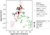 |
Fig. 12. UV diagnostic diagram. Small green and red empty symbols represent model predictions for SFGs and AGNs, respectively, from Nakajima & Maiolino (2022). See the legend for details about model parameters. Large circles refer to the MUSE measurements of the three sources in our sample, as labelled; MUSE resolution does not allow us to separate the contribution of primary and secondary AGNs, but GS551 and GS10578 line ratios are likely dominated by the primary (brightest) AGN. The figure also shows individual X-ray AGNs (diamonds) and measurements from stacked AGN spectra (crosses), as well as SFGs at z ∼ 3 from the literature (green squares; see Sect. 5.2). GS551, GS10578 and LAE2 occupy the AGN region of the diagram. |
Non-active SFGs with strong high ionisation UV lines appear exceedingly rare in spectroscopic surveys (e.g. Amorín et al. 2017; Mascia et al. 2023). To represent them in Fig. 12 we considered the catalogue of VANDELS sources in the UDS field by Talia et al. (2023), and selected the sources for which at least one line is detected at S/N > 3 among C IV and C III] (to derive at least upper or lower limit for the C IV/C III]), and at least two lines are detected at S/N > 3 among C III], C IV and He II (to derive upper or lower limits for the (C IV + C III])/He II). These SFGs at z ∼ 3 are represented with green squares. We also plot the models of AGNs and SFGs as red stars and green circles, respectively, from Nakajima & Maiolino (2022). According to this UV diagnostic, LAE2 can be identified as an AGN emitter, sharing line ratios similar to those of GS10578, GS551, and other X-ray AGNs, as well of models of AGNs.
This UV diagnostic, therefore, confirms the presence of a third AGN in the GS10578 system, in addition to the AGN-A and AGN-B identified in the NIRSpec data. A more detailed discussion about the use of UV diagnostics is presented in Sect. 6.2.
5.3. AGN bolometric luminosities
For all AGNs detected with NIRSpec, we computed the bolometric luminosities from the narrow Hβ line, under the assumption that this emission comes from the NLR; bolometric corrections were computed using Eq. (3) of Netzer (2019), assuming a mean accretion disc inclination of 56°. These luminosities were preferred to the [O III]-based ones, because the latter are more dependent on the SMBH properties and the ionisation parameter (Netzer 2019); for completeness, all [O III] (and Hα) luminosities are reported in Table A.2 for each target presented in this work.
All Hβ luminosities were corrected for extinction, using the measured Balmer decrements reported in Table A.2 and assuming a Cardelli et al. (1989) extinction law. For the AGN in LAE2 detected with MUSE, we computed the bolometric luminosity from an upper limit on the (undetected) continuum emission at 1400 Å, using Eq. (3) by Netzer (2019), adopting the same accretion disc inclination mentioned above. We note that its He II luminosity is comparable with that of GS10578-A; this might suggest that LAE2 and the primary AGN have comparable bolometric luminosities.
All bolometric luminosities are reported in Table 1. As there is no rigorous way to estimate the uncertainties in the bolometric corrections introduced by Netzer (2019, see their Sect. 2.4), we preferred to not include error bars on the estimated bolometric luminosities; these should therefore be considered as order-of-magnitude estimates.
5.4. Ionisation source
For two very close AGN pairs, GS551-A and -B with projected separation of 0.7 kpc, and GS10578-A and -B with separation of 4.7 kpc, we checked whether the primary AGN can power the emission in the companion galaxy. Specifically, we tested whether the line emission in GS551-B and GS10578-B can be explained by an external ionisation source (i.e. AGN-A), or requires an intrinsic source (i.e. a secondary AGN).
Following Keel et al. (2012), we derived a lower limit to the incident ionising flux required for a line emitter taking into account the observed surface brightness in the recombination line Hβ, and its distance from the primary AGN. No corrections for projection effects are considered, to obtain conservative estimates: a given companion will always lie farther from the nucleus of the primary AGN than our projected measurement, and hence require a higher incident flux. In a simple approximation, we considered the companion to be circular in cross-section as seen from the nucleus, so its solid angle is derived as θ = 2arctan(r/d), where r is the radius of the emitting region and d is the angular distance from the primary AGN. The required ionising luminosity is given from the observed quantities as
 (1)
(1)
where L(Hβ) is the Hβ luminosity of the companion, kbol is the bolometric correction from Netzer (2019, Sect. 5.3), γ = 0.14 is the fraction of bolometric to ionising luminosity (considering the mean radio-quiet SED, following Keel et al. 2019), and θ is the subtended angle (in steradian). This required ionising luminosity has to be compared with the incident ionising luminosity coming from the primary AGN: Linc = Lbol × γ (following Keel et al. 2019).
For GS551-B, we obtained a required Lion > 4 × 1045 erg s−1, slightly higher than the incident Linc = 1045 erg s−1. Although Linc and Lion are of the same order of magnitude, and we cannot definitely exclude the possibility of an external AGN ionisation, the latter scenario is very unlikely. In fact, Lion has to be considered as a lower limit: assuming a 3× larger physical (i.e. de-projected) distance, we would obtain 10× higher Lion, definitely incompatible with external AGN ionisation source. Therefore, our results are likely compatible with an intrinsic ionisation, hence with the presence of a secondary AGN.
For GS10578-B, we obtained a required Lion > 3 × 1045 erg s−1, to be compared with the incident Linc ≈ 6 × 1043 erg s−1. In this case, the ionising flux coming from the primary AGN is not enough to explain the emission in GS10578-B; we can therefore conclude that the latter is associated with a secondary AGN.
For the remaining sources, the required ionising luminosity is 10 s–103 times higher than the incident luminosity, definitely excluding the possibility of an external AGN ionisation source. Similar computations are not required for the pair LAE2 – GS10578-A, as the two sources have comparable emission line luminosities in the UV (Table A.3); moreover, they are separated by 28 kpc.
5.5. Shock ionisation
We also tested the possibility that shocks could ionise the gas in the companions. Following Perna et al. (2020), we used the shock model predictions of Hα luminosity from MAPPING V (Sutherland & Dopita 2017), with magnetic field values in the range 10−4 − 10 μG, shock velocities in the range 100−1000 km s−1, pre-shock densities in the range 1−10 cm−3 (to obtain [S II]-based post-shock electron density in the range 50 − 4000 cm−3, in line with observations at high-z, e.g. Rodríguez Del Pino et al. 2024; Lamperti et al. 2024), and assuming a metallicity of 1 Z⊙. These predicted luminosities are a factor of 4-to-2 dex smaller than our measurements (Table A.2); therefore, we conclude that shock ionisation cannot be responsible for the emission in any of our secondary AGN sources.
5.6. X-ray analysis of COS1638
X-rays have proven inefficient in detecting dual AGNs at z > 1 due to the limited sensitivity and angular resolution of current X-ray facilities (Sandoval et al. 2023). Nevertheless, here we investigate the X-ray morphology of one of our dual AGN system, covered with Chandra observations. Additional information about X-ray emission of all other systems is presented in Appendix B.
We inspected the X-ray morphology of the dual AGNs associated with COS1638 through the Chandra exposures of the COSMOS-Legacy survey. Given the survey strategy (Elvis et al. 2009; Civano et al. 2016), the target is placed at different distances from the Chandra aim point in each observation (each with same exposure time), with an off-axis angle of at least θ ∼ 3.5′. As a result, the single-exposure point spread function (PSF) at the position of the primary AGN is of at least ∼1.2″. Figure 13a shows the 0.5−7 keV (observed-frame, sub-binned and smoothed) Chandra image obtained in the best conditions (obsID 15253, 50 ks, θ ∼ 3.5′, PSF ∼ 1.2″), with overlayed [O III] contours.
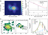 |
Fig. 13. COS1638 X-ray emission. (a) Chandra image (obsID 15253) in the 0.5−7 keV observed-frame energy band, smoothed and sub-binned (1/2 pixel binning, i.e. 0.25″ pixel scale) for visualisation purposes. NIRSpec [O III] and X-ray contours are overlayed in black and in red, respectively. (b) radial profile of COS1638 in obsID 15253 extracted from the native-pixel event file, after masking the pixels affected by the PSF hook, using a set of 5 annuli (δr ≃ 0.5″) centred on the peak of the source emission (which corresponds to COS1638-A). The radial profile was fit with the radial PSF model (see Sect. 5.6) plus a constant set to the measured background level (model: PSF+constant). The red solid line shows the best fit, the blue dash-dotted line shows the simulated PSF profile, while the black dotted line shows the measured background level. The observed radial profile shows hints (∼2σ) of an X-ray excess at the distance of COS1638-B (∼2−3 native Chandra pixels, corresponding to ∼1.2″). (c) 0.5−7 keV images of the simulated PSFs at the positions of COS1638-A (marked with a ‘+’) and COS1638-B (‘x’). The lettered boxes show the extraction regions of the radial profiles in panel d. The magenta region shows the position of the hook feature, whose corresponding pixels were masked in the Chandra data before extracting the radial profiles. (d) 0.5−7 keV (observed energy range) radial profiles of COS1638 extracted from ObsID 15253, from masked (magenta) and unmasked (green) data. The black solid line marks the total X-ray profile obtained from fitting the data with the two PSFs (dash-dotted and blue dashed lines for COS1638-A and COS1638-B, respectively) and the background (grey dashed line). Thus, the X-ray morphology overall hints at the presence of a second peak at the position of COS1638-B. |
Thus, we investigated the X-ray radial profile of COS1638 in the Chandra exposure obsID 15253, using the Chandra Ray Tracer (ChaRT v.25) online tool (see Fig. 13 for details). We simulated the Chandra PSFs at the positions of COS1638-A and COS1638-B with ChaRT, feeding the ray-tracing code with the respective target and aim-point coordinates, the exposure time and the respective 0.5−7 keV source spectrum. The source spectrum extracted from this observation is integrated over the two AGN components and dominated by COS1638-A and, thus, we used its best fit for COS1638-A. For COS1638-B, we built an obscured powerlaw model (NH = 5 × 1023 cm−2), given that it is a type 2 AGN, setting the X-ray flux as equal to that obtained converting its [O III] luminosity through the relation of Lamastra et al. (2009). We ran 50 ChaRT simulations for both PSFs, each of which was then projected on the detector plane using MARX v.5.5.2 (Davis et al. 2012). We merged the output of MARX with the task dmmerge in CIAO v4.15 (Fruscione et al. 2006) to best reproduce both Chandra PSFs. We show the 0.5−7 keV maps of the two PSFs in Fig. 13c.
It is known that the PSF of both cameras on board Chandra presents a hook-like feature dependent on the observation characteristics (Koss et al. 2015) that ChaRT and MARX do not account for. We thus used the make_psf_asymmetry_region task of CIAO to uncover the pixels affected by such an asymmetry and mask them in the observation event file. We show the asymmetry region overlayed to the PSF of COS1638-A for clarity. We then extracted the radial profile of the entire system, from the event file masked for the PSF asymmetry, by using a set of 5 annuli (δr ≃ 1 pix ≃0.5″) centred on the peak of the source emission (which corresponds to COS1638-A) and fitted it with the radial PSF model (obtained from the PSF of COS1638-A) plus a constant set to the measured background level (model: PSF A+constant), using Sherpa 4.15.1 (Burke et al. 2023). Background contribution was estimated from a 15″-radius source-free circle in the proximity of our target. Figure 13b shows the 0.5−7 keV (observed-frame) X-ray profile from the data and the best fit from Sherpa. The observed profile shows hints (∼2σ) of an X-ray excess at the distance of COS1638-B (∼2−3 native Chandra pixels, corresponding to ∼1.2″). We also repeated this exercise restricting the extraction areas to those shown in Fig. 13c, to reduce noise contamination. We show in Fig. 13d the radial profile from the Chandra data, both masked and unmasked for the PSF asymmetry, the total radial profile of the two PSFs and the contribution of each PSF. Hence, despite the degraded PSF due to the off-axis position, the X-ray morphology suggests the presence of a second peak at the position of COS1638-B.
We tested the possibility of this peak being due to high SF activity, rather than to a secondary AGN; the measured SFR ≃ 1200 M⊙ yr−1 (see Appendix B) translates to L[0.5−8 keV] ≃ 8 × 1042 erg s−1 (Mineo et al. 2014). Thus, we addressed the detectability of a starburst galaxy with such a high SFR by assuming a reasonable spectral shape for the X-ray binary emission (Yang et al. 2020, and references therein). The expected X-ray flux of such starburst galaxy would be almost one order of magnitude lower than the flux limit of COSMOS-Legacy and subsequently undetectable in obsID 15253 alone. Thus, the X-ray emission of COS1638 supports the presence of a secondary AGN in COS1638-B.
5.7. Stellar masses of AGN host galaxies
To infer the stellar masses of the host galaxies of the multiple AGNs presented in this work, we exploited their multi-wavelength information.
To study the physical properties of the stellar populations in Eastfield and Mr West (Fig. 5), we analysed the prism (0.6−5.3 μm) NIRSpec IFS observations in a spaxel-by-spaxel basis following the method described in Pérez-González et al. (2023), and adapted to the modelling of NIRSpec IFS data by D’Eugenio et al. (2024). These data were reduced following the same procedure described in Sect. 3. Based on this method, we derived integrated stellar masses of ∼109 M⊙ for both AGN host galaxies, by adding all the spaxels associated with these systems. In particular, for Mr West we considered a circular region with r = 0.2″ centred at the position of the nucleus (AGN-B in Fig. 5), while for Eastfield we considered a larger (r = 0.3″) region to encompass its ring-shaped structure (reddish region in Fig. 5). More detailed analysis of the physical properties of the stellar populations in this very complex system is presented in Pérez-González et al. (2024); here we stress that the mass measurements depend only slightly on the chosen apertures.
For all other systems observed with NIRSpec IFS, we analysed through spectral energy distribution (SED) fitting the COSMOS (GOODS-S) UV-to-NIR multiwavelength photometry collected by Weaver et al. (2022) and Merlin et al. (2021), and the far-IR data by Jin et al. (2018) and Shirley et al. (2021). We also included in the analysis the ALMA sub-millimetre detections (for COS1638) and 3σ upper limits (for all other sources). For the Lyα emitter in the vicinity of GS10578, associated with the AGN-C (Fig. 9, top left), we used publicly available NIRCam and HST measurements collected by Rieke et al. (2023).
We modelled the SED with the Code Investigating GALaxy Emission (CIGALE v0.11.0, Boquien et al. 2019), a publicly available state-of-the-art galaxy SED-fitting software. This code disentangles the AGN contribution from the emission of the host by adopting a multicomponent fitting approach and includes attenuated stellar emission, dust emission heated by star formation, AGN emission (both primary accretion disc emission and dust-heated emission), and nebular emission (see Circosta et al. 2018, 2021 for further details). The more detailed SED analysis will be presented in Circosta et al. (in prep.). Here we report that the primary AGNs are hosted in massive (≈1011 M⊙) galaxies; the secondary and tertiary AGN hosts have smaller masses, in the range 108 − 1010 M⊙ (see Table 1). Unfortunately, no M* measurements can be obtained for COS1638-B, GS551-B and GS10578-B, as they are not resolved as individual sources in the above mentioned catalogues (they are too close to the primary AGN): indeed, the photometry used for the primary AGN host may be contaminated by these companions; as a result, the estimates we obtain may include the contribution of both components.
A separate handling is required for the type 1 COS1638-A. Stellar mass estimates in the range 108 − 1012 M⊙ are reported in the literature for the host galaxy of the primary AGN (e.g. Jin et al. 2018; Weaver et al. 2022); this divergence is likely due to the non-thermal AGN emission dominating the optical continuum (Circosta et al., in prep.), which is precluding an SED-based estimate of M*. However, an order of magnitude estimate of the stellar mass can be obtained considering our MBH = (4 ± 1)×108 M⊙ measurement (see Appendix B) and assuming the local black hole mass-stellar mass relation (Kormendy & Ho 2013), M* ∼ 1011 M⊙. A further independent estimate can be obtained for both primary and secondary AGN hosts from the far-IR-based dust mass Mdust ∼ 1011 M⊙ reported in Liu et al. (2019) and referring to the dual AGN system (because of the poor spatial resolution of far-IR data). Archival ALMA data (2016.1.00463.S, PI: Y. Matsuda) tracing far-IR emission at ∼1 mm shows that COS1638-B is brighter than the primary AGN host (62% of the emission comes from the AGN-B host; see Appendix B). Assuming that 62% of the dust mass is due to the AGN-B host, and considering a conservative Mdust/M* = 0.02 ± 0.01 (Donevski et al. 2020) we obtained log(M*/M⊙) ∼ 10.9 ± 0.4, for COS1638-A, and ∼11.1 ± 0.4, for COS1638-B. We note that the far-IR properties of this system, as well as its X-ray properties and optical emission profiles and line ratios appear to be similar to the BR1202–0725 (Zamora et al. 2024) dual AGN systems.
6. Discussion
6.1. AGN classification based on optical diagnostics at z > 2.6
Several approaches have been proposed to test the presence of an AGN from the study of rest-frame optical spectra. Among them, the use of optical diagnostic diagrams such as the BPT (Baldwin et al. 1981, see our Fig. 8), and the detection of forbidden high ionisation lines, known as CLs, with ionisation potentials IP > 54.4 eV (the He II edge; e.g. Oliva et al. 1994; Moorwood et al. 1997). In this section we discuss their possible use and reliability for the AGN classification of the newly discovered sources COS1638-B, GS551-B, Eastfield, Mr. West, COS1656-B, and GS10578-B.
Usually, [Ne V] λ3435 and [Fe VII] λ6087 are the most prominent forbidden CLs in the optical range. Unfortunately, [Ne V] is not covered by our NIRSpec observations. The [Fe VII] line, which is the brightest CL in the 3500 − 7500 Å range, is usually only 1−10% of the strength of [O III] (Murayama & Taniguchi 1998; Mingozzi et al. 2019). Moreover, quantitative studies on the prevalence of CLs, even in the local Universe, remain limited. CLs are thought to be more common in type 1 AGNs (e.g. Lamperti et al. 2017; Cerqueira-Campos et al. 2021). Interestingly, however, CLs remain undetected in near- and mid-infrared wavelength regions of the well-known local type 1 AGNs observed with JWST, Mrk 231 (Ulivi et al., in prep.; Alonso Herrero et al. 2024). This underscores the challenges in relying on CLs for AGN classification (see also Perna et al. 2024).
The [Ne V] and [Fe VII] high ionisation lines are not detected in our newly discovered AGN sources, nor in their composite spectrum ([Fe VII]/[O III] ≲ 3%; see Fig. C.1). This is likely because of their type 2 nature; in fact, a composite spectrum of six X-ray detected, type 2 AGNs in our sample similarly shows no clear evidence of CLs although they are much brighter than the secondary AGN (Fig. C.2). However, we stress that the prevalence of CLs in the AGN population is unconstrained yet, at any redshift. Therefore, other diagnostics are considered in this work to identify AGN emission in our sources.
The BPT diagnostic provides an unambiguous classification for the newly identified sources in Figs. 3–7, as their flux ratios fall into the Seyfert region of the diagram (see Fig. 8). This area is deemed free from contamination by SFGs, according to the latest observational and theoretical findings. On the one hand, the contaminating processes that may mimic AGN-like signatures, that is the presence of post-AGB stars (e.g. Wylezalek et al. 2018), can be excluded thanks to the very high [O III]/Hβ and Hα equivalent width (EW). In particular, the measured EW(Hα) of 15 − 150 Å (see Table A.2) are significantly higher than those expected for post-AGB stars (< 3 Å, e.g. Belfiore et al. 2016). On the other hand, hot young stars cannot be responsible for Seyfert-like line ratios, according to both theoretical predictions (e.g. Topping et al. 2020; Runco et al. 2021; Nakajima & Maiolino 2022) and observations: recent JWST observations proved that non-active galaxies at z > 2.6 can have high [O III]/Hβ but relatively low [N II]/Hα with respect to local Seyfert and active galaxies at high-z (e.g. Sanders et al. 2023; Nakajima et al. 2023; Sun et al. 2023). The BPT diagnostic in Fig. 8 shows a compilation of SFGs at z = 2.6 − 7, from the CEERS (Calabrò et al. 2023) and JADES (Scholtz et al. 2025) surveys. These sources avoid the Seyfert region of the BPT, and tend to occupy the same locus as SFGs at cosmic noon (light-olive shaded area in the figure). On the contrary, high-z AGN can populate both the Seyfert region and the locus of non-active galaxies, as proved by our measurements from GA-NIFS (red circles, associated with X-ray detected AGNss and broad-line AGNs) and from JADES measurements (orange points, classified as AGNs on the basis of additional diagnostics, from Scholtz et al. 2025; see also e.g. Harikane et al. 2023; Kocevski et al. 2023; Maiolino et al. 2024a; Duan et al. 2024).
Summarising, AGNs at 3 ≲ z ≲ 6 can have (i) optical line ratios very similar to those of local Seyfert and z ∼ 2 active galaxies, or (ii) line ratios similar to SFGs at z > 1. The former, with log([N II]/Hα) ≳ −0.5 and log([O III]/Hβ) ≳ 0.75, are more likely hosted in massive systems (see Table A.2). The latter, with log([N II]/Hα) ≲ −1 and log([O III]/Hβ) ≳ 0.75, are likely hosted in galaxies with smaller masses (and lower metallicity, e.g. Scholtz et al. 2025). This dichotomy aligns with predictions from photoionisation models developed over the last decades (see e.g. Dors et al. 2024 and references therein). Most importantly, the Seyfert region of the BPT diagram is free from contamination by SFGs. All arguments collected in this section reinforce the BPT-based AGN classification for the newly identified sources shown in Figs. 3–7.
6.2. AGN classification based on UV diagnostics at z > 2.6
Direct observations of high-ionisation lines in the UV regime, such as N Vλλ1239, 43, C IVλλ1548, 51, He IIλ1640, also in combination with other UV transitions, serve as robust indicators of AGN activity in distant galaxies (e.g. Mascia et al. 2023; Scholtz et al. 2025; Maiolino et al. 2024c). In this section we focus on the use of N V, a very high ionisation line (IP ∼ 80 eV), and the UV diagnostic diagram C IV/C III] versus (C III] + C IV)/He II (Fig. 12) to distinguish between AGN and SF ionisation in high-z sources, and confirm the presence of an AGN in LAE2.
As noted by Maiolino et al. (2024b), the absence of N V cannot definitively rule out AGN activity, as its intensity relative to other UV lines varies significantly. For instance, N V is a few times stronger than He II in the X-ray detected AGN GS551 (see Fig. 11, Table A.3), but it is not detected in other X-ray AGNs reported in the literature (see e.g. Law et al. 2018; Tang et al. 2022). The ratio N V/C IV can vary from 0.01 to 1 in type 1 AGNs (see Fig. 6 in Maiolino et al. 2024b), and is often < 1 in obscured AGNs at z > 2 (e.g. Silva et al. 2020; Mignoli et al. 2019; see also Tables A.3, A.4). Consequently, the non-detection of N V in the MUSE spectrum of LAE2 does not exclude the presence of an accreting SMBH in this source.
To test the reliability of the UV diagnostic diagram C IV/C III] versus (C III] + C IV)/He II presented in Fig. 12, we incorporated measurements for nine X-ray detected AGNs at z ∼ 2.6 − 4 and flux ratios from composite spectra of AGNs at z ∼ 3 reported in the literature. By including these additional measurements, we ensured a robust comparison between UV line ratios observed in LAE2 and those of confirmed AGNs. The flux ratios of these bona fide AGNs align closely with those of LAE2, as well as with predictions for AGN ionisation models by Nakajima & Maiolino (2022, see also Gutkin et al. 2016).
In contrast, SFGs with strong high-ionisation UV lines appear exceedingly rare in spectroscopic surveys (e.g. Amorín et al. 2017; Mascia et al. 2023). To display their population in Fig. 12, we considered the catalogue of VANDELS sources in the UDS field by Talia et al. (2023), and selected galaxies where the detected UV lines, or a combination of detections and upper limits, allowed their inclusion in the diagnostic plot. Figure 12 shows that all SFGs have upper limits that point towards the locus of Nakajima & Maiolino (2022) predictions for SF systems (see also Feltre et al. 2016). Most of the ∼900 sources in the Talia et al. (2023) VANDELS catalogue cannot be reported in this diagnostic diagram, as the UV emission lines are usually very faint or undetected even with > 20 hours integration time (see also Mascia et al. 2023).
Well detected C IV, C III] and He II have been reported in the literature for a few non-active galaxies (e.g. Le Fèvre et al. 2019; Mascia et al. 2023); their flux ratios cover the bottom-right part of the UV diagram in Fig. 12, as shown by Nakajima et al. (2018, see their Fig. 11). Moreover, a handful of sources classified as local dwarf galaxies (Berg et al. 2016; Senchyna et al. 2017) and z ∼ 2 compact SF galaxies (Amorín et al. 2017) can reside in the AGN region of the UV diagnostic (see Figs. 11 and 14 in Nakajima et al. 2018). Nevertheless, these peculiar sources can typically be distinguished from AGNs by their strong low-ionisation lines such as [Si III]λλ1883, 92 and O III]λλ1661, 66 (e.g. O III]/C IV > 1; see Fig. 4 in Senchyna et al. 2017, Fig. 2 in Berg et al. 2016, Supplementary Fig. 4 in Amorín et al. 2017). Such low ionisation lines are usually faint or undetected in obscured AGNs at high-z (and in LAE2; see Tables A.3 and A.4; see also Talia et al. 2017), consistent with theoretical predictions (e.g. Nakajima & Maiolino 2022). In Tables A.3 and A.4 we reported additional UV line ratios usually taken into account in alternative UV diagrams commonly adopted in the literature (see e.g. Mignoli et al. 2019; Mingozzi et al. 2024); also these alternative UV diagnostics show similarities between LAE2 and the X-ray sources collected in this work, and therefore confirm the AGN classification for LAE2.
In conclusion, LAE2 is the only source undetected in X-ray sitting at the position of X-ray AGNs at similar redshifts (from this study, and from Dors et al. 2014; Saxena et al. 2020; Tang et al. 2022; Mascia et al. 2023; Le Fèvre et al. 2019); all SFGs from VANDELS are instead below the location of X-ray AGNs. LAE2 also differs from local dwarf galaxies and compact SFGs at the cosmic noon in terms of O III]/He II. All evidence, including UV line diagnostics, comparisons to X-ray AGNs, and the absence of strong low-ionisation features, strongly supports the classification of LAE2 as an AGN.
6.3. Dual AGN fraction at z ∼ 3
The fraction of dual AGN systems in the early Universe provides crucial insights into galaxy mergers and the growth of SMBHs. Moreover, AGN pairs are pivotal for forecasting gravitational wave background levels and event rates in PTA experiments and for the future LISA mission. Cosmological simulations, such as those homogenised by De Rosa et al. (2019) and, more recently, by Puerto-Sánchez et al. (2025), predict dual AGN fractions of 1%−6% for physical separations d3D < 30 kpc and luminosities Lbol > 1043 erg s−1 in the redshift range z ∼ 1 − 6 (see also Steinborn et al. 2016; Rosas-Guevara et al. 2019; Chen et al. 2023). Volonteri et al. (2022) reported an expected fraction ∼4% for dual AGNs at z ∼ 3 with slightly stricter criteria of d3D < 30 kpc and Lbol > 1044 erg s−1. However, to align the threshold criteria of these theoretical works with the GA-NIFS observations, we should consider projected separations dp < 10 kpc and even higher bolometric luminosities (see Table 1). In fact, all theoretical works show that predictions are sensitive to the threshold criteria used to define the parent population and the number of duals, in addition to the specific dynamical and physical implementations and numerical methods.
To ensure the match between GA-NIFS observations and predictions, we presented in Fig. 14 the AGNs extracted from the Horizon-AGN simulation, using an identical approach to those presented in Volonteri et al. (2022), but extended to higher redshifts (z ∼ 6) and considering dual AGNs with projected separations dp < 10 kpc and < 30 kpc and different AGN luminosities. The newly derived fractions at z ∼ 2 − 5 for the most luminous dual AGNs are slightly higher compared to earlier reports in the literature (e.g. De Rosa et al. 2019). This discrepancy can be attributed to three key factors: (i) the fraction increases if the secondary is allowed to be fainter than the primary (see also the blue curve in Fig. 16 of Volonteri et al. 2022), (ii) the most luminous AGNs are more likely hosted in massive galaxies, which, at high redshift, are often found in over-dense regions and hence more likely to have close active companions, and (iii) no cuts were imposed on the mass of the SMBHs, something that is often done in cosmological simulations to improve the purity of the sample, but at the cost of decreasing completeness (e.g. Puerto-Sánchez et al. 2025). Further details regarding the assumptions considered for deriving the predictions reported in the figure are discussed in Appendix D.
Figure 14 also shows the fraction of dual AGNs derived from our JWST observations, of ∼20 − 30%. Specifically, the lower value is inferred considering only the three confirmed dual AGNs systems out of the 16 AGNs in GA-NIFS, hence excluding the GS551 and Jekyll systems; the higher value is instead derived also considering these two candidate dual AGN systems. Our inferred fractions are moderately above predictions (∼10%) from cosmological simulations that mimic our observational criteria, that are: dp < 10 kpc, log(Lbol, A) > 45 (for the primary AGN and the parent population) and log(Lbol, B) > 44 (for the secondary AGN), shown with a blue dashed curve Fig. 14. As expected, our measurements significantly exceed the predicted fractions obtained considering log(Lbol, A) and log(Lbol, B) > 43, and d3D < 30 kpc (grey curve), consistent with previous works (e.g. De Rosa et al. 2019; Rosas-Guevara et al. 2019; Volonteri et al. 2022).
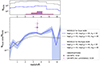 |
Fig. 14. Dual AGN fraction as a function of redshift. The purple square shows the inferred dual AGN fraction from GA-NIFS observations, for the three newly discovered dual AGNs; instead, the violet symbol displays the fraction obtained also considering the two candidate dual AGNs; both measurements include 1σ Poisson errors for small numbers. The different curves represent the predicted AGN fractions obtained from an extension of the Volonteri et al. (2022) simulations up to z ∼ 6, passing different threshold criteria (as labelled). Notably, the figure shows that the GA-NIFS measurements moderately exceed the predictions obtained for thresholds that mimic our observational criteria, hence with projected distances dp < 10 kpc, log(Lbol, A) > 45 (for the primary AGN and the parent population) and log(Lbol, B) > 44 (for the secondary AGN), shown with a blue dashed curve (and Poissonian 1σ intervals in lightblue). The top panel shows the parent sample distributions of GA-NIFS sources (purple histogram) and simulated AGNs (blue for log(Lbol, A) > 45, grey for log(Lbol, A) > 43); we note that simulations at z > 5 suffer from poor statistics. |
We also considered the predictions for dual and multiple AGN systems with d3D < 30 kpc (black dotted curve) and dp < 10 kpc (blue dotted curve), taking into account that (i) for GS10578 and GS551 we could investigate the presence of additional active companions at larger distances from the primary AGN thanks to MUSE observations, and that (ii) we actually discovered the GS10578 triple AGN system with projected separations dp = 4.7 kpc (AGN-A, B) and dp = 28 kpc (AGN-A, C). Also in these cases, Horizon-AGN simulations provide fractions ≲10% at z ∼ 3.
It is important to note that different simulations employ varying models for galaxy and black hole physics, leading to discrepancies in predicted AGN and dual AGN populations. These differences include the initial mass of the BH seeds, seeding conditions in galaxies, BH accretion, AGN and stellar feedback, as well as the implementation of dynamical friction from gas, stars, and dark matter particles. Additionally, simulation resolution, volume, and subgrid prescriptions influence the predictions (e.g. Habouzit et al. 2021). The evolution of the dual AGN fractions over time also depends on the single and dual AGN selection criteria (AGN luminosity, SMBH mass, host stellar mass). All these factors complicate direct comparisons with observations. Puerto-Sánchez et al. (2025) examined various simulations (Illustris, Genel et al. 2014; Vogelsberger et al. 2014; TNG50, TNG100, TNG300, Pillepich et al. 2018; Nelson et al. 2019; Horizon-AGN, Dubois et al. 2016; Volonteri et al. 2016; EAGLE, Schaye et al. 2014; Rosas-Guevara et al. 2019; SIMBA, Davé et al. 2019; Thomas et al. 2019; BlueTides, Feng et al. 2016; and Astrid, Ni et al. 2022; Bird et al. 2022), highlighting the impact of different modelling choices on AGN demographics. The simulations analysed provide dual AGN fractions between 1 and 6% at z ∼ 3 for AGNs with Lbol, A, B > 1043 erg s−1 at physical distances d3D ≤ 30 kpc (see their Fig. 2). These fractions remain nearly unchanged for luminosities > 1044 erg s−1 (see their Fig. B1). Unfortunately, their results are not directly applicable to GA-NIFS due to the different luminosity thresholds (and lack of SMBH and host stellar mass estimates) in our sample. Nevertheless, Puerto-Sánchez et al. (2025) showed that predicted dual AGN fractions remain relatively stable across simulations (within a factor of ∼2 at z ∼ 3), unlike the absolute number densities of single and dual AGNs, which can vary by a few orders of magnitude. In practice, while the overall AGN population has a stronger dependence on how AGNs are modelled in the simulations, the dual AGN fraction is is less dependent on specific choices. For instance, the SIMBA simulation (Davé et al. 2019; Thomas et al. 2019) models BH accretion inspired by loss of angular momentum through torques, whereas Horizon-AGN adopts the Bondi-Hoyle-Lyttleton formalism. The two simulations also adopt different BH seeding methods (i.e. one using a fixed stellar mass threshold, and the other is based on local stellar density); yet their predicted dual AGN fractions differ by less than a factor of 2 (see Figs. 2 and B.1 in Puerto-Sánchez et al. 2025). This suggests that the comparison presented in Fig. 14 between observations and predictions could be broadly valid across different simulation frameworks, albeit with some inherent uncertainties.
In summary, our results point to the presence of a large population of dual AGNs in the early Universe, up to ∼20 − 30% of the total number of active galaxies. This fraction is moderately above predictions (∼10%) from cosmological simulations that mimic our observational criteria (blue dashed curve in Fig. 14). However, the limited number of observed systems (two dual AGNs and two candidate dual AGNs within dp ≲ 10 kpc, and a triple AGN within dp < 30 kpc, out of 16 AGN systems) precludes us from conclusively determining whether Horizon-AGN cosmological simulations underestimate the number of dual AGNs at high-z. Moreover, while our comparison with Horizon-AGN provides valuable insights, it is important to acknowledge that the predicted dual AGN fraction can vary slightly across different cosmological simulations. A comprehensive study of these variations would require a detailed analysis of each simulation’s specific parameters and implementations, which is beyond the scope of this work.
6.4. Towards a possible revised understanding of AGNs at high-z
Our results suggest a substantial population of dual AGNs in the early Universe, with fractions reaching ∼20%−30%, moderately exceeding our newly extracted predictions from the Horizon-AGN cosmological simulations (∼10%) tailored to our observational criteria. Although the limited GA-NIFS sample size precludes definitive conclusions about whether simulations systematically underestimate dual AGN fractions, we note that our findings suggest that multiple AGN systems are more prevalent than previously identified in earlier observational efforts (e.g. Silverman et al. 2020; Shen et al. 2023; Sandoval et al. 2023).
Recent observational studies further support this view, suggesting that multiple AGN systems may indeed be more frequent than previously thought (e.g. Lemon et al. 2022; Yue et al. 2023; Maiolino et al. 2024a; Spingola et al. 2019; Matsuoka et al. 2024; Pensabene et al. 2024; Perna et al. 2025; Travascio et al. 2025). In particular, Spingola et al. (2019) and Schwartz et al. (2021) found evidence for a sub-kiloparsec dual AGN associated with a lensed quasar at z = 3.28; these authors provided an independent, indirect measurement of the fraction of dual AGNs in the early Universe, of ∼16%, in line with our results. Moreover, Übler et al. (2024a) reported the discovery of a candidate dual AGN at z ∼ 7, observed as part of a different GA-NIFS sub-sample of 11 galaxies at z > 6. In another compelling case, Zamora et al. (2024) discovered an AGN pair in the overdense region surrounding BR1202–0725 at z = 4.7. This system consists of a sub-millimetre galaxy (SMG)-QSO pair with projected separation of 24 kpc, and multiple line emitters (e.g. Carniani et al. 2013; Drake et al. 2020). Using NIRSpec IFS and Chandra data, Zamora et al. (2024) revealed a dusty SMBH in the SMG. Therefore, BR1202–0725 underscores the growing evidence for multiple accreting SMBHs in high-density environments (see also e.g. Coogan et al. 2018; Perna et al. 2023).
Lastly, a recent study by Li et al. (2024) identified 28 bona fide dual AGN in a sample of 78 X-ray-selected AGNs at 0.5 < z < 4.5, using HST and JWST imaging from the COSMOS-Web survey (Casey et al. 2023)6. Although these results require spectroscopic confirmation, they are well aligned with our findings (see e.g. their Fig. 8).
This growing body of evidence suggests a revision in our understanding of AGN populations at high redshift, with implications for models of SMBH growth, galaxy mergers, and the emergence of structure in the early Universe.
7. Conclusions
This study leverages JWST/NIRSpec integral field observations to investigate the prevalence of dual AGNs at z ∼ 3, analysing a sample of 16 AGNs observed as part of the JWST GA-NIFS survey. Using the high spatial and spectral resolution of NIRSpec, we searched for companion line emitters within a field of ∼20 × 20 kpc2 around each AGN. For two targets, archival VLT/MUSE data were incorporated, extending the search area to projected separations of up to ∼50 kpc. The main results of this work are summarised below.
We detected line-emitting companions near the bright AGNs in nine of the 16 GA-NIFS targets. Among these, we identified five systems hosting multiple AGNs, including one triple AGN and four dual AGNs (two considered candidates). The projected separations range from 3 to 28 kpc. These systems were primarily classified using classical BPT optical emission-line diagnostics diagrams from JWST/NIRSpec spectra. Both primary and secondary AGNs in these systems show [O III]/Hβ and [N II]/Hα line ratios that are incompatible with those of distant star-forming galaxies; instead, they are similar to those of AGNs and Seyferts at any redshifts. The secondary AGNs show high [N II]/Hα line ratios, indicative of metal-enriched environments, consistent with the massive (∼1011 M⊙) host galaxies of the primary AGN inferred via SED fitting. These companions have estimated stellar masses of log(M*/M⊙)≳9.4. Moreover, they show ionisation sources consistent with intrinsic AGN activity rather than star formation, further supporting their classification as secondary AGNs.
Our AGN classifications were further supplemented by additional arguments. The third AGN in the triple system, discovered via MUSE UV observations, was classified as an active galaxy based on UV line ratios typical of AGNs, rather than SFGs at similar redshifts. This third AGN is also observed in rest-frame optical photometry (e.g. HST, JWST/NIRCam) and tentatively detected in the far-IR (with ALMA; see Scholtz et al. 2024; Circosta et al., in prep.); it is associated with a low stellar mass (∼108 M⊙). Another notable system, COS1638, displays a secondary AGN with exceptionally fast outflows, characteristic of high-luminosity AGN (> 1046 erg s−1), pronounced far-IR brightness compared to AGN-A, and tentative (3σ) X-ray detection consistent with AGN activity. These features underscore the utility of multi-wavelength data in strengthening AGN classifications.
This study more than doubles the known population of multiple AGN systems at z ≳ 3 with separations under 30 kpc (e.g. Mannucci et al. 2023; Puerto-Sánchez et al. 2025). The serendipitous discovery of multiple AGNs in ∼20%−30% of the systems in our sample exceeds the predictions from cosmological simulations commonly reported in the literature. We extracted dual AGN fractions from Horizon-AGN cosmological simulations mimicking the GA-NIFS observational criteria in terms of separation and LAGN, deriving an expected fraction ≲10% at z ∼ 3. Therefore, our observational results moderately exceed these predictions.
The findings of this study have important implications for our understanding of the prevalence of dual AGNs in the early universe and their role in the co-evolution of galaxies and supermassive black holes. The high number of dual AGNs identified in the GA-NIFS survey may indicate that cosmological simulations might underestimate the incidence of dual AGNs at high redshift. However, the current sample size used in this work is limited to 16 sources (12 within the narrower range 3 ≲ z ≲ 4 where dual AGNs were identified) and a larger sample is necessary to confirm this conclusion.
The redshift range of 3 ≲ z ≲ 4 is a key period for studying SMBH interactions and mergers. Simulations indicate that the population of dual AGN peaks before the general AGN population (see Fig. 3 in Puerto-Sánchez et al. 2025); moreover, mergers of SMBHs require long timescales (∼1 Gyr, Tremmel et al. 2017). Therefore, dual AGNs at 3 ≲ z ≲ 4 represent a key population as they are likely connected with the peak of AGN activity and the rates of coalescing SMBHs, and, consequently, gravitational wave events at cosmic noon.
This study shows that JWST/NIRSpec IFS is exceptionally well-suited to identifying dual AGNs in the distant universe thanks to its high sensitivity and (spatial and spectral) resolution. This work demonstrates the power of JWST in uncovering hidden AGN populations and motivates further research to refine estimates of the dual AGN fraction across cosmic time. Continued observations with JWST and other advanced telescopes will provide invaluable insights into the formation, evolution, and impact of these intriguing systems.
CTYPE3 = ‘AWAV’ in the headers of MUSE cubes, corresponding to ‘wavelength air’.
Our dual AGN COS1638 and COS1656 are not covered by COSMOS-Web. In the Eastfield and Mr. West group, NIRCam barely detects the brightest object, Jekyll. Regarding the remaining GA-NIFS targets in the COSMOS field, all but COS1118 appear as isolated sources in NIRCam images; the bright source at ∼1.8″ north-east from COS1118 is classified as an M star on the basis of its NIRSpec spectrum.
Acknowledgments
We thank the anonymous referees for their constructive feedback that helped to improve the quality of this work. We are grateful to C. Vignali and E. Bronzini for useful discussion on the processing of Chandra data. We thank K. Nakajima for providing the theoretical model grids published by Nakajima & Maiolino (2022). We thank I. Delvecchio, C. Spingola, C. Lemon, M. Annunziatella, M. Villar Martin, L. Costantin, A. Feltre, and M. Yue for helpful comments on an earlier version of this manuscript. MP, SA, BRP, and IL acknowledge support from the research project PID2021-127718NB-I00 of the Spanish Ministry of Science and Innovation/State Agency of Research MCIN/AEI/10.13039/501100011033. MP acknowledges support through the grant RYC2023-044853-I, funded by MICIU/AEI/10.13039/501100011033 and FSE+. IL acknowledges support from grant PRIN-MUR 2020ACSP5K_002 financed by European Union – Next Generation EU. RM acknowledges support by the Science and Technology Facilities Council (STFC), by the ERC Advanced Grant 695671 “QUENCH”, and by the UKRI Frontier Research grant RISEandFALL; RM is further supported by a research professorship from the Royal Society. AJB acknowledges funding from the “First Galaxies” Advanced Grant from the European Research Council (ERC) under the European Union’s Horizon 2020 research and innovation programme (Grant agreement No. 789056). MV acknowledges funding from the French National Research Agency (grant ANR-21-CE31-0026, project MBH_waves) and from CNES for the space mission LISA. MP, GC and EB acknowledge the support of the INAF Large Grant 2022 “The metal circle: a new sharp view of the baryon cycle up to Cosmic Dawn with the latest generation IFU facilities”. HÜ acknowledges support through the ERC Starting Grant 101164796 “APEX”.
References
- Agazie, G., Anumarlapudi, A., Archibald, A. M., et al. 2023a, ApJ, 951, L8 [NASA ADS] [CrossRef] [Google Scholar]
- Agazie, G., Anumarlapudi, A., Archibald, A. M., et al. 2023b, ApJ, 952, L37 [NASA ADS] [CrossRef] [Google Scholar]
- Alexandroff, R., Strauss, M. A., Greene, J. E., et al. 2013, MNRAS, 435, 3306 [NASA ADS] [CrossRef] [Google Scholar]
- Alonso Herrero, A., Hermosa Muñoz, L., Labiano, A., et al. 2024, A&A, 690, A95 [NASA ADS] [CrossRef] [EDP Sciences] [Google Scholar]
- Amorín, R., Fontana, A., Pérez-Montero, E., et al. 2017, Nat. Astron., 1, 0052 [Google Scholar]
- Arribas, S., Perna, M., Rodríguez Del Pino, B., et al. 2024, A&A, 688, A146 [NASA ADS] [CrossRef] [EDP Sciences] [Google Scholar]
- Bacon, R., Conseil, S., Mary, D., et al. 2017, A&A, 608, A1 [NASA ADS] [CrossRef] [EDP Sciences] [Google Scholar]
- Baldwin, J. A., Phillips, M. M., & Terlevich, R. 1981, PASP, 93, 5 [Google Scholar]
- Belfiore, F., Maiolino, R., Maraston, C., et al. 2016, MNRAS, 461, 3111 [Google Scholar]
- Berg, D. A., Skillman, E. D., Henry, R. B. C., Erb, D. K., & Carigi, L. 2016, ApJ, 827, 126 [NASA ADS] [CrossRef] [Google Scholar]
- Bird, S., Ni, Y., Di Matteo, T., et al. 2022, MNRAS, 512, 3703 [NASA ADS] [CrossRef] [Google Scholar]
- Böker, T., Arribas, S., Lützgendorf, N., et al. 2022, A&A, 661, A82 [NASA ADS] [CrossRef] [EDP Sciences] [Google Scholar]
- Boquien, M., Burgarella, D., Roehlly, Y., et al. 2019, A&A, 622, A103 [NASA ADS] [CrossRef] [EDP Sciences] [Google Scholar]
- Burke, D., Laurino, O., Wmclaugh, et al. 2023, https://doi.org/10.5281/zenodo.7948720 [Google Scholar]
- Calabrò, A., Pentericci, L., Feltre, A., et al. 2023, A&A, 679, A80 [NASA ADS] [CrossRef] [EDP Sciences] [Google Scholar]
- Capelo, P. R., Dotti, M., Volonteri, M., et al. 2017, MNRAS, 469, 4437 [Google Scholar]
- Cappellari, M. 2017, MNRAS, 466, 798 [Google Scholar]
- Cardelli, J. A., Clayton, G. C., & Mathis, J. S. 1989, ApJ, 345, 245 [Google Scholar]
- Carniani, S., Marconi, A., Biggs, A., et al. 2013, A&A, 559, A29 [NASA ADS] [CrossRef] [EDP Sciences] [Google Scholar]
- Carniani, S., Venturi, G., Parlanti, E., et al. 2024, A&A, 685, A99 [NASA ADS] [CrossRef] [EDP Sciences] [Google Scholar]
- Casey, C. M., Kartaltepe, J. S., Drakos, N. E., et al. 2023, ApJ, 954, 31 [NASA ADS] [CrossRef] [Google Scholar]
- Cerqueira-Campos, F. C., Rodríguez-Ardila, A., Riffel, R., et al. 2021, MNRAS, 500, 2666 [Google Scholar]
- Chabrier, G. 2003, PASP, 115, 763 [Google Scholar]
- Chen, N., Di Matteo, T., Ni, Y., et al. 2023, MNRAS, 522, 1895 [NASA ADS] [CrossRef] [Google Scholar]
- Christensen, L., Jakobsen, P., Willott, C., et al. 2023, A&A, 680, A82 [NASA ADS] [CrossRef] [EDP Sciences] [Google Scholar]
- Cicone, C., Maiolino, R., & Marconi, A. 2016, A&A, 588, A41 [NASA ADS] [CrossRef] [EDP Sciences] [Google Scholar]
- Circosta, C., Mainieri, V., Padovani, P., et al. 2018, A&A, 620, A82 [EDP Sciences] [Google Scholar]
- Circosta, C., Mainieri, V., Lamperti, I., et al. 2021, A&A, 646, A96 [EDP Sciences] [Google Scholar]
- Civano, F., Marchesi, S., Comastri, A., et al. 2016, ApJ, 819, 62 [Google Scholar]
- Coogan, R. T., Daddi, E., Sargent, M. T., et al. 2018, MNRAS, 479, 703 [NASA ADS] [Google Scholar]
- Cresci, G., Mainieri, V., Brusa, M., et al. 2015, ApJ, 799, 82 [Google Scholar]
- Crespo Gómez, A., Colina, L., Álvarez-Márquez, J., et al. 2024, A&A, 691, A325 [NASA ADS] [CrossRef] [EDP Sciences] [Google Scholar]
- Curti, M., D’Eugenio, F., Carniani, S., et al. 2023, MNRAS, 518, 425 [Google Scholar]
- Daddi, E., Dannerbauer, H., Stern, D., et al. 2009, ApJ, 694, 1517 [Google Scholar]
- Dalla Bontà, E., Peterson, B. M., Bentz, M. C., et al. 2020, ApJ, 903, 112 [CrossRef] [Google Scholar]
- Davé, R., Anglés-Alcázar, D., Narayanan, D., et al. 2019, MNRAS, 486, 2827 [Google Scholar]
- Davis, J. E., Bautz, M. W., Dewey, D., et al. 2012, SPIE Conf. Ser., 8443, 84431A [NASA ADS] [Google Scholar]
- den Brok, J. S., Cantalupo, S., Mackenzie, R., et al. 2020, MNRAS, 495, 1874 [Google Scholar]
- De Rosa, A., Vignali, C., Bogdanović, T., et al. 2019, New Astron. Rev., 86 [Google Scholar]
- D’Eugenio, F., Pérez-González, P. G., Maiolino, R., et al. 2024, Nat. Astron., 8, 1443 [CrossRef] [Google Scholar]
- Donevski, D., Lapi, A., Małek, K., et al. 2020, A&A, 644, A144 [NASA ADS] [CrossRef] [EDP Sciences] [Google Scholar]
- Dors, O. L., Cardaci, M. V., Hägele, G. F., & Krabbe, Â. C. 2014, MNRAS, 443, 1291 [NASA ADS] [CrossRef] [Google Scholar]
- Dors, O. L., Cardaci, M. V., Hägele, G. F., et al. 2024, MNRAS, 527, 8193 [Google Scholar]
- Drake, A. B., Walter, F., Novak, M., et al. 2020, ApJ, 902, 37 [NASA ADS] [CrossRef] [Google Scholar]
- Duan, Q., Li, Q., Conselice, C. J., et al. 2024, MNRAS, submitted [arXiv:2411.04944] [Google Scholar]
- Dubois, Y., Peirani, S., Pichon, C., et al. 2016, MNRAS, 463, 3948 [Google Scholar]
- Elvis, M., Civano, F., Vignali, C., et al. 2009, ApJS, 184, 158 [Google Scholar]
- EPTA Collaboration, InPTA Collaboration, Antoniadis, J., et al. 2023, A&A, 678, A50 [CrossRef] [EDP Sciences] [Google Scholar]
- Feltre, A., Charlot, S., & Gutkin, J. 2016, MNRAS, 456, 3354 [Google Scholar]
- Feng, Y., Di-Matteo, T., Croft, R. A., et al. 2016, MNRAS, 455, 2778 [NASA ADS] [CrossRef] [Google Scholar]
- Fruscione, A., McDowell, J. C., Allen, G. E., et al. 2006, SPIE Conf. Ser., 6270, 62701V [Google Scholar]
- Gaia Collaboration (Brown, A. G. A., et al.) 2018, A&A, 616, A1 [NASA ADS] [CrossRef] [EDP Sciences] [Google Scholar]
- Garilli, B., McLure, R., Pentericci, L., et al. 2021, A&A, 647, A150 [NASA ADS] [CrossRef] [EDP Sciences] [Google Scholar]
- Genel, S., Vogelsberger, M., Springel, V., et al. 2014, MNRAS, 445, 175 [Google Scholar]
- Giavalisco, M., Ferguson, H. C., Koekemoer, A. M., et al. 2004, ApJ, 600, L93 [NASA ADS] [CrossRef] [Google Scholar]
- Greene, T. P., Kelly, D. M., Stansberry, J., et al. 2017, J. Astron. Telesc. Instrum. Syst., 3, 035001 [NASA ADS] [Google Scholar]
- Gutkin, J., Charlot, S., & Bruzual, G. 2016, MNRAS, 462, 1757 [Google Scholar]
- Habouzit, M., Li, Y., Somerville, R. S., et al. 2021, MNRAS, 503, 1940 [NASA ADS] [CrossRef] [Google Scholar]
- Harikane, Y., Zhang, Y., Nakajima, K., et al. 2023, ApJ, 959, 39 [NASA ADS] [CrossRef] [Google Scholar]
- Herenz, E. C., Wisotzki, L., Saust, R., et al. 2019, A&A, 621, A107 [NASA ADS] [CrossRef] [EDP Sciences] [Google Scholar]
- Hopkins, P. F., Torrey, P., Faucher-Giguère, C.-A., Quataert, E., & Murray, N. 2016, MNRAS, 458, 816 [NASA ADS] [CrossRef] [Google Scholar]
- Husemann, B., Worseck, G., Arrigoni-Battaia, F., & Shanks, T. 2018, A&A, 610, L7 [NASA ADS] [CrossRef] [EDP Sciences] [Google Scholar]
- Hwang, H.-C., Shen, Y., Zakamska, N., & Liu, X. 2020, ApJ, 888, 73 [NASA ADS] [CrossRef] [Google Scholar]
- Izumi, T., Matsuoka, Y., Onoue, M., et al. 2024, ApJ, 972, 116 [NASA ADS] [CrossRef] [Google Scholar]
- Jakobsen, P., Ferruit, P., de Oliveira, C. A., et al. 2022, A&A, 661, A80 [NASA ADS] [CrossRef] [EDP Sciences] [Google Scholar]
- Ji, X., Übler, H., Maiolino, R., et al. 2024, MNRAS, 535, 881 [NASA ADS] [CrossRef] [Google Scholar]
- Jin, S., Daddi, E., Liu, D., et al. 2018, ApJ, 864, 56 [Google Scholar]
- Jones, G. C., Übler, H., Perna, M., et al. 2024, A&A, 682, A122 [NASA ADS] [CrossRef] [EDP Sciences] [Google Scholar]
- Karouzos, M., Jarvis, M. J., & Bonfield, D. 2014, MNRAS, 439, 861 [NASA ADS] [CrossRef] [Google Scholar]
- Kashino, D., Lilly, S. J., Renzini, A., et al. 2022, ApJ, 925, 82 [NASA ADS] [CrossRef] [Google Scholar]
- Kauffmann, G., Heckman, T. M., Tremonti, C., et al. 2003, MNRAS, 346, 1055 [Google Scholar]
- Keel, W. C., Chojnowski, S. D., Bennert, V. N., et al. 2012, MNRAS, 420, 878 [Google Scholar]
- Keel, W. C., Bennert, V. N., Pancoast, A., et al. 2019, MNRAS, 483, 4847 [NASA ADS] [Google Scholar]
- Kewley, L. J., Dopita, M. A., Sutherland, R. S., Heisler, C. A., & Trevena, J. 2001, ApJ, 556, 121 [Google Scholar]
- Kocevski, D. D., Onoue, M., Inayoshi, K., et al. 2023, ApJ, 954, L4 [NASA ADS] [CrossRef] [Google Scholar]
- Kormendy, J., & Ho, L. C. 2013, ARA&A, 51, 511 [Google Scholar]
- Koss, M., Mushotzky, R., Treister, E., et al. 2012, ApJ, 746, L22 [Google Scholar]
- Koss, M. J., Romero-Cañizales, C., Baronchelli, L., et al. 2015, ApJ, 807, 149 [Google Scholar]
- Koss, M. J., Blecha, L., Bernhard, P., et al. 2018, Nature, 563, 214 [Google Scholar]
- Koss, M. J., Treister, E., Kakkad, D., et al. 2023, ApJ, 942, L24 [Google Scholar]
- Kovacevic, J., Popovic, L. C., & Dimitrijevic, M. S. 2010, ApJS, 189, 15 [CrossRef] [Google Scholar]
- Lamastra, A., Bianchi, S., Matt, G., et al. 2009, A&A, 504, 73 [NASA ADS] [CrossRef] [EDP Sciences] [Google Scholar]
- Lamperti, I., Koss, M., Trakhtenbrot, B., et al. 2017, MNRAS, 467, 540 [Google Scholar]
- Lamperti, I., Arribas, S., Perna, M., et al. 2024, A&A, 691, A153 [NASA ADS] [CrossRef] [EDP Sciences] [Google Scholar]
- Law, D. R., Steidel, C. C., Chen, Y., et al. 2018, ApJ, 866, 119 [NASA ADS] [CrossRef] [Google Scholar]
- Leclercq, F., Bacon, R., Wisotzki, L., et al. 2017, A&A, 608, A8 [NASA ADS] [CrossRef] [EDP Sciences] [Google Scholar]
- Le Fèvre, O., Lemaux, B. C., Nakajima, K., et al. 2019, A&A, 625, A51 [NASA ADS] [CrossRef] [EDP Sciences] [Google Scholar]
- Lemon, C., Millon, M., Sluse, D., et al. 2022, A&A, 657, A113 [NASA ADS] [CrossRef] [EDP Sciences] [Google Scholar]
- Lemon, C., Anguita, T., Auger-Williams, M. W., et al. 2023, MNRAS, 520, 3305 [NASA ADS] [CrossRef] [Google Scholar]
- Li, J., Zhuang, M. Y., Shen, Y., et al. 2024, ApJ, submitted [arXiv:2405.14980] [Google Scholar]
- Liu, T., Tozzi, P., Wang, J.-X., et al. 2017, ApJS, 232, 8 [NASA ADS] [CrossRef] [Google Scholar]
- Liu, D., Lang, P., Magnelli, B., et al. 2019, ApJS, 244, 40 [Google Scholar]
- Loiacono, F., Decarli, R., Mignoli, M., et al. 2024, A&A, 685, A121 [NASA ADS] [CrossRef] [EDP Sciences] [Google Scholar]
- Luo, B., Brandt, W. N., Xue, Y. Q., et al. 2017, ApJS, 228, 2 [Google Scholar]
- Lyu, J., Alberts, S., Rieke, G. H., et al. 2024, ApJ, 966, 229 [NASA ADS] [CrossRef] [Google Scholar]
- Magorrian, J., Tremaine, S., Richstone, D., et al. 1998, AJ, 115, 2285 [Google Scholar]
- Maiolino, R., Scholtz, J., Curtis-Lake, E., et al. 2024a, A&A, 691, A145 [NASA ADS] [CrossRef] [EDP Sciences] [Google Scholar]
- Maiolino, R., Scholtz, J., Witstok, J., et al. 2024b, Nature, 627, 59 [NASA ADS] [CrossRef] [Google Scholar]
- Maiolino, R., Übler, H., Perna, M., et al. 2024c, A&A, 687, A67 [NASA ADS] [CrossRef] [EDP Sciences] [Google Scholar]
- Mannucci, F., Pancino, E., Belfiore, F., et al. 2022, Nat. Astron., 6, 1185 [NASA ADS] [CrossRef] [Google Scholar]
- Mannucci, F., Scialpi, M., Ciurlo, A., et al. 2023, A&A, 680, A53 [NASA ADS] [CrossRef] [EDP Sciences] [Google Scholar]
- Marchesi, S., Civano, F., Elvis, M., et al. 2016, ApJ, 817, 34 [Google Scholar]
- Marshall, M. A., Perna, M., Willott, C. J., et al. 2023, A&A, 678, A191 [NASA ADS] [CrossRef] [EDP Sciences] [Google Scholar]
- Marshall, M. A., Yue, M., Eilers, A. C., et al. 2024, A&A, submitted [arXiv:2410.11035] [Google Scholar]
- Mascia, S., Pentericci, L., Saxena, A., et al. 2023, A&A, 674, A221 [NASA ADS] [CrossRef] [EDP Sciences] [Google Scholar]
- Matsuoka, Y., Izumi, T., Onoue, M., et al. 2024, ApJ, 965, L4 [Google Scholar]
- Mazzolari, G., Übler, H., Maiolino, R., et al. 2024, A&A, 691, A345 [NASA ADS] [CrossRef] [EDP Sciences] [Google Scholar]
- McLure, R. J., Pentericci, L., Cimatti, A., et al. 2018, MNRAS, 479, 25 [NASA ADS] [Google Scholar]
- Merlin, E., Castellano, M., Santini, P., et al. 2021, A&A, 649, A22 [NASA ADS] [CrossRef] [EDP Sciences] [Google Scholar]
- Mignoli, M., Feltre, A., Bongiorno, A., et al. 2019, A&A, 626, A9 [NASA ADS] [CrossRef] [EDP Sciences] [Google Scholar]
- Mineo, S., Gilfanov, M., Lehmer, B. D., Morrison, G. E., & Sunyaev, R. 2014, MNRAS, 437, 1698 [NASA ADS] [CrossRef] [Google Scholar]
- Mingozzi, M., Cresci, G., Venturi, G., et al. 2019, A&A, 622, A146 [NASA ADS] [CrossRef] [EDP Sciences] [Google Scholar]
- Mingozzi, M., James, B. L., Berg, D. A., et al. 2024, ApJ, 962, 95 [Google Scholar]
- Moorwood, A. F. M., Marconi, A., van der Werf, P. P., & Oliva, E. 1997, Ap&SS, 248, 113 [NASA ADS] [CrossRef] [Google Scholar]
- Murayama, T., & Taniguchi, Y. 1998, ApJ, 503, L115 [Google Scholar]
- Nakajima, K., & Maiolino, R. 2022, MNRAS, 513, 5134 [NASA ADS] [CrossRef] [Google Scholar]
- Nakajima, K., Schaerer, D., Le Fèvre, O., et al. 2018, A&A, 612, A94 [NASA ADS] [CrossRef] [EDP Sciences] [Google Scholar]
- Nakajima, K., Ouchi, M., Isobe, Y., et al. 2023, ApJS, 269, 33 [NASA ADS] [CrossRef] [Google Scholar]
- Nelson, D., Springel, V., Pillepich, A., et al. 2019, Comput. Astrophys. Cosmol., 6, 2 [Google Scholar]
- Netzer, H. 2019, MNRAS, 488, 5185 [NASA ADS] [CrossRef] [Google Scholar]
- Ni, Y., Di Matteo, T., Bird, S., et al. 2022, MNRAS, 513, 670 [NASA ADS] [CrossRef] [Google Scholar]
- Oliva, E., Salvati, M., Moorwood, A. F. M., & Marconi, A. 1994, A&A, 288, 457 [NASA ADS] [Google Scholar]
- Parlanti, E., Carniani, S., Übler, H., et al. 2024, A&A, 684, A24 [NASA ADS] [CrossRef] [EDP Sciences] [Google Scholar]
- Parlanti, E., Carniani, S., Venturi, G., et al. 2025, A&A, 695, A6 [NASA ADS] [CrossRef] [EDP Sciences] [Google Scholar]
- Pensabene, A., Cantalupo, S., Cicone, C., et al. 2024, A&A, 684, A119 [NASA ADS] [CrossRef] [EDP Sciences] [Google Scholar]
- Pérez-González, P. G., Barro, G., Annunziatella, M., et al. 2023, ApJ, 946, L16 [CrossRef] [Google Scholar]
- Pérez-González, P. G., D’Eugenio, F., Rodríguez del Pino, B., et al. 2024, Nat. Astron., submitted [arXiv:2405.03744] [Google Scholar]
- Perna, M. 2023, IAU Symp., 373, 60 [Google Scholar]
- Perna, M., Brusa, M., Cresci, G., et al. 2015, A&A, 574, A82 [NASA ADS] [CrossRef] [EDP Sciences] [Google Scholar]
- Perna, M., Lanzuisi, G., Brusa, M., Mignoli, M., & Cresci, G. 2017a, A&A, 603, A99 [NASA ADS] [CrossRef] [EDP Sciences] [Google Scholar]
- Perna, M., Lanzuisi, G., Brusa, M., Cresci, G., & Mignoli, M. 2017b, A&A, 606, A96 [NASA ADS] [CrossRef] [EDP Sciences] [Google Scholar]
- Perna, M., Sargent, M. T., Brusa, M., et al. 2018, A&A, 619, A90 [NASA ADS] [CrossRef] [EDP Sciences] [Google Scholar]
- Perna, M., Arribas, S., Catalán-Torrecilla, C., et al. 2020, A&A, 643, A139 [NASA ADS] [CrossRef] [EDP Sciences] [Google Scholar]
- Perna, M., Arribas, S., Marshall, M., et al. 2023, A&A, 679, A89 [NASA ADS] [CrossRef] [EDP Sciences] [Google Scholar]
- Perna, M., Arribas, S., Lamperti, I., et al. 2024, A&A, 690, A171 [NASA ADS] [CrossRef] [EDP Sciences] [Google Scholar]
- Perna, M., Arribas, S., Ji, X., et al. 2025, A&A, 694, A170 [NASA ADS] [CrossRef] [EDP Sciences] [Google Scholar]
- Perrotta, S., Hamann, F., Zakamska, N. L., et al. 2019, MNRAS, 488, 4126 [Google Scholar]
- Pillepich, A., Springel, V., Nelson, D., et al. 2018, MNRAS, 473, 4077 [Google Scholar]
- Puerto-Sánchez, C., Habouzit, M., Volonteri, M., et al. 2025, MNRAS, 536, 3016 [Google Scholar]
- Ricci, C., Bauer, F. E., Treister, E., et al. 2017, MNRAS, 468, 1273 [NASA ADS] [Google Scholar]
- Rieke, M. J., Robertson, B., Tacchella, S., et al. 2023, ApJS, 269, 16 [NASA ADS] [CrossRef] [Google Scholar]
- Rigby, J., Perrin, M., McElwain, M., et al. 2023, PASP, 135, 048001 [NASA ADS] [CrossRef] [Google Scholar]
- Rodríguez Del Pino, B., Perna, M., Arribas, S., et al. 2024, A&A, 684, A187 [NASA ADS] [CrossRef] [EDP Sciences] [Google Scholar]
- Rosas-Guevara, Y. M., Bower, R. G., McAlpine, S., Bonoli, S., & Tissera, P. B. 2019, MNRAS, 483, 2712 [NASA ADS] [CrossRef] [Google Scholar]
- Runco, J. N., Shapley, A. E., Sanders, R. L., et al. 2021, MNRAS, 502, 2600 [NASA ADS] [CrossRef] [Google Scholar]
- Sanders, R. L., Shapley, A. E., Topping, M. W., Reddy, N. A., & Brammer, G. B. 2023, ApJ, 955, 54 [NASA ADS] [CrossRef] [Google Scholar]
- Sandoval, B., Foord, A., Allen, S. W., et al. 2023, ApJ, submitted [arXiv:2312.02311] [Google Scholar]
- Saxena, A., Pentericci, L., Mirabelli, M., et al. 2020, A&A, 636, A47 [NASA ADS] [CrossRef] [EDP Sciences] [Google Scholar]
- Schaye, J., Crain, R. A., Bower, R. G., et al. 2014, MNRAS, 446, 521 [Google Scholar]
- Schindler, J. T., Hennawi, J. F., Davies, F. B., et al. 2024, ArXiv e-prints [arXiv:2411.11534] [Google Scholar]
- Schmidt, K. B., Kerutt, J., Wisotzki, L., et al. 2021, A&A, 654, A80 [NASA ADS] [CrossRef] [EDP Sciences] [Google Scholar]
- Scholtz, J., D’Eugenio, F., Maiolino, R., et al. 2024, Nat. Astron., submitted [arXiv:2405.19401] [Google Scholar]
- Scholtz, J., Maiolino, R., D’Eugenio, F., et al. 2025, A&A, in press, https://doi.org/10.1051/0004-6361/202348804 [Google Scholar]
- Schreiber, C., Labbé, I., Glazebrook, K., et al. 2018, A&A, 611, A22 [NASA ADS] [CrossRef] [EDP Sciences] [Google Scholar]
- Schwarz, U. J. 1978, A&A, 65, 345 [NASA ADS] [Google Scholar]
- Schwartz, D., Spingola, C., & Barnacka, A. 2021, ApJ, 917, 26 [CrossRef] [Google Scholar]
- Scialpi, M., Mannucci, F., Marconcini, C., et al. 2024, A&A, 690, A57 [NASA ADS] [CrossRef] [EDP Sciences] [Google Scholar]
- Scoville, N., Aussel, H., Brusa, M., et al. 2007, ApJS, 172, 1 [Google Scholar]
- Senchyna, P., Stark, D. P., Vidal-García, A., et al. 2017, MNRAS, 472, 2608 [NASA ADS] [CrossRef] [Google Scholar]
- Shen, Y., Hwang, H.-C., Oguri, M., et al. 2023, ApJ, 943, 38 [NASA ADS] [CrossRef] [Google Scholar]
- Shields, G. A., Rosario, D. J., Junkkarinen, V., et al. 2012, ApJ, 744, 151 [NASA ADS] [CrossRef] [Google Scholar]
- Shirley, R., Duncan, K., Campos Varillas, M. C., et al. 2021, MNRAS, 507, 129 [NASA ADS] [CrossRef] [Google Scholar]
- Silva, M., Humphrey, A., Lagos, P., & Morais, S. G. 2020, MNRAS, 495, 4707 [Google Scholar]
- Silverman, J. D., Tang, S., Lee, K.-G., et al. 2020, ApJ, 899, 154 [Google Scholar]
- Simpson, J. M., Smail, I., Wang, W.-H., et al. 2017, ApJ, 844, L10 [Google Scholar]
- Spingola, C., McKean, J. P., Massari, D., & Koopmans, L. V. E. 2019, A&A, 630, A108 [NASA ADS] [CrossRef] [EDP Sciences] [Google Scholar]
- Steinborn, L. K., Dolag, K., Comerford, J. M., et al. 2016, MNRAS, 458, 1013 [Google Scholar]
- Strom, A. L., Steidel, C. C., Rudie, G. C., et al. 2017, ApJ, 836, 164 [NASA ADS] [CrossRef] [Google Scholar]
- Sun, F., Egami, E., Pirzkal, N., et al. 2023, ApJ, 953, 53 [NASA ADS] [CrossRef] [Google Scholar]
- Sutherland, R. S., & Dopita, M. A. 2017, ApJS, 229, 34 [Google Scholar]
- Talia, M., Brusa, M., Cimatti, A., et al. 2017, MNRAS, 471, 4527 [NASA ADS] [CrossRef] [Google Scholar]
- Talia, M., Schreiber, C., Garilli, B., et al. 2023, A&A, 678, A25 [NASA ADS] [CrossRef] [EDP Sciences] [Google Scholar]
- Tang, M., Stark, D. P., Ellis, R. S., et al. 2022, MNRAS, 509, 3102 [Google Scholar]
- Thomas, N., Davé, R., Anglés-Alcázar, D., & Jarvis, M. 2019, MNRAS, 487, 5764 [NASA ADS] [CrossRef] [Google Scholar]
- Topping, M. W., Shapley, A. E., Reddy, N. A., et al. 2020, MNRAS, 495, 4430 [Google Scholar]
- Tozzi, G., Maiolino, R., Cresci, G., et al. 2023, MNRAS, 521, 1264 [NASA ADS] [CrossRef] [Google Scholar]
- Tozzi, G., Cresci, G., Perna, M., et al. 2024, A&A, 690, A141 [NASA ADS] [CrossRef] [EDP Sciences] [Google Scholar]
- Trakhtenbrot, B., Civano, F., Urry, C. M., et al. 2016, ApJ, 825, 4 [Google Scholar]
- Travascio, A., Cantalupo, S., Tozzi, P., et al. 2025, A&A, 694, A165 [NASA ADS] [CrossRef] [EDP Sciences] [Google Scholar]
- Tremmel, M., Karcher, M., Governato, F., et al. 2017, MNRAS, 470, 1121 [NASA ADS] [CrossRef] [Google Scholar]
- Übler, H., Maiolino, R., Curtis-Lake, E., et al. 2023, A&A, 677, A145 [NASA ADS] [CrossRef] [EDP Sciences] [Google Scholar]
- Übler, H., Maiolino, R., Pérez-González, P. G., et al. 2024a, MNRAS, 531, 355 [CrossRef] [Google Scholar]
- Übler, H., D’Eugenio, F., Perna, M., et al. 2024b, MNRAS, 533, 4287 [CrossRef] [Google Scholar]
- Urrutia, T., Wisotzki, L., Kerutt, J., et al. 2019, A&A, 624, A141 [NASA ADS] [CrossRef] [EDP Sciences] [Google Scholar]
- van Dokkum, P. G. 2001, PASP, 113, 1420 [Google Scholar]
- Villar Martín, M., Perna, M., Humphrey, A., et al. 2020, A&A, 634, A116 [NASA ADS] [CrossRef] [EDP Sciences] [Google Scholar]
- Vogelsberger, M., Genel, S., Springel, V., et al. 2014, MNRAS, 444, 1518 [Google Scholar]
- Voggel, K. T., Seth, A. C., Baumgardt, H., et al. 2022, A&A, 658, A152 [NASA ADS] [CrossRef] [EDP Sciences] [Google Scholar]
- Volonteri, M., Dubois, Y., Pichon, C., & Devriendt, J. 2016, MNRAS, 460, 2979 [Google Scholar]
- Volonteri, M., Pfister, H., Beckmann, R., et al. 2022, MNRAS, 514, 640 [NASA ADS] [CrossRef] [Google Scholar]
- Weaver, J. R., Kauffmann, O. B., Ilbert, O., et al. 2022, ApJS, 258, 11 [NASA ADS] [CrossRef] [Google Scholar]
- Weilbacher, P. M., Palsa, R., Streicher, O., et al. 2020, A&A, 641, A28 [NASA ADS] [CrossRef] [EDP Sciences] [Google Scholar]
- Wylezalek, D., Zakamska, N. L., Greene, J. E., et al. 2018, MNRAS, 474, 1499 [NASA ADS] [CrossRef] [Google Scholar]
- Wylezalek, D., Vayner, A., Rupke, D. S. N., et al. 2022, ApJ, 940, L7 [NASA ADS] [CrossRef] [Google Scholar]
- Yang, G., Boquien, M., Buat, V., et al. 2020, MNRAS, 491, 740 [Google Scholar]
- Yang, J., Wang, F., Fan, X., et al. 2023, ApJ, 951, L5 [NASA ADS] [CrossRef] [Google Scholar]
- Yue, M., Fan, X., Yang, J., & Wang, F. 2023, AJ, 165, 191 [NASA ADS] [CrossRef] [Google Scholar]
- Zamanov, R., Marziani, P., Sulentic, J. W., et al. 2002, ApJ, 576, L9 [NASA ADS] [CrossRef] [Google Scholar]
- Zamora, S., Venturi, G., Carniani, S., et al. 2024, A&A, submitted [arXiv:2412.02751] [Google Scholar]
Appendix A: Observation logs and fit results
We report the information about NIRSpec observations in Table A.1; Tables A.2, A.3, and A.4 outline the NIRSpec, MUSE, and VIMOS spectral fit results, respectively.
JWST/NIRSpec and VLT/MUSE observations used in this work.
NIRSpec fit results.
MUSE fit results.
VIMOS fit results.
Appendix B: Individual targets
Here we report a brief description of the main properties of each system studied in this work.
B.1. COS1638 (dual AGN)
COS1638 hosts a bright type 1 AGN with an X-ray luminosity log(L2 − 10 keV/erg s−1) ∼ 44.5 (Marchesi et al. 2016). Its optical spectrum (Fig. 3) shows prominent BLR emission in both Hα and Hβ lines, and strong iron emission in the vicinity of the [O III] lines (see also Trakhtenbrot et al. 2016). From the best-fit described in Sect. 4, we derived MBH = (4 ± 1)×108 M⊙, a BLR Hβ-based bolometric luminosity log(Lbol / erg s−1) = 46.5 ± 0.1 (using the Eqs. 38 and 25 by Dalla Bontà et al. 2020), and hence an Eddington ratio of 0.8 ± 0.2. These values have been obtained from the BLR Hβ luminosity (corrected for extinction, E(B–V) = 0.6 from the BLR Balmer decrement, assuming a Cardelli et al. (1989) extinction law), consistent with that inferred from the NLR and reported in Table 1.
The secondary AGN (COS1638-B) shows very high [N II]/Hα and [O III]/Hβ line ratios (Table A.2), and extremely broad profiles with σ([O III]) ∼ 1100 km s−1 (Fig. 3). Such broad profiles cannot be due to starburst driven outflows (e.g. Cicone et al. 2016); instead they are explained by the presence of energetic AGN outflows (e.g. Villar Martín et al. 2020). Narrower [O III] emission is also detected between the primary and secondary AGNs, indicating gravitational interactions (Fig. 3, left panel). The complex morphology of this system, with different clumps at several kpc from the primary AGN host, is also observed with HST/ACS images (e.g. tracing rest-frame UV continuum). By analysing archival ALMA data (2016.1.00463.S, PI: Y. Matsuda) we found that COS1638-B is brighter than the primary AGN host at ∼1 mm (obs-frame): we measured a total integrated flux of 11.4 mJy, with 62% of which associated with COS1638-B. Therefore, a significant amount of dust is located at the position of the secondary AGN, in line with the extreme Balmer decrement we measure in NIRSpec data (Hα/Hβ ∼ 9). Taking into account their relative ALMA continuum fluxes, and the CIGALE best-fit results, we also inferred the star-formation rate (SFR) of ≈1200 M⊙ yr−1 for AGN-B, and ≈800 M⊙ yr−1 for AGN-A. We also inspected the X-ray morphology of this dual AGN through the Chandra exposures of the COSMOS-Legacy survey, which supports the presence of a secondary AGN in COS1638-B.
B.2. GS551 (candidate dual AGN)
GS551 is a massive (∼1011 M⊙) galaxy hosting an obscured AGN. The NIRSpec IFS observations of GS551 are shown in Fig. 7: we identified two bright [O III] emitters, one at the nuclear position of the central galaxy, dubbed GS551-A, and one at ∼0.4″ north-west, dubbed GS551-B (also detected in HST-ACS and WFC3 images, as well as in JWST/NIRCam and MIRI images; Circosta et al., in prep.). In addition, diffuse [O III] emission at ∼5 kpc on the east side of GS551 is detected.
The GS551-A spectrum (Fig. 7) shows a strong outflow and AGN emission line ratios, according to the standard BPT diagram (Fig. 8). The second source similarly shows AGN line ratios, with ∼10 times fainter features likely powered by intrinsic ionisation of an obscured AGN (see Sect. 5.4).
The 7MS Chandra observations do not allow for the identification of the dual AGNs, as their spatial separation is lower than the Chandra resolution at the position of the target; the (absorption-corrected, NH = 9 ± 1 × 1023 cm−2) X-ray luminosity log(L0.5 − 7 keV/erg s−1) = 44.35 ± 0.05 reported by Liu et al. (2017) may therefore be attributed to both sources.
The characterisation of the GS551 Lyα nebula has been presented in Herenz et al. (2019), den Brok et al. (2020), and Schmidt et al. (2021). Here we highlight that GS551 shows a very complex Lyα halo on scales of ∼15 kpc; interestingly, we also detected two additional Lyα structures ∼20 kpc south-east and ∼40 kpc north-west of the central galaxy, and at similar redshifts, as shown in Fig. 9. Furthermore, an even more distant Lyα emitter was identified by den Brok et al. (2020), located ∼80 kpc to the north-east of GS551 and also at a similar redshift (see their Fig. 2). The spectra of these LAEs do not exhibit any additional emission lines, preventing a definitive classification as either a star-forming galaxies or AGNs. These findings indicates that GS551 resides in a complex environment, compatible with the presence of a secondary AGN in GS551-B.
B.3. Jekyll system (candidate dual AGN)
The galaxy ZF-20115 (Schreiber et al. 2018) is a post-starburst galaxy at z ∼ 3.7 that exhibits a strong Balmer break and absorption lines. The far-infrared imaging reveals a luminous starburst located ∼0.4″ (∼3 kpc in projection) from the position of the rest-frame UV/optical emission, with an obscured star-formation rate of 100 M⊙ yr−1 (Simpson et al. 2017). The post-starburst and starburst galaxies were dubbed Jekyll and Hyde, respectively, by Schreiber et al. (2018).
NIRSpec IFS observations reveal the presence of additional companions in the surroundings of Jekyll and Hyde: streams and clumpy structures are observed in both rest-frame optical continuum and emission lines (Fig. 5). We identified two regions, on the north-east and west sides of Hyde, associated with AGN line ratios (Fig. 8). They are part of more extended structures dubbed Eastfield (hosting AGN-A) and Mr. West (hosting AGN-B), following Pérez-González et al. (2024). A detailed investigation of the stellar population properties within this dense system is presented in Pérez-González et al. (2024); here we report the stellar mass measurements for the two AGN host galaxies, of log(M*) = 9.0 ± 0.4 (see Sect. 5.7).
In support of the presence of dual AGNs, we also report the presence of broad blue wings in the emission lines at the position of the two AGNs (up to ∼300 − 400 km s−1; see Fig. 5), possibly associated with outflows or, alternatively, to tidal interactions between the active galaxies and Jekyll & Hyde.
No X-ray emission is detected in the surroundings of this complex system; we therefore measured the upper limit on the 0.5–7 keV flux from the Chandra COSMOS-Legacy mosaic (Marchesi et al. 2016) as follows. We derive the net count rate by using as source region the circularised median of the Chandra PSFs at the position of Jekyll from each exposure (∼4.2″) and a source-free circle of 15″-radius in the proximity of the target as background region. By assuming a photon index Γ = 1.8, we obtain f0.3 − 7 keV = 1 × 10⁻¹⁶ erg s−1 cm−2. Because of the size of the Chandra PSF (∼4.2″) at the position of Jekyll, this upper limit refers to both AGNs we identified with NIRSpec.
B.4. GS10578 system (triple AGN)
GS10578 is a massive (∼1011 M⊙), post-starburst galaxy at z ∼ 3.06, merging with lower-mass, gas-laden satellites (D’Eugenio et al. 2024); it also hosts an obscured AGN with a column density NH = (5 ± 4)×1023 cm−2 and an X-ray luminosity log(L2 − 10 keV/erg s−1) = 44.62 ± 0.06 (Liu et al. 2017). The inspection of archival MUSE observations allowed us to detect for the first time the extended Lyα halo surrounding GS10578, as well as two additional Lyα emitters (LAE1 and LAE2) at the same redshift of GS10578 (Fig. 9); these structures are ∼50 kpc (and ∼6000 km s−1) from another Lyα halo discovered by Leclercq et al. (2017).
The characterisation of the Lyα halo surrounding GS10578 goes beyond the scope of this work. Here we focus on the study of the bright UV emission lines visible in the spectrum of GS10578, showing a double-peaked Lyα line, as well as the N V, C IV, He II, and C III] transitions, and the spectrum of the LAE2, with similar emission line features. The system LAE1, instead, is fainter and its spectrum only presents a Lyα line at the same redshift of GS10578 and LAE2 (within a few hundreds of km s−1). The spectra of GS10578 and LAE2 are reported in Fig. 10. From the modelling of the emission lines in LAE2 and GS10578, we inferred the flux ratios reported in Table A.3; these measurements are consistent with AGN ionisation, according to the UV diagnostics proposed by (Nakajima & Maiolino 2022, Fig. 12) and Feltre et al. (2016). We note that the C III] in LAE2 might be affected by atmospheric sky line residuals (see the 3σ error curves associated with the LAE2 spectrum in the inset in Fig. 10); however, the AGN classification is guaranteed using other UV diagnostics proposed by Feltre et al. (2016) and not involving the C III] line, because of the O III]/He II, C IV/He II and other line ratios reported in Table A.3.
LAE1 and LAE2 have been also detected in JADES (Rieke et al. 2023), and identified with the ID 253554 and ID 197907, but associated with photometric redshift zph = 0.49 and 0.33, respectively. We used JADES photometry to determine the stellar mass of the Lyα emitter hosting the AGN-C, log(M*/M⊙) = 8.3 ± 0.4 (see Sect. 5.7). LAE2 is not detected in 7 MS Chandra observations (Luo et al. 2017). Using the background map released by Luo et al. (2017) we derived an X-ray upper limit for LAE2 (AGN-C) as done for the Mr. West & Eastfield AGN pair (median PSF: ∼2″; Γ = 1.8): f0.3 − 7 keV = 9 × 10⁻¹⁸ erg s−1 cm−2.
NIRSpec IFS observations cover a significant portion of the GS10578 Lyα halo, but not LAE1 and LAE2 (see Fig. 9). These observations allowed us to discover a few [O III] emitters in the surrounding of the primary AGN: the brightest one hosts a secondary AGN (AGN-B in Fig. 9), according to the BPT diagnostics. Being this source very close to the primary AGN (∼4.7 kpc), we tested whether the GS10578-B emission can be due to intrinsic or external ionisation source. We favoured the former scenario, as the primary AGN is not powerful enough to ionise the gas at the position of GS10578-B (see Sect. 5.4). Being this source very close to the primary AGN, it is likely that the X-ray luminosity inferred by Liu et al. (2017) may be contaminated by the AGN-B emission.
All in all, the presence of a secondary and a tertiary AGN ∼0.7″ and ∼3.6″ of the GS10578 active nucleus, respectively, of the close LAE1 source, and a further relatively close (∼50 kpc) extended LAE make this system an excellent laboratory to study the early phases of a cluster in formation at z ∼ 3.
B.5. COS1656 (dual AGN)
COS1656 is a massive (∼1011 M⊙) galaxy at z ∼ 3.5. The NIRSpec IFS observations (Fig. 4) reveal two additional bright [O III] emitters at ∼10 kpc north from the primary AGN. The spectra of the three targets are shown in Fig. 4: COS1656-A presents a strong outflow (σ([O III]) ∼700 km s−1), while the other two sources show double-peaked emission lines. This is due to the partial overlap of the two [O III] emitters along our line of sight. According to the BPT diagnostics, the northern system is associated with a secondary AGN, with bright [O III], Hα and [N II] lines. This secondary AGN possibly contributes to the X-ray emission of COS1656 since the two sources are blended in the 7 MS CDFS data (Luo et al. 2017). As for the ionisation source of the close companion of AGN-B, it cannot be determined because of the undetected [N II].
The secondary AGN is fairly well-detected in HST/ACS images, and associated with a stellar mass log(M*/M⊙) = 9.7 ± 0.3 (see also Weaver et al. 2022). We note however that this measurement should be considered as an upper limit, because of the possible presence of two distinct systems on the LOS.
The Chandra COSMOS Legacy observations do not allow for the identification of the dual AGNs, as their spatial separation is lower than the Chandra resolution at the position of the target (6″); the X-ray luminosity log(L2 − 10 keV/erg s−1) = 44.4 reported by Marchesi et al. (2016) may therefore be attributed to both sources.
Appendix C: Composite spectra
Figures C.1 and C.2 show the composite spectrum of the newly identified type 2 AGNs at z ∼ 3, and the composite spectrum of six X-ray detected AGNs at similar redshifts from GA-NIFS.
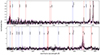 |
Fig. C.1. Composite spectrum of the newly identified AGN at z ∼ 3. The spectrum is obtained by combining the continuum-subtracted (0.15″ × 0.15″) spectra of the newly discovered type 2 AGN COS1656-B, COS1638-B, GS551-B, GS10578-B, Eastfield, and Mr West, by employing a bootstrap method (Perna et al. 2017b); before the combine, all spectra were normalised to the Hβ peak. Red vertical lines identify the main optical lines, while blue lines mark the position of coronal lines (CLs). No CLs are detected in the composite spectrum, but the most prominent emission lines show blue wings likely associated with outflows. |
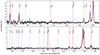 |
Fig. C.2. Composite spectrum of X-ray detected AGNs at z ∼ 3. The spectrum is obtained by combining the continuum-subtracted (0.15″ × 0.15″) spectra of the X-ray detected type 2 AGNs GS10578-A, COS1656-A, GS551-A, GS133, GS19293, GS20936, by employing a bootstrap method (Perna et al. 2017b); before the combine, all spectra were normalised to the Hβ peak. Red vertical lines identify the main optical lines, while blue lines mark the position of CLs. No CLs are detected in the composite spectrum. |
Appendix D: Horizon-AGN dual-AGN fraction predictions
The predicted dual AGN fractions reported in Fig. 14 were calculated using the following general rules. The parent population includes all systems with at least one AGN having luminosity above a given threshold. Each system is counted as a maximum of one pair, even if it has multiple AGNs. Therefore, for a population of ten systems, if one has ≥1 AGN companions, the dual AGN fraction is 1/10. This approach ensures a consistent calculation where each system is counted only once as a dual AGN, regardless of the number of active companions, and where the AGN population is a proxy for the number of massive galaxies undergoing galaxy mergers (e.g. Chen et al. 2023; Puerto-Sánchez et al. 2025).
We note that in Horizon-AGN, SMBHs are considered merged when their physical separation is less than 4 kpc. This could lead to an underestimation of the number of predicted dual and multiple AGN systems. Based on the distribution of physical distances in individual AGN systems, we estimated that the fractions in Fig. 14 could be underestimated by about ×5% for the sample with dp < 30 kpc and ×10 − 20% for the sample with dp < 10 kpc. Therefore, this effect should not be significant (see also Sect. 3.5 in Puerto-Sánchez et al. 2025). Additionally, we note that only one of our candidate dual AGN, GS551, has a projected separation of 2.9 kpc, which means its physical 3D separation could, in principle, be below 4 kpc.
All Tables
All Figures
|
Fig. 1. [O III] and Hα maps of the close environments of GA-NIFS AGN systems. They trace the emitting gas observed with NIRSpec IFS in the velocity channels v ∈ [ − 100, 100] km s−1 with respect to the AGN systemic redshift. Contours represent regions where the line emission reaches a significance level of 5σ. Each contour corresponds to emission from a specific velocity bin of 200 km s−1, spanning the full velocity range from −1100 to +1100 km s−1. Cyan contours indicate blueshifted gas, while orange contours mark redshifted gas. Cross symbols identify the AGN position in more complex (interacting) systems. All but GS3073 maps were obtained from NIRSpec cubes with 0.05″/pixel; for GS3073 we opted for the use of the finest 0.03″/pixel sampling to show the disturbed morphology due to very nearby companions (see also Fig. A.1 in Ji et al. 2024). All images are oriented north up, with east to the left. |
| In the text | |
|
Fig. 2. Lyα maps of the close environments of GS10578 (left) and GS551 (right). They trace the emitting gas with v ∈ [ − 200, 200] km s−1 observed with MUSE. The cyan (orange) contours indicate the Lyα emission at 4σ in velocity bins of 400 km s−1, from −1400 to +1400 km s−1. The cross symbols identify the (NIRSpec) AGN positions. The coordinate grids highlight the different rotation of MUSE data with respect to the standard north-east up-left configuration. |
| In the text | |
|
Fig. 3. [O III] map (top-left) and integrated spectra of the dual AGN system associated with COS1638. The [O III] map is obtained by integrating the [O III] emission over specific velocity ranges (as labelled), in order to highlight the primary (AGN-A) and secondary (AGN-B) nuclei, together with additional structures at the same redshift of the active galaxies. The panels on the right show the integrated spectra of the primary (top) and secondary (bottom) AGNs, extracted from the circular regions labelled in the map. The legend displays the individual Gaussian components and best-fit curves shown in the spectra; best-fit total profiles are represented in red for AGN-A and in blue for AGN-B. Residuals, defined as the difference between the observed data and the best-fit model, are displayed at the bottom of each panel; average ±3σ uncertainties on the data are also reported with horizontal grey shaded regions. The vertical blue and green shaded areas correspond to the velocity channels used to generate the [O III] map and contours in the top-left panel, respectively. Both targets present broad lines due to powerful outflows. |
| In the text | |
|
Fig. 4. [O III] map (top-right) and integrated spectra of the dual AGN system and a faint clump associated with COS1656. The [O III] map is obtained by integrating the [O III] emission over a velocity range from −200 to +200 km s−1, in order to highlight the primary (AGN-A) and secondary (AGN-B) nuclei; the contours trace the emission at v ∈ [ − 800, −600] associated with a clump close to AGN-B. The remaining panels show the integrated spectra of the primary (top-left) and secondary (bottom-left) AGNs, as well as of the clump (bottom-right), extracted from the circular regions labelled in the map. The legend display the individual Gaussian components and best-fit curves shown in the spectra; best-fit total profiles are represented in red for AGN-A, in blue for AGN-B, and in magenta for the clump. Residuals, defined as the difference between the observed data and the best-fit model, are displayed at the bottom of each panel; average ±3σ uncertainties on the data are also reported with grey shaded regions. The vertical green and blue shaded areas at ∼5007 Å mark the channels used to generate the [O III] map and contours in the top-right panel, respectively. |
| In the text | |
|
Fig. 5. [O III] map (top-right) and integrated spectra of the dual AGN system and a faint clump associated with Jekyll & Hyde. The [O III] map is obtained by integrating the line emission over specific velocity ranges (as labelled), in order to highlight the primary (Eastfield, AGN-A) and secondary (Mr West, AGN-B) nuclei, together with additional structures at the same redshift of the active galaxies. The remaining panels show the integrated spectra of the primary (top-left) and secondary (bottom-left) AGNs, as well as of a compact clump between the two brightest sources (bottom-right). The legend display the individual Gaussian components and best-fit curves shown in the spectra. Residuals, defined as the difference between the observed data and the best-fit model, are displayed at the bottom of each panel, with grey shaded regions indicating the average ±3σ uncertainties on the data. The vertical shaded areas at ∼5007 Å mark the channels used to generate the [O III] three-colour map. |
| In the text | |
|
Fig. 6. [O III] map (top-right) and integrated spectra of the dual AGN system and a faint clump associated with GS10578. The [O III] map is obtained by integrating the [O III] emission over a velocity range from −200 to +200 km s−1, in order to highlight the primary (AGN-A) and secondary (AGN-B) nuclei, together with additional structures at the same redshift of the active galaxies. The remaining panels show the integrated spectra of the primary (top-left) and secondary (bottom-left) AGNs, as well as of a compact clump between the two brightest sources (bottom-right). The legend display the individual Gaussian components and best-fit curves shown in the spectra. Residuals, defined as the difference between the observed data and the best-fit model, are displayed at the bottom of each panel, with grey shaded regions indicating the average ±3σ uncertainties on the data. The vertical green shaded area at ∼5007 Å mark the channels used to generate the [O III] map. |
| In the text | |
|
Fig. 7. [O III] map (top-right) and integrated spectra of the candidate dual AGN system associated with GS551. The [O III] map is obtained by integrating the [O III] emission over a specific velocity range (as labelled), in order to highlight the primary (AGN-A) and secondary (AGN-B) nuclei, together with additional structures at the same redshift of the active galaxies. The remaining panels show the integrated spectra of the primary (top-right) and secondary (bottom-right) AGNs. The legend display the individual Gaussian components and best-fit curves shown in the spectra; best-fit total profiles are represented in red for AGN-A, and in blue for AGN-B. Residuals, defined as the difference between the observed data and the best-fit model, are displayed at the bottom of each panel, with grey shaded regions indicating the average ±3σ uncertainties on the data. The vertical green shaded area at ∼5007 Å marks the channels used to generate the [O III] map, while the blue shaded area marks those associated with extended emission marked with contours overlapping the map. |
| In the text | |
|
Fig. 8. BPT diagram. Large red and blue circles refer to primary (AGN-A) and secondary (AGN-B) nuclei, respectively. All primary and secondary AGNs are above the solid (Kewley et al. 2001) and dashed (Kauffmann et al. 2003) curves, used to separate purely SFGs (below the curves) from galaxies containing AGNs (above the curves, i.e. the Seyfert region of the BPT). The olive curve indicates the locus of z ∼ 2.3 SFGs from (with intrinsic scatter relative to the median curve in light-olive Strom et al. 2017); additional measurements for z > 2.6 SFGs and AGNs are reported with small symbols (see legend and Sect. 6.1 for details). All reported measurements show that the Seyfert area of the BPT is free from contamination by SFGs at any considered redshift, and, therefore, ensure the AGN classification of the newly discovered sources COS1638-B, GS551-B, Eastfield, Mr. West, COS1656-B, and GS10578-B. All AGN-A and B flux ratios are reported in Table A.2. |
| In the text | |
|
Fig. 9. Comparison between Lyα (top) and [O III] emission maps (middle panels) for GS10578 (left) and GS551 (right), and spectra extracted from individual Lyα emitters (bottom). Both MUSE and NIRSpec images have been sampled with 0.05″/spaxel, to ease the comparison between UV and optical emission line spatial distributions. The Lyα maps are integrated over the emission profile at the location of the X-ray AGN, with overlaid contours indicating emissions at different wavelengths and highlighting nearby Lyα emitters. The bottom panels show spectra near the Lyα line for each system, in velocity space with respect to the systemic redshifts of the primary AGN; these spectra were extracted from regions with S/N > 5. In GS10578, two bright Lyα emitters (LAE1 and LAE2) are located ∼20 kpc south of the AGN; a Lyα halo at slightly lower redshift (z = 2.99) previously identified by Leclercq et al. (2017) is also marked with orange contours. GS551 features three Lyα emitters at varying distances up to ∼30 kpc; an even more distant Lyα emitter located ∼80 kpc to the north-east was also identified by den Brok et al. (2020, see their Fig. 2). The contours in the map panels are in steps of 1σ, for LAE_L17 and the GS551 companions, and in steps of 3σ (10σ) for GS10578 (GS551); all contours start from 5σ and are obtained integrating over the velocity channels shown in the bottom spectra according to their colours. These MUSE observations illustrate that GS551 and GS10578 are embedded in dense, complex environments. |
| In the text | |
|
Fig. 10. MUSE spectra of GS10578 (coral) and LAE2 (purple). These spectra were obtained by integrating over the regions at S/N > 4 in Fig. 9; for visual purposes, the LAE2 spectrum was shifted vertically, as labelled. The zoom-in insets show the same spectra in the vicinity of the lines used in the UV diagnostics used to classify LAE2 as an AGN (Fig. 12), together with 3σ errors for the LAE2 spectrum (grey area, mostly highlighting the position of strong sky line residuals). |
| In the text | |
|
Fig. 11. MUSE spectra of GS551 (coral), showing AGN-ionised lines, according to UV diagnostics (Fig. 12). These spectra were obtained by integrating over the regions at S/N > 4 in Fig. 2; for visual purposes, the LAE2 spectrum was shifted, as labelled. The zoom-in insets show the same spectra in the vicinity of the lines used in the UV diagnostics, together with 1σ errors for the LAE2 spectrum (green curve, mostly highlighting the position of strong sky line residuals). |
| In the text | |
|
Fig. 12. UV diagnostic diagram. Small green and red empty symbols represent model predictions for SFGs and AGNs, respectively, from Nakajima & Maiolino (2022). See the legend for details about model parameters. Large circles refer to the MUSE measurements of the three sources in our sample, as labelled; MUSE resolution does not allow us to separate the contribution of primary and secondary AGNs, but GS551 and GS10578 line ratios are likely dominated by the primary (brightest) AGN. The figure also shows individual X-ray AGNs (diamonds) and measurements from stacked AGN spectra (crosses), as well as SFGs at z ∼ 3 from the literature (green squares; see Sect. 5.2). GS551, GS10578 and LAE2 occupy the AGN region of the diagram. |
| In the text | |
|
Fig. 13. COS1638 X-ray emission. (a) Chandra image (obsID 15253) in the 0.5−7 keV observed-frame energy band, smoothed and sub-binned (1/2 pixel binning, i.e. 0.25″ pixel scale) for visualisation purposes. NIRSpec [O III] and X-ray contours are overlayed in black and in red, respectively. (b) radial profile of COS1638 in obsID 15253 extracted from the native-pixel event file, after masking the pixels affected by the PSF hook, using a set of 5 annuli (δr ≃ 0.5″) centred on the peak of the source emission (which corresponds to COS1638-A). The radial profile was fit with the radial PSF model (see Sect. 5.6) plus a constant set to the measured background level (model: PSF+constant). The red solid line shows the best fit, the blue dash-dotted line shows the simulated PSF profile, while the black dotted line shows the measured background level. The observed radial profile shows hints (∼2σ) of an X-ray excess at the distance of COS1638-B (∼2−3 native Chandra pixels, corresponding to ∼1.2″). (c) 0.5−7 keV images of the simulated PSFs at the positions of COS1638-A (marked with a ‘+’) and COS1638-B (‘x’). The lettered boxes show the extraction regions of the radial profiles in panel d. The magenta region shows the position of the hook feature, whose corresponding pixels were masked in the Chandra data before extracting the radial profiles. (d) 0.5−7 keV (observed energy range) radial profiles of COS1638 extracted from ObsID 15253, from masked (magenta) and unmasked (green) data. The black solid line marks the total X-ray profile obtained from fitting the data with the two PSFs (dash-dotted and blue dashed lines for COS1638-A and COS1638-B, respectively) and the background (grey dashed line). Thus, the X-ray morphology overall hints at the presence of a second peak at the position of COS1638-B. |
| In the text | |
|
Fig. 14. Dual AGN fraction as a function of redshift. The purple square shows the inferred dual AGN fraction from GA-NIFS observations, for the three newly discovered dual AGNs; instead, the violet symbol displays the fraction obtained also considering the two candidate dual AGNs; both measurements include 1σ Poisson errors for small numbers. The different curves represent the predicted AGN fractions obtained from an extension of the Volonteri et al. (2022) simulations up to z ∼ 6, passing different threshold criteria (as labelled). Notably, the figure shows that the GA-NIFS measurements moderately exceed the predictions obtained for thresholds that mimic our observational criteria, hence with projected distances dp < 10 kpc, log(Lbol, A) > 45 (for the primary AGN and the parent population) and log(Lbol, B) > 44 (for the secondary AGN), shown with a blue dashed curve (and Poissonian 1σ intervals in lightblue). The top panel shows the parent sample distributions of GA-NIFS sources (purple histogram) and simulated AGNs (blue for log(Lbol, A) > 45, grey for log(Lbol, A) > 43); we note that simulations at z > 5 suffer from poor statistics. |
| In the text | |
|
Fig. C.1. Composite spectrum of the newly identified AGN at z ∼ 3. The spectrum is obtained by combining the continuum-subtracted (0.15″ × 0.15″) spectra of the newly discovered type 2 AGN COS1656-B, COS1638-B, GS551-B, GS10578-B, Eastfield, and Mr West, by employing a bootstrap method (Perna et al. 2017b); before the combine, all spectra were normalised to the Hβ peak. Red vertical lines identify the main optical lines, while blue lines mark the position of coronal lines (CLs). No CLs are detected in the composite spectrum, but the most prominent emission lines show blue wings likely associated with outflows. |
| In the text | |
|
Fig. C.2. Composite spectrum of X-ray detected AGNs at z ∼ 3. The spectrum is obtained by combining the continuum-subtracted (0.15″ × 0.15″) spectra of the X-ray detected type 2 AGNs GS10578-A, COS1656-A, GS551-A, GS133, GS19293, GS20936, by employing a bootstrap method (Perna et al. 2017b); before the combine, all spectra were normalised to the Hβ peak. Red vertical lines identify the main optical lines, while blue lines mark the position of CLs. No CLs are detected in the composite spectrum. |
| In the text | |
Current usage metrics show cumulative count of Article Views (full-text article views including HTML views, PDF and ePub downloads, according to the available data) and Abstracts Views on Vision4Press platform.
Data correspond to usage on the plateform after 2015. The current usage metrics is available 48-96 hours after online publication and is updated daily on week days.
Initial download of the metrics may take a while.