| Issue |
A&A
Volume 692, December 2024
|
|
|---|---|---|
| Article Number | A171 | |
| Number of page(s) | 20 | |
| Section | Interstellar and circumstellar matter | |
| DOI | https://doi.org/10.1051/0004-6361/202451175 | |
| Published online | 12 December 2024 | |
Variability of the inner dead zone edge in 2D radiation hydrodynamic simulations
Max-Planck Institute for Astronomy (MPIA),
Königstuhl 17,
69117
Heidelberg,
Germany
★ Corresponding author; This email address is being protected from spambots. You need JavaScript enabled to view it.
Received:
19
June
2024
Accepted:
7
November
2024
Abstract
Context. The inner regions of protoplanetary discs are prone to thermal instability (TI), which can significantly impact the thermal and dynamical evolution of planet-forming regions. Observable as episodic accretion outbursts, such periodic disturbances shape the disc’s vertical and radial structure.
Aims. We have investigated the stability of the inner disc edge around a Class II T Tauri star and analysed the consequences of TI on the thermal and dynamic evolution in both the vertical and radial dimensions. A particular focus is laid on the emergence and destruction of solid-trapping pressure maxima.
Methods. We conducted 2D axisymmetric radiation hydrodynamic simulations of the inner disc in a radial range of 0.05 AU to 10 AU. The models include a highly turbulent inner region, the transition to the dead zone, heating by both stellar irradiation and viscous dissipation, vertical and radial radiative transport, and tracking of the dust-to-gas mass ratio at every location. The simulated time frames include both the TI phase and the quiescent phase between TI cycles. We tracked the TI on S-curves of thermal stability.
Results. Thermal instability can develop in discs with accretion rates of ≥3.6 ⋅ 10−9 M⊙ yr−1 and results from the activation of mag-netorotational instability (MRI) in the dead zone after the accumulation of material beyond the MRI transition. The TI creates an extensive MRI active region around the midplane and disrupts the stable pebble and migration trap at the inner edge of the dead zone. Our simulations consistently show the occurrence of TI reflares that, together with the initial TI, produce pressure maxima in the inner disc within 1 AU, possibly providing favourable conditions for streaming instability. During the TI phase, the dust content in the ignited regions adapts itself in order to create a new thermal equilibrium manifested in the upper branch of the S-curve. In these instances, we find a simple relation between the gas and dust-surface densities.
Conclusions. On a timescale of a few thousand years, TI regularly disrupts the radial and vertical structure of the disc within 1 AU. While several pressure maxima are created, stable migration traps are destroyed and reinstated after the TI phase. Our models provide a foundation for more detailed investigations into phenomena such as the short-term variability of accretion rates.
Key words: accretion, accretion disks / hydrodynamics / radiative transfer / protoplanetary disks / stars: protostars
© The Authors 2024
 Open Access article, published by EDP Sciences, under the terms of the Creative Commons Attribution License (https://creativecommons.org/licenses/by/4.0), which permits unrestricted use, distribution, and reproduction in any medium, provided the original work is properly cited.
This article is published in open access under the Subscribe to Open model.
Open Access funding provided by Max Planck Society.
1 Introduction
With the rising number of Earth-sized and super-Earth planets detected in close proximity to their stars, with orbital periods of around ten days (Mulders et al. 2015; Petigura et al. 2018; Mulders et al. 2018), questions about the conditions in the inner protoplanetary disc are gaining increasing relevance. Generally, the two pathways towards the existence of planets at such distances are the in situ formation via trapping and growing of inward-drifting pebbles (Chatterjee & Tan 2014; Jang et al. 2022) and the halting of planetary migration by a diminishment of the torques acting between the planet and the disc (Faure & Nelson 2016; Flock et al. 2019; Chrenko et al. 2022). For both of these processes, pressure maxima in the inner disc, capable of effectively trapping solid bodies, are required. A promising candidate for a mechanism creating such bumps in the pressure profile within ~1 AU of the host star is the transition between a hot inner disc in which temperatures and ionisation levels are sufficiently high to allow for the emergence of magnetorotational instability (MRI, Balbus & Hawley 1991) and a cold outer disc where the levels of turbulence are significantly smaller (e.g. Dzyurkevich et al. 2013; Cui & Bai 2022). In the context of two-dimensional axisymmetric simulations, Flock et al. (2016) and Flock et al. (2019) have shown that this transition lies at distances between 0.1 and 1 AU, depending on the stellar luminosity, and indeed provides favourable conditions for halting both the pebble drift and the migration of planets. However, their models represent the radiation-hydrostatic structure of the inner disc without considering dynamic effects and heating by viscous dissipation.
Several studies indicate that the structure of the inner disc is not stable over long periods of time but undergoes phases of variation induced by thermal instability (TI) in the inner regions of the dead zone (Lin et al. 1985; Kley et al. 1999; Wunsch et al. 2005; Zhu et al. 2010; Martin & Lubow 2011; Faure et al. 2014). These regions are considered thermally unstable if a small temperature perturbation causes a significant increase in the heating rate compared to the cooling rate, leading to runaway heating (Armitage 2019). There are two scenarios of interest whereby this condition can be met in the inner regions of protoplanetary discs. The first scenario occurs when gas opacity increases sharply with temperature due to the ionisation of hydrogen at temperatures of ~104 K, reducing the cooling rate and trapping heat near the midplane, (commonly referred to as ‘classical’ TI, Bell & Lin 1994; Zhu et al. 2009b). In the second scenario, viscosity increases significantly with temperature due to the activation of the MRI at temperatures of around 1000 K, greatly enhancing the heating rate (Desch & Turner 2015; Zhu et al. 2009a; Steiner et al. 2021). If either or both of these scenarios occur, the corresponding region of the disc is considered thermally unstable (Armitage 2019).
Such instabilities are also indicated in investigations of the thermal structure of the inner disc, which often result in multiple solutions for the vertical thermal balance when the influence of viscous dissipation and the strong temperature dependence of the gas opacity are considered (Jankovic et al. 2021; Pavlyuchenkov et al. 2023). This results in the typical ‘S-curves’ of thermal stability in the Σ–Teff plane, where Σ is the surface density and Teff is the effective temperature at a fixed radius (e.g. Martin & Lubow 2011; Nayakshin et al. 2024). In this context, the TI constitutes the switch of the respective disc region from the stable lower branch of the S-curve to the stable upper branch. Such a description is analogous to the effects of the well-known disc instability model for cataclysmic variables such as dwarf novae or X-ray transients (DIM; see, e.g. the review by Hameury 2020). The TI is induced as soon as the surface density reaches a critical value, after which a heating front is launched into the dead zone of the disc in a ‘snowplough’ fashion (Lin et al. 1985). The sudden increase in turbulence in the massive dead zone results in a strong elevation of the accretion rate onto the central star. This is why TI in the inner disc is one of the candidates for physical processes that may be able to explain observed episodic accretion bursts in young stellar objects such as FU Ori (Herbig 1977; Kley et al. 1999; Audard et al. 2014).
While a few 2D axisymmetric models of the TI of the inner disc exist (Kley et al. 1999; Zhu et al. 2009b), most theoretical studies of TI-induced episodic accretion events do not resolve the vertical structure of the inner disc (e.g. Zhu et al. 2010; Bae et al. 2013, 2014; Macfarlane et al. 2019; Kadam et al. 2022; Cleaver et al. 2023). Moreover, these investigations were tailored to explain the timescale and magnitudes of massive accretion outbursts of Class 0/I young stellar objects. In such young massive discs, the activation of the TI mainly relies on the inward transport of material by gravitational instability (GI) (e.g. Vorobyov & Basu 2006). However, both theoretical models and observations have shown that less massive Class II objects are prone to TI as well (Kóspál et al. 2016; Steiner et al. 2021; Chambers 2024). In these objects, GI does not play a dominant role, and material is piled up in the inner regions of the dead zone by hydrodynamic instabilities (e.g. Lyra & Umurhan 2019; Cui & Bai 2022) until the critical surface density for MRI activation is reached and the TI is initiated.
Simple 1D models by Chambers (2024) indicate that the heating fronts launched by the TI create pressure maxima in the radial disc structure within 1 AU, which could serve as traps for drifting pebbles. The silicate sublimation front (e.g. Kama et al. 2009) plays an important role in the initiation and development of the TI because the associated strong change in opacity constitutes a respective change in disc temperature by absorbing the bulk of the stellar irradiation (Flock et al. 2016, 2019). Therefore, at least in passively heated discs, the location of the MRI transition and the location of the inner dust rim are closely related. Schobert et al. (2019) show that the additional consideration of heating by viscous dissipation can shift the inner edge of the dead zone further outwards, while leaving the location of the dust sublimation front mostly unchanged for large accretion rates. However, analogously to Flock et al. (2019), the models of Schobert et al. (2019) simulate the hydrostatic structure of the inner disc and do not consider the implications for dynamical evolution.
Instead of focussing a priori on the recreation of observed luminosity features of outbursting T Tauri stars, this work aims to analyse the inner disc’s stability and the consequences of potential TI-induced accretion events on the vertical and radial structure and evolution of a disc around a Class II T Tauri star. In our models, the TI is induced by the activation of the MRI in the dead zone. The ‘classical’ TI caused by hydrogen ionisation and the consequent strong temperature dependence of the opacity does not occur in our simulations. In contrast to previous works investigating the hydrodynamic evolution, our models include a permanently MRI active inner disc and the transition to the dead zone within the computational domain. Furthermore, we include heating by both stellar irradiation and viscous dissipation, radiation transport in the radial and vertical direction, and tracking of the variable dust-to-gas mass ratio throughout the inner 10 AU of the disc. This allows us to also monitor the evolution of the dust sublimation region during the TI phase. We take the hydrostatic model of the inner disc rim around a T Tauri star by Flock et al. (2019) as an initial model and evolve it in time under the influence of viscous heating.
The paper is organised as follows. In Sect. 2, we describe the numerical and physical set-up of our model, including the equations and parameters governing both the initial configuration and the time-dependent evolution. In Sect. 3, the results of our simulations are presented and consecutively analysed and discussed in Sect. 4. Finally, we summarise the main conclusions in Sect. 5.
2 Method
The simulations conducted in this work consist of two parts. First, an initial model was created by finding a solution for the hydrostatic equilibrium, including irradiation by the central star, dust sublimation, and a simplified description of viscous heating. The creation of this model is elaborated on in Sect. 2.1. Second, the hydrostatic solution was used as a starting configuration for the time-dependent radiation hydrodynamic simulation, which is described in Sect. 2.2. For both steps, we used the finite volume method of the PLUTO Code (Mignone et al. 2007). In Sect. 2.3, we describe the implementation of turbulent viscosity in our model, while Sects. 2.4 and 2.5 contain the description of dust sublimation and utilised opacities, respectively. Finally, in Sect. 2.6, we give a brief overview of the numerical set-up of the simulated domain together with the implemented boundary conditions.
2.1 Initial model
The construction of the hydrostatic initial model generally followed the description in Flock et al. (2019) with the addition of the effect of viscous heat dissipation. After building an initial surface density profile, depending on the viscosity, ν, and a chosen radially constant mass flux, Ṁinit, according to
 (1)
(1)
and determining an initial temperature field, T(r, θ), utilising the optically thin solution, we solved the equations of hydrostatic equilibrium in spherical co-ordinates (r, θ, ϕ) assuming axisym-metry. The solution provides a density- and azimuthal velocity field, ρ(r, θ) and vϕ(r, θ). Using the equation of state of an ideal gas,
 (2)
(2)
to couple the thermal pressure, P, with the temperature, T, where kB is the Boltzmann constant, µg is the mean molecular weight, and u is the atomic mass unit, in conjunction with ρ(r, θ) we established radiative equilibrium by finding a steady-state solution of the system of two coupled radiative transfer equations,
 (3)
(3)
 (4)
(4)
The equations above describe the heating, cooling, and radiative diffusion in the flux-limited approximation, where γ is the adiabatic index, κP and κR are the Planck and Rosseland mean opacities, respectively, aR = 4 σB/c is the radiation constant (with σB being the Stefan-Boltzmann-constant and c being the speed of light), ER is the radiation energy, and λ is the flux limiter function (Levermore & Pomraning 1981). We assumed a blackbody irradiation flux, F*, which can be evaluated at every radius by
 (5)
(5)
considering the effect of the radial optical depth, τ* (which is described in Sect. 2.4). R* and T* are the stellar radius and the stellar surface temperature, for which we adopted the values of R*. = 2.6 R⊙ and T* = 4300 K, respectively, following the model set-up of Flock et al. (2019).
Qacc describes the heating by viscous dissipation. Its implementation followed the procedure described in Schobert et al. (2019). In hydrostatic equilibrium, it can be assumed that the dominant contribution to the velocity field is υϕ. Therefore, the viscous heating term in spherical co-ordinates takes the simplified form
![Mathematical equation: ${Q_{{\rm{acc}}}} = \mu {\left[ {r{\partial \over {\partial r}}\left( {{{{\upsilon _\phi }} \over r}} \right)} \right]^2} = \mu {\left[ {r{{\partial \Omega } \over {\partial r}}} \right]^2},$](/articles/aa/full_html/2024/12/aa51175-24/aa51175-24-eq6.png) (6)
(6)
with the orbital frequency, Ω, and dynamic viscosity, µ, as the product of the local density, ρ, and the kinematic viscosity, ν,
 (7)
(7)
For the kinematic viscosity, we used the description introduced by Shakura & Sunyaev (1973) with the stress-to-pressure ratio, α, and the local speed of sound, cs.
We note that if viscous heating and dust evaporation are considered and the mass accretion rate is high enough to enable significant heating by viscous dissipation, TI is expected in the inner disc (Pavlyuchenkov et al. 2023). This impedes the convergence of our computational method to find a hydrostatic solution for the initial model, which has also been recognised by Schobert et al. (2019). This is why α was kept at a fixed value of 10−3 in the viscous heating term in Eq. (3) (similar to Schobert et al. 2019) during the creation of the initial model. To determine the initial surface density distribution (Eq. (1)) and during the hydro-dynamic simulation, α was adapted according to the description given in Sect. 2.3.
The initial mass in the computational domain of our simulations was controlled by the radially constant mass flux, Ṁinit. Consequently, this also influences the pile-up of mass at the inner dead zone edge, and therefore the effectiveness of viscous heating and heat-trapping, which potentially leads to the onset of the TI-induced accretion event. Furthermore, if an accretion event occurs, Ṁinit determines the available mass to be accreted and consequently has a significant influence on the duration and peak accretion rate of the burst. In this work, we implemented four values for Ṁinit ranging from 3.6 ⋅ 10−10 M⊙ yr−1 to 1 ⋅ 10−8 M⊙ yr−1, which is consistent with observed values in the young (≤ 1 Myr) star cluster NGC 1333 (Fiorellino et al. 2021) as well as in the older star-forming regions Lupus (Alcalá et al. 2017) and Chameleon I (Manara et al. 2017).
2.2 Time-dependent simulation
For the time-dependent simulation, we solved the following set of radiation-hydrodynamic equations:
 (8)
(8)
 (9)
(9)
![Mathematical equation: $\eqalign{ & {{\partial E} \over {\partial t}} + \nabla \cdot \left[ {\left( {E + {P_{{\rm{gas}}}}} \right)\upsilon } \right] = - \rho \,\upsilon \cdot \nabla \Phi - {\bf{\Pi }}:\nabla \upsilon \cr & \,\,\,\,\,\,\,\,\,\,\,\,\,\,\,\,\,\,\,\,\,\,\,\,\,\,\,\,\,\,\,\,\,\,\,\,\,\,\,\,\,\,\,\,\,\,\,\,\,\,\,\,\,\, - {\kappa _{\rm{P}}}\rho \,c\left( {{a_{\rm{R}}}{T^4} - {E_{\rm{R}}}} \right) - \nabla \cdot {F_*}, \cr} $](/articles/aa/full_html/2024/12/aa51175-24/aa51175-24-eq10.png) (10)
(10)
with the velocity vector, υ = (υr, υθ, υϕ), the gas pressure, Pgas, the total energy, E, and the gravitational potential, Φ = GM*/r, where G is the gravitational constant and M* is the mass of the star, which we fixed at M* = 1 M⊙ for this work. Π represents the viscous stress tensor, describing the viscous angular momentum transport in the equations of motion (Eq. (9)) and viscous heating in the energy equation (Eq. (10)) in the respective terms. ∇υ (an abbreviation of ∇ ⊗υ where ‘⊗’ is the dyadic product) is the velocity gradient tensor. Utilising the identity A : (b ⊗ c) = b ⋅ (A ⋅ c), where A is a tensor and b and c are vectors, the viscous heating term in Eq. (10) can also be written as
 (11)
(11)
with the stress tensor taking the form
![Mathematical equation: ${\bf{\Pi }} = \mu \left[ {\nabla \upsilon + {{(\nabla \upsilon )}^{\rm{T}}} - {2 \over 3}(\nabla \cdot \upsilon ){\bf{I}}} \right].$](/articles/aa/full_html/2024/12/aa51175-24/aa51175-24-eq12.png) (12)
(12)
I denotes the unit tensor. If the contributions of the radial and polar components of the velocity can be neglected, Eq. (11) results in the expression for Qacc (Eq. (6)).
As a closure relation, we again used the ideal gas equation. After finding a solution to the system of Eqs. (8), (9), and (10), the coupled equations for the radiation transport, Eqs. (3) and (4), were solved to acquire the temperature and the radiation energy for the next time step. Since the heating by viscous dissipation was already accounted for by the corresponding term in the total energy equation (where the contributions from the radial and polar velocity gradients are considered as well), we omitted the viscous heating term, Qacc, in Eq. (3) during the time-dependent simulation.
2.3 Viscosity
The stress-to-pressure ratio entering the viscous stress description can adopt two different values, αMRI or αDZ, depending on the local temperature. αMRI was implemented if the temperature of the environment was high enough to sustain MRI, while αDZ was used at lower temperatures (in the dead zone). To ensure a smooth transition between these values around a critical temperature, TMRI, the stress-to-pressure ratio takes the form
![Mathematical equation: $\alpha = \left( {{\alpha _{{\rm{MRI}}}} - {\alpha _{{\rm{DZ}}}}{1 \over 2}\left[ {1 - \tanh \left( {{{{T_{{\rm{MRI}}}} - T} \over {25{\rm{K}}}}} \right)} \right] + {\alpha _{{\rm{DZ}}}}.} \right.$](/articles/aa/full_html/2024/12/aa51175-24/aa51175-24-eq13.png) (13)
(13)
In our simulations, αMRI was set to a value of 0.1. This is motivated by the findings of Flock et al. (2017b), who argue that the stress-to-pressure ratio can be as high as 10% in the MRI active zone if a net vertical flux is present. Furthermore, models with αMRI = 0.1 have been shown to be consistent with observed signatures of YSOs undergoing accretion burst events (e.g. Cleaver et al. 2023; Liu et al. 2022). The residual viscosity in the dead zone αDZ was chosen to be 10−3, which represents hydrodynamic turbulence (e.g. Lyra & Umurhan 2019; Cui & Bai 2022). This value also ensures that the surface density in the computational domain is small enough to keep the Toomre parameter (Toomre 1964) well above 1. Therefore, we did not consider the effects of GI in our simulations. In accordance with Flock et al. (2019), we assumed the MRI activation temperature, TMRI, to be 900 K.
2.4 Dust sublimation
Following Flock et al. (2016) and Flock et al. (2019), we used the following fitted function for the evaluation of the dust sublimation temperature (Isella & Natta 2005),
 (14)
(14)
which then allowed us to determine the dust-to-gas mass ratio,
![Mathematical equation: ${f_{{\rm{D}}2{\rm{G}}}} = \{ \matrix{ {{f_{\Delta \tau }}{1 \over 4}\left[ {1 - \tanh \left( {{{\left( {{{T - {T_{\rm{S}}}} \over {150{\rm{K}}}}} \right)}^3}} \right)} \right]\left[ {1 - \tanh \left( {2/3 - {\tau _*}} \right)} \right]} \hfill \cr {{f_0}{\rm{for}}T\left\langle {{T_{\rm{S}}}{\rm{and}}{\tau _*}} \right\rangle 3.0} \hfill \cr } .$](/articles/aa/full_html/2024/12/aa51175-24/aa51175-24-eq15.png) (15)
(15)
Within this description, f∆τ represents the respective dust-to-gas mass ratio that results in an optical depth of ∆τ = 0.2 in a computational grid cell. It takes the form f∆τ = 0.2/[ρ κP(T*) ∆r] − κgas/κP(T*), where κP(T*) is the dust opacity resulting from averaging the wavelength-dependent opacity over the spectrum of the light from the star irradiating the disc, κgas is the gas opacity, and ∆r is the radial extent of the grid cell. This formulation of f∆τ ensures that the absorption of radiation by a single cell is limited, allowing us to properly resolve the absorption at the inner edge of the dust disc. Equation (15) describes a smooth transition of the dust-to-gas ratio between a minimum value of 10−10 (which was set to facilitate numerical stability) and the maximum value of f0 around the sublimation temperature1 and around the area where a radial optical depth of τ* = 2/3 is reached, which is where most of the stellar irradiation is absorbed. In this context, the radial optical depth was calculated as
 (16)
(16)
with  being the optical depth at the inner radius of the computational domain r0, assuming that the dust-to-gas ratio in the disc between r0 and the stellar surface is zero. σ* was given by the sum of the contributions to the optical depth from dust and gas, σ* = ρdust κP(T*) + ρgas κgas .If τ* > 3.0 and the temperature of the disc material is smaller than the local sublimation temperature, we set the dust-to-gas ratio to its maximum value f0. We adopted f0 = 10−3 to account for the part of the dust content that contributes to the opacity used in the radiative transfer scheme and is well coupled to the gas. This value does not include grown dust already settled towards the mid-plane, which does not play a significant role in determining the infrared opacity.
2.5 Opacities
As is described in Flock et al. (2019), κgas was taken as an average of Rosseland mean opacities calculated by Malygin et al. (2014). The average was calculated for the parameter space relevant to our models. Flock et al. (2019) derived an average value of κgas = 10−5 cm2 g−1 for the conditions of the gas phase in the hydrostatic case. The same value has been adopted here for the creation of the initial model. During the hydrodynamic simulation, we recalculated the mean value for the gas opacity to account for the increased temperature, density, and pressure of the gas disc during phases of TI. By considering this adapted parameter space, we derived a value of κgas = 10−3 cm2 g−1 for the Rosseland mean gas opacity (see Appendix A). Following Flock et al. (2019), we assumed the same value for the irradiation opacity. With this increase in gas opacity, optically extremely thin regions could be avoided. Such regions are unable to cool efficiently, which leads to strong temperature increases when heating mechanisms (in addition to irradiation heating) in the time-dependent simulations are considered. As a consequence, the numerical stability of the hydrodynamic simulations is significantly enhanced. For the dust opacities, we assumed κP = κR and adopted the two values derived by Flock et al. (2019): the irradiation opacity corresponding to the stellar surface temperature, κP(T*) = 1300 cm2 g−1, and the thermal emission opacity corresponding to a typical dust sublimation front temperature of ĸP(1500K) = 700 cm2 g−1.
2.6 Numerical domain configuration and boundary conditions
The set-up of the computational domain was the same as in Flock et al. (2019). The simulations incorporated the inner part of a protoplanetary disc in spherical co-ordinates with the radial extent ranging from rin = 0.05 AU to rout = 10 AU and the meridional extent being symmetric around the disc midplane with θ = π/2 ± 0.15. The numerical grid consisted of Nr = 2048 logarithmically spaced grid points in the radial direction and Nθ = 128 linearly spaced points in the meridional direction.
We imposed Neumann (zero gradient) conditions at the radial inner (rin) and outer (rout) boundary for the radial and poloidal velocity. A linear extrapolation was used for the azimuthal velocity and the density to facilitate the continuation of the gradients of the respective quantities. At the upper and lower poloidal boundaries, the continuation of the density gradient was implemented as well while using free Neumann conditions for all velocity components.
An inflow of mass into the computational domain was unde-sired for our models. Therefore, if the zero gradient condition would allow for an inflow (i.e. if the velocity in the cells next to the boundary is pointing into the domain), the velocities were reflected in the boundary2. Although we calculated the conditions in the disc beyond ~2 AU in the same manner as in the inner disc, for the purpose of our simulations, these regions technically act as a mass reservoir for refilling the inner disc after it has been depleted by the TI-induced accretion event. Since the viscous timescale at the outer boundary (10 AU) is of the order of 106 yr, which is much larger than the time frame simulated by our models, the chosen no-inflow condition at the outer radial boundary should not affect our results. Furthermore, global disc models have shown that TI-induced accretion events can still occur when the inner disc is cut off from resupply of material from radii greater than 10 AU by, for example, gaps in the disc structure (Cecil et al. 2024).
A zero gradient condition was used for the temperature at all four boundaries. The radiation energy density at the boundaries was determined by ER(∂U) = σ[T0(∂U)]4 where ∂U is the boundary of the domain. Hereby, T0 is the temperature of a disc region that is optically thin with respect to the irradiation of starlight and is calculated as
 (17)
(17)
which was also used as an initial temperature field for creating the hydrostatic initial model. ϵ is the ratio between the absorption and emission efficiencies, which simplifies in this case to the ratio of irradiation opacity, κP(T*), to thermal emission opacity, κP(TS), when neglecting the contribution of the gas opacity (e.g. Ueda et al. 2017). The factor 1/2 was included to allow for efficient cooling of the disc by radiation3.
Implemented parameters for the reference monospace MREF.
3 Results
The purpose of this work is to analyse the temporal behaviour of the inner parts of a protoplanetary disc under the influence of stellar irradiation, radial and vertical radiative transfer, dust sublimation, turbulent α-parameterised activity, and viscous heating. For that purpose, we constructed a reference model, MREF, the parameters of which are summarised in Table 1. Several additional models were set up to investigate the influence of different initial accretion rates and, consequently, different inner disc masses. An overview of the chosen parameters and names for the different models is given in Table 2.
Initial accretion rates for the different models analysed in this work.
3.1 Initial configuration
Panels a and c of Fig. 1 show the temperature and gas density map of the initial configuration of the reference model MREF. The structure of the disc is similar to the one described in Flock et al. (2016), Flock et al. (2019) and Schobert et al. (2019): a pure gas disc is present at radii smaller than 0.09 AU, followed by an arched inner dust rim between 0.09 AU and 0.15 AU. The transition from an MRI active inner disc to the dead zone occurs at a radius of 0.15 AU in the midplane. The transition region stays at a constant radius in the vertical direction until it crosses the τ* = 2/3 line, after which the medium in the line of sight towards the star is optically thin, and the MRI transition moves outwards. After a shadowed region between ~0.15 AU and ~0.25 AU, a flared disc extends towards rout. At radii between 0.15 AU and 0.2 AU, which is the region where the MRI transition takes place, multiple vertical ripples are visible in the temperature and density distribution. These disturbances are an indication of TI. The conditions in the initial configuration of the MREF model are such that viscous heating and heat-trapping around the disc midplane shortly beyond the MRI transition are effective enough to elevate the temperature to values at which the viscous α parameter becomes dependent on the temperature (according to Eq. (13)). However, the development of the TI is suppressed by the computational method, which aims to find a hydrostatic solution. In fact, we found multiple solutions for the hydrostatic structure, between which the solving algorithm switches after every iteration. This finding is similar to the conclusion of Pavlyuchenkov et al. (2023), who find that there is no unique solution to the thermal structure when considering accretion heating, dust evaporation, effects of gas opacity, and a sufficiently high accretion rate. In the context of S-curves of thermal balance, this means that the surface density adopts values that allow for at least two temperature values, all of which would result in a vertical thermal equilibrium. However, we find that the choice of the initial model between these different configurations is irrelevant to the evolution of the disc during the hydrodynamic simulation. Although the stress-to-pressure ratio, α, was kept constant in the calculation of the viscous heating term for the hydrostatic equilibrium, the surface density was determined according to Eq. (1) with the contribution of an adaptive α, as it is described in Eq. (13). A change in temperature in the vicinity of TMRI due to viscous heating translates to a change in α and consequently to an alteration of Σ. Therefore, the non-existence of a unique solution for the thermal structure manifests itself in the form of jumps in Σ, leading to the ripples visible in panels a and c of Fig. 1. During the hydrodynamic simulation, these ripples are smoothed out and the disc adopts the structure visible in panels b and d of Fig. 1 unless a TI is in progress (which is analysed in Sect. 3.2). Figure 2 shows the surface density distributions of the models listed in Table 2 at various stages during their evolution. The profiles depicted in panel a represent the initial configuration (at t = t0). The unstable region of MREF (blue line) is discernible here as well by the jumps in Σ due to the aforementioned reasons. In the model M3 with a higher initial accretion rate, this unstable behaviour is magnified due to the increased viscous heating caused by a larger density in the dead zone. While the ripples in the surface density of M2 are less severe, they are almost completely absent in M1 because the viscous heat dissipation and heat-trapping close to the midplane are less effective in these less massive discs.
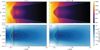 |
Fig. 1 Temperature (panels a and b) and gas density (panels c and d) maps for the model MREF in the initial configuration at t = t0 and at the end of the quiescent phase, shortly before the TI is triggered, t = tTI − ∆t. Yellow contour lines depict the region of dust sublimation (T = Ts), black lines show the ionisation transition from the MRI active zone to the dead zone (T = TMRI), and green lines mark the radial optical depth τ, = 2/3 surface. In panels c and d, the red contours are drawn at ρgas = 10−9 which corresponds to a dust density of ρdust = 10−12. |
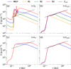 |
Fig. 2 Surface density profiles of models with different Ṁint at distinct evolutionary stages. Panel a shows the initial configuration for all models, while panel b presents their structure after the first TI and the subsequent diffusion of the resulting density bumps. Panel c compares the surface density of MREF and M3 at the start of their respective second TI cycle, and panel d shows the structure of both models after they have become quiescent again (similar to panel b). In all cases, the TI phase persists until enough mass has been accreted so that the surface density does not exceed Σcut. |
3.2 Thermal instability phase
After starting the hydrodynamic simulation, MREF as well as M2 and M3 immediately enter the TI stage, which is expected since the initial models already show signs of instability. We acknowledge that this first dynamic instability phase may be strongly influenced by our choice of the hydrostatic initial configuration and the transition of the gas opacity from 10−5 cm2 g−1 in the hydrostatic case to 10−3 cm2 g−1 in the hydrodynamic case. Therefore, we refrained from conducting a detailed analysis of the initial TI cycles. Model M1 does not show the development of TI since the density is small enough so that the combination of a low level of viscous heat dissipation and the small vertical optical depth does not lead to efficient heat-trapping inside the disc.
The models’ surface densities after the initial burst (at a time denoted as tcut1) are shown in panel b of Fig. 2. We find that in all cases the amount of material accreted onto the star is such that the surface density after the TI phase smoothes out into a structure that does not exceed a characteristic profile Σcut ∝ r0.8137. In panel a of Fig. 2, Σcut is plotted over the surface densities in the initial configuration. Notably, all models with surface densities larger than Σcut enter the outbursting stage. The small amount of mass that causes the surface density of M1 to barely rise above Σcut around 0.15 AU is rapidly accreted onto the star without similar TI properties compared to the other models.
The models MREF and M3 enter another TI-induced outburst-ing phase at a time referred to as tTI. The surface densities of those two models at their respective t = tTI are shown in panel c of Fig. 2. Σcut is depicted again as a reference. The comparison to panel b makes clear that the density maximum present shortly before and shortly beyond 1 AU, respectively, after the initial instability (at t = tcut1 ), has smoothed out during the quiescent phase between the TI cycles and mass has been accreted towards the star, increasing the surface density above Σcut again. The mass tends to accumulate at the inner edge of the dead zone due to the large amount of angular momentum transported outwards from the highly viscous, MRI active inner disc. As soon as enough material has accumulated so that viscous heating near the midplane is effective enough and the vertical optical depth from the midplane towards the disc surface is large enough to trap the heat and increase the midplane temperature towards values in the vicinity of TMRI , the TI develops and the disc enters the outbursting stage. The mass accumulation during the quiescent phase in the models M1 and M2 is insufficient for triggering a TI cycle. Panel d of Fig. 2 shows the surface density profiles of MREF and M3 after their respective second TI phases (at t = tcut2). Analogously to the disc structures shown in panel b, enough mass has been accreted so that the surface density does not exceed Σcut.
Panels a and b of Fig. 3 show the evolution of the accretion rate onto the star, Ṁ, and of the radius of the inner edge of the dead zone at the midplane, rDZ, over a time frame of 3000 yr for the models with varying initial accretion rates. After the initial bursts at the start of the simulations (in all models except for M1), the discs enter a quiescent stage in which the inner disc is resupplied with material accreted from larger radii. The second TI cycles occurring in the models MREF and M3 are initiated at times of 2522 yr and 2350 yr, respectively, after the start of the hydrodynamic simulation. The thermal- and density structure of MREF at the beginning of this phase (shortly before the TI is triggered, denoted with t = tTI − ∆t) is depicted in panels b and d of Fig. 1. The shape of the inner rim is similar to the one of the initial model described in Sect. 3.1 with the notable differences that the disc is thinner and stretches further towards the star. Furthermore, the disc in panels b and d is the solution to the full set of radiation hydrodynamic equations, which means that potential ripples in the density structure are either smoothed out or lead to a runaway TI in contrast to the hydrostatic case shown in panels a and c. The state of the disc in the quiescent phase and just before the onset of the TI is very similar to the structure of the inner disc shown in Fig. 1 of Flock et al. (2019). The viscous heating effect in our model manifests in the slightly larger contrast between the midplane temperature and the temperatures between the midplane and the τ* = 2/3 surface.
Panels a1 and b1 of Fig. 3 are a zoom-in to the temporal evolution of the mass accretion rate and radius of the dead zone inner edge at the midplane, respectively, for the model MREF during the burst. The accretion event consists of multiple reflares, which decrease in amplitude with time. The vertical dashed lines in panels a1 and b1 indicate points in time, which are used to analyse the reflare mechanism in Sect. 3.4.
Table 3 summarises several properties of the outbursts occurring in MREF and M3. We define the total duration of the burst tburst as the time between the start of the rapid rise of the accretion rate and the point in time at which the accretion rate has decreased back to the pre-burst value. During this time frame, a maximum accretion rate of Ṁmax is reached, which corresponds to an amplification of a factor, ƒamp, with respect to the accretion rate just before the TI sets in. A total mass of Macc is accreted onto the star over the course of an outburst and the inner edge of the dead zone at the midplane travels to a maximum distance of rDz,max. The comparison with the values extracted from the accretion event in M3 shows that all these quantities are universally increased in a more massive disc.
Snapshots of the temperature structure and corresponding surface density at certain times during the burst in MREF are shown in Fig. 4. At t = tTI (first column, corresponding to the stage of the disc shown in panel c of Fig. 2), the temperature in the dead zone is raised above TMRI first at the midplane at a radius of 0.135 AU, which is slightly outside rDZ, which is located at 0.10 AU. The radial profile of the midplane temperature at t = tTI for MREF is depicted as the dashed blue line in Fig. 5 in comparison with the more massive M3 model. In both models, the instability is ignited at the same position, which is a consequence of rDZ being the same in both cases during the quiescent phase (panel b of Fig. 3). The rise in α caused by the temperature increase leads to more rigorous viscous dissipation, letting the temperature build up rapidly further towards the dust evaporation temperature, TS, at the point of first ignition. The material in the surrounding area is quickly heated up and becomes MRI active as well. This launches an ionisation front in all directions, promptly reaching the inner, permanently MRI active gas disc. The ionisation (or heating) front is characterised as the moving boundary between the MRI active and inactive regions when it propagates into the dead zone. In MREF, the freshly ignited MRI active zone reaches z/r=±0.06 within a time of about one month and continues to expand vertically as the ionisation front travels outwards. After about 8 yr, the MRI active zone has reached its maximum extent, with a radius of 0.6 AU at the midplane and a vertical reach of up to z/r=±0.08 at 0.3 AU, which corresponds to 0.02 AU (or roughly two scale heights) above and below the midplane. The time at which this stage is reached is denoted with tc. The disc’s temperature map and surface density structure at that time are shown in the second column of Fig. 4. The yellow contour line indicates that the temperature within the ignited zone increases towards TS, which constitutes an equilibrium temperature.
The solid blue line in Fig. 5 shows the midplane temperature of MREF at t = tc. Only in the very inner parts at radii smaller than 0.1 AU does the midplane temperature increase slightly above TS due to the large density of the accreted accumulated material and consequently significant viscous heat dissipation. The comparison with the profile of M3 at t = tc (solid red line) shows that in the more massive model, the ionisation front is able to travel farther and a larger part of the dead zone becomes MRI active. Hence, more mass is being accreted and the enhanced density of the accreting material in the inner disc allows the temperature to rise significantly above TS. Notably, even when the TI is fully developed, there is still a thin dust arc between the ignited, viscously heated area and the inner gas disc. This arc is pushed close to the star, towards a radius of 0.055 AU in the case of MREF. It is manifested as a temperature sink close to the star, visible in the solid blue line in Fig. 5. The arc constitutes the inner dust rim, as explored in Flock et al. (2019), which we resolve numerically using our description for the dust-to-gas ratio (Eq. (15)). The rim travels closer to the star due to the large increase in density in the inner disc by the accretion process during the burst. In addition to f∆τ and the resolution of the simulation, the thickness of the arc depends on the choice of the value of τ* above which fD2G is set to its maximum value f0. In our models, this threshold value is set to 3.0. A larger value would lead to a thicker arc separating the inner gas disc from the ignited area since the increase in optical depth per unit length is limited by f∆τ for larger radii compared to a smaller value. This limiting mechanism leads to a larger optically thin region beyond the dust sublimation front, which enables more efficient cooling and, therefore, increases the extent of the area where dust can exist. As soon as the τ* threshold is reached, the dust-to-gas mass ratio increases quickly, creating an optically thick disc that is able to trap the viscously created heat and the temperature increases above TS again. Although this arc is capable of blocking stellar irradiation, its existence and thickness do not change the thermal and dynamical evolution of the inner disc, since the heating is dominated by viscous dissipation during the TI phase. We utilised this description of fD2G in most of our simulations to be able to resolve the inner dust rim and stay consistent with the models of Flock et al. (2019). However, we also created an alternative prescription, which is more suitable in the case of viscously dominated heating during the TI phase. We present and discuss the evolution of a model with the new description in Sect. 4.2 and Appendix B.
After the ionisation front has reached its maximum radius at 0.6 AU, it travels back towards the star as a cooling front, gradually reinstating the dead zone due to the density being reduced by the accretion process and enabling efficient cooling, with the temperature decreasing below TMRI. The cooling front is defined analogously to the heating front, with the difference being that the cooling front propagates into the highly turbulent regions. The position of the heating or cooling front at the midplane is equivalent to rDZ shown in panels b and b1 of Fig. 3 during the TI development. After about 20 yr after the onset of the TI, the cooling front reaches a radius of ~0.09 AU in the midplane on its way towards smaller radii (column 3 in Fig. 4). At that point in time, the TI develops yet again, reigniting the material in the dead zone slightly beyond the current position of the cooling front and causing the first reflare of the burst. The process of the reflare is equivalent to the one governing the first TI, the most significant difference being the smaller amount of material available for reignition after the previous accretion event. The maximum scale of the first reflare is reached after about 25 years after the first ignition, as is depicted in column 4 of Fig. 4. Multiple reflares follow with decreasing magnitude until the TI can no longer develop due to inefficient production and trapping of viscous heat by the decreased density. The reflare process will be analysed in more detail in Sect. 3.4. Column 5 of Fig. 4 shows the state of the disc at the time the TI has ended and the disc enters the quiescent phase again.
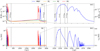 |
Fig. 3 Evolution of the accretion rate (panel a) and the position of the dead zone inner edge at the midplane (panel b) for the four different models analysed in this work. Panels a1 and b1 show a zoom-in to the time frame in which the TI-induced accretion event is occurring in the MREF model. The vertical dashed lines in panel a1 indicate the times corresponding to the ignition of the TI (tTI), the heating front reaching its largest extent and a cooling front starting to develop (tc), the retreat of the cooling front towards the star (tret) and the ignition of the first reflare (trefl). In panel a, the vertical dashed lines mark the points in time for which the surface profiles of the MREF model in panels b (tcut1 ) and d (tcut2) of Fig. 2 are shown. |
Properties of the TI-induced accretion events occurring in the models MREF and M3. M1 and M2 do not accumulate enough mass to trigger the TI.
 |
Fig. 4 Temperature maps (upper row) and corresponding surface density profiles (lower row) for four snapshots in time during an outburst event. In the upper row, the black contour lines correspond to T = TMRI, the yellow ones to T = TS, and the green ones to a radial optical depth of τ* = 2/3. tTI is chosen to be the point in time at which the TI is triggered. The second column shows the state of the disc at the time the MRI active region has reached its largest extent during the main burst (tc). The third column represents the stage of the ignition of the first reflare (trefl), the maximum extent of which is reached at the time depicted in column four. The state of the disc shortly after the instability has ended is shown in column five. |
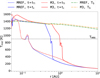 |
Fig. 5 Midplane temperature profiles of the MREF and M3 models at the time of the onset of the TI (tTI) and at the time at which the cooling front develops (tc). |
3.3 Surface density evolution and pressure maxima
The disc material in the vicinity of the ionisation front is redistributed according to the difference in angular momentum transport efficiency between the MRI active and inactive regions. Consequently, a sink in the surface density distribution develops behind the ionisation front while a corresponding spike travels ahead of the front. This behaviour is visible in the bottom panel of the second column in Fig. 4. As soon as the ionisation front has reached its largest radius and is reflected as a cooling front, the spike in surface density is left behind. Due to the decreasing magnitude of the consecutive reflares, every reflare places a density bump at the outer border of its respective MRI active region. The result after the TI phase has ended is a ‘saw-toothed’ surface density structure in the dead zone area ignited during the TI. This structure is shown in the bottom panel of column five in Fig. 4. Every spike in the surface density is associated with a corresponding maximum in the midplane gas pressure distribution.
Panel a of Fig. 6 is a space-time diagram of the model MREF where the surface density is shown in colour. The white contour lines indicate the location of pressure maxima in the disc mid-plane. The stable contour during the quiescent phase at a radius of 0.15 AU is the pressure maximum equivalent to the pebble-and migration trap identified by Flock et al. (2019).
A zoom-in to the time frame of the TI developing after 2520 yr is provided in panel b of Fig. 6. In addition to the pressure maxima, the dead zone inner edge movement at the midplane is depicted as a cyan contour line. The pressure bumps are placed at the radii where the dead zone inner edge reaches its largest extent. During the burst, the stable pebble trap present in the quiescent phase is disrupted and develops again after the TI has ended. The midplane pressure maxima placed in the dead zone by the TI can be fitted with an analytical function of the form (e.g. Taki et al. 2016; Lee et al. 2022; Lehmann & Lin 2022)
![Mathematical equation: ${P_{{\rm{mid,fit}}}} = {P_0}{\left( {{r \over {1\,{\rm{AU}}}}} \right)^a}\left[ {1 + b\exp \left( { - {{{{\left( {r - {r_{{\rm{Pb}}}}} \right)}^2}} \over {{{\left( {wH\left( {{r_{{\rm{Pb}}}}} \right)} \right)}^2}}}} \right)} \right],$](/articles/aa/full_html/2024/12/aa51175-24/aa51175-24-eq19.png) (18)
(18)
where  describes the underlying power-law structure of the midplane pressure profile in the vicinity of rPb which is the radial location of the pressure bump. H(rPb) is the disc scale height at rPb, calculated as
  , with pmid being the midplane density at the pressure bump. b and w are dimensionless parameters, representing the amplitude and breadth of the pressure bump, respectively. For instance, in the case of the pressure maximum at r = 0.6 AU, created by the first outward-travel of the ionisation front, the fitted parameters b and w equate to 1.9 and 2.0, respectively. The density and pressure maxima decay rapidly due to viscous diffusion and disappear after 113 yr, which corresponds to about 240 orbits. In contrast, b and w for the second pressure bump at r = 0.47 AU, resulting from the first reflare, yield 0.9 and 1.4, respectively, and the maximum decays after 150 yr or 460 orbits.
The space-time diagram for the model M3 is shown in panel b of Fig. 6. In this case, the dead zone is more massive at t = tTI and the ionisation front can travel further outwards. The TI starts to develop after 2350 yr and the first cycle deposits a pressure and density bump at a radius of 1.08 AU with the parameters b and w, resulting in 2.0 and 1.7, respectively. The viscous accretion process drags the pressure bump towards 0.9 AU, where it disperses after 390 yr, which equates to about 400 orbits.
Panel c of Fig. 6 depicts the space-time diagram for M2. Even after 5000 yr, the TI was not triggered and the pebble trap at 0.15 AU, slightly outside the location of the dead zone inner edge, persists undisturbed.
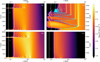 |
Fig. 6 Space-time diagrams of MREF (panel a), M3 (panel b) and M2 (panel c) with the colours corresponding to the surface density at the respective locations and times. While a TI cycle develops within a 3000 yr time frame in the MREF and M3, the M2 model does not show signs of TI even after about 5000 yr and the disc has reached a quasi-steady state. The white contours indicate the positions of pressure maxima. Panel a1 shows the space-time diagram of the TI phase of the MREF model. The cyan contour line corresponds to the location of the inner edge of the dead zone at the midplane. |
3.4 S-curve and reflares
Every simulation computed for this work shows the occurrence of multiple reflares during the evolution of a TI-triggered episodic accretion event. The development of this phenomenon has been studied in the context of S-curves in the Σ – Teff plane, which represent a visualisation of thermal stability (or instability) of the disc at a certain radius. In Fig. 7, we show such an S-curve for the model MREF at a radius of 0.2 AU. This location is situated in the dead zone, slightly outside the radius at which the TI is triggered. Instead of Teff, we show the midplane temperature, Tmid, since the midplane is where the TI elevates the temperature above TMRI first during the expansion of the ionisation front. The lower stable branch (‘low-state’ of the disc), which corresponds to the MRI being inactive at this location (i.e. α = αDZ), consists of data points extracted during the quiescent state (black dots) and during the burst phase when the heating front has not reached 0.2 AU yet. As soon as the MRI is activated, the disc quickly switches to the upper branch of the S-curve where α = αMRI (‘high-state’). The maximum temperature of the upper branch is capped by the dust sublimation temperature at which an equilibrium state between heating and cooling is manifested. The surface density spike just before reaching the upper branch corresponds to the mass pile-up ahead of the ionisation front. As the mass is efficiently drained onto the star, the model moves along the upper branch towards smaller surface densities and smaller temperatures. After the kink in the upper branch, which is where the temperature drops below TS, the midplane temperature decreases further towards TMRI = 900 K. While travelling along the upper branch, the tracks for the different cycles mostly overlap. As soon as the surface density decreases below a critical value,  , the model drops back down to the lower branch. In this context,
  is the minimum value of the surface density at which the MRI can be sustained. The S-curve shows that this critical value is the same for every cycle. After the last reflare (blue dots), the disc returns to the quiescent state and evolves along the lower branch.
Figure 8 depicts the surface density profiles of MREF and M3 at certain points in time during the burst phase. The times are also marked in panels a1 and b1 of Fig. 3 for the example of MREF. tc corresponds to the time at which the outward-moving ionisation front is reflected into an inward-moving cooling front. This occurs as soon as the minimum value in the surface density valley at the heating front reaches  , which is shown as a green profile. Below
  , the MRI can no longer be sustained and a decreases, which diminishes the efficiency of viscous heating and the material cools down. This leads to the development of a cooling front with the density valley retreating towards the star. Snapshots of the surface density of MREF and M3 during this time (t = tret) are shown as dotted lines in Fig. 8. The minimum value of the retreating surface density valley is equal to the local value of
  . The fit for
  shown in Fig. 8 has the form
![Mathematical equation: $\matrix{ {\Sigma _{{\rm{crit}}}^{\min } = 1678\left[ {{\rm{g}}{\rm{c}}{{\rm{m}}^{ - 2}}} \right]{{\left( {{{\log }_{10}}\left( {{r \over {1\,{\rm{AU}}}} + 1} \right)} \right)}^{0.856}}} \hfill \cr { - 9 \cdot {{10}^{ - 12}}\left[ {{\rm{g}}{\rm{c}}{{\rm{m}}^{ - 2}}} \right]{{\left( {{{\log }_{10}}\left( {{r \over {1\,{\rm{AU}}}} + 1} \right)} \right)}^{ - 8.582}},} \hfill \cr } $](/articles/aa/full_html/2024/12/aa51175-24/aa51175-24-eq28.png) (19)
(19)
where the power law component of this function outside of ~0.12 AU is proportional to r07. The drop of the  profile at r < 0.1 AU is related to the heating by irradiation: Close to the star, the importance of the irradiation heating relative to the heating by viscous dissipation increases, especially as the density in the inner disc decreases due to the accretion process. As a result, the surface density necessary to keep the disc MRI active becomes smaller.
In addition to the deviation of the  profile from a pure power-law close to the star, another effect of irradiation is the shift of the critical surface density for the ignition of a reflare,
  . This value is given by the position on the S-curve at which the disc leaves the lower branch. The corresponding point in time is denoted with trefl. In our models, all reflares are ignited at the same radius, so in order to visualise the different values of
  for subsequent reflares, the S-curve can be evaluated at this radius. We emphasise that the reflares do not constitute a strict ‘reflection’ of the cooling front into a heating front. Instead, the cooling front moves through towards the inner dust rim and the TI is triggered again (‘reignited’) in the cooled-down area, leading to another outburst cycle. On the other hand, the density wave travelling alongside the cooling front can be treated as being directly reflected.
Analogously to Fig. 7, panel a of Fig. 9 shows the S-curve of the model MREF, but at a radius of 0.091 AU, which is where the reflares are reignited. Since this area of the disc never becomes fully MRI inactive except for a very short time after the cooling front has passed through, the majority of the lower branch is missing in the depicted S-curve. Instead, the model switches back to the upper branch almost immediately after dropping down. The surface density value at which this occurs is not the same for every reflare; that is,  is smaller for later reflares. While a smaller density leads to less effective viscous heating, it also reduces the radial optical depth from the star towards the reignition radius. Consequently, the τ = 2/3 surface is located further outwards. In combination with a steeper irradiation angle onto the τ = 2/3 surface at the reignition radius, this leads to more rigorous heating by irradiation, compensating for the decrease in the effectiveness of viscous heating. To test the effect of irradiation on the reflare behaviour, an additional simulation was conducted in which the heating by irradiation was switched off. Again, multiple reflares occur with the reignition radius being closer to the star by a small margin. The S-curve of this model at the reignition radius is shown in panel b of Fig. 9. Without the effect of irradiation heating, the value of
  is the same for every reflare.
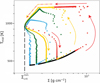 |
Fig. 7 S-curve of the MREF model at a radius of 0.2 AU. The black line corresponds to the evolutionary track during the quiescent phase, while the coloured dots are taken from snapshots during the outburst stage. The red data points were extracted during the first outburst and the yellow, green and blue dots make up the evolutionary tracks during the first, second and third reflare, respectively. The density of the dots along an evolutionary track indicates the velocity at which the disc evolves. The arrows are exemplary for the first two cycles and indicate the direction in which the model evolves. The surface density value at which the disc switches from the upper branch (where α = αMRI) to the lower branch (where α = αDZ) is the same for each cycle and is marked with |

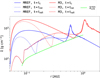 |
Fig. 8 Surface density profiles of the models MREF and M3 for three points in time each. tc, tret and trefl correspond to the points in time described in Fig. 3. The fit for the minimum values of the surface density valley travelling alongside the cooling front |

4 Discussion
The simulations conducted in this study combine heating by viscous dissipation and irradiation with the evaluation of the dust-to-gas mass ratio and tracking of temperature-dependent levels of turbulence at every position in the computational domain. Our results show that for disc masses that are large enough, the inner disc is prone to TI, which disrupts the vertical and radial temperature, density, and pressure structure. In this section, we analyse the implications of these disturbances and investigate the peculiarities of the TI phase in more detail. The analysis includes a discussion of the relevance of the pressure bumps emerging in our models, the variation in the dust content during the high-state of the disc, the potential impact of the TI evolution on the thermal history of solids in the disc, and the potential reasons behind the occurrence of reflares. We also compare our models to previous studies and point out limitations that our models are subject to.
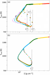 |
Fig. 9 S-curves during a TI-induced accretion event for the MREF model with (panel a) and without (panel b) the effect of irradiation heating, calculated at the respective radii at which the reflares are ignited. These radii are 0.091 AU and 0.087 AU for panel a and panel b, respectively. The data points with red, yellow, green, blue and pink colours were taken during the first, second, third, fourth and fifth reflare, respectively. With irradiation heating, the later reflares are ignited at smaller surface densities than the first three. The different critical surface density values are marked with |


4.1 Pressure bumps as possible sites of planetesimal formation
When the heating front travels through the inner disc towards larger radii, it sweeps over the area in which a large amount of mass has been accumulated during the quiescent phase. The strong increase in turbulent viscosity significantly enhances the transport of angular momentum in this high-density region. As a consequence, the heating front is accompanied by a density wave: The density behind the front is diminished while the material is compressed ahead of the front, creating a density bump (‘snowplough-effect’, Lin et al. 1985). When the heating front reaches its largest extent, this bump is left behind at that location while the cooling front retreats back towards the star. This maximum in density causes an analogous maximum in the gas pressure distribution, which, in turn, creates an area of super-Keplerian motion. The gas drag on dust particles then stops the inward flow of solid particles, creating a dust trap at the location of the pressure bump, similar to the dust trap created outside the orbit of a massive planet (e.g. Lambrechts & Johansen 2014). In the cases described in this work, the pressure bumps evolve on the viscous timescale in the dead zone with a stress-to-pressure ratio of αDZ = 10−3.
To estimate how much mass can potentially be trapped in the pressure bumps occurring in our models and how the density of dust may be altered at these locations as a consequence, we use the pebble flux predictor tool4 (Drazkowska et al. 2021) and calculate the mass accumulation in the strongest and most persistent pressure bump found in the model M3. The conditions in the disc around 1 AU, which is where the pressure bump is located, result in a pebble flux of 10−3M⊕ yr−1 and a Stokes number of St = 0.01. As an initial pebble-to-gas mass ratio in the midplane, we assume 0.01. The pressure maximum persists for about 390 yr, which is enough time to potentially trap 0.39 M⊕ of pebbles. The dust scale height, Hd, can be calculated according to (Flock & Mignone 2021)
 (20)
(20)
where H = cs/Ω is the gas pressure scale height and S c is the Schmidt number, which is set to unity. We assume that the region in which the dust accumulates is a torus with a major radius of 1 AU and a minor radius of Hd. Dividing the total accumulated mass after the pressure bump lifetime by the volume of the torus results in a mean dust density of ρd,mean = 8.7 ⋅ 10−11 g cm−3. Next, we imposed a Gaussian distribution on the dust accumulating with a standard deviation of Hd/3, so that the maximum dust density is located in the centre of the torus (i.e. at the mid-plane). This maximum value can be calculated by equating the volume under the Gaussian function to the volume of a cylinder with a base of radius Hd and a height of ρd,mean,
 (21)
(21)
For the main pressure bump produced by the TI in the model M3, the maximum pebble density at the bump location yields 4 ⋅ 10−10 g cm−3. The gas density in the area of the torus has values around 8.8 ⋅ 10−10 g cm−3, which leads to a maximum solid-to-gas mass ratio of 0.45 at the midplane. Vertically integrating the Gaussian function for the pebble distribution at the pressure bump location results in a solid surface density of 100 g cm−2. Considering that the gas surface density at that location lies at 1900 g cm−2, this leads to a vertically integrated solid-to-gas mass ratio (also referred to as the metallicity Z ) of 0.052. Following the empirical relation found by Yang et al. (2017) for St < 0 1
 (22)
(22)
the critical solid-to-gas mass ratio above which significant spontaneous concentration of solids can occur results in a value of 0.017 for a Stokes number of 0.01. Since Z > Zcrit in the case of the analysed pressure bump occurring in our models, streaming instability may become efficient and can quickly raise the solid-to-gas mass ratio beyond unity (e.g. Simon et al. 2016; Flock & Mignone 2021).
The above calculation has been conducted under the assumption that the pressure bump stays at the same location and is capable of trapping all inward-drifting solids throughout its entire lifetime. Therefore, the result should be seen as an upper limit. With the parameters of our model and the method described above, the pressure bumps created by the heating front during the TI may be capable of accumulating enough solids to induce streaming instability. Therefore, the TI mechanism analysed in our models can provide a possibility to form planetesimals over an extended radial range in the inner disc. However, it is worth pointing out that the turbulent α parameter of 10−3 in the dead zone of our models may cause significant stirring around the midplane and inhibit the development of the streaming instability (e.g. Li et al. 2022; Lesur et al. 2023). On the other hand, the considerations above take the rather high value of α into account during the calculation of Hd. Furthermore, the level of turbulence usually decreases when approaching the midplane (e.g. Flock et al. 2017b), so α = 10−3 might be an overestimation for the conditions near the midplane. Additionally, a higher Stokes number of 0.1 (i.e. assuming larger solid bodies) can significantly increase the amount of accumulated matter such that the solid-to-gas mass ratio at the end of the pressure bump’s lifetime takes on values which favour the development of the streaming instability even more. A full evaluation of the conditions concerning streaming instability in the pressure bumps occurring in our models requires dedicated simulations, including coupled gas and dust dynamics during the evolution of the pressure bump, as well as self-consistent treatment of local levels of turbulence.
Another possibility to form planetesimals in regions of enhanced dust concentration is the direct gravitational collapse of the dust cloud (e.g. Johansen et al. 2006). However, to fulfil the conditions for this formation process, the gas disc has to be marginally gravitationally unstable already (e.g. Baehr 2023). In our models, the Toomre parameter in the disc regions around the density maxima placed by the TI evolution is of the order of 102 even for the most massive disc model (M3). Following Gerbig et al. (2020), a similar stability criterion can be formulated for the gravitational stability of a dust clump, which depends on the Toomre parameter, the metallicity, Z, the efficiency of dust diffusion, and the Stokes number. The conditions for GI are fulfilled when the stability parameter, Qp, is smaller than unity. Applying this criterion to the strongest density bump in the model M3 results in Qp > 102. Therefore, we can assume that the dust concentrations formed in our models are gravitationally stable.
4.2 An equilibrium dust density in the high-state region
The description of the dust-to-gas mass ratio, fD2G, given in Eq. (15) is adequate for applications to irradiated inner discs with a resolved inner dust rim. However, a subtle difficulty arises when significant viscous heating during the TI phase is also considered. In the area of the disc in which τ* > 3, a jump in fD2G is manifested at TS, which does not take effect in a purely irradiated disc because temperatures in the vicinity of TS are not expected beyond τ* = 3. During a TI-induced accretion event, viscous heating is indeed capable of raising the temperature beyond TS in the optically thick regions around the midplane. In these cases, when the temperature increases above TS, fD2G switches from f0 to a value dominated by f∆τ, which was only constructed for resolving the inner dust rim and should not have an influence on other disc regions. Since f∆τ is small, the cooling efficiency abruptly increases, which leads to a stabilisation of the temperature at TS. In order to evaluate a more realistic dust density during the high-state of the disc, we updated the prescription for the dust-to-gas mass ratio,
![Mathematical equation: $\matrix{ {{f_{{\rm{D}}2{\rm{G}}}} = \left\{ {{f_{\Delta \tau }}{1 \over 8}\left[ {1 - \tanh \left( {{{\left( {{{T - {T_{\rm{S}}}} \over {150{\rm{K}}}}} \right)}^3}} \right)} \right]\left[ {1 - \tanh \left( {2/3 - {\tau _*}} \right)} \right]} \right\}} \hfill \cr { \cdot \left\{ {1 + \tanh \left( {{{3.0 - {\tau _*}} \over {0.4}}} \right)} \right\}} \hfill \cr { + \left\{ {{f_0}{1 \over 4}\left[ {1 - \tanh \left( {{{T - {T_{\rm{S}}}} \over {20{\rm{K}}}}} \right)} \right]} \right\}\left\{ {1 - \tanh \left( {{{3.0 - {\tau _*}} \over {0.4}}} \right)} \right\}.} \hfill \cr } $](/articles/aa/full_html/2024/12/aa51175-24/aa51175-24-eq42.png) (23)
(23)
This new function smoothly combines the evaluation of fD2G in the region around the dust sublimation front (τ* < 3) and the optically thick outer disc (τ* > 3). There is now a smooth transition at TS beyond τ* = 3, where fD2G is independent of f∆τ and only depends on f0 and the temperature. This allows fD2G to smoothly and freely adopt a value that results in an equilibrium between heating and cooling in the high-state region. To analyse the effects of this new description on the adaptation of the dust density, we created two additional models MREF* and M3*, which are set up in the same manner as MREF and M3 but include the function given in Eq. (23) for evaluating fD2G. In Appendix B, we illustrate the behaviour of this new description and show that its influence on the TI onset and evolution is minimal.
Figure 10 depicts radial profiles of various properties of MREF* and M3* during the evolution of an accretion event. The points in time that these profiles represent have been chosen such that the stage of the TI evolution is different: The profile of MREF* has been taken at the time the first reflare has reached its largest extent, while the M3* profile shows the stage of the disc during the first expansion of the heating front. Panel a shows the gas and dust surface densities. The radii at which the solid lines (1000 ⋅ Σd, where Σd is the dust surface density) join the dashed lines (gas surface density, Σg) is the outer boundary of the region in which the temperature exceeds TS. The midplane and dust sublimation temperatures for these two models are shown in panel b. The blue line indicates that Tmid has reached an equilibrium value in the highly viscous region when the heating front has reached its largest extent, and the inner disc has had enough time to adapt to the conditions on the upper branch of the S-curve. In the M3* model snapshot, the accretion rate at small radii has not yet fully adapted to the high turbulence and the equilibrium temperature has only started to manifest itself.
We now aim to find a relation that connects the dust surface density in the fully ignited regions to other typical physical quantities. Since the dust surface densities seen in panel a of Fig. 10 are a result of the equilibrium between heating and cooling in the respective regions, they have to depend on parameters which govern heating and cooling mechanisms in our disc model. In the high-state regions, heating is dominated by viscous dissipation, which mainly depends on the density, temperature and velocities (with the largest contribution coming from the angular velocity). The efficiency of radiative cooling is given by the optical depth, which again depends on the density and temperature around the ignited regions. Therefore, to first order, the dust surface density in the fully ignited, high-state equilibrium regions should be expressible in terms of the gas surface density Σg and the pressure scale height H. The profiles of the pressure scale height are depicted in panel c of Fig. 10 for the two representative cases and show that the disc adapts itself so that the scale height at a given radius in the ignited disc regions in which T > TS (i.e. in which an equilibrium temperature is reached) is the same for each model and every stage of the TI phase. A simple power-law fit to this profile of the scale height in these regions of the disc results in
 (24)
(24)
Based on this finding, the dependence of the dust surface density on H can be transformed into a dependence on r. Fitting a power-law function to the dust surface densities in the high-state equilibrium regions results in the following relation,
 (25)
(25)
The parameters given in this equation have been evaluated based on a large number of snapshots at different stages during the TI evolution in the MREF* and M3* models. The dotted green lines in panel a of Fig. 10 show the fit for one representative point in time for each model.
We emphasise that the relations given in Eqs. (24) and (25) are a result of the parameters chosen for the model setup described in this work. A different description of the dust and gas opacities as well as a different choice of the viscosity parameters, αMRI and αDZ can have a significant influence on the dependencies and numerical parameters in these expressions.
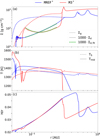 |
Fig. 10 Radial proflies of the surface density (panel a), the temperature (panel b) and the pressure scale height (panel c) within 1 AU for one representative point in time each during the TI development in the MREF* and M3* models. In panel a, dashed lines represent the gas surface density, Σg, solid lines show the dust surface density, Σd, and the dotted lines depict the respective fits to the dust surface density, Σd,fit, in the high-state region, evaluated with Eq. (25). Σd and Ed,fit are multiplied by 1000 to compensate for the baseline dust-to-gas mass ratio ƒ0 and make the values comparable to Σg. The solid lines in panel b correspond to the midplane temperature, while the dashed lines represent the dust sublimation temperature. |
4.3 Comparison to previous works
Two-dimensional simulations of the protoplanetary discs in the r–θ plane during the TI stage have been carried out by Wunsch et al. (2005), who also utilise a radiation hydrodynamic model of a layered disc with a flux-limited diffusion approximation of the radiation transport and an MRI activation temperature of 1000 K. The main differences between their set-up and our model are the opacity description, the absence of irradiation heating in their models and the size of their computational domain. Instead of separating the total density in the disc into a dust and gas component via a prescription for the dust-to-gas mass ratio, they used the opacity relation given by Bell & Lin (1994) for a gas-dust mixture. The results of their Model 5 most closely resemble the evolution of our models since they implemented the same αMRI/αDZ ratio, which controls the rate of mass accumulation at the dead zone inner edge. The Tl-induced accretion event occurring in their Model 5 is considerably less massive, entailing an amplification of the accretion rate by a factor of 6, compared to our cases with amplification factors of over 200. Interestingly, Wunsch et al. (2005) do not observe reflares in the same manner as they appear in our simulations. However, they derive a relation describing the critical surface density below which an MRI active disc cannot be sustained, which corresponds to  in the nomenclature of our work. They find that this critical value scales with ~r0.75, which is close to the scaling we derive for
  in the region dominated by viscous heating (~r0.7).
A similar relation has been derived by Nayakshin et al. (2024) for protoplanetary discs. Contrary to our model, the TI occurring in their simulations is based on a strong increase in the gas opacity at temperatures larger than 2000 K (as included in the opacity description given by Bell & Lin 1994), which is associated with the ionisation of hydrogen. In order to achieve such temperatures in the inner disc, they induced a continuous mass flux into the disc through the outer boundary at a rate of > 10−7 M⊙>yr−1, which is not necessary for our models. They calculated S-curves for the vertical thermal stability of the disc structure at different radii and deduced a scaling for  and
and  with respect to the radius of ~r0.96. Considering that the TI mechanism has a different origin and the conditions in the disc, both in the low- and high-state, are different compared to our models, the discrepancy between their scaling relation and the one derived from our models is not surprising. However, reflares are occurring in some of their models. We explore this phenomenon further in Sect. 4.4.
The TI observed in the models of Nayakshin et al. (2024) is analogous to the classic disc instability model (DIM) for cataclysmic variables such as dwarf novae or X-ray transients (e.g. review by Hameury 2020). In the context of protoplanetary discs, this kind of TI has been explored by Pavlyuchenkov et al. (2023), who conclude that there are indeed multiple solutions for the disc’s thermal structure under the conditions in which the gas opacity is strongly dependent on temperature. This results in the typical S-shape of the thermal equilibrium curves in the Σ–T plane. If such a disc is evolved in time, including a viscous α prescription, outbursts comparable to FU Ori events can occur. However, such conditions require surface densities and midplane temperatures that are not reached in our simulations. Nevertheless, the TI induced by the activation of the MRI with the descriptions used in our models results in a comparable limit cycle manifested as S-curves in the Σ – Tmid plane (see Fig. 7). In our models, the unstable branch of the S-curve, connecting the stable low-state and high-state equilibrium branches, is a consequence of the viscous α parameter (instead of the gas opacity) becoming dependent on temperature in the vicinity of TMRI (according to Eq. (13)). This instability is also indicated in the models of Jankovic et al. (2021). They report that in the regions of the inner disc where the MRI becomes quenched (corresponding to the inner edge of the dead zone), they find multiple solutions for an equilibrium of the vertical thermal structure. Similarly, Mohanty et al. (2018) find that their steady-state solutions might be viscously unstable due to a change in the vertically integrated stress-to-pressure ratio as a function of the mass flux.
Both versions of the TI were combined in a two-dimensional axisymmetric model by Zhu et al. (2009b). Since they aimed to explain and recreate observational signatures of FU Ori-type outbursts, the accretion rates, densities and temperatures are significantly higher compared to our models. Additionally, they did not consider irradiation by the central star or a fully MRI active disc at small radii. Instead, accretion in the innermost disc during quiescence is only driven by a mass flux in the ionised surface layers and the MRI is eventually activated beyond 1 AU by the accumulation of mass through an inward transport by GI, governed by a viscous α prescription. After the MRI becomes active and the accretion event is initiated, the temperatures increase so that the TI induced by hydrogen ionisation occurs as well. Although the objects considered by Zhu et al. (2009b) are younger and more massive than the ones investigated in our simulations, and the burst is triggered by a different mechanism, the shape of the MRI active zone in the high-state during the outburst event generally agrees with our findings.
Another radiation hydrodynamic model of the inner regions of a protoplanetary disc in two-dimensional axisymmetric geometry has been investigated by Flock et al. (2016). The set-up of their simulations is very similar to the one presented in this work. However, they considered Herbig Ae stars as the central objects, which exhibit luminosities of 56 L⊙. Consequently, the inner dust rim and the inner edge of the dead zone are shifted to much larger radii compared to our models, which considerd a star with a luminosity of ~2 L⊙. While in our simulations, the stable pressure maximum at the dead zone inner edge during the quiescent state of the disc is situated at 0.15 AU, its location is shifted to 0.9 AU in the dynamic simulations of Flock et al. (2016). At such distances, viscous heating is less effective and the required density to initiate the TI is much larger than the values they achieve. As a consequence, the discs do not become thermally unstable and remain in the low-state.
The development of pressure bumps as a result of accretion events induced by MRI activation in the dead zone has also been documented by Chambers (2024). They describe the evolution of fast- and slow-moving waves, which correspond to the movement of the heating or cooling front and the viscous evolution of the density maxima analysed in this work, respectively. The lifetime of the pressure bumps corresponding to the slow-moving waves is of the order of a few thousand years, which is longer than the existence of the pressure bumps occurring in our simulations after the TI. The reasons for this discrepancy are a larger value of αDZ implemented in our simulations, the smaller radius at which the bumps are situated initially and the absence of a pressure gradient force on the motion of the gas in the model of Chambers (2024). They speculate as well that the pressure maxima in their models may be capable of initiating streaming instability. We continue to build on this idea in Sect. 4.1.
Brož et al. (2021) investigated the formation of the architecture of the terrestrial planets in the solar system and found that models of convergent migration towards 1 AU provide a promising prospect. Interestingly, they indicate that the surface density structure required for such a migration mechanism should have a peak at 1 AU. Such a distribution looks remarkably similar to the disc structure of our models just after the TI phase (especially regarding the M3 model; see panel d of Fig. 2). However, the surface density profile changes throughout the quiescent phase as the inner disc is replenished with material from larger radii and the peak is smoothed out (in the case of M3) or disappears (in the case of MREF; see panel c of Fig. 2). Only after a TI cycle, a clear peak around 1 AU is reinstated. In order to combine the idea of convergent migration with a disc prone to outbursting events, dedicated simulations are required that include the migration of planetary bodies during and after the stage of the disc evolution in which outbursts occur.
4.4 Possible origins of reflares
Reflares are a well-known phenomenon in the context of disc instability models for cataclysmic variables (Lasota 2001; Coleman et al. 2016; Hameury 2020). They are typically considered as a weakness of the DIM since observations of rebright-enings after a main burst are rare for dwarf novae and X-ray transients. Reflares have also been reported in simulations of pro-toplanetary discs under certain conditions during the evolution of FU Ori-type outbursts (Nayakshin et al. 2024). All models analysed in our work show the occurrence of reflares.
They are typically characterised as a ‘reflection’ of the cooling front into a heating front. In our models, however, the disc region between the inner dust rim and the location at which the heating front starts moving outwards again also begins to cool down. The temperature then strongly increases again at a radius of 0.091 AU for the MREF and M3 models, launching a new heating front in all directions, which can be described as a ‘reig-nition’ of the TI rather than a reflection of the cooling front. As is argued by Coleman et al. (2016), the reason for this phenomenon could lie in the specific shape of the S-curve and the value of the viscous α parameter in the high-state of the disc. If the difference between  and
and  is too small, the surface density behind the inward-moving cooling front can eventually become larger than
  and the TI starts anew. On the other hand, a very high value of αMRI enables more efficient draining of the ignited disc material on the star, which reduces the post-cooling-front density and could inhibit the occurrence of reflares. However, αMRI = 0.1, as used in our models, is already at the upper limit for MRI active zones (e.g. Flock et al. 2017b). A smaller value for αDZ could, in principle, shift
  to larger values, therefore increasing the difference between the two critical surface density values. This would also lead to a more massive outburst due to the large density necessary for triggering the TI and the heating front being able to travel to larger radii. Another factor for determining the shape of the S-curve and the critical surface density values is the function controlling the switch between αMRI and αDZ (Eq. (13)): A broader temperature range within which α is dependent on the temperature can contribute to the difference between
  and
and  and can possibly have an influence on the reflare behaviour.
In addition to these factors, Nayakshin et al. (2024) find that reflares tend to disappear for smaller values of the critical temperature around which α changes between the low-state- and high-state values. A change in TMRI does not influence the values of the critical surface densities significantly, but it has an impact on the shape and position of the unstable middle branch of the S-curve, which they deem vital for the emergence of reflares. In our models, we have chosen a relatively low value for TMRI (Desch & Turner 2015). However, since the mechanism for triggering the TI in the set-up of Nayakshin et al. (2024) is due to a strong dependence of the gas opacity on the temperature and the values for the critical temperature are of the order of 104K in contrast to 900 K used in our simulations, the comparison between their models and ours in the context of the occurrence of reflares might not be accurate.
Since the onset of the TI not only depends on the efficiency of viscous heating but also on the effectiveness of heat-trapping in the vicinity of the inner dead zone edge, it is worth considering the evolution of the opacity of the material near the midplane in the time frame within which a reflare is ignited. Interestingly, a reflare is ignited at almost the same time at which the temperature drops below Ts at every location beyond the dust sublimation front. This suggests that a more effective heat-trapping near the midplane caused by a sudden increase in optical depth by condensation of dust may be responsible for the reignition of the TI. However, we conducted several tests in which the optical depth in the vicinity of the location of the reignition was kept at a low level artificially and did not observe significant changes in the reflaring behaviour.
Irradiation by the central star only marginally affects the emergence of reflares. As is shown in Sect. 3.4 and Fig. 9, the location of the reignition is closer to the star and the two critical surface density values do not change for different reflare cycles if the heating by stellar irradiation is not considered.
The location of the computational domain’s inner boundary is another relevant factor for investigating the occurrence of reflares. In our models, the innermost part of the disc is always on the upper branch of the S-curve, making it difficult for the cooling front to reach the inner boundary. The hot material in the inner MRI active disc creates a density and corresponding pressure maximum while being accreted onto the star during the outburst cycle (see Figs. 8 and panel al of 6). Even though the value of αMRI is chosen to be large, the accretion process is not effective enough to diminish this density and pressure bump quickly enough. As the cooling front travels back towards the star, the pressure bump may still be too strong for the incoming density and pressure waves to cross over. Therefore, the density wave may partly be reflected and could deposit additional material behind the cooling front, enough to trigger the MRI and launch a new heating front. If the inner boundary was chosen to be located at larger radii, more of the material making up the pressure bump may cross over the boundary and get accreted onto the star, making the reflection of the incoming density wave less likely.
In summary, reflares emerge due to the surface density behind the retreating cooling front crossing a critical value  , which is set by the interplay between viscous heating near the disc midplane and the inefficiency of radiative cooling and consequent heat-trapping. Therefore, the questions of why the post-cooling-front surface density is high enough and why the value of
  is low enough need to be considered when evaluating the origins of the reflaring behaviour. To answer these questions, investigations of the parameter space of possible αDZ and αMRI values, as well as variations and improvements in the descriptions for the opacities and dust-to-gas mass ratio, may be crucial. These considerations go beyond the scope of this paper and will be part of future work.
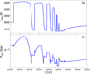 |
Fig. 11 Evolution of the midplane temperature (panel a) and midplane total gas pressure (panel b) at the location of the pebble trap (at 0.15 AU) during a TI-induced accretion event. |
4.5 Thermal processing of solids
The thermal history of a protoplanetary disc plays an important role in the nucleosynthetic composition of solid bodies in planetary systems (e.g. Scott 2007; Trinquier et al. 2009). Hereby, chondrules and calcium-aluminium-rich inclusions (CAIs) found in meteorites are of special interest, since their occurrence and abundance give clues about the thermal conditions under which they are formed in the disc (e.g. review by Scott 2007). The intricate composition of chondrules suggests that they have been subject to multiple rapid heating and cooling events during their formation, whereas condensation and subsequent coagulation of solids within ~2 AU from the star seem to be necessary to explain the CAI abundance and the depletion of moderately volatile elements in chondritic meteorites (Cassen et al. 2001). Connelly et al. (2012) argue that accretion processes might be capable of providing favourable conditions for chondrule formation in the inner disc. However, certain chondrule species only form late in the disc evolution (with disc ages of up to 3 Myr) when accretion rates are not thought to be large enough anymore to create the necessary high temperatures in the dusty disc regions. Dynamic crystallisation experiments indicate that temperatures just below the chondrule melting temperature (~1600 K) are required to create specific textures found in chondrules (e.g. Jones et al. 2018). Our models show that episodic accretion processes can repeatedly elevate temperatures towards this regime. Figure 11 shows the midplane temperature and gas pressure modulation during the accretion event at 0.15 AU, which is where the pebble trap is situated during the quiescent phase. Following Flock et al. (2019), we can assume that solid bodies accumulate at this location and may undergo the depicted temperature variations.
Panel a indicates that the midplane temperature can change rapidly by several hundred Kelvin during the evolution of the TI. For instance, after the first burst, the temperature drops from ~ 1400 K to below 600 K, after which it increases again during the first reflare towards 1400 K. The amplitude of the temperature fluctuations becomes smaller in later reflares. However, the required heating and cooling rates for chondrule formation are thought to be in the range of several 100 K h−1 (e.g. Jones et al. 2018), which is much larger than the ones resulting from our models. Here, the temperature increases by about 800 K over the course of one month while the cooling rates are even smaller. Furthermore, the temperatures in our models remain at levels close to the sublimation temperature for several years before cooling down, which is also in contrast to the required thermal processing of chondrules (e.g. Libourel & Portail 2018). Therefore, our TI models may be unfit to provide the appropriate conditions for chondrule formation.
It is worth noting, however, that the explanation of chondrule structures and composition is more complex. Libourel & Portail (2018) argue that the interaction of the solids with the surrounding gas component of the disc is essential and can allow for more moderate cooling rates. Furthermore, due to the highly dynamic process of the accretion event, it is unclear how the solid particles trapped near the inner dead zone edge are redistributed during and after the TI evolution. While a significant amount might be accreted onto the star, a part of the solid content may be transported to larger radii or higher disc layers by the expanding heating fronts and accompanying density waves. Therefore, the thermal history of individual particles cannot be inferred directly from the variations shown in Fig. 11. Explicit inclusion of dust particles with varying Stokes numbers in our models could provide essential insights into the thermal and dynamic evolution of solids in the disc.
Additionally, panel b of Fig. 11 shows the variation in the midplane total gas pressure. For instance, Tsuchiyama et al. (1999) describe different evaporation regimes for forsterite in discs, depending on the total gas pressure and the temperature. Therefore, the self-consistent calculation of temperature and pressure in disc regions undergoing strong dynamic and thermal variations could help in the analysis of the mechanisms and consequences of the evaporation of solids.
4.6 Model limitations
Although our models incorporate multiple important aspects concerning the evolution of the inner rim during and between phases of TI, specific limitations must be taken into account. Our initial models represent hydrostatic structures of inner pro-toplanetary discs based on the set-up of Flock et al. (2019). They do not include radial and vertical velocity fields and are already thermally unstable due to the effect of viscous heating. As a consequence, the disc immediately enters the TI phase after initiating the time-integration of the hydrodynamic equations. Although the evolution of the initial TI cycles closely resembles the ones occurring during the simulations, it is unclear to what extent they are influenced by our choice of the initial conditions. A steady-state initial model including velocity fields and with the disc located on the lower stable branch of the S-curve shortly before reaching  at the dead zone inner edge would certainly improve the quality of the beginning stages of the simulations.
In accordance with Flock et al. (2019), the opacity description of our models consists of averaged values for both the gas and dust opacities in order to properly resolve the inner dust rim. Using fitting functions for the opacities such as the ones given by Bell & Lin (1994) or Zhu et al. (2009a), or interpolating between pressure- and temperature-dependent values from tables (as provided by e.g. Malygin et al. 2014) could have an influence on the magnitudes of the accretion events and the timescales of the quiescent and TI phases.
In our models, the fraction of dust in the disc is considered to determine the optical thickness of the disc material. However, we neglect the drift, settling, and growth of different dust species of different sizes. Studies have shown that TI-induced accretion events may have a significant impact on these processes (e.g. Vorobyov et al. 2022). Additionally, considering dust evolution and distribution may help in understanding the importance of the pressure bumps placed throughout the inner disc during the TI cycles (e.g. Taki et al. 2016; Lehmann & Lin 2022). In a similar manner, the inclusion of the chemical evolution during and after outbursts can give valuable insights into the chemical composition of discs influenced by strong changes in the thermal structure (e.g. Rab et al. 2017).
The inner boundary of our computational domain is located at a fixed radius of 0.05 AU. However, Hartmann et al. (2016) argue that the description of disc accretion becomes inaccurate in the vicinity of the magnetic truncation radius, which is where the accretion becomes dominated by the stellar magnetic field. When equating the magnetic pressure from the stellar magnetic field to the ram pressure of the accreting material, the location of the truncation radius can be evaluated using the description given in Hartmann et al. (2016). Implementing a typical stellar magnetic field strength of 1 kG (e.g. Johns-Krull 2007) and the stellar parameters of this work given in Table 1 yields radii for disc truncation between 0.02 AU and 0.1 AU depending on the accretion rate during our simulations. Steiner et al. (2021) utilised this description for their inner boundary and found that its variability in combination with torques exerted on the disc by the stellar magnetic field (Romanova & Owocki 2015; Romanova et al. 2018) can change the outbursting behaviour.
Our models do not consider the effect of accretion shock luminosity. Assuming that about 50% of the gravitational energy of the accreted material is dissipated, the accretion luminosity in our models would increase from about 1% of the stellar luminosity during the quiescent state to a factor of a few larger than the stellar luminosity at the peak of the outburst. Although the heating in the optically thick regions is dominated by viscous dissipation during the TI evolution, this amplification of the irradiation could possibly facilitate the advancement of the heating fronts and have an influence on the dust evolution (Vorobyov et al. 2022) and thermal processing of solids throughout the disc (Colmenares et al. 2024).
Various magnetohydrodynamic effects can have a significant influence on the inner disc structure and evolution. Magnetocen-trifugal winds can be a major driver of accretion by removing angular momentum from the disc close to the star (Bai & Stone 2013; Lesur et al. 2023). During episodic accretion events, these magnetically driven outflows can be strongly amplified (Königl et al. 2011). Additionally, the removal of mass by winds could possibly help stabilise the disc against TI by reducing the surface density. Considerations of non-ideal magnetohydrodynamic effects in the context of the structure and evolution of the inner disc rim (Faure et al. 2014; Flock et al. 2017a) and the effectiveness of angular momentum transport via MRI (Bai & Stone 2013; Simon et al. 2018; Rea et al. 2024) could certainly help to improve our results as well. Moreover, Flock et al. (2013) have shown that a vertical profile of α, dependent on the volumetric density, replicates results from full radiation magnetohy-drodynamic simulations more accurately. Implementing such a vertical dependence could have an influence on the dynamics of the TI.
Furthermore, in our description of the stress-to-pressure ratio, an instantaneous response of α to a change in temperature is assumed. However, previous studies have indicated that the magnetic fields giving rise to the MRI only gradually build up and decay, leading to a significant delay between changes in the disc properties and the corresponding effect on the turbulent viscosity (e.g. Hirose et al. 2009; Flock et al. 2017a; Ross et al. 2017; Held & Latter 2022). In order to account for this effect, the description of a needs to be modified with a time-dependent factor. While such a modification has already been implemented in the models of Zhu et al. (2010) and Cleaver et al. (2023) in a simplified manner, the consideration of this effect in our simulations needs to be handled more carefully. The reasons for this claim are twofold: On the one hand, the TI evolution is mainly characterised by the outward expansion of the MRI active region. However, since the growth and decay rate of the MRI is a function of the orbital timescale, the outward-propagation of the heating front may be heavily impeded by this effect. This can have significant consequences for the characteristics of the accretion event and the formation and location of pressure maxima. On the other hand, our models include a highly turbulent inner gas disc. As a consequence, a transition between MRI active and inactive regions is present throughout the entire simulation. During the quiescent phase, this transition region may show a more dynamic behaviour than indicated by the models of this work because small perturbations in the disc structure cannot be smoothed out quickly by an a instantly reacting to changes. Instead, they may even be amplified or lead to continuous oscillations of the density and temperature structure. Consequently, the dead zone inner edge may hardly ever be a stable structure of the kind indicated by our models during the quiescent phases. Another possible result of these oscillations may be the variability of the accretion rate on timescales of the order of years and amplitudes of factors of a few. These interesting prospects can be investigated using a viscosity description that considers the gradual saturation of the MRI in the context of our models and will be investigated in detail in a forthcoming paper.
5 Conclusion
In this work, we have utilised axisymmetric 2D radiation hydro-dynamic simulations to investigate the vertical and radial structure and time-dependent evolution of the inner protoplanetary disc around a Class II T Tauri star. The models include an inner fully MRI active disc, a description for dust sublimation to resolve the inner dust rim, a transition towards a dead zone via a viscous a prescription, heating by stellar irradiation and viscous dissipation, and calculation radiation transport in the vertical and radial directions. Starting from a hydrostatic initial state, we tracked the evolution of TI triggered by MRI activation in the dead zone and analysed its effects on the disc properties. The main results of our study can be summarised as follows:
The inner disc is prone to TI as long as accretion heating and heat-trapping near the midplane can elevate the temperature to values at which a becomes dependent on the temperature, which leads to runaway heating and consequent activation of the MRI. Initial accretion rates of ≥3.6 ⋅ 10−9 M⊙ yr−1 can be sufficient to accumulate enough material at the dead zone’s inner edge to trigger TI;
The evolution of the TI creates an oblate-torus-shaped MRI active region in the inner disc that can extend up to 1 AU in the radial direction and 0.05 AU in the vertical direction symmetrically around the midplane. Within this region, temperatures become high enough for dust to begin to sublimate;
The instability disrupts the otherwise stable planetesimal and migration trap at the dead zone’s inner edge. The corresponding pressure maximum is reinstated only after the TI phase has ended;
Reflares are a robust outcome of our simulations. They occur due to the elevation of the surface density above a critical value behind the retreating cooling front as it approaches the inner dust sublimation region;
The instability cycle and reflares can be tracked on S-curves of thermal stability from which critical surface density values for the activation and quenching of the TI can be extracted;
The burst and the consequent reflares place pressure maxima at the respective locations where the outward-travelling heating front stalls. These bumps may be capable of trapping solid particles and can remain in the disc long enough to initialise streaming instability;
On the upper stable branch of the S-curve, the dust density adapts itself so that viscous heating and radiative cooling are in equilibrium. In the radial sections of the inner disc, where this is the case during the evolution of the TI, we find a simple relation between the gas and dust-surface densities.
Resolving the two-dimensional structure of the inner disc while carefully considering the vertical and radial transport of radiation vitally contributes to our understanding of the thermal and dynamic evolution of planet-forming regions undergoing TI. Despite certain numerical and physical limitations, our models provide a robust foundation for potential future investigations, which include improved viscosity descriptions, the consideration of dust evolution, the implementation of magnetohydrodynamic effects, and the creation of synthetic observations. The elaboration of these prospects will further illuminate the effects of TI on the formation and evolution of planets in protoplanetary discs.
Acknowledgements
We would like to thank Zhaohuan Zhu and Doug Johnstone for fruitful discussions about this work’s ideas. We thank the anonymous referee for their constructive and thoughtful comments. This research was supported by Deutsche Forschungsgemeinschaft (DFG) under Grant No. 517644750.
Appendix A Gas opacity
For our hydrodynamic simulations, we reevaluated the Rosseland mean gas opacity to account for more accurate values of gas density and temperature in the regions of the disc where gas dominates the opacity. In Fig. A.1 we show the area in the T - ρgas plane within which the corresponding opacity values are considered. Temperatures below ~ 800 K are irrelevant for these considerations because, in this range, dust will always dominate the opacity. The average value in the outlined region in Fig. A.1 amounts to κR = 10−3 cm2 g−1.
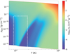 |
Fig. A.1 Visualisation of the Rosseland mean gas opacity coefficients given by Malygin et al. (2014). The dashed white rectangle indicates the density- and temperature regions for the gas from which the average value implemented in our simulations has been extracted. |
Appendix B Updated computation of ƒD2G
In this section we compare the new function for evaluating the dust-to-gas mass ratio, introduced in Sect. 4.2 and implemented in the model MREF*, to the original one given by Eq. 15. Figure B.1 shows a schematic illustration of both functions, evaluated based on a constant density profile and representative temperature- and optical depth profiles. Before reaching the radius where τ* = 3, the two functions do not differ significantly. Instead of a sharp jump to ƒ0 = 10−3 at τ* = 3 (which is largely exaggerated in Fig. B.1) in the original version, the new function produces a smooth transition. The largest difference reveals itself when the temperature crosses TS beyond τ* = 3. While ƒD2G instantaneously jumps to a value dominated by f∆τ and locks the temperature at TS in MREF, the new function lets ƒD2G smoothly adapt as TS is crossed.
Figures B.2 and B.3 show comparisons between MREF and MREF*, conducted with the full simulation set-up. While the quiescent stage is not influenced by the new function, the accretion event in MREF* is marginally more massive and the MRI- and dust sublimation transitions are manifested in a smoother manner. Otherwise, the structure and evolution of the burst are not affected.
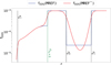 |
Fig. B.1 Schematic visualisation of the functions describing the dust-to-gas mass ratio in the MREF and MREF* models. For illustrative purposes, the density was held constant, representative profiles for the temperature and radial optical depth have been chosen and the models are shown as functions of a dimensionless radius. The vertical dashed black lines mark locations where the temperature crosses the dust sublimation temperature. |


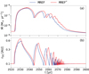 |
Fig. B.2 Evolution of the accretion rate (panel a) and the position of the dead zone inner edge at the midplane (panel b) during TI-induced accretion events in the models MREF and MREF*. |
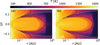 |
Fig. B.3 Temperature map of the model MREF (panel a) and MREF* (panel b) at the respective times at which the MRI active area has reached its largest extent and the cooling front starts to develop (t = tc). The contour lines are equivalent to the ones shown in Fig. 1. |
References
- Alcalá, J. M., Manara, C. F., Natta, A., et al. 2017, A&A, 600, A20 [NASA ADS] [CrossRef] [EDP Sciences] [Google Scholar]
- Armitage, P. J. 2019, SAAS, 45, 1 [NASA ADS] [CrossRef] [Google Scholar]
- Audard, M., Ábrahám, P., Dunham, M. M., et al. 2014, Protostars and Planets VI, 387 [Google Scholar]
- Bae, J., Hartmann, L., Zhu, Z., & Gammie, C. 2013, ApJ, 764, 141 [NASA ADS] [CrossRef] [Google Scholar]
- Bae, J., Hartmann, L., Zhu, Z., & Nelson, R. P. 2014, ApJ, 795, 61 [NASA ADS] [CrossRef] [Google Scholar]
- Baehr, H. 2023, MNRAS, 523, 3348 [NASA ADS] [CrossRef] [Google Scholar]
- Bai, X. N., & Stone, J. M. 2013, ApJ, 769, 76 [NASA ADS] [CrossRef] [Google Scholar]
- Balbus, S. A., & Hawley, J. F. 1991, ApJ, 376, 214 [Google Scholar]
- Bell, K. R., & Lin, D. N. C. 1994, ApJ, 427, 987 [NASA ADS] [CrossRef] [Google Scholar]
- Brož, M., Chrenko, O., Nesvorný, D., & Dauphas, N. 2021, Nat. Astron., 5, 898 [CrossRef] [Google Scholar]
- Cassen, P., Cassen, & Patrick 2001, M&PS, 36, 671 [Google Scholar]
- Cecil, M., Gehrig, L., & Steiner, D. 2024, A&A, 687, A136 [NASA ADS] [CrossRef] [EDP Sciences] [Google Scholar]
- Chambers, J. 2024, ApJ, 966, 40 [NASA ADS] [CrossRef] [Google Scholar]
- Chatterjee, S., & Tan, J. C. 2014, ApJ, 780, 53 [Google Scholar]
- Chrenko, O., Chametla, R. O., Nesvorný, D., & Flock, M. 2022, A&A, 666, A63 [NASA ADS] [CrossRef] [EDP Sciences] [Google Scholar]
- Cleaver, J., Hartmann, L., & Bae, J. 2023, MNRAS, 523, 5522 [NASA ADS] [CrossRef] [Google Scholar]
- Coleman, M. S., Kotko, I., Blaes, O., Lasota, J. P., & Hirose, S. 2016, MNRAS, 462, 3710 [NASA ADS] [CrossRef] [Google Scholar]
- Colmenares, M. J., Lambrechts, M., van Kooten, E., & Johansen, A. 2024, A&A, 685, A114 [NASA ADS] [CrossRef] [EDP Sciences] [Google Scholar]
- Connelly, J. N., Bizzarro, M., Krot, A. N., et al. 2012, Science, 338, 651 [Google Scholar]
- Cui, C., & Bai, X.-N. 2022, MNRAS, 516, 4660 [NASA ADS] [CrossRef] [Google Scholar]
- Desch, S. J., & Turner, N. J. 2015, ApJ, 811, 156 [NASA ADS] [CrossRef] [Google Scholar]
- Drazkowska, J., Stammler, S. M., & Birnstiel, T. 2021, A&A, 647, A15 [EDP Sciences] [Google Scholar]
- Dzyurkevich, N., Turner, N. J., Henning, T., & Kley, W. 2013, ApJ, 765, 114 [NASA ADS] [CrossRef] [Google Scholar]
- Faure, J., & Nelson, R. P. 2016, A&A, 586, A105 [NASA ADS] [CrossRef] [EDP Sciences] [Google Scholar]
- Faure, J., Fromang, S., & Latter, H. 2014, A&A, 564, A22 [NASA ADS] [CrossRef] [EDP Sciences] [Google Scholar]
- Fiorellino, E., Manara, C. F., Nisini, B., et al. 2021, A&A, 650, A43 [NASA ADS] [CrossRef] [EDP Sciences] [Google Scholar]
- Flock, M., & Mignone, A. 2021, A&A, 650, A119 [NASA ADS] [CrossRef] [EDP Sciences] [Google Scholar]
- Flock, M., Fromang, S., González, M., & Commerçon, B. 2013, A&A, 560, A43 [NASA ADS] [CrossRef] [EDP Sciences] [Google Scholar]
- Flock, M., Fromang, S., Turner, N. J., & Benisty, M. 2016, ApJ, 827, 144 [CrossRef] [Google Scholar]
- Flock, M., Fromang, S., Turner, N. J., & Benisty, M. 2017a, ApJ, 835, 230 [CrossRef] [Google Scholar]
- Flock, M., Nelson, R. P., Turner, N. J., et al. 2017b, ApJ, 850, 131 [Google Scholar]
- Flock, M., Turner, N. J., Mulders, G. D., et al. 2019, A&A, 630, A147 [NASA ADS] [CrossRef] [EDP Sciences] [Google Scholar]
- Gerbig, K., Murray-Clay, R. A., Klahr, H., & Baehr, H. 2020, ApJ, 895, 91 [CrossRef] [Google Scholar]
- Hameury, J. M. 2020, ASR, 66, 1004 [Google Scholar]
- Hartmann, L., Herczeg, G., Calvet, N., et al. 2016, ARA&A, 54, 135 [NASA ADS] [CrossRef] [Google Scholar]
- Held, L. E., & Latter, H. N. 2022, MNRAS, 510, 146 [Google Scholar]
- Herbig, G. H. 1977, ApJ, 217, 693 [NASA ADS] [CrossRef] [Google Scholar]
- Hirose, S., Krolik, J. H., & Blaes, O. 2009, ApJ, 691, 16 [NASA ADS] [CrossRef] [Google Scholar]
- Isella, A., & Natta, A. 2005, A&A, 438, 899 [NASA ADS] [CrossRef] [EDP Sciences] [Google Scholar]
- Jang, H., Liu, B., & Johansen, A. 2022, A&A, 664, A86 [NASA ADS] [CrossRef] [EDP Sciences] [Google Scholar]
- Jankovic, M. R., Owen, J. E., Mohanty, S., & Tan, J. C. 2021, MNRAS, 504, 280 [NASA ADS] [CrossRef] [Google Scholar]
- Johansen, A., Klahr, H., Henning, T., et al. 2006, ApJ, 636, 1121 [NASA ADS] [CrossRef] [Google Scholar]
- Johns-Krull, C. M. 2007, ApJ, 664, 975 [Google Scholar]
- Jones, R. H., Villeneuve, J., & Libourel, G. 2018, Crpd, 57 [Google Scholar]
- Kadam, K., Vorobyov, E., & Basu, S. 2022, MNRAS, 516, 4448 [NASA ADS] [CrossRef] [Google Scholar]
- Kama, M., Min, M., & Dominik, C. 2009, A&A, 506, 1199 [NASA ADS] [CrossRef] [EDP Sciences] [Google Scholar]
- Kley, W., Lin, D. N. C., Kley, W., & Lin, D. N. C. 1999, ApJ, 518, 833 [NASA ADS] [CrossRef] [Google Scholar]
- Kóspál, Ábrahám, P., Acosta-Pulido, J. A., et al. 2016, A&A, 596, A52 [NASA ADS] [CrossRef] [EDP Sciences] [Google Scholar]
- Königl, A., Romanova, M. M., & Lovelace, R. V. E. 2011, MNRAS, 416, 757 [NASA ADS] [Google Scholar]
- Lambrechts, M., & Johansen, A. 2014, A&A, 572, A107 [NASA ADS] [CrossRef] [EDP Sciences] [Google Scholar]
- Lasota, J. P. 2001, New Astron. Rev., 45, 449 [CrossRef] [Google Scholar]
- Lee, E. J., Fuentes, J. R., & Hopkins, P. F. 2022, ApJ, 937, 95 [CrossRef] [Google Scholar]
- Lehmann, M., & Lin, M. K. 2022, A&A, 658, A156 [NASA ADS] [CrossRef] [EDP Sciences] [Google Scholar]
- Lesur, G., Flock, M., Ercolano, B., et al. 2023, ASPC, 534, 465 [NASA ADS] [Google Scholar]
- Levermore, C. D., & Pomraning, G. C. 1981, ApJ, 248, 321 [NASA ADS] [CrossRef] [Google Scholar]
- Li, R., Chen, Y. X., & Lin, D. N. 2022, MNRAS, 510, 5246 [NASA ADS] [CrossRef] [Google Scholar]
- Libourel, G., & Portail, M. 2018, SciA, 4, eaar3321 [NASA ADS] [Google Scholar]
- Lin, D. N. C., Papaloizou, J., Faulkner, J., et al. 1985, MNRAS, 212, 105 [NASA ADS] [CrossRef] [Google Scholar]
- Liu, H., Herczeg, G. J., Johnstone, D., et al. 2022, ApJ, 936, 152 [NASA ADS] [CrossRef] [Google Scholar]
- Lyra, W., & Umurhan, O. M. 2019, PASP, 131, 072001 [Google Scholar]
- Macfarlane, B., Stamatellos, D., Johnstone, D., et al. 2019, MNRAS, 487, 5106 [NASA ADS] [CrossRef] [Google Scholar]
- Malygin, M. G., Kuiper, R., Klahr, H., Dullemond, C. P., & Henning, T. 2014, A&A, 568, A91 [NASA ADS] [CrossRef] [EDP Sciences] [Google Scholar]
- Manara, C. F., Testi, L., Herczeg, G. J., et al. 2017, A&A, 604, A127 [NASA ADS] [CrossRef] [EDP Sciences] [Google Scholar]
- Martin, R. G., & Lubow, S. H. 2011, ApJ, 740, L6 [NASA ADS] [CrossRef] [Google Scholar]
- Mignone, A., Bodo, G., Massaglia, S., et al. 2007, ApJS, 170, 228 [Google Scholar]
- Mohanty, S., Jankovic, M. R., Tan, J. C., & Owen, J. E. 2018, ApJ, 861, 144 [Google Scholar]
- Mulders, G. D., Pascucci, I., & Apai, D. 2015, ApJ, 798, 112 [Google Scholar]
- Mulders, G. D., Pascucci, I., Apai, D., & Ciesla, F. J. 2018, AJ, 156, 24 [Google Scholar]
- Nayakshin, S., de Miera, F. C. S., Ágnes Kóspál, et al. 2024, MNRAS, 530, 1749 [NASA ADS] [CrossRef] [Google Scholar]
- Pavlyuchenkov, Y. N., Akimkin, V. V., Topchieva, A. P., & Vorobyov, E. I. 2023, ARep, 67, 470 [NASA ADS] [Google Scholar]
- Petigura, E. A., Marcy, G. W., Winn, J. N., et al. 2018, AJ, 155, 89 [Google Scholar]
- Rab, C., Elbakyan, V., Vorobyov, E., et al. 2017, A&A, 604, A15 [NASA ADS] [CrossRef] [EDP Sciences] [Google Scholar]
- Rea, D. G., Simon, J. B., Carrera, D., et al. 2024, ApJ, 972, 128 [NASA ADS] [CrossRef] [Google Scholar]
- Romanova, M. M., & Owocki, S. P. 2015, Space Sci. Rev., 191, 339 [Google Scholar]
- Romanova, M. M., Blinova, A. A., Ustyugova, G. V., Koldoba, A. V., & Lovelace, R. V. 2018, NewA, 62, 94 [CrossRef] [Google Scholar]
- Ross, J., Latter, H. N., Tehranchi, M., et al. 2017, MNRAS, 468, 2401 [NASA ADS] [CrossRef] [Google Scholar]
- Schobert, B. N., Peeters, A. G., & Rath, F. 2019, ApJ, 881, 56 [NASA ADS] [CrossRef] [Google Scholar]
- Scott, E. R. D. 2007, AREPS, 35, 577 [NASA ADS] [Google Scholar]
- Shakura, N. I., & Sunyaev, R. A. 1973, A&A, 24, 337 [NASA ADS] [Google Scholar]
- Simon, J. B., Armitage, P. J., Li, R., & Youdin, A. N. 2016, ApJ, 822, 55 [Google Scholar]
- Simon, J. B., Bai, X.-N., Flaherty, K. M., & Hughes, A. M. 2018, ApJ, 865, 10 [NASA ADS] [CrossRef] [Google Scholar]
- Steiner, D., Gehrig, L., Ratschiner, B., et al. 2021, A&A, 655, A110 [NASA ADS] [CrossRef] [EDP Sciences] [Google Scholar]
- Taki, T., Fujimoto, M., & Ida, S. 2016, A&A, 591, A86 [NASA ADS] [CrossRef] [EDP Sciences] [Google Scholar]
- Toomre, A. 1964, ApJ, 139, 1217 [Google Scholar]
- Trinquier, A., Elliott, T., Ulfbeck, D., et al. 2009, Science, 324, 374 [Google Scholar]
- Tsuchiyama, A., Tachibana, S., & Takahashi, T. 1999, Geochim. Cosmochim. Acta, 63, 2451 [NASA ADS] [CrossRef] [Google Scholar]
- Ueda, T., Okuzumi, S., & Flock, M. 2017, ApJ, 843, 49 [NASA ADS] [CrossRef] [Google Scholar]
- Vorobyov, E. I., & Basu, S. 2006, ApJ, 650, 956 [CrossRef] [Google Scholar]
- Vorobyov, E. I., Skliarevskii, A. M., Molyarova, T., et al. 2022, A&A, 658, A191 [NASA ADS] [CrossRef] [EDP Sciences] [Google Scholar]
- Wunsch, R., Gawryszczak, A., Klahr, H., & Rozyczka, M. 2005, MNRAS, 367, 773 [Google Scholar]
- Yang, C. C., Johansen, A., & Carrera, D. 2017, A&A, 606, A80 [NASA ADS] [CrossRef] [EDP Sciences] [Google Scholar]
- Zhu, Z., Hartmann, L., & Gammie, C. 2009a, ApJ, 694, 1045 [Google Scholar]
- Zhu, Z., Hartmann, L., Gammie, C., & McKinney, J. C. 2009b, ApJ, 701, 620 [CrossRef] [Google Scholar]
- Zhu, Z., Hartmann, L., Gammie, C. F., et al. 2010, ApJ, 713, 1134 [Google Scholar]
The power of 3 in the hyperbolical tangent function is not strictly necessary, but was kept to stay consistent with the description of Flock et al. (2019).
For instance, if the radial velocity, υr, is defined such that positive values correspond to a flow towards larger radii and υr(rout, θ) < 0, then  , with U being the computational domain and
  being its numerical radial outer boundary.
We also tested a lower value of this factor of 0.05 and observed no significant impact on the hydrodynamic evolution.
All Tables
Properties of the TI-induced accretion events occurring in the models MREF and M3. M1 and M2 do not accumulate enough mass to trigger the TI.
All Figures
|
Fig. 1 Temperature (panels a and b) and gas density (panels c and d) maps for the model MREF in the initial configuration at t = t0 and at the end of the quiescent phase, shortly before the TI is triggered, t = tTI − ∆t. Yellow contour lines depict the region of dust sublimation (T = Ts), black lines show the ionisation transition from the MRI active zone to the dead zone (T = TMRI), and green lines mark the radial optical depth τ, = 2/3 surface. In panels c and d, the red contours are drawn at ρgas = 10−9 which corresponds to a dust density of ρdust = 10−12. |
| In the text | |
|
Fig. 2 Surface density profiles of models with different Ṁint at distinct evolutionary stages. Panel a shows the initial configuration for all models, while panel b presents their structure after the first TI and the subsequent diffusion of the resulting density bumps. Panel c compares the surface density of MREF and M3 at the start of their respective second TI cycle, and panel d shows the structure of both models after they have become quiescent again (similar to panel b). In all cases, the TI phase persists until enough mass has been accreted so that the surface density does not exceed Σcut. |
| In the text | |
|
Fig. 3 Evolution of the accretion rate (panel a) and the position of the dead zone inner edge at the midplane (panel b) for the four different models analysed in this work. Panels a1 and b1 show a zoom-in to the time frame in which the TI-induced accretion event is occurring in the MREF model. The vertical dashed lines in panel a1 indicate the times corresponding to the ignition of the TI (tTI), the heating front reaching its largest extent and a cooling front starting to develop (tc), the retreat of the cooling front towards the star (tret) and the ignition of the first reflare (trefl). In panel a, the vertical dashed lines mark the points in time for which the surface profiles of the MREF model in panels b (tcut1 ) and d (tcut2) of Fig. 2 are shown. |
| In the text | |
|
Fig. 4 Temperature maps (upper row) and corresponding surface density profiles (lower row) for four snapshots in time during an outburst event. In the upper row, the black contour lines correspond to T = TMRI, the yellow ones to T = TS, and the green ones to a radial optical depth of τ* = 2/3. tTI is chosen to be the point in time at which the TI is triggered. The second column shows the state of the disc at the time the MRI active region has reached its largest extent during the main burst (tc). The third column represents the stage of the ignition of the first reflare (trefl), the maximum extent of which is reached at the time depicted in column four. The state of the disc shortly after the instability has ended is shown in column five. |
| In the text | |
|
Fig. 5 Midplane temperature profiles of the MREF and M3 models at the time of the onset of the TI (tTI) and at the time at which the cooling front develops (tc). |
| In the text | |
|
Fig. 6 Space-time diagrams of MREF (panel a), M3 (panel b) and M2 (panel c) with the colours corresponding to the surface density at the respective locations and times. While a TI cycle develops within a 3000 yr time frame in the MREF and M3, the M2 model does not show signs of TI even after about 5000 yr and the disc has reached a quasi-steady state. The white contours indicate the positions of pressure maxima. Panel a1 shows the space-time diagram of the TI phase of the MREF model. The cyan contour line corresponds to the location of the inner edge of the dead zone at the midplane. |
| In the text | |
|
Fig. 7 S-curve of the MREF model at a radius of 0.2 AU. The black line corresponds to the evolutionary track during the quiescent phase, while the coloured dots are taken from snapshots during the outburst stage. The red data points were extracted during the first outburst and the yellow, green and blue dots make up the evolutionary tracks during the first, second and third reflare, respectively. The density of the dots along an evolutionary track indicates the velocity at which the disc evolves. The arrows are exemplary for the first two cycles and indicate the direction in which the model evolves. The surface density value at which the disc switches from the upper branch (where α = αMRI) to the lower branch (where α = αDZ) is the same for each cycle and is marked with |
| In the text | |
|
Fig. 8 Surface density profiles of the models MREF and M3 for three points in time each. tc, tret and trefl correspond to the points in time described in Fig. 3. The fit for the minimum values of the surface density valley travelling alongside the cooling front |
| In the text | |
|
Fig. 9 S-curves during a TI-induced accretion event for the MREF model with (panel a) and without (panel b) the effect of irradiation heating, calculated at the respective radii at which the reflares are ignited. These radii are 0.091 AU and 0.087 AU for panel a and panel b, respectively. The data points with red, yellow, green, blue and pink colours were taken during the first, second, third, fourth and fifth reflare, respectively. With irradiation heating, the later reflares are ignited at smaller surface densities than the first three. The different critical surface density values are marked with |
| In the text | |
|
Fig. 10 Radial proflies of the surface density (panel a), the temperature (panel b) and the pressure scale height (panel c) within 1 AU for one representative point in time each during the TI development in the MREF* and M3* models. In panel a, dashed lines represent the gas surface density, Σg, solid lines show the dust surface density, Σd, and the dotted lines depict the respective fits to the dust surface density, Σd,fit, in the high-state region, evaluated with Eq. (25). Σd and Ed,fit are multiplied by 1000 to compensate for the baseline dust-to-gas mass ratio ƒ0 and make the values comparable to Σg. The solid lines in panel b correspond to the midplane temperature, while the dashed lines represent the dust sublimation temperature. |
| In the text | |
|
Fig. 11 Evolution of the midplane temperature (panel a) and midplane total gas pressure (panel b) at the location of the pebble trap (at 0.15 AU) during a TI-induced accretion event. |
| In the text | |
|
Fig. A.1 Visualisation of the Rosseland mean gas opacity coefficients given by Malygin et al. (2014). The dashed white rectangle indicates the density- and temperature regions for the gas from which the average value implemented in our simulations has been extracted. |
| In the text | |
|
Fig. B.1 Schematic visualisation of the functions describing the dust-to-gas mass ratio in the MREF and MREF* models. For illustrative purposes, the density was held constant, representative profiles for the temperature and radial optical depth have been chosen and the models are shown as functions of a dimensionless radius. The vertical dashed black lines mark locations where the temperature crosses the dust sublimation temperature. |
| In the text | |
|
Fig. B.2 Evolution of the accretion rate (panel a) and the position of the dead zone inner edge at the midplane (panel b) during TI-induced accretion events in the models MREF and MREF*. |
| In the text | |
|
Fig. B.3 Temperature map of the model MREF (panel a) and MREF* (panel b) at the respective times at which the MRI active area has reached its largest extent and the cooling front starts to develop (t = tc). The contour lines are equivalent to the ones shown in Fig. 1. |
| In the text | |
Current usage metrics show cumulative count of Article Views (full-text article views including HTML views, PDF and ePub downloads, according to the available data) and Abstracts Views on Vision4Press platform.
Data correspond to usage on the plateform after 2015. The current usage metrics is available 48-96 hours after online publication and is updated daily on week days.
Initial download of the metrics may take a while.