| Issue |
A&A
Volume 692, December 2024
|
|
|---|---|---|
| Article Number | A256 | |
| Number of page(s) | 12 | |
| Section | Stellar structure and evolution | |
| DOI | https://doi.org/10.1051/0004-6361/202451758 | |
| Published online | 17 December 2024 | |
The role of thermal instability in accretion outbursts in high-mass stars
1
Fakultät für Physik, Universität Duisburg-Essen, Lotharstraße 1, D-47057 Duisburg, Germany
2
School of Physics and Astronomy, University of Leicester, Leicester LE1 7RH, UK
3
INAF-Osservatorio Astronomico di Capodimonte, Salita Moiariello 16, 80131 Napoli, Italy
4
Instituto de Física y Astronomía, Universidad de Valparaíso, Ave. Gran Bretaña, 1111, Casilla, 5030 Valparaíso, Chile
5
Centre for Astrophysics, University of Hertfordshire, College Lane Hatfield AL10 9AB, UK
6
Millennium Institute of Astrophysics, Nuncio Monseñor Sotero Sanz 100, Of. 104, Providencia, Santiago, Chile
⋆ Corresponding author; This email address is being protected from spambots. You need JavaScript enabled to view it.
Received:
1
August
2024
Accepted:
8
November
2024
Abstract
Context. High-mass young stellar objects (HMYSOs) can exhibit episodic bursts of accretion, accompanied by intense outflows and luminosity variations. Understanding the underlying mechanisms driving these phenomena is crucial for elucidating the early evolution of massive stars and their feedback on star formation processes.
Aims. Thermal instability (TI) due to hydrogen ionisation is among the most promising mechanisms of episodic accretion in low-mass (M* ≲ 1 M⊙) protostars. Its role in HMYSOs has not yet been determined. Here we investigate the properties of TI outbursts in young massive (M* ≳ 5 M⊙) stars, and compare them to those that have been observed to date.
Methods. We employed a 1D numerical model to simulate TI outbursts in HMYSO accretion discs. We varied the key model parameters, such as stellar mass, mass accretion rate onto the disc, and disc viscosity, to assess the TI outburst properties.
Results. Our simulations show that modelled TI bursts can replicate the durations and peak accretion rates of long outbursts (a few years to decades) observed in HMYSOs with similar mass characteristics. However, they struggle with short-duration bursts (less than a year) with short rise times (a few weeks or months), suggesting the need for alternative mechanisms. Moreover, while our models match the durations of longer bursts, they fail to reproduce the multiple outbursts seen in some HMYSOs, regardless of model parameters. We also emphasise the significance of not just evaluating model accretion rates and durations, but also performing photometric analysis to thoroughly evaluate the consistency between model predictions and observational data.
Conclusions. Our findings suggest that some other plausible mechanisms, such as gravitational instabilities and disc fragmentation, can be responsible for generating the observed outburst phenomena in HMYSOs, and we underscore the need for further investigation into alternative mechanisms driving short outbursts. However, the physics of TI is crucial in sculpting the inner disc physics in the early bright epoch of massive star formation, and comprehensive parameter space exploration; the use of 2D modelling is essential to obtaining a more detailed understanding of the underlying physical processes. By bridging theoretical predictions with observational constraints, this study contributes to advancing our knowledge of HMYSO accretion physics and the early evolution of massive stars.
Key words: hydrodynamics / instabilities / protoplanetary disks / stars: formation
© The Authors 2024
 Open Access article, published by EDP Sciences, under the terms of the Creative Commons Attribution License (https://creativecommons.org/licenses/by/4.0), which permits unrestricted use, distribution, and reproduction in any medium, provided the original work is properly cited.
This article is published in open access under the Subscribe to Open model. This email address is being protected from spambots. You need JavaScript enabled to view it. to support open access publication.
1. Introduction
Understanding the formation and evolution of high-mass young stellar objects (HMYSOs), and their various accretion outbursts, requires a comprehensive study that includes observations, analytical models, and numerical simulations. HMYSOs hold crucial information on the formation processes of massive stars, which play a key role in shaping the cosmic environment. While FU Orionis-type accretion outbursts are typically associated with low-mass young stellar objects (YSOs) (Hartmann & Kenyon 1996), recent observations have suggested that HMYSOs may also experience similar episodic accretion events (Caratti o Garatti et al. 2017; Stecklum et al. 2021; Fischer et al. 2023). However, the mechanisms driving these outbursts in HMYSOs are likely different, given the distinct physical conditions in high-mass star formation.
FU Orionis-type accretion outbursts are a puzzling and fascinating phenomenon in astrophysics, primarily observed in low-mass YSOs. These outbursts, which last for several years or decades, involve an intense increase in the accretion rate onto a young star, leading to a brightening of several magnitudes. The prototype of this class of outbursts is FU Orionis itself, a low-mass star discovered more than 85 years ago (Herbig 1977). Since then, many other examples of FUors have been identified in different regions of our galaxy (Audard et al. 2014), providing evidence that these phenomena might be ubiquitous in low-mass star-forming environments. Later on, with the discovery of EXor bursts (Herbig 1989), it was realised that episodic accretion is a much broader and varied phenomenon that occurs at all stages of star formation. The outburst of V1647 Ori in 2004 showed that some objects do not fit into the traditional EXor and FUor categories, despite the broad range of properties these groups cover. Properties of several recently discovered outbursting objects are even more unusual, thus creating a zoo of outbursting objects with various properties (see Fischer et al. 2023, for the review).
Despite several attempts to explain the physical processes driving these outbursts, the exact mechanism behind them remains unclear. Nevertheless, numerous theoretical scenarios have been proposed, ranging from gravitational instability (GI) in the disc around the young star (Vorobyov & Basu 2010; Machida et al. 2011; Hosokawa et al. 2016; Meyer et al. 2017; Vorobyov & Elbakyan 2018; Zhao et al. 2018; Kuffmeier et al. 2018; Oliva & Kuiper 2020), thermal instability (TI) (Bell & Lin 1994; Kley & Lin 1996), stellar flyby (Borchert et al. 2022; Cuello et al. 2023), interaction of a massive planet with the disc (Lodato & Clarke 2004), or the presence of a ‘dead zone’ in the inner 0.1 ≤ r ≤ a few AU disc with the eventual development of the magnetorotational instability (MRI) in that zone (Armitage et al. 2001; Zhu et al. 2009, 2010; Kadam et al. 2020; Vorobyov et al. 2020).
One of the possible mechanisms responsible for the episodic accretion outbursts is the well-established phenomenon of disc thermal instability caused by the sudden increase in opacity when hydrogen ionises at a temperature of ∼104 K. The inner thermally unstable region of the disc periodically switches between two stable branches (cold and hot) of the S-curve (see Sect. 6 in Armitage 2015), thus developing a strong accretion variability onto the star (e.g. Lodato & Clarke 2004; Elbakyan et al. 2021). This phenomenon was originally studied as part of a model for dwarf novae (Hōshi 1979; Meyer & Meyer-Hofmeister 1981; Lin et al. 1985). This model, while proving to be a good fit to the observations, requires a substantial change in opacity and distinct values of the α-parameter for the cold and hot branches of the S-curve, and also requires that the disc midplane temperatures exceed ∼104 K.
The initial studies of accretion outbursts focused mainly on FU Orionis objects (FUors), which are low-mass stars exhibiting outbursts every few decades (Hartmann & Kenyon 1996). However, with the advent of observational techniques and new instruments (e.g. ALMA, VLTI, VISTA), several groups have discovered multiple HMYSOs showing accretion outbursts (Caratti o Garatti et al. 2017; Hunter et al. 2018; Stecklum et al. 2021; Chen et al. 2021; Wolf et al. 2024), which introduce some discrepancies among their observational properties compared to the FUors. These discrepancies could potentially help to fill in critical details of the underlying physical mechanisms at work, as well as refining theoretical predictions. While in low-mass YSOs we distinguish the two large categories as magnetospheric-accretion driven (EXors) and boundary layer accretion driven (FUors), in HMYSOs the situation is more complex as, in principle, magnetospheric accretion should not work (Beltrán & de Wit 2016; Mendigutía 2020). The outbursts so far observed in HMYSOs are rapid and short-lived events that are manifested by a sudden increase in luminosity that may last from months to a few decades before returning to quiescence. Unfortunately, due to the low statistics for the outbursts in HMYSOs (fewer than ten objects), it is hard to determine their recurrent rate, as was done for FUors (∼1.75 kyr; Contreras Peña et al. 2024). It is worth noting that bursts similar to the one in the FU Orionis system have not yet been detected in HMYSOs; all the bursts observed to date have relatively short durations and low amplitudes compared to the FU Ori bursts. However, the lack of detections is likely due to an observational bias (and the relative small number of such events); we should keep an open mind and ask ourselves if FUor events are possible in HMYSOs. While the observed sample is still too small to judge whether these short bursts represent a common and unique feature or are just caused by an observational bias, we can still draw some conclusions.
The short durations of the bursts correspond to the dynamical and viscous timescales at the (sub-)AU radial distances, meaning that only the region of the disc close to the star is involved in the burst triggering. However, the multi-dimensional numerical simulation of (sub-)AU radial distances in a disc is usually too computationally costly and a sink cell approach is used to simulate the inner region of the disc (Meyer et al. 2017; Oliva & Kuiper 2020) or these small-scale structures are hidden within a Gaussian accretion kernel around sink particles (Krumholz et al. 2004; Mignon-Risse et al. 2020; Commerçon et al. 2022). This approach does not allow the hydrodynamical evolution of the inner disc to be simulated properly, which is crucial for the understanding of accretion outbursts. The most practical way to overcome this computational barrier is to use one-dimensional (1D) numerical models of circumstellar discs.
In our current study, our aim is to advance our understanding of accretion outbursts in HMYSOs by investigating the main characteristics of the phenomenon and its fundamental effects on forming massive stars and their surrounding discs. This is done by studying the evolution of circumstellar discs around HMYSOs, which are prone to TI in the inner disc.
In Sect. 2 we detail the numerical methodology employed in this study. We discuss the implementation of classic thermal instability (TI) bursts in Sect. 3, where we explore the fundamental characteristics of these bursts under varying model parameters. In Sect. 4 we extend our analysis to investigate TI bursts for different sets of model parameters, systematically examining their impact on the observed burst behaviour of HMYSOs. Following this, in Sect. 5 we compare our simulation results with observational data. In Sect. 6 we delve into the phenomenon of thermal instability bursts with higher frequency. The discussion section (Sect. 7) covers comparisons with observational data, possible burst mechanisms, and the importance of parameter space exploration. We conclude with our main findings and suggestions for future research in Sect. 8.
2. Numerical methodology
The evolution of the protoplanetary disc is simulated using a 1D Shakura-Sunyaev viscous disc model (Shakura & Sunyaev 1973), implemented in the hydrodynamical code DEO, with azimuthal symmetry and vertical averaging (Nayakshin & Lodato 2012; Elbakyan et al. 2021; Nayakshin et al. 2022). The detailed description of the DEO model can be found in Nayakshin & Elbakyan (2024); here we present only the modified model properties. The master equation for the viscous evolution can be presented as
![Mathematical equation: $$ \begin{aligned} \frac{\partial \Sigma }{\partial t} =&\frac{3}{r} \frac{\partial }{\partial r} \left[r^{1/2} \frac{\partial }{\partial r} \left(r^{1/2}\nu \Sigma \right)\right]\nonumber \\&+\frac{\dot{M}_{\mathrm{dep} }}{2\pi ^{3/2} r \sigma } \exp \left[-\left(\frac{r-r_{\mathrm{dep} }}{\sigma }\right)^2\right], \end{aligned} $$](/articles/aa/full_html/2024/12/aa51758-24/aa51758-24-eq1.gif) (1)
(1)
where Σ is the gas surface density, ν is the kinematic viscosity of the disc, and the last term on the right-hand side is responsible for the mass deposition from outer regions into the disc. The mass is deposited from the envelope into the disc at a constant rate, Ṁdep, in a Gaussian ring with a centroid radius rdep = 18 AU and dispersion σ = 0.05 rdep. Our computational grid is logarithmic, with 124 default radial zones covering the radial region from Rin = 0.1 AU to 20 AU. The disc in our model is initially in a steady-state configuration, with an accretion rate Ṁ = Ṁdep at all disc radii.
In our models we simulate only the inner 20 AU of the disc, while the observed disc sizes around HMYSOs typically range from a few hundred to a few thousand AU (Beltrán & de Wit 2016). Our simulated discs have masses ranging from a few times 10−1 M⊙ to a few M⊙, depending on the stellar mass, consistent with observations of circumstellar discs in HMYSOs (e.g. Cesaroni et al. 2006). This results in disc-to-star mass ratios greater than 0.1, which aligns with observational findings (e.g. Ahmadi et al. 2023).
We parametrise the kinematic viscosity in the disc through the dimensionless α-parameter, ν = αcsH (Shakura & Sunyaev 1973), where cs is the gas sound speed in the disc midplane and H is the vertical scale height of the disc. Following Hameury et al. (1998), we define the α-parameter as
 (2)
(2)
where Tcr is a critical temperature (see below), αcold and αhot are α-parameters on the cold and hot branches of the S-curve. Recent magnetohydrodynamic (MHD) simulations suggest αcold ≈ 10−2, while there is a large discrepancy for the values of αhot. Most of the global disc simulations adopt a magnetic field geometry that is similar to zero net-flux shearing-box and produce values of αhot ∼ 0.01 − 0.02 (Miller & Stone 2000; Hirose et al. 2006; Fromang & Nelson 2006; Shi et al. 2010; Davis et al. 2010; Flock et al. 2011; Beckwith et al. 2011; Simon et al. 2012). Meanwhile, the value of αhot estimated from the observations of dwarf novae and X-ray binaries, found to be of the order of 0.1 (Smak 1999; Dubus et al. 2001). It is therefore questioned how correct it is to use zero mean field models for simulations of accretion discs (see discussions in King et al. 2007; Zhu et al. 2009; Bai & Stone 2013). Recent 3D MHD models show that the joint action of convection and magnetorotational instability can increase αhot to the observational values (Hirose et al. 2014; Coleman et al. 2018; Scepi et al. 2018). The values of αcold = 0.01 and αhot = 0.1 were found to work relatively well for both observations (e.g. Lasota 2001) and first-principle simulations of TI in discs (e.g. Hirose et al. 2014).
Thermal equilibrium in protoplanetary discs is crucial for understanding the temperature distribution and physical conditions within these discs. It relies on the equilibrium between the heating and cooling processes within the disc’s vertical structure. In our previous works (Nayakshin et al. 2023; Elbakyan et al. 2023; Nayakshin & Elbakyan 2024) we used a time-dependent energy balance equation with a one-zone approximation for the vertical thermal equilibrium and a radial advection of the heat (Lodato & Clarke 2004; Nayakshin & Lodato 2012). This approach is a useful tool for providing a simplified overview of the thermal balance in protoplanetary discs. However, it should be used with caution and with an awareness of its limitations.
For a more accurate representation of the complex physical processes occurring in discs, we improved the energy balance equation in our model, following Cannizzo (1993) and Menou et al. (1999). Instead of the one-zone approximation in the vertical direction, we solved the z-dependent vertical balance equations (cf. Sect. 2.3 in Nayakshin et al. 2024)
 (3)
(3)
where P(z) and ρ(z) are the local gas pressure and density, respectively. We find P for a given ρ and T, where the temperature T satisfies the equation
 (4)
(4)
where
 (5)
(5)
Here z2/3 is the location of the τ(z) = 2/3 surface with the temperature T(z) = Teff.
The disc temperature evolves as
 (6)
(6)
where tth is the thermal timescale, vr is the radial velocity, and Teq is the equilibrium temperature in the disc at the radial distance r, found from the assumption of the vertical energy balance for the disc. In the one-zone approximation it is assumed that the opacity κ in the disc is the same at the midplane and at its surface. However, κ strongly depends on the temperature in the disc, which can vary by up to an order of magnitude between the midplane and the disc surface. The z-dependent vertical balance equations eliminate the need to assume that κ in the disc is the same in the vertical direction. In our model, we use opacities from Zhu et al. (2009). A more detailed description of the model can be found in Nayakshin et al. (2024). For the models presented in this section, we set Tcr = 8000 K, unlike the Tcr = 2.5 × 10⁴ K used for the one-zone models earlier. The reasons for these choices are discussed in Sect. 6.
3. Classic thermal instability bursts
In this section we discuss the classic thermal instability (TI) bursts in HMYSO discs. We establish their main characteristics, such as the mass accretion rate during the burst, its rise time, and duration. We also explore how the parameters of the problem, such as M*, viscosity parameter in the hot state (αhot), and feeding rate, affect the observability of the bursts.
We start by considering and briefly describing one thermal instability cycle for a model with M* = 10 M⊙, Ṁdep = 10−4 M⊙ yr−1, and the value of αcold = 0.01 and αhot = 0.1. The solid black curve in the bottom panel of Fig. 1 shows the mass accretion rate onto the star versus time for this model. The top four panels of Fig. 1 present the radial profiles of key disc variables (surface density Σ, midplane temperature, effective temperature, and disc aspect ratio H/r) at five distinct time instances indicated with the corresponding vertical lines in the bottom panel. The time t = 0 corresponds to the very beginning of the burst. As is well known, classic TI bursts are triggered very close to the disc inner boundary and propagate outward (e.g. Bell & Lin 1994). This is born out by our models: the temperature jumps to the hot stable branch at r ≈ 0.14 AU first, where hydrogen becomes ionised. The ionisation front then propagates both inward and outward. The inward propagating front produces the Ṁ ≈ 10−3 M⊙ yr−1 burst onto the star, with the rise time of ≈0.1 yr, which is sustained for less than a year (a fraction of the local viscous time). Subsequently, the ionisation front propagating outward puts the disc onto the hot stable branch at increasingly larger radii, but Ṁ∗ decreases monotonically with time. Eventually, the front stalls at rTI ≈ 2 AU and then retreats back as the disc falls into quiescence once again. The value of rTI can be found semi-analytically as (Bell & Lin 1994; Nayakshin et al. 2024)
 (7)
(7)
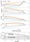 |
Fig. 1. Evolution of disc properties and mass accretion rate during a thermal instability outburst. Top four panels: Radial profiles of gas surface density (top panel), midplane disc temperature (second panel), effective disc temperature (third panel), and disc aspect ratio (fourth panel) for five distinct time instances. Bottom panel: Mass accretion rate history onto the HMYSO during the TI outburst. The vertical dashed lines indicate the time instances for which the radial profiles with corresponding colours are shown in the top panels. The horizontal dashed line shows the value of Ṁth calculated with Eq. (8). The shaded area shows the non-observable part of the accretion rate variations. |
Thus, the region of the disc influenced by thermal instability is limited to where the effective temperature in the steady-state disc exceeds approximately 2000 K. As shown in the fourth panel of Fig. 1, our model aligns well with this analytical estimate, with the ionisation front halting roughly at the point where the disc’s effective temperature falls below 2000 K.
Due to the inside-out propagation of the ionisation front, a region with increased density and temperature forms at the location where the front stalls. If the density/temperature in this region becomes critical and triggers TI, a new reflare will be initiated at this location of the disc (Menou et al. 2000; Dubus et al. 2001). We discuss models with reflares in Sect. 6.2. At the end of the outburst, the surface density profile of the disc does not recover its pre-burst configuration (compare the dark blue and light blue curves in the top panel). This is due to the disc being emptied out onto the star during the burst. The next outburst will repeat only when the inner disc region is resupplied with fresh material from outside. The duration of the burst is of the order of the disc viscous time at the outer radius of the ionised zone, tvisc = rTI2/ν.
One important observational difference between TI outbursts on low-mass and high-mass stars is that the latter are orders of magnitude brighter than the former. TI outbursts must outshine the star to be observationally important. A crude but useful precondition for a burst to be observable is for the bolometric accretion luminosity, Lacc = GM∗ Ṁ∗/R/R∗, to exceed the pre-burst luminosity of the central star, L*. We hence introduce the threshold value Ṁth, and assume that a TI burst is observable when the mass accretion rate onto the star is higher than this threshold value, defined as
 (8)
(8)
where L* = 1.4(M*/M⊙)3.5 L⊙ is the stellar luminosity, R* = (M*/M⊙)0.7 R⊙ is the stellar radius and M* is the stellar mass. Here we used mass-luminosity and mass-radius relations for ZAMS stars, and this threshold value can be considered as a conservative minimum value since the changes of stellar luminosity and radius during the intensive mass accretion are neglected. During accretion outbursts, with high accretion rates of Ṁ∗ > 10−4 M⊙ yr−1, the radius of a HMYSO can change dramatically, reaching a few hundred solar radii (Hosokawa & Omukai 2009; Kuiper & Yorke 2013; Tanaka et al. 2017; Meyer et al. 2019), while during more moderate accretion with Ṁ∗ < 10−4 M⊙ yr−1 a star with mass M ≳ 10 M⊙ has a radius close to the ZAMS value. For all our models, to avoid discrepancy and the addition of new free parameters, we set R* ≈ 20 R⊙, which is an intermediate value between the two extreme cases. However, for the calculation of Ṁth, we used the R* ∝ M*0.7 relation since it is a more conservative value and cannot lead to the underestimation of the number of TI bursts or the duration. We plan to conduct a study with the self-consistent evolution of HMYSO radius using a stellar evolution code in the future. The horizontal line in the bottom panel of Fig. 1 shows Ṁth in our model. Below we discuss in detail the burst duration in our model with αhot = 0.1 and discuss the influence of αhot parameter on the burst observability and duration.
4. TI bursts for different model parameters
In Fig. 2 we show the long-term (2500 years) temporal evolution of mass accretion rate onto the HMYSO for three values of stellar mass: M* = 5 M⊙ (top panel), M* = 10 M⊙ (middle panel), and M* = 20 M⊙ (bottom panel). The observed gas infall rates in high-mass star-forming regions are estimated to be in range 10−5 − 10−3 M⊙ yr−1 (Beuther et al. 2013, 2017; Moscadelli et al. 2021). Thus, for each M* we calculated three models with different values of Ṁdep: 3 × 10⁻⁵ M⊙ yr−1 (blue line), 10−4 M⊙ yr−1 (black line), and 3 × 10⁻⁴ M⊙ yr−1 (red line). The threshold Ṁth (Eq. (8)) is shown with the horizontal dashed line. The variability of the accretion rate in the shaded region below that line is not visible. Clearly, the TI bursts for all stellar masses are observable.
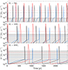 |
Fig. 2. Accretion rate onto the star of mass M* = 5 M⊙ (top panel), M* = 10 M⊙ (middle panel), and M* = 20 M⊙ (bottom panel) during TI bursts for three different values of Ṁdep–3 × 10⁻⁵ M⊙ yr−1 (blue line), 10−4 M⊙ yr−1 (black line), and 3 × 10⁻⁴ M⊙ yr−1 (red line). The horizontal black dashed line shows the Ṁth value for each stellar mass calculated with Eq. (8). The accretion rate variability below the dashed line (shaded region) is unlikely to be observable. The horizontal dotted lines show the Ṁdep for each model with the corresponding colour. The time instance t = 0 in all panels of the figure is arbitrary. |
Figure 2 demonstrates that TI burst duration, amplitude, and repetition timescale, trep, all depend on Ṁdep. We find that trep increases with M*, being on average ∼300 years for the M* = 5 M⊙ model, ∼450 years for the M* = 10 M⊙ model, and ∼850 years for the M* = 20 M⊙ model. This implies that classical TI bursts could happen multiple times on the HMYSOs during their formation timescale of a few ×105 yr (Sabatini et al. 2021). It is interesting to note that even with fewer than ten HMYSO bursts observed to date (cf. Sect. 5), there are objects with multiple bursts, for which trep ∼ 6 − 30 yr. However, there may be physics leading to bursts with far shorter trep (Sect. 6).
In a quasi-steady state, TI bursts are highly periodic and repeatable. Thus, we chose a single TI outburst from each simulation shown in Fig. 2 to study its properties in more detail in Fig. 3.
We first focus on models with M* = 5 M⊙ (top panel). The peak accretion rates during TI bursts for Ṁdep = 3 × 10⁻⁵ M⊙ yr−1 and Ṁdep = 10−4 M⊙ yr−1 are 2 × 10⁻³ M⊙ yr−1 and 3.9 × 10⁻³ M⊙ yr−1, correspondingly. These peak values are comparable to those inferred in observations, Ṁ∗ ≈ 10−3 M⊙ yr−1 (see Table 3). The model with Ṁdep = 3 × 10⁻⁴ M⊙ yr−1 has a peak value of 10−2 M⊙ yr−1, which is one order of magnitude higher than the observed values. All three models show a sharp rise at the beginning of the outburst, which then slows somewhat before the maximum is reached, followed by an even slower decay. The burst rise timescales are somewhat consistent with the observations, being mostly longer. The duration of the observable part of the burst for the Ṁdep = 3 × 10⁻⁵ M⊙ yr−1, Ṁdep = 10−4 M⊙ yr−1, and Ṁdep = 3 × 10⁻⁴ M⊙ yr−1 models are ≈6.2, 13.5, and 31.3 years, respectively, longer than many of the bursts observed so far.
The models for M* = 10 M⊙ and M* = 20 M⊙ are shown in the middle and bottom panels of Fig. 3, respectively. The peak accretion rates during the TI bursts in all three models with M* = 10 M⊙ are slightly higher compared to the M* = 5 M⊙ case, which contributes to longer burst durations. The burst durations are ≈7, 17.8, and 38.2 years for the models with Ṁdep= 3 × 10⁻⁵ M⊙ yr−1, Ṁdep= 10−4 M⊙ yr−1, and Ṁdep= 3 × 10⁻⁴ M⊙ yr−1, respectively. In these cases the longer burst durations are due to the thermal instability being triggered at larger radii in the disc, resulting in a greater portion of the disc contributing to the accretion process. We note that the burst durations are longer, even considering that Ṁth for a M* = 10 M⊙ star is higher than for a M* = 5 M⊙ star.
For the models with a M* = 20 M⊙ star, the peak accretion rates are higher than for the M* = 10 M⊙ case, being 2.5 × 10⁻³ M⊙ yr−1, 6.6 × 10⁻³ M⊙ yr−1, and 1.8 × 10⁻² M⊙ yr−1, respectively, for the Ṁdep = 3 × 10⁻⁵ M⊙ yr−1, Ṁdep = 10−4 M⊙ yr−1, and Ṁdep = 3 × 10⁻⁴ M⊙ yr−1 models. However, due to the higher Ṁth, not all the models have longer durations compared to the M* = 10 M⊙ models. The burst durations are ≈6, 18, and 45 years, respectively. Thus, only the burst in the model with the highest Ṁdep becomes longer, while the burst in the model with the lowest Ṁdep becomes shorter. We note that due to the higher Ṁth, most of the initial sharp rise with the rise time of < 1 yr is not observable, and the amplitudes of the observable parts of the bursts become lower.
The model burst durations for all the considered stellar masses are consistent with some of the bursts observed in the HMYSOs with similar stellar mass (see Sect. 5). However, the models are unable to reproduce the observed multiple bursts in HMYSOs or bursts with short durations (< a few years). Multiple outbursts are discussed in more detail in Sect. 6. The properties of the above-mentioned model bursts are summarised in Table 1.
While the form of the turbulent viscosity parameter α introduced by Shakura & Sunyaev (1973) is constrained relatively well for TI bursts on solar mass objects (see Sect. 2 and e.g. Hirose 2015; Scepi et al. 2018; Hameury 2020), the environment of HMYSO may differ. For that reason, here we explore how TI burst properties depend on the value of αhot. It is well known that the larger the α value is, the more efficient the angular momentum transport in the disc is, resulting in faster mass accretion towards the central object. In order to test how the burst duration depends on the value of αhot, we calculated two additional models of a thermally unstable disc around a star with mass 10 M⊙. We assumed Ṁdep = 10−4 M⊙ yr−1 for both models and employed αhot = 0.3 and αhot = 0.5. We note that such high values of αhot are not consistent with the value αhot ≈ 0.1 estimated from the observations (e.g. Dubus et al. 2001) and simulations (e.g. Coleman et al. 2018; Scepi et al. 2018), but are considered here to push the model to the theoretical limits. In Fig. 4 we show the accretion rate onto the HMYSO during a single TI outburst in each model, with a distinct value of αhot shown in the top right corner of the figure. The model with αhot = 0.1 (blue line) is similar to the one shown in the middle panel of Fig. 3 (we note the difference in timescales). As expected, the burst durations are shorter in the models with higher αhot. Interestingly, the burst durations do not show much difference between the models with αhot = 0.3 (black line) and αhot = 0.5 (red line), being 5 and 5.5 years, respectively. On the other hand, the increase in αhot changes substantially the amplitude of the outburst. The accretion rate at the peak of the TI burst in the αhot = 0.3 model is 7 × 10⁻³ M⊙ yr−1, while in the αhot = 0.5 model it is 2.3 × 10⁻² M⊙ yr−1. Thus, the increase in αhot from 0.1 to 0.3 shortens the duration of the burst. However, the further increase in αhot from 0.3 to 0.5 increases the amplitude of the burst and leads to a slight increase in the burst duration. As a result, even unrealistically high values of αhot are not able to shorten the duration of TI bursts in HMYSOs to less than 5 years and TI bursts can be responsible only for the bursts with longer durations. The burst properties in the models with various αhot are summarised in Table 2.
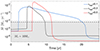 |
Fig. 4. Accretion rate on the star of mass M* = 10 M⊙ during a single TI burst in the models with three different values of αhot–0.1 (blue line), 0.3 (black line), and 0.5 (red line). The horizontal dashed line shows the Ṁth value calculated with Eq. (8). The accretion rate variability below the dashed line (the shaded region) is not observable. The horizontal dotted line shows the Ṁdep, which is equal to ≈ 6.6 × 10⁻⁵ M⊙ yr−1 for all the models. The time instance t = 0 is arbitrary. |
5. Comparison with the observations
To date, only a few observed HMYSO accretion bursts have been characterised sufficiently for a meaningful comparison to our simulations; we list them in Table 3. Their durations range from a few months to at least a decade (Caratti o Garatti et al. 2017; Hunter et al. 2017; Brogan et al. 2019; Proven-Adzri et al. 2019; Stecklum et al. 2021; Chen et al. 2021; Wolf et al. 2024). Here we focus mainly on two properties of the bursts: the peak mass accretion rate during the burst, Ṁpeak, and the duration of the burst. All the observed bursts on HMYSOs have Ṁpeak ≳ 10−3 M⊙ yr−1. The observed short burst durations indicate that the processes leading to the bursts occur in the immediate vicinity of the central star (Elbakyan et al. 2021).
Main properties of outbursting HMYSOs.
The star in M17 NIR is an intermediate-mass star, M* ≈ 5 M⊙. The top panel in Fig. 3 shows that classic TI bursts on these stars are observable for all parameter values considered, due to the relatively low value of threshold Ṁth. The TI bursts in the models with Ṁdep= 3 × 10⁻⁵ M⊙ yr−1 and Ṁdep= 3 × 10⁻⁴ M⊙ yr−1 are not consistent with the those observed in M17 NIR, having either shorter (longer) durations or higher (lower) Ṁpeak values. On the other hand, the TI burst in the model with Ṁdep= 10−4 M⊙ yr−1 has burst duration and Ṁpeak that are consistent with the observed burst in M17 NIR. Thus, TI may be responsible for an outburst on M17 MIR (HMYSO with mass M ≈ 5 M⊙), if the burst had a duration of about a decade and is a singular outburst. However, as was stated earlier, M17 MIR showed multiple outbursts; we address this problem in Sect. 6.
Similar to the models with M* = 5 M⊙, all model TI outbursts on HMYSOs with mass M* = 10 M⊙ are observable (see the middle panel in Fig. 3). However, these outbursts have durations of ≳7 yr, which is longer than the observed outbursts on the HMYSOs of similar mass (0.75−5 yr). Although the estimated mass of NGC 6334I MM1 is about 6.7 M⊙ (Hunter et al. 2021), the burst duration in this HMYSO has a duration of more than 8 yr, resembling the model outburst duration for a M* = 5 M⊙ star.
We arrive at a similar conclusion for TI bursts on HMYSOs with mass M* = 20 M⊙ (see bottom panel in Fig. 3). The TI outbursts in this case are too long compared with the observed short outbursts (< 5 yr), but may be relevant for longer duration ones.
In conclusion, regardless of the value of αhot, Ṁdep, and M* used in the models, TI outbursts may only be responsible for long outbursts (≳5 yr) on HMYSOs. It is also important to note that some HMYSOs have been observed to have multiple outbursts. All the model TI outbursts studied so far were discussed as a singular event, not connected with preceding or subsequent TI outbursts. In the next section we discuss TI as a possible mechanism for triggering multiple outbursts.
6. Multiplicity of the observed bursts
The longest of the bursts observed on a HMYSO to date (M17 MIR, Chen et al. 2021) has a duration of > 10 yr and is still ongoing. Its duration and energy are both a few times longer and higher than those of the other outbursts observed in HMYSOs. The timescales of this outburst are comparable to the FU Ori phenomenon in low-mass protostars. Furthermore, unusually for the outbursts observed on HMYSOs so far, M17 MIR has two accretion outbursts with duration of ∼9 − 20 yr each, separated by a 6 yr quiescent phase. Thus, during the 28 years of the available observations for this source, it spent most of the time in the outburst state (about ∼80%) (Chen et al. 2021). Multiple outbursts may not be unique to M17 MIR. Based on 30 years of sparse K-band photometry, a recent study by Fedriani et al. (2023) suggests that S255IR NIRS3 might have had another outburst, previously unreported, in the late 1980s, many decades before the well-known accretion outburst that was observed in 2015. This may indicate that accretion outbursts in a significant fraction of HMYSOs may have short repetition times (of the order of decades).
In principle, molecular outflows triggered during the accretion outbursts might be observed as distinct outflow knots along the outflow axis. The spacing between knots can be used to determine the time interval between each individual accretion burst, assuming that each knot is associated with an accretion burst (e.g. Vorobyov et al. 2018). It was recently shown by Zhou et al. (2024) that four blue-shifted CO knots along the outflow axis from M17 MIR indicate four clustered accretion outbursts occurring over the past few hundred years, each lasting for tens of years, with the intervals between these clustered accretion outbursts also being approximately tens of years.
6.1. Thermal instability bursts with higher frequency
Thermal instability bursts in all of our models explored earlier in the paper have periodicities of more than a few hundred years, much too long to account for the multiple bursts in M17 MIR and S255IR NIRS3. However, the repetition timescale for classical TI bursts scales with αcold as  (see Sect. 3.4 in Nayakshin et al. 2024). Therefore, here we explore whether higher values of cold disc viscosity could help the TI scenario to produce rapidly repeating bursts.
In the top panel of Fig. 5 we show the TI accretion bursts in HMYSO with 5 M⊙ in two models with different αcold, but with the same αhot = 0.1. We chose the value αcold = 0.05 for one of the models since this value is higher than the conventional value of αcold = 0.01 − 0.02, but still lies close to the values of αcold obtained from the 3D MHD simulations (Coleman et al. 2016; Hirose et al. 2014). Clearly, the model with higher αcold has more frequent TI bursts compared to the model with the classical αcold = 0.01 value. The periodicity of TI bursts in the higher αcold model is 17 years. This is much shorter than the periodicity of TI bursts in αcold = 0.01 model (225 yr), but still longer than the duration of the quiescent period between the outbursts on M17 MIR (6 yr). The higher αcold also impacts the peak accretion rate during the outburst, making it lower (Dubus et al. 2001). The peak mass accretion rates during the TI bursts in the αcold = 0.05 model is 10−3 M⊙ yr−1. Thus, even the higher αcold value shortens the quiescent period between the TI outbursts; it also makes the bursts weaker and still not consistent with the observed counterparts. In the inset we show a zoomed-in image of one of the TI bursts in the higher αcold model. The bursts in the model have durations of a few years, but the interesting feature is the secondary burst happening during the main TI burst. This secondary burst is discussed later in Sect. 6.2. Interestingly, about a year after the outburst, a relatively weak secondary peak is observed in the S255 light curve, also showing some spectroscopic changes around those epochs (Uchiyama et al. 2020).
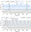 |
Fig. 5. Accretion rate histories for the models with different αcold parameter. In all models, we use αhot = 0.1 and Ṁdep= 10−4 M⊙ yr−1. |
We conducted a similar analysis of αcold impact onto the TI outbursts for our model with 20 M⊙ mass. The results are shown in the bottom panel of Fig. 5. The TI outbursts in the model with higher αcold show behaviour similart to its counterparts on the 5 M⊙ mass HMYSOs discussed earlier. However, due to the higher Ṁacc, only a short period of outburst is observable in the αcold = 0.05 model. The duration of the observable part of the burst is about 2 yr, being consistent with the observed duration on S255IR NIRS3 (2−2.5 yr), but not with that on G323.46−0.08 (8.4 yr). Moreover, the amplitude of the observable part of the model burst changes only by a factor of ≈1.5 in contrast to the observed change in HMYSOs by more than a factor of 5 or even an order of magnitude. The quiescent period between the TI bursts in αcold = 0.05 is about 50 years, which is about two times longer than the period of 25 − 30 years between the possible bursts in S255 NIRS3. Thus, the models with higher αcold are not able to reproduce the multiple outbursts on HMYSOs with the observed properties. The burst properties in the models with various αcold are summarised in Table 4.
In the next section we discuss the reflare mechanism responsible for the secondary outbursts in the model αcold = 0.05 with 5 M⊙ mass. We investigate the possibility of explaining the observed outburst multiplicity with the secondary outbursts.
6.2. Reflares
The occurrence of multiple secondary outbursts called reflares during the outburst decay is a well-known feature of TI models of discs (Menou et al. 2000; Dubus et al. 2001). Reflares arise when the surface density behind the cooling front of the initial TI outburst achieves the critical density at which the disc enters a state of thermal instability, initiating the development of a new heating front. This front expands outward in an inside-out manner, reheating the disc until the surface density falls below the critical value, allowing cooling to recommence. However, reflares do not typically occur in dwarf novae or low-mass X-ray binary transients (Coleman et al. 2016); they do appear in accretion discs around a neutron star, but at very small radii (Dubus et al. 2001). Furthermore, recently Nayakshin et al. (2024) has argued that reflares may have been observed in several ‘unusual’ (i.e. lasting only a few years rather than centuries) FUor outbursts on stars with mass M* ≲ 1 M⊙. It is therefore interesting to consider whether reflares are present in models of TI in discs around high-mass stars, and whether they are observable.
The emergence of reflares and their characteristics depend on multiple factors, for example disc viscosity, the size of the unstable region, disc irradiation by the central object, magnetic torques, and the shape of the S-curve (Nayakshin et al. 2024). For high-mass stars, magnetospheric torques on the disc are likely to be negligible because only 7 ± 3% of high-mass stars show large-scale surface magnetic fields (Grunhut et al. 2017).
We started by varying the Tcrit parameter in our models. As shown in Nayakshin et al. (2024), the unstable branch of the S-curve shifts closer to the hot stable branch as Tcrit increases, supporting the presence of reflares after the initial TI burst’s decline. In the top panel of Fig. 6 we show the short period of accretion rate histories for three different models, during which a TI outburst is present. All three models have a stellar mass of 5 M⊙ and Ṁdep = 10−4 M⊙ yr−1; however, they differ by the value of Tcrit. Clearly, the higher Tcrit models show reflares. In the model with Tcrit = 15 000 K (black line), only one reflare is triggered, which takes place about 25 years later than the initial TI burst. This quiescent time period between the bursts is much longer than that for M17 MIR (6 yr). The durations of the initial burst and the reflare in this model are ≈9 and 4 yr, respectively. The duration of the reflare is shorter by a factor of 2 at least than the duration observed for M17 MIR (≳9 yr). In order to decrease the quiescent period between the bursts, we recalculated the model, increasing Tcrit to 25 000 K (red line). Clearly, multiple reflares are present in this model with the quiescent period between the bursts varying from 3 to 22 years, which are in the range of the observed values. However, the durations of the bursts are only 2 − 3 yr (a factor of a few shorter than the observed bursts) and the peak accretion rates during the bursts are ≈ 6 × 10⁻⁴ M⊙ yr−1 (a factor of few lower than the observed bursts). This means that the reflares are unlikely to be responsible for the multiple outbursts on HMYSOs with 5 M⊙ mass, for example M17 MIR.
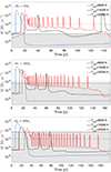 |
Fig. 6. Accretion rate histories for the models with different stellar masses and with three different values of Tcrit: 8000 K (blue line), 15 000 K (black line), and 25 000 K (red line) for each stellar mass. In all models, we use αhot = 0.1 and Ṁdep = 10−4 M⊙ yr−1. |
We carried out a similar study for the 20 M⊙ mass HMYSO, and the results are shown in the bottom panel of Fig. 6. Similar to the 5 M⊙ mass models shown earlier, the reflares emerge once the value of Tcrit in the model increases. However, due to the high Ṁacc, the reflares are not observable and only the initial TI outburst is observable. Thus, the reflares are most probably not responsible for the multiple outbursts on HMYSOs with 20 M⊙ mass.
Multiple bursts have not yet been observed on HMYSOs with masses of 10 M⊙; however, we calculated similar models with 10 M⊙ and show the results in the middle panel of Fig. 6. These results could possibly serve as a prediction for future outburst observation on the 10 M⊙ HMYSOs. In the model with Tcrit = 15 000 K (black line), two reflares are triggered after the initial TI burst. The reflares are separated by a quiescent time period of 18 yr and have durations of about 3 yr. The peak accretion rate for the first reflare is Ṁpeak ≈ 10−3 M⊙ yr−1, which is close to the observed values, while the second reflare has Ṁpeak ≈ 7 × 10⁻⁴ M⊙ yr−1. Thus, the first reflare has properties close to that of the observed bursts in one of the HMYSOs with a stellar mass of 10 M⊙, V723 Car. However, the burst observed in other HMYSO with a stellar mass of 10 M⊙, G358.93−0.03 MM1, has a duration of a few months, which could not be reproduced with TI outbursts or the reflares in this model. In order to make the duration of the reflares shorter and try to fit the observations, we calculated another model with Tcrit = 25 000 K (red line). As in the case of the 5 M⊙ and 20 M⊙ models, multiple reflares were triggered that have durations of about 1 yr, and the quiescent periods between the reflares increased with time from ≈1.5 yr to about ≈15 yr. However, the peak accretion rate values of the reflares were much lower than observed, being in average about Ṁpeak ≈ 4 × 10⁻⁴ M⊙ yr−1. This again led to the conclusion, that the observed short (< 1 yr) outbursts are unlikely to be caused by the TI or the reflares. Although, some observed outbursts could be a result not of the initial TI outbursts (which we overlook in this paper), but of the subsequent reflare. The burst properties of the models with various Tcrit are summarised in Table 5.
7. Discussion
7.1. Comparison with the photometric data of S255IR NIRS3
One of the important features in the S255 NIRS3 burst is the increase in luminosity in K band (λ = 2.2 μm) by > 2 mag (Caratti o Garatti et al. 2017). In order to compare our model results with the observational data, we generated integrated black-body spectra of the disc using our time-dependent models, and determined the observed magnitudes of the disc within our computational domain, excluding the star and the envelope. For the source distance, we assumed 1.78 kpc (Burns et al. 2016) and for the optical extinction (AV) a value of 44 mag (Caratti o Garatti et al. 2017).
In the top panel of Fig. 7, we show the mass accretion rate during one of the TI outbursts on HMYSO with the mass of 20 M⊙. The horizontal dashed line shows the Ṁth value. The black solid line in the second panel shows the model magnitude in the photometric K band (λ = 2.2 μm) during the TI outburst. The blue dots in the second panel show the K-band photometry data for S255IR NIRS3 source obtained from Fedriani et al. (2023). The time instance t = 0 corresponds to the beginning of model TI outburst and the confirmed outburst registered in June 2015 on the S255IR NIRS3 source. Clearly, in the model the increase in K band due to the outburst is ∼1 mag, while the observed K band for S255IR NIRS3 increased by a few magnitudes during the outburst. Meanwhile, the increase in the mass accretion rate during the model TI outburst is consistent with the change in mass accretion rate for S255IR NIRS3 during the outburst, estimated from the observations. Thus, even if the model peak accretion rates during the burst and the burst duration are similar to the observed values, a strong inconsistency can still be present between the model and the observational luminosities in some photometric bands.
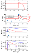 |
Fig. 7. Comparison of mass accretion rates, K-Band magnitudes, and observations during a TI outburst. Top panel: Mass accretion rate onto the star of mass M* = 20 M⊙ during a TI outburst. The horizontal dashed line shows the Ṁth value calculated with Eq. (8). Second panel: Model K-band magnitudes during the TI outbursts (solid black line) and the observed K-band photometry for the S255IR NIRS3 source from Fedriani et al. (2023) (blue dots). The K-band magnitudes for the model with the optical extinction Av = 60 is shown with the dashed black line. The red line corresponds to the model B-band magnitudes. The time t = 0 corresponds to the beginning of the model TI outburst and to the beginning of the observed outburst on S255IR NIRS3 registered in June 2015. Third panel: K-band magnitudes for the model presented in the top two panels of the figure (black line) and for two other models with the higher Ṁdep. The blue dots represent the observational data also shown in the second panel. Bottom panel: Mass accretion rate histories during the TI bursts in the models shown in the third panel with the corresponding colour. The horizontal dashed line marks the Ṁth value. The time t = 0 is similar to that in the top two panels. The blue dot marks the observed peak mass-accretion rate value on S255IR NIRS3 during the outburst. |
We note that the model pre-burst K-band magnitudes are much higher than the observed values if we use Av = 44 mag. However, the estimated error range for the observed value of Av is quite large, being ±16 mag (Caratti o Garatti et al. 2017). If we use the highest value in this error range, Av = 60 mag, then the pre-burst K-band magnitudes in our model fits the observations very well. The K-band magnitudes for the model with higher Av are shown with the dashed line in the second panel of Fig. 7. The increase in the K band during the outburst is again only about one magnitude, which is much lower than the observed value. This result emphasises the importance of not only comparing model mass accretion rates during the bursts and their durations, but also of conducting photometric analysis to comprehensively assess the agreement between model predictions and observational data.
Some of the observed variability (a few magnitudes) in K band may also be due to the variability of AV during the burst. Extinction variation (pre- or post-burst) is observed for some FUors (Guo et al. 2024), and is often attributed to dust grain condensation when the wind collides with the envelope (Siwak et al. 2023) or to dust ejection during the bursts. This observed change in extinction occurs on short timescales of years.
The reason for the low variability in the model K band is that the effective temperatures corresponding to this wavelength (∼1300 K) are present in the disc at the radial distance of ∼1 − 2 AU. At this radius, the influence of the TI outburst is much weaker, compared to the sub-AU distances in the disc. For comparison, we present in the second panel of Fig. 7 the model B-band magnitudes (red line), which correspond to the inner and hotter regions of the disc (∼6600 K). Clearly, the increase in B band is stronger, reaching about 2 mag.
In order to show which TI bursts will ensure the change in the K band for more than two magnitudes in a HMYSO of 20 M⊙, we varied the value of Ṁdep in our model, while fixing the rest of the model parameters. The results for these models are shown in the bottom two panels of Fig. 7. The black line in the bottom two panels corresponds to the model with Ṁdep = 3 × 10⁻⁵ M⊙ yr−1 shown in the top two panels. The two other models with Ṁdep = 3 × 10⁻⁴ M⊙ yr−1 and Ṁdep = 3 × 10⁻³ M⊙ yr−1 are presented in the bottom two panels of the figure with red and blue lines, respectively. Clearly, to have an increase of > 2 mag in K band during a TI outburst, one should have Ṁdep > a few × 10−4 M⊙ yr−1. The latter values are in agreement with the observed values for the outbursting HMYSOs (Beuther et al. 2013; Moscadelli et al. 2021). However, as can be seen in the bottom panel of Fig. 7, the peak accretion rates during such a TI outburst will have values Ṁpeak ≳ 10−2 M⊙ yr−1, which is much higher than the observed values of peak accretion rates in S255IR NIRS3 source during its outburst event (blue dot). Moreover, the burst duration in the models with higher Ṁdep increases to a few tens of years (red line) and to more than one hundred years (blue line), which are much longer than the observed duration of the bursts in S255IR NIRS3. Another burst feature that becomes strongly inconsistent with the observations for the higher Ṁdep models is the rise time of the burst. The rise time also increases and becomes a few years (red line) and more than a decade (blue line), which are much longer than the observed value of 0.4 yr for S255IR NIRS3. Thus, the observed strong variability (> 2 mag) in K band during a short period of time (∼2 yr) in the S255IR NIRS3 source most likely is not a result of TI burst in the inner disc.
7.2. Possible mechanisms responsible for bursts on HMYSOs
Our analysis of TI models in the context of HMYSO outbursts reveals their potential to explain some key characteristics, such as burst duration and magnitude. However, several critical discrepancies emerge when comparing the model predictions with the observed phenomena.
One notable limitation of current TI models is their inability to fully account for the multiplicity of bursts observed in some HMYSOs. While the simulations accurately reproduce individual outbursts in terms of duration and magnitude in some systems, they fail to capture the sequential or recurrent nature of burst occurrences observed in other systems. This discrepancy suggests that additional factors or mechanisms may be at play in regulating the burst frequency and timing in HMYSOs.
One possible avenue for addressing this inconsistency is the consideration of external influences, such as gravitational interactions or disc instabilities. In addition to TI, gravitational instability (GI) and disc fragmentation have been proposed as alternative mechanisms for triggering the observed outbursts in HMYSOs (Meyer et al. 2017; Oliva & Kuiper 2020; Elbakyan et al. 2021, 2023). In this scenario, the disc undergoes fragmentation into clumps, which can then accrete onto the central protostar, triggering episodic bursts of accretion and mass ejection. While thermal instability remains a candidate for explaining HMYSO outbursts, the roles of gravitational instability and disc fragmentation warrant further investigation. Future studies incorporating these mechanisms into comprehensive numerical simulations could provide valuable insights into the relative contributions of each process to the observed burst phenomena. By exploring a diverse range of physical conditions and initial parameters, we can assess the viability of gravitational instability and disc fragmentation as complementary or alternative mechanisms for driving episodic accretion in HMYSOs.
Furthermore, the observed diversity in burst characteristics among different HMYSOs underscores the need for a more nuanced approach to model these phenomena. Future efforts should aim to develop more sophisticated TI models that can account for the full range of observed behaviours, including both singular and multiple burst events. Incorporating observational constraints from a broader sample of HMYSOs will be crucial for refining and validating these models, ultimately advancing our understanding of the underlying processes driving star formation and evolution.
7.3. Parameter space study
Additionally, it is important to note that our TI models contain several free parameters that are adjusted to match observed burst characteristics. While we have explored a range of parameter values by varying them, it is impractical to comprehensively study all possible combinations of parameters due to the vastness of the parameter space. However, it is worth highlighting that the diverse combinations of free parameters in the models can yield new and interesting results, potentially revealing novel insights into HMYSO outburst phenomena.
The exploration of different parameter sets may uncover previously unexplored regimes of behaviour, shedding light on the underlying physical processes driving burst initiation and evolution. While our current study focuses on a subset of parameter values that produce reasonable agreement with some observed burst characteristics, a comprehensive exploration of the parameter space remains a valuable avenue for future research. Such an endeavour would involve systematic investigations of a broader range of parameter values, potentially uncovering new regimes of behaviour and refining our understanding of HMYSO outburst mechanisms. By leaving this comprehensive parameter space study for future work, we open the door to further advancements in our modelling efforts and a deeper understanding of the complex interplay between physical processes governing HMYSO evolution.
7.4. 1D versus multi-D models
We acknowledge the limitations of our 1D modelling of HMYSO accretion discs. While 1D models provide valuable insights into the basic physical processes governing disc evolution and outburst phenomena, they inherently oversimplify the complex interplay of dynamics occurring within the disc. The transition to 2D or 3D modelling represents a crucial step towards capturing the intricate dynamics of HMYSO accretion discs, allowing a more realistic treatment of phenomena such as disc fragmentation, gravitational instabilities, and the formation of protostellar companions. By incorporating azimuthal variations in disc structure and evolution, multi-dimensional models offer a more accurate representation of the processes driving episodic accretion in HMYSOs. Future studies employing multi-dimensional hydrodynamic simulations are essential for elucidating the role of disc morphology, turbulence, and non-axisymmetric structures in shaping the observed burst behaviour of HMYSOs. The first steps in this direction have already been taken by Jordan et al. (2024) with the new FargoCPT code (Rometsch et al. 2024). The authors simulate complete outburst cycles using the thermal tidal instability model in non-isothermal, viscous accretion discs in cataclysmic variable systems.
8. Conclusions
In this paper, using the 1D hydrodynamical code DEO, we studied the phenomenon of thermal instability (TI) outbursts on high-mass young stellar objects (HMYSOs) and their implications for the early stages of massive star formation. This modelling allowed us to quantify TI outburst properties and their dependence on model parameters, such as stellar mass and the viscosity prescription. Our main conclusions are the following:
-
Our simulations reproduce the main characteristics of the longer bursts observed in HMYSOs reasonably well. However, they fail to reproduce the short-duration outbursts (less than a few years) with the short rise times (a few weeks or months) observed in several HMYSOs. This suggests another mechanism, such as disc fragmentation, as a potential alternative in generating these shorter outbursts (cf. Sect. 7.2).
-
Although our TI models explore a wide parameter space in αhot, Ṁdep, and M*, they struggle to reproduce multiple outbursts observed in a few sources (Sects. 5 and 6). Notably, the recurrent outbursts in observed systems, such as M17 MIR and possibly S255 NIRS3, characterised by sequential bursts separated by relatively short quiescent phases, pose a challenge to the current TI models. More specifically, the repetition timescale of model outbursts is too long for the repetitions to be humanly observed (cf. Table 1). This discrepancy signals the need for a refined or alternative mechanism to comprehensively elucidate the observed multiplicity and frequency of bursts in HMYSOs.
-
SED modelling of TI outbursts (Sect. 7.1) shows that TI outburst model luminosity in various photometric bands can strongly differ from the observed values, even though the model displays a Ṁ∗ value similar to that inferred observationally. This indicates that the model flux as a function of radius in the disc is different from that of the system modelled, and is therefore an important tool that modellers should not neglect to use.
-
While our model TI outbursts do not offer a comprehensive explanation for the whole range of the observed episodic accretion variability in HMYSOs, they do show TI to be an important part of the disc physics of these objects. TI sculpts the structure of the inner few AU of HMYSO discs and cannot be simply discounted as ‘unwanted because not quite successful’. Any other accretion variability agent, such as massive migrating clumps, must contend with the effects that TI has on the inner disc. This should not be viewed as a modelling nuisance, but be instead embraced as an additional tool to probe potential scenarios for HMYSO accretion outbursts.
Our study demonstrates that TI accretion outbursts are a common occurrence in high-mass YSOs, during their early stages of formation. These bursts of accretion provide important insights into the mass accretion process, the evolution of circumstellar discs, and the formation of multiple star systems. Further investigations combining observational studies with theoretical modelling will contribute to a more comprehensive understanding of the complex processes involved in the birth of massive stars.
Acknowledgments
We thank the anonymous referee for their thoughtful and insightful feedback, which has greatly improved the quality of this paper. V.E. and S.N. acknowledge the funding from the UK Science and Technologies Facilities Council, grant No. ST/S000453/1. This work made use of the DiRAC Data Intensive service at Leicester, operated by the University of Leicester IT Services, which forms part of the STFC DiRAC HPC Facility (www.dirac.ac.uk). C.G. acknowledges support from PRIN-MUR 2022 20228JPA3A “The path to star and planet formation in the JWST era (PATH)” funded by NextGeneration EU and by INAF-GoG 2022 “NIR-dark Accretion Outbursts in Massive Young stellar objects (NAOMY)” and Large Grant INAF 2022 “YSOs Outflows, Disks and Accretion: towards a global framework for the evolution of planet forming systems (YODA)”. R.K. acknowledges financial support via the Heisenberg Research Grant funded by the Deutsche Forschungsgemeinschaft (DFG, German Research Foundation) under grant no. KU 2849/9, project no. 445783058.
References
- Ahmadi, A., Beuther, H., Bosco, F., et al. 2023, A&A, 677, A171 [NASA ADS] [CrossRef] [EDP Sciences] [Google Scholar]
- Armitage, P. J. 2015, ArXiv e-prints [arXiv:1509.06382] [Google Scholar]
- Armitage, P. J., Livio, M., & Pringle, J. E. 2001, MNRAS, 324, 705 [NASA ADS] [CrossRef] [Google Scholar]
- Audard, M., Ábrahám, P., Dunham, M. M., et al. 2014, Protostars and Planets VI (Tucson: University of Arizona Press) [Google Scholar]
- Bai, X.-N., & Stone, J. M. 2013, ApJ, 769, 76 [Google Scholar]
- Beckwith, K., Armitage, P. J., & Simon, J. B. 2011, MNRAS, 416, 361 [NASA ADS] [Google Scholar]
- Bell, K. R., & Lin, D. N. C. 1994, ApJ, 427, 987 [NASA ADS] [CrossRef] [Google Scholar]
- Beltrán, M. T., & de Wit, W. J. 2016, A&ARv, 24, 6 [Google Scholar]
- Beuther, H., Linz, H., & Henning, T. 2013, A&A, 558, A81 [NASA ADS] [CrossRef] [EDP Sciences] [Google Scholar]
- Beuther, H., Walsh, A. J., Johnston, K. G., et al. 2017, A&A, 603, A10 [NASA ADS] [CrossRef] [EDP Sciences] [Google Scholar]
- Borchert, E. M. A., Price, D. J., Pinte, C., & Cuello, N. 2022, MNRAS, 517, 4436 [CrossRef] [Google Scholar]
- Brogan, C. L., Hunter, T. R., Towner, A. P. M., et al. 2019, ApJ, 881, L39 [NASA ADS] [CrossRef] [Google Scholar]
- Burns, R. A., Handa, T., Nagayama, T., Sunada, K., & Omodaka, T. 2016, MNRAS, 460, 283 [NASA ADS] [CrossRef] [Google Scholar]
- Cannizzo, J. K. 1993, ApJ, 419, 318 [NASA ADS] [CrossRef] [Google Scholar]
- Caratti o Garatti, A., Stecklum, B., Garcia Lopez, R., et al. 2017, Nat. Phys., 13, 276 [Google Scholar]
- Cesaroni, R., Galli, D., Lodato, G., Walmsley, M., & Zhang, Q. 2006, Nature, 444, 703 [NASA ADS] [CrossRef] [Google Scholar]
- Chen, Z., Sun, W., Chini, R., et al. 2021, ApJ, 922, 90 [NASA ADS] [CrossRef] [Google Scholar]
- Coleman, M. S. B., Kotko, I., Blaes, O., Lasota, J. P., & Hirose, S. 2016, MNRAS, 462, 3710 [NASA ADS] [CrossRef] [Google Scholar]
- Coleman, M. S. B., Blaes, O., Hirose, S., & Hauschildt, P. H. 2018, ApJ, 857, 52 [NASA ADS] [CrossRef] [Google Scholar]
- Commerçon, B., González, M., Mignon-Risse, R., Hennebelle, P., & Vaytet, N. 2022, A&A, 658, A52 [NASA ADS] [CrossRef] [EDP Sciences] [Google Scholar]
- Contreras Peña, C., Lucas, P. W., Guo, Z., & Smith, L. 2024, MNRAS, 528, 1823 [Google Scholar]
- Cuello, N., Ménard, F., & Price, D. J. 2023, Eur. Phys. J. Plus, 138, 11 [NASA ADS] [CrossRef] [Google Scholar]
- Davis, S. W., Stone, J. M., & Pessah, M. E. 2010, ApJ, 713, 52 [NASA ADS] [CrossRef] [Google Scholar]
- Dubus, G., Hameury, J. M., & Lasota, J. P. 2001, A&A, 373, 251 [NASA ADS] [CrossRef] [EDP Sciences] [Google Scholar]
- Elbakyan, V. G., Nayakshin, S., Vorobyov, E. I., Caratti o Garatti, A., & Eislöffel, J. 2021, A&A, 651, L3 [NASA ADS] [CrossRef] [EDP Sciences] [Google Scholar]
- Elbakyan, V. G., Nayakshin, S., Meyer, D. M. A., & Vorobyov, E. I. 2023, MNRAS, 518, 791 [Google Scholar]
- Fedriani, R., Caratti o Garatti, A., Cesaroni, R., et al. 2023, A&A, 676, A107 [NASA ADS] [CrossRef] [EDP Sciences] [Google Scholar]
- Fischer, W. J., Hillenbrand, L. A., Herczeg, G. J., et al. 2023, ASP Conf. Ser., 534, 355 [NASA ADS] [Google Scholar]
- Flock, M., Dzyurkevich, N., Klahr, H., Turner, N. J., & Henning, T. 2011, ApJ, 735, 122 [NASA ADS] [CrossRef] [Google Scholar]
- Fromang, S., & Nelson, R. P. 2006, A&A, 457, 343 [NASA ADS] [CrossRef] [EDP Sciences] [Google Scholar]
- Grunhut, J. H., Wade, G. A., Neiner, C., et al. 2017, MNRAS, 465, 2432 [NASA ADS] [CrossRef] [Google Scholar]
- Guo, Z., Lucas, P. W., Kurtev, R. G., et al. 2024, MNRAS, 529, L115 [Google Scholar]
- Hameury, J. M. 2020, Adv. Space Res., 66, 1004 [Google Scholar]
- Hameury, J.-M., Menou, K., Dubus, G., Lasota, J.-P., & Hure, J.-M. 1998, MNRAS, 298, 1048 [Google Scholar]
- Hartmann, L., & Kenyon, S. J. 1996, ARA&A, 34, 207 [NASA ADS] [CrossRef] [Google Scholar]
- Herbig, G. H. 1977, ApJ, 217, 693 [NASA ADS] [CrossRef] [Google Scholar]
- Herbig, G. H. 1989, Eur. South. Obs. Conf. Workshop Proc., 33, 233 [NASA ADS] [Google Scholar]
- Hirose, S. 2015, MNRAS, 448, 3105 [NASA ADS] [CrossRef] [Google Scholar]
- Hirose, S., Krolik, J. H., & Stone, J. M. 2006, ApJ, 640, 901 [NASA ADS] [CrossRef] [Google Scholar]
- Hirose, S., Blaes, O., Krolik, J. H., Coleman, M. S. B., & Sano, T. 2014, ApJ, 787, 1 [NASA ADS] [CrossRef] [Google Scholar]
- Hōshi, R. 1979, Progr. Theor. Phys., 61, 1307 [Google Scholar]
- Hosokawa, T., & Omukai, K. 2009, ApJ, 691, 823 [Google Scholar]
- Hosokawa, T., Hirano, S., Kuiper, R., et al. 2016, ApJ, 824, 119 [NASA ADS] [CrossRef] [Google Scholar]
- Hunter, T. R., Brogan, C. L., MacLeod, G., et al. 2017, ApJ, 837, L29 [NASA ADS] [CrossRef] [Google Scholar]
- Hunter, T. R., Brogan, C. L., MacLeod, G. C., et al. 2018, ApJ, 854, 170 [NASA ADS] [CrossRef] [Google Scholar]
- Hunter, T. R., Brogan, C. L., De Buizer, J. M., et al. 2021, ApJ, 912, L17 [CrossRef] [Google Scholar]
- Jordan, L. M., Wehner, D., & Kuiper, R. 2024, A&A, 689, A354 [NASA ADS] [CrossRef] [EDP Sciences] [Google Scholar]
- Kadam, K., Vorobyov, E., Regály, Z., Kóspál, Á., & Ábrahám, P. 2020, ApJ, 895, 41 [NASA ADS] [CrossRef] [Google Scholar]
- King, A. R., Pringle, J. E., & Livio, M. 2007, MNRAS, 376, 1740 [NASA ADS] [CrossRef] [Google Scholar]
- Kley, W., & Lin, D. N. C. 1996, ApJ, 461, 933 [Google Scholar]
- Krumholz, M. R., McKee, C. F., & Klein, R. I. 2004, ApJ, 611, 399 [NASA ADS] [CrossRef] [Google Scholar]
- Kuffmeier, M., Frimann, S., Jensen, S. S., & Haugbølle, T. 2018, MNRAS, 475, 2642 [NASA ADS] [CrossRef] [Google Scholar]
- Kuiper, R., & Yorke, H. W. 2013, ApJ, 772, 61 [Google Scholar]
- Lasota, J.-P. 2001, New Astron. Rev., 45, 449 [Google Scholar]
- Lin, D. N. C., Papaloizou, J., & Faulkner, J. 1985, MNRAS, 212, 105 [NASA ADS] [CrossRef] [Google Scholar]
- Lodato, G., & Clarke, C. J. 2004, MNRAS, 353, 841 [NASA ADS] [CrossRef] [Google Scholar]
- Machida, M. N., Inutsuka, S.-I., & Matsumoto, T. 2011, ApJ, 729, 42 [NASA ADS] [CrossRef] [Google Scholar]
- Mendigutía, I. 2020, Galaxies, 8, 39 [Google Scholar]
- Menou, K., Hameury, J.-M., & Stehle, R. 1999, MNRAS, 305, 79 [Google Scholar]
- Menou, K., Hameury, J.-M., Lasota, J.-P., & Narayan, R. 2000, MNRAS, 314, 498 [Google Scholar]
- Meyer, F., & Meyer-Hofmeister, E. 1981, A&A, 104, L10 [NASA ADS] [Google Scholar]
- Meyer, D. M.-A., Vorobyov, E. I., Kuiper, R., & Kley, W. 2017, MNRAS, 464, L90 [NASA ADS] [CrossRef] [Google Scholar]
- Meyer, D. M. A., Kreplin, A., Kraus, S., et al. 2019, MNRAS, 487, 4473 [NASA ADS] [CrossRef] [Google Scholar]
- Mignon-Risse, R., González, M., Commerçon, B., & Rosdahl, J. 2020, A&A, 635, A42 [NASA ADS] [CrossRef] [EDP Sciences] [Google Scholar]
- Miller, K. A., & Stone, J. M. 2000, ApJ, 534, 398 [NASA ADS] [CrossRef] [Google Scholar]
- Moscadelli, L., Beuther, H., Ahmadi, A., et al. 2021, A&A, 647, A114 [EDP Sciences] [Google Scholar]
- Nayakshin, S., & Elbakyan, V. 2024, MNRAS, 528, 2182 [Google Scholar]
- Nayakshin, S., & Lodato, G. 2012, MNRAS, 426, 70 [Google Scholar]
- Nayakshin, S., Elbakyan, V., & Rosotti, G. 2022, MNRAS, 512, 6038 [NASA ADS] [CrossRef] [Google Scholar]
- Nayakshin, S., Owen, J. E., & Elbakyan, V. 2023, MNRAS, 523, 385 [Google Scholar]
- Nayakshin, S., Cruz Sáenz de Miera, F., Kóspál, Á., et al. 2024, MNRAS, 530, 1749 [NASA ADS] [CrossRef] [Google Scholar]
- Oliva, G. A., & Kuiper, R. 2020, A&A, 644, A41 [NASA ADS] [CrossRef] [EDP Sciences] [Google Scholar]
- Proven-Adzri, E., MacLeod, G. C., Heever, S. P. V. D., et al. 2019, MNRAS, 487, 2407 [Google Scholar]
- Rometsch, T., Jordan, L. M., Moldenhauer, T. W., et al. 2024, A&A, 684, A192 [NASA ADS] [CrossRef] [EDP Sciences] [Google Scholar]
- Sabatini, G., Bovino, S., Giannetti, A., et al. 2021, A&A, 652, A71 [NASA ADS] [CrossRef] [EDP Sciences] [Google Scholar]
- Scepi, N., Lesur, G., Dubus, G., & Flock, M. 2018, A&A, 609, A77 [NASA ADS] [CrossRef] [EDP Sciences] [Google Scholar]
- Shakura, N. I., & Sunyaev, R. A. 1973, A&A, 24, 337 [NASA ADS] [Google Scholar]
- Shi, J., Krolik, J. H., & Hirose, S. 2010, ApJ, 708, 1716 [NASA ADS] [CrossRef] [Google Scholar]
- Simon, J. B., Beckwith, K., & Armitage, P. J. 2012, MNRAS, 422, 2685 [NASA ADS] [CrossRef] [Google Scholar]
- Siwak, M., Hillenbrand, L. A., Kóspál, Á., et al. 2023, MNRAS, 524, 5548 [NASA ADS] [CrossRef] [Google Scholar]
- Smak, J. 1999, Acta Astron., 49, 391 [NASA ADS] [Google Scholar]
- Stecklum, B., Wolf, V., Linz, H., et al. 2021, A&A, 646, A161 [EDP Sciences] [Google Scholar]
- Tanaka, K. E. I., Tan, J. C., & Zhang, Y. 2017, ApJ, 835, 32 [NASA ADS] [CrossRef] [Google Scholar]
- Tapia, M., Roth, M., & Persi, P. 2015, MNRAS, 446, 4088 [Google Scholar]
- Uchiyama, M., Yamashita, T., Sugiyama, K., et al. 2020, PASJ, 72, 4 [NASA ADS] [CrossRef] [Google Scholar]
- Vorobyov, E. I., & Basu, S. 2010, ApJ, 719, 1896 [NASA ADS] [CrossRef] [Google Scholar]
- Vorobyov, E. I., & Elbakyan, V. G. 2018, A&A, 618, A7 [NASA ADS] [CrossRef] [EDP Sciences] [Google Scholar]
- Vorobyov, E. I., Elbakyan, V. G., Plunkett, A. L., et al. 2018, A&A, 613, A18 [NASA ADS] [CrossRef] [EDP Sciences] [Google Scholar]
- Vorobyov, E. I., Khaibrakhmanov, S., Basu, S., & Audard, M. 2020, A&A, 644, A74 [NASA ADS] [CrossRef] [EDP Sciences] [Google Scholar]
- Wolf, V., Stecklum, B., Caratti o Garatti, A., et al. 2024, A&A, 688, A8 [NASA ADS] [CrossRef] [EDP Sciences] [Google Scholar]
- Zapata, L. A., Ho, P. T. P., Schilke, P., et al. 2009, ApJ, 698, 1422 [NASA ADS] [CrossRef] [Google Scholar]
- Zhang, Y.-K., Chen, X., Sobolev, A. M., et al. 2022, ApJS, 260, 34 [NASA ADS] [CrossRef] [Google Scholar]
- Zhao, B., Caselli, P., Li, Z.-Y., & Krasnopolsky, R. 2018, MNRAS, 473, 4868 [Google Scholar]
- Zhou, W., Chen, Z., Jiang, Z., Feng, H., & Jiang, Y. 2024, ApJ, 969, L6 [NASA ADS] [CrossRef] [Google Scholar]
- Zhu, Z., Hartmann, L., & Gammie, C. 2009, ApJ, 694, 1045 [Google Scholar]
- Zhu, Z., Hartmann, L., & Gammie, C. 2010, ApJ, 713, 1143 [Google Scholar]
All Tables
All Figures
|
Fig. 1. Evolution of disc properties and mass accretion rate during a thermal instability outburst. Top four panels: Radial profiles of gas surface density (top panel), midplane disc temperature (second panel), effective disc temperature (third panel), and disc aspect ratio (fourth panel) for five distinct time instances. Bottom panel: Mass accretion rate history onto the HMYSO during the TI outburst. The vertical dashed lines indicate the time instances for which the radial profiles with corresponding colours are shown in the top panels. The horizontal dashed line shows the value of Ṁth calculated with Eq. (8). The shaded area shows the non-observable part of the accretion rate variations. |
| In the text | |
|
Fig. 2. Accretion rate onto the star of mass M* = 5 M⊙ (top panel), M* = 10 M⊙ (middle panel), and M* = 20 M⊙ (bottom panel) during TI bursts for three different values of Ṁdep–3 × 10⁻⁵ M⊙ yr−1 (blue line), 10−4 M⊙ yr−1 (black line), and 3 × 10⁻⁴ M⊙ yr−1 (red line). The horizontal black dashed line shows the Ṁth value for each stellar mass calculated with Eq. (8). The accretion rate variability below the dashed line (shaded region) is unlikely to be observable. The horizontal dotted lines show the Ṁdep for each model with the corresponding colour. The time instance t = 0 in all panels of the figure is arbitrary. |
| In the text | |
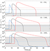 |
Fig. 3. Similar to Fig. 2, but zoomed-in on a single TI outburst in each model. |
| In the text | |
|
Fig. 4. Accretion rate on the star of mass M* = 10 M⊙ during a single TI burst in the models with three different values of αhot–0.1 (blue line), 0.3 (black line), and 0.5 (red line). The horizontal dashed line shows the Ṁth value calculated with Eq. (8). The accretion rate variability below the dashed line (the shaded region) is not observable. The horizontal dotted line shows the Ṁdep, which is equal to ≈ 6.6 × 10⁻⁵ M⊙ yr−1 for all the models. The time instance t = 0 is arbitrary. |
| In the text | |
|
Fig. 5. Accretion rate histories for the models with different αcold parameter. In all models, we use αhot = 0.1 and Ṁdep= 10−4 M⊙ yr−1. |
| In the text | |
|
Fig. 6. Accretion rate histories for the models with different stellar masses and with three different values of Tcrit: 8000 K (blue line), 15 000 K (black line), and 25 000 K (red line) for each stellar mass. In all models, we use αhot = 0.1 and Ṁdep = 10−4 M⊙ yr−1. |
| In the text | |
|
Fig. 7. Comparison of mass accretion rates, K-Band magnitudes, and observations during a TI outburst. Top panel: Mass accretion rate onto the star of mass M* = 20 M⊙ during a TI outburst. The horizontal dashed line shows the Ṁth value calculated with Eq. (8). Second panel: Model K-band magnitudes during the TI outbursts (solid black line) and the observed K-band photometry for the S255IR NIRS3 source from Fedriani et al. (2023) (blue dots). The K-band magnitudes for the model with the optical extinction Av = 60 is shown with the dashed black line. The red line corresponds to the model B-band magnitudes. The time t = 0 corresponds to the beginning of the model TI outburst and to the beginning of the observed outburst on S255IR NIRS3 registered in June 2015. Third panel: K-band magnitudes for the model presented in the top two panels of the figure (black line) and for two other models with the higher Ṁdep. The blue dots represent the observational data also shown in the second panel. Bottom panel: Mass accretion rate histories during the TI bursts in the models shown in the third panel with the corresponding colour. The horizontal dashed line marks the Ṁth value. The time t = 0 is similar to that in the top two panels. The blue dot marks the observed peak mass-accretion rate value on S255IR NIRS3 during the outburst. |
| In the text | |
Current usage metrics show cumulative count of Article Views (full-text article views including HTML views, PDF and ePub downloads, according to the available data) and Abstracts Views on Vision4Press platform.
Data correspond to usage on the plateform after 2015. The current usage metrics is available 48-96 hours after online publication and is updated daily on week days.
Initial download of the metrics may take a while.