| Issue |
A&A
Volume 676, August 2023
|
|
|---|---|---|
| Article Number | A107 | |
| Number of page(s) | 10 | |
| Section | Interstellar and circumstellar matter | |
| DOI | https://doi.org/10.1051/0004-6361/202346736 | |
| Published online | 17 August 2023 | |
The sharpest view on the high-mass star-forming region S255IR
Near infrared adaptive optics imaging of the outbursting source NIRS3★
1
Instituto de Astrofísica de Andalucía, CSIC, Glorieta de la Astronomía s/n,
18008
Granada, Spain
e-mail: This email address is being protected from spambots. You need JavaScript enabled to view it.
2
Dept. of Space, Earth & Environment, Chalmers University of Technology,
412 93
Gothenburg, Sweden
3
INAF – Osservatorio Astronomico di Capodimonte,
salita Moiariello 16,
80131,
Napoli, Italy
4
INAF, Osservatorio Astrofísico di Arcetri,
Largo Fermi 5,
50125
Firenze, Italy
5
Department of Astronomy, University of Virginia,
Charlottesville, VA
22904,
USA
6
Thüringer Landessternwarte Tautenburg,
Sternwarte 5,
07778
Tautenburg, Germany
7
School of Physics and Astronomy, University of Leeds,
Leeds
LS2 9JT,
UK
Received:
25
April
2023
Accepted:
23
June
2023
Abstract
Context. Massive stars have an impact on their surroundings from early in their formation until the end of their lives. However, very little is known about their formation. Episodic accretion may play a crucial role in the process, but only a handful of observations have reported such events occurring in massive protostars.
Aims. We aim to investigate the outburst event from the high-mass star-forming region S255IR where the protostar NIRS3 recently underwent an accretion outburst. We follow the evolution of this source both in photometry and morphology of its surroundings.
Methods. We performed near infrared adaptive optics observations on the S255IR central region using the Large Binocular Telescope in the Ks broadband as well as the H2 and Brγ narrow-band filters with an angular resolution of ~07″.06, close to the diffraction limit.
Results. We discovered a new near infrared knot north-east of NIRS3 that we interpret as a jet knot that was ejected during the last accretion outburst and observed in the radio regime as part of a follow-up after the outburst. We measured a mean tangential velocity for this knot of 450 ± 50 km s−1. We analysed the continuum-subtracted images from H2, which traces jet-shocked emission, and Brγ, which traces scattered light from a combination of accretion activity and UV radiation from the central massive protostar. We observed a significant decrease in flux at the location of NIRS3, with K = 13.48 mag being the absolute minimum in the historic series.
Conclusions. Our observations strongly suggest a scenario where the episodic accretion is followed by an episodic ejection response in the near infrared, as was seen in the earlier radio follow-up. The ~2 µm photometry from the past 30 yr suggests that NIRS3 might have undergone another outburst in the late 1980s, making it the first massive protostar with such evidence observed in the near infrared.
Key words: ISM: jets and outflows / ISM: kinematics and dynamics / stars: pre-main sequence / stars: massive / stars: individual: S255IR NIRS3 / techniques: high angular resolution
FITS files of reduced data are only available at the CDS via anonymous ftp to cdsarc.cds.unistra.fr (130.79.128.5) or via https://cdsarc.cds.unistra.fr/viz-bin/cat/J/A+A/676/A107
© The Authors 2023
 Open Access article, published by EDP Sciences, under the terms of the Creative Commons Attribution License (https://creativecommons.org/licenses/by/4.0), which permits unrestricted use, distribution, and reproduction in any medium, provided the original work is properly cited.
This article is published in open access under the Subscribe to Open model. This email address is being protected from spambots. You need JavaScript enabled to view it. to support open access publication.
1 Introduction
Massive stars strongly influence a vast range of astrophysical domains, from the reionisation of the Universe to the formation of galaxies to the regulation of star formation in molecular clouds (see, e.g. Tan et al. 2014). Their formation, however, remains poorly understood. Nonetheless, the two key elements for forming stars (i.e. accretion discs and outflows) seem to be ubiquitous across a large mass range (Beltrán & de Wit 2016; Bally 2016). It has then been suggested that massive star formation may proceed as a scaled-up version of their lower-mass counterparts. Furthermore, it has been observed in the low-mass regime that star formation may proceed episodically as opposed to steadily (see Fischer et al. 2022, for a recent review). Low-mass protostars may gather a significant amount of mass via episodic accretion. The latter manifests as accretion outbursts that can last from hours to decades and induce variability, both photometrically and spectroscopically. In addition, a natural consequence of accretion discs is the ejection of outflows (Cabrit 2007), whose knotty structures also suggest episodic events in the formation of protostars (Zinnecker et al. 1998). These episodic events, both in the form of accretion and ejection, seem to be relatively common in the low-mass regime (Fischer et al. 2022). Recently, there have been a few high-mass young stellar object (HMYSO) outbursts reported in the literature that may resemble the episodic events observed in their low-mass counterparts (Caratti o Garatti et al. 2017; Hunter et al. 2017; Stecklum et al. 2021; Chen et al. 2021). This relatively new phenomenon is still unexplored, and therefore further analysis is needed to identify the physical properties of episodic accretion and outflow events in high-mass systems.
The region S255IR represents a special case when referring to episodic events in HMYSOs. The overall S255 region was first observed in the near infrared (NIR) as part of the infrared survey by Strom et al. (1976) using the 1.3 m telescope at Kitt Peak National Observatory. First reported by Evans et al. (1977), S255IR is located between the regions of S255 and S257 and is in the cluster of optically visible HII regions S254–S258. The S255IR region is a high-mass star-forming region that was discovered by means of OH and H2O maser observations (Turner 1971; Lo et al. 1975), and it is located at a distance of  kpc (Burns et al. 2016). Observations of this region by Howard et al. (1997; who called it S255-2) and Miralles et al. (1997; who referred to it as S255IR) in the NIR at higher angular resolution revealed a complex system with about 50 to 80 NIR sources. The two main young stellar objects (YSOs) in the nomenclature of Miralles et al. (1997; which we follow in this paper) are NIRS1 (denoted IRS 1a in Howard et al. 1997) and NIRS3 (denoted IRS 1b in Howard et al. 1997). Tamura et al. (1991) performed NIR polarimetric observations on S255 and concluded that NIRS3 was the most likely illuminating source of the bipolar nebula. The S255IR region regained attention when Fujisawa et al. (2015) reported a 6.7 GHz class II methanol maser flare at the position of NIRS3 (called SMA1 in Zinchenko et al. 2020). Further NIR follow-up of this maser flare confirmed the outbursting nature of NIRS3 (Caratti o Garatti et al. 2017). The authors observed an increase in luminosity in both the H (~1.6 µm) and K (~2.2 µm) bands by more than 2 mag, deriving an enhanced accretion of ~3 × 10⁻³ M⊙ yr−1. A subsequent set of observations of NIRS3 in the radio regime with the Karl G. Jansky Very Large Telescope (VLA) revealed an exponential increase of the radio flux as a consequence of the accretion outburst (Cesaroni et al. 2018).
In this work, we report on new NIR adaptive optics (AO) assisted observations of the S255IR region with an angular resolution of ~0″.06. The paper is organised as follows: Sect. 2 details the observations taken and the data reduction performed. In Sect. 3, we present the results and discuss the main findings. In Sect. 4, we summarise the main conclusions.
2 Observations and data reduction
Observations were taken on 13 February 2022 with the Large Binocular Telescope (LBT), in particular the SX telescope with an 8.4 m primary mirror and using the LBT Utility Camera in the Infrared (LUCI) instrument (programme ID: UV-2022A-004, PI: J. C. Tan). Adaptive optics assisted mode was used with the Single conjugated adaptive Optics Upgrade for LBT (SOUL; Pinna et al. 2016). The N30 camera with a pixel scale of 0″.015 and field of view (FoV) of 30″ × 30″ was used. The filters Ks, H2, and Brγ, which are centred at the wavelengths 2.163, 2.124, 2.170 µm, respectively, were employed.
Images were centred around S255IR NIRS3, with central coordinates of the image RA(J2000)=06:12:54.355, Dec(J2000)=+17:59:23.748. The AO guide star we used (i.e. 2MASSJ06125505+1759289 RA(J2000)=06:12:55.049, Dec(J2000)=+17:59:28.896, R = 14.8 mag) is located 14″ from NIRS3. The Strehl ratio was 0.2, and the final full width half maximum (FWHM) at the position of the AO guide star was ~0″.06 for all three filters (derived by fitting Moffat profiles; see Appendix A for more details on SOUL performance), namely, close to the LBT diffraction limit.
The data were reduced and flux calibrated with custom Python scripts using the Python packages ccdproc (Craig et al. 2022), astropy (Astropy Collaboration 2018) and photutils (Bradley et al. 2020). The flux calibration was performed by matching field stars with the UKIRT Infrared Deep Sky Survey (UKIDSS) point source catalogue, for which we achieved an accuracy of ~0.06 mag. The data were astrometrically corrected by matching stars to the Gaia DR3 catalogue retrieved with astroquery. We were able to match seven Gaia stars in our FoV and have a final residual for the astrometry of 0″.034.
We also present Atacama Large Millimeter/submillimeter Array (ALMA) band 3 observations taken on the 3 September 2021 with baselines ranging from 122 m to 1619 m (programme ID: 2018.1.00864.S, PI: R. Cesaroni) and having a synthesised beam of 0″.87. In this work, we only present the band 3 continuum image and defer further analysis of this dataset to a future paper (Cesaroni et al., in prep.).
3 Results and discussion
We present the main results of our imaging on the outbursting source NIRS3 in this section. The left panel of Fig. 1 shows our AO assisted Ks continuum image for the central ~30″ × 30″ of S255IR. The sub-millimetre sources are labelled as reported by Zinchenko et al. (2020), where the two main sources are SMA1, or NIRS3 (as referred to in this work; also called S255-2c in Snell & Bally 1986), and SMA3, or NIRS1 (in this work). The two bright nebulous regions to the east and to the west of NIRS3 were reported by Tamura et al. (1991) as the red and blue lobes of a large-scale outflow, respectively. The right panel of Fig. 1 shows a red-green-blue (RGB) image using the filters H2-Brγ-Ks, respectively. Centred at NIRS3, there is a chain of H2 knots towards the north-east (NE) and south-west (SW) directions, as revealed in the red channel, that could be associated with previous ejection episodes (labelled as ‘NIRS3 H2 knots’). The NE jet lobe position angle (PA) as traced by these knots is ~30°, whereas the PA for the SW lobe is ~230°, which is roughly in the opposite direction of the NE lobe, consistent with previous studies (Tamura et al. 1991). Towards the NE, the knots observed extend up to 8″.5, which corresponds to a projected distance of ~15 000 au from NIRS3. In the opposite direction (SW), the knots extend up to ~5″ (~8900 au projected) from NIRS3.
From our AO imaging data, we can estimate the ejection time scale of these H2 knots. It has been observed that H2 knots driven by HMYSOs can have velocities exceeding 100 km s−1 (see, e.g. Fedriani et al. 2018; Massi et al. 2023). This would imply that the dynamic age of the NIRS3 H2 knots is ~400–700 yr. We note that our images have a FoV of ~30″ × 30″, and therefore it is possible that we are not observing the leading outer bow shocks of the flow. In any case, this H2 emission seems to be tracing jet-shocked emission consistent with what was found by Howard et al. (1997) and Miralles et al. (1997). We also identified a number of extra knots east of the main S255IR complex that seem to not be associated with NIRS3 (labelled ‘Other H2 knots’). In the following, we focus on the much smaller 3500 au2 area around NIRS3.
3.1 Episodic ejection as a response to episodic accretion
In June 2015, NIRS3 in the S255IR region underwent an accretion outburst (Fujisawa et al. 2015; Caratti o Garatti et al. 2017). Using the VLA, Cesaroni et al. (2018) reported a radio jet flare arising from this accretion outburst. They also presented evidence of a possible new radio jet knot at ~0″.17 (~300 au) from the source in December 2016. In Fig. 2, we show our February 2022 Ks band image of the region around NIRS3 (see also Fig. C.3 for H2 and Brγ images). In this figure, we also show the VLA observations (December 2016) presented in Fig. 4 from Cesaroni et al. (2018) showing the new knot (NE from the source) with white contours. We also present unpublished ALMA band 3 observations (September 2021) that trace the extended free-free emission from the protostellar jet as blue contours (Cesaroni et al., in prep.), where the peak emission to the SW pinpoints the location of the massive protostar. The intensity peaks from the radio and NIR images are labelled as ‘NIRS3 ALMA’, ‘NIRS3 VLA’, and ‘NIRS3 LBT’, respectively. There is a shift of approximately three pixels (~0″.045) between the positions of the LBT and ALMA peaks, which is close to our astrometric accuracy (see Sect. 2), and therefore they may well coincide, although this does not happen in most cases due to physical properties, including the geometry of the system. The NIR peak at the position of NIRS3 was interpreted as being reflected light tracing the combined emission of accretion activity and the ejection of material very close to the star.
Towards the north-east of NIRS3 is another point-like source labelled ‘NE knot LBT’ (see Fig. C.1 for a version without annotations or contours). We interpreted this NIR emission as a jet knot and suggest that it is the same jet knot observed with the VLA (Cesaroni et al. 2018), 6 yr earlier from the LBT observations. Between the NIR NE knot and NIRS3, we measured a projected distance of ~0″.35, which corresponds to ~634 au at the distance of the source. Assuming that this knot was ejected shortly after the accretion outburst (i.e. ∆t ~ 2435 days, which is the difference between the outburst onset and our observations), the mean tangential velocity is ~450 ± 50 km s−1 (considering astrometric errors). The inclination of the accretion disc of NIRS3 is ~80° (Boley et al. 2013), making it almost edge-on. This allowed us to calculate the total velocity of the jet, assuming that the disc and the jet are perpendicular. We derived a velocity of ~458 km s−1. This is consistent with previously measured jet knots ejected by massive protostars (e.g. Fedriani et al. 2019; Massi et al. 2023). Our interpretation is supported by the fact that the other jet tracers in the radio regime align with the NIR NE knot. There seems to be a temporal evolution of the jet knot between the radio and NIR observations. In particular, the ALMA emission, which was observed between the VLA and LBT observations, is roughly in the middle of the radio and NIR knot. As HMYSOs are highly embedded, it is rare to observe NIR and radio jet emission spatially coincident near a source; the only other example in the literature was reported by Fedriani et al. (2019). We also started to see a counter jet towards the SW of NIRS3 in the form of a 3 mm continuum elongated emission. There is no NIR jet knot counterpart at this location possibly because the extinction is higher and obscures the infrared emission.
Figure 3 shows the H2 and Brγ continuum-subtracted images, left and right panels respectively. To obtain the continuum-subtracted images, we measured the flux of nearby isolated stars using both the broadband (Ks) and narrow-band (H2 and Brγ) filters. We then calculated the ratio of the integrated fluxes between the broadband and narrow-band filters. Finally, the multiplicative factor to be applied to the images was calculated by obtaining the median value of the ratio of the fluxes. This method assumes approximately flat continua between the broad and narrow filters, given its wavelength proximity. The greyscale images show the result of the continuum-subtracted method, and the red contours represent three, five, and ten times the root mean square (RMS) of each image. We note that when using this technique, it is often the case that the strong NIR continuum of the main massive protostar becomes oversubtracted, as evinced by the black dips in the images. Nonetheless, the H2 continuum-subtracted emission clearly shows an elongated structure towards the NE of NIRS3. This emission is consistent with jet-shocked activity as discussed by Howard et al. (1997) and Miralles et al. (1997). We note that the H2 emission coincides with the VLA radio jet, which is ionised emission from shocks. This supports our interpretation of collisional origin for the H2. The Brγ continuum-subtracted image shows a different morphology. It shows a less elongated structure and a more diffuse emission than the H2. We interpreted this emission as scattered light in the outflow cavity walls from the central system. This scattered light would come from a combination of the accretion activity occurring very close to the central engine and the UV radiation coming directly from the massive protostar. Even though Miralles et al. (1997) and Wang et al. (2011) suggested excitation by collisions for the H2 emission, their observations were limited by low spectral resolution (R ~ 700 and R ~ 1500, respectively). High spectral resolution observations are needed to measure the kinematic and dynamic properties of these knots and establish their nature.
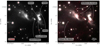 |
Fig. 1 LBT/LUCI images for the S255IR star-forming region. Left panel: adaptive optics assisted Ks band image for the S255IR region displayed in linear scale. The FWHM at the position of the AO guide star is ~0″.06 (see Appendix A for more details). The black circles represent sources reported in Zinchenko et al. (2020), whereas the red squares represent Gaia sources used for astrometric solution. Right panel: RGB AO assisted image with red H2, green Brγ, and blue Ks. The red box indicates the FoV shown in Fig. 2. |
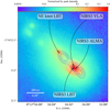 |
Fig. 2 Adaptive optics assisted Ks band image showing zoom-in of the central region of S255IR and featuring NIRS3. The image was normalised to the peak intensity from NIRS3 (labelled NIRS3 LBT) and scaled logarithmically, as shown in the colour bar above the panel. Blue contours represent ALMA band 3 continuum emission with the contour levels [0.5, 1.0, 2.0, 4.0, 5.0, 10.0] ×10−3 Jy beam−1 (Cesaroni et al., in prep.). White contours show VLA 1.3 cm emission with the contour levels [0.8,2.0,5.0,10.0,13.2] ×10−3 Jy beam−1 from Cesaroni et al. (2018). Black circles represent the peak position for NIRS3 and the NE knot for LBT, ALMA, and VLA, as labelled. |
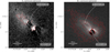 |
Fig. 3 Continuum-subtracted images for the surrounding region of the outbursting source NIRS3. Left panel: H2 continuum-subtracted image. Right panel: Brγ continuum-subtracted image. The red contours represent emission at 3, 5, and 10×RMS, where RMS is the root mean square for each image. The white contours are ALMA band 3 continuum emission, and the contours levels are [0.5, 1.0, 2.0, 4.0, 5.0, 10.0] ×10−3 Jy beam−1. |
3.2 Thirty-year photometric variability of NIRS3
Variability in low-mass YSOs has been observed in many systems (see, e.g. Herbig 1977; Hartmann & Kenyon 1996; MacFarlane et al. 2019; Zakri et al. 2022) and has also been simulated (Zhu et al. 2009; Stamatellos et al. 2011, 2012). (See Fischer et al. 2022 for a recent review.) This variability has many origins; one of which is accretion variability giving rise to outbursts. However, accretion variability in high-mass protostars is less explored, and there are only a handful of observed examples (Caratti o Garatti et al. 2017; Hunter et al. 2017; Stecklum et al. 2021; Chen et al. 2021). Three-dimensional simulations have recently addressed the episodic accretion scenario in HMYSOs (Elbakyan et al. 2023). These simulations suggest that high-density post-collapse clumps crossing the inner computational boundary could give rise to observable outbursts.
Caratti o Garatti et al. (2017) reported the accretion outburst of NIRS3 by comparing a pre-outburst image from UKIDSS with a (post)outburst image from PANIC (Stecklum et al. 2016), dated 8 December 2009 and 28 November 2015, respectively. The authors measured a large increase in both the H and K bands by ∆H ~ 3.5 mag and ∆K ~ 2.5 mag. There was a simultaneous flaring of the 6.7 GHz methanol masers (Fujisawa et al. 2015). Soon after, Uchiyama et al. (2020) performed an NIR follow-up of NIRS3 and measured the photometry from November 2015 to March 2019, measuring the maximum brightness in December 2015 with K = 8.03 ± 0.05 mag. The authors discussed that in the ~4.5 yr baseline of observations, they only detected one episodic event. However, we have gathered photometry from the late 1980s to the early 2000s, and we speculate that another episodic event took place in the late 1980s, as Tamura et al. (1991) measured a K = 10.1 mag in NIRS3 in May 1989, although the authors state the poor accuracy of this photometric point that may be caused by contamination of nearby sources. Additionally, Hodapp (1994) observed this region in February 1991, and we performed aperture photometry on their images, obtaining K = 11.49 ± 0.03 mag. Howard et al. (1997) and Miralles et al. (1997) reported K = 11.08 mag in February 1994 and K = 11.31 mag in February 1996, respectively, for NIRS3. Later, in February 1999, Bik (2004) reported K = 12.56 mag, which seems to indicate the minimum of this alleged previous outburst. Only a year later, in 2000, Itoh et al. (2001) and Ojha et al. (2011) reported K = 12.01 mag and K = 11.82 mag, respectively, indicating that the previous photometric point was likely a minimum. Although the photometric dataset is not homogeneous and the observations were taken with different instruments and conditions, this dataset hints at the fact that NIRS3 is highly variable.
In our AO assisted images, we performed photometry at the position of NIRS3 (see Table A.1 for exact coordinates used). Here, we report two values for our 2022 epoch: one with an aperture radius of 1″, in order to compare the value with previous studies, and the other with a radius of ~2 × FWHM ~ 0″.15 to avoid scattered light from the surrounding medium (see Fig. B.1). In the first case, we measured K1″ = 12.37 ± 0.06 mag, whereas in the second we obtained K0″.15 = 13.48 ± 0.06 mag. The source NIRS3 seems to be in its dimmest state in the historic series. The photometry was performed using the tool SedFluxer from sedcreator (Fedriani et al. 2023), see Appendix B for more details. Figure 4 shows the K band photometry for NIRS3 from 1989 to 2022. The approximately 30 yr of photometry for NIRS3 suggests that in addition to the 2015 outburst, there may have been another in the late 1980s (indicated with red dashed and red dashed-dotted lines in the figure). The amplitude of the first episode is ∆K ≳ −2.5 mag. The quiescent phase then lasted about 10 yr, as the UKIDSS photometric point started to raise with respect to that of Itoh et al. (2001). After that, NIRS3 underwent the confirmed outburst (Fujisawa et al. 2015; Stecklum et al. 2016; Caratti o Garatti et al. 2017) with an amplitude of ∆K ~ 3.37 mag, considering the UKIDSS photometry and the maximum of Uchiyama et al. (2020). After a further 7 yr, the NIR K magnitude dropped by ∆K ~ −4.34 mag (or ∆K ~ −5.45 mag, if we consider K0″.15) from the maximum in Uchiyama et al. (2020). To the best of our knowledge, this is the largest amplitude episode ever registered for NIRS3 and for any high-mass protostar in the K band (assuming that the visual extinction towards the source did not dramatically change). Notably, the time span between the bright and dim states would be similar in both episodic events (i.e. ~6–10 yr). Table B.1 summarises the photometric points discussed above and presented in Fig. 4.
Although there are no methanol maser observations at the time of the alleged first outburst (late 1980s), we note that the NIR photometric variability seen in the 1990s is consistent with the maser variability reported in the same period. Caswell et al. (1995) reported a 10% variability in the methanol maser between 1992 and 1993 and an increase by a factor of ten of the feature at 1.8 km s−1. This is a remarkable change in methanol maser activity, as these masers do not usually change by a factor of ten. For context, Szymczak et al. (2018a) performed monitoring of methanol masers in 139 star-forming sites and reported that 80% of the sources display variability greater than 10%. They discussed the scenario of short-lived outbursts for those sites with a relative amplitude greater than two. Moreover, as part of the long-term programme, Szymczak et al. (2018b) presented methanol maser observations for S255IR NIRS3, including previous works by Menten (1991), Caswell et al. (1995), Szymczak & Kus (2000), Goedhart et al. (2004), and Szymczak et al. (2012). Szymczak et al. (2018b) showed the available flux measurements of the methanol maser from 1991 to 2017 (see their Fig. 2), a period that does not cover the alleged outburst in the late 1980s. However, we note that changes in the pumping radiation due to episodic accretion are only one of the possible reasons for maser flux variability. Therefore, it seems possible that from the late 1980s to the early 2000s, there have been fluctuations in the accretion rate onto the protostar as suggested by the NIR photometric and methanol maser variability. The earlier NIR observations by Strom et al. (1976) and Evans et al. (1977) do not report photometric measurements for NIRS3, and thus they cannot be used to confirm the existence of an outburst.
Burns et al. (2016) proposed that at least three episodes of ejections have taken place in NIRS3 (which they refer to as SMA1) in the last few thousand years. The signature of one of these ejection episodes was observed by Wang et al. (2010) and Zinchenko et al. (2015) in the form of [FeII] and HCO+ jet knots, respectively, with a dynamic age of ~1000 yr. The observed NIRS3 H2 knots indicated by the white arrows in the right panel of Fig. 1 would be part of this episode, as their dynamic age is similar (400–700 yr; see Sect. 3). The most recent ejection episode is then our radio and NIR ‘NE knot LBT’, with just 7 yr of dynamic age (see Figs. 1 and 3).
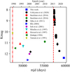 |
Fig. 4 Photometry for S255IR NIRS3 source. The lower x-axis is in units of modified Julian date (mjd) in days, and the upper x-axis gives the date. Errors are also plotted, but some of them are smaller than the symbol used. The red dashed-dotted line represents the alleged outburst that occurred in the late 1980s, whereas the red dashed line marks the confirmed outburst registered in June 2015. |
4 Conclusions
We observed the high-mass star-forming region S255IR using the LBT with the LUCI instrument in the AO assisted imaging mode, achieving an angular resolution of ~0″.06. The region S255IR harbours the outbursting source NIRS3, which underwent an accretion outburst in 2015 and has since faded. The photometry measured in this work yielded the faintest minimum to date for NIRS3, with K0″.15 = 13.48 mag, indicating that the source is in a quiescent state.
We observed a new knot to the north-east of NIRS3 that we interpret as a jet knot ejected during the latest accretion outburst. We measured a tangential velocity of 450 ± 50 km s−1 for this knot. This emission is consistent with previous radio observations made with the VLA and ALMA tracing the outflowing material. In the H2 continuum-subtracted image, we identified extended, elongated emission consistent with jet-shocked material. However, as shown in our Brγ continuum-subtracted image, this extended emission was more likely to be scattered light from a combination of the accretion activity and the UV radiation from the massive protostar NIRS3.
We speculate that NIRS3 has undergone two outbursts in the last 30 yr. If this is true, NIRS3 would be the first massive protostar with at least two outbursts observed in the NIR. Although we cannot thoroughly confirm the first burst, the high photometric variability (along with other accretion-burst tracers) suggests that NIRS3 is in a very active accretion stage prone to more accretion bursts.
Acknowledgements
The authors acknowledge fruitful discussions with G. MacLeod and R. Burns. R.F. acknowledges support from the grants Juan de la Cierva FJC2021-046802-I, PID2020-114461GB-I00 and CEX2021-001131-S funded by MCIN/AEI/10.13039/501100011033 and by “European Union NextGenerationEU/PRTR” and grant P20-00880 from the Consejería de Transformación Económica, Industria, Conocimiento y Universidades of the Junta de Andalucía. R.F. also acknowledges funding from the European Union’s Horizon 2020 research and innovation programme under the Marie Sklodowska-Curie grant agreement No 101032092. A.C.G. has been supported by PRIN-INAF-MAIN-STREAM 2017 “Protoplanetary disks seen through the eyes of new-generation instruments” and by PRIN-INAF 2019 “Spectroscopically tracing the disk dispersal evolution (STRADE)”. J.C.T. acknowledges support from ERC grant MSTAR, VR grant 2017-04522, and NSF grant 1910675. G.C. acknowledges support from the Swedish Research Council (VR Grant; Project: 2021-05589).
Appendix A SOUL performance
To retrieve the FWHM in our images, we fit a Moffat profile (Moffat 1969) along the x and y axes of the image. The point spread function (PSF) under the assumption of circularity (i.e. azimuthally symmetric) is given by:
![Mathematical equation: ${f_{{\rm{Moffat}}}}\left( r \right) = A{\left[ {1 + {{\left( {{{r - {r_0}} \over R}} \right)}^2}} \right]^{ - \beta }},$](/articles/aa/full_html/2023/08/aa46736-23/aa46736-23-eq2.png) (A.1)
(A.1)
where r is the distance from the centre r0, R is the core width, and β is the power. We fit the Moffat profile along the x and y directions for various sources, including the AO guide star itself (2MASSJ06125505+1759289), the main science target (NIRS3), and the furthest star from the AO guide star common to the three filters. In the top panels of Figure A.1, we show the 1D intensity profile (left panel) and the 2D cutout (right panel) for the AO guide star. We extracted these profiles at the peak intensity pixel. In the bottom panels, we show the Moffat fits as solid red lines. One can see that the Moffat profile fits the wings very well, which are especially important in determining the shape of the PSF. To retrieve the FWHM in the Moffat profile, we used the expression:
 (A.2)
(A.2)
In Table A.1, we summarise the properties of the three representative sources in our region mentioned above. The columns in the table report the FWHM, central coordinates, and distance from the AO guide star as measured from the NIR images. We note that the FWHM is fairly constant among filters for the same source. However, one can see how the FWHM degrades with distance from the AO star. It is also worth noting that even though the NIRS3 region is not the farthest away from the AO guide star, it presents a larger FWHM than the farthest away star. This occurs because at this position, the emission is dominated by extended nebulosity, which increases the FWHM.
SOUL performance of the three representative sources for the three filters used.
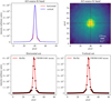 |
Fig. A.1 SOUL performance example featuring the Ks image with the AO guide star used in our observations. Top row: One-dimensional profiles of the horizontal (red) and vertical (blue) cuts (left panel) from the cutout image (right). Bottom row: Moffat fits to the horizontal (left panel) and the vertical (right panel) cuts. The data are shown as black circles and the best fit as red solid lines. |
Appendix B Aperture photometry
We performed circular aperture photometry with the main aperture centred on the central coordinates of NIRS3 (see Table A.1). We selected two apertures and performed two separate photometric measurements. The first had a radius of 1″, in order to compare the data with that of previous studies, and the second had a radius of 0″.15, in order to account for our higher angular resolution (best resolution in the NIR to date for NIRS3). We used the open source Python package sedcreator (Fedriani et al. 2023), in particular the SedFluxer class, to perform aperture photometry. Figure B.1 shows the plot generated by the SedFluxer. The background was estimated from an annulus with inner and outer radii equal to one and two times the radius of the main aperture, represented as red dashed lines in the plots. The background was then considered to be the median value within the annulus multiplied by the area of the main aperture. This background value was then subtracted from the flux obtained in the main aperture. Table B.1 summarises properties of the photometry from the past 30 years.
K band photometry for NIRS3 used in Figure 4 and described in Section 3.2. Table
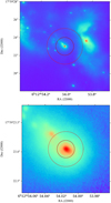 |
Fig. B.1 Zoom-in of a Ks band image of the central region of S255IR. The red cross represents the centre of the aperture, the black circle is the main aperture used, and the red dashed lines are the inner and outer radius of the annulus, which account for the background estimation. We used an aperture radius of 1″ (top panel) and 0″.15 (bottom panel). |
Appendix C Non-annotated figures
In this section, we present the figures used in the main text with the annotations removed. We show Figure C.1, with and without the contours, as well as Figure C.2 so that all the details can be represented. We also present the H2 and Brγ images in Figure C.3.
References
- Astropy Collaboration (Price-Whelan, A. M., et al.) 2018, AJ, 156, 123 [Google Scholar]
- Bally, J. 2016, ARA&A, 54, 491 [Google Scholar]
- Beltrán, M. T., & de Wit, W. J. 2016, A&ARv, 24, 6 [Google Scholar]
- Bik, A. 2004, PhD Thesis, University of Amsterdam, The Netherlands [Google Scholar]
- Boley, P. A., Linz, H., van Boekel, R., et al. 2013, A&A, 558, A24 [NASA ADS] [CrossRef] [EDP Sciences] [Google Scholar]
- Bradley, L., Sipőcz, B., Robitaille, T., et al. 2020, https://doi.org/10.5281/zenodo.4044744 [Google Scholar]
- Burns, R. A., Handa, T., Nagayama, T., Sunada, K., & Omodaka, T. 2016, MNRAS, 460, 283 [NASA ADS] [CrossRef] [Google Scholar]
- Cabrit, S. 2007, in IAU Symposium, 243, 203 [NASA ADS] [CrossRef] [Google Scholar]
- Caratti o Garatti, A., Stecklum, B., Garcia Lopez, R., et al. 2017, Nat. Phys., 13, 276 [Google Scholar]
- Caswell, J. L., Vaile, R. A., & Ellingsen, S. P. 1995, PASA, 12, 37 [NASA ADS] [Google Scholar]
- Cesaroni, R., Moscadelli, L., Neri, R., et al. 2018, A&A, 612, A103 [NASA ADS] [CrossRef] [EDP Sciences] [Google Scholar]
- Chen, Z., Sun, W., Chini, R., et al. 2021, ApJ, 922, 90 [NASA ADS] [CrossRef] [Google Scholar]
- Craig, M., Crawford, S., Seifert, M., et al. 2022, https://doi.org/10.5281/zenodo.6533213 [Google Scholar]
- Elbakyan, V. G., Nayakshin, S., Meyer, D. M. A., & Vorobyov, E. I. 2023, MNRAS, 518, 791 [Google Scholar]
- Evans, N. J. I., Blair, G. N., & Beckwith, S. 1977, ApJ, 217, 448 [NASA ADS] [CrossRef] [Google Scholar]
- Fedriani, R., Caratti o Garatti, A., Coffey, D., et al. 2018, A&A, 616, A126 [NASA ADS] [CrossRef] [EDP Sciences] [Google Scholar]
- Fedriani, R., Garatti, A. C. O., Purser, S. J. D., et al. 2019, Nat. Commun., 10, 3630 [NASA ADS] [CrossRef] [Google Scholar]
- Fedriani, R., Tan, J. C., Telkamp, Z., et al. 2023, ApJ, 942, 7 [NASA ADS] [CrossRef] [Google Scholar]
- Fischer, W. J., Hillenbrand, L. A., Herczeg, G. J., et al. 2022, arXiv e-prints, [arXiv:2203.11257] [Google Scholar]
- Fujisawa, K., Yonekura, Y., Sugiyama, K., et al. 2015, ATel, 8286, 1 [NASA ADS] [Google Scholar]
- Goedhart, S., Gaylard, M. J., & van der Walt, D. J. 2004, MNRAS, 355, 553 [Google Scholar]
- Hartmann, L., & Kenyon, S. J. 1996, ARA&A, 34, 207 [NASA ADS] [CrossRef] [Google Scholar]
- Herbig, G. H. 1977, ApJ, 217, 693 [NASA ADS] [CrossRef] [Google Scholar]
- Hodapp, K.-W. 1994, ApJS, 94, 615 [Google Scholar]
- Howard, E. M., Pipher, J. L., & Forrest, W. J. 1997, ApJ, 481, 327 [NASA ADS] [CrossRef] [Google Scholar]
- Hunter, T. R., Brogan, C. L., MacLeod, G., et al. 2017, ApJ, 837, L29 [NASA ADS] [CrossRef] [Google Scholar]
- Itoh, Y., Tamura, M., Suto, H., et al. 2001, PASJ, 53, 495 [Google Scholar]
- Lo, K. Y., Burke, B. F., & Haschick, A. D. 1975, ApJ, 202, 81 [NASA ADS] [CrossRef] [Google Scholar]
- MacFarlane, B., Stamatellos, D., Johnstone, D., et al. 2019, MNRAS, 487, 5106 [NASA ADS] [CrossRef] [Google Scholar]
- Massi, F., Caratti o Garatti, A., Cesaroni, R., et al. 2023, A&A, 672, A113 [NASA ADS] [CrossRef] [EDP Sciences] [Google Scholar]
- Menten, K. M. 1991, ApJ, 380, L75 [Google Scholar]
- Miralles, M. P., Salas, L., Cruz-González, I., & Kurtz, S. 1997, ApJ, 488, 749 [NASA ADS] [CrossRef] [Google Scholar]
- Moffat, A. F. J. 1969, A&A, 3, 455 [NASA ADS] [Google Scholar]
- Ojha, D. K., Samal, M. R., Pandey, A. K., et al. 2011, ApJ, 738, 156 [CrossRef] [Google Scholar]
- Pinna, E., Esposito, S., Hinz, P., et al. 2016, in Adaptive Optics Systems V, 9909, (SPIE), 99093V [NASA ADS] [CrossRef] [Google Scholar]
- Snell, R. L., & Bally, J. 1986, ApJ, 303, 683 [NASA ADS] [CrossRef] [Google Scholar]
- Stamatellos, D., Whitworth, A. P., & Hubber, D. A. 2011, ApJ, 730, 32 [Google Scholar]
- Stamatellos, D., Whitworth, A. P., & Hubber, D. A. 2012, MNRAS, 427, 1182 [NASA ADS] [CrossRef] [Google Scholar]
- Stecklum, B., Caratti o Garatti, A., Cardenas, M. C., et al. 2016, Atel, 8732, 1 [NASA ADS] [Google Scholar]
- Stecklum, B., Wolf, V., Linz, H., et al. 2021, A&A, 646, A161 [EDP Sciences] [Google Scholar]
- Strom, K. M., Strom, S. E., & Vrba, F. J. 1976, AJ, 81, 308 [CrossRef] [Google Scholar]
- Szymczak, M., & Kus, A. J. 2000, A&As, 147, 181 [NASA ADS] [CrossRef] [EDP Sciences] [Google Scholar]
- Szymczak, M., Wolak, P., Bartkiewicz, A., & Borkowski, K. M. 2012, Astron. Nachr., 333, 634 [NASA ADS] [CrossRef] [Google Scholar]
- Szymczak, M., Olech, M., Sarniak, R., Wolak, P., & Bartkiewicz, A. 2018a, MNRAS, 474, 219 [Google Scholar]
- Szymczak, M., Olech, M., Wolak, P., Gérard, E., & Bartkiewicz, A. 2018b, A&A, 617, A80 [NASA ADS] [CrossRef] [EDP Sciences] [Google Scholar]
- Tamura, M., Gatley, I., Joyce, R. R., et al. 1991, ApJ, 378, 611 [NASA ADS] [CrossRef] [Google Scholar]
- Tan, J. C., Beltrán, M. T., Caselli, P., et al. 2014, Protostars and Planets VI, 149 [Google Scholar]
- Turner, B. E. 1971, Astrophys. Lett., 8, 73 [NASA ADS] [Google Scholar]
- Uchiyama, M., Yamashita, T., Sugiyama, K., et al. 2020, PASJ, 72, 4 [NASA ADS] [CrossRef] [Google Scholar]
- Wang, P., Li, Z.-Y., Abel, T., & Nakamura, F. 2010, ApJ, 709, 27 [NASA ADS] [CrossRef] [Google Scholar]
- Wang, Y., Beuther, H., Bik, A., et al. 2011, A&A, 527, A32 [NASA ADS] [CrossRef] [EDP Sciences] [Google Scholar]
- Zakri, W., Megeath, S. T., Fischer, W. J., et al. 2022, ApJ, 924, L23 [NASA ADS] [CrossRef] [Google Scholar]
- Zhu, Z., Hartmann, L., & Gammie, C. 2009, ApJ, 694, 1045 [Google Scholar]
- Zinchenko, I., Liu, S. Y., Su, Y. N., et al. 2015, ApJ, 810, 10 [Google Scholar]
- Zinchenko, I. I., Liu, S.-Y., Su, Y.-N., Wang, K.-S., & Wang, Y. 2020, ApJ, 889, 43 [NASA ADS] [CrossRef] [Google Scholar]
- Zinnecker, H., McCaughrean, M. J., & Rayner, J. T. 1998, Nature, 394, 862 [NASA ADS] [CrossRef] [Google Scholar]
All Tables
SOUL performance of the three representative sources for the three filters used.
K band photometry for NIRS3 used in Figure 4 and described in Section 3.2. Table
All Figures
|
Fig. 1 LBT/LUCI images for the S255IR star-forming region. Left panel: adaptive optics assisted Ks band image for the S255IR region displayed in linear scale. The FWHM at the position of the AO guide star is ~0″.06 (see Appendix A for more details). The black circles represent sources reported in Zinchenko et al. (2020), whereas the red squares represent Gaia sources used for astrometric solution. Right panel: RGB AO assisted image with red H2, green Brγ, and blue Ks. The red box indicates the FoV shown in Fig. 2. |
| In the text | |
|
Fig. 2 Adaptive optics assisted Ks band image showing zoom-in of the central region of S255IR and featuring NIRS3. The image was normalised to the peak intensity from NIRS3 (labelled NIRS3 LBT) and scaled logarithmically, as shown in the colour bar above the panel. Blue contours represent ALMA band 3 continuum emission with the contour levels [0.5, 1.0, 2.0, 4.0, 5.0, 10.0] ×10−3 Jy beam−1 (Cesaroni et al., in prep.). White contours show VLA 1.3 cm emission with the contour levels [0.8,2.0,5.0,10.0,13.2] ×10−3 Jy beam−1 from Cesaroni et al. (2018). Black circles represent the peak position for NIRS3 and the NE knot for LBT, ALMA, and VLA, as labelled. |
| In the text | |
|
Fig. 3 Continuum-subtracted images for the surrounding region of the outbursting source NIRS3. Left panel: H2 continuum-subtracted image. Right panel: Brγ continuum-subtracted image. The red contours represent emission at 3, 5, and 10×RMS, where RMS is the root mean square for each image. The white contours are ALMA band 3 continuum emission, and the contours levels are [0.5, 1.0, 2.0, 4.0, 5.0, 10.0] ×10−3 Jy beam−1. |
| In the text | |
|
Fig. 4 Photometry for S255IR NIRS3 source. The lower x-axis is in units of modified Julian date (mjd) in days, and the upper x-axis gives the date. Errors are also plotted, but some of them are smaller than the symbol used. The red dashed-dotted line represents the alleged outburst that occurred in the late 1980s, whereas the red dashed line marks the confirmed outburst registered in June 2015. |
| In the text | |
|
Fig. A.1 SOUL performance example featuring the Ks image with the AO guide star used in our observations. Top row: One-dimensional profiles of the horizontal (red) and vertical (blue) cuts (left panel) from the cutout image (right). Bottom row: Moffat fits to the horizontal (left panel) and the vertical (right panel) cuts. The data are shown as black circles and the best fit as red solid lines. |
| In the text | |
|
Fig. B.1 Zoom-in of a Ks band image of the central region of S255IR. The red cross represents the centre of the aperture, the black circle is the main aperture used, and the red dashed lines are the inner and outer radius of the annulus, which account for the background estimation. We used an aperture radius of 1″ (top panel) and 0″.15 (bottom panel). |
| In the text | |
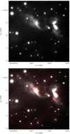 |
Fig. C.1 Same as Figure 1 but with no annotations. |
| In the text | |
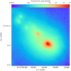 |
Fig. C.2 Same as Figure 2 but with no annotations and no contours. |
| In the text | |
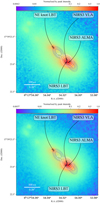 |
Fig. C.3 Same as Figure 2 but for the filters H2 (top panel) and Brγ (bottom panel). |
| In the text | |
Current usage metrics show cumulative count of Article Views (full-text article views including HTML views, PDF and ePub downloads, according to the available data) and Abstracts Views on Vision4Press platform.
Data correspond to usage on the plateform after 2015. The current usage metrics is available 48-96 hours after online publication and is updated daily on week days.
Initial download of the metrics may take a while.