| Issue |
A&A
Volume 680, December 2023
|
|
|---|---|---|
| Article Number | A110 | |
| Number of page(s) | 14 | |
| Section | Interstellar and circumstellar matter | |
| DOI | https://doi.org/10.1051/0004-6361/202347468 | |
| Published online | 19 December 2023 | |
Radio outburst from a massive (proto)star
II. A portrait in space and time of the expanding radio jet from S255IR NIRS 3★
1
INAF, Osservatorio Astrofísico di Arcetri,
Largo E. Fermi 5,
50125
Firenze,
Italy
e-mail: This email address is being protected from spambots. You need JavaScript enabled to view it.
2
INAF, Osservatorio Astronomico di Capodimonte,
via Moiariello 16,
80131
Napoli,
Italy
3
Dublin Institute for Advanced Studies, School of Cosmic Physics, Astronomy & Astrophysics Section,
31 Fitzwilliam Place,
Dublin 2,
Ireland
4
Thüringer Landessternwarte Tautenburg,
Sternwarte 5,
07778
Tautenburg,
Germany
5
Instituto de Astrofísica de Andalucía, CSIC,
Glorieta de la Astronomía s/n,
18008
Granada,
Spain
6
Institut de Radioastronomie Millimétrique (IRAM),
300 rue de la Piscine,
38406
Saint-Martin-d’Hères,
France
7
INAF, Osservatorio Astronomico di Cagliari,
Via della Scienza 5,
09047
Selargius (CA),
Italy
Received:
14
July
2023
Accepted:
17
October
2023
Abstract
Context. Growing observational evidence indicates that the accretion process leading to star formation may occur in an episodic way, through accretion outbursts revealed in various tracers. This phenomenon has also now been detected in association with a few young massive (proto)stars (>8 M⊙), where an increase in the emission has been observed from the IR to the centimetre domain. In particular, the recent outburst at radio wavelengths of S255IR NIRS 3 has been interpreted as due to the expansion of a thermal jet, fed by part of the infalling material, a fraction of which has been converted into an outflow.
Aims. We wish to follow up on our previous study of the centimetre and millimetre continuum emission from the outbursting massive (proto)star S255IR NIRS 3 and confirm our interpretation of the radio outburst, based on an expanding thermal jet.
Methods. The source was monitored for more than 1 yr in six bands from 1.5 GHz to 45.5 GHz with the Karl G. Jansky Very Large Array, and, after an interval of ~1.5 yr, it was imaged with the Atacama Large Millimeter/submillimeter Array at two epochs, which made it possible to detect the proper motions of the jet lobes.
Results. The prediction of our previous study is confirmed by the new results. The radio jet is found to expand, while the flux, after an initial exponential increase, appears to stabilise and eventually decline, albeit very slowly. The radio flux measured during our monitoring is attributed to a single lobe, expanding towards the NE. However, starting from 2019, a second lobe has been emerging in the opposite direction, probably powered by the same accretion outburst as the NE lobe, although with a delay of at least a couple of years. Flux densities measured at frequencies higher than 6 GHz were satisfactorily fitted with a jet model, whereas those below 6 GHz are clearly underestimated by the model. This indicates that non-thermal emission becomes dominant at long wavelengths.
Conclusions. Our results suggest that thermal jets can be a direct consequence of accretion events, when yearly flux variations are detected. The formation of a jet lobe and its early expansion appear to have been triggered by the accretion event that started in 2015. The end of the accretion outburst is also mirrored in the radio jet. In fact, ~1 yr after the onset of the radio outburst, the inner radius of the jet began to increase, at the same time the jet mass stopped growing, as expected if the powering mechanism of the jet is quenched. We conclude that our findings strongly support a tight connection between accretion and ejection in massive stars, consistent with a formation process involving a disk-jet system similar to that of low-mass stars.
Key words: stars: individual: S255IR NIRS3 / stars: early-type / stars: formation / ISM: jets and outflows
Based on observations carried out with the VLA and ALMA.
© The Authors 2023
 Open Access article, published by EDP Sciences, under the terms of the Creative Commons Attribution License (https://creativecommons.org/licenses/by/4.0), which permits unrestricted use, distribution, and reproduction in any medium, provided the original work is properly cited.
This article is published in open access under the Subscribe to Open model. This email address is being protected from spambots. You need JavaScript enabled to view it. to support open access publication.
1 Introduction
In recent years, observations have provided us with increasing evidence of circumstellar rotating structures around B-type (proto)stars, especially since the advent of the Atacama Large Millimeter/submillrmeter Array (ALMA; see e.g. the review by Beltrán & de Wit 2016). This strongly suggests that disk-mediated accretion could be a viable mechanism to feed even the most massive stars. However, we still do not understand the physical properties of these rotating structures, nor how such an accretion proceeds, whether through a smooth, continuous flow or episodically with parcels of material falling onto the star. The recent detection of outbursts (Stecklum 2016, 2021; Caratti o Garatti et al. 2017; Hunter et al. 2017, 2021; Burns et al. 2020, 2023; Chen et al. 2021) in a few luminous young stellar objects (YSOs) >8 M⊙ provides us with the intriguing possibility that these phenomena could be the consequence of episodic accretion events, akin to those commonly observed in low-mass YSOs as FU Orionis and EX Orionis events (Audard et al. 2014; Fischer et al. 2023).
In this study, we focus on the outburst from the massive (proto)star S255IR NIRS 3, located at a distance of  kpc (Burns et al. 2016). This object is unique because the outburst has been observed not only in the emission of some maser species (Fujisawa et al. 2015; Moscadelli et al. 2017; Hirota et al. 2021) and in lines and continua at IR and (sub-)millimetre wavelengths (Caratti o Garatti et al. 2017; Uchiyama et al. 2020; Liu et al. 2018), but also in the centimetre domain (Cesaroni et al. 2018; hereafter Paper I). A time delay of ~1 yr was found between the onset of the IR and radio outbursts, consistent with the different mechanisms at the origin of the two: in fact, the IR outburst is based on radiative processes propagating at velocities comparable to the speed of light, whereas the radio outburst is due to shocks expanding approximately at the speed of sound. In Paper I, we present compelling evidence of an exponential increase in the radio emission from the thermal jet associated with this source. Given the existence of a disk-jet system in S255IR NIRS 3 (Boley et al. 2013; Wang et al. 2011; Zinchenko et al. 2015; Liu et al. 2020), we believe that we are witnessing an episodic accretion event mediated by the disk, where part of the infalling material has been diverted into the associated jet Fedriani et al. (2023). In Paper I, we show that a simple model of an expanding jet can satisfactorily reproduce the increase in the radio flux observed in four bands. Although the emission was basically unresolved, we predicted that in a few years the jet expansion should make it possible to resolve its structure. With this in mind, we performed both monitoring of the radio emission and sub-arcsecond millimetre imaging at two epochs, several years after the beginning of the outburst. In this article we report on the results of these observations.
2 Observations
The radio emission was monitored with the Karl G. Jansky Very Large Array (VLA) and, at a later time, with ALMA. In the following we describe the observational setup and data reduction separately for the two datasets. In both cases, for the phase centre we chose the position α(J2000)=06h 12m 54s.02, δ(J2000)=17° 59′ 23″.1.
2.1 Very large array
S255IR NIRS 3 was observed at 11 epochs from January 2017 to January 2018 (project codes: 16B-427 and 17B-045). The observing dates and array configurations are listed in Table 1, where for the sake of completeness we have also included the 2016 data already presented in Paper I. We note that the table contains as yet unpublished data in the L band obtained in the same observing run (project 16A-424) described in Paper I.
The signal was recorded with the Wideband Interferometric Digital ARchitecture (WIDAR) correlator in six bands, centred approximately at 1.5 (L band), 3 (S), 6 (C), 10 (X), 22.2 (K), and 45.5 GHz (Q), in dual polarisation mode. The total observing bandwidth (per polarisation) was 1 GHz in the L band, 2 GHz in the S band, 4 GHz in the C and X bands, and 8 GHz in the K and Q bands. The primary flux calibrator was 3C48 and the phase-calibrators were J0632+1022 in the L and S bands, J0559+2353 in the C and X bands, and J0539+1433 in the K and Q4 bands.
We made use of the calibrated dataset provided by the NRAO pipeline and subsequent inspection of the data and imaging were performed with the CASA1 package, version 5.6.2-2. The continuum images were constructed using natural weighting to maximise flux recovery. Typical values of the 1σ RMS noise level and synthesised beam are given in Table 2 for each band and array configuration.
The flux density of the compact, variable source centred on S255IR NIRS 3 has been estimated inside a polygonal shape encompassing the compact, unresolved radio source and is given in Table 1 for each band and epoch. As explained in Paper I, in our VLA observations the continuum emission from S255IR NIRS 3 appears as an unresolved component (the variable source of interest for our study) plus two large-scale lobes separated by ~8″, or ~ 15 000 au, in projection (see Fig. 1 of Paper I) that in all likelihood are originating from a previous outburst that occurred many decades ago. At the longest wavelengths it was possible to resolve the central source from the lobes only in the most extended array configuration. In the other cases, we could only measure the total flux density from all components and the corresponding values are reported in Table 1 as upper limits. In a few cases, as indicated in the footnotes of the table, we attempted a correction to the flux, under the assumption that the flux of the lobes is constant in time and thus equal to the value measured (at a different epoch) with the A array. With this approach a caveat is in order, because a compact configuration may be sensitive to lobe structures that are resolved out in a more extended configuration. This implies that the corrected flux densities could be still an upper limit.
In order to estimate the uncertainty on the flux density measurements of S255IR NIRS 3, we took advantage of the presence of a compact, marginally resolved continuum source located approximately at α(J2000) = 06h 12m53s.61, δ(J2000) = 18° 00′ 26″.4, which happens to fall in the primary beam in all bands except band Q. Under the reasonable assumption that this object is not variable, by comparing the flux density measurements obtained at different epochs at the same frequency, we estimated a relative error of 10% in all bands.
2.2 Atacama Large Millimeter/submillimeter Array
S255IR NIRS 3 was observed with ALMA in band 3 on June 6, 2019, and September 3, 2021 (project 2018.1.00864.S, P.I. R. Cesaroni). The main characteristics of the observations are summarised in Table 3. The correlator was configured with 4 units of 2 GHz, in double polarisation, centred at 85.2, 87.2, 97.2, and 99.2 GHz. The spectral resolution is 0.49 MHz (corresponding to ~ 1.5–1.7 km s−1, depending on the frequency), sufficient to identify line-free channels and obtain a measurement of the continuum emission.
The data were calibrated through the ALMA data reduction pipeline. For each 2 GHz correlator unit, we created a data cube using task tclean of CASA, adopting natural weighting and a circular beam of 0″.097 for the first epoch and 0″ 087 for the second one. To create a continuum map for each 2 GHz band, we used the STATCONT software2 developed by Sánchez-Monge et al. (2018). In this way we also obtained cubes of the continuum-subtracted line emission. Finally, the four continuum maps were averaged together to increase the signal-to-noise ratio. The measured fluxes at the two epochs are reported in Table 1.
We note that the derivation of the continuum images described above also provides us with continuum-subtracted channel maps. Although a study of the line emission in this region goes beyond the purposes of this article, in the following we briefly consider the maps of two molecular transitions, SO(22−11) at 86093.983 MHz and H13CN(1−0) at 86338.7 MHz.
Flux densities of S255IR NIRS 3 observed at different epochs and frequencies.
3 Results
3.1 Continuum emission at λ=3 mm
The structure of the radio jet from S255IR NIRS 3 at the two epochs observed with ALMA is shown in Fig. 1. The most striking result is the clear expansion of the jet, which becomes significantly more elongated to both the NE and SW. At first look, the figure seems to outline a bipolar structure, where the star might be located close to the geometrical centre, between the two jet lobes. However, this is not the case. Careful comparison between Figs. 1a and b reveals that, while the NE peak is moving away from the centre, the SW peak stays still, consistent with this being the location of the (proto)star. This result is confirmed by the coincidence of the SW peak with the peak of the submillimetre emission (white cross) measured by Liu et al. (2020), as expected if the (proto)star lies inside the parental molecular, dusty core. Figure 2 clearly confirms this scenario by showing an overlay of the molecular emission maps of the SO(22−11) and H13CN(1−0) lines observed by us, with an image of the 3 mm continuum emission. It is worth noting that in both transitions a dip is seen towards the continuum peak, which suggests that part of the line emission is likely absorbed against the bright continuum. This is consistent with the high brightness temperature of both 3 mm continuum peaks, of the order of 500 K (obtained from the maps cleaned with uniform weighting).
With all the above in mind, in the following we assume that the (proto)star powering the radio jet is located at the SW peak of the 3 mm continuum emission, namely at α(J2000) = 06h 12m 54s.012, δ(J2000) = 17° 59′ 23″.04. We prefer to use the peak position of our maps instead of that of the sub-millimetre maps of Liu et al. (2020), because of the higher angular resolution (0″.087 instead of 0″.14).
It is also interesting to compare the jet lobes observed in our ALMA maps with those seen on a much larger scale (see Fig. 1 of Paper I). The comparison is presented in Fig. 3, where we show the maps of the 3.6 cm and 3 mm continuum emission. Clearly, the directions of the symmetry axes of the two pairs of lobes are remarkably different, with position angle (PA) of ~70°, on the large scale, and ~48°, on the small scale. The fact that the two axes have different orientations and do not intersect at the position of the star (i.e. at the SW peak of the 3 mm continuum) can be interpreted in two ways: either we are dealing with two jets originating from two different YSOs, or the jet is precessing and the star is moving on the plane of the sky at a different speed with respect to the large-scale lobes. The latter scenario implies that either the star or the ejected material is experiencing deceleration or acceleration, such that one of the two is lagging behind the other.
Although it is impossible to rule out one of the two hypotheses, in the following we assume that all lobes belong to the same jet, because there is only one core lying along the jet axis and evidence for precession has been found in S255IR NIRS 3 (Wang et al. 2011; Fedriani et al. 2023), as well as other similar objects (see e.g. Shepherd et al. 2000, Cesaroni et al. 2005, Sánchez-Monge et al. 2014, Beltrán et al. 2016). Further support for this hypothesis is given by the progressive change of the position angle of the jet from the large to the small scale, as shown in Table 4. This trend is indeed consistent with a jet outflow undergoing precession.
Typical 1σ RMS noise and synthesised beam for different bands and VLA configurations.
Main parameters of the ALMA observations.
Position angles of the jet outflow from S255IR NIRS 3 in different tracers.
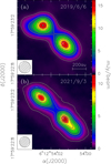 |
Fig. 1 Maps of the 3 mm continuum emission obtained with ALMA. (a) Data acquired on June 6, 2019. Contour levels range from 0.52 to 16.12 in steps of 2.6 mJy beam−1. The cross marks the peak of the 900 μm continuum emission imaged by Liu et al. (2020). The circle in the bottom left represents the synthesised beam. (b) Same as the top panel, but for the map obtained on September 3, 2021. Contour levels range from 0.29 to 16.24 in steps of 1.45 mJy beam−1. |
3.2 Continuum emission at λ ≥ 7 mm
In Fig. 4, we present the continuum spectra obtained from the flux densities in Table 1. Our VLA observations of S255IR NIRS 3 span an interval of time prior to the ALMA observations (see Table 1) and the radio emission of the variable source in S255IR NIRS 3 is basically unresolved in all of our VLA observations. However, we can study the spatial evolution of the jet by determining the position of the peak at different times. For this purpose we fitted a 2D Gaussian to the K-band maps with sub-arcsecond resolution. We prefer the 1.3 cm data to the 7 mm data, which would provide us with better resolution, because in the K band the S/N is higher and in the Q band contamination by dust thermal emission might be present. In Fig. 5, we plot the distribution of the peak positions thus obtained. To give an idea of the uncertainty on these positions, we also draw ellipses corresponding to one-fifth of the synthesised beams. For our analysis we also included the NE peak of our ALMA data and that of Obonyo et al. (2021; hereafter OLHKP). Despite the large uncertainties, it is clear that the distance of the peak from the star is increasing with time, as expected if the jet is expanding. This expansion appears to slow down with time, because the mean velocity (projected on the plane of the sky) estimated from the ratio between the separation of the peaks at the last two epochs (ALMA data) and the corresponding time interval is ~40 au/820 days ≃ 84 km s−1, much less than the mean velocity from the beginning of the radio burst, namely ~472 au/1881 days ≃ 436 km s−1, where ~472 au is the distance of the NE peak from the star at the last epoch. Using the same approach, Fedriani et al. (2023) estimated an expansion speed of 450 ± 50 km s−1 from their IR data. We further analyse the expansion of the jet in Sect. 4.3.1.
The flux density of S255IR NIRS 3 is changing with time in all bands, as shown in Fig. 6. One can identify two phases: the first when the flux increases exponentially for ~200 days; the second when the flux remains basically constant, or slightly declines towards the end of our monitoring. This behaviour is the same at all frequencies ≥6 GHz, but is not so obvious at the two longest wavelengths, where a precise estimate of the flux density of the compact variable source is not possible for the reason explained in Sect. 2.1. Moreover, in these bands our monitoring is more limited in time. It is hence quite possible that the flux density below 6 GHz has a different behaviour than that at higher frequencies. Therefore, the radio emission at 1.5 and 3 GHz, and probably also part of the 6 GHz flux, might not be due to free-free radiation but to another mechanism, such as synchrotron emission, which has been detected towards a number of extended radio jets from YSOs (e.g. Carraco-González et al. 2010; Moscadelli et al. 2013; Brogan et al. 2018; Sanna et al. 2019 and references therein). The evident change of slope in some of the VLA spectra seems to support this possibility. In this respect, the most representative is the spectrum acquired on 2016/10/15 (see Fig. 4), where the 1.5 GHz point lies well above any plausible extrapolation of the other fluxes. For all these reasons, in the following we focus our study on the emission above 6 GHz, with the caveat that even the 6 GHz flux might be partly contaminated by a non-thermal contribution, as suggested by OLHKP. It is worth noting that the existence of synchrotron emission from S255IR NIRS 3 is supported by the recent possible detection of high-energy gamma-ray emission from this source (see de Ona Wilhelmi et al. 2023).
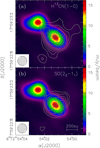 |
Fig. 2 Maps of the line emission obtained with ALMA. (a) Map of the emission averaged over the H13CN(1−0) line (white contours) overlaid on the continuum image at 3 mm obtained on June 6, 2019. Contour levels range from 1.2 to 4.56 in steps of 0.48 mJy beam−1. The circle in the bottom left represents the synthesised beam. (b) Same as the top panel, but for the SO(22−11) line. Contour levels range from 1.65 to 4.62 in steps of 0.33 mJy beam−1. |
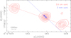 |
Fig. 3 Maps of the 3.6 cm continuum emission obtained with the VLA on July 10, 2016 (red) and of the 3 mm continuum emission (blue), also shown in Fig. 1b. The dashed lines denote the symmetry axes of the bipolar structures. Red contour levels range from 0.1 to 0.6 in steps of 0.1 mJy beam−1. Blue contour levels range from 0.29 to 8.99 in steps of 2.9 mJy beam−1. |
4 Analysis and discussion
4.1 Nature of the 3 mm continuum emission
For the reasons presented in Sect. 3.1, we have concluded that the (proto)star should lie at the SW peak of the 3 mm continuum map. If this is the case, one expects this peak to have a significant contribution from thermal dust emission, whereas the NE peak, being part of a jet lobe, should be dominated by free-free emission. To investigate these assumptions, we computed the spectral index of the 3 mm continuum over the maps in Fig. 1. For this purpose, we used the maps obtained from the four correlator units centred at 85.2, 87.2, 97.2, and 99.2 GHz (see Sect. 2.2), created with the same clean beam. For each pixel of the maps, the spectral index was computed from a least-square fit to the four fluxes in a log Sv−log v plot. The fit was performed only in those pixels where all of the four fluxes were above the 5σ level. The result is shown in Fig. 7, where the formal error obtained from the fit ranges from 0.03 towards the emission peaks to 0.3 towards the borders.
At 3 mm it is reasonable to assume that dust emission is optically thin and the flux density is ∝ vγ, with γ = 2−4, because the dust absorption coefficient is believed to vary as vβ with β = 0−2 (see e.g. D’Alessio et al. 2001; Sadavoy et al. 2013), where β = 0 corresponds to the case of large grains (‘pebbles’) in disks (Testi et al. 2014). The same assumption also holds for the free-free emission: the spectra in Fig. 4 flatten beyond 45 GHz, and hence the flux density is ∝ v−0.1. Therefore, more positive spectral indices can be associated with dust emission and, conversely, more negative ones with free-free emission. At both epochs dust emission arises from the region around the SW peak, as expected for a deeply embedded star, while the NE lobe of the jet is characterised by free-free emission. Noticeably, some free-free emission is also detected towards the most south-western tip.
When estimating the flux density at wavelengths of 3 mm or shorter, it is thus necessary to distinguish between the NE lobe and the rest of the source. In Table 5 we give all these fluxes for the two epochs of the ALMA observations. It is worth pointing out that the spectral index over the SW region is mostly ≲2, whereas the typical index expected for pure dust emission, should lie approximately between 2 and 4. This suggests the presence of non-negligible free-free emission around the SW peak as well. It is possible to estimate what fraction of the total flux is due to free-free as follows. The total flux can be written as  , where
  is the optically thin free-free flux and
  , with γ = 2−4, is the dust flux. As previously explained, the spectral index between v1 = 85.2 GHz and v2 = 99.2 GHz was estimated assuming Sv ∝ vα, and hence we have
 (1)
(1)
 (2)
(2)
After some algebra, we obtain the ratio
 (3)
(3)
and, from this, the fraction of the total flux due to free-free emission, RS/(1 + RS). Using the values of α in Fig. 7, we find that such a fraction on average ranges from 65%, for γ=2, to 85%, for γ=4. This implies that 15–20 mJy out of 23 mJy emitted by the SW component (see Table 5), are contributed by free-free emission, also consistent with the brightness temperature of ~500 K measured at 3 mm towards the SW peak, probably too large to be due only to dust emission. We note that part of this free-free emission might be due to ionisation by the embedded star of ~20 M⊙ (Zinchenko et al. 2015).
As already mentioned, some free-free emission is also detected towards the tip of the SW region and becomes more prominent and more extended with time, as one can see by comparing Figs. 1a to b. This hints at the existence of another jet lobe emerging from the dusty core and expanding towards the SW.
To shed light on the nature of this putative lobe and set a constraint on its age, in Fig. 8 we compare the jet structure observed by OLHKP at 1.3 cm on May 5, 2018, with our ALMA image at 3 mm. It seems that during the period of our monitoring, up to the observation of OLHKP (664 days after the onset of the radio outburst), no significant free-free emission was seen to the SW of the (proto)star at any of the wavelengths observed with the VLA. We thus conclude that in all likelihood the SW jet lobe appeared only recently, between May 2018 and June 2019. Therefore, the radio flux variations monitored by us until January 2018 are to be attributed only to the NE lobe.
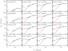 |
Fig. 4 Continuum spectra of the variable, compact component in S255IR NIRS 3. The date of the observations is given in the top left of each panel. The vertical error bars assume a calibration error of 10% in all bands, while the horizontal bars indicate the bandwidth covered at each frequency. The upper limits denote that the flux density is also contributed by the emission from the large-scale lobes, due to the limited angular resolution. Red symbols mark data in the L (1.5 GHz) and S (3 GHz) bands. The curves are the best fits obtained with the model of a thermal jet described in Sect. 4.3.2. |
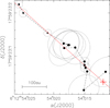 |
Fig. 5 Distribution of the peaks of the 3 mm and 1.3 cm continuum maps obtained, respectively, with ALMA and with the A and B configurations of the VLA. The circles indicate our VLA data, the triangle the data of OLHKP, and the two squares our ALMA data. The dashed line connects the points in order of time (the first point in the bottom-right corner corresponds to the observation on July 10, 2016). The third point from the top left is obtained from the OLHKP data. The cross marks the position of the (proto)star, and the solid red line is the axis of the radio jet (PA = 48°). The dotted ellipses are the synthesised beams scaled down by a factor of 5. |
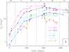 |
Fig. 6 Flux density of the variable, compact source in S255IR NIRS 3 as a function of time from the beginning of the radio burst (July 10, 2016) in all bands observed with the VLA. The two rightmost points are the measurements at 6 and 22 GHz by OLHKP. Curves are colour-coded by frequency (in gigahertz). Arrows denote points with upper limits (see Sect. 2.1), which are connected by dashed lines. The two black arrows pointing to the right indicate the flux densities at 92 GHz of the NE lobe (see Table 1) measured 1061 and 1881 days after the radio burst. Typical error bars are shown in the bottom right of the figure. The vertical dotted lines mark the beginning and end of an array configuration, as labelled above the figure. |
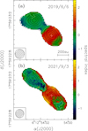 |
Fig. 7 Maps of the 3 mm continuum emission (contours) overlaid on the corresponding map of the spectral index at 3 mm. (a) Data obtained with ALMA on June 6, 2019. Black contour levels range from 10% to 90% in steps of 10% of the peak emission. White contour levels correspond to a spectral index equal to 0. The cross marks the position of the (proto)star. The circle in the bottom left represents the synthesised beam. (b) Same as the top panel, but for the map obtained on September 3, 2021. |
Flux densities in millijanskys measured at 92.5 GHz with ALMA towards the NE and SW components of S255IR NIRS 3.
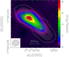 |
Fig. 8 Map of the 3 mm continuum emission obtained with ALMA on September 3, 2021, overlaid on the 1.3 cm image obtained by OLHKP on May 5, 2018. Contour levels are the same as in Fig. 1b. The cross marks the position of the (proto)star. The ellipse in the bottom left represents the synthesised beam at 1.3 cm. |
4.2 Origin of the SW lobe
One may wonder if the emerging SW lobe corresponds to a new radio burst or is somehow related to the accretion outburst observed by Caratti o Garatti et al. (2017). Only follow-up observations of the jet structure will allow us to establish if the new lobe is as prominent and long-lasting as the NE one. However, we point out that the IR monitoring performed by Uchiyama et al. (2020) and Fedriani et al. (2023) between November 2015 and February 2022 as well as the methanol maser observations3 of the Maser Monitoring Organization (M2O)4 have not revealed any other burst after that of Caratti o Garatti et al. (2017) and before the ejection of the SW lobe. We conclude that both jet lobes could arise from the same accretion event, although with a time lag between them of 22–35 months.
This hypothesis is also supported by a noticeable feature of the jet system in S255IR NIRS 3, namely that the extension of the NE lobe is about twice as much as that of the SW lobe. This is true not only for the large-scale and small-scale lobes in Fig. 3, but also for the H2O masers distribution, as shown in Fig. 9. The existence of the same asymmetry on different scales and tracers cannot be a coincidence and is suggestive of a mechanism that causes a delay of the ejection of the SW lobe with respect to the NE lobe. In our opinion, two explanations are possible: either the accretion (and hence ejection) event is intrinsically stronger on the NE side of the disk, or the expansion towards the SW is hindered by the presence of denser material. We favour the latter hypothesis since the near-IR emission is much fainter from the SW lobe than from the NE lobe (see Caratti o Garatti et al. 2017 and Fedriani et al. 2023). This finding is surprising, because the SW lobe corresponds to the blue-shifted emission of the jet outflow (see Wang et al. 2011), which means that the jet is pointing towards the observer on that side and the extinction should be lower than on the NE side. The weakness of the IR emission to the SW is thus indicative of an asymmetry in the density distribution along the jet axis, a fact that could naturally also explain the delay of the expansion of the SW lobe with respect to the NE lobe.
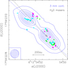 |
Fig. 9 Water masers spots (solid circles) observed by Goddi et al. (2007; cyan), Burns et al. (2016; green), and Hirota et al. (2021; magenta) overlaid on the 3 mm continuum map (blue contours) of Fig. 1b. The dashed lines indicate the jet axes in the two tracers. The cross marks the position of the (proto)star. The circle in the bottom left represents the synthesised beam at 3 mm. |
4.3 Evolution of the radio emission
In this section, we present a model fit to the observed spectra, following the approach adopted in Paper I, with some modifications. As done in Paper I, we adopted the ‘standard spherical’ model from (Reynolds 1986, see his Table 1) to describe the radio continuum emission from the jet. In practice, this means that we assume a jet where at a given time the opening angle, electron temperature, ionisation degree, and expansion speed do not depend on the distance from the star, r.
4.3.1 Expansion law of the jet
In Paper I, the jet was assumed to undergo expansion at constant velocity so that the maximum radius could be described by the simple expression rm(t) = rm(0) + v0t, with v0 = 900 km s−1. While this assumption could hold for the first few months after the onset of the radio outburst, it is inconsistent with the most recent data. In fact, in Sect. 3.2 we show that the jet expansion is slowing down with time. We thus need to adopt a more realistic law for rm(t).
For this purpose, we assume that the jet is expanding in a medium with density ∝ r−2, with r the distance from the star. It is possible to demonstrate (see Appendix A) that applying momentum conservation one obtains
 (4)
(4)
where we have multiplied both terms of Eq. (A.3) by cos ψ, with ψ the angle between the jet axis and the plane of the sky. For consistency with Reynolds (1986), we have indicated with y the projection of r on the plane of the sky. Here, T is a suitable timescale, and v0 and ym0 are, respectively, the expansion velocity and the value of ym at the onset of the radio outburst (i.e. on July 10, 2016). As in Paper I, we chose v0 = 900 km s−1, while the two parameters T and ym0 can be determined from the values of ym estimated from the two ALMA maps at t = 1061 days and t =1881 days.
The problem is that ym cannot be trivially obtained from the position of the NE peak, which corresponds to the maximum brightness temperature. This temperature is attained either at the inner radius, if the whole jet is optically thin, or at the border between the optically thin and the optically thick parts of the jet (denoted by y1 in Reynolds’ notation). Beyond this point, the emission is optically thin and the brightness temperature scales with the opacity τ ∝ r−3, as from Reynolds’ Eq. (4). For this reason, the jet can extend much beyond the position of the observed peak.
In order to obtain a reliable estimate of ym, we have fitted the NE lobe in the two ALMA maps of Fig. 1 assuming that the 3 mm emission is optically thin all over the jet surface. Under this hypothesis the brightness temperature can be expressed as
 (5)
(5)
where y = r cos ψ is the projection of r on the plane of the sky and y0 = r0 cos ψ with r0 the inner radius of the jet. For a given set of y0, ym, and θ0 (the opening angle of the jet) a map was generated, convolved with the instrumental beam, and the model brightness temperature was computed for each pixel of the observed map. The best fit was obtained by minimising the expression
 (6)
(6)
with i a generic pixel, after varying the three parameters over suitable ranges. The best-fit models are compared to the observed maps in Fig. 10 and correspond to θ0 = 9°, y0=0″.206=367 au, and ym=0″.29=516 au, for the first map, and θ0=2°4, y0=0″.207=368 au, and ym=0″.356=634 au, for the second map.
From Eq. (4) written for t=1061 days and t=1881 days, one obtains a system of two equations in the two unknowns T and ym0, the solutions to which are T = 124 days and ym0 = 251 au. Hence, one has
 (7)
(7)
The value of rm can be computed from Eq. (4) assuming ψ =10° (see Paper I, where the complementary angle i = 90° − ψ = 80° was used). Figure 11 compares our solution, ym, as a function of time (blue curve) with (i) the positions of the maximum brightness temperature (the same as in Fig. 5) and (ii) the value of y1 obtained from the model fits described later in Sect. 4.3.2. The latter corresponds to the border between the optically thin and optically thick parts of the jet. Clearly, the brightness appears to peak much closer to y1 than to ym, as previously mentioned.
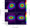 |
Fig. 10 Comparison between the observed maps of the NE lobe of the radio jet (left panels) with the best-fit maps obtained with the model (right panels). The top panels correspond to the first ALMA epoch, bottom panels to the second one. The horizontal axis is parallel to the jet axis. Contour levels range from 10% to 90% in steps of 10% of the peak of each image. The circle in the bottom left represents the synthesised beam. |
4.3.2 Modelling the jet variability
We wish to reproduce the spectral variation shown in Fig. 4 and thus derive the values of the jet parameters as a function of time. For this purpose, we introduce some modifications with respect to the original model by Reynolds (1986), which was used in Paper I. Reynolds’ equations were derived under the approximation of small θ0, the opening angle of the jet5. However, in Paper I we find that θ0 ≃ 20°−50° is needed to fit the spectra. In order to overcome this limitation we re-wrote Reynolds’ equations under suitable assumptions, as detailed in Appendix B, so that they are now valid for any θ0 < 90°.
All observed spectra have been fitted with Eq. (B.9) using only the measurements with v ≥ 6 GHz, for the reasons discussed in Sect. 3.2. We stress that, unlike Paper I, here we assume the jet to be mono-polar, because there is no hint of the existence of a SW lobe during the whole period of our VLA monitoring (see Sect. 4.1). The input parameters of the model are the angle between the jet axis and the plane of the sky, ψ, the ionised gas temperature, T0, the inner radius, r0, the projection of the outer radius on the plane of the sky, ym, the opening angle, θ0, and the parameter  , where x0 is the fraction of ionised gas, v0 the expansion velocity, and
  the total mass loss rate (neutral plus ionised). The quantities T0, v0, and x0 are assumed to be constant along the jet, while T0 is also constant in time.
To simplify the fitting procedure as much as possible, we fixed T0 = 104 K and ψ = 10° (see Paper I), and computed ym from Eq. (7). Unlike in Paper I, we decided to leave r0 free, because a priori the inner radius could change while the jet is expanding. So, we are left with three free parameters: r0, θ0, and Λ. The best fit to each spectrum has been obtained by minimising the χ2 given in Eq. (10) of Paper I, after varying the parameters over the ranges θ0 = 3°−50°, r0 = 50−300 au, and Λ = 10−10−10−7 M⊙ yr−1 (km s−1)−1. The best-fit spectra are represented by the solid curves in Fig. 4 and the best-fit parameters are given in Table 6. The errors on the parameters have been computed using the criterion of Lampton et al. (1976), as done in Paper I.
While most of the fits look to be in agreement with the data within the uncertainties, the 6 GHz fluxes appear to be underestimated by the model at the last five to six epochs. In our opinion, such a discrepancy could indicate contamination from non-thermal emission at this frequency, as already suggested by OLHKP. Indeed, as discussed in Sect. 3.2, non-thermal emission is very prominent at longer wavelengths in the same spectra (red points in Fig. 4) and it is hence not surprising that this type of emission can contribute significantly to the flux up to 6 GHz.
In Fig. 12, we plot the best-fit parameters as a function of time. One sees that the opening angle rapidly increases up to the maximum value allowed by us. It may seem that an opening angle of 50° is too large for a jet, but it is similar to that predicted by theory for a jet powered by a ~20 M⊙ YSO Zinchenko et al. (2015), namely ~52º, obtained by interpolating the values in Table 2 of Staff et al. (2019). Moreover, we can obtain a direct estimate of θ0 from the observed peak brightness temperature in the synthesised beam, TSB, assuming optically thick emission. Approximating the jet as a Gaussian source, one has
 (8)
(8)
where TB is the intrinsic brightness temperature of the source and ΘS and ΘB are, respectively, the full widths at half power of the source and synthesised beam. Consequently,
 (9)
(9)
This expression can be used to calculate a lower limit on the source diameter,  , assuming that the free-free emission is optically thick, namely for TB = T0 = 104 K. Correspondingly, a lower limit on the opening angle is obtained from
 (10)
(10)
where ∆ is the separation between the peak of TSB and the position of the (proto)star. We estimated  for all of our maps, and for each epoch we computed the mean
  obtained from the four bands. This is plotted in Fig. 13 as a function of time. For the sake of comparison we also plot θ0 obtained from our model fits (dashed line). We conclude that, despite the crude approximations adopted to derive Eq. (10), values of θ0 of a few times 10º seem plausible and consistent with our model fit results. It is worth noting that θ0 computed from the map of OLHKP and from our ALMA maps (Fig. 1) using Eq. (10) turns out to be much less, namely 7º, 1º.7, and 1º.3, respectively 664, 1061, and 1881 days after the radio outburst. We speculate that the jet could be re-collimating on a timescale of a couple of years.
Another interesting result from Fig. 12 is the behaviour of r0, which remains basically constant for ~250 days after the radio outburst, thereafter showing a systematic increase until the end of our monitoring – and even beyond that, as we estimate values of ~370 au at the time of our first ALMA observations (see Sect. 4.3.1). A straightforward interpretation is that the inner radius expands when the mechanism feeding the jet is switched off. Noticeably, Λ appears to reach a maximum just when r0 starts increasing, supporting the idea that no more material is added to the jet. This hypothesis is confirmed by Fig. 14, which shows how the ionised jet mass, computed from Eq. (B.13), varies with time. In the same figure we also plot r0 for the sake of comparison. It is quite clear that both quantities have a bi-modal temporal behaviour, before and after the time interval marked by the grey area. From the onset of the radio outburst up to ~250 days, r0 remains approximately constant, whereas the jet mass increases. After that, the reverse occurs: as soon as the inner radius starts increasing, the jet stops growing in mass, with the grey area marking the transition between these two phases. This is consistent with mass conservation in an expanding jet that is not fed anymore by the outburst.
It is also worth noting that the ratio, Re, between the mass ejected, Mjet, and that accreted during the outburst, Macc, can be computed from the final value of x0 Mjet in Fig. 14 and that quoted by (Caratti o Garatti et al. 2017; Macc ≃ 3.4 × 10⁻³ M⊙). One obtains Re ≃ 7.5 × 10⁻⁵/(3.4 × 10−3 x0) ≃ 2.2 × 10⁻²/x0. Since by definition x0 ≤ 1, we conclude that Re must be greater than a few percent. Vice versa, assuming that at least 10% of the infalling material will be redirected into outflow, one has Re > 0.1, which sets an upper limit of ~0.2 on the ionisation fraction, consistent with the estimate obtained in Paper I and the values estimated for similar sources (see Fedriani et al. 2019).
 |
Fig. 11 Comparison of the projection on the plane of the sky of the outer radius of the jet, ym (blue), with the position of the brightness temperature peak, ypeak (black), and the border between the optically thin and optically thick parts of the jet, y1 (red). All quantities are plotted as a function of time from the onset of the radio outburst (July 10, 2016). The black circles indicate our VLA data, the triangle the OLHKP data, and the two squares our ALMA data. We remark that ypeak is measured from Fig. 5 as the separation between the star and the projection of the peak along the jet axis. |
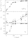 |
Fig. 12 Parameters of the best fits to the continuum spectra, as a function of time from the onset of the radio outburst (July 10, 2016). The plotted parameter is indicated in the bottom right of each panel. |
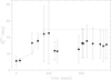 |
Fig. 13 Lower limit on the opening angle estimated from Eq. (10) for all the epochs of our monitoring. The bars indicate the standard deviation of the values obtained in the different bands. The dashed line connects the values of θ0 obtained from the best fits to the spectra (see Table 6). |
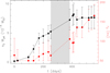 |
Fig. 14 Ionised jet mass (solid black curve) and inner radius (dashed red curve) as a function of time from the onset of the radio outburst (July 10, 2016). The grey area separates the period when the jet is still powered by the outburst from that when the feeding mechanism is quenched. |
5 Summary and conclusions
As a follow-up to Paper I, we monitored the radio continuum emission of the outburst from the massive YSO S255IR NIRS 3 over ~13 months at six wavelengths with the VLA. We also imaged the radio jet at 3 mm with ALMA at two epochs separated by ~27 months, with an angular resolution ≲0″.1. Our results indicate that after an exponential increase in the radio flux in all observed bands, the intensity becomes constant or slightly decreasing. A comparison of the two ALMA maps shows that the radio jet is expanding both to the NE and SW, although only the NE lobe was present during our VLA monitoring. The SW lobe appeared between May 2018 and June 2019, namely at a much later time than the NE lobe. We believe that this ejection event is related to the same accretion outburst, which occurred in 2015. We speculate that the delay between the two lobes might be due to a greater density of the medium facing the SW lobe, which could curb the expansion of the jet on that side.
From the analysis of the continuum spectra, we infer that two mechanisms are needed to explain the observed fluxes: free-free emission at short wavelengths and non-thermal (probably synchrotron) emission at long wavelengths. We believe that the latter should become dominant at frequencies ≲6 GHz. For this reason, we fitted only the data with v ≥ 6 GHz using a slightly modified version of the jet model adopted in Paper I, which works for any opening angle of the jet <90º. We conclude that the spectra can be satisfactorily reproduced with an expanding, decelerating, mono-polar thermal jet that was actively powered by the outburst until mid-2017. After this date, no more mass is injected into the lobes and the inner jet radius expands, which, over the long term, is bound to give rise to one of the knots that characterise thermal jets from YSOs.
Acknowledgements
A.C.G. acknowledges from PRIN-MUR 2022 20228JPA3A “The path to star and planet formation in the JWST era (PATH)” and by INAF-GoG 2022 “NIR-dark Accretion Outbursts in Massive Young stellar objects (NAOMY)” and Large Grant INAF 2022 “YSOs Outflows, Disks and Accretion: towards a global framework for the evolution of planet forming systems (YODA)”. R.F. acknowledges support from the grants Juan de la Cierva JC2021-046802-I, PID2020-114461GB-I00 and CEX2021-001131-S funded by MCIN/AEI/ 10.13039/501100011033 and by “European Union NextGenera-tionEU PRTR”. T.P.R. acknowledges support from ERC grant 743029 EASY. This study is based on observations made under project 16A-424, 16B-427, and 17B-045 of the VLA of NRAO. The National Radio Astronomy Observatory is a facility of the National Science Foundation operated under cooperative agreement by Associated Universities, Inc.. This paper makes also use of the following ALMA data: ADS/JAO.ALMA#2018.1.00864.S. ALMA is a partnership of ESO (representing its member states), NSF (USA) and NINS (Japan), together with NRC (Canada), NSC and ASIAA (Taiwan), and KASI (Republic of Korea), in cooperation with the Republic of Chile. The Joint ALMA Observatory is operated by ESO, AUI/NRAO and NAOJ.
Appendix A Jet expansion law
As discussed in Sect. 4.3.1, the jet is not expanding at constant velocity during the period of our monitoring, but it appears to slow down. It is thus necessary to adopt an expression for the maximum radius, rm, that properly takes this effect into account. A reasonable scenario may be that of a jet confined in a solid angle Ω, with initial mass M0, which expands with initial velocity υ0 through a medium with density ρ ∝ r−2, where r is the distance from the jet origin. Because of momentum conservation one can write
![Mathematical equation: $\eqalign{ & {M_0}{v_0} = M(t){{{\rm{d}}{r_{\rm{m}}}} \over {{\rm{d}}t}} \cr & \,\,\,\,\,\,\,\,\,\,\,\,\, = \left[ {{M_0} + \int_{{r_{{\rm{m}}0}}}^{{r_{\rm{m}}}} {{\rho _0}} {{\left( {{{{r_{{\rm{m}}0}}} \over r}} \right)}^2}{\rm{\Omega }}{r^2}{\rm{d}}r} \right]{{{\rm{d}}{r_{\rm{m}}}} \over {{\rm{d}}t}} \cr & \,\,\,\,\,\,\,\,\,\,\,\,\, = \left[ {{M_0} + {\rm{\Omega }}{\rho _0}r_{{\rm{m}}0}^2\left( {{r_{\rm{m}}} - {r_{{\rm{m}}0}}} \right)} \right]{{{\rm{d}}{r_{\rm{m}}}} \over {{\rm{d}}t}}, \cr} $](/articles/aa/full_html/2023/12/aa47468-23/aa47468-23-eq68.png) (A.1)
(A.1)
with ρ0 density at radius rm0. The solution of this differential equation is
![Mathematical equation: $\eqalign{ & {M_0}{v_0}t = {M_0}\left( {{r_{\rm{m}}} - {r_{{\rm{m}}0}}} \right) \cr & \,\,\,\,\,\,\,\,\,\,\,\,\,\,\,\,\,\, + {\rm{\Omega }}{\rho _0}r_{{\rm{m}}0}^2\left[ {{{r_{\rm{m}}^2 - r_{{\rm{m}}0}^2} \over 2} - {r_{{\rm{m}}0}}\left( {{r_{\rm{m}}} - {r_{{\rm{m}}0}}} \right)} \right], \cr} $](/articles/aa/full_html/2023/12/aa47468-23/aa47468-23-eq69.png) (A.2)
(A.2)
which after some algebra gives
 (A.3)
(A.3)
where we have defined  .
.
While this expression provides us with a more realistic description of the jet expansion than the constant velocity assumption adopted in Paper I, we stress that it is not to be taken as the real equation of motion of the jet but as the simplest way to parametrise the observed deceleration of it.
Appendix B Description of the model
In Paper I we adopted the jet model by Reynolds (1986) to describe the integrated flux density of the radio jet from S255IR NIRS 3. More specifically, we assumed what is defined as the ‘standard spherical’ case in Reynolds’ Table 1, namely a jet where the opening angle (θ0), internal velocity (υ0), ionisation degree (x0), and temperature (T0) do not depend on the distance r from the star. Conservation of mass along the flow implies that the gas number density can be expressed as n = n0(r/r0)−2.
Despite its simplicity, the model was successful in fitting the observed spectra in Paper I. However, Reynolds’ equations have been derived under the assumptions of small θ0, an approximation that is not satisfied by the best fit to the radio spectra obtained in Paper I (see Table 3 there), which requires angles as large as ~50º. In order to overcome this limitation, we propose here a slightly modified version of Reynolds’ model that works for any θ0 < 9oº.
To allow for an analytic solution of the equations, we maintain Reynolds’ assumption that the opacity depends only on r. This is equivalent to assuming that the jet is not conical but has a pyramidal shape with two faces parallel to the line of sight. We also assumed that the jet is delimited by two cylindrical surfaces, with radii r0 and rm, and that its axis is inclined by a small angle, ψ, with respect to the plane of the sky. Figure B.1 schematically illustrates the geometry of the jet, where the star lies at the origin of the axes and the line of sight is parallel to the ɀ-axis.
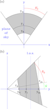 |
Fig. B.1 Sketch of the jet model. The x- and y-axes lie in the plane of the sky, and the ɀ-axis is parallel to the line of sight. The y-axis coincides with the projection of the jet axis on the plane of the sky. The dotted line labelled ‘l.o.s.’ denotes a generic line of sight. The star powering the jet lies at the origin of the coordinate system. |
Following Reynolds, the absorption coefficient of the ionised gas and the opacity can be written as
 (B.1)
(B.1)
where
 (B.2)
(B.2)
with aĸ = 0.212 in CGS units, and
![Mathematical equation: $\eqalign{ & \tau (R) = \int_{ - R\tan \left( {{\theta _0} - \psi } \right)}^{R\tan \left( {{\theta _0} + \psi } \right)} \kappa {\rm{d}}z = {\kappa _0}r_0^4\int_{ - R\tan \left( {{\theta _0} - \psi } \right)}^{R\tan \left( {{\theta _0} + \psi } \right)} {{{\left( {{R^2} + {z^2}} \right)}^{ - 2}}} {\rm{d}}z \cr & \,\,\,\,\,\,\,\,\,\,\, = {{{\kappa _0}r_0^4} \over {2{R^3}}}\left[ {{{\tan \left( {{\theta _0} + \psi } \right)} \over {1 + {{\tan }^2}\left( {{\theta _0} + \psi } \right)}} + {{\tan \left( {{\theta _0} - \psi } \right)} \over {1 + {{\tan }^2}\left( {{\theta _0} - \psi } \right)}} + 2{\theta _0}} \right] \cr & \,\,\,\,\,\,\,\,\,\, = {{{\kappa _0}r_0^4} \over {2{R^3}}}\left[ {\sin \left( {2{\theta _0}} \right)\cos (2\psi ) + 2{\theta _0}} \right] \cr & \,\,\,\,\,\,\,\,\,\, = {\tau _0}{\left( {{{{r_0}} \over R}} \right)^3}. \cr} $](/articles/aa/full_html/2023/12/aa47468-23/aa47468-23-eq74.png) (B.3)
(B.3)
Here we have defined the two quantities
 (B.4)
(B.4)
and
 (B.5)
(B.5)
To ease the comparison with Reynolds’ expressions, we indicate with y0 and ym the projections of r0 and rm on the plane of the sky, namely y0 = r0 cos ψ and ym = rm cos ψ, and with y1 the value of R at which τ(R) = 1. From Eq. (B.3) one has
 (B.6)
(B.6)
For the calculation of the total flux density of the jet we follow Reynolds’ approach and assume that the emission between R = 0 and R = y1 is optically thick, and that between R = y1 and R = ym is optically thin. Under this approximation the flux can be written as
![Mathematical equation: $\eqalign{ & {S_v} = {1 \over {{d^2}}}\int_{{y_0}}^{{y_{\rm{m}}}} {{B_v}} \left( {{T_0}} \right)\left( {1 - {{\rm{e}}^{ - \tau }}} \right)2{{\theta '}_0}R{\rm{d}}R \cr & \,\,\,\,\,\,\, \simeq {{2{{\theta '}_0}{B_v}\left( {{T_0}} \right)} \over {{d^2}}}\left[ {\int_{{y_0}}^{{y_1}} R {\rm{d}}R + \int_{{y_1}}^{{y_{\rm{m}}}} \tau (R)R{\rm{d}}R} \right] \cr & \,\,\,\,\,\,\, = {{2{{\theta '}_0}{B_v}\left( {{T_0}} \right)} \over {{d^2}}}\left[ {{{y_1^2 - y_0^2} \over 2} + y_1^3\left( {{1 \over {{y_1}}} - {1 \over {{y_{\rm{m}}}}}} \right)} \right], \cr} $](/articles/aa/full_html/2023/12/aa47468-23/aa47468-23-eq78.png) (B.7)
(B.7)
where Bv is the Planck function and θ′0 is the projection of θ0 on the plane of the sky. The two angles are related by the expression
 (B.8)
(B.8)
We note that it is not strictly correct to integrate from y0 to ym because the projections of the two circles with radii r0 and rm on the plane of the sky are ellipses, and the integral should be made not only in the variable R but also in the azimuthal angle. However, the approximation adopted by us is acceptable for small ψ.
The expression of Sv in the case of a jet totally thin (y1 < y0) or thick (y1 > ym) can be obtained in a similar way, by considering only the relevant approximation in the argument of the integral in Eq. (B.7). In conclusion, one obtains
![Mathematical equation: $\eqalign{ & {S_v} = {{2{{\theta '}_0}{B_v}\left( {{T_0}} \right)} \over {{d^2}}} \cr & \,\,\,\,\,\,\,\,\,\,\, \times \left\{ {\matrix{ {y_1^3\left( {{1 \over {{y_0}}} - {1 \over {{y_{\rm{m}}}}}} \right)} \hfill & { \Leftrightarrow {y_1} \le {y_0}} \hfill \cr {\left[ {{{y_1^2 - y_0^2} \over 2} + y_1^3\left( {{1 \over {{y_1}}} - {1 \over {{y_{\rm{m}}}}}} \right)} \right]} \hfill & { \Leftrightarrow {y_0} < {y_1} < {y_{\rm{m}}}.} \hfill \cr {{{y_{\rm{m}}^2 - y_0^2} \over 2}} \hfill & { \Leftrightarrow {y_1} \ge {y_{\rm{m}}}} \hfill \cr } } \right. \cr} $](/articles/aa/full_html/2023/12/aa47468-23/aa47468-23-eq80.png) (B.9)
(B.9)
We note that this expression gives the total flux emitted by a single jet lobe, whereas Eq. (5) of Paper I takes into account both lobes. The different approach is justified by the fact that our new findings have proved that only the NE lobe was present during our monitoring (see Sect. 4.1).
The quantity y1 is a function of n0, in addition to other parameters. However, following Reynolds, it may be convenient to express it in terms of the mass loss rate of the jet,  , which is obtained by integrating the flux of mass through the inner surface of the jet. Obviously,
  does not depend on the inclination of the jet with respect to the line of sight, so we can simplify the calculation by assuming ψ = 0. Hence, we obtain
 (B.10)
where µ is the mean particle mass per hydrogen atom (we assume µ = 1.67 × 10⁻²⁴ g) and  is the component of the velocity perpendicular to the inner surface of the jet. From this it is trivial to express n0 as a function of
  , and from Eqs. (B.2), (B.5), and (B.6) one obtains
 (B.11)
where we have defined  .
.
Finally, a quantity of interest for our purposes is the ionised mass of the jet, which is given by the expression
 (B.12)
 (B.13)
where we have used Eq. (B.10) to replace n0.
References
- Audard, M., Ábrahám, P., Dunham, M. M., et al. 2014, in Protostars and Planets VI, eds. T. Henning, C. P. Dullemond, R. S. Klessen, & H. Beuther (Tucson: University of Arizona Press), 387 [Google Scholar]
- Beltrán, M. T., & de Wit, W. J. 2016, A&ARv, 24, 6 [Google Scholar]
- Beltrán, M. T., Cesaroni, R., Moscadelli, L., et al. 2016, A&A, 593, A49 [NASA ADS] [CrossRef] [EDP Sciences] [Google Scholar]
- Boley, P.A., Linz, H., van Boekel, R., et al. 2013, A&A, 558, A24 [NASA ADS] [CrossRef] [EDP Sciences] [Google Scholar]
- Brogan, C. L., Hunter, T. R., Cyganowski, C. J., et al. 2018, ApJ, 866, 87 [NASA ADS] [CrossRef] [Google Scholar]
- Burns, R. A., Handa, T., Nagayama, T., Sunada, K., & Omodaka, T. 2016, MNRAS, 460, 283 [NASA ADS] [CrossRef] [Google Scholar]
- Burns, R. A., Sugyiama, K., Hirota, T., et al. 2020, Nat. Astron., 4, 506 [NASA ADS] [CrossRef] [Google Scholar]
- Burns, R. A., Uno, Y., Sakai, N., et al. 2023, Nat. Astron., 7, 557 [CrossRef] [Google Scholar]
- Caratti o Garatti, A., Stecklum, B., Garcia Lopez, R., et al. 2017, Nat. Phys., 13, 276 [Google Scholar]
- Carraco-González, C., Rodríguez, L.F., Anglada, G. et al. 2010, Science, 330, 1209 [CrossRef] [Google Scholar]
- Cesaroni, R., Neri, R., Olmi, L., et al. 2005, A&A, 434, 1039 [NASA ADS] [CrossRef] [EDP Sciences] [Google Scholar]
- Cesaroni, R., Moscadelli, L., Neri, R., et al. 2018, A&A, 612, A103 (Paper I) [NASA ADS] [CrossRef] [EDP Sciences] [Google Scholar]
- Chen, Z., Sun, W., Chini, R., et al. 2021, ApJ, 922, 90 [NASA ADS] [CrossRef] [Google Scholar]
- D’Alessio, P., Calvet, N., & Hartmann, L. 2001, ApJ, 553, 321 [Google Scholar]
- de Oña Wilhelmi, E., López-Coto, R., & Su, Y. 2023, MNRAS, 523, 105 [CrossRef] [Google Scholar]
- Fedriani, R., Caratti o Garatti, A., Purser, S. J. D., et al. 2019, Nat. Commun., 10, 3630 [NASA ADS] [CrossRef] [Google Scholar]
- Fedriani, R., Caratti o Garatti, A., Cesaroni, R., et al. 2023, A&A, 676, A107 [NASA ADS] [CrossRef] [EDP Sciences] [Google Scholar]
- Fischer, W. J., Hillenbrand, L. A., Herczeg, G. J., et al. 2023, in Protostars and Planets VII, eds. S. Inutsuka, Y. Aikawa, T. Muto, K. Tomida, & M. Tamura (San Francisco, CA: Astronomical Society of the Pacific), 355 [Google Scholar]
- Fujisawa, K., Yonekura, Y., Sugiyama, K., et al. 2015, ATel, 8286, 1 [NASA ADS] [Google Scholar]
- Goddi, C., Moscadelli, L., Sanna, A., Cesaroni, R., & Minier, V. 2007, A&A, 461, 1027 [NASA ADS] [CrossRef] [EDP Sciences] [Google Scholar]
- Hirota, T., Cesaroni, R., Moscadelli, L., et al. 2021, A&A, 647, A23 [NASA ADS] [CrossRef] [EDP Sciences] [Google Scholar]
- Hunter, T. R., Brogan, C. L., MacLeod, G., et al. 2017, ApJ, 837, L29 [NASA ADS] [CrossRef] [Google Scholar]
- Hunter, T. R., Brogan, C. L., De Buizer, J. M., et al. 2021, ApJ, 912, L17 [CrossRef] [Google Scholar]
- Lampton, M., Margon, B., & Bowyer, S. 1976, ApJ, 208, 177 [Google Scholar]
- Liu, S.-Y., Su, Y.-N., Zinchenko, I., Wang, K.-S., Wang, Y. 2018, ApJ, 863, L12 [NASA ADS] [CrossRef] [Google Scholar]
- Liu, S.-Y., Su, Y.-N., Zinchenko, I., et al. 2020, ApJ, 904, 181 [Google Scholar]
- Moscadelli, L., Cesaroni, R., Sánchez-Monge, Á., et al. 2013, A&A, 558, A145 [NASA ADS] [CrossRef] [EDP Sciences] [Google Scholar]
- Moscadelli, L., Sanna, A., Goddi, C., et al. 2017, A&A, 600, A8 [Google Scholar]
- Obonyo, W. O., Lumsden, S. L., Hoare, M. G., Kurtz, S. E., & Purser, S. J. D. 2021, MNRAS, 501, 5197 [NASA ADS] [CrossRef] [Google Scholar]
- Reynolds, S.P. 1986, ApJ, 304, 713 [NASA ADS] [CrossRef] [Google Scholar]
- Sadavoy, S. I., Di Francesco, J., Johnstone, D., et al. 2013, ApJ, 767, 126 [Google Scholar]
- Sánchez-Monge, Á., Beltrán, M. T., Cesaroni, R., et al. 2014, A&A, 569, A11 [NASA ADS] [CrossRef] [EDP Sciences] [Google Scholar]
- Sánchez-Monge, Á., Schilke, P., Ginzburg, A., Cesaroni, R., & Schmiedeke, A. 2018, A&A, 609, A101 [NASA ADS] [CrossRef] [EDP Sciences] [Google Scholar]
- Sanna, A., Moscadelli, L., Goddi, C., et al. 2019, A&A, 623, A3 [NASA ADS] [CrossRef] [EDP Sciences] [Google Scholar]
- Shepherd, D.S., Yu, K.C., Bally, J., & Testi, L. 2000, ApJ, 535, 833 [NASA ADS] [CrossRef] [Google Scholar]
- Staff, J. E., Tanaka, K. E. I., & Tan, J. C. 2019, ApJ 882, 123 [Google Scholar]
- Stecklum, B., Caratti o Garatti, A., Cardenas, M. C., et al. 2016, ATel, 8732, 1 [NASA ADS] [Google Scholar]
- Stecklum, B., Wolf V., Linz H., et al. 2021, A&A, 646, A161 [NASA ADS] [CrossRef] [EDP Sciences] [Google Scholar]
- Testi, L., Birnstiel, T., Ricci, L., et al. 2014, in Protostars and Planets VI, eds. T. Henning, C. P. Dullemond, R. S. Klessen, & H. Beuther (Tucson: Univ. of Arizona Press), 339 [Google Scholar]
- Uchiyama, M., Yamashita, T., Sugyiama, K., et al. 2020, PASJ, 72, 4 [NASA ADS] [CrossRef] [Google Scholar]
- Wang, Y., Beuther, H., Bik, A., et al. 2011, A&A, 527, A32 [NASA ADS] [CrossRef] [EDP Sciences] [Google Scholar]
- Zinchenko, I., Liu, S.-Y., Su, Y.-N., et al. 2015, ApJ, 810, 10 [NASA ADS] [CrossRef] [Google Scholar]
The Common Astronomy Software Applications software can be downloaded at http://casa.nrao.edu
Available at http://vlbi.sci.ibaraki.ac.jp/iMet/data/192.6-00
The M2O is a global cooperative of maser monitoring programmes; see https://masermonitoring.org
We stress that our definition of θ0 corresponds to one-half of the θ0 defined by Reynolds (1986).
All Tables
Typical 1σ RMS noise and synthesised beam for different bands and VLA configurations.
Flux densities in millijanskys measured at 92.5 GHz with ALMA towards the NE and SW components of S255IR NIRS 3.
All Figures
|
Fig. 1 Maps of the 3 mm continuum emission obtained with ALMA. (a) Data acquired on June 6, 2019. Contour levels range from 0.52 to 16.12 in steps of 2.6 mJy beam−1. The cross marks the peak of the 900 μm continuum emission imaged by Liu et al. (2020). The circle in the bottom left represents the synthesised beam. (b) Same as the top panel, but for the map obtained on September 3, 2021. Contour levels range from 0.29 to 16.24 in steps of 1.45 mJy beam−1. |
| In the text | |
|
Fig. 2 Maps of the line emission obtained with ALMA. (a) Map of the emission averaged over the H13CN(1−0) line (white contours) overlaid on the continuum image at 3 mm obtained on June 6, 2019. Contour levels range from 1.2 to 4.56 in steps of 0.48 mJy beam−1. The circle in the bottom left represents the synthesised beam. (b) Same as the top panel, but for the SO(22−11) line. Contour levels range from 1.65 to 4.62 in steps of 0.33 mJy beam−1. |
| In the text | |
|
Fig. 3 Maps of the 3.6 cm continuum emission obtained with the VLA on July 10, 2016 (red) and of the 3 mm continuum emission (blue), also shown in Fig. 1b. The dashed lines denote the symmetry axes of the bipolar structures. Red contour levels range from 0.1 to 0.6 in steps of 0.1 mJy beam−1. Blue contour levels range from 0.29 to 8.99 in steps of 2.9 mJy beam−1. |
| In the text | |
|
Fig. 4 Continuum spectra of the variable, compact component in S255IR NIRS 3. The date of the observations is given in the top left of each panel. The vertical error bars assume a calibration error of 10% in all bands, while the horizontal bars indicate the bandwidth covered at each frequency. The upper limits denote that the flux density is also contributed by the emission from the large-scale lobes, due to the limited angular resolution. Red symbols mark data in the L (1.5 GHz) and S (3 GHz) bands. The curves are the best fits obtained with the model of a thermal jet described in Sect. 4.3.2. |
| In the text | |
|
Fig. 5 Distribution of the peaks of the 3 mm and 1.3 cm continuum maps obtained, respectively, with ALMA and with the A and B configurations of the VLA. The circles indicate our VLA data, the triangle the data of OLHKP, and the two squares our ALMA data. The dashed line connects the points in order of time (the first point in the bottom-right corner corresponds to the observation on July 10, 2016). The third point from the top left is obtained from the OLHKP data. The cross marks the position of the (proto)star, and the solid red line is the axis of the radio jet (PA = 48°). The dotted ellipses are the synthesised beams scaled down by a factor of 5. |
| In the text | |
|
Fig. 6 Flux density of the variable, compact source in S255IR NIRS 3 as a function of time from the beginning of the radio burst (July 10, 2016) in all bands observed with the VLA. The two rightmost points are the measurements at 6 and 22 GHz by OLHKP. Curves are colour-coded by frequency (in gigahertz). Arrows denote points with upper limits (see Sect. 2.1), which are connected by dashed lines. The two black arrows pointing to the right indicate the flux densities at 92 GHz of the NE lobe (see Table 1) measured 1061 and 1881 days after the radio burst. Typical error bars are shown in the bottom right of the figure. The vertical dotted lines mark the beginning and end of an array configuration, as labelled above the figure. |
| In the text | |
|
Fig. 7 Maps of the 3 mm continuum emission (contours) overlaid on the corresponding map of the spectral index at 3 mm. (a) Data obtained with ALMA on June 6, 2019. Black contour levels range from 10% to 90% in steps of 10% of the peak emission. White contour levels correspond to a spectral index equal to 0. The cross marks the position of the (proto)star. The circle in the bottom left represents the synthesised beam. (b) Same as the top panel, but for the map obtained on September 3, 2021. |
| In the text | |
|
Fig. 8 Map of the 3 mm continuum emission obtained with ALMA on September 3, 2021, overlaid on the 1.3 cm image obtained by OLHKP on May 5, 2018. Contour levels are the same as in Fig. 1b. The cross marks the position of the (proto)star. The ellipse in the bottom left represents the synthesised beam at 1.3 cm. |
| In the text | |
|
Fig. 9 Water masers spots (solid circles) observed by Goddi et al. (2007; cyan), Burns et al. (2016; green), and Hirota et al. (2021; magenta) overlaid on the 3 mm continuum map (blue contours) of Fig. 1b. The dashed lines indicate the jet axes in the two tracers. The cross marks the position of the (proto)star. The circle in the bottom left represents the synthesised beam at 3 mm. |
| In the text | |
|
Fig. 10 Comparison between the observed maps of the NE lobe of the radio jet (left panels) with the best-fit maps obtained with the model (right panels). The top panels correspond to the first ALMA epoch, bottom panels to the second one. The horizontal axis is parallel to the jet axis. Contour levels range from 10% to 90% in steps of 10% of the peak of each image. The circle in the bottom left represents the synthesised beam. |
| In the text | |
|
Fig. 11 Comparison of the projection on the plane of the sky of the outer radius of the jet, ym (blue), with the position of the brightness temperature peak, ypeak (black), and the border between the optically thin and optically thick parts of the jet, y1 (red). All quantities are plotted as a function of time from the onset of the radio outburst (July 10, 2016). The black circles indicate our VLA data, the triangle the OLHKP data, and the two squares our ALMA data. We remark that ypeak is measured from Fig. 5 as the separation between the star and the projection of the peak along the jet axis. |
| In the text | |
|
Fig. 12 Parameters of the best fits to the continuum spectra, as a function of time from the onset of the radio outburst (July 10, 2016). The plotted parameter is indicated in the bottom right of each panel. |
| In the text | |
|
Fig. 13 Lower limit on the opening angle estimated from Eq. (10) for all the epochs of our monitoring. The bars indicate the standard deviation of the values obtained in the different bands. The dashed line connects the values of θ0 obtained from the best fits to the spectra (see Table 6). |
| In the text | |
|
Fig. 14 Ionised jet mass (solid black curve) and inner radius (dashed red curve) as a function of time from the onset of the radio outburst (July 10, 2016). The grey area separates the period when the jet is still powered by the outburst from that when the feeding mechanism is quenched. |
| In the text | |
|
Fig. B.1 Sketch of the jet model. The x- and y-axes lie in the plane of the sky, and the ɀ-axis is parallel to the line of sight. The y-axis coincides with the projection of the jet axis on the plane of the sky. The dotted line labelled ‘l.o.s.’ denotes a generic line of sight. The star powering the jet lies at the origin of the coordinate system. |
| In the text | |
Current usage metrics show cumulative count of Article Views (full-text article views including HTML views, PDF and ePub downloads, according to the available data) and Abstracts Views on Vision4Press platform.
Data correspond to usage on the plateform after 2015. The current usage metrics is available 48-96 hours after online publication and is updated daily on week days.
Initial download of the metrics may take a while.