| Issue |
A&A
Volume 692, December 2024
|
|
|---|---|---|
| Article Number | A181 | |
| Number of page(s) | 8 | |
| Section | Interstellar and circumstellar matter | |
| DOI | https://doi.org/10.1051/0004-6361/202452458 | |
| Published online | 12 December 2024 | |
Fine structure and kinematics of the ionized and molecular gas in the jet and disk around S255IR NIRS3 from high-resolution ALMA observations
1
Federal Research Center A.V. Gaponov-Grekhov Institute of Applied Physics of the Russian Academy of Sciences,
46 Ul’yanov str.,
Nizhny Novgorod
603950,
Russia
2
Institute of Astronomy and Astrophysics, Academia Sinica,
11F of ASMAB, AS/NTU No.1, Sec. 4, Roosevelt Rd,
Taipei
10617,
Taiwan
Received:
1
October
2024
Accepted:
31
October
2024
Abstract
Aims. We present observations of the high-mass star-forming region S255IR, which harbors the ~20 M⊙ protostar NIRS3, where a disk-mediated accretion burst was recorded several years ago. The angular resolution of these observations, of ~15 mas, corresponds to ~25 au, which is almost an order of magnitude better than in the previous studies of this object.
Methods. The observations were performed with the Atacama Large Millimeter/submillimeter Array (ALMA) at a wavelength of 0.9 mm in continuum and in several molecular lines.
Results. In the continuum, we detect the central bright source (brightness temperature of ~850 K) elongated along the jet direction and two pairs of bright knots in the jet lobes. These pairs of knots imply a double ejection from NIRS3 with a time interval of ~1.5 years. The orientation of the jet differs by ~20° from that on larger scales, as also mentioned in some other recent works. The 0.9 mm continuum emission of the central source represents a mixture of the dust thermal emission and free-free emission of the ionized gas. Certain properties of the free-free emission are typical of hypercompact H II regions. In the continuum emission of the knots in the jet, the free-free component apparently dominates. In the molecular lines, a sub-Keplerian disk is observed around NIRS3 of about 400 au in diameter. The absorption features in the molecular lines toward the central bright source may indicate an infall. The molecular line emission appears highly inhomogeneous at small scales, which may indicate a small-scale clumpiness in the disk.
Key words: stars: formation / stars: massive / ISM: clouds / ISM: molecules / submillimeter: ISM / ISM: individual objects: S255IR
© The Authors 2024
 Open Access article, published by EDP Sciences, under the terms of the Creative Commons Attribution License (https://creativecommons.org/licenses/by/4.0), which permits unrestricted use, distribution, and reproduction in any medium, provided the original work is properly cited.
This article is published in open access under the Subscribe to Open model. This email address is being protected from spambots. You need JavaScript enabled to view it. to support open access publication.
1 Introduction
There are still several competing scenarios explaining high-mass star formation (e.g., Tan et al. 2014; Motte et al. 2018; Rosen et al. 2020; Padoan et al. 2020). In recent years, significant attention has been paid to the luminosity outbursts in massive protostars, which are believed to be caused by episodic disk-mediated accretion events. There are theoretical models that predict this kind of behavior (e.g., Meyer et al. 2017, 2019). To date, several such bursts have been recorded (Caratti O Garatti et al. 2017; Brogan et al. 2019; Proven-Adzri et al. 2019; Hunter et al. 2017; Tapia et al. 2013; Chen et al. 2021; Wolf et al. 2024). One of the first was the burst in S255IR NIRS3, which was observed at IR (Caratti O Garatti et al. 2017) and submillimeter (Liu et al. 2018) wavelengths, and was accompanied by the methanol maser flare (Moscadelli et al. 2017; Szymczak et al. 2018).
S255IR, at a distance of ![Mathematical equation: $\[1.78_{-0.11}^{+0.12}\]$](/articles/aa/full_html/2024/12/aa52458-24/aa52458-24-eq1.png) kpc (Burns et al. 2016), is a well-known site of high-mass star formation (e.g., Zinchenko et al. 2024), and is part of the large star-forming complex sandwiched between the evolved H II regions S255 and S257 (Ojha et al. 2011). It contains three major cores SMA1, SMA2, and SMA3 (Wang et al. 2011) and several smaller condensations (Zinchenko et al. 2020). The SMA1 core harbors a ~20 M⊙ protostar NIRS3 (Zinchenko et al. 2015), the mass of which is estimated from the bolometric luminosity of ~3 × 10⁴ L⊙ at the adopted distance.
kpc (Burns et al. 2016), is a well-known site of high-mass star formation (e.g., Zinchenko et al. 2024), and is part of the large star-forming complex sandwiched between the evolved H II regions S255 and S257 (Ojha et al. 2011). It contains three major cores SMA1, SMA2, and SMA3 (Wang et al. 2011) and several smaller condensations (Zinchenko et al. 2020). The SMA1 core harbors a ~20 M⊙ protostar NIRS3 (Zinchenko et al. 2015), the mass of which is estimated from the bolometric luminosity of ~3 × 10⁴ L⊙ at the adopted distance.
A disk-outflow system is associated with this protostar (Zinchenko et al. 2015). Assuming Keplerian rotation, Zinchenko et al. (2015) derived an inclination angle for the disk of ~25° based on SubMillimeter Array (SMA) data. However, the IR image implies the disk is seen almost edge-on (Boley et al. 2013). An analysis of the ALMA (Atacama Large Millimeter/submillimeter Array) data with a much higher angular resolution of ![Mathematical equation: $\[\sim 0^{\prime\prime}_\cdot 14\]$](/articles/aa/full_html/2024/12/aa52458-24/aa52458-24-eq2.png) led to the conclusion that the observed rotating structure represents an infalling envelope or pseudo-disk in sub-Keplerian rotation (Liu et al. 2020). Liu et al. (2020) assumed an upper limit for the radius of the probable centrifugal barrier at ~125 AU.
led to the conclusion that the observed rotating structure represents an infalling envelope or pseudo-disk in sub-Keplerian rotation (Liu et al. 2020). Liu et al. (2020) assumed an upper limit for the radius of the probable centrifugal barrier at ~125 AU.
The IR jet in this area was detected many years ago (Howard et al. 1997). Recently, detailed multi-frequency (up to ~92 GHz) studies of the radio jets were performed with a maximum angular resolution of ![Mathematical equation: $\[\sim 0^{\prime\prime}_\cdot 1\]$](/articles/aa/full_html/2024/12/aa52458-24/aa52458-24-eq3.png) (Obonyo et al. 2021; Cesaroni et al. 2023, 2024). Here, we report and discuss new ALMA observations of this object with an angular resolution that is almost an order of magnitude higher than in previous studies.
(Obonyo et al. 2021; Cesaroni et al. 2023, 2024). Here, we report and discuss new ALMA observations of this object with an angular resolution that is almost an order of magnitude higher than in previous studies.
2 Observations
We carried out our observations with the ALMA toward S255IR SMA1 under the project #2019.1.00315.S, obtaining an image of the continuum emission with a maximum angular resolution of ![Mathematical equation: $\[\sim 0^{\prime\prime}_\cdot 015\]$](/articles/aa/full_html/2024/12/aa52458-24/aa52458-24-eq4.png) (~27 au). One observation was carried out on 2021 September 3 with a hybrid C43-9/10 configuration with 45 antennas in the 12 m array. The on-source integration time of the C43-9/10 observation is about 18.5 min, and the baseline lengths range from 121 m to 16.2 km. The phase center in the ICRS reference frame was Right Ascension
(~27 au). One observation was carried out on 2021 September 3 with a hybrid C43-9/10 configuration with 45 antennas in the 12 m array. The on-source integration time of the C43-9/10 observation is about 18.5 min, and the baseline lengths range from 121 m to 16.2 km. The phase center in the ICRS reference frame was Right Ascension ![Mathematical equation: $\[(\mathrm{RA})=06^{\mathrm{h}} 12^{\mathrm{h}} 54^\text{s}_\cdot013\]$](/articles/aa/full_html/2024/12/aa52458-24/aa52458-24-eq5.png) (J2000) and Declination
(J2000) and Declination ![Mathematical equation: $\[(\text{Dec}) = +17^{\circ} 59^{\prime} 23^{\prime \prime}_\cdot 050\]$](/articles/aa/full_html/2024/12/aa52458-24/aa52458-24-eq6.png) . To maximize the aggregated bandwidth for the continuum maps, the ALMA correlator was configured to provide four 1.875 GHz spectral windows centered at 334.593, 336.583, 346.593, and 348.593 GHz with a spectral resolution of 1.13 MHz (~1.0 km s−1) after the online Hanning-smooth. Molecular line transitions, such as C34S, SiO (8–7), CO (3–2), and CH3CN (19–18), are simultaneously captured by the designed spectral windows. The half-power width of the ALMA 12 m primary beam was ~17.04″ at 341.5 GHz, which is more than sufficient to cover the entire extent of the S255IR SMA1. The quasar J0510+1800 was observed to calibrate passband and absolute flux scale. The quasar J0613+1708 was observed as the gain calibrator. The acquired visibility data were reduced using the observatory pipeline in CASA (Common Astronomy Software Application) version 6.2.1.7. The synthesized beam of the continuum map was ~19 × 13 mas, which corresponds to ~34×23 AU at the distance of S255IR. The synthesized beams for the spectral line maps are almost the same.
. To maximize the aggregated bandwidth for the continuum maps, the ALMA correlator was configured to provide four 1.875 GHz spectral windows centered at 334.593, 336.583, 346.593, and 348.593 GHz with a spectral resolution of 1.13 MHz (~1.0 km s−1) after the online Hanning-smooth. Molecular line transitions, such as C34S, SiO (8–7), CO (3–2), and CH3CN (19–18), are simultaneously captured by the designed spectral windows. The half-power width of the ALMA 12 m primary beam was ~17.04″ at 341.5 GHz, which is more than sufficient to cover the entire extent of the S255IR SMA1. The quasar J0510+1800 was observed to calibrate passband and absolute flux scale. The quasar J0613+1708 was observed as the gain calibrator. The acquired visibility data were reduced using the observatory pipeline in CASA (Common Astronomy Software Application) version 6.2.1.7. The synthesized beam of the continuum map was ~19 × 13 mas, which corresponds to ~34×23 AU at the distance of S255IR. The synthesized beams for the spectral line maps are almost the same.
Under the project #2019.1.00315.S, we also carried out band 7 observations at ![Mathematical equation: $\[\sim 0^{\prime\prime}_\cdot 1\]$](/articles/aa/full_html/2024/12/aa52458-24/aa52458-24-eq7.png) in order to monitor the temporal variation of S255IR SMA1 in dust continuum and molecular line emission. Two executions were carried out on 2021 June 13 and July 6 with antennas 41 and 40 in the 12 m array, respectively. The total on-source integration time is about 90 min. The synthesized beam was ~0.109 × 0.975 arcsec.
in order to monitor the temporal variation of S255IR SMA1 in dust continuum and molecular line emission. Two executions were carried out on 2021 June 13 and July 6 with antennas 41 and 40 in the 12 m array, respectively. The total on-source integration time is about 90 min. The synthesized beam was ~0.109 × 0.975 arcsec.
Properties of the continuum clumps obtained from the 2D Gaussian fitting.
3 Results
3.1 Continuum emission
Figure 1 presents the continuum image of the S255IR region, which shows several compact bright features and a fainter extended structure elongated in the same way as the disk (or pseudo-disk), which was observed previously at lower resolutions (Zinchenko et al. 2015; Liu et al. 2020).
The brightest feature in the center almost perfectly coincides with the nominal NIRS3 position. The peak brightness of this feature is approximately 20 mJy beam−1 (Table 1), which corresponds to about 850 K. The total flux density of this feature is approximately 60 mJy integrated in the circle of 45 mas in radius or about 50 mJy from the 2D Gaussian fit (Table 1). Its size from the 2D Gaussian fitting is ![Mathematical equation: $\[0^{\prime\prime}_\cdot033{\times}0^{\prime\prime}_\cdot019\]$](/articles/aa/full_html/2024/12/aa52458-24/aa52458-24-eq8.png) , which corresponds to ~60 × 34 AU2. The position angle (PA) is ≈41°.
, which corresponds to ~60 × 34 AU2. The position angle (PA) is ≈41°.
There are four other bright knots in the image (NE1, NE2, SW1, and SW2), which are located almost on a straight line that passes through the central source, two on either side of the source. The properties of these knots are summarized in Table 1. Their peak brightness is from 2.0 to 2.7 mJy−1 beam−1 (~80–110 K) with fluxes of ~4–8 mJy. The position angle of the straight line that connects all these knots is approximately 47°. Apparently, these knots belong to the jet emanating from the central source. It is worth noting that the central source is elongated approximately in the direction of the jet.
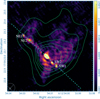 |
Fig. 1 Continuum image of the S255IR region. The intensity scale is in Jy beam−1. The contours show the low-resolution continuum emission. The contour levels are from 4 to 20 in steps of 4 mJy beam−1. The dashed line has a position angle of 47°. The four bright knots in the jet lobes are marked. The synthesized beams are shown in the lower left corner. |
3.2 Line emission
The observed bands cover many molecular lines. Here, we present observational results for several of the strongest and most informative lines, which help in understanding the structure, kinematics, and physical properties of this region.
3.2.1 C34S(7–6)
Fig. A.1 presents channel maps of the C34S(7–6) emission. The emission appears very clumpy. The velocity gradient is clearly seen in these maps. In Fig. 2, we present maps of the blueshifted and redshifted C34S (7–6) emission overlaid on the continuum image.
The C34S(7–6) emission in Fig. 2 clearly shows an elongated (almost perpendicular to the jet) and apparently rotating structure, which is most probably a disk-like object. Its extension along the major axis is about 400 AU. We generated a position–velocity (PV) diagram along this structure (the PV path is shown in Fig. 2), which is presented in the left panel of Fig. 3. The curves correspond to Keplerian rotation around the central mass of M sin2 i = 10 M⊙ (solid) and M sin2 i = 15 M⊙ (dashed), where i is the inclination angle. It is worth noting that the C34S(7–6) emission also extends along the jet and might indicate a velocity gradient across the jet (Fig. 2).
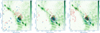 |
Fig. 2 Contours of the blueshifted and redshifted emission in the C34S(7–6) (left panel), SiO(8–7) (central panel), and CO(3–2) (right panel) line emission overlaid on the continuum image. The intensity scale is in units of Jy beam−1. The C34S(7–6) blue emission is integrated from −15 to −2 km s−1, and the C34S(7–6) red emission is integrated from 10 to 25 km s−1. The contour levels are 12, 19, 26, 33, and 40 mJy−1 beam−1 for the blueshifted emission and 15.0, 23.8, 32.5, 41.3, and 50.0 mJy beam−1 for the redshifted emission. The SiO(8–7) blue emission is integrated from −20 to 0 km s−1, and the SiO(8–7) red emission is integrated from 10 to 30 km s−1. The contour levels are 24, 38, 52, 66 and 80 mJy beam−1 for both blueshifted and redshifted emission. The CO(3–2) blue emission is integrated from −30 to −10 km s−1, the CO(3–2) red emission is integrated from 15 to 40 km s−1. The contour levels are 28.5, 39, 49.5, and 60 mJy beam−1 for the blueshifted emission and 38, 52, 66, and 80 mJy beam−1 for the redshifted emission. The cyan line shows the position of the PV cut (PA = 328°). The synthesized beams are shown in the lower left corners. |
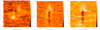 |
Fig. 3 Position-velocity diagrams for the C34S(7–6) (left panel), SiO(8–7) (central panel), and CO(3–2) (right panel) emission generated along the path shown in Fig. 2. The intensity scale is in mJy beam−1. The curves correspond to Keplerian rotation around the central mass of M sin2 i = 10 M⊙ (solid) and M sin2 i = 15 M⊙ (dashed), where i is the inclination angle. |
3.2.2 SiO(8–7)
The morphology of the SiO(8–7) emission is similar to that of the C34S(7–6) emission (Fig. 2), albeit apparently somewhat more compact along the disk and more extended along the blueshifted outflow lobe. The PV diagram in the SiO(8–7) line is presented in Fig. 3 (central panel). In this diagram, there is a prominent negative feature toward the central position that is broad in velocity; this feature is discussed in greater detail in Sect. 3.2.6.
3.2.3 CO(3–2)
The CO(3–2) emission in the vicinity of the central source (Fig. 2, right panel) exhibits approximately the same morphology as C34S(7–6) and SiO(8–7), but is much more extended along the outflow lobes. Particularly extended and bright emission is observed toward the redshifted lobe. The CO(3–2) emission along the continuum jet in the vicinity of the central source may indicate rotation. The PV diagram for the CO(3–2) emission along the same path as for C34S(7–6) and SiO(8–7) is shown in Fig. 3 (right panel). It also shows a strong negative feature toward the central position.
3.2.4 CH3CN(19–18)
The CH3CN(19–18) emission in this area is relatively weak at this high angular resolution and is confined to several compact regions. The strongest emission is observed in the disk and near the NE2 and SW2 knots in the jet.
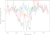 |
Fig. 4 Spectra of CO(3–2) (black), SiO(8–7) (red), C34S(7–6) (blue), and CH3CN(193−183) (green) toward the central source |
![Mathematical equation: $\[(\text{RA} = 6^{\mathrm{h}} 12^{\mathrm{m}} 54^\text{s}_\cdot0125, ~\text{Dec} =17^{\circ} 59^{\prime} 23^{\prime\prime}_\cdot053)\]$](/articles/aa/full_html/2024/12/aa52458-24/aa52458-24-eq9.png)
3.2.5 The methanol maser lines
We previously detected a new methanol maser line (141−140 A−+ at 349.1 GHz) in this area (Zinchenko et al. 2017); this is also seen in these new data. However, now there is one additional line of this series in the observed bands, 121−120 A−+. This line also shows the maser effect. We will present and discuss these results in a forthcoming publication. The maser effect in the lines of this series could be a tracer of luminosity flares during high-mass star formation (Salii et al. 2022).
3.2.6 Absorption features
As noted above, strong and wide absorption features are observed in the SiO(8–7) and CO(3–2) lines toward the central source. Figure 4 presents the spectra of all the lines at this central position and discussed above. An absorption, although much narrower, is also observed in C34S(7–6) and perhaps also in CH3CN(19–18).
The deepest absorption in the C34S(7–6), SiO(8–7), and CO(3–2) lines is seen at VLSR ~ 10 km s−1. In the CO(3–2) line, this absorption is about −800 K. At the same time, there are emission features at about −5 km s−1 in C34S(7–6) and CH3CN(193−183), and at about 20 km s−1 in CO(3–2) and SiO(8–7).
4 Discussion
4.1 General morphology
The results presented above very clearly show a rotating disk-like structure around the NIRS3 protostar and the jet originating in this structure. We must note that the orientation of this jet is significantly different from that observed at larger scales. According to the relatively old IR data, the PA of the jet axis is ≈67° (Howard et al. 1997). A similar orientation has been observed in several other works (Zinchenko et al. 2015; Cesaroni et al. 2018; Obonyo et al. 2021). This PA differs by ≈20° from that displayed in Fig. 1. However, recent observations at small scales show a jet orientation similar to that reported above. Cesaroni et al. (2023) found a PA for the jet of 48°, which almost perfectly coincides with our result. A very similar orientation was found by Hirota et al. (2021) from observations of water masers. These results indicate the disk precession as suggested in some previous works (Obonyo et al. 2021; Cesaroni et al. 2023). It is worth noting that this precession can result not only in a change of the PA of the outflow but also in a change of the inclination angle. This inclination angle is believed to be about 80°, that is, the disk is seen almost edge-on (Boley et al. 2013). However, it can change by about the same amount as the PA. It is not excluded that the large opening angle of the molecular outflow from the SMA1 clump (Zinchenko et al. 2015, 2020) can be explained by these variations of the jet orientation. The orientation of the extended redshifted CO(3–2) emission (Fig. 2) is closer to the PA of the outflow observed at large scales.
Our data show two pairs of bright knots in the jet, one in the each lobe. These pairs of knots were observed in the same areas as the NE and SW knots in Cesaroni et al. (2023) in 2021, which is approximately contemporaneous with our observations. In those observations, these pairs of knots were seen as single entities, apparently due to a much lower angular resolution. According to our data, the projected distance between the NE knots is 138 AU and between the SW knots it is 93 AU. The projected expansion speed is estimated as ~450 km s−1 for the NE lobe (Fedriani et al. 2023; Cesaroni et al. 2023) and ~285 km s−1 for the SW lobe (Cesaroni et al. 2024). Therefore, the observed distances between the knots correspond to about 530 days for the NE pair of knots and to about 570 days for the SW pair. Most probably, the presence of these two pairs of knots implies two events of ejection from the central source with the time interval of ~550 days or 1.5 years; it may also imply two events of accretion, respectively. The 6.7 GHz methanol maser (Szymczak et al. 2018) and NIR (Uchiyama et al. 2020) light curves exhibit complex behavior during the two years following the original burst. The light curve of the 6.7 GHz methanol maser at 2.87 km s−1 has two peaks with the same time interval between them (Szymczak et al. 2018), which is consistent with the assumption of two ejection events.
4.2 Nature of the continuum emission
4.2.1 The central source
The high brightness of the central source as well as its morphology (an elongation along the jet axis) hint at free-free emission of the ionized gas, but a dust contribution is not excluded. Liu et al. (2020) found the dust emission to be optically thin, with a brightness temperature of ~120 K at the ![Mathematical equation: $\[0^{\prime\prime}_\cdot 14\]$](/articles/aa/full_html/2024/12/aa52458-24/aa52458-24-eq10.png) scale. In principle, the dust column density and brightness can be higher at higher resolution. On the other hand, the contribution of the free-free emission to the measurements at the lower resolution should be non-negligible. The deep absorption in the molecular lines (Fig. 4) favors a bright compact central source.
scale. In principle, the dust column density and brightness can be higher at higher resolution. On the other hand, the contribution of the free-free emission to the measurements at the lower resolution should be non-negligible. The deep absorption in the molecular lines (Fig. 4) favors a bright compact central source.
Cesaroni et al. (2023) reported the flux densities for S255IR NIRS3 at several frequencies measured at different epochs. The latest measurements at most frequencies were performed in 2018. The data at 92.2 GHz were obtained in September 2021, at about the same time as our observations. The beam size in 2018 measurements was from ![Mathematical equation: $\[2^{\prime\prime}_\cdot 3\]$](/articles/aa/full_html/2024/12/aa52458-24/aa52458-24-eq11.png) at 3 GHz to
at 3 GHz to ![Mathematical equation: $\[0^{\prime\prime}_\cdot 2\]$](/articles/aa/full_html/2024/12/aa52458-24/aa52458-24-eq12.png) at 45.5 GHz. In the measurements at 92.2 GHz, the synthesized beam was
at 45.5 GHz. In the measurements at 92.2 GHz, the synthesized beam was ![Mathematical equation: $\[0^{\prime\prime}_\cdot 087\]$](/articles/aa/full_html/2024/12/aa52458-24/aa52458-24-eq13.png) . This beam also covers the SW2 knot. In our data, the flux integrated in the circle of
. This beam also covers the SW2 knot. In our data, the flux integrated in the circle of ![Mathematical equation: $\[0^{\prime\prime}_\cdot 09\]$](/articles/aa/full_html/2024/12/aa52458-24/aa52458-24-eq14.png) in diameter is ~60 mJy. However, this flux could include a significant contribution from the surrounding dust emission. Obonyo et al. (2021) reported fluxes for this object in 2018 of 24.72 ± 0.80 mJy at 22 GHz and 15.11 ± 0.09 mJy at 6 GHz, which are very similar to those measured by Cesaroni et al. (2023). The beam sizes were about
in diameter is ~60 mJy. However, this flux could include a significant contribution from the surrounding dust emission. Obonyo et al. (2021) reported fluxes for this object in 2018 of 24.72 ± 0.80 mJy at 22 GHz and 15.11 ± 0.09 mJy at 6 GHz, which are very similar to those measured by Cesaroni et al. (2023). The beam sizes were about ![Mathematical equation: $\[0^{\prime\prime}_\cdot 1\]$](/articles/aa/full_html/2024/12/aa52458-24/aa52458-24-eq15.png) and
and ![Mathematical equation: $\[0^{\prime\prime}_\cdot 28\]$](/articles/aa/full_html/2024/12/aa52458-24/aa52458-24-eq16.png) at 22 GHz and 6 GHz, respectively. Figure 5 shows the fluxes reported by Cesaroni et al. (2023) and our total flux of the central clump and the SW2 knot. It is necessary to bear in mind that the measurements were made at different times and with different beams.
at 22 GHz and 6 GHz, respectively. Figure 5 shows the fluxes reported by Cesaroni et al. (2023) and our total flux of the central clump and the SW2 knot. It is necessary to bear in mind that the measurements were made at different times and with different beams.
The shape of the spectrum in Fig. 5 is highly typical of a mixture of free-free and dust emission. Assuming an optically thin free-free emission with a spectral index of −0.1 at frequencies of ≳22 GHz, we obtain a free-free flux at 340 GHz of about 19 mJy from the measurements at 22.2 and 45.5 GHz (Cesaroni et al. 2023). This value can be considered as an upper limit for the optically thin free-free emission of the ionized gas in the central source because the measurements in Cesaroni et al. (2023) refer to an area including this source and the SW lobe. Our total flux for the knots in the SW lobe is 14.7 ± 1.8 mJy (Table 1). If it were fully attributed to the free-free emission, the share of the central source would be only ~4 mJy. The map of the free-free emission at 92.2 GHz in Cesaroni et al. (2024, their Fig. 3b) shows the brightness at the central source position of ~8 mJy beam−1. Therefore, for further estimates, we can consider the range of the free-free flux from the central source – assuming optically thin emission – to be ~4–19 mJy from 50.5 mJy (Table 1). The most probable value would be ~7 mJy, in accordance with the measurements at 92.2 GHz at the same epoch as our observations.
It should be noted that Cesaroni et al. (2024) obtained that only 14.6 mJy from 23.5 mJy at 92.2 GHz in this area refer to the free-free emission, while these authors attribute the remaining 8.9 mJy to the dust emission. In this case, the spectral index of this emission (attributed to dust) between 92 and 340 GHz is ~1.5, which is not consistent with the optically thin dust emission or even with the black body emission. We consider possible reasons for this discrepancy below.
In the framework of the model of the optically thin free-free emission of the ionized gas and dust emission, in terms of brightness temperature, assuming the same spatial distribution of both components, the obtained estimates of the fluxes imply a brightness of the free-free emission of ~70–320 K and a brightness of the dust emission of ~530–780 K (in our beam). However, such a simple summation would only be valid in the case of low optical depth for both components. The optical depth for the free-free emission in this picture is small, but the same is not true for the dust. The value of even ~530 K is much higher than the brightness of the dust emission in the ![Mathematical equation: $\[0^{\prime\prime}_\cdot 14\]$](/articles/aa/full_html/2024/12/aa52458-24/aa52458-24-eq17.png) beam (Liu et al. 2020) and implies a very high dust temperature. The upper limit for the dust temperature is the sublimation temperature, which is ~1500–2000 K for graphite and ~1000–1500 K for silicates (Churchwell et al. 1990). Such temperatures can be reached at the inner boundary of the dust cocoon around a massive star. This implies a substantial dust optical depth. At the same time, the optical depth of the central core cannot be too high, because we see emission features in the spectra in Fig. 4. These emission features should arise in the gas located behind the central core. For the dust optical depth of ~1, the dust temperature should be ≳850 K. This is a very high value but is probably not excluded in the vicinity of the massive YSO, which has a luminosity of a few times 104 L⊙. Under the same assumptions regarding dust opacity as in Liu et al. (2020), the dust optical depth of τ ~ 1 implies a hydrogen column density of N ~ 2 × 1025 cm−2 and a volume density of n ~ 3 × 1010 cm−3. It is worth noting that Liu et al. (2020) derived a gas density of ~6.6 × 109 cm−3 in the
beam (Liu et al. 2020) and implies a very high dust temperature. The upper limit for the dust temperature is the sublimation temperature, which is ~1500–2000 K for graphite and ~1000–1500 K for silicates (Churchwell et al. 1990). Such temperatures can be reached at the inner boundary of the dust cocoon around a massive star. This implies a substantial dust optical depth. At the same time, the optical depth of the central core cannot be too high, because we see emission features in the spectra in Fig. 4. These emission features should arise in the gas located behind the central core. For the dust optical depth of ~1, the dust temperature should be ≳850 K. This is a very high value but is probably not excluded in the vicinity of the massive YSO, which has a luminosity of a few times 104 L⊙. Under the same assumptions regarding dust opacity as in Liu et al. (2020), the dust optical depth of τ ~ 1 implies a hydrogen column density of N ~ 2 × 1025 cm−2 and a volume density of n ~ 3 × 1010 cm−3. It is worth noting that Liu et al. (2020) derived a gas density of ~6.6 × 109 cm−3 in the ![Mathematical equation: $\[0^{\prime\prime}_\cdot 14\]$](/articles/aa/full_html/2024/12/aa52458-24/aa52458-24-eq18.png) beam. However, if we consider the value of the dust absorption coefficient for “naked” dust at a density of 108 cm−3 from Ossenkopf & Henning (1994), the estimates of the hydrogen column and volume densities decrease by an order of magnitude.
beam. However, if we consider the value of the dust absorption coefficient for “naked” dust at a density of 108 cm−3 from Ossenkopf & Henning (1994), the estimates of the hydrogen column and volume densities decrease by an order of magnitude.
The brightness of the free-free emission of ~70–320 K (unaffected by the dust absorption) implies an optical depth of ~ 0.007–0.03 for a typical gas temperature of ~10 000 K. Then, using the well-known formulae for free-free emission (e.g., Wilson et al. 2013), we obtain an emission measure of EM~(0.5–2)×1010 pc cm−6. For the source size of ~40 AU, this implies an electron density of ne ~ (0.5–1)×107 cm−3. Such properties are typical of hypercompact H II regions (Kurtz 2005). For a uniform mixture of gas and dust, these estimates imply a very low ionization fraction. It is not excluded that dust is at least partly expelled from the ionized region and forms a dusty cocoon around it. When the size of the ionized gas emission region is smaller than the size of the dust emission region, the relative brightness of the free-free emission in the center will be higher.
An alternative model for this source can be based on a hypercompact H II region with a turnover frequency of ≳200 GHz, which can provide the spectral index of ~1.5 derived above for the excess emission in the frequency range of 92–340 GHz due to the decrease in electron density with radius (Kurtz 2005). This implies an emission measure of EM ≳ 2 × 10¹¹ pc cm−6. Such a model resolves the problem with the spectral index in the range of 92–340 GHz, but predicts an excessively high brightness temperature, taking into account the observed source size (as the optical depth at 340 GHz will be rather high). The solution could include dust absorption. Observations at several frequencies with sufficiently high resolution are required to select the most appropriate model.
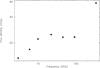 |
Fig. 5 Measured fluxes of S255 NIRS3 from Cesaroni et al. (2023) (from 3 to 92.2 GHz) and this work (340 GHz). At 340 GHz, a total flux of the central clump and the SW2 knot is plotted. |
4.2.2 Knots in the jet
Now, let us consider the emission of the knots in the jet. In Fig. 6 we present zoomed-in views of the NE and SW knots in continuum as well as in the C34S(7–6) and CH3CN(193−183) lines. There is no molecular emission associated with the NE1 or SW1 knots, while emission peaks in these lines are observed in the vicinity of the NE2 and SW2 knots.
Figure 7 shows the C34S(7–6) and CH3CN(193−183) line spectra in the regions marked in Fig. 6. It is worth noting that the velocities of the gas emitting in the C34S(7–6) and CH3CN(193−183) lines are somewhat different. In the NE (redshifted) lobe, the CH3CN(193−183) line is redshifted relative to the C34S(7–6) line, while in the SW (blueshifted) lobe, it is blueshifted. The C34S(7–6) velocities in the NE and SW lobes are close to each other. These features suggest that the C34S(7–6) emission arises mainly in the ambient gas, while the CH3CN(193−183) emission is also formed in the gas entrained by the jet. The brightness temperature in the lines reaches ~200 K in the NE lobe and ~300 K in the SW lobe. These values represent lower limits for the kinetic temperature of the emitting gas.
Cesaroni et al. (2023, 2024) presented and discussed detailed multi-frequency observations of the jet in the vicinity of the NIRS3 source. As mentioned above, these authors detected the NE and SW knots as single entities, in contrast to our data (due to a significantly lower angular resolution in their observations). They found that the free-free emission of the ionized gas dominates at frequencies of ≲30 GHz (the highest frequency was about 92 GHz). The fluxes at 92.2 GHz measured in September 2021 are 18.8 mJy for the NE knot and 23.4 mJy for the SW knot. Cesaroni et al. (2023, 2024) estimate that the flux of the SW free-free emission is 14.6 mJy after subtraction of the dust contribution, which could be somewhat questionable. Our total flux for the NE1+NE2 is 14.8 ± 1.9 mJy (obtained by summation of the values in Table 1). This value, within the uncertainties, is consistent with optically thin free-free emission. However, it is higher than in the model for the free-free emission suggested in Cesaroni et al. (2024). Our low-resolution continuum map (Fig. 1) shows a peak at the NE2 position. The flux density in this map integrated in the circle of ~250 mas in diameter around this peak is about 35 mJy. This appears to include a contribution from the surrounding dust. The situation with the SW knots is less clear, because Cesaroni et al. (2023, 2024) report total fluxes of our central clump and the SW knots. In our data, the emission of the SW knots is very similar in appearance to that of the NE knots and we believe that it can be interpreted in the same way. The emission measure of the knots in our data can be estimated as EM ~ 6 × 10⁹ pc cm−6, which implies a turnover frequency of ~30 GHz. This is approximately consistent with the spectra presented in Cesaroni et al. (2024). The electron density is about the same as in the central core, ne ~ 5 × 106 cm−3.
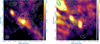 |
Fig. 6 Zoomed-in images of the NE (left panel) and SW (right panel) jet lobes in continuum at 0.9 mm overlaid with contours of the C34S(7–6) (green) and CH3CN(193−183) (yellow) integrated line intensity. The contour levels are 12.5, 21.9, 31.3, 40.6, and 50 mJy beam−1 km s−1 for both C34S(7–6) and CH3CN(193−183). The cyan ovals show the regions where the C34S(7–6) and CH3CN(193−183) spectra presented in Fig. 7 were extracted. The synthesized beams are shown in the lower left corners. |
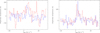 |
Fig. 7 Spectra of the C34S(7–6) (blue) and CH3CN(193−183) (red) emission in the NE (left panel) and SW (right panel) jet lobes in the regions indicated in Fig. 6. |
4.3 Kinematics of the material in the disk
The PV diagrams in several lines (Fig. 3) indicate sub-Keplerian rotation, as was found by Liu et al. (2020). Moreover, the earlier data presented in Zinchenko et al. (2015) lead to the same conclusion if the edge-on orientation of the disk is assumed. We do not question the estimates of the mass of the protostar, which was derived from the bolometric luminosity.
The absorption spectra presented in Fig. 4 show the deepest feature at VLSR ~ 10 km s−1, which is redshifted with respect to the systemic velocity of this core (VLSR ~ 5 km s−1). Therefore, it could be produced by the infalling material. As mentioned in Sect. 3.2.6, there is an emission feature at about −5 km s−1 in C34S(7–6) and CH3CN(193−183). This could be related to the infalling material behind the core.
5 Conclusions
In this paper, we present observations of the actively investigated high-mass star-forming region S255IR, which harbors the ~20 M⊙ protostar NIRS3. We achieve an angular resolution of ~15 mas, which corresponds to ~25 au and is almost an order of magnitude better than in the previous studies of this object. The observations were performed with ALMA at 0.9 mm in continuum and in several molecular lines. Our main results can be summarized as follows:
1. In continuum, we detect a central bright source (brightness temperature ~850 K) elongated along the jet direction and two pairs of bright knots in the jet lobes. The distances between the knots in the pairs correspond to a time interval of ~1.5 years, taking into account the previously determined velocities of the knots. This time interval coincides with the interval between the 6.7 GHz maser emission peaks at a certain velocity. It probably implies a double ejection from NIRS3 several years ago;
2. The orientation of the jet differs by ~20° from that on larger scales, as mentioned also in some other recent works. This implies a strong jet precession;
3. The 0.9 mm continuum emission of the central source represents a mixture of the dust thermal emission and free-free emission of the ionized gas. For the ionized gas, assuming optically thin emission at frequencies of ≳22 GHz, we obtain tn emission measure of EM~(0.5–2)×1010 pc cm−6 and an electron density of ne ~ (0.5–1)×107 cm−3. Such properties are typical of hypercompact H II regions. For a uniform mixture of gas and dust, these estimates imply a very low ionization fraction. It is not excluded that dust is at least partly expelled from the ionized region and forms a dusty cocoon around it. An alternative model for this source could be based on a hypercompact H II region with a turnover frequency of ≳200 GHz, which would better explain the spectral index in the range of 92–340 GHz, but has a problem with matching the observed brightness temperature. Observations at several frequencies with sufficiently high resolution are required to select the most appropriate model. In the continuum emission of the knots in the jet, the free-free component apparently dominates;
4. In the C34S(7–6), SiO(8–7), and CO(3–2) lines, we observe a rotating disk around NIRS3 of about 400 au in diameter. The rotation is sub-Keplerian. There are absorption features in the molecular lines towards the central bright source. The deepest absorption features are redshifted relative to the core velocity, which may indicate an infall;
5. The molecular line emission appears very inhomogeneous at small scales, which may indicate small-scale clumpiness in the disk;
6. Molecular emission is observed in the vicinity of the knots in the jet that are closer to the central source. In the NE (redshifted) lobe, the CH3CN(193−183) line is redshifted relative the C34S(7–6) line, while in the SW (blueshifted) lobe, it is blueshifted. The C34S(7–6) velocities in the NE and SW lobes are close to each other. These features suggest that the C34S(7–6) emission arises mainly in the ambient gas, while the CH3CN(193−183) emission is also formed in the gas entrained by the jet.
This system is obviously undergoing rapid evolution. Regular monitoring at several frequencies with high angular resolution would be very important for better understanding of the process of massive star formation.
Acknowledgements
This work was supported by the Russian Science Foundation grant number 24-12-00153 (https://rscf.ru/en/project/24-12-00153/). We are grateful to Stan Kurtz for the helpful discussions and to the anonymous referee for the useful comments. This paper makes use of the following ALMA data: ADS/JAO.ALMA #2019.1.00315.S. ALMA is a partnership of ESO (representing its member states), NSF (USA), and NINS (Japan), together with NRC (Canada), MoST and ASIAA (Taiwan), and KASI (Republic of Korea), in cooperation with the Republic of Chile. The Joint ALMA Observatory is operated by ESO, AUI/NRAO, and NAOJ.
Appendix A The C34S(7–6) channel maps
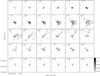 |
Fig. A.1 Channel maps of the C34S(7–6) emission in the S255IR region. The intensity scale is in Jy beam−1. The cross marks the phase center of the observations. |
References
- Boley, P. A., Linz, H., van Boekel, R., et al. 2013, A&A, 558, A24 [NASA ADS] [CrossRef] [EDP Sciences] [Google Scholar]
- Brogan, C. L., Hunter, T. R., Towner, A. P. M., et al. 2019, ApJ, 881, L39 [NASA ADS] [CrossRef] [Google Scholar]
- Burns, R. A., Handa, T., Nagayama, T., Sunada, K., & Omodaka, T. 2016, MNRAS, 460, 283 [NASA ADS] [CrossRef] [Google Scholar]
- Caratti O Garatti, A., Stecklum, B., Garcia Lopez, R., et al. 2017, Nat. Phys., 13, 276 [CrossRef] [Google Scholar]
- Cesaroni, R., Moscadelli, L., Neri, R., et al. 2018, A&A, 612, A103 [NASA ADS] [CrossRef] [EDP Sciences] [Google Scholar]
- Cesaroni, R., Moscadelli, L., Caratti o Garatti, A., et al. 2023, A&A, 680, A110 [NASA ADS] [CrossRef] [EDP Sciences] [Google Scholar]
- Cesaroni, R., Moscadelli, L., Caratti o Garatti, A., et al. 2024, A&A, 683, L15 [NASA ADS] [CrossRef] [EDP Sciences] [Google Scholar]
- Chen, Z., Sun, W., Chini, R., et al. 2021, ApJ, 922, 90 [NASA ADS] [CrossRef] [Google Scholar]
- Churchwell, E., Wolfire, M. G., & Wood, D. O. S. 1990, ApJ, 354, 247 [NASA ADS] [CrossRef] [Google Scholar]
- Fedriani, R., Caratti o Garatti, A., Cesaroni, R., et al. 2023, A&A, 676, A107 [NASA ADS] [CrossRef] [EDP Sciences] [Google Scholar]
- Hirota, T., Cesaroni, R., Moscadelli, L., et al. 2021, A&A, 647, A23 [NASA ADS] [CrossRef] [EDP Sciences] [Google Scholar]
- Howard, E. M., Pipher, J. L., & Forrest, W. J. 1997, ApJ, 481, 327 [NASA ADS] [CrossRef] [Google Scholar]
- Hunter, T. R., Brogan, C. L., MacLeod, G., et al. 2017, ApJ, 837, L29 [NASA ADS] [CrossRef] [Google Scholar]
- Kurtz, S. 2005, in Massive Star Birth: A Crossroads of Astrophysics, eds. R. Cesaroni, M. Felli, E. Churchwell, & M. Walmsley, IAU Symposium, 227, 111 [NASA ADS] [CrossRef] [Google Scholar]
- Liu, S.-Y., Su, Y.-N., Zinchenko, I., Wang, K.-S., & Wang, Y. 2018, ApJ, 863, L12 [Google Scholar]
- Liu, S.-Y., Su, Y.-N., Zinchenko, I., et al. 2020, ApJ, 904, 181 [Google Scholar]
- Meyer, D. M.-A., Vorobyov, E. I., Kuiper, R., & Kley, W. 2017, MNRAS, 464, L90 [NASA ADS] [CrossRef] [Google Scholar]
- Meyer, D. M. A., Vorobyov, E. I., Elbakyan, V. G., et al. 2019, MNRAS, 482, 5459 [Google Scholar]
- Moscadelli, L., Sanna, A., Goddi, C., et al. 2017, A&A, 600, L8 [NASA ADS] [CrossRef] [EDP Sciences] [Google Scholar]
- Motte, F., Bontemps, S., & Louvet, F. 2018, ARA&A, 56, 41 [NASA ADS] [CrossRef] [Google Scholar]
- Obonyo, W. O., Lumsden, S. L., Hoare, M. G., Kurtz, S. E., & Purser, S. J. D. 2021, MNRAS, 501, 5197 [NASA ADS] [CrossRef] [Google Scholar]
- Ojha, D. K., Samal, M. R., Pandey, A. K., et al. 2011, ApJ, 738, 156 [CrossRef] [Google Scholar]
- Ossenkopf, V., & Henning, T. 1994, A&A, 291, 943 [NASA ADS] [Google Scholar]
- Padoan, P., Pan, L., Juvela, M., Haugbølle, T., & Nordlund, Å. 2020, ApJ, 900, 82 [NASA ADS] [CrossRef] [Google Scholar]
- Proven-Adzri, E., MacLeod, G. C., Heever, S. P. v. d., et al. 2019, MNRAS, 487, 2407 [Google Scholar]
- Rosen, A. L., Offner, S. S. R., Sadavoy, S. I., et al. 2020, Space Sci. Rev., 216, 62 [Google Scholar]
- Salii, S. V., Zinchenko, I. I., Liu, S.-Y., et al. 2022, MNRAS, 512, 3215 [NASA ADS] [CrossRef] [Google Scholar]
- Szymczak, M., Olech, M., Wolak, P., Gérard, E., & Bartkiewicz, A. 2018, A&A, 617, A80 [NASA ADS] [CrossRef] [EDP Sciences] [Google Scholar]
- Tan, J. C., Beltrán, M. T., Caselli, P., et al. 2014, Protostars and Planets VI, 149 [Google Scholar]
- Tapia, M., Roth, M., & Persi, P. 2013, in Protostars and Planets VI Posters [Google Scholar]
- Uchiyama, M., Yamashita, T., Sugiyama, K., et al. 2020, PASJ, 72, 4 [NASA ADS] [CrossRef] [Google Scholar]
- Wang, Y., Beuther, H., Bik, A., et al. 2011, A&A, 527, A32 [NASA ADS] [CrossRef] [EDP Sciences] [Google Scholar]
- Wilson, T. L., Rohlfs, K., & Hüttemeister, S. 2013, Tools of Radio Astronomy (Springer) [CrossRef] [Google Scholar]
- Wolf, V., Stecklum, B., Caratti o Garatti, A., et al. 2024, A&A, 688, A8 [NASA ADS] [CrossRef] [EDP Sciences] [Google Scholar]
- Zinchenko, I., Liu, S.-Y., Su, Y.-N., et al. 2015, ApJ, 810, 10 [NASA ADS] [CrossRef] [Google Scholar]
- Zinchenko, I., Liu, S.-Y., Su, Y.-N., & Sobolev, A. M. 2017, A&A, 606, L6 [NASA ADS] [CrossRef] [EDP Sciences] [Google Scholar]
- Zinchenko, I. I., Liu, S.-Y., Su, Y.-N., Wang, K.-S., & Wang, Y. 2020, ApJ, 889, 43 [NASA ADS] [CrossRef] [Google Scholar]
- Zinchenko, I. I., Liu, S. Y., Ojha, D. K., Su, Y. N., & Zemlyanukha, P. M. 2024, arXiv e-prints [arXiv:2408.03133] [Google Scholar]
All Tables
All Figures
|
Fig. 1 Continuum image of the S255IR region. The intensity scale is in Jy beam−1. The contours show the low-resolution continuum emission. The contour levels are from 4 to 20 in steps of 4 mJy beam−1. The dashed line has a position angle of 47°. The four bright knots in the jet lobes are marked. The synthesized beams are shown in the lower left corner. |
| In the text | |
|
Fig. 2 Contours of the blueshifted and redshifted emission in the C34S(7–6) (left panel), SiO(8–7) (central panel), and CO(3–2) (right panel) line emission overlaid on the continuum image. The intensity scale is in units of Jy beam−1. The C34S(7–6) blue emission is integrated from −15 to −2 km s−1, and the C34S(7–6) red emission is integrated from 10 to 25 km s−1. The contour levels are 12, 19, 26, 33, and 40 mJy−1 beam−1 for the blueshifted emission and 15.0, 23.8, 32.5, 41.3, and 50.0 mJy beam−1 for the redshifted emission. The SiO(8–7) blue emission is integrated from −20 to 0 km s−1, and the SiO(8–7) red emission is integrated from 10 to 30 km s−1. The contour levels are 24, 38, 52, 66 and 80 mJy beam−1 for both blueshifted and redshifted emission. The CO(3–2) blue emission is integrated from −30 to −10 km s−1, the CO(3–2) red emission is integrated from 15 to 40 km s−1. The contour levels are 28.5, 39, 49.5, and 60 mJy beam−1 for the blueshifted emission and 38, 52, 66, and 80 mJy beam−1 for the redshifted emission. The cyan line shows the position of the PV cut (PA = 328°). The synthesized beams are shown in the lower left corners. |
| In the text | |
|
Fig. 3 Position-velocity diagrams for the C34S(7–6) (left panel), SiO(8–7) (central panel), and CO(3–2) (right panel) emission generated along the path shown in Fig. 2. The intensity scale is in mJy beam−1. The curves correspond to Keplerian rotation around the central mass of M sin2 i = 10 M⊙ (solid) and M sin2 i = 15 M⊙ (dashed), where i is the inclination angle. |
| In the text | |
|
Fig. 4 Spectra of CO(3–2) (black), SiO(8–7) (red), C34S(7–6) (blue), and CH3CN(193−183) (green) toward the central source |
| In the text | |
|
Fig. 5 Measured fluxes of S255 NIRS3 from Cesaroni et al. (2023) (from 3 to 92.2 GHz) and this work (340 GHz). At 340 GHz, a total flux of the central clump and the SW2 knot is plotted. |
| In the text | |
|
Fig. 6 Zoomed-in images of the NE (left panel) and SW (right panel) jet lobes in continuum at 0.9 mm overlaid with contours of the C34S(7–6) (green) and CH3CN(193−183) (yellow) integrated line intensity. The contour levels are 12.5, 21.9, 31.3, 40.6, and 50 mJy beam−1 km s−1 for both C34S(7–6) and CH3CN(193−183). The cyan ovals show the regions where the C34S(7–6) and CH3CN(193−183) spectra presented in Fig. 7 were extracted. The synthesized beams are shown in the lower left corners. |
| In the text | |
|
Fig. 7 Spectra of the C34S(7–6) (blue) and CH3CN(193−183) (red) emission in the NE (left panel) and SW (right panel) jet lobes in the regions indicated in Fig. 6. |
| In the text | |
|
Fig. A.1 Channel maps of the C34S(7–6) emission in the S255IR region. The intensity scale is in Jy beam−1. The cross marks the phase center of the observations. |
| In the text | |
Current usage metrics show cumulative count of Article Views (full-text article views including HTML views, PDF and ePub downloads, according to the available data) and Abstracts Views on Vision4Press platform.
Data correspond to usage on the plateform after 2015. The current usage metrics is available 48-96 hours after online publication and is updated daily on week days.
Initial download of the metrics may take a while.