| Issue |
A&A
Volume 689, September 2024
|
|
|---|---|---|
| Article Number | A354 | |
| Number of page(s) | 20 | |
| Section | Astrophysical processes | |
| DOI | https://doi.org/10.1051/0004-6361/202348726 | |
| Published online | 27 September 2024 | |
Two-dimensional simulations of disks in close binaries
Simulating outburst cycles in cataclysmic variables
1
Institute of Astronomy and Astrophysics, University of Tübingen, Auf der Morgenstelle 10, 72076 Tübingen, Germany
2
Faculty of Physics, University of Duisburg-Essen, Lotharstraße 1, 47057 Duisburg, Germany
Received:
24
November
2023
Accepted:
11
July
2024
Context. Previous simulations of cataclysmic variables studied either the quiescence, or the outburst state in multiple dimensions or they simulated complete outburst cycles in one dimension using simplified models for the gravitational torques.
Aims. We self-consistently simulate complete outburst cycles of normal and superoutbursts in cataclysmic variable systems in two dimensions. We study the effect of different α viscosity parameters, mass transfer rates, and binary mass ratios on the disk luminosities, outburst occurrence rates, and superhumps.
Methods. We simulate non-isothermal, viscous accretion disks in cataclysmic variable systems using a modified version of the FARGO code with an updated equation of state and a cooling function designed to reproduce s-curve behavior.
Results. Our simulations can model complete outburst cycles using the thermal tidal instability model. We find higher superhump amplitudes and stronger gravitational torques than previous studies, resulting in better agreement with observations.
Key words: accretion / accretion disks / hydrodynamics / instabilities / binaries: close / stars: dwarf novae / novae / cataclysmic variables
© The Authors 2024
 Open Access article, published by EDP Sciences, under the terms of the Creative Commons Attribution License (https://creativecommons.org/licenses/by/4.0), which permits unrestricted use, distribution, and reproduction in any medium, provided the original work is properly cited.
This article is published in open access under the Subscribe to Open model. Subscribe to A&A to support open access publication.
1. Introduction
Dwarf nova outbursts are regularly occurring brightness variations of the gas disk around a white dwarf in cataclysmic variable systems (CVs). CVs are compact systems consisting of a white dwarf whose accretion disk is fed by a Roche-lobe-overfilling companion. They are divided into subclasses based on their outburst characteristics, we refer to Warner (2003) for a comprehensive overview and to Inight et al. (2023) for a more recent and compact overview and observational catalog of these systems.
CVs undergoing dwarf nova outbursts can be separated into two distinct populations by an orbital period gap at around 2.8 h (Schreiber et al. 2024). Assuming typical white dwarf masses of 0.8 M⊙ in CVs (Pala et al. 2022), one can convert the period gap into a mass ratio gap of donor star mass divided by white dwarf mass of q = Mdon/Mwd ≈ 0.3 (Inight et al. 2023). Below the period gap (at low mass ratios) resides the SU Ursae Majoris (SU UMa) category, which is characterized by two different types of recurring outbursts: Normal outbursts, lasting only for 2–20 days, have amplitudes between 2 and 5 mag, recurrence rates from 10 days to tens of years, and superoutbursts, which are 5–10 times longer and are 0.7, mag brighter, and occur every few normal outbursts. During a superoutburst, smaller brightness variations occur, called superhumps which have periods that are typically slightly larger than the binary period. For systems above the period gap, both superoutbursts and superhumps are rarely observed (Patterson et al. 2005).
To explain the normal outbursts, a thermal disk instability model has been developed based on opacity changes around the ionization temperature of hydrogen and the subsequent transition from a radiative to a convective disk (Meyer & Meyer-Hofmeister 1981). Mineshige & Osaki (1983) noted that a varying α viscosity parameter (Shakura & Sunyaev 1973) from 0.01 during the quiescent phase to 0.1 during the outburst phase is needed to explain the observed cycles. This increase in α is attributed to the magnetorotational instability (MRI) (e.g. Lasota 2001, Sect. 2.4). First discovered by Velikhov (1959), Chandrasekhar (1960) for rotating cylinders and later rediscovered in the context of accretion disks by Balbus & Hawley (1991). However, it was only later confirmed in 3D magnetohydrodynamic (MHD) simulations that effective α values as high as 0.1 can be reached by convection-enhanced MRI (Oyang et al. 2021; Pjanka & Stone 2020). It should be noted that these high α values were obtained in local shearing box simulations and global MHD simulations often find lower values (Oyang et al. 2021; Pjanka & Stone 2020).
Coleman et al. (2016) used the viscosity-temperature relation found in Hirose et al. (2014) in 1D CVs simulations and were able to successfully simulate outburst cycles, but they also found sawtooth-like reflares during their outbursts that are not observed.
In the thermal-tidal disk instability (TTI) (Osaki 1989), superoutbursts are thought to be caused by an increase in the tidal torques when the disk grows to the 3:1 resonance radius during a normal outburst. For SU Uma systems (q ⪅ 0.3), the 3:1 resonance is located at ≈0.45 times the binary separation. If the disk grows to this size, it becomes tidally unstable and eccentric (Lubow 1991; Kley et al. 2008). The tidal torques cause the disk to shrink and release additional gravitational energy, which can explain the increased outburst duration and luminosity (Osaki 1989). In this model, the superhump phenomenon is caused by the precession of the eccentric disk (Whitehurst 1988). Observations of superoutbursts and superhumps in systems well above the period gap such as U Gem are seen as a challenge to the TTI (Smak & Waagen 2004) as the disks are expected to be smaller than the resonances that cause tidal torques. Although more recent observations of U Gem do find features that are consistent with tidal dissipation (Echevarría et al. 2023). In addition, Smak (2009b,a) argued that the TTI fails to explain the magnitude of the superhumps and proposed a superoutburst model based on a varying mass transfer rate from the donor star. However, there are no known mechanisms that can increase the mass transfer rate by several orders of magnitude, which would be required to explain the outbursts without the TTI.
A more recent issue with the TTI is brought up by global inviscid 3D MHD simulations (Ju et al. 2017). They find that angular momentum transport through spiral shocks and MRI produces less eccentric disks than simulations using the α viscosity model with the same effective αeff parameter. This is also confirmed by Oyang et al. (2021). They also explicitly show that the magnetic forces reduce the eccentricity of the disk, opposite to the viscous forces used in the α prescription, which are supposed to approximate the MRI.
However, there are concerns that the MRI is currently not properly resolved in global MHD simulations, resulting in numerical diffusivity that suppresses the MRI and potentially changing its behavior altogether (Nixon et al. 2024).
This work is a continuation of Kley et al. (2008) who were the first to use a grid code to study eccentric disks in close binaries. Using a locally isothermal model with constant kinematic shear viscosity, they studied the eccentricity growth rates of the disk. They found that the viscosity is positively correlated with the eccentricity growth rate and the final equilibrium eccentricity, that the inner boundary condition has a strong effect on the disk eccentricity, and that the mass stream can stabilize the disk and prevent eccentricity growth for low viscosity parameters. The aspect ratio h = H/r (ratio between the scale height of the disk and the distance to the central white dwarf), as an indicator of the pressure forces in the gas, and the tidal interaction with the binary determine the precession rate of the disk, as expected from theoretical models (Goodchild & Ogilvie 2006). Kley et al. (2008) also found that the eccentricity growth rate and equilibrium value are maximized for a specific aspect ratio and decrease for lower or higher aspect ratios. This result is reproduced in similar studies of protoplanetary disks in close binaries (Marzari et al. 2012; Jordan et al. 2021). Following the analysis presented in Lubow (1991), Kley et al. (2008) studied the mode coupling of the binary potential with the disk. By removing the m = 3 Fourier mode from the gravitational potential, they showed that it is the dominant but not the only mode driving eccentricity growth. This analysis of the contributions of the individual modes to the eccentricity growth was confirmed and expanded upon in Oyang et al. (2021).
In this study, we conduct two-dimensional vertically non-isothermal hydrodynamical simulations using the α viscosity prescription and a sophisticated equation of state that accounts for the dissociation and ionization of hydrogen, adopted from Vaidya et al. (2015). In addition, we have implemented the cooling function that reproduces the S-shaped equilibrium curve during CVs outbursts by Ichikawa & Osaki (1992) and the α scaling by Ichikawa et al. (1993). We use this code to perform a parameter study on the unknown parameters of the disk instability model and describe their effect on the outburst cycle of CVs.
Our paper is organized as follows: In Sect. 2 we reiterate the thermal tidal instability model, in Sect. 3 we describe our physical model, in Sect. 4 we describe our fiducial model and its outburst cycle, in Sect. 5 we change different parameters, one at a time, and study their effect on the outburst cycle and superhumps, and summarize our results in Sect. 6.
2. Disk instability model
In a cataclysmic variable system, the donor star overflows its Roche lobe, causing mass to be pushed from its surface towards the white dwarf through the inner L1 point between the two stars (Lubow & Shu 1975). Due to the conservation of angular momentum, the gas starts to form a disk at the circularization radius, and an over-dense ring forms at the outer edge of the disk.
The disk is initially in a cold, radiative state. Due to the viscous heating, the temperature inside the disk increases along with the gas density and eventually exceeds the ionization temperature of hydrogen, causing the opacity to increase. The high opacity prevents the disk from cooling efficiently and causes the disk to become convective and angular momentum transport is increased.
This transition from a cold to a hot state is called thermal instability, which can start either inside the outer density ring or near the white dwarf and expand until the entire disk is in an outburst state. In the outburst state, the angular momentum transport is increased due to the higher temperature. Additionally, the α parameter is also increased, which is necessary to match observations (Mineshige & Osaki 1983; Smak 1984). The beginning of such an outburst can be seen in the first panel in Fig. 1. Due to the increased angular momentum transport during the outburst state, the disk expands and loses mass until the density and temperature in the outer ring drop low enough to revert to the cold state, launching a cooling wave, which sweeps over the disk and resets it to the quiescent state.
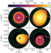 |
Fig. 1. Two-dimensional snapshots of the mid-plane temperature before and during a superoutburst for our fiducial setup, whose parameters are listed in Table 1. The cyan circle indicates the 3:1 resonance and the green line indicates the Roche lobe. The time in days is measured from the beginning of the outburst and one day is equal to 14.1 binary orbits (1.7 h). The simulation ran in a corotating reference frame, with the donor star fixed on the right side. |
In the tidal-thermal instability (TTI) model, the disk expands beyond a critical radius during an outburst (cf. second panel in Fig. 1), which increases the tidal torques acting on the disk. The tidal torques cause eccentricity growth (see third panel) and tidal dissipation which raises the temperature of the disk and prolongs the outburst (Whitehurst 1988; Kley et al. 2008; Oyang et al. 2021). The brightness variations known as superhumps can then be explained by the donor star moving past the bulge of the eccentric, precessing disk.
3. Numerical model
We perform two-dimensional non-isothermal hydrodynamic simulations of a cataclysmic variable system using the α viscosity prescription (Shakura & Sunyaev 1973). The simulations include the circumstellar accretion disk around the white dwarf and the gas transfer stream from the donor star. The system is assumed to be coplanar and the donor star is in a circular orbit around the white dwarf, while both stars are treated as point masses. For the disk, we solve the equations under the assumption of the restricted 3-body problem in the rotating frame of reference of the system, with the origin fixed at the position of the white dwarf. Consequently, gas feels the gravitational potential of the binary system and the indirect force due to the gravitational pull of the donor star on the white dwarf. We neglect the self-gravity of the gas and the gravitational feedback of the gas on the binary system. We use an updated version of the FARGO code (Masset 2000; Baruteau 2008) for our simulations.
The FARGO code is based on the ZEUS2D code (Stone & Norman 1992), which uses an explicit second-order upwind scheme on a staggered grid for advection and an operator splitting technique to solve the source terms of the Navier-Stokes equations. All derivatives are first order in space and time. To improve the treatment of shocks in the used upwind scheme, we apply the artificial viscosity by Tscharnuter & Winkler (1979) to ensure the correct jump conditions through the shock front and the correct shock velocity. The scale height of the gas is computed from the gravity of both stars (compare Günther et al. 2004) and we reduce the viscosity of specific cells at the outer edge of the disk for numerical stability. Test cases and the implementation of all the modules we use are described in detail in Rometsch et al. (2024). The code and our fiducial setup are publicly available under AGPLv3 on github1.
3.1. Physical basics
The code solves the vertically integrated hydrodynamic equations in polar coordinates (r,ϕ) in the mid-plane (z = 0). The coordinate system is centered on the white dwarf and in the corotating frame of reference of the binary. The gas velocity is given as v = (vr,rΩ), where omega is the angular velocity in the corotating frame. We used the standard momentum equations and refer to Rometsch et al. (2024) for details on the implementation. The energy equation is given by
where e is the vertically integrated internal energy density, P the vertically integrated pressure, v the gas velocity and Q+ and Q− are the heating and cooling source terms.
We used a non-perfect ideal equation of state (EoS) that accounts for hydrogen ionization and dissociation. The implementation of this EoS follows Vaidya et al. (2015). It uses multiple adiabatic indices to relate thermodynamic quantities. The effective adiabatic index γeff relates the vertically integrated pressure P to the internal energy density e:
where R = kB/mH is the specific gas constant, Σ is surface density, Tmid is the mid-plane temperature, and μ is the mean molecular weight. The temperature inside the cell is assumed to be vertically isothermal and is labeled as Tmid to distinguish it from the brightness temperature Teff at the surface of the disk. The relation for the speed of sound, using the first adiabatic index Γ1, is given by

where Σ is the surface density. The gas is heated by viscous heating due to shear viscosity and shock dissipation due to artificial viscosity:
![$$ \begin{aligned} Q_+ = \frac{1}{2 \nu \Sigma } \left[ \sigma _{rr}^2 + 2 \sigma _{r \phi }^2 + \sigma _{\phi \phi }^2 \right] + \frac{2 \nu \Sigma }{9} \left( \nabla \boldsymbol{v} \right)^2 + Q_\mathrm{art} , \end{aligned} $$](/articles/aa/full_html/2024/09/aa48726-23/aa48726-23-eq4.gif)
where σij are the coefficients of the viscous stress tensor in polar coordinates, ν = αHcs is the kinematic shear viscosity according to Shakura & Sunyaev (1973), Qart is the shock heating due to our artificial viscosity, which is implemented as an artificial pressure (see Appendix B Stone & Norman 1992) and behaves the same as bulk viscosity. We use an artificial viscosity constant of  in all our simulations and the only sources of shocks, where shock heating will be active, are the spiral waves due to the interaction with the binary potential and the impact of the gas stream on the disk.
In our early tests, we found that a constant αcold parameter tended to produce outbursts that start inside and move outward, with outside-in outbursts only occurring in simulations with high mass transfer rates. However, observations show that many outbursts are outside-in (Vogt 1983). We have therefore copied the solution of Ichikawa et al. (1993) for this problem and used a varying αcold for all simulations in this work:
with αcold, 0 = 0.01 − 0.04, which is in the range deduced from the recurrence times from observations α ⪅ 0.01 (Cannizzo et al. 2012) and more recent MRI simulations α ≈ 0.03 (Hirose et al. 2014; Scepi et al. 2018). An outwardly increasing α parameter is supported by the observations of Mineshige & Wood (1989).
By fitting a viscous model to observational data, Kotko & Lasota (2012) found that the alpha viscosity parameter should be of the order of αhot ≈ 0.1 − 0.2.
The increase in angular momentum transport as the disk transitions from the quiescent to the outburst state was modeled by a temperature-dependent α parameter, which changes smoothly from αcold to αhot for increasing temperatures and vice versa for decreasing temperatures. We followed the approach of Ichikawa & Osaki (1992), where α is given by
![$$ \begin{aligned} \log {\alpha } =&\log {\alpha _\mathrm{cold} }\nonumber \\&+ \frac{1}{2} \left( \log {\alpha _\mathrm{hot} - \log {\alpha _\mathrm{cold} } } \right) \left[ 1 - \tanh {\frac{4 - \log {T_\mathrm{mid} / \mathrm{K} }}{0.4}} \right], \end{aligned} $$](/articles/aa/full_html/2024/09/aa48726-23/aa48726-23-eq7.gif)
where Tmid is the mid-plane temperature in Kelvin, the transition between αcold and αhot occurs around Tmid = 104 K. For cooling, we used the prescription from Ichikawa & Osaki (1992). The model divides the cooling function into a cold radiative branch, a hot convective branch, and an intermediate branch. For the cold branch, they used opacities based on Cox & Stewart (1969) and a flux of

for the optically thin regime to derive the radiative flux through the surface of the disk:
where τ is the optical depth, σSB is the Stefan-Boltzmann constant. For this formula, all quantities are given in cgs units. The cold branch applies to temperatures Tmid < TA, where TA is the temperature at which
The radiative losses of the hot branch were derived using a one-zone model for an optically thick disk:

Using Kramer’s law for the opacity of ionized gas, the radiative flux through the surface of the disk can be approximated as

where again this expression is in cgs units. The hot branch is valid for temperatures Tmid > TB, where TB is the temperature at which
where log FB/[erg s−1 cm−2]=K(r) is an approximation for the flux at the start of the hot branch based on Fig. 3 in Mineshige & Osaki (1983):
![$$ \begin{aligned} K(r) = 11 + 0.4\, \mathrm{log } \left[ \frac{2\cdot 10^{10} \,\mathrm{cm} }{r} \right]. \end{aligned} $$](/articles/aa/full_html/2024/09/aa48726-23/aa48726-23-eq14.gif)
The radiative losses in the intermediate branch are given by an interpolation between the hot and cold branches:
![$$ \begin{aligned} \mathrm{log} \, {F}_\mathrm{int} = (\mathrm{log} \, F_A / [\mathrm{erg} \, \mathrm{s} ^{-1} \mathrm{cm} ^{-2}] - K(r)) \mathrm{log} \, \frac{T_c}{T_B} /\, \mathrm{log} \,\frac{T_A}{T_B} + K(r). \end{aligned} $$](/articles/aa/full_html/2024/09/aa48726-23/aa48726-23-eq15.gif)
This interpolation formula is only valid for FB > FA, cases where FB < FA are handled by setting FB = FA and Fint = FA. The radiative losses due to surface cooling are then given by QcoolTI = 2F where F is the radiative flux pieced together from the cool, intermediate, and hot branches as described above.
The surface cooling inside the intermediate branch has a weaker dependence on the disk temperature than the viscous heating of Eq. (4). If the disk enters the intermediate branch from the cold branch, it will heat up faster the hotter it is, leading to runaway heating. If the disk enters the intermediate branch from the hot branch, it will cool faster the colder it is, resulting in runaway cooling. This is the intended effect of the cooling prescription used in disk instability models, as it leads to outbursts and subsequent return to quiescence. It also allows us to predict the conditions necessary to start an outburst by looking at Eq. (7). The mean molecular weight and the gas temperature are self-consistently solved in the code, leaving only the surface density and the angular velocity as parameters that can trigger an outburst. For this reason, studies of the disk instability model often define a critical surface density at which an outburst is triggered. The critical surface density can also be converted into a critical temperature by a heating model and into a critical mass accretion rate by an angular momentum transport model (Lasota et al. 2008).
Since the white dwarf mass is fixed in our study, the critical surface density of our model is only a function of the distance to the white dwarf through Ω ∝ r−3/2, meaning that at larger radii higher surface densities and higher temperatures are needed to trigger an outburst. Physically, this dependence of the model is explained by the fact that the outburst starts with the onset of convection in the disk (Meyer & Meyer-Hofmeister 1981), which depends not only on the opacity of the gas, but also on the vertical gravity, for which the white dwarf is the dominant source.
The cooling prescription from Ichikawa & Osaki (1992) was developed for conditions inside the accretion disk, and we found that it is not suitable to handle the low-density regions outside the truncation radius. Therefore, we used a different cooling technique at low densities:
where Q−, rad is the surface cooling according to Hubeny (1990) with the opacity table from Lin & Papaloizou (1985). The change of the cooling prescription is done only for numerical stability reasons and has a negligible effect on the overall simulation.
Fig. 2 shows a comparison of the model from Ichikawa & Osaki (1992) for our fiducial parameters with the more recent values from MRI simulations (Scepi et al. 2018). The top panel shows the thermal equilibrium curve for which the models agree near the instability (at Σ ≈ 200 g/cm2) and in qualitative agreement further away from the instability. The bottom panel shows the α parameter as a function of the mid-plane temperature. Here, the models are in good agreement in the cold state and during the transition to the hot state. After the transition to the hot state, shearing box MRI simulations find that the turbulence becomes weaker again. This is thought to happen because the opacity in the ionized state is given by Kramers law κ ∝ T−7/2, which decreases with increasing temperature, quenching the convection (Hirose et al. 2014; Scepi et al. 2018). We also ran simulations with the MRI-based α prescription from Coleman et al. (2016), but found reflares after the outbursts. We chose the bimodal α prescription over the MRI-based one because it more accurately reproduces observations where reflares are uncommon. For a discussion of these different α prescriptions, we refer to Coleman et al. (2016).
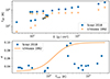 |
Fig. 2. Top panel: thermal equilibria [Teff] vs. [Σ] from the shearing box simulations in Scepi et al. (2018) (data taken from their Table 1) and the model from Ichikawa & Osaki (1992) for the same input parameters. Bottom panel: the measured α parameters in Scepi et al. (2018) and the interpolation function Eq. (6) as a function of the mid-plane temperature. |
3.2. Numerical considerations
We used a fixed white dwarf mass of Mwd = 0.765 M⊙ and a fiducial mass of Mdon = 0.092 M⊙ for the donor star. This gives us a fiducial mass ratio of q = Mwd/Mdon = 0.12 and an inner Lagrange L1 point at L1 = Rmax = 0.7abin, which we used as the outer radius of our simulation domain. We then changed the mass ratio by changing the mass of the donor star while adjusting the outer radius of the domain accordingly. The minimum radius of our domain is always Rmin = 0.05 abin ≈ 2.2 ⋅ 109 cm and was chosen for legacy reasons and the high computational cost of reducing it. The inner radius is three times the radius of the white dwarf, assuming a radius of Rwd = 0.73 ⋅ 109 cm (Mathew & Nandy 2017). Our inner radius could be interpreted as the radius within which the disk is rapidly emptied by magnetic winds. Magnetic winds produce a roughly constant inner radius, while optical winds are not expected to truncate the disk during the outburst state (Tetarenko et al. 2018). According to Scepi et al. (2019), the radius of the magnetic wind-dominated region is
where μ30 = μ/(1030G cm3), Ṁ16= Ṁtr/1016 g s−1M1 = Mwd/M⊙. Assuming an average mass accretion rate equal to our fiducial mass transfer rate of Ṁtr = 1.5 · 10−10 M⊙/yr ≈ 1016 g s−1, we find a magnetic dipole moment of 1.2μ30 for our inner domain radius. The dipole moment can be translated into a magnetic field strength of B = μRwd3 ≈ 3 kG, which is a weak magnetic field for a white dwarf (Landstreet et al. 2016).
We initialized all of our models with a constant surface density of Σ0 = 8.7 g cm−2 throughout the domain. This results in an initial disk mass of Md = 2 ⋅ 10−11Mwd ≈ 3 ⋅ 1022 g, which is roughly the disk mass after a superoutburst for our fiducial model. For numerical stability, we used a density floor of Σfloor = 10−8 ⋅ Σ0 as the minimum surface density for the simulation. If a cell fell below this surface density, it was reset to the floor value. Similarly, we used a temperature floor of 10 K and a temperature ceiling of 3 ⋅ 105 K. All cells outside the tidal truncation radius are typically at the density floor at all times, but we did not notice any cells reaching either the temperature floor or the temperature ceiling.
3.3. Analysis
All disk quantities were measured as snapshots during the simulation at a rate of 100 times per binary orbit. In this section we define the disk quantities used in the evaluation which consist of eccentricity, longitude of pericenter, luminosity, mass, radius, aspect ratio, and the torque exerted by the gas on the donor star. In addition to these quantities, we have also tracked the mass leaving through the inner and outer boundaries during our simulations.
For specific time frames of the fiducial model, we measured the gravitational torque density using the formula by Miranda et al. (2017):
where Φ is the smoothed gravitational potential of the binary system in the frame of the white dwarf:

where G is the gravitational constant, ϵ = 0.6 H is the gravitational smoothing length (Müller et al. 2012), and H is the disk scale height. The last term in the potential is the indirect term caused by the donor star accelerating the white dwarf.
The torque Γz exerted by the disk on the donor star, which was monitored during all simulations, is calculated in Cartesian coordinates as follows
![$$ \begin{aligned} \Gamma _z = M_\mathrm{don} \left[\mathbf r _\mathrm{don} \times \int G \Sigma \frac{\mathbf{r - \mathbf r _\mathrm{don}} }{\left. \sqrt{\left| \mathbf r - \mathbf r _\mathrm{don} \right|^2 + \epsilon ^2}\right.^3} \mathrm{d} x~\mathrm{d} y \right]\cdot \hat{e}_z. \end{aligned} $$](/articles/aa/full_html/2024/09/aa48726-23/aa48726-23-eq20.gif)
Note that this torque is only measured, not applied to the stars. Compared to the torque exerted on the disk by the binary, this torque has the opposite sign and does not take into account the effects of the indirect term on the gas. For this reason, we made only a qualitative evaluation of the donor star torque.
The disk luminosity is computed by integrating the radiative losses Q− from Eq. (14) over the surface of the disk:
We have noticed several luminosity peaks in our data. We believe that these are caused by numerical instabilities at the outer edge of the disk, where strong density gradients occur. Therefore, we have replaced individual exceptionally bright data points with the average of the two neighboring points.
If the luminosity gradient at the top of a luminosity peak was exceptionally high, we removed the data points from our dataset, up to a maximum of five data points per luminosity peak. This only affected a few superhumps at the beginning of a superoutburst.
We calculated the effective temperature, or brightness temperature, of a gas cell as
![$$ \begin{aligned} T_\mathrm{eff} = \left[\frac{Q_-}{2 \sigma _\mathrm{SB} }\right]^{1/4}, \end{aligned} $$](/articles/aa/full_html/2024/09/aa48726-23/aa48726-23-eq22.gif)
and used this temperature to compare against the brightness temperatures measured from observations.
The eccentricity of the disk and the longitude of pericenter ωd are calculated as a mass-weighted average. We used the same formulation as in previous studies (e.g. Kley et al. 2008):
where Md is the total disk mass:
Our disk radius is defined as the radius of the ring containing 99% of the total disk mass when the mass is integrated from the innermost to the outermost ring.
For the evaluation, we used only data starting after the first outburst to remove the effects of our initial conditions. We used smoothing to reduce the noise in spontaneously measured quantities such as disk eccentricity, longitude of periastron, the aspect ratio, or the disk radius, which oscillate on timescales of the binary period. The quantities were smoothed in two passes. The first pass smoothed the quantities with a Hamming window two binary periods wide, and the second pass with a window one binary period wide.
3.4. Boundary conditions
We used strict outflow boundaries at the inner boundary and strict outflow boundaries at the outer boundary, except for the small region around the Lagrange L1 point where the mass inflow stream originates. At each boundary, the azimuthal velocity was always set to the pressure-supported Keplerian velocity:
where h = 0.002 was assumed to be constant, which is the aspect ratio we typically find in our simulations during the quiescence state. The energy and surface density were set to zero gradient conditions and the radial velocity was zero gradient for outflow from the domain and zero for inflow.
We computed the width of the mass stream using the approximation function in Warner (2003, Sect. 2.4.1), assuming a stream temperature of Tstream = 1500K. We then smoothed the mass stream with a Gaussian profile over three times its width. We have found that the initial stream width and temperature are unimportant, since both quickly reach a new equilibrium upon entering the simulation domain. Identical to Kley et al. (2008), we set the initial radial velocity of the mass stream to be 2 ⋅ 10−3 vK(abin), where vK(abin) is the Keplerian velocity of the donor star. Then we set the surface density to a value that produces the desired mass inflow rate Ṁtr.
We ran one simulation with a variable mass flow rate from the donor star, using the prescription by Hameury et al. (2000). It is supposed to model the increase in mass transfer due to the illumination of the donor star by the disk and the accretion luminosity of the white dwarf during the outburst. While there is observational support for an increase in mass transfer by a factor of two during outbursts (Smak 1995), models on irradiation of the donor star do not agree on the increase in mass transfer, see Osaki & Meyer (2004) or Viallet & Hameury (2008) and Cambier (2015). Following Hameury et al. (2000), we based the mass transfer rate on the accretion rate of the white dwarf:
where b is a free parameter for which we used 0.5 (Hameury et al. 2000). To reduce the noise in the white dwarf mass accretion Ṁacc, we computed the current mass accretion as an exponentially weighted moving average:
where dt is the timestep length, ΔMacc is the mass that has left the domain through the inner boundary during the timestep, and c = dt/tavg where tavg = 10Tbin and  is the mass accretion rate from the previous step.
3.5. Boundary test
In this section, we present a locally isothermal model to evaluate our choice of boundary conditions. The disk is initialized with a mass of Md = 2 ⋅ 10−11Mwd and mass transfer is disabled. The model used a constant aspect ratio of h = 0.03 and a constant viscosity parameter of α = 0.1 to model a disk in the outburst state. The setup is similar to the one used in Kley et al. (2008) and therefore the disk eccentricity is expected to grow exponentially until the growth is balanced by mass ejection from the outer disk. The equilibrium eccentricity is determined by the aspect ratio and the viscosity parameter (Kley et al. 2008). We used strict outflow conditions at the inner and outer boundaries for the fiducial model.
In addition to the outflow conditions at the inner boundary, we tested the effect of reflecting inner boundary conditions and wave damping at the inner boundary by damping the azimuthal velocity and surface density to the azimuthally averaged values using the damping prescription by de Val-Borro et al. (2006) on damping time scales of 10−1, 3·10−2, and 10−2 orbital periods at the radius of the inner boundary. We also tested a viscous outflow condition where the surface density was set to zero gradient and the radial velocity to a constant times the viscous speed:
where νkin is the kinematic shear viscosity and s = 0.2, 15.
We also ran another test with mass transfer and another test where we moved the outer outflow boundary to 6 abin and applied wave damping inside the 3−6abin by damping the azimuthal velocity to the azimuthally averaged value, and the surface density and radial velocity to zero on a damping timescale of 10−1 orbital periods at the distance of the outer domain radius.
The time evolution of the mass-averaged disk eccentricity for all the different boundary conditions are shown in Fig. 3. The outer boundary conditions affect the growth rate and the time at which the eccentricity growth starts, but do not affect the equilibrium eccentricity. The simulation with the mass transfer stream starts its eccentricity growth at the beginning of the simulation. Its eccentricity grows faster than in the reference case without mass transfer. Similar results were found in Kley et al. (2008), but in our case the eccentricity growth is increased even more.
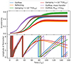 |
Fig. 3. Top panel: Disk eccentricity evolution for locally isothermal models with different boundary conditions. Bottom panel: Time evolution of the longitude of pericenter of the disk in radians. |
To compare the results, we define the start of eccentricity growth as the first time the eccentricity reaches 0.05 and the duration of eccentricity growth as the time it takes for the eccentricity to grow from 0.05 to 95% of its equilibrium value. Using these definitions, we find that eccentricity growth starts at 10 Tbin for the simulation with mass stream, and its growth time is 42 Tbin. The simulation with the outer boundary at 6 abin has a similar eccentricity growth time, 43 Tbin, but starts its growth at 26 Tbin. Both simulations eventually reach the same equilibrium eccentricity as the reference simulation. Simulations with the outer boundary at the inner L1 point all start their eccentricity growth around 32 Tbin with growth times ranging from 46 to 73 Tbin depending on the equilibrium eccentricity.
For the value of the equilibrium eccentricity, we find three distinct groups, depending on the inner boundary condition, with a representative of each group shown in Fig. 4. For evaluation, we used the radial profile of the azimuthally mass-averaged eccentricity (solid lines) and the azimuthally averaged surface density (dashed lines). All profiles were averaged over 20 snapshots taken between 140 and 160 binary periods.
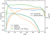 |
Fig. 4. Radial profiles of mass-weighted azimuthally averaged disk eccentricity and azimuthally averaged surface density. All profiles were also averaged over 20 simulation snapshots from simulation times 140 to 160 binary periods. |
The reflecting inner boundary simulation leads to a high density at the inner boundary, which then decays outward with a power-law profile until it is tidally truncated by the companion. We also find that the disk has a retrograde precession, which we attribute to the increased pressure forces due to the strong density gradient. The eccentricity is zero at the inner boundary and grows slowly with increasing radius, and the total disk eccentricity is the lowest of all our simulations. The same behavior was already found in Kley et al. (2008), except that in their study the simulation with the outflow boundary had the lowest eccentricity. We found similar results for the simulation with viscous outflow s = 0.2 and damping conditions with a damping time scale of τ = 10−2 orbital periods.
The simulation with a damping timescale of τ = 10−1 orbital periods, as well as the simulation with the viscous outflow with s = 15 has a constant radial surface density profile towards the inner region and a prograde precession. The eccentricity is still forced to zero at the inner boundary, but quickly rises to a high value that remains almost constant throughout the disk. The average disk eccentricity is the highest for our locally isothermal test runs.
The simulations with outflow at the inner boundary develop an inner eccentric hole as seen in Fig. 1 or by the density drop in Fig. 4. The disk also has a prograde precession. This is the only boundary condition that does not force the eccentricity to zero. The eccentricity at the inner boundary is high, but then drops to a lower level for the rest of the disk. The average disk eccentricity is lower than for the damped inner boundary, but still higher than for the reflecting boundary condition. The simulations with mass transfer stream or damping at the outer boundary have the same precession rate and produce the same radial profiles as the simulation with only outflow at the outer boundary.
Finally, we repeated the simulation with the outflow at the inner and outer boundaries, but with a reduced inner radius of 0.0167 abin, one third of the fiducial inner radius and equal to a typical white dwarf radius of Rwd = 7.3 ⋅ 109 cm. For the smaller inner radius we find an equilibrium eccentricity of 0.5, 6% higher than for the fiducial inner radius (e = 0.47), and a prograde precession rate of 0.068Pbin−1, 33% slower than for the fiducial model ( ). Higher eccentricity and faster retrograde precession are also found by Jordan et al. (2021) for smaller inner radii with a reflective inner boundary condition. We conclude that the outer boundary affects the eccentricity growth, but not the equilibrium eccentricity. From the boundaries tested, the mass transfer stream seems to have a stronger effect than moving the boundary outward and adding wave-damping regions at the outer boundary. Because the mass transfer is implemented as a boundary condition, the outer domain radius must be located at the inner L1 point for the mass transfer stream to work. Therefore, we cannot test the effect of both mass transfer and a larger outer domain radius at the same time. We therefore assume that both effects are independent and the effect of a larger outer domain radius is less relevant while the mass transfer stream is active.
It has been previously shown that the inner boundary has a significant influence on the outburst behavior of dwarf novae (Kley et al. 2008; Hameury & Lasota 2017; Scepi et al. 2019). Here we have shown that by using a damping zone near the inner boundary or by imposing a radial outflow velocity, one can smoothly transition from an outflow boundary that produces a prograde precessing disk to a reflective boundary that produces a retrograde precessing disk with lower eccentricity by adjusting either the damping timescale or the outflow velocity. Since we used different boundary conditions and obtained the same results, we conclude that the effects of the boundaries are due to the physical conditions they impose on the disk, and that the effects of numerical oscillations that occur when the boundaries are implemented using the primitive variables instead of the characteristic variables, as discussed in Godon (1996), are negligible.
4. Fiducial model
We adopted the physical parameters of the SU UMa dwarf nova system V1504 Cygni (Coyne et al. 2012) for our fiducial model. This system has been observed for a long period of time by the Kepler telescope and its light curves are well studied (Cannizzo et al. 2012; Osaki & Kato 2014). We acquired the Kepler data via the Python package Lightkurve (Lightkurve Collaboration 2018; Astropy Collaboration 2022). For the mass transfer rate, we choose a fiducial value of 1.5 × 10⁻¹⁰ M⊙/yr ≈ 1016 g/s which is within the range of transfer rates estimated from observations of dwarf novae systems below the period gap (Dubus et al. 2018). In these systems, mass transfer is thought to be caused by the loss of angular momentum of the binary due to gravitational radiation. For our fiducial mass ratio, we chose a value of q = 0.12, which is at the lower end of the estimates for V1504 Cygni by Coyne et al. (2012). The combination of mass transfer rate and mass ratio used in the fiducial model was chosen to produce an outburst supercycle comparable to observations of V1504 Cyg. The parameters for the fiducial model are summarized in Table 1. In Figure 5, we present several disk quantities over time for the fiducial model for the duration of a supercycle and the light curve of V1504 Cygni during a time frame with the same duration. The light curve shows a sequence of normal outbursts between two superoutbursts. Our simulated outburst amplitudes are generally larger than those observed. We have confirmed that this is due to our choice of cooling model, which we discuss at the end of this paper. We believe that this is caused by the low cooling on the hot branch of our model (Eq. (10)) leading to too high mid-plane temperatures. We see the effects of this several times throughout this paper.
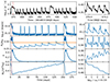 |
Fig. 5. The upper panels show Kepler data of V1504 Cygni over an equal length time frame as the simulated data below. The binary period is 1.7 hours, and one day is equal to 14.1 binary periods. The extent of the y-axis in the left panel is the same as in the plot below, but in the right panel, the extent of the y-axis is reduced by a factor of 3.8 compared to the plot below. Bottom left panel: Luminosity, disk radius, eccentricity, and total mass as a function of time for the fiducial model. The orange line indicates the 3:1 orbital resonance radius. The red dashed line indicates the time at which the right panel is zoomed in and the black dashed line indicates the start of the second superoutburst. Bottom right panel: Zoom in on the same quantities during a superoutburst as a function of the longitude of pericenter of the disk relative to the position of the binary. The angles are shifted by π and normalized so that integer values indicate that the binary passes the bulge of the eccentric disk. |
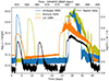 |
Fig. 6. Comparison of the luminosity curves for the fiducial model using the cooling prescription from Ichikawa & Osaki (1992) (blue line), the revised version of that cooling prescription from Kimura et al. (2020) (yellow line) and a model using surface cooling with opacities from (Lin & Papaloizou 1985) (orange line) as well as Kepler data of V1504 Cygni (black line). |
Parameters of the fiducial model.
Except for the first normal outburst after a superoutburst, successive normal outbursts increase in amplitudes, outburst duration, and duration of the quiescent phase. The density distribution of the disk after a superoutburst is affected by the ringing down from the highly eccentric state that developed during the superoutburst to the circular state during the quiescent phase. This effect is highlighted in Fig. 7 and leads to higher densities inside the disk. The additional mass inside the disk increases the outburst luminosity. This causes the first normal outburst after a superoutburst to be brighter than the next normal outburst. However, we observed this effect only in simulations with mass ratios of q = 0.25 or lower, and did not observe it for V1504 Cygni, with a few exceptions. This could be explained by the different quiescent periods after a superoutburst, which will affect the mass of the disk during the first normal outburst. We often find a long quiescent period after a superoutburst in our simulations, while observations of V1504 Cygni find short quiescent periods after superoutbursts.
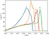 |
Fig. 7. Azimuthally averaged density distributions as a function of radius before (1, 2) and after (1′ and 2′) the first and second normal outbursts following a superoutburst. The solid lines are taken from the first and the dashed lines from the second supercycle of the fiducial model. |
Looking more closely at the luminosity during the quiescent phases, it can be seen that the quiescent luminosity increases with the disk mass. This effect follows directly from our viscous heating model since the viscous heating (Eq. (4)) is proportional to the surface density and, via the α viscosity prescription, also to the mid-plane temperature. This effect is also observed in other studies (e.g. Hameury et al. 1998) and is generally considered to be a weakness of these models (Hameury 2020). Since it is not found in observations.
The noise in the luminosity during the quiescence is caused by the hot spot where the mass stream impacts the disk. We restarted the simulation during the quiescence without the mass stream and found the luminosity to be nearly constant and 60% lower (corresponding to a drop of 0.4 on the log scale in the second panel of Fig. 5) than with the mass stream active. The average effective temperature of the hot spot is Teff ≈ 40 ⋅ 103 K with peak temperatures of 100 ⋅ 103 K, these values are significantly higher than the brightness temperatures measured from observations of up to 15 ⋅ 103 K for the OY carinae system (Wood et al. 1989).
The too high hot spot temperatures could be explained by the lack of in-plane radiative diffusion in our simulation and the 2D approach underestimates the spread of the stream. In addition, our viscosity and cooling model may not be applicable to the hot spot because they were developed for conditions inside the disk.
For the quiescent disk, Wood et al. (1989) measured brightness temperatures Teff of 4400 K at the center of the disk and 3300 K at the outer rim, while we measure 3000 K near the inner boundary and 2400 K near the outer rim and 4000 K inside the outer density ring in our simulations. During the initial rise of a superoutburst, we measure effective gas temperatures from 20 ⋅ 103 K near the inner boundary to 6 ⋅ 103 K at the outer boundary of the disk. Given our large inner boundary, which limits the disk extension towards the white dwarf, these temperatures are in good agreement with the brightness temperatures of 25 ⋅ 103 K to 6 ⋅ 103 K measured from OY Carinae during superoutbursts by Bruch et al. (1996) and Pratt et al. (1999).
We simulated our fiducial model for three supercycles and found no significant differences between the cycles. The precise periodicity of our supercycles is highlighted by the dashed lines in Fig. 7. It shows the density distribution during the normal outbursts after the second superoutburst and it exactly matches the density distributions measured after the first superoutburst.
Both the spiral waves during a superoutburst and the outer density ring in Fig. 7 could overflow the disk, similar to the hydraulic jumps at spiral waves observed in protoplanetary disks (Boley & Durisen 2006; Picogna & Marzari 2013). Both of these 3D effects could influence the mass transport in the disk and thus the outburst conditions, but are not included in our simulations.
4.1. Normal outbust
Fig. 8 shows the light curve and disk radius evolution of an outside-in and an inside-out outburst from our αcold = 0.04 model. The outburst starts when the disk reaches the intermediate branch in the Ichikawa & Osaki (1992) model at about Tmid ≈ 3000 K in the outer rim of the disk. In this regime, the cooling rates increase less with increasing temperature than the viscous heating, causing the temperature to rise faster.
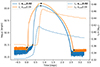 |
Fig. 8. Luminosity and disk radius evolution during a normal, outside-in outburst of our fiducial model (αcold = 0.02) and an inside-out outburst of our αcold = 0.04 model. Squares and dots indicate what we define as the start of the outburst, the start of the heating wave, the peak, and the end of the outburst. |
The temperature rise is initially slow and confined to the density ring around the disk which causes the slow rise at the beginning of the blue curve in Fig. 8. Once the temperature in the ring reaches Tmid ≈ 13 ⋅ 103 K, the α parameter of Eq. (6) grows rapidly and the temperature and α jump to Tmid ≈ 50 ⋅ 103 K and αhot and launch a heating wave inward, seen as the steep rise in luminosity and disk radius. Due to the disk spreading by angular momentum transport, the gas density and temperature at the outer edge drop below their critical values, and a cooling wave is launched that moves inward and causes the luminosity to drop and the disk to start shrinking.
Note that the outburst starts near the outer edge of the disk and two heating waves are launched, one traveling inward and one outward. But the outward wave quickly reaches the edge, while the inward wave traverses the majority of the disk. Therefore, we mention the inward wave only when the outburst starts in the outer rim and call it an outward-in outburst and similarly, we mention the outward wave only when the outburst starts in the inner disk and call it an inside-out outburst.
In the case of the inside-out outburst (Fig. 8, orange curve), the slow initial rise is much shorter and the heating wave travels at about half the speed of the outside-in wave. This gives the outburst a more symmetrical shape, which was already studied in Smak (1984). The growth of the disk radius is delayed until the heating wave has reached the outer edge of the disk. From this point on, the evolution is identical to the outside-in outburst. Whether an outburst starts inside-out or outside-in depends on whether the inward transport of gas by viscosity is more effective than the mass pileup at the outer rim (Lasota 2001, Sect. 4.4).
For comparison, the light curve of V344 Lyr during two consecutive outbursts is shown in Fig. 9. The presumed inside-out outburst of V344 Lyr (orange line) occurs after an unusually long quiescent period. The light curve also displays negative superhumps that could be caused by a tilted disk, which in turn would explain the long quiescent period. This would lead to a higher mass build-up and a higher outburst amplitude Cannizzo et al. (2012).
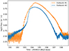 |
Fig. 9. Kepler luminosity data during two consecutive outbursts of V344 Lyr for comparison with Fig. 8. |
After the growth phase during the ourburst ends, the disk radius shrinks due to the accretion of low angular momentum gas from the mass stream. Overall we find a slow upward trend in the disk radius over time. Similarly, the eccentricity also increases slightly during each normal outburst and decreases during the quiescent state, also with a slow upward trend.
4.2. Superoutbust
With the steady increase in disk radius and eccentricity, the radius will exceed the 3:1 resonance at some point during an outburst, leading to significantly increased tidal forces. The gravitational torque density during the quiescent phase and the superoutburst is presented in Fig. 10. During the quiescent phase (blue line), the tidal torque is limited to the outer rim of the disk and has similar positive and negative contributions, such that the total tidal torque acting on the disk is weak and negative. During a superoutburst, the torques are amplified and reach further into the disk.
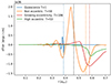 |
Fig. 10. Azimuthal and time-averaged (over 10 Pbin) gravitational torque density Eq. (16) during different stages of a superoutburst. The vertical dashed lines are the time-averaged disk radii during the same time frame. The black vertical line indicates the position of the 3:1 resonance. The legend also notes the total integrated torques exerted on the disk, normalized to the torque during quiescence. |
We measure strong negative torques at the outer rim that prevent the disk from expanding further and keep the outer parts optically dense and hot. In addition, the total torques are always negative and release additional tidal energies that heat the disk. Both effects prevent the cooling wave from being launched and thus prolong the outburst. The highest torque density amplitudes occur during the early stages of the superoutburst when the eccentricity is still low (orange line). The strongest total torques occur during the eccentricity growth phase (red line) and are almost two orders of magnitude stronger than during the quiescent phase. The disk is restructured and the eccentricity grows until the torques are again confined to the outer regions of disk (green line).
The 3:1 resonance seems to be a good reference radius at which the strength of the tidal interaction begins to increase and eccentricity begins to grow (see the second plot in Fig. 5), but recent studies have shown that the 3:1 resonance is not the only relevant mode for eccentricity growth (Kley et al. 2008; Oyang et al. 2021).
We compared the absolute values of the torques measured in Fig. 10 to the torque estimated due to our fiducial mass transfer rate via the approximation by King (1988, Eq. 8):
where

is the angular momentum of the binary. This equation assumes that the gas is transferred from the donor star to the white dwarf and the torque, when averaged over time, should be equal to the tidal torques measured in Fig. 10 plus the direct torque due to the mass stream.
We find a mass transfer torque Ttr = 2.4 ⋅ 1034 ergs, which is 21 times larger than the gas torque during quiesence and five times smaller than the peak gas torque during the superoutburst. Note that our binary system is on a fixed orbit, and the stars do not feel the effect of this angular momentum transport or gas accretion in our simulations.
Fig. 11 depicts a zoom in on several quantities during a superoutburst for our fiducial model and our variable mass transfer model, where the mass transfer rate was increased by a factor of about eight during the superoutburst. It demonstrates how the increased mass transfer rate dampens the eccentricity which reduces the mass loss and also provides mass during the outburst, resulting in a longer outburst. Without the increased mass transfer, the rapid luminosity decline causes the superhumps to appear to increase in amplitude.
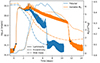 |
Fig. 11. Evolution of several quantities during a superoutburst for our fiducial model (blue) and variable mass transfer model using Eq. (24) (orange). The solid lines represent the disk luminosity while the dots and squares indicate the timestamps of the start, the peak, and the end of the outburst. Also shown are the mass-weighted disk eccentricity (dashed line) and the disk mass (dash-dotted line). |
The outbursts start as an outside-in outburst and then remain in the outburst state while the disk fills the entire Roche lobe of the white dwarf (see the second panel in Fig. 1). This phase lasts ≈1 day. During this phase the luminosity decreases due to mass loss and a decrease in gravitational interaction with the donor star (see also Fig. 12). Then the gravitational interaction suddenly increases, leading to higher luminosities, eccentricity growth, and the appearance of superhumps. After another ≈1 day has passed, the eccentricity reaches a value of e ⪆ 0.2 and the torque on the disk, the luminosity, and the superhump amplitudes reach their peaks.
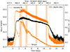 |
Fig. 12. Luminosity evolution during a superoutburst for our variable mass transfer model (orange line, same as in Fig. 11) and Kepler data of V1504 Cygni (black line). The shaded regions indicate the time frames presented in Fig. 14. The orange dashed line is the torque exerted by the disk on the donor star. No units are given for the torque because we are only making a qualitative assessment. |
The right panel in Fig. 5 shows a zoom-in around the red dashed vertical line in the left panel. The x-axis is the difference between the binary angle and the longitude of pericenter of the disk. It is shifted by π and normalized so that integers indicate the time at which the binary is flying past the bulge (apocenter) of the eccentric disk. Most of the mass loss occurs shortly after the apocenter passage, when the eccentricity and radius peak. In our fiducial model, 84% of the mass leaves the domain through the inner boundary and 16% is ejected through the outer boundary. During a normal outburst, only ≈3 ⋅ 10−3% of the mass is ejected. The mass that leaves the simulation domain through the outer boundary is either ejected from the system, reaccreted on the disk, or accreted on the donor star. Since the disk overflows the Roche lobe of the white dwarf during the superoutburst and the spiral arm of the disk extends towards the donor star in the third panel of Fig. 1, it seems likely that most of the ejected mass would be accreted by the donor star and interacts with its surface. For our simulation with a variable mass stream, we measure less eccentricity during the superoutburst and the amount of mass ejected through the outer boundary was reduced to 4% of the total mass loss.
After the disk has reached a highly eccentric state e ≥ 0.2, the surface area of the disk starts to exponentially decay (not shown) and the gravitational interaction with the donor star weakens. At this stage, any further eccentricity growth leads to an increase in the mass loss of the disk in addition to the viscous accretion (see the blue dashed-dotted line at t = 4 days in Fig. 11). Although the disk surface area shrinks, the disk radius remains relatively constant throughout the superoutburst, but one should keep in mind that our disk radius (defined as the smallest grid radius that contains 99% of the disk mass) is tracking the extent of the tip of the eccentric disk and not the semi-major axis of an ellipse.
The disk cools down until a cooling wave is launched at the outer rim and the disk quickly shrinks back to the 3:1 resonance radius. The disk still has a significant eccentricity e ≈ 0.3 after returning to the quiescent state, which then slowly dissipates and in some cases lasts until the next normal outburst. The dissipation of eccentricity also affects the density structure of the disk as shown in Fig. 7. In many of our simulations, we also find a small luminosity bump after the superoutburst (e.g. at t = 8 d in Fig. 11), coinciding with the phase of the fastest eccentricity decay.
The rapid luminosity decline of the fiducial superoutburst, the growth of superhump amplitudes during the decline, the flattening of the light curve before the end of the outburst, and the small luminosity bump afterward are all features that are not found in observations. The variable mass transfer solves these problems and better reproduces the observations. However, it is not clear from our simulations to what extent a variable mass transfer rate is necessary to reproduce the observations, because the effects described in our fiducial model can also be explained by the choice of the cooling prescription (see Fig. 6), the overestimation of the eccentricity due to simulating in 2D (compare Latter & Ogilvie (2006) or Oyang (2022, Ch. 4), and the overestimation in mass loss due to our too large inner boundary.
4.3. Superhumps
The top right plot in the bottom panel in Fig. 5 shows the disk luminosity as a function of the angle between the disk apocenter and the donor star. The x-axis is normalized so that integer numbers indicate the time at which the binary passes the bulge (apocenter) of the eccentric disk. The disk is slowly precessing prograde (Tprec ≈ 55Tbin) such that one unit of the normalized angle covers close to one binary period. As the donor star passes the apocenter of the disk, two spiral arms are launched that travel inward into the disk (visible in the second panel of Fig. 1) and dissipate energy. The energy dissipation starts after a delay of about 1/6 Tbin and is completed after another 1/3 Tbin.
We interpret and label these brightness variations as superhumps. In our fiducial model (blue line), we find an increase of factor two in superhump amplitudes in later stages of the superoutburst (see Fig. 11). This behavior is opposite to observed superhumps, which become weaker as the outburst progresses, as can be seen in Fig. 12 and Fig. 13. The increase in amplitude is caused by narrow luminosity peaks during the superhump. The peaks are caused by the high eccentricities and amplified by the rapid luminosity decline in our simulations. High superhump amplitudes caused by spikes in luminosity are usually discarded when analyzing superhump amplitudes (Kato et al. 2012, Sect. 4.7.1). Since all of our simulations with constant mass transfer rates develop superhump brightnesses with narrow peaks, we used the variable mass transfer model for our superhump analysis in this section and compared it to an observed superoutburst of V1504 Cygni.
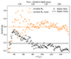 |
Fig. 13. Superhump amplitudes for the variable mass transfer model and V1504 Cygni measured from the data presented in Fig. 12. |
The light curve data used for the evaluation is presented in Fig. 12. The shaded regions indicate an arbitrary selection of time frames at different outburst stages. A zoom in on these time frames is given in Fig. 14, note that the plots cover different time scales while the y-axis is always fixed to cover a range of 0.26 log10L. The maxima and minima of these superhumps are marked by blue and green crosses, respectively. The superhump excess and amplitudes are later calculated from these extrema.
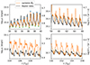 |
Fig. 14. Luminosity of the variable mass transfer model and Kepler data of V1504 Cygni during different phases of the superoutburst as indicated in Fig. 12. The time is measured from the start of the superoutburst. The crosses indicate the minima and maxima of the superhumps used in further evaluation. |
The first panel in Fig. 14 shows the onset of superhumps during the rapid eccentricity growth phase. Once the average disk eccentricity exceeds e > 0.1, the superhumps reach their full strength with a single, symmetrical peak. The second panel depicts the superhumps during the weaker eccentricity growth phase (at t = 58 Tbin ≈ 4 days in Fig. 11). In our simulations, the central peak is weakened for every second superhump which does not happen in the observed superhumps. In both cases, the superhumps become more asymmetric, with a fast rise and a slower decline in luminosity.
During the phase when the eccentricity has reached its maximum, the superhumps have a short, small peak with an almost flat plateau (third panel). We also find this behavior in the observed superhumps, but our simulations significantly overestimate the superhump amplitudes. At the end of the outburst (fourth panel), the minima between the superhumps become wider, in agreement with the observations. The observed superhump amplitudes become smaller while our simulated superhumps remain at a constant level and develop a double-peak structure.
4.3.1. Superhump excess
We calculated the superhump excess from the maxima and minima, shown in Fig. 16. The raw data is quite noisy and has a grid-like shape due to our quantity sampling rate of 100 times per binary orbit. The data is smoothed by convolving with a normalized Hamming window of size 20 (black dots), and the resulting curve tracks the disk precession rate (orange line), which is computed from the mass-weighted longitude of pericenter of the disk. The disk precession rate is plotted in Fig. 15.
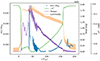 |
Fig. 15. The disk precession rate during a superoutburst, together with the torque exerted by the disk on the donor star and the negative of the gas aspect ratio squared. The luminosity curve in the background is for orientation only. |
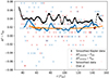 |
Fig. 16. Superhump excess calculated from adjacent peaks or minima for our variable mass transfer model (red or blue crosses, see the first panel in Fig. 14). The blue dots are an average of nearby data points and the orange dots are the precession rate of the disk. The black dots are the superhump excess computed from Kepler data of V1504 Cygni using an orbital period of 1.668 h (Coyne et al. 2012). |
Because our evaluation function averages the angle of the longitude of pericenter of all cells, we get incorrect results whenever the longitude of pericenter of the disk is close to 2π. We have filtered out the incorrect results, causing gaps in the precession rate curve. Our precession curve can be explained by the theoretical model by Goodchild & Ogilvie (2006), which predicts that gravitational forces cause prograde precession and pressure forces cause retrograde precession. After a short initialization phase, the precession timescale settles to about tprec = 50Pbin. From there, it slows down to tprec = 60Pbin due to a reduction in the gravitational interaction with the binary. As the disk cools down (seen as an increase in −h2), the pressure forces weaken and the prograde precession rate increases again.
The smoothed superhump excess computed from the Kepler data of V1504 Cygni (black dots) is similar in shape to our simulated superhump excess, but due to the noise in the data, we cannot confirm the trend described above. The superhump excess is, on average, larger than in our simulations, indicating again that our disks are too hot during the outburst state.
4.3.2. Superhump amplitudes
Fig. 13 shows the amplitudes from our variable mass transfer model that are calculated as (Smak 2009b):
We find alternating 0.3 and 0.6 amplitudes during the first half of the outburst t ⪅ 70 Pbin, which then transition to more stable amplitudes with a mean of A = 0.4. These amplitudes are a factor of four larger than the 2D simulations presented in Smak (2009b) and on average a factor of two larger than the observed superhumps. In this respect, our superhump amplitudes seem to be in agreement with the observed ones, since 3D simulations tend to find amplitudes that are lower by a factor of 2–4 than 2D simulations (Smak 2009b).
It should also be noted that the superhump amplitudes in our models arise purely from tidal dissipation within the disk and we could not find a relation between the mass transfer rate and the superhump amplitude. In Fig. 17, we compare the fiducial model during the high eccentricity phase of a superoutburst with a copy of the fiducial model that was restarted without any mass transfer from the donor star. By turning off the mass transfer, the superhump amplitudes even increase due to lower luminosity minima and higher second luminosity peaks.
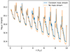 |
Fig. 17. Luminosity curves for the fiducial model during the high eccentricity phase of a superoutburst compared to a restart with the mass transfer turned off. |
4.3.3. Late superhumps
While the disk is still eccentric, the quiescent phase and normal outbursts following a superoutburst can also produce superhump-like brightness variations, called late superhumps. We find late superhumps in all our simulations, which are caused by the varying impact velocity of the mass stream on the eccentric disk. This is in agreement with Rolfe et al. (2001), who measured the shape of the accretion disk in the eclipsing dwarf nova system IY UMa and found an eccentric disk, and that the brightness variations of the system can be explained by a varying impact velocity of the mass stream.
We present the light curve of a normal outburst following a superoutburst for one of our simulations together with Kepler data of V344 Lyr in Fig. 18. We do not observe these variations for non-eccentric disks, as seen in the quiescent luminosities in Fig. 8. We also found that the brightness variations disappear when the mass stream is turned off while the disk is eccentric, as shown by the blue and orange lines in Fig. 18. This confirms that they are caused by the mass stream impacting an eccentric disk.
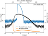 |
Fig. 18. Luminosities during the first normal outburst following a superoutburst. The black line presents Kepler data of V344 Lyr, the blue line is for our Ṁtr = 2.5 · 10−10 M⊙/yr model and the orange is a simulation of the same model but restarted with the mass transfer turned off. |
4.3.4. Hot spot luminosity
We extracted the luminosity of the hot spot by comparing the luminosities of the simulations with and without mass transfer in Fig. 18. For the quiescent luminosity with mass transfer, we measure Ld = 2.94 ⋅ 1031 ergs/s averaged from the start of the plot until time t = 0 d. The average luminosity without mass transfer is Ld = 0.89 ⋅ 1031 ergs/s measured from t = 0.5 d to t = 3.5 d. For the high mass transfer model depicted in Fig. 18, we find that the hot spot contributes Lhs = 2.05 ⋅ 1031 ergs/s to the total luminosity and is more than two times brighter than the disk itself.
The luminosity of the hotspot can also be estimated using the formula in Smak (2002):
where Mbin is the binary mass, abin is the binary separation, and Δu is a dimensionless equivalent of the impact velocity. Using the estimate for the Roche radius from Eggleton (1983) and q = 0.12, we find Δu2 ≈ 2 using the interpolation formula from Smak (2002). This results in an estimated hot spot luminosity of Limpact = 3.74 ⋅ 1031 ergs/s. The approximate hot spot luminosity is about twice as large as our measured hot spot luminosity, which could indicate that not all of the kinetic energy of the mass stream is converted into luminosity in our simulations. However, it should be noted that the shock heating is added to the heating source term and therefore does not conserve the total energy, but numerical errors of this magnitude seem unlikely.
Studies that decompose the light curves of eclipsing CVs also find hot spot luminosities that are comparable to the disk luminosity (Bąkowska & Olech 2015) or brighter than the disk luminosity (McAllister et al. 2019, Fig. 1). Our simulations do not include contributions to the light curve from the white dwarf, its boundary layer, and the donor star, which means that the total quiescent luminosity is underestimated and the importance of the disk and hot spot luminosities are overestimated.
4.3.5. Flickering
The noise in the quiescent luminosity in our simulations could be associated with the flickering found in observations. In our simulations, it is caused by random fluctuations in the hot spot that stop when the mass stream is turned off (see the orange line in Fig. 18). The residual oscillations for the simulation without mass transfer are caused by tidal dissipation due to the eccentric disk, and we confirmed that they do not occur for circular disks (not shown).
The amplitudes of these fluctuations caused by the mass stream depend, in addition to physical parameters, on the time step size of our integration scheme. We believe this is due to the compression and shock heating being added in a separate integration step from the surface cooling. This causes the temperature in the hot spot to overshoot the equilibrium temperature, which causes the surface cooling to be too effective in the next integration step, causing oscillations around the equilibrium temperature.
Therefore, it is likely that the agreement of the flickering amplitudes in our simulations with the observed amplitudes is coincidental. Note that this statement applies only to the flickering (random noise) in the quiescent luminosity, and not to the late superhumps depicted in Fig. 18, which we believe to be physical.
Observations of dwarf novae find that most of the flickering originates from a region close to the white dwarf, which is not included in our simulations, with additional contributions from the hot spot (Bruch 1996; McAllister et al. 2015). There are other proposed sources of flickering, but it is not yet clear which are the relevant ones. We refer to Bruch (2021) for a discussion of this topic.
5. Physical parameter study
In addition to the fiducial model, we ran 17 other simulations, where we changed one parameter from the fiducial model in each setup. The parameters that we changed are the viscosity parameters αhot and αcold, the mass transfer rate Ṁtr and the mass ratio q. All simulation parameters and characteristics of the superoutbursts are listed in Table 2.
Overview of all simulation parameters and the evaluation of superoutbursts.
5.1. Viscosity
The effect of different αhot parameters is shown in Fig. 19, where normal outbursts are marked with dots and superoutbursts with squares. The plot starts at the time of the second outburst because the first normal outburst was used as the initialization time. We performed the same analysis for two different outburst cycles from the Kepler data of V1504 Cyg, which is given in Fig. 20.
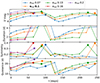 |
Fig. 19. The visual magnitude, duration, and symmetry of the outbursts, and the quiescent duration between outbursts for different αhot parameters. |
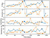 |
Fig. 20. Same as Fig. 19 but for Kepler data of V1504 Cyg. The two lines represent two different outburst cycles. |
Higher αhot causes the outbursts to evolve faster, the initial heating wave moving slightly faster across the disk and the cooling wave becoming significantly faster, reducing the duration of normal outbursts (second panel in Fig. 19). The larger increase in the cooling wave speed compared to the heating wave increases the symmetry of the normal outbursts, where the symmetry is defined as the time from launching the heat wave to the peak luminosity of the outburst divided by the total duration of the outburst (compare the markings in Fig. 8). The higher viscosity during the outburst state increases the radius growth so that there are fewer normal outbursts between superoutbursts as can be seen in the first panel where the first superoutburst occurs after four normal outbursts (including the first outburst not shown in the plot) for the high αhot = 0.16 and 0.2 simulations and six outbursts for the lowest αhot = 0.07 simulations.
In our model (see Equations (7), (8)), the temperature required for starting an outburst increases with radius while the temperature itself is proportional to the surface density due to viscous heating. Larger disk radii therefore lead to longer quiescent periods between outbursts.
The higher dissipation also increases the outburst luminosity, as shown by the increase in visual magnitude in the first panel of Fig. 19. Although for the superoutbursts, the peak luminosity is measured at the hump caused by the increased tidal interaction. At this time, the increase in mass loss due to higher viscosity counteracts the increase in viscous dissipation, and we find no trend in the amplitudes of superoutbursts. The faster mass loss also causes the disk to be cooler at the time when superhumps appear, leading to an overall faster disk precession or equally superhump excess (see Table 2). The superhump amplitudes are too noisy with too few data points to determine a trend and have magnitudes around 0.5 regardless of αhot. We have not used the second half of the superhump amplitudes, because the increase in superhump magnitude in later stages is not compatible with observations.
Comparing these results with the observed trends (Fig. 20), it is clear that dwarf novae systems have more variability in their outburst properties than our 2D simulations with a constant mass transfer rate. We can still see the increasing trend in brightness and duration for successive outbursts. The durations of the normal outbursts are best matched by the αhot = 0.07 and 0.1 models and the symmetry by the αhot = 0.1 and 0.13 models. However, it is important to note that this similarity is specific to this setup and that other parameters, namely the binary mass ratio, the mass transfer rate, and also the cooling prescription will affect the same outburst properties.
The αcold parameter only affects the disk during quiesence. It has little effect on the quiescent duration because the change in viscous dissipation is balanced by the change in mass transport. The effective temperature during the quiescent phase before a superoutburst changes from Teff ≈ 1900 − 2300 K (αcold = 0.01, inner disk to outer disk) to 2400 − 3000 K (αcold = 0.02) and 3200 − 3800 K (αcold = 0.04). The peak temperature in the density ring during the same time was Teff = 4200 K, independent of αcold. The increase in the quiescent luminosity reduces the visual magnitude compared to the following outburst, even though the absolute luminosity during the outbursts is the same. For αcold = 0.04, the mass transport through the disk is strong enough such that the outburst conditions are reached in the inner disk first, triggering an inside-out outburst, which is indicated by a cross in Fig. 21. The inside-out outbursts do not have the radius-quiescence relation of the outside-in outbursts, so the quiescence durations are random with a small spread instead of increasing monotonically.
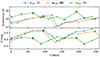 |
Fig. 21. Quiescent duration between outbursts for different αcold parameters. Dots indicate normal outbursts, crosses indicate inside-out normal outbursts, and squares indicate superoutbursts. |
5.2. Mass transfer rate
The mass transfer rate directly affects the strength of the hot spot, which accounts for much of the brightness of the disk during quiescence. In Fig. 22 we plot the averaged luminosity and its standard deviation computed over 10 binary orbits before the start of an outburst for different mass transfer rates. We find an increasing trend in both these quantities with mass transfer rate. Increasing the mass transfer rate accelerates the rate at which the critical conditions are reached in the outer density ring. The shorter quiescence periods for higher mass transfer rates then result in the disk having less total mass at the start of the outburst, leading to weaker outbursts with lower brightness and less radial growth. The increased quiescent luminosity and the reduced outburst luminosity both reduce the visual magnitude of the outbursts for higher mass transfer rates as seen in the third panel of Fig. 23.
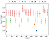 |
Fig. 22. Mean and standard deviation of the quiescent luminosity over the 10 binary orbits leading up to an outburst for different mass transfer rates. Mass transfer rates are given in units of 10−10 M⊙/yr. |
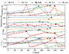 |
Fig. 23. Outburst duration, quiescent duration and visual magnitude, and the disk radius at the time of the maximum luminosity for different mass transfer rates. The mass transfer rates are given in units of 10−10 M⊙/yr. |
The averaged quiescence duration for each simulation follows the  relation from Osaki (1995). For the lowest mass transfer rate of 0.5 · 10−10 M⊙/yr, the quiescent duration becomes long for the outbursts to switch to inside-out (indicated by crosses instead of dots in Fig. 23). Overall, the transfer rate has no effect on the duration of the normal- or superoutbursts with the one exception being the inside-out outburst of the low transfer model.
Due to the weaker outbursts, the higher mass transfer simulations require more outbursts to reach the 3:1 radius, but do so in less time due to the significantly shorter accumulation timescale. We find no change in disk precession rate during a superoutburst with mass transfer rate and no change in the average superhump amplitude. However, the variability of the superhump amplitudes does increase with increasing mass transfer rate.
5.3. Mass ratio
Fig. 24 shows the outburst characteristics for different binary mass ratios q. Changing the mass ratio has similar characteristics in many cases to changing the mass transfer rates discussed in the previous section. Higher mass ratios result in smaller and more compact disks. The energy dissipation in the hot spot depends on the mass transfer rate and the relative velocity between the edge of the disk and the mass stream, which in turn depends on the disk size (Smak 2002). Consequently, we find brighter hot spots for smaller disk radii. During quiescence, the hot spot is the dominant luminosity source of the disk, so smaller disks will have higher quiescence luminosities. For the fiducial model, we find that the hot spot is 2.7 times brighter than the rest of the disk. We estimated this by comparing the quiescent luminosity with the luminosity of the disk after the mass transfer is turned off (see Fig. 18).
In addition, the conditions for an outburst are more easily met and the outburst frequency is increased. The more frequent outbursts lead to lower total disk masses, resulting in overall weaker outbursts. The increasing quiescent luminosity and decreasing outburst luminosity for higher mass ratios lead to the reduced visual magnitudes shown in the third panel of Fig. 24. The normal outburst durations have lower minima for higher mass ratios (compare the second cycle in the first panel of Fig. 24). However, we do not find a clear trend in the superoutburst durations, and our simulations did not run long enough to observe a trend in the supercycle duration.
For the higher mass ratios (and also for the higher mass transfer rate), the outer density ring is constantly at the critical temperature for an outburst (mid-plane temperatures of Tmid ≈ 9000 K). The simulations often launch weak heating waves that dissipate without leaving the density ring and without making the jump to ≈50 ⋅ 103 K observed in successful outbursts. These conditions are highlighted in Fig. 25, which shows the radial density profile and luminosity for each ring for the lowest and highest mass ratio simulations.
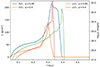 |
Fig. 25. Snapshots of the radial profiles of the surface density Σ and the disk luminosity L at radius r just before a superoutburst. |
The constant critical temperature in the outer density ring can be seen in the q = 0.4 simulation by the rise in luminosity inside the density ring, which does not occur in the q = 0.08 simulation. The plot also shows that the inner disk is colder for higher mass ratios and that the majority of the luminosity originates at the outer edge of the disk, outside of the density ring.
Simulations with mass ratios of q = 0.3 and higher produce reflares at the end of or just after superoutbursts. An example of these is shown in the first panel of Fig. 26. The first panel in Fig. 27 shows the reflares observed for V3101 Cyg for comparison. We explain these reflares with the increase in density in the inner parts of the disk due to the eccentricity dissipation observed in Fig. 7. As mentioned above, at these mass ratios, the outer density ring is constantly at the critical temperature and launches heating waves that can now propagate into the disk due to the increased density. Alternatively, these reflares have been explained by a mass transfer instability where the mass transfer is increased by several orders of magnitude (Hameury & Lasota 2021).
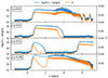 |
Fig. 26. Time evolution of the disk luminosities and the mass-weighted average of the aspect ratio for specific outbursts. |
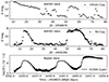 |
Fig. 27. Observed time evolution of luminosities for comparison with Fig. 26. The AAVSO data has been binned with a bin size of three times the cadence time to reduce noise. |
In our simulations, the superhump amplitudes increase with mass ratio (see Table 2). Since our superhump amplitudes for simulations with constant mass transfer rates are enhanced by narrow peaks not found in the observations, we see no value in evaluating the magnitudes further than the noted trend.
As can be seen in Table 2, the delay from precursor to superhumps and the superhump excess (or equivalently, the disk precession rate) increase with the binary mass ratio. Our superhump excess scales with the mass ratio as e(q) = 0.43 ⋅ q − 0.28 ⋅ q2, these values are about only half of the observed excess, which also has a different scaling: eobs(q) = 0.18 ⋅ q + 0.29 ⋅ q2 (Patterson et al. 2005). Our results are similar to the 2D SPH simulations of Smith et al. (2007). In this study they also performed 3D simulations that are in better agreement with observations. We also ran simulations with other cooling functions that resulted in cooler disks (cf. Fig. 6), but still found precession rates that were too low. Thus, the fact that our disks precess too slowly is probably due to the dimensionality of the simulations.
5.4. Mass ratio period gap
Observations find a period gap at Pbin = 2.8 h, which can be translated to a critical mass ratio of qcrit ≈ 0.3 (Inight et al. 2023) Systems with higher mass ratios typically do not produce superhumps. Although there are a few known exceptions (Hameury 2020, Sect. 4.7).
In our simulations, we found superoutbursts and superhumps for all mass ratios from q = 0.08 to 0.4, and each outburst evolved the same way, by first exceeding the 3:1 resonance radius, then filling out the Roche lobe and becoming eccentric, as shown in Fig. 1. These results are consistent with the 2D simulations in Smith et al. (2007), which found superhumps over an even wider range of mass ratios, but they also found a critical mass ratio of qcrit ≈ 0.24 for their 3D simulations above which no superhumps appeared. However, we do find that the time from the precursor outburst to the development of superhumps increases with the mass ratio (Table 2).
At high mass ratios, failed superoutbursts start to appear, which look like a precursor outburst to a superoutburst, but then launch a cooling wave instead of starting eccentricity growth. The light curve of a failed superoutburst is shown in the second panel of Fig. 26, the outburst has the same shape as the precursor of the superoutburst in the top panel. These outbursts could be interpreted as wide outbursts in systems above the period gap such as SS Cygni (see the second panel in Fig. 27). Buat-Ménard et al. (2001) explains these outbursts by an increase in tidal dissipation delaying the cooling wave. We argue that the tidal torques that stop the disk expansion and thus prevent further cooling by disk thinning are the more important effects in delaying the launching of the cooling wave. The delayed cooling wave gives these outbursts a flat top in the aspect ratio, which is different from the peak in the aspect ratio is seen in the normal outburst in the panel below, where the cooling wave is launched while the luminosity is still increasing.
The superoutburst in our q = 0.08 simulation behaves the opposite, it starts as a normal outburst as indicated by the shape of the aspect ratio curve in the fourth panel of Fig. 26, but as the cooling wave is moves inward, the eccentricity starts to grow and the tidal instability becomes active. This sequence of events is the same as described in Osaki & Kato (2014) for the observations of delayed superoutbursts in the CVs V1504 Cygni and V344 Lyrae. The third panel in Fig. 27 presents such a delayed superoutburst observed in V1504 Cygni. In our case, however, the cooling wave is only halfway through the disk when the tidal instability is launched, so that precursor and superoutburst are not separated in luminosity.
The low mass ratio simulations develop a superoutburst after the launch of the cooling wave, and the high mass ratio simulations do not develop a superoutburst even after staying in the outburst state for 2 days, indicating that it becomes more difficult to launch a superoutburst with an increasing mass ratio even in 2D.
6. Discussion and summary
In this study, we have performed 2D non-isothermal hydrodynamic simulations of outburst cycles in cataclysmic variable (CV) systems. Previous 2D simulations of CVs have used a locally isothermal equation of state (Smith et al. 2007; Wood & Burke 2007; Kley et al. 2008; Montgomery 2009) and could only study either the quiescent state or the outburst state. On the other hand, more realistic 3D simulations of full outburst cycles are not yet computationally feasible (Oyang 2022). While sophisticated 1D simulations of outburst cycles exist, see Hameury (2020) for a review, they cannot model the effects of disk eccentricity and have to approximate the gravitational torques acting on the disk.
We used a modified version of the FARGO code (Masset 2000) and added a non-perfect ideal equation of state (EoS) from Vaidya et al. (2015) that takes into account hydrogen ionization and dissociation. The gas was heated by viscous heating using the α parameter scaling from Ichikawa et al. (1993) and shock heating from Stone & Norman (1992, Appendix B). We used the cooling function from Ichikawa & Osaki (1992) which was developed to reproduce the S-shaped equilibrium curve during CVs outbursts. The momentum advection and compressive heating were not changed and are described in Rometsch et al. (2024)2.
Using this model and feeding the disk with a mass stream, we were able to self-consistently produce outburst cycles with normal outbursts and superoutbursts. We chose the parameters for our fiducial model so that the cycle duration and the number of normal outbursts in a cycle were consistent with observations of the V1504 Cygni system. From there, we performed a parameter study by changing a single parameter at a time. Our results are in agreement with the predictions of the thermal tidal instability model of Osaki (1989).
The αcold affects the luminosity and the diffusion timescale in the quiescent state while the mass transfer rate affects the accumulation timescale and the tidal energy dissipation in the hotspot. As described in Lasota (2001, Sect. 4.4), if the diffusion timescale is shorter than the accumulation timescale, outbursts are launched inside-out, otherwise they are launched outside-in. The variable mass transfer function, which scales the mass transfer rate with the accreted mass by Hameury et al. (2000), prolongs the superoutburst and improves the overall similarity to observed superoutbursts. The αhot parameter affects the energy dissipation during outbursts and their timescales. For the cooling function from Ichikawa & Osaki (1992), the value of the αhot parameter should be close to 0.1, higher values produce normal outburst durations that are shorter than observed.
The mass ratio of the binary determines the gravitational forces acting on the disk and thus affects the disk radius. For larger disk radii, caused by lower mass ratios, the model requires higher densities to trigger an outburst (Ichikawa & Osaki 1992). If the mass transfer rate is unchanged, this leads to longer quiescent phases, which is in agreement with observations of SU UMa systems (Menou 2000). The balance between gravitational and pressure forces also determines the precession rate of the disk (Goodchild & Ogilvie 2006), which we interpret as the superhump excess. We find faster precession and higher superhump excess for higher mass ratios, although our mass ratio to superhump excess scaling is too weak compared to the observations (Patterson et al. 2005) and it seems that 3D simulations are needed to get better agreement (Smith et al. 2007).
We also find higher superhump amplitudes for higher mass ratios. This trend seems to be opposite to observations that find higher amplitudes for longer binary orbital periods (lower mass ratios) (Kato et al. 2012, Sect. 4.7.1). In addition, there are several other caveats to our model.
In our model, the disk expands due to the enhanced angular momentum transfer during an outburst and contracts during the quiescent phase due to accreting low angular momentum gas from the donor star. Overall, the disk radius and mass increase with time. The conditions required to start an outburst in the model of Ichikawa & Osaki (1992) require higher densities at larger radii. For our constant mass transfer, it will therefore take more time to reach the critical densities at larger radii, and these higher densities will cause more viscous heating, leading to higher luminosities. While the monotonically increasing outburst luminosity is found in observations of V1504 Cygni (Cannizzo et al. 2012), the observed quiescent durations do not show clear trends. This could be introduced in simulations with non-constant mass transfer rates, but the exact physics behind the mass transfer rate is currently poorly understood. The luminosity increase for the first normal outburst after a superoutburst was not looked at in Cannizzo et al. (2012), but it also cannot be confirmed from their light curves.
Our simulations also produce outburst magnitudes that are too large, caused by the cooling model we took from Ichikawa & Osaki (1992) and used outside its intended purpose. We used this cooling function because the surface cooling with the Lin & Papaloizou (1985) opacity we used before required a too low temperature threshold ≈3000 K for the viscosity switch to produce outburst cycles, and it tended not to return to quiescence after a superoutburst if the mass transfer rate was too high. The effects of the different cooling functions are shown in Fig. 6, the model using the Lin & Papaloizou (1985) opacity has only half the mass transfer rate of the other models.
We also tested the cooling prescription by Kimura et al. (2020) (yellow line in Fig. 6), which is a revised version of the Ichikawa & Osaki (1992) cooling function with more efficient cooling on the hot branch. It produces a colder but still too hot outburst state and causes reflares where there were none for the fiducial model.
Opacity-based cooling leads to lower mid-plane temperatures during outbursts, which increases their duration due to the lower viscosity (compare the orange line in Fig. 6). The lower outburst temperatures increase the superhump excess from 1.8% to 2.1% for the variable mass transfer model, which is still well below the observed excess of 3.7%. Lower mid-plane temperatures would also make tidal dissipation heating more relevant, so that the superoutburst would be brighter compared to the precursor outburst, as is the case in observations. The same effect would also increase the superhump magnitudes, which is necessary since they are expected to be reduced by a factor of 2–4 when 3D effects are included (Smak 2009b).
The heating and cooling prescriptions in our model do not seem to be appropriate for the hot spot, and we found average hot spot temperatures that are a factor of three higher, with spontaneous peaks up to a factor of seven higher, than temperatures estimated from observations by Wood et al. (1989). Despite the excessively high temperatures, the total energy emitted by the hot spot is half of the value of theoretical estimates, see Sect. 4.3.4.
The amplitude of the flickering in the light curve caused by the hot spot is compatible with the amplitude found in observations, see Fig. 5. However, it should be noted that the flickering amplitude in our simulations depends on the mass transfer rate (Fig. 22), the cooling prescription (Fig. 6), and we find that it also scales with the numerical timestep size. There are several potential sources of flickering (Bruch 2021) of which only the hot spot is included in our model. Therefore, the flickering caused by the hotspot is overestimated in our simulations and the agreement with the observations seems to be a coincidence.
The model also predicts a monotonically increasing quiescent luminosity where observations find constant to decreasing luminosities. In our model, the quiescent luminosity increases due to the increasing viscous dissipation with increasing disk mass as well as the increasing tidal dissipation in the hot spot due to the shrinking disk radius. Our model therefore fails to explain the observed quiescence luminosities.
There are several 3D effects that we cannot model in 2D, but that are important for outburst behavior, such as eccentricity damping by vertical pressure forces (Oyang 2022, Chapter 4) or tilted disks that can explain negative superhump excess (Wood & Burke 2007; Montgomery 2009, 2012a,b). A three-dimensional mass stream could also overflow and underflow the disk, depositing its mass at different radii, see Godon (2019) for a recent study on this topic. This effect would change the evolution during quiescence (Kunze et al. 2001), the outbursts themselves (Schreiber & Hessman 1998), and the outburst recurrence rate (Kimura et al. 2020).
Nevertheless, our 2D simulations model the gravitational torques and allow us to study the effects of disk eccentricity on the outbursts. The main results of our study are the high superhump amplitudes we find in our simulation, the lack thereof in previous simulations is used as a criticism of the TTI model in Smak (2009b). We find gravitational torques during superoutbursts that are enhanced by almost two orders of magnitude (see Fig. 10) compared to the quiescent torques, which is higher than other studies assumed (cf. Sect. 5.3 Hameury 2020). Our model can reproduce complex outburst mechanisms such as delayed outbursts, long normal outbursts, and reflares at the end of superoutbursts, see Fig. 26, which we think should give credence to the TTI model of Osaki (1989).
Acknowledgments
This paper is dedicated to our friend and mentor Wilhelm Kley who introduced us to this topic. The authors acknowledge support from the High Performance and Cloud Computing Group at the Zentrum für Datenverarbeitung of the University of Tübingen, the state of Baden-Württemberg through bwHPC and the German Research Foundation (DFG) through grant no INST 37/935-1 FUGG. RK acknowledges financial support via the Heisenberg Research Grant funded by the German Research Foundation (DFG) under grant no. KU 2849/9. We acknowledge with thanks the variable star observations from the AAVSO International Database contributed by observers worldwide and used in this research.
References
- Astropy Collaboration (Price-Whelan, A. M., et al.) 2022, ApJ, 935, 167 [NASA ADS] [CrossRef] [Google Scholar]
- Bąkowska, K., & Olech, A. 2015, Acta Astron., 65, 351 [Google Scholar]
- Balbus, S. A., & Hawley, J. F. 1991, ApJ, 376, 214 [Google Scholar]
- Baruteau, C. 2008, Ph.D. Thesis, Observatoire de Paris [Google Scholar]
- Boley, A. C., & Durisen, R. H. 2006, ApJ, 641, 534 [Google Scholar]
- Bruch, A. 1996, A&A, 312, 97 [NASA ADS] [Google Scholar]
- Bruch, A. 2021, MNRAS, 503, 953 [NASA ADS] [CrossRef] [Google Scholar]
- Bruch, A., Beele, D., & Baptista, R. 1996, A&A, 306, 151 [NASA ADS] [Google Scholar]
- Buat-Ménard, V., Hameury, J. M., & Lasota, J. P. 2001, A&A, 366, 612 [NASA ADS] [CrossRef] [EDP Sciences] [Google Scholar]
- Cambier, H. 2015, MNRAS, 452, 3620 [NASA ADS] [CrossRef] [Google Scholar]
- Cannizzo, J. K., Smale, A. P., Wood, M. A., Still, M. D., & Howell, S. B. 2012, ApJ, 747, 117 [NASA ADS] [CrossRef] [Google Scholar]
- Chandrasekhar, S. 1960, Proc. Nat. Acad. Sci., 46, 253 [CrossRef] [Google Scholar]
- Coleman, M. S. B., Kotko, I., Blaes, O., Lasota, J. P., & Hirose, S. 2016, MNRAS, 462, 3710 [NASA ADS] [CrossRef] [Google Scholar]
- Cox, A. N., & Stewart, J. N. 1969, Nauchnye Informatsii, 15, 1 [NASA ADS] [Google Scholar]
- Coyne, R., Shenoy, A., MacLachlan, G., et al. 2012, ArXiv e-prints [arXiv:1206.6762] [Google Scholar]
- de Val-Borro, M., Edgar, R. G., Artymowicz, P., et al. 2006, MNRAS, 370, 529 [Google Scholar]
- Dubus, G., Otulakowska-Hypka, M., & Lasota, J.-P. 2018, A&A, 617, A26 [NASA ADS] [CrossRef] [EDP Sciences] [Google Scholar]
- Echevarría, J., Ramírez, S. H., Fuentes, M., et al. 2023, Rev. Mex. Astron. Astrofis., 59, 191 [Google Scholar]
- Eggleton, P. P. 1983, ApJ, 268, 368 [Google Scholar]
- Godon, P. 1996, MNRAS, 282, 1107 [NASA ADS] [CrossRef] [Google Scholar]
- Godon, P. 2019, ApJ, 870, 112 [NASA ADS] [CrossRef] [Google Scholar]
- Goodchild, S., & Ogilvie, G. 2006, MNRAS, 368, 1123 [NASA ADS] [CrossRef] [Google Scholar]
- Günther, R., Schäfer, C., & Kley, W. 2004, A&A, 423, 559 [NASA ADS] [CrossRef] [EDP Sciences] [Google Scholar]
- Hameury, J. M. 2020, Adv. Space Res., 66, 1004 [Google Scholar]
- Hameury, J. M., & Lasota, J. P. 2017, A&A, 602, A102 [Google Scholar]
- Hameury, J. M., & Lasota, J. P. 2021, A&A, 650, A114 [NASA ADS] [CrossRef] [EDP Sciences] [Google Scholar]
- Hameury, J.-M., Menou, K., Dubus, G., Lasota, J.-P., & Hure, J.-M. 1998, MNRAS, 298, 1048 [Google Scholar]
- Hameury, J.-M., Lasota, J.-P., & Warner, B. 2000, A&A, 353, 244 [NASA ADS] [Google Scholar]
- Hirose, S., Blaes, O., Krolik, J. H., Coleman, M. S. B., & Sano, T. 2014, ApJ, 787, 1 [NASA ADS] [CrossRef] [Google Scholar]
- Hubeny, I. 1990, ApJ, 351, 632 [NASA ADS] [CrossRef] [Google Scholar]
- Ichikawa, S., & Osaki, Y. 1992, PASJ, 44, 15 [NASA ADS] [Google Scholar]
- Ichikawa, S., Hirose, M., & Osaki, Y. 1993, PASJ, 45, 243 [NASA ADS] [Google Scholar]
- Inight, K., Gänsicke, B. T., Breedt, E., et al. 2023, MNRAS, 524, 4867 [NASA ADS] [CrossRef] [Google Scholar]
- Jordan, L. M., Kley, W., Picogna, G., & Marzari, F. 2021, A&A, 654, A54 [NASA ADS] [CrossRef] [EDP Sciences] [Google Scholar]
- Ju, W., Stone, J. M., & Zhu, Z. 2017, ApJ, 841, 29 [NASA ADS] [CrossRef] [Google Scholar]
- Kato, T., Maehara, H., Miller, I., et al. 2012, PASJ, 64, 21 [NASA ADS] [Google Scholar]
- Kimura, M., Osaki, Y., Kato, T., & Mineshige, S. 2020, PASJ, 72, 22 [NASA ADS] [CrossRef] [Google Scholar]
- King, A. R. 1988, QJRAS, 29, 1 [NASA ADS] [Google Scholar]
- Kley, W., Papaloizou, J. C. B., & Ogilvie, G. I. 2008, A&A, 487, 671 [NASA ADS] [CrossRef] [EDP Sciences] [Google Scholar]
- Kotko, I., & Lasota, J. P. 2012, A&A, 545, A115 [NASA ADS] [CrossRef] [EDP Sciences] [Google Scholar]
- Kunze, S., Speith, R., & Hessman, F. V. 2001, MNRAS, 322, 499 [NASA ADS] [CrossRef] [Google Scholar]
- Landstreet, J. D., Bagnulo, S., Martin, A., & Valyavin, G. 2016, A&A, 591, A80 [NASA ADS] [CrossRef] [EDP Sciences] [Google Scholar]
- Lasota, J.-P. 2001, New Astron Rev., 45, 449 [NASA ADS] [CrossRef] [Google Scholar]
- Lasota, J. P., Dubus, G., & Kruk, K. 2008, A&A, 486, 523 [NASA ADS] [CrossRef] [EDP Sciences] [Google Scholar]
- Latter, H. N., & Ogilvie, G. I. 2006, MNRAS, 372, 1829 [NASA ADS] [CrossRef] [Google Scholar]
- Lightkurve Collaboration (Cardoso, J. V. d. M., et al.) 2018, Astrophysics Source Code Library [record ascl:1812.013] [Google Scholar]
- Lin, D. N. C., & Papaloizou, J. 1985, in Protostars and Planets II, eds. D. C. Black, & M. S. Matthews, 981 [Google Scholar]
- Lubow, S. H. 1991, ApJ, 381, 259 [Google Scholar]
- Lubow, S. H., & Shu, F. H. 1975, ApJ, 198, 383 [NASA ADS] [CrossRef] [Google Scholar]
- Marzari, F., Baruteau, C., Scholl, H., & Thebault, P. 2012, A&A, 539, A98 [NASA ADS] [CrossRef] [EDP Sciences] [Google Scholar]
- Masset, F. 2000, A&AS, 141, 165 [NASA ADS] [CrossRef] [EDP Sciences] [Google Scholar]
- Mathew, A., & Nandy, M. K. 2017, RAA, 17, 061 [NASA ADS] [Google Scholar]
- McAllister, M. J., Littlefair, S. P., Baraffe, I., et al. 2015, MNRAS, 451, 114 [CrossRef] [Google Scholar]
- McAllister, M., Littlefair, S. P., Parsons, S. G., et al. 2019, MNRAS, 486, 5535 [NASA ADS] [CrossRef] [Google Scholar]
- Menou, K. 2000, Science, 288, 2022 [NASA ADS] [CrossRef] [Google Scholar]
- Meyer, F., & Meyer-Hofmeister, E. 1981, A&A, 104, L10 [NASA ADS] [Google Scholar]
- Mineshige, S., & Osaki, Y. 1983, PASJ, 35, 377 [NASA ADS] [Google Scholar]
- Mineshige, S., & Wood, J. H. 1989, MNRAS, 241, 259 [NASA ADS] [Google Scholar]
- Miranda, R., Muñoz, D. J., & Lai, D. 2017, MNRAS, 466, 1170 [NASA ADS] [CrossRef] [Google Scholar]
- Montgomery, M. M. 2009, MNRAS, 394, 1897 [NASA ADS] [CrossRef] [Google Scholar]
- Montgomery, M. M. 2012a, ApJ, 745, L25 [NASA ADS] [CrossRef] [Google Scholar]
- Montgomery, M. M. 2012b, ApJ, 753, L27 [NASA ADS] [CrossRef] [Google Scholar]
- Müller, T. W. A., Kley, W., & Meru, F. 2012, A&A, 541, A123 [NASA ADS] [CrossRef] [EDP Sciences] [Google Scholar]
- Nixon, C. J., Pringle, C. C. T., & Pringle, J. E. 2024, J. Plasma Phys., 90, 905900101 [NASA ADS] [CrossRef] [Google Scholar]
- Osaki, Y. 1989, PASJ, 41, 1005 [NASA ADS] [Google Scholar]
- Osaki, Y. 1995, PASJ, 47, 47 [NASA ADS] [Google Scholar]
- Osaki, Y., & Kato, T. 2014, PASJ, 66, 15 [NASA ADS] [CrossRef] [Google Scholar]
- Osaki, Y., & Meyer, F. 2004, A&A, 428, L17 [NASA ADS] [CrossRef] [EDP Sciences] [Google Scholar]
- Oyang, B. 2022, Ph.D. Thesis, University of California, Santa Barbara, USA [Google Scholar]
- Oyang, B., Jiang, Y.-F., & Blaes, O. 2021, MNRAS, 505, 1 [NASA ADS] [CrossRef] [Google Scholar]
- Pala, A., Gänsicke, B., Belloni, D., et al. 2022, MNRAS, 510, 6110 [NASA ADS] [CrossRef] [Google Scholar]
- Patterson, J., Kemp, J., Harvey, D. A., et al. 2005, PASP, 117, 1204 [Google Scholar]
- Picogna, G., & Marzari, F. 2013, A&A, 556, A148 [NASA ADS] [CrossRef] [EDP Sciences] [Google Scholar]
- Pjanka, P., & Stone, J. M. 2020, ApJ, 904, 90 [NASA ADS] [CrossRef] [Google Scholar]
- Pratt, G. W., Hassall, B. J. M., Naylor, T., Wood, J. H., & Patterson, J. 1999, MNRAS, 309, 847 [NASA ADS] [CrossRef] [Google Scholar]
- Rolfe, D. J., Haswell, C. A., & Patterson, J. 2001, MNRAS, 324, 529 [CrossRef] [Google Scholar]
- Rometsch, T., Jordan, L. M., Moldenhauer, T. W., et al. 2024, A&A, 684, A192 [NASA ADS] [CrossRef] [EDP Sciences] [Google Scholar]
- Scepi, N., Lesur, G., Dubus, G., & Flock, M. 2018, A&A, 609, A77 [NASA ADS] [CrossRef] [EDP Sciences] [Google Scholar]
- Scepi, N., Dubus, G., & Lesur, G. 2019, A&A, 626, A116 [NASA ADS] [CrossRef] [EDP Sciences] [Google Scholar]
- Schreiber, M. R., & Hessman, F. V. 1998, MNRAS, 301, 626 [CrossRef] [Google Scholar]
- Schreiber, M. R., Belloni, D., & Schwope, A. D. 2024, A&A, 682, L7 [NASA ADS] [CrossRef] [EDP Sciences] [Google Scholar]
- Shakura, N. I., & Sunyaev, R. A. 1973, A&A, 24, 337 [NASA ADS] [Google Scholar]
- Smak, J. 1984, Acta Astron., 34, 161 [NASA ADS] [Google Scholar]
- Smak, J. 1995, Acta Astron., 45, 355 [NASA ADS] [Google Scholar]
- Smak, J. 2002, Acta Astron., 52, 263 [NASA ADS] [Google Scholar]
- Smak, J. 2009a, Acta Astron., 59, 121 [NASA ADS] [Google Scholar]
- Smak, J. 2009b, Acta Astron., 59, 103 [NASA ADS] [Google Scholar]
- Smak, J., & Waagen, E. O. 2004, Acta Astron., 54, 433 [NASA ADS] [CrossRef] [Google Scholar]
- Smith, A. J., Haswell, C. A., Murray, J. R., Truss, M. R., & Foulkes, S. B. 2007, MNRAS, 378, 785 [NASA ADS] [CrossRef] [Google Scholar]
- Stone, J. M., & Norman, M. L. 1992, ApJS, 80, 753 [Google Scholar]
- Tetarenko, B. E., Lasota, J. P., Heinke, C. O., Dubus, G., & Sivakoff, G. R. 2018, Nature, 554, 69 [Google Scholar]
- Tscharnuter, W. M., & Winkler, K. H. A. 1979, Comput. Phys. Commun., 18, 171 [NASA ADS] [CrossRef] [Google Scholar]
- Vaidya, B., Mignone, A., Bodo, G., & Massaglia, S. 2015, A&A, 580, A110 [NASA ADS] [CrossRef] [EDP Sciences] [Google Scholar]
- Velikhov, E. P. 1959, Sov. J. Exp. Theor. Phys., 9, 995 [NASA ADS] [Google Scholar]
- Viallet, M., & Hameury, J. M. 2008, A&A, 489, 699 [NASA ADS] [CrossRef] [EDP Sciences] [Google Scholar]
- Vogt, N. 1983, A&A, 128, 29 [NASA ADS] [Google Scholar]
- Warner, B. 2003, Cataclysmic Variable Stars (Cambridge, UK: Cambridge University Press) [Google Scholar]
- Whitehurst, R. 1988, MNRAS, 232, 35 [NASA ADS] [Google Scholar]
- Wood, M. A., & Burke, C. J. 2007, ApJ, 661, 1042 [NASA ADS] [CrossRef] [Google Scholar]
- Wood, J. H., Horne, K., Berriman, G., & Wade, R. A. 1989, ApJ, 341, 974 [NASA ADS] [CrossRef] [Google Scholar]
All Tables
All Figures
|
Fig. 1. Two-dimensional snapshots of the mid-plane temperature before and during a superoutburst for our fiducial setup, whose parameters are listed in Table 1. The cyan circle indicates the 3:1 resonance and the green line indicates the Roche lobe. The time in days is measured from the beginning of the outburst and one day is equal to 14.1 binary orbits (1.7 h). The simulation ran in a corotating reference frame, with the donor star fixed on the right side. |
| In the text | |
|
Fig. 2. Top panel: thermal equilibria [Teff] vs. [Σ] from the shearing box simulations in Scepi et al. (2018) (data taken from their Table 1) and the model from Ichikawa & Osaki (1992) for the same input parameters. Bottom panel: the measured α parameters in Scepi et al. (2018) and the interpolation function Eq. (6) as a function of the mid-plane temperature. |
| In the text | |
|
Fig. 3. Top panel: Disk eccentricity evolution for locally isothermal models with different boundary conditions. Bottom panel: Time evolution of the longitude of pericenter of the disk in radians. |
| In the text | |
|
Fig. 4. Radial profiles of mass-weighted azimuthally averaged disk eccentricity and azimuthally averaged surface density. All profiles were also averaged over 20 simulation snapshots from simulation times 140 to 160 binary periods. |
| In the text | |
|
Fig. 5. The upper panels show Kepler data of V1504 Cygni over an equal length time frame as the simulated data below. The binary period is 1.7 hours, and one day is equal to 14.1 binary periods. The extent of the y-axis in the left panel is the same as in the plot below, but in the right panel, the extent of the y-axis is reduced by a factor of 3.8 compared to the plot below. Bottom left panel: Luminosity, disk radius, eccentricity, and total mass as a function of time for the fiducial model. The orange line indicates the 3:1 orbital resonance radius. The red dashed line indicates the time at which the right panel is zoomed in and the black dashed line indicates the start of the second superoutburst. Bottom right panel: Zoom in on the same quantities during a superoutburst as a function of the longitude of pericenter of the disk relative to the position of the binary. The angles are shifted by π and normalized so that integer values indicate that the binary passes the bulge of the eccentric disk. |
| In the text | |
|
Fig. 6. Comparison of the luminosity curves for the fiducial model using the cooling prescription from Ichikawa & Osaki (1992) (blue line), the revised version of that cooling prescription from Kimura et al. (2020) (yellow line) and a model using surface cooling with opacities from (Lin & Papaloizou 1985) (orange line) as well as Kepler data of V1504 Cygni (black line). |
| In the text | |
|
Fig. 7. Azimuthally averaged density distributions as a function of radius before (1, 2) and after (1′ and 2′) the first and second normal outbursts following a superoutburst. The solid lines are taken from the first and the dashed lines from the second supercycle of the fiducial model. |
| In the text | |
|
Fig. 8. Luminosity and disk radius evolution during a normal, outside-in outburst of our fiducial model (αcold = 0.02) and an inside-out outburst of our αcold = 0.04 model. Squares and dots indicate what we define as the start of the outburst, the start of the heating wave, the peak, and the end of the outburst. |
| In the text | |
|
Fig. 9. Kepler luminosity data during two consecutive outbursts of V344 Lyr for comparison with Fig. 8. |
| In the text | |
|
Fig. 10. Azimuthal and time-averaged (over 10 Pbin) gravitational torque density Eq. (16) during different stages of a superoutburst. The vertical dashed lines are the time-averaged disk radii during the same time frame. The black vertical line indicates the position of the 3:1 resonance. The legend also notes the total integrated torques exerted on the disk, normalized to the torque during quiescence. |
| In the text | |
|
Fig. 11. Evolution of several quantities during a superoutburst for our fiducial model (blue) and variable mass transfer model using Eq. (24) (orange). The solid lines represent the disk luminosity while the dots and squares indicate the timestamps of the start, the peak, and the end of the outburst. Also shown are the mass-weighted disk eccentricity (dashed line) and the disk mass (dash-dotted line). |
| In the text | |
|
Fig. 12. Luminosity evolution during a superoutburst for our variable mass transfer model (orange line, same as in Fig. 11) and Kepler data of V1504 Cygni (black line). The shaded regions indicate the time frames presented in Fig. 14. The orange dashed line is the torque exerted by the disk on the donor star. No units are given for the torque because we are only making a qualitative assessment. |
| In the text | |
|
Fig. 13. Superhump amplitudes for the variable mass transfer model and V1504 Cygni measured from the data presented in Fig. 12. |
| In the text | |
|
Fig. 14. Luminosity of the variable mass transfer model and Kepler data of V1504 Cygni during different phases of the superoutburst as indicated in Fig. 12. The time is measured from the start of the superoutburst. The crosses indicate the minima and maxima of the superhumps used in further evaluation. |
| In the text | |
|
Fig. 15. The disk precession rate during a superoutburst, together with the torque exerted by the disk on the donor star and the negative of the gas aspect ratio squared. The luminosity curve in the background is for orientation only. |
| In the text | |
|
Fig. 16. Superhump excess calculated from adjacent peaks or minima for our variable mass transfer model (red or blue crosses, see the first panel in Fig. 14). The blue dots are an average of nearby data points and the orange dots are the precession rate of the disk. The black dots are the superhump excess computed from Kepler data of V1504 Cygni using an orbital period of 1.668 h (Coyne et al. 2012). |
| In the text | |
|
Fig. 17. Luminosity curves for the fiducial model during the high eccentricity phase of a superoutburst compared to a restart with the mass transfer turned off. |
| In the text | |
|
Fig. 18. Luminosities during the first normal outburst following a superoutburst. The black line presents Kepler data of V344 Lyr, the blue line is for our Ṁtr = 2.5 · 10−10 M⊙/yr model and the orange is a simulation of the same model but restarted with the mass transfer turned off. |
| In the text | |
|
Fig. 19. The visual magnitude, duration, and symmetry of the outbursts, and the quiescent duration between outbursts for different αhot parameters. |
| In the text | |
|
Fig. 20. Same as Fig. 19 but for Kepler data of V1504 Cyg. The two lines represent two different outburst cycles. |
| In the text | |
|
Fig. 21. Quiescent duration between outbursts for different αcold parameters. Dots indicate normal outbursts, crosses indicate inside-out normal outbursts, and squares indicate superoutbursts. |
| In the text | |
|
Fig. 22. Mean and standard deviation of the quiescent luminosity over the 10 binary orbits leading up to an outburst for different mass transfer rates. Mass transfer rates are given in units of 10−10 M⊙/yr. |
| In the text | |
|
Fig. 23. Outburst duration, quiescent duration and visual magnitude, and the disk radius at the time of the maximum luminosity for different mass transfer rates. The mass transfer rates are given in units of 10−10 M⊙/yr. |
| In the text | |
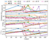 |
Fig. 24. Same as Fig. 23 but for different binary mass ratios q. |
| In the text | |
|
Fig. 25. Snapshots of the radial profiles of the surface density Σ and the disk luminosity L at radius r just before a superoutburst. |
| In the text | |
|
Fig. 26. Time evolution of the disk luminosities and the mass-weighted average of the aspect ratio for specific outbursts. |
| In the text | |
|
Fig. 27. Observed time evolution of luminosities for comparison with Fig. 26. The AAVSO data has been binned with a bin size of three times the cadence time to reduce noise. |
| In the text | |
Current usage metrics show cumulative count of Article Views (full-text article views including HTML views, PDF and ePub downloads, according to the available data) and Abstracts Views on Vision4Press platform.
Data correspond to usage on the plateform after 2015. The current usage metrics is available 48-96 hours after online publication and is updated daily on week days.
Initial download of the metrics may take a while.