| Issue |
A&A
Volume 692, December 2024
|
|
|---|---|---|
| Article Number | A41 | |
| Number of page(s) | 24 | |
| Section | Numerical methods and codes | |
| DOI | https://doi.org/10.1051/0004-6361/202450828 | |
| Published online | 03 December 2024 | |
Supervised machine learning on Galactic filaments
II. Encoding the position to optimize the detection of filaments over a wide range of column density and contrast
1
Aix Marseille Univ, CNRS, LIS,
Marseille,
France
2
Aix Marseille Univ, CNRS, CNES, LAM
Marseille,
France
3
Institut Universitaire de France,
1 rue Descartes,
75005
Paris,
France
4
INAF–IAPS,
Via Fosso del Cavaliere 100,
Rome,
Italy
5
National Astronomical Observatory of Japan,
Osawa 2-21-1, Mitaka,
Tokyo
181-8588,
Japan
★ Corresponding author; This email address is being protected from spambots. You need JavaScript enabled to view it.
Received:
22
May
2024
Accepted:
2
September
2024
Abstract
Context. Filaments host star formation and are fundamental structures of galaxies. Their diversity, as observed in the interstellar medium, from very low-density structures to very dense hubs, and their complex life cycles make their complete detection challenging over this large diversity range.
Aims. Using 2D H2 column density images obtained as part of the Herschel Hi-GAL survey of the Galactic plane (Gp), we want to detect, simultaneously and using a single model, filaments over a large range of column density and contrast over the whole Gp. In particular, we target low-contrast and low-density structures that are particularly difficult to detect with classical algorithms.
Methods. The whole H2 column density image of the Gp was subdivided into individual patches of 32 × 32 pixels. Following our proof of concept study aimed at exploring the potential of supervised learning for the detection of filaments, we propose an innovative supervised learning method based on adding information by encoding the position of these patches in the Gp. To allow the segmentation of the whole Gp, we introduced a random procedure that preserves the balance within the model training and testing datasets over the Gp plane. Four architectures and six models were tested and compared using different metrics.
Results. For the first time, a segmentation of the whole Gp has been obtained using supervised deep learning. A comparison of the models based on metrics and astrophysical results shows that one of the architectures (PE-UNet-Latent), where the position encoding was done in the latent space gives the best performance to detect filaments over the whole range of density and contrast observed in the Gp. A normalized map of the whole Gp was also produced and reveals the highly filamentary structure of the Gp in all density regimes. We successfully tested the generalization of our best model by applying it to the 2D 12CO COHRS molecular data obtained on a 58.°8 portion (in longitude) of the plane.
Conclusions. We demonstrate the interest of position encoding to allow the detection of filaments over the wide range of density and contrast observed in the Gp. The produced maps (both normalized and segmented) offer a unique opportunity for follow-up studies of the life cycle of Galactic filaments. The promising generalization possibility tested on a molecular dataset of the Gp opens new opportunities for systematic detection of filamentary structures in the big data context available for the Gp.
Key words: stars: formation / ISM: clouds / ISM: structure / infrared: ISM
© The Authors 2024
 Open Access article, published by EDP Sciences, under the terms of the Creative Commons Attribution License (https://creativecommons.org/licenses/by/4.0), which permits unrestricted use, distribution, and reproduction in any medium, provided the original work is properly cited.
This article is published in open access under the Subscribe to Open model. This email address is being protected from spambots. You need JavaScript enabled to view it. to support open access publication.
1 Introduction
The galactic interstellar medium (ISM) is structured in filamentary molecular clouds that span a large range of properties over a wide range of physical conditions (Dib et al. 2020; Soler et al. 2022; Feng et al. 2024; Schisano et al. 2020). As revealed by the results of the Herschel Gould Belt (André et al. 2010) and the Herschel infrared Galactic Plane Survey (Hi-GAL) (Molinari et al. 2010), the cold and warm ISM is organized in a ubiquitous network of filaments in which star formation is generally observed above a density threshold corresponding to AV = 7 mag (André et al. 2014; Könyves et al. 2020). Galactic filaments exhibit a large range of structures that depend on the spatial resolution and the tracers used to observe them (Hacar et al. 2023). They also present complex life cycles ranging from the low-density cold ISM to the high-density medium where stars form. During this life cycle, filaments are built from the diffuse ISM, fragment, and fuel material to allow star formation. All these phases of formation are widely studied in both observations and simulations to fully describe the star formation process (André et al. 2010; Molinari et al. 2010; Arzoumanian et al. 2011; Hacar et al. 2018; Arzoumanian et al. 2019; Shimajiri et al. 2019; Clarke et al. 2020; Priestley & Whitworth 2022; Hacar et al. 2023; Pillsworth & Pudritz 2024, and references therein). In particular, the way the filaments form and evolve in the ISM is still debated (Hoemann et al. 2021; Hsieh et al. 2021; Pineda et al. 2022; Feng et al. 2024). Part of this debate is linked to the role of high-mass stars (M⋆ ≥ 8 M⊙) that preferentially form at the junction of filaments called hubs (Kumar et al. 2020, 2022) and their associated ionized (H II) region that impact the structure of the surrounding medium, modifying the filament structure and the future star formation therein (Peretto et al. 2012; Zavagno et al. 2020; Maity et al. 2023; Bešlić et al. 2024).
Because filaments exhibit both a wide range of shapes and lengths and have a complex life-cycle (Pillsworth & Pudritz 2024), their global detection (using one method and the same set of parameters at the same time) over a wide range of densities and contrasts is needed to fully understand the star formation process. The key importance of detecting filaments over a wide range of densities to understand their life cycle in the ISM and the large quantity of data available on the Galactic plane (Gp) led to the natural development of many filament extraction algorithms used both for numerical simulations and for observational data. These methods can be divided into four main categories: Some approaches concentrate on a local examination of the structures, relying on local derivatives at the level of individual pixels. In contrast, alternative methods take a non-local approach, investigating a larger surrounding zone for each pixel to identify characteristic spatial scales that define the filament. The third category of techniques advocates for a comprehensive analysis of the entire map, employing decomposition at a multi-scale level. Lately, statistical methods supported by supervised machine learning have been proposed to extract filaments based on existing catalogues to overcome the issues stated above. Descriptions of methods within these four categories are given in Section 2.
While the first approaches are radically different, they share the common feature that a single setting of the parameters does not allow a complete filament extraction over the large range of density and contrast values observed in the data. A close visual inspection of 2D images and 3D (position, position, velocity) spectral data cubes shows that some filaments are not detected by state-of-the-art algorithms, especially low-contrast and/or low-density filaments. This means that it is very difficult, in particular for large surveys of the Gp, to deliver a complete catalogue that is as unbiased as possible of the filaments present in the data. Another limitation of these algorithms comes from their computation time, which can make some of them too expensive to envision a complete threshold and extraction parameter optimization. Because the multi-wavelength information available on the Gp on all spatial scales is so rich, proposing another way of extracting filaments might allow a leap forward for an unbiased census of filaments present in the data. Machine learning, through neural networks, is a new way to explore filament detection with no hyper-parameters, at low cost, given an already-established filament catalogue (supervised learning being the most widespread and simple learning strategy). Facing the difficulty of detecting filaments over the large range of column density (ranging from 1020 to 1023 cm−2) and contrast (column density ratio between filaments and background) observed in the Gp (Schisano et al. 2020), using a single model and a single set of parameters, we propose a novel approach that combines supervised deep learning with an innovative data distribution strategy. Capitalizing on our proof-of-concept study that explored the interest of supervised deep learning for the detection of filaments (Zavagno et al. 2023), we also use here the whole column density image of the Gp obtained from the Hi-GAL dataset (Molinari et al. 2016). As explained in Zavagno et al. (2023, Section 2.2), this image and its associated masks (all with an original size of 150 000 × 2000 pixels) are subdivided into individual patches of 32 × 32 pixels (the minimum size accepted by the UNet architecture and chosen to preserve the structure of the smallest filaments; see Zavagno et al. 2023, Section 2.2) that are randomly distributed along the longitude axis for the learning stage, using a random distribution procedure that we introduce here. Moreover, based on the observed distribution of the filaments in the Gp (Schisano et al. 2020), we propose a new UNet-based architecture called Position-Encoding-UNet (PE-UNet) that, adding the information about the position of the patch within the Gp, significantly improves the state-of-the-art detection of filaments. We tested several architectures and compare their performance using both machine learning metrics and their results on the detection of filaments using astrophysical data. We also explore the generalization capability of our best model and discuss its implication for the study of filaments in the Gp.
The structure of the paper is as follows. Section 2 gives an overview of filament detection methods, while Section 3 briefly presents the machine learning concepts used for this work. Section 4 introduces the Hi-GAL dataset used, Section 5 provides details about the random data distribution strategy employed for segmenting the entire Gp and introduces the position-encoding (PE-UNet) architecture. Section 6 describes our experimental settings (metrics, machine learning environment), Section 7 presents the results from the machine learning and the astrophysics standpoint, and are discussed in Section 8. The main results and perspective of this work are summarized in Section 9.
2 Overview of filament detection methods
Local techniques usually involve the computation of either the gradient (first-order derivatives) as demonstrated by Soler et al. (2013) and Planck Collaboration Int. XXXII (2016), or the Hessian matrix (second-order derivatives) as shown in works by Polychroni et al. (2013), Schisano et al. (2014), and Planck Collaboration Int. XXXII (2016) at each pixel. The goal of first-order derivatives is to determine the orientations of elongated structures from statistical analyses which will result in filaments, following the approaches of Soler et al. (2013) and Planck Collaboration Int. XXXII (2016). Alternatively, the method proposed by Schisano et al. (2014) is based on the thresholding of the eigenvalues of the Hessian matrix that leads to the identification of 2 D regions where the emission locally resembles a cylindrical filament. The method has been applied to Benedettini et al. (2015); Pezzuto et al. (2021); Fiorellino et al. (2021). Some methods focus on extracting filament skeletons by connecting adjacent pixels along the crests of the (intensity or column density) distribution. For example, the DisPerSe method, initially designed for recovering filament skeletons in cosmic web maps by Sousbie (2011), has been effectively applied to Herschel column density maps (Arzoumanian et al. 2011, 2019; Peretto et al. 2012; Palmeirim et al. 2013) and 13CO intensity maps (Panopoulou et al. 2014). Different from DisPerSe (Sousbie 2011), CRISPy (Chen et al. 2020) performs filament detection thanks to ridge estimation (Chen et al. 2014, 2015) and has been used to analyse the velocity structure of the long and high-mass star forming NGC 6334 filamentary cloud (Arzoumanian et al. 2022). A drawback of the local approach is its difficulty in detecting faint structures such as striations or low-contrast filaments.
The non-local category is mainly composed of templatematching algorithms (Juvela 2016) that search for one or several specific and user-defined morphologies building a probability map to find such a structure. Another effective approach is the Rolling Hough Transform (RHT) method by Clark et al. (2014), which calculates an estimator of the linearity level of structures in the vicinity of a pixel at a given scale, utilizing the Hough transform. This method has been extensively applied in various studies involving H I data, Herschel, and Planck maps (Clark et al. 2015; Clark & Hensley 2019; Malinen et al. 2016; Panopoulou et al. 2016; Alina et al. 2019). filfinder (Koch & Rosolowsky 2015) extracts filament skeletons by first performing spatial filtering at a specific scale, covering a dynamic range broad enough to encompass striations. Extending the RHT algorithm, Carrière et al. (2022b,a) proposed FilDReaMS which overcomes RHT limitations by discretizing the spatial space through a first pattern-matching step. The preferred orientation is then chosen by performing a local maxima search and comparing it to a random distribution rather than an arbitrary threshold as in RHT.
Global approaches provide a comprehensive analysis across multiple scales for a given field. The getfilaments technique, introduced by Men’shchikov (2013), employs statistical tools and morphological filtering to extract a filament network while mitigating background noise. It also identifies point sources and supports a multi-wavelength analysis. While this method is thorough, it necessitates fine-tuning and supplementary tools for extracting filament orientations and scales. It has been successfully applied to Herschel maps in studies by Cox et al. (2016); Rivera-Ingraham et al. (2016, 2017). Men’shchikov (2021) proposed an upgraded version of getfilaments, namely getsf which combines sources and filaments extraction for better results. Following Men’shchikov (2013), getsf performs source, filament and background separation simultaneously for better results (sources and filaments are closely related) based on multi-wavelength analysis. It has been successfully applied in Motte et al. (2022); Pouteau et al. (2022); Kumar et al. (2022); Xu et al. (2023b). Alternatively, Salji et al. (2015a,b) used the Frangi filter (Frangi et al. 1998) to JCMT continuum images to extract filaments. The Frangi filter is a method that allows multi-scale identification of filaments based on the detection of ridges and it adopts the analysis of the Hessian matrix. On the other hand, wavelet-based methods by Robitaille et al. (2019); Ossenkopf-Okada & Stepanov (2019) leverage an anisotropic wavelet analysis to extract an entire filament network by scrutinizing map fluctuations across spatial scales. This approach may overcome inherent biases associated with commonly used methods (Panopoulou et al. 2017) and remains relatively efficient. Nevertheless, additional steps are required to determine filament orientations. Despite its multi-scale nature, the log space scaling inherent in wavelet analysis results in decreased resolution at larger spatial scales.
Lastly, statistical methods, mainly based on machine learning, have been used in Alina et al. (2022); Zavagno et al. (2023); Xu et al. (2023a) showing promising results in terms of computation time and easier to tune than other existing methods. Both works used UNet-like (Ronneberger et al. 2015) architecture in a supervised manner to perform the filament mask extraction through the semantic segmentation task, where the goal is to classify each pixel of a given image with labels (Fu & Mui 1981, for a review).
3 Brief overview of machine learning concepts
In this section, we introduce the key concept of the machine learning approach used, centred around semantic segmentation. Semantic segmentation consists of associating one label (or category) with each pixel of an input image. It is a well-studied task in the computer vision field, with many applications, for instance in the medical domain (Thoma 2016; Huang et al. 2022; Asgari Taghanaki et al. 2021), to automatically detect organs or tumors in medical images and videos, and more recently in astrophysics with a few recent applications on galaxies such as presented in Zhu et al. (2019); Hausen & Robertson (2020); Bianco et al. (2021); Bekki (2021). Filament detection has also been addressed as a segmentation task in Schisano et al. (2014, Schisano et al. 2020); Clark et al. (2014); Carrière et al. (2022b,a); Alina et al. (2022); Zavagno et al. (2023) works with or without machine learning. Today, semantic segmentation is systematically tackled with deep learning models (Goodfellow et al. 2016), mainly with Convolution Neural Network (CNN) (LeCun et al. 1989; Krizhevsky et al. 2017; He et al. 2016) and most often with what is called UNet architectures (Ronneberger et al. 2015), the current state-of-the-art models for this task.
The UNet architecture is a neural network with an autoencoder-like structure, whose output has the same shape as its input and whose inner hidden layer is of much lower dimension than the input (see Figure 1). While an autoencoder is learnt to reconstruct its input at its output while going through a bottleneck (a compressed representation of its input which is computed in its hidden layer), a UNet is learnt to output the segmentation image of the input image. The UNet is a rather standard deep autoencoder (i.e. an autoencoder with many layers) that includes a series of convolution and pooling layers in the encoder, up to the most compressed representation of the input, and a series of convolution and transpose convolution layers in the decoder (see Figure 1). The specificity of UNet resides in skip connections that connect intermediate layers of the encoder to corresponding layers in the decoder. The skip connections allow multi-scale processing of the input and facilitate the flow of detailed spatial information from the encoding to the decoding stage, which facilitates precise localization and segmentation. The final layer of the UNet architecture usually consists of a 1 × 1 convolution.
Countless variations of UNet have been proposed for semantic segmentation, particularly within the medical domain. We mention only a few below. Attention UNets (Oktay et al. 2018) made use of attention mechanisms (Jetley et al. 2018) to selectively emphasize informative regions in the feature maps. By focusing on relevant features, attention UNet achieves better segmentation performance, especially in scenarios with complex backgrounds. Residual UNets were a rather straightforward extension of UNets (Zhang et al. 2018) exploiting residual connections as popularized in ResNets (He et al. 2016). This variant enhances gradient flow during training and facilitates the training of deeper networks, leading to improved segmentation accuracy. Besides, UNet3+ (Huang et al. 2020) extended the capabilities of the original UNet architecture by introducing the Full-Scale Connected path, hierarchical attention mechanisms, and multi-level feature fusion, thereby enhancing its performance in medical image segmentation tasks. This variant is particularly well suited for scenarios where precise delineation of structures and accurate localization of abnormalities are crucial, such as in medical diagnosis and treatment planning. Finally, DenseUNet (Bui et al. 2019) integrates dense blocks, as proposed in DenseNet architectures (Jégou et al. 2017), into the UNet framework, where dense blocks encourage feature reuse and facilitate gradient flow throughout the network, leading to improved segmentation performance.
In our work we chose to compare our PE-UNet (described in Section 5.2) to a few baselines: the standard and original UNet (Ronneberger et al. 2015) which remains a reference model for semantic segmentation; the UNet++ (Zhou et al. 2019) which constitutes the state-of-the-art architecture on the Hi-GAL column density (NH2) dataset (Zavagno et al. 2023) and the SwinUNet (Cao et al. 2023) which recently took over state-of-the-art performance in the image medical field. We briefly discuss the two latter models.
The UNet++ (Zhou et al. 2019) model is based on the original UNet architecture where skip connections have been replaced with a series of nested dense skip pathways to improve the multi-scale performance of the network, i.e. to better take into account details captured in high-resolution layers for the final segmentation. It usually performs well in the case of small objects.
Swin-UNet (Cao et al. 2023) combines the UNet architecture with the Swin Transformer block (Liu et al. 2021), it is the first fully transformer-based UNet. The Swin Transformer block is based on a shifted window multi-head self-attention module (replacing the traditional multi-head self-attention module) to gather context information between neighbouring patches. Transformers and self-attention layers have revolutionized the field of Natural Language Processing and spread to computer Vision (Dosovitskiy et al. 2020) and are a new powerful brick to build modern deep learning architectures. The Swin-UNet model is composed of a traditional encoder, a bottleneck, and a decoder, all of these are based on the Swin Transformer block (Liu et al. 2021). It achieves state-of-the-art performance on the Synapse dataset1.
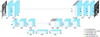 |
Fig. 1 Simplified UNet architecture (Ronneberger et al. 2015). The complete architecture is composed of 5 UNet blocks (here only three are represented). A UNet block is composed of two convolutions 3 × 3 and Relu activation followed by a max pooling layer for the encoding part and one up-convolution layer followed by two convolutions 3 × 3 and Relu activation for the decoding part. Skip connections correspond to the concatenation operation and are represented by dashed lines. With our implementation (five blocks), we obtain an output of size 2 × 2 × 1024 after the bottleneck given an image of size 32 × 32 × 1. The input image is represented on the left, while the output is shown on the right. |
4 Dataset
4.1 Data
The Hi-GAL survey of the Gp (Molinari et al. 2010) is a photometric survey performed by the Herschel Space Observatory (Pilbratt et al. 2010) in five photometric bands from 70 to 500 μm. After calibration, NH2 and dust temperature maps are computed from the photometric images. To obtain the NH2 and dust temperature maps, Herschel photometric data are convolved to the 500 μm resolution (36″) and a pixel-by-pixel fitting by a single temperature grey body is done (the complete pipeline description can be found in Elia et al. (2013) and Schisano et al. (2020)). It results in 37 mosaics, with an overlap over its two neighbours of ~2.2° (with a pixel size of 11.5″), covering the entirety of the Gp. When merging the mosaics all together with the reproject module from Astropy Collaboration (2022), the whole Gp image is contained in an image of 1800 × 114 000 pixels. Schisano et al. (2020) adopted simple criteria of thresholding the minimum eigenvalue identifying all the regions where there is a quick variation of the emission, then introduced selection criteria based on the shape of the extracted region to identify among all the features the one that resembles a filamentary morphology. Their work resulted in the publication of the first catalogue, composed of 32059 filaments over the entire Gp.
4.2 Labelling strategy
We rely on data which have been labelled by Schisano et al. (2020). From the beginning, we know that this labelling is not complete, as some filaments are not detected, hence, starting from a two-class labelling, there would exist pixels that are wrongly labelled as background. To avoid training our models on partially wrongly labelled data, drawing from the methodology outlined in the work of Zavagno et al. (2023), we classify pixels into three distinct categories: filament, background and unknown:
Filament pixels are pixels identified as such according to the list of filament published by Schisano et al. (2020).
Background pixels are defined through a hand-crafted thresholding method, mosaic by mosaic. We define a threshold on the column density value for each mosaic such that every pixel below the threshold is not with very high confidence a filament.
Pixels that do not fall into the two categories defined above are considered as unknown pixels, in, particular no supervision and model evaluation is done on these pixels.
When training and evaluating models we rely on the available supervision for known (background and filament) pixels only, no supervision is used for unknown pixels but all pixels are used as input to the models (more details can be found in Appendix C). By defining both background and filament classes, we prevent the neural networks from overpredicting pixels as filaments. In fact, predicting the filament class for a background pixel will increase the training error (loss we are trying to minimize) and decrease the performance metrics. During training, the target associated with filament is 1 and 0 for the background. By adopting the above labelling strategy, we obtain a balanced training dataset (about 45% of labelled pixels are labelled as filaments and 55% as background).
4.3 Pre-processing and normalization
In our case, and unlike the usual machine learning setting, we do not get a large dataset of images to learn a model. We only get a single, large, image, the H2 column density of the Gp, whose labelling (filament versus background) is only partially known; in other words part of the pixels are not labelled. We aim to learn models from this Gp’s labelling to enable accurate prediction of pixels’ labels over the full Gp image. To achieve this goal, we employ a patch-based learning and inference strategy. This entails the operation of the models we learn on single patches. Learning and inference are conducted on small single patches (of size 32 × 32 pixels, covering 0.1′, see Appendix A.1 for a detailed description). In the following, we refer to such patches as samples, learning and inference will be performed on different sets of samples. After learning, to obtain the segmentation over the entire Gp, we use many predictions over overlapping patches, which are aggregated as explained in Appendix E.
Following Zavagno et al. (2023), we applied a local min-max normalization to set pixel values between 0 and 1 within each patch. It is a local minimization as the min-max normalization is performed independently for every patch. This results in removing part of the local background associated with each patch, resulting in removing some variability in the data and easing the learning process.
5 Methods
We first detail the methodology we follow to perform prediction over the entire Gp with machine learning models. Then we detail the models that we investigate.
5.1 Methodology
5.1.1 Prediction over the full Gp
To infer prediction over the entire Gp, we need to design a specific procedure to divide the full Gp’s patches into a training set and a test set multiple times so that gathering the predictions of all learnt models on their corresponding test sets yields a prediction over the full Gp. Of course, there should not be any overlap between the training and the test set for each partitioning of the full Gp. In practice, we partition the Gp into k equally sized nonoverlapping areas (see Figure A.1 in Appendix A). Second, we learn k models, each of which is learnt on a training set that consists of patches in all areas but one and is tested on the samples in the remaining area.
Moreover, partitioning the Gp into k areas or subsets should be done carefully to ensure the representativeness of samples in every area, like stratified k-fold (He & Ma 2013) ensures a balanced representation of classes in traditional machine learning classification tasks. In our domain, we know that patch (and filament) properties vary within the Gp, primarily along the longitude axis. The longitude axis shows a larger range with a large background variation along it. On the other hand, the Hi-GAL observations cover a narrow region confined to the Gp making sampling along the latitude axis less relevant. Therefore, we designed a specific random procedure to ensure a balanced distribution of patch longitude in every area while the latitude sampling is left fully random. The procedure is detailed in Appendix A.
5.1.2 Model selection
When using a specific neural architecture (e.g. UNet, Unet++) one needs to tune what is known as hyperparameters, such as the number of hidden layers, the size of hidden layers, the learning rate of the gradient descent optimizer. These hyperparameters are usually set by trial and error by learning the model for various combinations of the hyperparameters, the best combination is selected from the performance on validation data that were not used for training the models.
We used such a model selection strategy, which we detail here; we note that it is used as the basis for statistically comparing the model’s performance. As we are usually interested in comparing different neural architectures we perform model selection for each architecture to get the best hyperparameters combination for each architecture. When learning k models on k (training set and test set) pairs we further divide the training set into a training set and a validation set, where we use the training set to learn models with various hyperparameter combinations, and we select the best model (i.e. best combination of hyperparameters) as the one that yields the best performance on the validation set. We then compute the performance and predictions of this selected model on the test set. Moreover, we exploit the series of k test performance to compare pairs of models using paired t-tests (Yuen & Dixon 1973).
5.2 PE-UNet
We detail here the UNet architectures that we propose for the task. All our architectures exploit a position encoding strategy, meaning the actual position of an input patch is provided as an additional input to the neural network. We first motivate this strategy then we discuss a few ways of implementing it in PE-UNet (Position Encoding UNet).
5.2.1 Motivation
While filaments are widespread in the Milky Way, their distribution along the Gp is not uniform, as highlighted in Schisano et al. (2020), forming a relatively symmetrical distribution along both the longitude and latitude axes (Schisano et al. 2020, see also Figure 2). Moreover, using both numerical simulations and observations, it is well accepted that filaments possess intrinsic properties such as orientation, shape, contrast ratio, and intensity directly (Hacar et al. 2023, and references therein). This indicates that filament detection on a patch should benefit from the knowledge of the position of this patch.
One may wonder if the position of a patch is actually included, up to some extent, in the patch itself (i.e. may be inferred from the patch itself). A first experiment confirms that the position of a patch may indeed be predicted from it (see Appendix B for more details). Hence filament detection as performed by a standard UNet could be informed by the position of the patch, if this turned out to be useful in the learning process. While this could indicate that using patch position as an additional input might be irrelevant, another experimental study shows that the position information is actually not exploited in a learnt UNet and the position information vanishes in the internal representations of a patch computed by a UNet in its intermediate layers, so that its output is computed regardless of the position of the input patch (see Appendix B for more details). We hypothesize that this may come from the weak and noisy information the position brings, making this signal ignored in the learning process of the model.
While the patch position information is associated with each patch, UNet models lose this information during filament segmentation training. However, it is known that the Galactic position (associated with specific physical conditions such as density, turbulence and the intensity of the magnetic field, Hacar et al. 2023) influences filament properties and should help for filament detection. In order to ease and favour the use of patch position during the training process, we propose to input it into UNet models. The possible impact of filament’s location in the Gp on filament’s properties motivated us to add the position information to be explicitly present in the internal representation of the model as a way to help optimize the use of this information, if relevant enough. We detail our proposal in the next subsection.
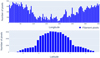 |
Fig. 2 Filament distribution along the longitude (top) and latitude (bottom) axis of the Galactic plane, from the catalogue of candidate filaments published in Schisano et al. (2020). The Galactic centre is located at (0°, 0°) (for the longitude, 0° corresponds to 360°). The bandwidth used to compute histograms is 1000 pixels for longitude and 50 for latitude. |
5.2.2 Position Encoding UNets
Position Encoding UNets make use of the position as an additional input. One may integrate an additional input such as the position encoding p (considering first that p ∈ ![Mathematical equation: $\[\mathbb{R}\]$](/articles/aa/full_html/2024/12/aa50828-24/aa50828-24-eq2.png) ) to a convolutional layer anywhere in the UNet by concatenating a new channel to the regular input channels of this convolutional layer, where the new channel is filled with the position encoding p (see Fig. 3 for illustration). Alternatively, if the position is encoded into two features (p ∈
) to a convolutional layer anywhere in the UNet by concatenating a new channel to the regular input channels of this convolutional layer, where the new channel is filled with the position encoding p (see Fig. 3 for illustration). Alternatively, if the position is encoded into two features (p ∈ ![Mathematical equation: $\[\mathbb{R}\]$](/articles/aa/full_html/2024/12/aa50828-24/aa50828-24-eq3.png) 2) as in our experiments, where the position is encoded as a (longitude, latitude) pair, one needs to concatenate two new channels, each one being filled with each of the two features.
2) as in our experiments, where the position is encoded as a (longitude, latitude) pair, one needs to concatenate two new channels, each one being filled with each of the two features.
While the position may be added at the input of the neural network, other choices may be made that correspond to different assumptions on how the position information may and should modify the filament detection decision. We investigated three alternatives which differ by the stage where the position information is added, either as an additional input, at the input of the model or in the middle hidden layer, or as a thresholding input (see Figure 4).
The most straightforward approach to add the position as input to the UNet consists of inputting the position as additional channels or maps at the input to the model, to the first convolutional layer (alternative 1, referred to as PE-UNet-I for PE-UNet-Input). This approach facilitates handling complex interdependencies between the patch itself and its position. Yet, one possible weakness of the approach is related to our previous observation (see Section 5.2.1) that a learnt UNet does not exploit the patch position: it is not clear whether the position information is strong enough for the optimization to rely on it. To overcome this difficulty we explore a second solution by inputting the position as additional channels to the first convolution layer of the decoder part of the UNet (alternative 2, namely PE-UNet-L for PE-UNet-Latent). Doing so could ease the use of this information by the model. In both cases it is possible for the UNet to take into account complex relationships between the patch and its position, for instance, the dependency between the orientation of a filament and the position of the patch it comes from. A last approach (alternative 3, in the following referred to as PE-UNet-D for PE-UNet-Decision) consists of inputting the position encoding before the last (decision) layer. We call this strategy a thresholding approach since this implementation makes that the output of the model FW(x) may be decomposed in two terms as ![Mathematical equation: $\[F_{W}(x)=F_{W}^{U n e t}(x)+H_{W}(p)\]$](/articles/aa/full_html/2024/12/aa50828-24/aa50828-24-eq4.png) where the first term is computed by the UNet component of the model and depends on the input patch x but not on its position and the second term HW(p) depends on the position of the patch only, p. Formulating computation this way, one sees that the decision of labelling a pixel as filament resumes to
where the first term is computed by the UNet component of the model and depends on the input patch x but not on its position and the second term HW(p) depends on the position of the patch only, p. Formulating computation this way, one sees that the decision of labelling a pixel as filament resumes to ![Mathematical equation: $\[F_{W}(x) \geq 0.5 \Leftrightarrow F_{W}^{U n e t}(x) \geq 0.5-H_{W}(p)\]$](/articles/aa/full_html/2024/12/aa50828-24/aa50828-24-eq5.png) . In other words, such a PE-UNet resumes to a UNet whose decision threshold is a function of the position, independently of the input patch. Of course, for such an implementation, the model cannot handle any relationship between the patch and its position.
. In other words, such a PE-UNet resumes to a UNet whose decision threshold is a function of the position, independently of the input patch. Of course, for such an implementation, the model cannot handle any relationship between the patch and its position.
The relative behaviour of the three strategies described above may help in getting insights into the validity of common hypotheses in the field (e.g. the orientation of filaments depends on their position). We note that we encoded both the longitude and the latitude coordinates of the position. To align with the results obtained by Schisano et al. (2020) and to facilitate neural network training alignment between, we propose to encode the position as a symmetrical function, with the centre of the Gp serving as the symmetrical centre. Furthermore, we ensure that the position encoding of a patch located at 360° corresponds to that of a patch located at 0° for longitude, to maintain circularity in our data. The position is encoded by the following function: ![Mathematical equation: $\[p_{l}=\frac{\left|l-l_{ {ref }}\right|}{l_{{range }}}\]$](/articles/aa/full_html/2024/12/aa50828-24/aa50828-24-eq6.png) where lref stands for the centre of the Galaxy is (180° for longitude and 0° for latitude) and lrange stands for the Gp coverage (360° for longitude and approximately 6° for latitude). l stands for both latitude and longitude. We note that, due to the Galaxy’s shape, real data might differ from the symmetry we adopt here. For example, two peaks are observed in the distribution of filaments in the Gp, one related to the Carina complex (l ≃ 280°) and one to the Cygnus system (l ≃ 80°) and on the third Galactic quadrant there is a lack of filamentary structures in the inter-arm region located between l ≃ 270–278° (Schisano et al. 2020, see their Fig. 2). Therefore some caveats may be associated with the symmetrical assumption we adopt here. However, even if the symmetrical property we adopt for the distribution of filament in the Gp might suffer some local departures, as mentioned above, we point out that, for machine learning, continuity and alignment between annotations and the features input are needed. Suggesting our neural network to learn a non-symmetrical spatial distribution while the labelling is showing every sign of a symmetrical one might be counter-productive during the optimization steps of neural network learning. On the other hand, one could try to learn directly filament segmentation given the filament spatial distribution under the form of constraint (neural network could learn filament segmentation while the filament spatial distribution respects a given one). But in order to do so, the distribution has to be known and explicitly expressed in the optimization process which is currently not the case for the filament distribution.
where lref stands for the centre of the Galaxy is (180° for longitude and 0° for latitude) and lrange stands for the Gp coverage (360° for longitude and approximately 6° for latitude). l stands for both latitude and longitude. We note that, due to the Galaxy’s shape, real data might differ from the symmetry we adopt here. For example, two peaks are observed in the distribution of filaments in the Gp, one related to the Carina complex (l ≃ 280°) and one to the Cygnus system (l ≃ 80°) and on the third Galactic quadrant there is a lack of filamentary structures in the inter-arm region located between l ≃ 270–278° (Schisano et al. 2020, see their Fig. 2). Therefore some caveats may be associated with the symmetrical assumption we adopt here. However, even if the symmetrical property we adopt for the distribution of filament in the Gp might suffer some local departures, as mentioned above, we point out that, for machine learning, continuity and alignment between annotations and the features input are needed. Suggesting our neural network to learn a non-symmetrical spatial distribution while the labelling is showing every sign of a symmetrical one might be counter-productive during the optimization steps of neural network learning. On the other hand, one could try to learn directly filament segmentation given the filament spatial distribution under the form of constraint (neural network could learn filament segmentation while the filament spatial distribution respects a given one). But in order to do so, the distribution has to be known and explicitly expressed in the optimization process which is currently not the case for the filament distribution.
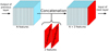 |
Fig. 3 Concatenation operation. We add position information as two additional channels or maps to the existing one already through a concatenation operation. The existing channels or maps can be either the density input or the results from a convolution layer (h and w being the channel or map size). We fill a h × w matrix with the position encoding pl. |
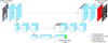 |
Fig. 4 Position Encoding UNet architecture. The model consists of a UNet architecture with the patch position as an additional input. Three alternatives of PE-UNet have been explored, Input (in orange), where we input the position as two additional channels before the first layer; Latent (in green), where we input the position as two additional features after the bottleneck; Decision (in red), where we input the position as two additional features before the last convolution. In our experiment, the PE-UNets are composed of five UNet blocks reducing the dimension to 2 × 2 × 1024 at the bottleneck level given a patch of size 32 × 32 × 1. |
6 Experimental study
6.1 Models optimization
The PE-UNet and all other neural architectures investigated here have been developed using Python 3.11.6 and Pytorch 2.0.1. We trained all models on Nvidia a40 GPU with 48GB VRAM with a batch size of 256 during a maximum of 100 epochs. An early stopping strategy was used: training was stopped if there was no loss improvement greater than 1 × 10⁻⁴ compared to the best loss during the last 10 epochs on the validation dataset. The ADAM scheme (Kingma & Ba 2014) was used to optimize the Binary Cross Entropy (BCE) loss with different initial learning rates (between 5 × 10⁻³ and 5 × 10⁻⁵, the initial learning rate being our only hyper-parameter) with the learning rate being divided by 10 every 10 epochs (Vojtekova et al. 2021). Both flips and rotations were used for data augmentation.
6.2 Metrics
In this section, we report a few metrics to quantitatively assess the performance of the models. Segmentation models output continuous values ranging from 0 to 1, representing the confidence of each pixel belonging to class 1 (filament class in our case). These values are binarized according to a threshold to yield a classification decision. When the models are learned to output target values {0, 1} for the two classes, as it is the case in our experiments (target filament class = 1 and target background class = 0), it is a common practice in machine learning to set the threshold at 0.5 (when learning data are balanced) at test time and classify as filament every pixel whose output is above 0.5 and as background all remaining pixels. One uses measures that integrate all possible threshold values to get a deeper idea of the behaviour of the classifier. This is particularly useful when the classes do not play a symmetric role (e.g. medical diagnosis, information retrieval) or when the true objective is that the score of samples from class 1 should be higher than the scores of samples from class 0, whatever the threshold.
We detail below the computation of the metrics we report in our experiments. We used two metrics that are thresholddependent, the Dice Similarity Coefficient (Wang et al. 2004) which is a widely used measure for semantic segmentation and the MSSIM, which has been introduced as a “Goodness-of-fit Measure” for filament detection by Green et al. (2017). We used a threshold of 0.5 to compute these metrics as it is consistent with the balance of our learning dataset (about 45% of pixels labelled as filaments and 55% as background). Additionally, we report mean Average Precision and Area Under the Curve Receiver Operating Characteristic at the pixel level, which are common in classification tasks, where both measures are averages over the threshold value.
DSC. The DSC corresponds to the f1 score at the pixel level. It gives more reliable information than the usual accuracy, especially in the presence of unbalanced data. It is defined as:
![Mathematical equation: $\[\mathrm{DSC}=\frac{2 \mathrm{TP}}{2 \mathrm{TP}+\mathrm{FP}+\mathrm{FN}}\]$](/articles/aa/full_html/2024/12/aa50828-24/aa50828-24-eq7.png) (1)
(1)
where TP stands for true positive (pixel labelled as filament and classified as such), FP stands for false positive (pixel labelled as background but classified as filament) and FN stands for false negative (pixel labelled as filament but classified as background). The DSC metric ranges from 0 to 1, and equals 1 when every pixel is correctly classified.
AUC ROC. The ROC curve is built from the classification performance of a model for any classification thresholds. It is given by plotting the true positive rate (also called Recall) against the false positive rate for each detection threshold:
![Mathematical equation: $\[T P R=\frac{T P}{T P+F N}\]$](/articles/aa/full_html/2024/12/aa50828-24/aa50828-24-eq8.png) (2)
(2)
![Mathematical equation: $\[F P R=\frac{F P}{F P+T N}.\]$](/articles/aa/full_html/2024/12/aa50828-24/aa50828-24-eq9.png) (3)
(3)
The AUC ROC summarizes the ROC curve into a single value by computing the area under the ROC curve. The AUC ROC value corresponds to the probability that the model ranks (in terms of output value) a random positive example (filament) higher than a random negative example (background). The score ranges from 0 to 1 with 1 meaning having a perfect separation (in terms of network output) between filament and background pixels.
mAP. The Average Precision summarizes the Precision-Recall curve (which shows the trade-off between correctly classified positive instances and true positive predictions among all actual positive instances) into one single value obtained by averaging precision over all the thresholds. The AP is given by the following equation:
![Mathematical equation: $\[\mathrm{AP}=\sum_{\mathrm{n}}\left(\mathrm{R}_{\mathrm{n}}-\mathrm{R}_{\mathrm{n}-1}\right) \mathrm{P}_{\mathrm{n}}.\]$](/articles/aa/full_html/2024/12/aa50828-24/aa50828-24-eq10.png) (4)
(4)
Here Rn and Pn are respectively recall (also called TPR) and Precision at the n-th threshold. The Precision is defined as follows:
![Mathematical equation: $\[\text{Precision} =\frac{\mathrm{TP}}{\mathrm{TP}+\mathrm{FP}}.\]$](/articles/aa/full_html/2024/12/aa50828-24/aa50828-24-eq11.png) (5)
(5)
The mAP is obtained by computing the mean AP over the test dataset.
MSSIM. The MSSIM (Wang et al. 2004) was originally designed to measure similarity between two images a and b in terms of luminance, contrast and structures at the pixel level. It is defined as
![Mathematical equation: $\[\operatorname{SSIM}(\mathrm{a}, \mathrm{b})=[\mathrm{l}(\mathrm{a}, \mathrm{b})]^{\alpha} \times[\mathrm{c}(\mathrm{a}, \mathrm{b})]^{\beta} \times[\mathrm{s}(\mathrm{a}, \mathrm{b})]^{\gamma}\]$](/articles/aa/full_html/2024/12/aa50828-24/aa50828-24-eq12.png) (6)
(6)
with α, β and γ being constants, and
![Mathematical equation: $\[l(a, b)=\frac{2 \mu_{a} \mu_{b}+C_{1}}{\mu_{a}^{2}+\mu_{b}^{2}+C_{1}}\]$](/articles/aa/full_html/2024/12/aa50828-24/aa50828-24-eq13.png) (7)
(7)
![Mathematical equation: $\[c(a, b)=\frac{2 \sigma_{a} \sigma_{b}+C_{2}}{\sigma_{a}^{2}+\sigma_{b}^{2}+C_{2}}\]$](/articles/aa/full_html/2024/12/aa50828-24/aa50828-24-eq14.png) (8)
(8)
![Mathematical equation: $\[s(a, b)=\frac{2 \sigma_{a b}+C_{3}}{\mu_{a} \mu_{b}+C_{3}}\]$](/articles/aa/full_html/2024/12/aa50828-24/aa50828-24-eq15.png) (9)
(9)
where μa, μb are the local means; σa, σb are the standard deviations; and σab is the cross-variance between images a and b. C1, C2 and C3 are small constants that are introduced to avoid instability of the MSSIM computation (Wang et al. 2004). Green et al. (2017) proposed to consider filament segmentation as a low-quality version of the density image and use the MSSIM to compare segmentation as output by different models. Hence while the MSSIM score is not fully relevant by itself, comparing two segmentations through the MSSIM scores computed with the same density/reference image may show genuine differences at the structural level (i.e. filaments). We note that the MSSIM is not a supervised metric (i.e. it is not based on the annotation used during training).
6.3 Comparison with our previous work
The UNet and UNet++ architectures used in this study are identical to those in Zavagno et al. (2023), yet the results differ significantly. In Zavagno et al. (2023), two regions of the Gp were excluded from the learning step for testing, and the models were trained in a single attempt without hyper-parameter selection on the remaining data. Moreover, due to the nonimplementation of randomization for the selection of patches, it was not possible to obtain a reliable segmentation of the whole Gp. Despite this, a comparison of several learning rates was performed. The work of Zavagno et al. (2023) was a proof-of-concept study to explore the potential of neural networks for filament’s identification over the Gp, in a supervised manner, using the masks of the existing filament catalogue (Hi-GAL) published by Schisano et al. (2020). Additionally, the UNet segmentation was able to remove catalogue artifacts caused by data noise and discover previously undetected filaments.
In contrast, this paper introduces a data distribution strategy that enables the segmentation of the entire Gp. During training, neural network hyper-parameters are optimized using a validation set, and performance across different architectures is compared for the whole Gp. Furthermore, this study compares the UNet and UNet++ architectures with two other models: the Swin-UNet and a new model we introduce that adds at different locations in the UNet architecture (see Fig. 1) the position of the patches in the Gp, the PE-UNet.
7 Results
In this section, we report and compare the results obtained using UNet and PE-UNet architectures. We first compare the models using the metrics presented in Section 6.2. This is an objective evaluation that provides useful insights but where the comparison concerns labeled pixels only (see Section 4.2), meaning that the behaviour of the models on ambiguous pixels (that may be the most interesting) is not taken into account. To go further and get a deeper understanding of how the models compare to each other we then visually analyze and compare the segmented maps obtained using the different models in Section 7.2.
7.1 Metric-based experimental study
In this section, we investigate the relative performance, with respect to the metrics defined above, of the three UNet baseline models, UNet, UNet++, SwinUNet and of the three PE-UNets (with three different ways of inputting the position information). In particular, we compare the relative performance of the three variants of PE-UNets.
We report comparative results obtained for the prediction of the full Gp using the strategy described in Section 5.1.1. Table 1 reports metrics where Column 1 presents the different architectures tested, Column 2 is the average DSC value across the 5 folds, Column 3 the average mAP value, Column 4 the average AUC ROC value and Column 5 the average MSSIM value, for each corresponding model. Table 2 reports significance results when comparing pairs of models using statistical tests, in particular, p-values obtained from paired t-tests (Yuen & Dixon 1973) performed on the DSC series for each pair of models (see Section 5.1.2). The null hypothesis is that the two sets of values come from two distributions with the same mean, and the confidence in rejecting the null hypothesis is given by the p-value, where a p-value below 0.05 indicates that the difference in performance between the two architectures under consideration is significant at a 95% confidence level.
First, we see that the PE-UNet-L model outperforms all other models whatever the metric, except for MSSIM where the PE-UNet-I gets the highest score. We note that the three metrics DSC, mAP and AUC ROC more or less provide the same ranking of the six models. We chose the DSC metric to perform a significance analysis of the results. Second, the PE-UNet-L significantly outperforms the three baseline models, with every p-value being below 0.05 (in bold in Table 2). Finally, the three metrics DSC, mAP and AUC ROC are quite consistent but the MSSIM metric strongly disagrees with these. After a deeper analysis presented in Appendix D, we conclude that the MSSIM metric is not reliable enough and we do not draw any conclusion from the results obtained with this metric. We report MSSIM results as MSSIM is a standard metric used in the filament detection field but unfortunately after investigating the impact of the hyperparameters on the MSSIM metric we found that conclusions one may draw may vary depending on the chosen hyperparameters (refer to Appendix D for additional details), making this metric less reliable than expected.
Next, we investigate the impact of the position encoding location within the model. As shown in Table 1, encoding the position in the latent space yields better results across the three classification metrics (DSC, mAP, AUC ROC). According to the significance tests (Table 2), the PE-UNet-L significantly outperforms PE-UNet-D where the position is input to the decision layer. On the other hand, there does not seem to be significant differences between encoding the position at the input or at the intermediate layer (p-value of 0.1676).
We also note that the performance of the PE-UNet-I and of the PE-UNet-D are not significantly different while the PE-UNet-L is the only PE-UNet architecture that is significantly better than the other models (UNet, UNet++ and SwinUNet).
Comparative results of segmentation models.
Significance results for comparing models.
7.2 Comparison of models’ performance with segmentation maps
Results using metrics (see Section 7.1) give the architecture that best recovers, at the pixel level, the input annotation for filament and background masks (see Section 4.2 for details). As presented in Table 1 the DSC metric obtained for PE-UNet-L gives a 97.46% accuracy on the recovery of the labelled data. However, due to the known incomplete labelling over the Gp (refer to Section 4.2), we have no guarantee that this value is valid for the remaining part of the Gp. In order to obtain this result, we construct segmentation maps of the Gp to check if the indication given by the metrics on the best model corresponds to the targeted astrophysical results obtained for the segmented maps, i.e. the robust detection of filaments over a large range of density, including low-contrast and low-density ones. In particular, we are interested in checking how realistic are the structures detected, because we have no absolute ground truth for the filament class. Segmentation maps are obtained after computing the segmentation of every patch of the Gp and then binarizing the continuous maps using a threshold of 0.5 (see Section 6.2 for threshold discussion). The detailed procedure can be found in Appendix E. From those segmentation maps, we use the normalized map as a reliable proxy for filamentary structures. This hypothesis is discussed on an empirical basis in Section 7.2.1. In the following, we compare segmentation maps obtained with the different architectures presented in Section 7.1. We note that in all the following figures, the representations are given in Galactic coordinates and north is up and east is left.
7.2.1 Local min-max normalized column density map
In order to gain a deeper insight into the data used by our models during both the training phase and the segmentation of the Gp, we reconstruct a map of the entire Gp after normalization being applied. The local min-max normalization performs a background subtraction on a local spatial scale (at the scale of a patch, i.e. 32 × 32 pixels), revealing low-contrast filaments that are not seen on the original column density map. The way we use this map is presented in this Section, in particular its astrophysical interest and its use for validation of our results. We note that the high dynamical range observed on Hi-GAL column density images makes challenging the optimal visualization of these images. For this purpose, Li Causi et al. (2016) have developed a multi-scale algorithm to optimize the visualization of the Herschel Hi-GAL images of the Gp allowing for optimized visualization of both high- and low-contrast emission.
The resulting normalized column density map we create is shown for two characteristic column density zones of the Gp, a low-density region centred at (l, b)=180.19°, 0° (see Figure 5, with a mean-max column density range of 1 × 10²¹ to 2 × 1022 cm−2) and a high-density region centred at (l, b) = 332°, 0° (see Figure 6, with a mean-max column density range of 6 × 10²¹ to 1 × 1023 cm−2). This normalized map of the whole Gp has numerous advantages: by removing the local background it reveals clearly the filamentary structure of the medium in both low- and high-density regions of the plane. As no absolute ground truth exists for filaments, in the following we use this map, together with data obtained at other wavelengths (with telescopes other than Herschel), to validate the detection of filaments by the different models. This validation is based on visual inspection. Before their final individual confirmation which is ongoing but beyond the scope of this paper, all the filaments described in the following are candidate filaments. We note that the normalization process erases important physical information associated with a given structure such as column density and mass. However, the information can be easily recovered by reprojecting the structure on the original column density map.
The filamentary structures observed on this normalized map exhibit different configurations that will drive the future learning of what a filament is by the different architectures used. In the following we consider as candidate filament an elongated structure with an aspect ratio >3 (see Kumar et al. 2020) observed on the normalized column density map. Most of the filaments host compact sources that are not removed from the map before the learning process. This means that the ensemble (filament+sources) is learnt and further segmented. In the following we use the generic term filament to describe this ensemble, keeping in mind that they are only candidates at this stage.
Two categories of filaments are observed on the normalised column density map: high-contrast filaments that have a peak emission/local background >2 on the original column density map and that are already well structured as elongated (aspect ratio >3) emission in the original map and low-contrast filaments (that have a peak emission/local background <2 on the original column density map. These two categories of filaments are observed in both low and high column density zones of the Gp. We define the local background on the original column density map as the average emission level that is observed in the immediate surrounding region (<6 pixels) around the filament. Examples of these high- and low-contrast filaments are shown with cyan and yellow arrows, respectively on Figure 5 (a low-density region of the Gp) and Figure 6 (a high-density region of the Gp). High-contrast filaments are characterized by bright structures that sit on a very low local emission on the normalized emission map (dark zones on the normalized map). These high-contrast structures are well seen on the normalized input map and are easily recognized (associated pixels classified as filament) by the different networks. The low-contrast filaments, which are barely seen on the original column density map, are revealed clearly by the local min-max normalization process and so appear well on the normalized column density map (see Figure 5). Compared to the high-contrast filaments, their appearance is fluffier and they are, in some cases, less well-detached from their surrounding emission on the normalized map but they are detected by the networks as long as they appear as elongated structures (aspect ratio > 3). Their detection score is particularly high with the PE-UNet-L segmentation. The last type of emission that appears on the normalized column density map is a local, diffuse and non-structured emission that is not classified as filament by the networks. As observed in Figures 5 and 6, the normalized column density map reveals a highly filamentary medium, where high-contrast filaments appear thin, very well defined and well detached from their surrounding whereas lower contrast filaments appear larger and fluffier. We note that the presence of compact sources associated with these filaments is also particularly well-revealed by the normalization process.
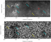 |
Fig. 5 Comparison of the column density map (top) and the corresponding local normalized column density image (bottom) on a low-density region of the Gp centred at (l, b) = 181°, 0°. Examples of high- and low-contrast filaments (discussed in the text) present on the original column density map (top) and their counterparts on the normalized map (bottom) are identified with cyan and yellow arrows, respectively. The red square (top) shows a 32 × 32 pixels box over which the normalization is performed. The original column density map is represented in logarithmic scale and spans the range 1 × 10²¹ to 2 × 1022 cm−2. |
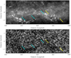 |
Fig. 6 Comparison of the column density map (top) and the corresponding local normalized column density image (bottom) on a high-density region of the Gp centred at (l, b) = 332°, 0°. Examples of high- and low-contrast filaments (see text) present on the original column density map (top) and their counterparts on the normalized map (bottom) are identified with cyan and yellow arrows, respectively. The original column density map is represented in logarithmic scale and spans the range 6 × 10²¹ to 1 × 1023 cm−2. The white and black squares on the original column density and normalized map, respectively, are saturated regions. |
7.2.2 Comparison of the Hi-GAL normalized column density map with 12CO(3—2), 2MASS and Spitzer data
A way to ascertain the nature of the structures (filaments and compact sources) observed on the normalized map is to use data obtained at other wavelengths that trace well the density of the interstellar medium. In the following, we use both near- and mid-infrared data and millimeter spectroscopic data to ascertain the nature of some of the observed structures. In particular, we use the 12CO (3–2) High-Resolution Survey (COHRS) of the Galactic Plane (Park et al. 2023) that covers the ![Mathematical equation: $\[9^{\circ}_\cdot5 \leq l \leq 62^{\circ}_\cdot3\]$](/articles/aa/full_html/2024/12/aa50828-24/aa50828-24-eq16.png) and
and ![Mathematical equation: $\[|b| \leq 0^{\circ}_\cdot5\]$](/articles/aa/full_html/2024/12/aa50828-24/aa50828-24-eq17.png) range with a spatial resolution of
range with a spatial resolution of ![Mathematical equation: $\[16^{\circ}_\cdot6\]$](/articles/aa/full_html/2024/12/aa50828-24/aa50828-24-eq18.png) and a spectral resolution of 0.635 km/s. Because we work on 2D data, we use the 2D version of the COHRS spectroscopic data that corresponds to the 3D cube integrated over the observed velocity range (Park et al. 2023). At this stage, because we work with 2D data, we do not add information about the velocity structure of the filament masks we use. We note that, using 13CO (2–1) and C18O (2–1) data of the SEDIGISM survey (Structure, Excitation, and Dynamics of the Inner Galactic Inter Stellar Medium), Mattern et al. (2018) show that 70% of the filaments they studied are velocity coherent. Figure 7 shows a comparison of the 12CO (3–2) velocity-integrated COHRS map and the normalized column density map centred at (l, b) = 16.5°, 0°. Although not at the same spatial resolution and sampling different excitation conditions of the ISM, the two maps present clear similarities, including the presence of filamentary structures and bright compact sources, as underlined in Fig. 7. We note also that no background has been subtracted on the COHRS 2D image, rendering the one-to-one comparison between the two maps difficult. Based on a visual inspection, the same comparison has been lead on the whole COHRS 12CO (3–2) velocity-integrated image and confirms on both low and high column density regions that compact sources and filamentary structures identified on the normalized column density map have counterpart in the molecular range, confirming their real existence and validating our use of the normalized map to ascertain the ensemble (compact sources + filamentary structures) observed on the segmented map. Data at other wavelengths can also be used to validate the use of the normalized column density map to validate the classification given by the segmented map. As shown in Figure 8 2MASS data (Skrutskie et al. 2006) confirm that the filamentary structures observed on the normalized column density map correspond to dark absorption zones in the near-infrared, as expected for dense absorbing regions of the Galactic ISM made of gas and dust. The mid-infrared domain can also be used to ascertain the nature of structures observed on the normalized column density map. Dense regions of the ISM appear as dark features in this spectral range. In particular, the infrared dark clouds (IRDCs) identified with Spitzer data (Peretto & Fuller 2009) have opened an important field of research for star formation, as representing the location for the formation of stellar protocluster. Recent works show how active is this field of research (Rigby et al. 2024; Reyes-Reyes et al. 2024; Izumi et al. 2024). Figure 9 presents a comparison of the velocity-integrated COHRS map with the normalized columndensity map, the original Hi-GAL column density map and the Spitzer-IRAC 3.6 μm (orange) and 4.5 μm (red) GLIMPSE 360 mid-infrared data (Whitney et al. 2011) of a portion of the Gp centred at the location (l, b) = 10.50°, −0.18°. This region has been chosen as an illustrative example at it hosts the well-known Galactic infrared dark cloud, the ‘Snake’, G11.11–0.12 (Pillai et al. 2006). This structure is underlined with a red arrow in Figure 9. Well-seen in absorption on the two colour-composite 3.6 μm (orange) and 4.5 μm (red) Spitzer-IRAC GLIMPSE 360 image, this dark cloud is clearly seen in emission on both the Hi-GAL column density map and on the normalized map. We note that the compact sources present in this IRDC are well-revealed on the normalized map. We note that this cold and dense feature is barely detected on the velocity-integrated COHRS map (see Figure 9) due to its low temperature (Wang et al. 2014; Dewangan et al. 2024).
and a spectral resolution of 0.635 km/s. Because we work on 2D data, we use the 2D version of the COHRS spectroscopic data that corresponds to the 3D cube integrated over the observed velocity range (Park et al. 2023). At this stage, because we work with 2D data, we do not add information about the velocity structure of the filament masks we use. We note that, using 13CO (2–1) and C18O (2–1) data of the SEDIGISM survey (Structure, Excitation, and Dynamics of the Inner Galactic Inter Stellar Medium), Mattern et al. (2018) show that 70% of the filaments they studied are velocity coherent. Figure 7 shows a comparison of the 12CO (3–2) velocity-integrated COHRS map and the normalized column density map centred at (l, b) = 16.5°, 0°. Although not at the same spatial resolution and sampling different excitation conditions of the ISM, the two maps present clear similarities, including the presence of filamentary structures and bright compact sources, as underlined in Fig. 7. We note also that no background has been subtracted on the COHRS 2D image, rendering the one-to-one comparison between the two maps difficult. Based on a visual inspection, the same comparison has been lead on the whole COHRS 12CO (3–2) velocity-integrated image and confirms on both low and high column density regions that compact sources and filamentary structures identified on the normalized column density map have counterpart in the molecular range, confirming their real existence and validating our use of the normalized map to ascertain the ensemble (compact sources + filamentary structures) observed on the segmented map. Data at other wavelengths can also be used to validate the use of the normalized column density map to validate the classification given by the segmented map. As shown in Figure 8 2MASS data (Skrutskie et al. 2006) confirm that the filamentary structures observed on the normalized column density map correspond to dark absorption zones in the near-infrared, as expected for dense absorbing regions of the Galactic ISM made of gas and dust. The mid-infrared domain can also be used to ascertain the nature of structures observed on the normalized column density map. Dense regions of the ISM appear as dark features in this spectral range. In particular, the infrared dark clouds (IRDCs) identified with Spitzer data (Peretto & Fuller 2009) have opened an important field of research for star formation, as representing the location for the formation of stellar protocluster. Recent works show how active is this field of research (Rigby et al. 2024; Reyes-Reyes et al. 2024; Izumi et al. 2024). Figure 9 presents a comparison of the velocity-integrated COHRS map with the normalized columndensity map, the original Hi-GAL column density map and the Spitzer-IRAC 3.6 μm (orange) and 4.5 μm (red) GLIMPSE 360 mid-infrared data (Whitney et al. 2011) of a portion of the Gp centred at the location (l, b) = 10.50°, −0.18°. This region has been chosen as an illustrative example at it hosts the well-known Galactic infrared dark cloud, the ‘Snake’, G11.11–0.12 (Pillai et al. 2006). This structure is underlined with a red arrow in Figure 9. Well-seen in absorption on the two colour-composite 3.6 μm (orange) and 4.5 μm (red) Spitzer-IRAC GLIMPSE 360 image, this dark cloud is clearly seen in emission on both the Hi-GAL column density map and on the normalized map. We note that the compact sources present in this IRDC are well-revealed on the normalized map. We note that this cold and dense feature is barely detected on the velocity-integrated COHRS map (see Figure 9) due to its low temperature (Wang et al. 2014; Dewangan et al. 2024).
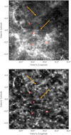 |
Fig. 7 Comparison of the COHRS 12CO (3—2) velocity-integrated image (top) and the corresponding local normalized column density image (bottom) on a low-density region of the Gp centred at (l, b) = 16.5°, 0°. The compact sources (red circles) and filamentary structures (orange arrows) seen on the two maps are underlined. The COHRS image is represented in a linear scale with an intensity that spans the range of 0–80 K km/s. |
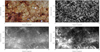 |
Fig. 8 Comparison of the 2MASS JHKS colour image (top left), normalized column density map (top right), column density map (bottom left) and COHRS 12CO (3–2) velocity-integrated image (bottom right) in a low-density region of the Gp centred at (l, b) = 16°, 0°. The original column density is displayed in logarithmic scale and spans the range 3 × 10²¹ to 5 × 1022 cm−2. The COHRS image is represented in a linear scale with an intensity that spans the range of 0–70 K km/s. |
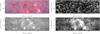 |
Fig. 9 Comparison of GLIMPSE 3603.6 μm (orange) and 4.5 μm (red) Spitzer-IRAC image (top left), the normalized column density map (top right), the column density map (bottom left) and the COHRS 12CO (3–2) velocity-integrated image (bottom right) in a region of the Gp centred at (l, b) =10.50°, −0.18°. Weote the presence of the infrared dark cloud G11.11–0.12, the Galactic ‘Snake’, identified by the red arrow. The original column density is displayed logarithmic scale and spans the range 1 × 10²¹ to 1 × 1023 cm−2. The COHRS image is represented in a linear scale with intensity that spans the range of 0–100 K km/s. |
7.2.3 Comparison of UNet-based segmentation maps
We compare the results obtained by the different models using the segmentation maps, in particular the differences observed between the different versions of UNet with no encoding of the position, namely, UNet, SwinUNet, UNet++ and the three versions of the model with position encoding (PE-UNet-I, PE-UNet-L, and PE-UNet-D). As concluded using the metrics and as observed on the segmentation maps, the different models all performed very well in recovering the input filamentary structures. In particular, the high-contrast, high-density filaments are detected by all models with the particularity, for the SwinUNet to broader all the detected structures, compared to the other models. On the newly detected filaments, the UNet, SwinUNet and UNet++ are more able to detect structures associated with noise than PE-UNet, with SwinUNet performing even better than UNet++ in these zones. SwinUNet shows good performance on low-contrast structures when the local emission observed around the structures is low, as observed, for example, at high latitudes above the plane in high-density regions, on the edges of the map. This effect is not observed for UNet++. Towards high-density regions, the differences between PE-UNet-L are higher (compared to SwinUNet) than to UNet++, with a higher level of detection towards the central part of the plane.
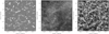 |
Fig. 10 Comparison of the segmented maps obtained using the PE-UNet-L and UNet versions centred on a low column density region of the plane at the location around l = 163°, 0°. The difference between the two segmented maps (PE-UNet-L – UNet) is shown (left) with the corresponding column density map (middle) and local normalized column density map (right). The white (black) features seen on the left map correspond to features detected with the PE-UNet-L (UNet) only. |
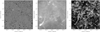 |
Fig. 11 Comparison of the segmented maps obtained using the PE-UNet-L and UNet versions centred on a high column density region of the plane at the location around (l, b) = 353°, 0°. The difference between the results of the two segmented maps (PE-UNet-L – UNet) is shown (left) with the corresponding column density map (middle) and the local normalized column density map (right). The white (black) features seen on the left map correspond to features detected with the PE-UNet-L (UNet) only. |
7.2.4 Comparison of PE-UNet-Latent and UNet segmentation maps
Because PE-UNet-L appears as the best model according to the metrics, in the following we focus the comparison on the segmented maps produced by PE-UNet-L and UNet. This comparison aims at understanding what brings the position encoding for the detection of filaments, using the UNet architecture. On the whole Gp, the difference between the two segmented maps (PE-UNet-L – UNet) is non-uniform over the plane and shows important variations as a function of the longitude and latitude positions, with a dominance of the PE-UNet-L detections towards lower density regions (132–208°), compared to the UNet in higher density regions (0–36°). This confirms that the position encoding in the latent space introduces a dependence on the detection of filaments. A close-up view on regions characterized by either low or high column density reveals a more complex behavior, as illustrated in Figures 10 and 11. The difference of the two segmented maps (PE-UNet-L – UNet) is presented on two characteristic column density regions of the plane, i.e. the central part (high-density region) centred at (l, b) = (353°, 0°) and a low-density region centred at (l, b) = (163°, 0°). As seen in Figures 10 and 11, the first clear difference between the PE-UNet-L and UNet segmentation resides in the clear longitude- and latitude-dependence on the detection of new filamentary structures. Compared to the segmented map obtained using UNet, the one obtained using PE-UNet-L shows an increase in the number of new pixels classified as filament in the low-density region (78% more pixels classified as filament for Figure 11) whereas the detection is not changed too much in the high-density region (11% fewer pixels classified as filaments for Figure 10). This suggests that the PE-UNet-L model is particularly sensitive to low-contrast structures at the same time as being able to detect high-contrast ones.
In regions of high-contrast and high-density, no clear differences are observed between PE-UNet-L and Unet, suggesting that PE-UNet-L particularly acts in low-density regions on low-contrast structures. However, some low-density regions, such as the one centred around l = 129° show little differences between the two segmented maps, suggesting that another factor (other than the characteristic density or the contrast) is responsible for the observed differences. Some regions of the plane are associated with a higher level of data noise in the data that is enhanced by the normalization process, observed in both low-density (around l = 129°) and high-density regions (around l = 345°). This results in a good detection of the noisy structures by the UNet but a lower detection by the PE-UNet-L, suggesting that this last is more sensitive to the noise. UNet detects structures associated with a higher level of noise, with a higher score than the PE-UNet-L. This statement is seen in both high- and low-density regions of the Gp and only depends on the local level of noise. The different sources of noise present in the original Hi-GAL data are discussed in detail in Zavagno et al. (2023, Appendix A). These regions are masked during the training process and so treated with caution on the segmented maps. When analyzing filaments in noisy regions, we favour the UNet model.
Compared to UNet, PE-UNet-L allows the detection of new structures, in particular the low-contrast ones that are barely seen on the original column density map but that are better revealed on the normalized map. PE-UNet-L particularly performs over UNet in regions where the contrast (structure/background) on the original column density map is low (a few percent) and where the local background is more uniform (and so easier to remove), leading to a strong enhancement of the low-density structures on the normalized map. These structures are particularly well detected by the PE-UNet-L. This is illustrated in Figure 12. The structures seen in white on Figure 12 (top left) correspond to low-contrast filaments that are barely seen on the original column density image (see Figure 12 (top right)). This sensitivity to lower contrast emission from the PE-UNet-L is also responsible for the contouring effect observed, as illustrated on Figure 12 (top left) where white contours are observed and correspond to the extension of higher contrast filaments that are detected by the UNet, but not their lower contrast surrounding part. This translates into a new contouring feature, observed around the structures previously detected by the UNet. This effect shows a clear dependence on the Galactic position and is mainly driven by the local background that creates lower-contrast emissions around higher-contrast filaments. Filaments detected previously by the UNet appear now slightly extended on the difference map. This extension corresponds to a lower-contrast density emission to which the PE-UNet is more sensitive. The new detections are particularly found in regions of low intensity for features that have low contrast (a few percent above the local background). Although barely seen on the column density map (see Figure 12), these structures are better revealed on the normalized map. The detection is even better when the background is low and more uniform on the original column density map.
As seen in Figure 13 a drastic change in the behavior of the difference map is observed at the position centred at (l, b) = 305°, 0°. This change is driven by the change in the original column density map (more diffuse and homogeneous emission at l < 305°, more structured and with higher emission contrast for l > 305°). This results in a minor difference between PE-UNet and UNet, confirming that, compared to the UNet, the optimal range of action of PE-UNet-L is for lower contrast structures.
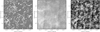 |
Fig. 12 Comparison of the segmented maps obtained using the PE-UNet-L and UNet versions centred on a high column density region of the plane at the location around (l, b) = 144°, 0.3°. The difference between the result of the two segmented maps (PE-UNet-L – UNet) is shown (left) with the corresponding column density map (middle) and the local normalized column density map (right). The white features seen on the left map correspond to features detected only with the PE-UNet-L. |
7.2.5 Comparison of UNet-based segmentation maps with previous filaments detection from Schisano et al
Results from metrics presented in Section 7.1 show that UNet-based models recover from 96 to 97% of the input annotation (for both filaments and background) at the pixel level. In this Section we present a comparison of the segmented maps of the whole Gp created using UNet-based models with the map of the input filament masks from Schisano et al. (2020). The idea is to ascertain the nature of the new detected structures and to discuss their properties.
In Figure 14 and Figure 15 we present the comparison of structures detected with the PE-UNet-L with the ones that were previously detected by Schisano et al. (2020), in two characteristic regions of the Gp at low and high column density, respectively. We chose the PE-UNet-L segmentation map for the comparison as it results from the best of all tested models.
Structures detected previously by Schisano et al. (2020) are detected by all the UNet-based architectures, with their width slightly enlarged. This was already observed with the UNet and corresponds to the fact that the masks used as inputs trace only the crest of the filament (Zavagno et al. 2023, see their Section 4.3 and figure 21) and that the structures observed on the normalized map are often associated with a more diffuse emission that is likely to belong to the structure itself as a local background has been removed.
The difference is more pronounced in the low-density regions of the Gp where a high number of new low-contrast and low-density structures are now detected with the UNetbased architectures. Compared to the input masks, all the newly detected structures observed on the segmentation map correspond to the structured emission observed on the normalized column density map. As presented in Section 7.2.1 most of these structures correspond to both absorption in the near- and mid-infrared and to emission in the millimeter ranges, indicating their nature as filamentary molecular clouds.
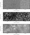 |
Fig. 13 Comparison of the segmented maps obtained using the PE-UNet-L and UNet at location around (l, b) = 305°, 0°. The difference between the binarized PE-UNet-L and UNet segmentation maps (top), the normalized column density map (middle), and the original column density map (bottom) are shown. The white (black) features seen on the top map correspond to features detected with the PE-UNet-L (UNet) only. |
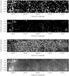 |
Fig. 14 Comparison of the segmented map obtained using (from top to bottom) the PE-UNet-L and the original input mask map detected by Schisano et al. (2020) at the location around (l, b) = 180°, 0°. The original and normalized column density maps are also shown. |
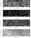 |
Fig. 15 Comparison of the segmented map (from top to bottom) obtained using the PE-UNet-L and the original input mask map detected by Schisano et al. (2020) at the location around (l, b) = 308°, 0°. The original and normalized column density maps are also shown. |
7.2.6 Comparison of PE-UNet segmentation maps
After showing that the PE-UNet-L model offers a significant improvement compared to UNet, in particular in the detection of low-contrast filaments, we discuss here the differences observed between the three PE-UNet versions tested. We recall that the difference between these three models resides in the location of the patch position encoding in the network (see Figure 4). The idea here is to explore the impact the position encoding’s place in the architecture has on the detection of the structures.
Results of the corresponding segmented map on two characteristic zones of the plane are shown in Figure 16 (for the low-density region) and Figure 17 (for the high-density region). On the two representative regions of the Gp, similar detections are observed for the three versions of the PE-UNet, all corresponding well to structured emission observed on the normalized column density map. Local variations are observed on a smaller spatial scale for low-contrast filaments that are better detected by both PE-UNet-D and PE-UNet-L compared to PE-UNet-I that tend to miss these, the best performance (highest score on the segmented map) being obtained by PE-UNet-L.
On the whole Gp, the behavior of the three versions for structure detection depends on the position (longitude and latitude) in the plane. High-contrast filaments (associated with a dark surrounding on the normalized map) are well-detected by all three versions, the higher score being obtained for PE-UNet-L. The main difference observed between the three versions of PE-UNet is in the robustness of the model to the noise present in the data. PE-UNet-I and PE-UNet-D are more robust for the detection of structures in regions where a higher noise level is observed (overlapping regions that connect successive tiles; see e.g. Zavagno et al. (2023, Fig. A1) for a discussion of the different noise sources present in the Hi-GAL data). They detect structures there that are not detected by PE-UNet-L, PE-UNet-I being more efficient than PE-UNet-D in these cases. As for the comparison with UNet, we recall that noisy regions are treated with caution on the segmented maps and are excluded from the training and learning process. In high-density regions of the Gp PE-UNet-I better detects structures than the PE-UNet-L on the edges (latitude |b|) >0.6°) of the plane where the level of emission on the original column density image becomes significantly lower (decreases by a factor of 2). In the mid-plane, where the emission on the original column density map is very high, PE-UNet-L detects more low-contrast structures than PE-UNet-I.
To summarize this Section, PE-UNet-L gives the best performance for structure detection compared to PE-UNet-I and PE-UNet-D in regions of the Gp not affected by noise. In this case, PE-UNet-I is more robust and able to detect structures associated with noise.
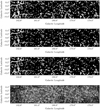 |
Fig. 16 Comparison of the segmented maps (from top to bottom) obtained using the three PE-UNet versions at the low-density location centred on (l, b) = 180°, 0°: PE-UNet-I, PE-UNet-D, PE-UNet-L. The corresponding normalized column density map is also shown. |
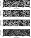 |
Fig. 17 Comparison of the segmented maps obtained using the three PE-UNet versions at the dense location centred on (l, b) = 308°, 0° (from top to bottom): PE-UNet-I, PE-UNet-D, PE-UNet-L. The corresponding normalized column density map is also shown (bottom). |
7.2.7 Generalization of the trained model: Segmentation of the 12CO (3–2) COHRS dataset
Generalizability for image segmentation is one of the major challenges in deep learning, in particular for medical imaging (Torpmann-Hagen et al. 2022). The huge amount of data available for the Gp makes the study of generalization of the model trained important. In this Section, we evaluate the generalization capability of our model by applying it to segment the 2D (position, position) velocity-integrated version of the 3 D (position, position, velocity) 12CO (3–2) COHRS dataset with a model trained on the NH2 Hi-GAL dataset. We proceed as follows: We use the COHRS 12CO (3–2) velocity integrated map publicly available at doi:10.11570/22.0078 that gives a 2D (position, position) emission map at the original resolution of ![Mathematical equation: $\[16^{\circ}_\cdot6\]$](/articles/aa/full_html/2024/12/aa50828-24/aa50828-24-eq19.png) . Then we smooth this map to the resolution of 36″ that corresponds to the spatial resolution of the Hi-GAL column density map, using the reproject_adaptive function in the python reproject package. From this newly created image we extract a series of 32 × 32 pixels patches with a stride of 1 (resulting in an overlap of 31 pixels), as we did for the column density image of the Gp (see Appendix E). All patches are then normalized using the local min-max normalization described in Section 4.3. The patches are then segmented using the PE-UNet-L model learnt on NH2 data. The final stage is the creation of the segmented map for the whole 2D COHRS map by combining and averaging all the patches (see Appendix E for details). The obtained segmented map is then binarized to a threshold of 0.5. The result of the velocity-integrated 2D 12CO (3–2) COHRS segmentation is presented in Figure 18 where the model learnt on NH2 data using the PE-UNet-L architecture has been applied to the COHRS 2D map. The inference time to obtain the COHRS segmentation maps is about 12 hours.
. Then we smooth this map to the resolution of 36″ that corresponds to the spatial resolution of the Hi-GAL column density map, using the reproject_adaptive function in the python reproject package. From this newly created image we extract a series of 32 × 32 pixels patches with a stride of 1 (resulting in an overlap of 31 pixels), as we did for the column density image of the Gp (see Appendix E). All patches are then normalized using the local min-max normalization described in Section 4.3. The patches are then segmented using the PE-UNet-L model learnt on NH2 data. The final stage is the creation of the segmented map for the whole 2D COHRS map by combining and averaging all the patches (see Appendix E for details). The obtained segmented map is then binarized to a threshold of 0.5. The result of the velocity-integrated 2D 12CO (3–2) COHRS segmentation is presented in Figure 18 where the model learnt on NH2 data using the PE-UNet-L architecture has been applied to the COHRS 2D map. The inference time to obtain the COHRS segmentation maps is about 12 hours.
The segmentation of the 2D COHRS map obtained shown on Figure 18 (bottom left) well corresponds to the structured emission observed on the normalized COHRS map shown on Figure 18 (top left) suggesting that the filamentary molecular clouds are well recovered by the generalization process. Regions associated with a higher level of noise in the original 2D COHRS map observed at latitude b = 0.25°) are not well treated by the segmentation process and appear as round dense zones on the segmented map (see Fig. 18 bottom left), clearly different in shape from the detected filamentary structures seen on the map. This is due to the fact that the PE-UNet-L model is not well adapted to the detection of structures associated with a high level of noise (see Section 7.2.4 for a discussion).
Although tested only on the 2D version of the COHRS spectroscopic dataset, this result is promising to envision the generalization of this process to a larger dataset. Noise present in the data is a clear limitation to this generalization process. However, promising methods of denoising based on deep learning (Liu & Liu 2019; Li 2023) offer opportunities to ease the use of generalization on a large sample of datasets.
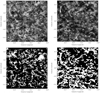 |
Fig. 18 Segmentation of the velocity-integrated 2D (position, position) 12 CO (3–2) COHRS map using the model learnt on the column density image of the Gp with PE-UNet-L at the location centred at (l, b) = 16.5°, 0°. The min–max normalized COHRS (top left) and NH2 (top right) maps are shown. The corresponding segmented maps using the PE-UNet-L learnt model on NH2 data are shown for COHRS (bottom left) and NH2 (bottom right). |
8 Discussion
We now discuss the results presented in Section 7.1 and 7.2. We have shown that the position encoding in the latent space with the PE-UNet-L architecture gives the best performance when comparing both metrics and pixels’ classification on the segmentation maps. In particular, the PE-UNet-L is able to detect low-contrast low-density filaments, that other UNet-based models barely detect while having similar results for high-contrast high-density filaments. Those low-contrast low-density filaments were previously not detected. In the following, we discuss the impact of the data augmentation, including the rotation of the patches, on the learning process.
8.1 Data augmentation
Data augmentation is a classical strategy used in the deep learning community to increase the size of the training set and get better performance. It consists of applying a set of transformations T ∈ 𝒯 to the data samples such that if (x, y) is a labeled training sample, then {(T(x), y), T ∈ 𝒯} are additional valid training samples (i.e. belong to the same distribution as one of the training samples, e.g. {(x, y)}). A popular particular case is transformations which are known to preserve the supervision information for the task at hand. For instance when considering object recognition tasks, one knows that rotations and flips do not change the supervision (i.e. the class label) of an image (e.g. a rotated chair is still a chair) so such augmentation strategies are extensively used for learning computer vision systems.
While these standard image data augmentation strategies might be used on our data, we argue that this should be done carefully. For instance, a filament’s orientation might depend on its position as it is related to the physical properties of its surrounding medium, e.g. the orientation of the magnetic field. Then any transformation that modifies the orientation of a patch (e.g. and of the included filament if any) may break such an underlying dependency, e.g. between the patch itself, its position and the orientation of a filament it includes, if any. This would make that rotated samples (T(x), y) do not obviously belong to the same distribution as regular training samples (x, y).
This is particularly true if the model takes into account the position of the patch it processes, as PE-UNet models do. In this latter case we note an input sample as a pair (x, p) of a patch, x, and of its position, p, and also note a labelled training sample as ((T(x), p), y). Then applying a transformation T to the patches should satisfy the property that applying the set obtained by transformation T the training data, {((T(x), p), y)}, follow the same distribution as original training samples {((x, p), y)}. But according to the discussion above this would not be true as, in an augmented sample ((T(x), p), y), a rotated patch T(x) could not match the original position p.
Yet, the conclusion of this discussion is not immediate. Although using an unsuitable data augmentation strategy may harm the learning of the model, at the same time, it allows an increase in the size of the training set, which is known to systematically improve the performance of a machine learning model. At the end, the two effects play in opposite directions and the issue depends on how unsuitable the data augmentation strategy is. We therefore designed experiments to analyse further the impact of the rotation and flips as an augmentation strategy in our experiments. The first question we address is: Do non-orientation-preserving augmentation strategies lead to a significant gain in performance? To answer this question we compared the performance of two models, the UNet and the PE-UNet-L, when learned either without, or with data augmentation (flips and rotations) (see Table 3).
For both models, the use of data augmentation significantly improves performance for all the metrics (we do not consider the MSSIM metric here for reasons explained previously). The second question is: How much does the unsuitability of the data augmentation strategy hurt? The answer lies in the comparison of the performance gain one observes when using data augmentation, between the UNet model and the PE-UNet-L model. As the UNet model does not exploit the position information (see Appendix B), the data augmentation strategy looks suitable when using the UNet model, while it is not when using the PE-UNet-L model as discussed above. One observes in Table 3 a rather similar gain for the two models when using data augmentation, meaning that the data augmentation strategy is rather suitable for PE-UNet-L, which suggests that the link between filament orientation and position might be lighter than expected. In conclusion, we relied on rotation and flip augmentation transformations in all our experiments (e.g. to get results from Table 1 in Section 7.1) to reach the highest segmentation performance.
Comparative results of segmentation models.
8.2 Interests of the PE-UNet
Results presented in Section 7.1 show that providing the Galactic position (through an encoding form) as an additional input to a UNet-like model improves filament detection. Moreover, this gain in performance is significant over every other architecture for the PE-UNet-L. As detailed in Section 5.2, the PE-UNet-D implements an adaptive threshold that depends on the position, whereas the PE-UNet-I and the PE-UNet-L extract deep information to perform segmentation differently depending on the position. The fact that the latent implementation PE-UNet-L reaches significantly better results than the adaptive threshold one, PE-UNet-D, suggests that PE-UNet-L does more than adaptive thresholding. However, explaining the complex relations learnt by the model is hard with machine learning models in general and with UNets in particular, it would require specially designed neural networks to extract explainability elements (see Linardatos et al. 2020 for an introduction) which is out of the scope of this paper.
We observed in our experiments that the PE-UNet-L architecture allows us to detect structures over the large range of density and contrast that is perfectly suited to the conditions observed over the Gp. Using the normalized column density map as a proxy of the structures to be detected we checked that the PE-UNet-L model performs at detecting filaments on the wide range of density and contrast observed in the Gp. By performing structure detection over a large range of physical conditions, PE-UNet-L exhibits an important added value compared to other detection algorithms for the study of the life cycle of filaments in the ISM that covers a wide range of density and contrast that are difficult to embrace with a single model where the parameters are fine-tuned towards a detection objective. To better demonstrate the interest of position encoding, we performed experiments in which we assigned a false position to the patches. The results show that the position encoding strategy, when the correct positions are assigned to the patches, enables the detection of weak filaments in low-density and low-contrast zones observed on the normalized column density map.
The position encoding strategy corresponds to the following approach: for each patch (input image), one provides the neural network with the patch’s position in the galactic plane as an additional input. This allows the neural network to perform filament detection based on relationships between position and filament properties (e.g. shape, length, width, contrast). We chose to use a symmetric function to encode the position in our experiments because it relies on physical knowledge on our data (see Section 5.2.2 for justification) but any physically relevant encoding function could be used. Hence, although the distributions of atomic and molecular gas are different, the position encoding strategy could be applied regardless of the data type used, and is worth trying provided the prediction on a particular zone of the data depends on its position.
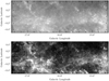 |
Fig. 19 Comparison of the Hi-GAL NH2 map (top) and the 2D (3D velocity-integrated) 12CO (3–2) COHRS map (bottom) of a portion of the Gp centred at (l, b) = 16°, 0°. |
8.3 Generalization capability of our models
To evaluate the generalization capability of our models, we performed a segmentation of the 2D (velocity-integrated) 12CO (3–2) COHRS map covering part of the Gp (see Section 7.2.1). The result of this generalization is presented in Section 7.2.7 and Figure 18. Results show that the use of the PE-UNet-1 model learnt on the normalized column density image of the Gp well reproduced the filamentary structures observed on the 2D COHRS map, confirming the generalization of it. Apart from the noisy regions associated with COHRS data where the model does not perform well in recovering the filamentary structures, the other regions are well detected.
Figure 19 shows the original data used in this experiment of generalization, the Hi-GAL column density map and the velocity-integrated COHRS map, both before their local min-max normalization. We note that despite being observed at different wavelengths, with different instruments and at different spatial resolutions and tracing not the same phases of the ISM, the two images show similar emission features, including filamentary structures and bright compact sources that are clearly noticeable. This experience shows that for data having a similar emission structure than the NH2 column density map, a reasonable result to detect filaments in the data can be obtained by applying the model learnt on NH2 data. This offers important perspectives for filament detection on large multi-wavelength surveys of the Gp, allowing the study of filament properties over a large range of physical conditions, from the cold ISM traced by H I to the warmer phases better traced in the infrared.
9 Conclusions
With the aim of proposing a robust method for filament detection over a large range of density and contrast observed in the Gp, we explored the interest of position encoding in supervised learning, following our proof-of-concept work (Zavagno et al. 2023). We presented an in-depth analysis of the existing segmentation methods to allow the better detection of filaments in the Gp, covering a large range in column density and contrast. We introduced the random k-fold for data distribution that allowed us to obtain, for the first time, a segmentation of the whole Gp with machine learning.
Starting from the Hi-GAL NH2 column density map of the Gp, we created a locally normalized column density map that reveals the high degree of filamentary structures of the Gp ISM over the whole covered range of column density. Using nearinfrared data from 2MASS, mid-infrared data from Spitzer, and COHRS spectroscopic data, we discuss the robustness of this normalized column density map that allowed us to ascertain the detected structures.
Compared to previous works, we introduced the encoding of the position of the patches in the Gp as an additional input to the network. We proposed three UNet models that take as input the patch and the position, which we call PE-UNet (Position encoding UNet), which differ by the way this latter additional information is input to the network.
We showed that exploiting the position in PE-UNets significantly improves the detection over classical segmentation architectures such as UNet, UNet++ and Swin-UNet. We further studied how the three PE-UNet variants behave and proposed explanations for the performance of the three models. We conclude that the PE-UNet is particularly sensitive to the contrast of the structures in the original column density map. We observe that the model PE-UNet-Latent, where the position encoding is input in the latent space of the model, allows better detection of both high-contrast and high-density structures (giving a better score on the segmented map). It is particularly well suited for detecting low-contrast structures that are barely detected (or not detected at all) by more standard UNet models.
We also applied our best-learnt model (using PE-UNet-L) to 2D 12CO (3–2) COHRS data and show that the model can be applied with reasonable results on a similar dataset. This generalization capability offers interesting perspectives for the model to be applied to large surveys of the Gp.
The detection of filaments over a wide range of density and contrast with PE-UNet-based models, possibly extended to different datasets with one learnt model, offers important perspectives for the analysis of filaments observed in the Gp, in particular to follow the life cycle of filaments (from their formation to their fragmentation and collapse to form stars).
Acknowledgements
The authors thank the support of the CNRS-Mission pour les Initiatives Transverses et Interdisciplinaires (MITI). AZ thanks the support of the Institut Universitaire de France (IUF). Software: Aladin (Bonnarel et al. 2000), APLpy (Robitaille & Bressert 2012; Robitaille 2019), astropy (Astropy Collaboration 2022), Matplotlib (Hunter 2007), NumPy (Harris et al. 2020), SciPy (Virtanen et al. 2020). This document was prepared using the Overleaf web application.
Appendix A Building balanced datasets
A.1 Random subsets generation
As discussed in Section 5.1.1 of the manuscript we need to build a series of training/validation/test datasets to enable inference over the full Gp. This requires care since the data must be divided into training/validation/test so that the distribution of training samples, validation samples and test samples are aligned. In our case, this means that one should take into the nature of patches (e.g. low vs high density and/or contrast) and the distribution of filament pixels which both vary with the longitude of the patch (for instance there are more filament pixels in the centre of the Gp than on the sides).
Hence we implemented a procedure to randomly create k subsets of the Gp which are balanced according to the longitude distribution. The Gp is first divided into a uniform grid of squared areas (we used areas of 64 × 64 pixels). Then we perform a partitioning of these areas in k subsets. For each longitude (i.e. column of areas; see figure A.1), starting from the left of the figure (centre of the Gp) to the right, the areas in the columns are distributed amongst the subsets from top to bottom. The top area (top of the figure) is randomly associated with one of the k subsets, say subseti. The next area (the one below) is associated with subseti+1, for example. The same random process is iterated over columns from left to right. This partitioning is illustrated in Figure A.1) for k = 3 and where the height of the Gp is about 6 areas. In this example, the first subset has been drawn for the first (left column), the third subset has been drawn for the second column, and so on. Following such a process ensures the areas in a subset are approximately balanced concerning their longitude. Once the subsets have been built, many (or all) patches are extracted (cropped) from all areas in a subset to build a set of samples (to be input to the segmentation models). To check the effect of our partitioning, we computed the longitude histogram within each subset and obtained approximately uniform distributions. The obtained histograms may be found in Figure A.1 for the case k = 5. One sees an inflexion point around 170°, which may be explained by the noisy regions around 170° which have been removed from the dataset (see Section 4.2).
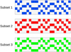 |
Fig. A.1 Balanced partitioning of the Galactic plane to segment the Hi-GAL dataset (Molinari et al. 2010; Schisano et al. 2020). The Gp is first divided into a number of areas (squared blocks in the plots). Then a partitioning of the Gp in k subsets is built where each subset gathers blocks that are uniformly distributed along the longitudinal axis (abscissas in the figure). In our experiments, we used blocks of 64 × 64 pixels as areas and many patches (samples) were extracted from every area. |
As explained in the manuscript k pairs of training/test sets are built from a set of subsets. To build one pair of datasets, one considers patches from all subsets but one in the training set (which will be again divided into training and validation data), and patches from the last subset in the test set.
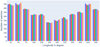 |
Fig. A.2 For each subset, the histogram of the number of patches is split as a function of the longitude (one colour per subset). The variability along the longitude axis is the result of noisy regions removed from the dataset. |
A.2 Random versus naive subsets generation
Alternatively, we could have used a simple, which we call naive, subset generation, which is illustrated in Figure A.3). A naive subset generation divides the Gp into k strips of equal size along the longitude axis (see Figure A.3). Training/validation/test datasets are then built as explained above.
Going back to our motivation for designing the random subset generation procedure we compare here such a naive subset generation with the proposed random subset generation in terms of the number of pixels labelled as filament and background in the k generated subsets.
 |
Fig. A.3 Band (naive) partitioning of the Galactic plane to segment the Hi-GAL dataset (Molinari et al. 2010; Schisano et al. 2020). The Gp is divided into k bands which constitute the testing datasets. Models are trained on the remaining data. From those bands, we extract many patches (samples) that compose the different datasets. |
We plot the number of pixels labelled as filament and background in every subset for the random subsets generation and for the naive subsets generation (using k = 10). As expected, the random generation produces balanced datasets with less than 0.7% difference between two subsets for both filament and background (see Figure A.4) while one can observe up to 13% difference between subsets generated by the naive procedure.
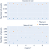 |
Fig. A.4 Number of pixels labelled as filament and background (y-axis) in each of the ten subsets (x-axis) built using the random procedure (top) and the naive procedure (bottom). |
Appendix B Position regression
Depending on the local physical conditions, the position of a filament in the Gp will influence its properties such as its orientation (driven by the magnetic field), density and star formation properties (depending on its evolutionary status and local physical conditions). Consequently, the position information should play a role in filament detection and help statistical-based methods such as neural networks.
While we propose in the paper to use the position of a patch as an additional input to help segmentation, one may ask whether the position information is not already available, to some extent, in the density patch itself. If this was the case one should be able to learn a model to predict the position of a patch within the Gp based on the normalized density map patch. To test this hypothesis, we used a model with the shape of the encoder of our UNet models (hence with a similar capacity as our segmentation models) with a few fully connected layers added on top. We learned the model to perform the regression task of predicting the latitude (or latitude encoding) and the longitude (or longitude encoding) of the patches. We performed experiments with and without data augmentation (rotations and flips). The best results were given when predicting position encoding without the use of data augmentation. The regression results of this specific experiment are presented in Figure B.1 where the predicted position distribution is represented on the y-axis against the ground-truth. A tendency to follow the red curve which represents the perfect regression solution (predict = true label) can be observed for the longitude axis even if the distributions within each band remain quite large. The latitude distributions present every sign of a close-to-random distribution. This indicates that part of the position information is contained and retrievable from the patch itself and therefore could be extracted by neural network to perform filament segmentation.
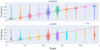 |
Fig. B.1 Violin plot of the predicted position encoding for longitude (top) and latitude (bottom) as a function of the ground truth. |
We now want to verify that the information is used during the segmentation task. To test this hypothesis, we take the encoder part of one UNet trained for the segmentation task during the cross-validation procedure described in Section 5.1.1 and add the same dense architecture used in the previous experiment to perform the regression task (position or position encoding prediction). We keep the exact same procedure and data for a fair comparison but we freeze the weight of the encoder part of the neural network, i.e. only the classification layers will be updated during the training phase, and the encoder part will remain unchanged. This allows us to check if we can extract the position information from the compressed representation of the data produced by the encoding part of the UNet when the targeted task is semantic segmentation. Results show that in every configuration (position or position encoding prediction and whether or not we use data augmentation) the position information is not contained in the embedding representation of the data. Despite the fact that our model converges during training, we observe poor performance in test (see Figure B.2). The loss of position information during segmentation training, while it is well accepted that position plays a role in filament properties and detection, motivates us to give it as input to our model in order for it to utilize this information (see Section 5.2).
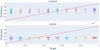 |
Fig. B.2 Violin plot of the predicted position encoding for longitude (top) and latitude (bottom) for every 0.1 position encoding. The x-axis corresponds to true labels while the y-axis displays the predicted value. The red curve represents the perfect regression solution (predict = true label). Both the latitude and longitude distributions present every sign of a close-to-random distribution. |
Appendix C Partially supervised learning
While Schisano et al. (2020) work is a rich dataset for supervised machine learning, we do not recommend training machine learning models directly on this dataset for two main reasons:
First, if a model is fed directly with Schisano et al. (2020) results as pixel annotation, it will at best mimic the Hessian method. While this could be a good option to aggregate the hessian and the post-processing (e.g. filtering small structures, removing artefacts) part of Schisano et al. (2020) work into one single model and remove the hyperparameter dependency, it won’t improve significantly performance, it cannot detect new structures that have been missed by the Hessian method.
Second, as good as Schisano et al. (2020) method is, it missed some structures and added some artefacts (some did not get removed during the post-processing phase). As deep learning model performance highly depend on the input data, we want to avoid training neural networks in noisy settings (some samples of the training dataset are labelled with one wrong label) because it reduces neural network performance as shown in Song et al. (2022); Krause et al. (2016); Arpit et al. (2017); Zhang et al. (2021).
To compensate for this and as done in Zavagno et al. (2023), we define (on the pixel level) the class filament by pixels annotated as such in Schisano et al. (2020) work. The class background is composed of pixels with intensity lower than conservative thresholds: for each mosaic, we determined a threshold for which pixels with lower intensity were with no doubt background (no filament). The remaining pixels are considered as unlabelled. To remove possible artifacts from the training data, we defined mosaic by mosaic areas where pixels would be considered as unlabelled, mainly located on the overlapping regions and the edge of the mosaics, the Hessian method being sensitive to edge effects. During training, every pixel will be fed into the network but the back-propagation will be done only on labelled pixels filament and background), i.e. the loss won’t be computed on unlabelled pixels. By using both background and filament-labelled pixels we want to prevent neural networks from overpredicting pixels as filaments. Machine learning models learn with equal importance to classify pixels as background or filament. Hence, predicting the class filament for a background pixel increases the training error (and the loss which learning aims at minimizing) and decreases performance metrics. When those pixels are considered, the dataset goes from a very unbalanced one (about 2% of pixels are labelled as filaments, the rest is labelled as background) to an almost balanced one (about 45% of pixels labelled as filaments and 55% as background).
Appendix D MSSIM
The MSSIM implementation used for performance measurement (see Section 7.1) can be found in Scikit-Image2 van der Walt et al. (2014). While Green et al. (2017) presents the MSSIM as a good metric for filament detection, we run some experiments to know how it behaves since it has no prior knowledge of what a filament is. It is an unsupervised metric and it depends on several hyperparameters which means results, hence conclusions, might depend on the hyperparameters used. If the MSSIM is a good metric to judge filament detection/segmentation quality, it should achieve two goals:
The MSSIM should get higher when we add real filaments to the detection, i.e. if we compute the MSSIM on one segmentation map and then on the same map but we add one true filament which was missing in the segmentation, the MSSIM should be higher for the second map because one true filament was added.
The MSSIM should get lower when we add a false filament to the detection, i.e., if we compute the MSSIM on one segmentation map and then on the same map but we add a false filament, the MSSIM of the second segmentation should be lower because there is one false filament added.
From those two statements, we design an experiment to check if they are verified or not:
Compute the MSSIM on a ground truth filament detection/segmentation.
Remove filaments one by one and compute the MSSIM over the whole map for each filament. Since those filaments are real (coming from a ground truth), the MSSIM should be lower for every map where one filament was removed.
For each exiting filament, add a copy to every space possible (without overlapping with existing filaments) and compute the MSSIM after each copy. Since this filament is false (we assume there is no missing filament in the ground truth), the MSSIM of the segmentation map and one added filament (wherever the filament is placed) should be lower than the ground truth one.
If the ground truth is complete and the MSSIM is a good metric, we should have 0% of true filaments increasing the MSSIM after being deleted and 0% of false filaments increasing the MSSIM after being added.
![Mathematical equation: $\[\operatorname{SSIM}(\mathrm{a}, \mathrm{b})=\frac{\left(2 \mu_{\mathrm{a}} \mu_{\mathrm{b}}+\mathrm{C}_{1}\right)\left(2 \sigma_{\mathrm{ab}}+\mathrm{C}_{2}\right)}{\left(\mu_{\mathrm{a}}^{2}+\mu_{\mathrm{b}}^{2}+\mathrm{C}_{1}\right)\left(\sigma_{\mathrm{a}}^{2}+\sigma_{\mathrm{b}}^{2}+\mathrm{C}_{2}\right)}\]$](/articles/aa/full_html/2024/12/aa50828-24/aa50828-24-eq20.png) (D.1)
(D.1)
In the MSSIM formula (see equation D.1), C1 and C2 are two hyperparameters to prevent instability caused by division by 0. We ran the above experiment for different values of C1 = C2 and as stated in Wang et al. (2004), it doesn’t have much influence on the results, as long as C1 << 1 and C2 << 1. In the Scikit-Image implementation of the MSSIM, there are two ways of computing it: either by block or with a Gaussian filter. The block method consists of simply computing the mean, variance, and covariance through a sliding window centre in each pixel of the image. The default window size is 7 pixels (this value has to be odd). The Gaussian method consists of applying a Gaussian filter before computing the mean, variance, and covariance through a sliding window. The window size is given by the hyper-parameter σ of the Gaussian filter by the following formula:
![Mathematical equation: $\[\text{windowsize} (\sigma)=2 \times(3.5 \times \sigma+0.5)+1\]$](/articles/aa/full_html/2024/12/aa50828-24/aa50828-24-eq21.png) (D.2)
(D.2)
The metric presented originally in Wang et al. (2004) corresponds to the Gaussian implementation with σ = 1.5. To run our experiment, we select two representative regions of the Gp, one with high density and one with low density to have representative samples of the column density encountered during segmentation. The high- and low-density regions correspond respectively to longitude 314° to 321° and 173° to 180°. Table D.1 presents results from the experiments explained above, Column 1 indicates if the region studied corresponds to high or low density, Column 2 to the computation mode of the MSSIM, Column 3 the window size, Column 4 the percentage of true filament which increase the MSSIM after being deleted and Column 5 the number of false filament added that increase the MSSIM. One can observe that both the Gaussian and Block with a window size of 7 perform the same. No filament from the groundtruth was deleted but many false filaments increased the MSSIM score for both low- and high-density regions. On the counterpart, the Block implementation with a wider window (33 pixels in our experiments) adds fewer false filaments for both high- and low-density regions. However, few true filaments (respectively 2% and 3% for high- and low-density regions) were deleted according to the MSSIM. Those results indicate that the MSSIM is not behaving exactly how we would like to and it may vary depending on what hyper-parameters are used, conclusions based on only this metric should not be drawn.
Pourcentage of true filaments deleted and false filament added which increases the MSSIM score.
Appendix E Segmentation of the whole Gp
Because of the dynamic density and local normalization, high overlap and averaging methods are needed to avoid striation and discontinuity caused by edge effects in the segmentation maps (see Figure E.1). To overcome this difficulty, we utilize the dataset creation method outlined in Appendix A.1, with some adjustments:
We introduce an overlap of 31 pixels (on both axes) between subset areas during the mask creation step of dataset creation.
We did not define a validation set, models are trained with optimal hyperparameters selected during the crossvalidation scheme.
The overlap between patches within subset areas is also set to 31 pixels on both axes for the test sets only. In the neural network community, this corresponds to a stride (displacement between two successive patches) of 1.
For the training sets, the overlap is set to 16 pixels to reduce computation costs, hence a stride of 16.
Because of the dataset construction, when aggregating the different test sets of the subsets, we obtain one patch centred around every pixel of the Gp, in other words, each pixel appears in 1024 patches (in test). From these datasets, the segmentation map of the complete Gp is produced by the following steps:
Segment each patch individually.
Average, with uniform weights, the segmentation outputs for each pixel to achieve smooth segmentation across the entire Gp image.
Binarize the segmentation map using a threshold value of 0.5
Filter out small structures (filament smaller than 16 pixels (Schisano et al. 2020)) to eliminate non-significant features (Schisano et al. 2020, see Appendix B).
This method produces a smooth and nice-looking segmentation of the Gp as observed in Figure E.1. To generate the maps outlined in Section 7.2, we use a value of k equal to 10 (resulting in the training of ten models). The training and segmentation together require approximately 72 hours (duration may vary depending on the architecture trained). While a stride of 1 will present the fewest discontinuities after the averaging of the segmentation patch, it comes at a high computation price. We note that a stride of N increases the number of patches by N2.
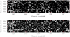 |
Fig. E.1 Segmentation map obtained with an overlap of 31 pixels between patches (top) and with a 0 overlap (bottom), resulting in discontinuity along structures and striation effect in the second case. |
References
- Alina, D., Ristorcelli, I., Montier, L., et al. 2019, MNRAS, 485, 2825 [Google Scholar]
- Alina, D., Shomanov, A., & Baimukhametova, S. 2022, IEEE Access, 10, 74472 [NASA ADS] [CrossRef] [Google Scholar]
- André, P., Men’shchikov, A., Bontemps, S., et al. 2010, A&A, 518, L102 [NASA ADS] [CrossRef] [EDP Sciences] [Google Scholar]
- André, P., Di Francesco, J., Ward-Thompson, D., et al. 2014, in Protostars and Planets VI, eds. H. Beuther, R. S. Klessen, C. P. Dullemond, & T. Henning, 27 [Google Scholar]
- Arpit, D., Jastrzębski, S., Ballas, N., et al. 2017, in International conference on machine learning, PMLR, 233 [Google Scholar]
- Arzoumanian, D., André, P., Didelon, P., et al. 2011, A&A, 529, L6 [NASA ADS] [CrossRef] [EDP Sciences] [Google Scholar]
- Arzoumanian, D., André, P., Könyves, V., et al. 2019, A&A, 621, A42 [NASA ADS] [CrossRef] [EDP Sciences] [Google Scholar]
- Arzoumanian, D., Russeil, D., Zavagno, A., et al. 2022, A&A, 660, A56 [NASA ADS] [CrossRef] [EDP Sciences] [Google Scholar]
- Asgari Taghanaki, S., Abhishek, K., Cohen, J. P., Cohen-Adad, J., & Hamarneh, G. 2021, Artif. Intell. Rev., 54, 137 [Google Scholar]
- Astropy Collaboration (Price-Whelan, A. M., et al.) 2022, ApJ, 935, 167 [NASA ADS] [CrossRef] [Google Scholar]
- Bekki, K. 2021, A&A, 647, A120 [NASA ADS] [CrossRef] [EDP Sciences] [Google Scholar]
- Benedettini, M., Schisano, E., Pezzuto, S., et al. 2015, MNRAS, 453, 2036 [NASA ADS] [CrossRef] [Google Scholar]
- Bešlić, I., Coudé, S., Lis, D. C., et al. 2024, A&A, 684, A212 [NASA ADS] [CrossRef] [EDP Sciences] [Google Scholar]
- Bianco, M., Giri, S. K., Iliev, I. T., & Mellema, G. 2021, MNRAS, 505, 3982 [NASA ADS] [CrossRef] [Google Scholar]
- Bonnarel, F., Fernique, P., Bienaymé, O., et al. 2000, A&AS, 143, 33 [NASA ADS] [CrossRef] [EDP Sciences] [Google Scholar]
- Bui, T. D., Wang, L., Chen, J., et al. 2019, in Domain Adaptation and Representation Transfer and Medical Image Learning with Less Labels and Imperfect Data: First MICCAI Workshop, DART 2019, and First International Workshop, MIL3ID 2019, Shenzhen, Held in Conjunction with MICCAI 2019, Shenzhen, China, October 13 and 17, 2019, Proceedings 1, Springer, 243–251 [Google Scholar]
- Cao, H., Wang, Y., Chen, J., et al. 2023, in Computer Vision – ECCV 2022 Workshops, eds. L. Karlinsky, T. Michaeli, & K. Nishino (Cham: Springer Nature Switzerland), 205 [Google Scholar]
- Carrière, J.-S., Ferrière, K., Ristorcelli, I., & Montier, L. 2022a, A&A, 668, A42 [NASA ADS] [CrossRef] [EDP Sciences] [Google Scholar]
- Carrière, J.-S., Montier, L., Ferrière, K., & Ristorcelli, I. 2022b, A&A, 668, A41 [NASA ADS] [CrossRef] [EDP Sciences] [Google Scholar]
- Chen, Y.-C., Genovese, C. R., & Wasserman, L. 2014, arXiv e-prints [arXiv:1406.1803] [Google Scholar]
- Chen, Y.-C., Ho, S., Tenneti, A., et al. 2015, MNRAS, 454, 3341 [NASA ADS] [CrossRef] [Google Scholar]
- Chen, M. C.-Y., Di Francesco, J., Rosolowsky, E., et al. 2020, ApJ, 891, 84 [NASA ADS] [CrossRef] [Google Scholar]
- Clark, S., & Hensley, B. S. 2019, ApJ, 887, 136 [NASA ADS] [CrossRef] [Google Scholar]
- Clark, S., Peek, J., & Putman, M. 2014, ApJ, 789, 82 [NASA ADS] [CrossRef] [Google Scholar]
- Clark, S. E., Hill, J. C., Peek, J. E., Putman, M. E., & Babler, B. L. 2015, Phys. Rev. Lett., 115, 241302 [NASA ADS] [CrossRef] [Google Scholar]
- Clarke, S. D., Williams, G. M., & Walch, S. 2020, MNRAS, 497, 4390 [NASA ADS] [CrossRef] [Google Scholar]
- Cox, N., Arzoumanian, D., André, P., et al. 2016, A&A, 590, A110 [NASA ADS] [CrossRef] [EDP Sciences] [Google Scholar]
- Dewangan, L. K., Bhadari, N. K., Maity, A. K., et al. 2024, MNRAS, 527, 5895 [Google Scholar]
- Dib, S., Bontemps, S., Schneider, N., et al. 2020, A&A, 642, A177 [NASA ADS] [CrossRef] [EDP Sciences] [Google Scholar]
- Dosovitskiy, A., Beyer, L., Kolesnikov, A., et al. 2020, arXiv e-prints [arXiv:2010.11929] [Google Scholar]
- Elia, D., Molinari, S., Fukui, Y., et al. 2013, ApJ, 772, 45 [NASA ADS] [CrossRef] [Google Scholar]
- Feng, J., Smith, R. J., Hacar, A., Clark, S. E., & Seifried, D. 2024, MNRAS, 528, 6370 [NASA ADS] [CrossRef] [Google Scholar]
- Fiorellino, E., Elia, D., André, P., et al. 2021, MNRAS, 500, 4257 [Google Scholar]
- Frangi, A. F., Niessen, W. J., Vincken, K. L., & Viergever, M. A. 1998, in Medical Image Computing and Computer-Assisted Intervention – MICCAI’98: First International Conference Cambridge, MA, USA, October 11–13, 1998 Proceedings 1 (Springer), 130 [Google Scholar]
- Fu, K.-S., & Mui, J. 1981, Pattern Recogn., 13, 3 [NASA ADS] [CrossRef] [Google Scholar]
- Goodfellow, I., Bengio, Y., & Courville, A. 2016, Deep Learning (MIT Press) [Google Scholar]
- Green, C.-E., Cunningham, M. R., Dawson, J. R., et al. 2017, ApJ, 840, L17 [NASA ADS] [CrossRef] [Google Scholar]
- Hacar, A., Tafalla, M., Forbrich, J., et al. 2018, A&A, 610, A77 [NASA ADS] [CrossRef] [EDP Sciences] [Google Scholar]
- Hacar, A., Clark, S., Heitsch, F., et al. 2023, in Astronomical Society of the Pacific Conference Series, 534, 153 [NASA ADS] [Google Scholar]
- Hacar, A., Clark, S. E., Heitsch, F., et al. 2023, in Protostars and Planets VII, eds. S. Inutsuka, Y. Aikawa, T. Muto, K. Tomida, & M. Tamura, Astronomical Society of the Pacific Conference Series, 534, 153 [NASA ADS] [Google Scholar]
- Harris, C. R., Millman, K. J., van der Walt, S. J., et al. 2020, Nature, 585, 357 [NASA ADS] [CrossRef] [Google Scholar]
- Hausen, R., & Robertson, B. E. 2020, ApJS, 248, 20 [CrossRef] [Google Scholar]
- He, H., & Ma, Y. 2013, Imbalanced learning: foundations, algorithms, and applications (John Wiley & Sons) [CrossRef] [Google Scholar]
- He, K., Zhang, X., Ren, S., & Sun, J. 2016, in Proceedings of the IEEE Conference on Computer Vision and Pattern Recognition, 770 [Google Scholar]
- Hoemann, E., Heigl, S., & Burkert, A. 2021, MNRAS, 507, 3486 [NASA ADS] [CrossRef] [Google Scholar]
- Hsieh, C.-H., Arce, H. G., Mardones, D., Kong, S., & Plunkett, A. 2021, ApJ, 908, 92 [CrossRef] [Google Scholar]
- Huang, H., Lin, L., Tong, R., et al. 2020, in ICASSP 2020–2020 IEEE International Conference on Acoustics, Speech and Signal Processing (ICASSP), IEEE, 1055 [Google Scholar]
- Huang, S.-Y., Hsu, W.-L., Hsu, R.-J., & Liu, D.-W. 2022, Diagnostics, 12 [Google Scholar]
- Hunter, J. D. 2007, Comput. Sci. Eng., 9, 90 [NASA ADS] [CrossRef] [Google Scholar]
- Izumi, N., Sanhueza, P., Koch, P. M., et al. 2024, ApJ, 963, 163 [NASA ADS] [CrossRef] [Google Scholar]
- Jégou, S., Drozdzal, M., Vazquez, D., Romero, A., & Bengio, Y. 2017, in Proceedings of the IEEE Conference on Computer Vision and Pattern Recognition Workshops, 11 [Google Scholar]
- Jetley, S., Lord, N. A., Lee, N., & Torr, P. H. 2018, arXiv e-prints [arXiv:1804.02391] [Google Scholar]
- Juvela, M. 2016, A&A, 593, A58 [NASA ADS] [CrossRef] [EDP Sciences] [Google Scholar]
- Kingma, D. P., & Ba, J. 2014, arXiv e-prints [arXiv:1412.6980] [Google Scholar]
- Koch, E. W., & Rosolowsky, E. W. 2015, MNRAS, 452, 3435 [Google Scholar]
- Könyves, V., André, P., Arzoumanian, D., et al. 2020, A&A, 635, A34 [Google Scholar]
- Krause, J., Sapp, B., Howard, A., et al. 2016, in Computer Vision – ECCV 2016: 14th European Conference, Amsterdam, The Netherlands, October 11–14, 2016, Proceedings, Part III 14 (Springer), 301 [Google Scholar]
- Krizhevsky, A., Sutskever, I., & Hinton, G. E. 2017, Commun. ACM, 60, 84 [CrossRef] [Google Scholar]
- Kumar, M. S. N., Palmeirim, P., Arzoumanian, D., & Inutsuka, S. I. 2020, A&A, 642, A87 [EDP Sciences] [Google Scholar]
- Kumar, M. S. N., Arzoumanian, D., Men’shchikov, A., et al. 2022, A&A, 658, A114 [NASA ADS] [CrossRef] [EDP Sciences] [Google Scholar]
- LeCun, Y., Boser, B., Denker, J., et al. 1989, Adv. Neural Inform. Process. Syst., 2 [Google Scholar]
- Li, Z. 2023, Highlights Sci. Eng. Technol., 39, 1245 [CrossRef] [Google Scholar]
- Li Causi, G., Schisano, E., Liu, S. J., Molinari, S., & Di Giorgio, A. 2016, SPIE Conf. Ser., 9904, 99045V [NASA ADS] [Google Scholar]
- Linardatos, P., Papastefanopoulos, V., & Kotsiantis, S. 2020, Entropy, 23, 18 [NASA ADS] [CrossRef] [Google Scholar]
- Liu, B., & Liu, J. 2019, J. Phys. Conf. Ser., 1176, 022010 [NASA ADS] [CrossRef] [Google Scholar]
- Liu, Z., Lin, Y., Cao, Y., et al. 2021, in Proceedings of the IEEE/CVF International Conference on Computer Vision, 10012 [Google Scholar]
- Maity, A. K., Dewangan, L. K., Bhadari, N. K., et al. 2023, MNRAS, 523, 5388 [NASA ADS] [CrossRef] [Google Scholar]
- Malinen, J., Montier, L., Montillaud, J., et al. 2016, MNRAS, 460, 1934 [Google Scholar]
- Mattern, M., Kauffmann, J., Csengeri, T., et al. 2018, A&A, 619, A166 [NASA ADS] [CrossRef] [EDP Sciences] [Google Scholar]
- Men’shchikov, A. 2013, A&A, 560, A63 [Google Scholar]
- Men’shchikov, A. 2021, A&A, 649, A89 [EDP Sciences] [Google Scholar]
- Molinari, S., Swinyard, B., Bally, J., et al. 2010, A&A, 518, L100 [NASA ADS] [CrossRef] [EDP Sciences] [Google Scholar]
- Molinari, S., Schisano, E., Elia, D., et al. 2016, A&A, 591, A149 [NASA ADS] [CrossRef] [EDP Sciences] [Google Scholar]
- Motte, F., Bontemps, S., Csengeri, T., et al. 2022, A&A, 662, A8 [NASA ADS] [CrossRef] [EDP Sciences] [Google Scholar]
- Oktay, O., Schlemper, J., Folgoc, L. L., et al. 2018, arXiv e-prints [arXiv:1804.03999] [Google Scholar]
- Ossenkopf-Okada, V., & Stepanov, R. 2019, A&A, 621, A5 [NASA ADS] [CrossRef] [EDP Sciences] [Google Scholar]
- Palmeirim, P. a., André, P., Kirk, J., et al. 2013, A&A, 550, A38 [NASA ADS] [CrossRef] [EDP Sciences] [Google Scholar]
- Panopoulou, G. V., Tassis, K., Goldsmith, P., & Heyer, M. 2014, MNRAS, 444, 2507 [NASA ADS] [CrossRef] [Google Scholar]
- Panopoulou, G., Psaradaki, I., & Tassis, K. 2016, MNRAS, 462, 1517 [Google Scholar]
- Panopoulou, G., Psaradaki, I., Skalidis, R., Tassis, K., & Andrews, J. 2017, MNRAS, 466, 2529 [NASA ADS] [CrossRef] [Google Scholar]
- Park, G., Currie, M. J., Thomas, H. S., et al. 2023, ApJS, 264, 16 [NASA ADS] [CrossRef] [Google Scholar]
- Peretto, N., & Fuller, G. A. 2009, A&A, 505, 405 [NASA ADS] [CrossRef] [EDP Sciences] [Google Scholar]
- Peretto, N., André, P., Könyves, V., et al. 2012, A&A, 541, A63 [NASA ADS] [CrossRef] [EDP Sciences] [Google Scholar]
- Pezzuto, S., Benedettini, M., Di Francesco, J., et al. 2021, A&A, 645, A55 [EDP Sciences] [Google Scholar]
- Pilbratt, G. L., Riedinger, J. R., Passvogel, T., et al. 2010, A&A, 518, L1 [NASA ADS] [CrossRef] [EDP Sciences] [Google Scholar]
- Pillai, T., Wyrowski, F., Menten, K. M., & Krügel, E. 2006, A&A, 447, 929 [NASA ADS] [CrossRef] [EDP Sciences] [Google Scholar]
- Pillsworth, R., & Pudritz, R. E. 2024, MNRAS, 528, 209 [NASA ADS] [CrossRef] [Google Scholar]
- Pineda, J. E., Arzoumanian, D., André, P., et al. 2022, arXiv e-prints [arXiv:2205.03935] [Google Scholar]
- Planck Collaboration Int. XXXII. 2016, A&A, 586, A135 [NASA ADS] [CrossRef] [EDP Sciences] [Google Scholar]
- Polychroni, D., Schisano, E., Elia, D., et al. 2013, ApJ, 777, L33 [CrossRef] [Google Scholar]
- Pouteau, Y., Motte, F., Nony, T., et al. 2022, A&A, 664, A26 [NASA ADS] [CrossRef] [EDP Sciences] [Google Scholar]
- Priestley, F., & Whitworth, A. 2022, MNRAS, 512, 1407 [NASA ADS] [CrossRef] [Google Scholar]
- Reyes-Reyes, S. D., Stutz, A. M., Megeath, S. T., et al. 2024, MNRAS, 529, 2220 [NASA ADS] [CrossRef] [Google Scholar]
- Rigby, A. J., Peretto, N., Anderson, M., et al. 2024, MNRAS, 528, 1172 [NASA ADS] [CrossRef] [Google Scholar]
- Rivera-Ingraham, A., Ristorcelli, I., Juvela, M., et al. 2016, A&A, 591, A90 [NASA ADS] [CrossRef] [EDP Sciences] [Google Scholar]
- Rivera-Ingraham, A., Ristorcelli, I., Juvela, M., et al. 2017, A&A, 601, A94 [NASA ADS] [CrossRef] [EDP Sciences] [Google Scholar]
- Robitaille, T. 2019, APLpy v2.0: The Astronomical Plotting Library in Python [Google Scholar]
- Robitaille, T., & Bressert, E. 2012, APLpy: Astronomical Plotting Library in Python, Astrophysics Source Code Library [record ascl:1208.017] [Google Scholar]
- Robitaille, J.-F., Motte, F., Schneider, N., Elia, D., & Bontemps, S. 2019, A&A, 628, A33 [NASA ADS] [CrossRef] [EDP Sciences] [Google Scholar]
- Ronneberger, O., Fischer, P., & Brox, T. 2015, in International Conference on Medical Image Computing and Computer-assisted Intervention (Springer), 234 [Google Scholar]
- Salji, C., Richer, J., Buckle, J., et al. 2015a, MNRAS, 449, 1782 [NASA ADS] [CrossRef] [Google Scholar]
- Salji, C., Richer, J. S., Buckle, J. V., et al. 2015b, MNRAS, 449, 1769 [NASA ADS] [CrossRef] [Google Scholar]
- Schisano, E., Rygl, K. L. J., Molinari, S., et al. 2014, ApJ, 791, 27 [Google Scholar]
- Schisano, E., Molinari, S., Elia, D., et al. 2020, MNRAS, 492, 5420 [Google Scholar]
- Shimajiri, Y., André, P., Ntormousi, E., et al. 2019, A&A, 632, A83 [NASA ADS] [CrossRef] [EDP Sciences] [Google Scholar]
- Skrutskie, M. F., Cutri, R. M., Stiening, R., et al. 2006, AJ, 131, 1163 [NASA ADS] [CrossRef] [Google Scholar]
- Soler, J. D., Hennebelle, P., Martin, P., et al. 2013, ApJ, 774, 128 [NASA ADS] [CrossRef] [Google Scholar]
- Soler, J. D., Miville-Deschênes, M. A., Molinari, S., et al. 2022, A&A, 662, A96 [NASA ADS] [CrossRef] [EDP Sciences] [Google Scholar]
- Song, H., Kim, M., Park, D., Shin, Y., & Lee, J.-G. 2022, IEEE Transactions on Neural Networks and Learning Systems [Google Scholar]
- Sousbie, T. 2011, MNRAS, 414, 350 [NASA ADS] [CrossRef] [Google Scholar]
- Thoma, M. 2016, CoRR, arXiv e-prints [1602.06541] [Google Scholar]
- Torpmann-Hagen, B., Thambawita, V., Glette, K., Halvorsen, P., & Riegler, M. A. 2022, Segmentation Consistency Training: Out-of-Distribution Generalization for Medical Image Segmentation [Google Scholar]
- van der Walt, S., Schönberger, J. L., Nunez-Iglesias, J., et al. 2014, PeerJ, 2, e453 [Google Scholar]
- Virtanen, P., Gommers, R., Oliphant, T. E., et al. 2020, Nature Methods, 17, 261 [CrossRef] [Google Scholar]
- Vojtekova, A., Lieu, M., Valtchanov, I., et al. 2021, MNRAS, 503, 3204 [Google Scholar]
- Wang, K., Zhang, Q., Testi, L., et al. 2014, MNRAS, 439, 3275 [Google Scholar]
- Wang, Z., Bovik, A., Sheikh, H., & Simoncelli, E. 2004, IEEE Trans. Image Process., 13, 600 [CrossRef] [Google Scholar]
- Whitney, B., Benjamin, R., Meade, M., et al. 2011, in American Astronomical Society Meeting Abstracts, 217, 241.16 [NASA ADS] [Google Scholar]
- Xu, D., Kong, S., Kaul, A., Arce, H. G., & Ossenkopf-Okada, V. 2023a, ApJ, 955, 113 [NASA ADS] [CrossRef] [Google Scholar]
- Xu, F.-W., Wang, K., Liu, T., et al. 2023b, MNRAS, 520, 3259 [NASA ADS] [CrossRef] [Google Scholar]
- Yuen, K. K., & Dixon, W. J. 1973, Biometrika, 60, 369 [CrossRef] [Google Scholar]
- Zavagno, A., André, P., Schuller, F., et al. 2020, A&A, 638, A7 [NASA ADS] [CrossRef] [EDP Sciences] [Google Scholar]
- Zavagno, A., Dupé, F. X., Bensaid, S., et al. 2023, A&A, 669, A120 [NASA ADS] [CrossRef] [EDP Sciences] [Google Scholar]
- Zhang, Z., Liu, Q., & Wang, Y. 2018, IEEE Geosci. Remote Sens. Lett., 15, 749 [CrossRef] [Google Scholar]
- Zhang, C., Bengio, S., Hardt, M., Recht, B., & Vinyals, O. 2021, Commun. ACM, 64, 107 [CrossRef] [Google Scholar]
- Zhou, Z., Siddiquee, M. M. R., Tajbakhsh, N., & Liang, J. 2019, IEEE Trans. Med. Imaging, 39, 1856 [Google Scholar]
- Zhu, X.-P., Dai, J.-M., Bian, C.-J., et al. 2019, Astrophys. Space Sci., 364, 55 [NASA ADS] [CrossRef] [Google Scholar]
All Tables
Pourcentage of true filaments deleted and false filament added which increases the MSSIM score.
All Figures
|
Fig. 1 Simplified UNet architecture (Ronneberger et al. 2015). The complete architecture is composed of 5 UNet blocks (here only three are represented). A UNet block is composed of two convolutions 3 × 3 and Relu activation followed by a max pooling layer for the encoding part and one up-convolution layer followed by two convolutions 3 × 3 and Relu activation for the decoding part. Skip connections correspond to the concatenation operation and are represented by dashed lines. With our implementation (five blocks), we obtain an output of size 2 × 2 × 1024 after the bottleneck given an image of size 32 × 32 × 1. The input image is represented on the left, while the output is shown on the right. |
| In the text | |
|
Fig. 2 Filament distribution along the longitude (top) and latitude (bottom) axis of the Galactic plane, from the catalogue of candidate filaments published in Schisano et al. (2020). The Galactic centre is located at (0°, 0°) (for the longitude, 0° corresponds to 360°). The bandwidth used to compute histograms is 1000 pixels for longitude and 50 for latitude. |
| In the text | |
|
Fig. 3 Concatenation operation. We add position information as two additional channels or maps to the existing one already through a concatenation operation. The existing channels or maps can be either the density input or the results from a convolution layer (h and w being the channel or map size). We fill a h × w matrix with the position encoding pl. |
| In the text | |
|
Fig. 4 Position Encoding UNet architecture. The model consists of a UNet architecture with the patch position as an additional input. Three alternatives of PE-UNet have been explored, Input (in orange), where we input the position as two additional channels before the first layer; Latent (in green), where we input the position as two additional features after the bottleneck; Decision (in red), where we input the position as two additional features before the last convolution. In our experiment, the PE-UNets are composed of five UNet blocks reducing the dimension to 2 × 2 × 1024 at the bottleneck level given a patch of size 32 × 32 × 1. |
| In the text | |
|
Fig. 5 Comparison of the column density map (top) and the corresponding local normalized column density image (bottom) on a low-density region of the Gp centred at (l, b) = 181°, 0°. Examples of high- and low-contrast filaments (discussed in the text) present on the original column density map (top) and their counterparts on the normalized map (bottom) are identified with cyan and yellow arrows, respectively. The red square (top) shows a 32 × 32 pixels box over which the normalization is performed. The original column density map is represented in logarithmic scale and spans the range 1 × 10²¹ to 2 × 1022 cm−2. |
| In the text | |
|
Fig. 6 Comparison of the column density map (top) and the corresponding local normalized column density image (bottom) on a high-density region of the Gp centred at (l, b) = 332°, 0°. Examples of high- and low-contrast filaments (see text) present on the original column density map (top) and their counterparts on the normalized map (bottom) are identified with cyan and yellow arrows, respectively. The original column density map is represented in logarithmic scale and spans the range 6 × 10²¹ to 1 × 1023 cm−2. The white and black squares on the original column density and normalized map, respectively, are saturated regions. |
| In the text | |
|
Fig. 7 Comparison of the COHRS 12CO (3—2) velocity-integrated image (top) and the corresponding local normalized column density image (bottom) on a low-density region of the Gp centred at (l, b) = 16.5°, 0°. The compact sources (red circles) and filamentary structures (orange arrows) seen on the two maps are underlined. The COHRS image is represented in a linear scale with an intensity that spans the range of 0–80 K km/s. |
| In the text | |
|
Fig. 8 Comparison of the 2MASS JHKS colour image (top left), normalized column density map (top right), column density map (bottom left) and COHRS 12CO (3–2) velocity-integrated image (bottom right) in a low-density region of the Gp centred at (l, b) = 16°, 0°. The original column density is displayed in logarithmic scale and spans the range 3 × 10²¹ to 5 × 1022 cm−2. The COHRS image is represented in a linear scale with an intensity that spans the range of 0–70 K km/s. |
| In the text | |
|
Fig. 9 Comparison of GLIMPSE 3603.6 μm (orange) and 4.5 μm (red) Spitzer-IRAC image (top left), the normalized column density map (top right), the column density map (bottom left) and the COHRS 12CO (3–2) velocity-integrated image (bottom right) in a region of the Gp centred at (l, b) =10.50°, −0.18°. Weote the presence of the infrared dark cloud G11.11–0.12, the Galactic ‘Snake’, identified by the red arrow. The original column density is displayed logarithmic scale and spans the range 1 × 10²¹ to 1 × 1023 cm−2. The COHRS image is represented in a linear scale with intensity that spans the range of 0–100 K km/s. |
| In the text | |
|
Fig. 10 Comparison of the segmented maps obtained using the PE-UNet-L and UNet versions centred on a low column density region of the plane at the location around l = 163°, 0°. The difference between the two segmented maps (PE-UNet-L – UNet) is shown (left) with the corresponding column density map (middle) and local normalized column density map (right). The white (black) features seen on the left map correspond to features detected with the PE-UNet-L (UNet) only. |
| In the text | |
|
Fig. 11 Comparison of the segmented maps obtained using the PE-UNet-L and UNet versions centred on a high column density region of the plane at the location around (l, b) = 353°, 0°. The difference between the results of the two segmented maps (PE-UNet-L – UNet) is shown (left) with the corresponding column density map (middle) and the local normalized column density map (right). The white (black) features seen on the left map correspond to features detected with the PE-UNet-L (UNet) only. |
| In the text | |
|
Fig. 12 Comparison of the segmented maps obtained using the PE-UNet-L and UNet versions centred on a high column density region of the plane at the location around (l, b) = 144°, 0.3°. The difference between the result of the two segmented maps (PE-UNet-L – UNet) is shown (left) with the corresponding column density map (middle) and the local normalized column density map (right). The white features seen on the left map correspond to features detected only with the PE-UNet-L. |
| In the text | |
|
Fig. 13 Comparison of the segmented maps obtained using the PE-UNet-L and UNet at location around (l, b) = 305°, 0°. The difference between the binarized PE-UNet-L and UNet segmentation maps (top), the normalized column density map (middle), and the original column density map (bottom) are shown. The white (black) features seen on the top map correspond to features detected with the PE-UNet-L (UNet) only. |
| In the text | |
|
Fig. 14 Comparison of the segmented map obtained using (from top to bottom) the PE-UNet-L and the original input mask map detected by Schisano et al. (2020) at the location around (l, b) = 180°, 0°. The original and normalized column density maps are also shown. |
| In the text | |
|
Fig. 15 Comparison of the segmented map (from top to bottom) obtained using the PE-UNet-L and the original input mask map detected by Schisano et al. (2020) at the location around (l, b) = 308°, 0°. The original and normalized column density maps are also shown. |
| In the text | |
|
Fig. 16 Comparison of the segmented maps (from top to bottom) obtained using the three PE-UNet versions at the low-density location centred on (l, b) = 180°, 0°: PE-UNet-I, PE-UNet-D, PE-UNet-L. The corresponding normalized column density map is also shown. |
| In the text | |
|
Fig. 17 Comparison of the segmented maps obtained using the three PE-UNet versions at the dense location centred on (l, b) = 308°, 0° (from top to bottom): PE-UNet-I, PE-UNet-D, PE-UNet-L. The corresponding normalized column density map is also shown (bottom). |
| In the text | |
|
Fig. 18 Segmentation of the velocity-integrated 2D (position, position) 12 CO (3–2) COHRS map using the model learnt on the column density image of the Gp with PE-UNet-L at the location centred at (l, b) = 16.5°, 0°. The min–max normalized COHRS (top left) and NH2 (top right) maps are shown. The corresponding segmented maps using the PE-UNet-L learnt model on NH2 data are shown for COHRS (bottom left) and NH2 (bottom right). |
| In the text | |
|
Fig. 19 Comparison of the Hi-GAL NH2 map (top) and the 2D (3D velocity-integrated) 12CO (3–2) COHRS map (bottom) of a portion of the Gp centred at (l, b) = 16°, 0°. |
| In the text | |
|
Fig. A.1 Balanced partitioning of the Galactic plane to segment the Hi-GAL dataset (Molinari et al. 2010; Schisano et al. 2020). The Gp is first divided into a number of areas (squared blocks in the plots). Then a partitioning of the Gp in k subsets is built where each subset gathers blocks that are uniformly distributed along the longitudinal axis (abscissas in the figure). In our experiments, we used blocks of 64 × 64 pixels as areas and many patches (samples) were extracted from every area. |
| In the text | |
|
Fig. A.2 For each subset, the histogram of the number of patches is split as a function of the longitude (one colour per subset). The variability along the longitude axis is the result of noisy regions removed from the dataset. |
| In the text | |
|
Fig. A.3 Band (naive) partitioning of the Galactic plane to segment the Hi-GAL dataset (Molinari et al. 2010; Schisano et al. 2020). The Gp is divided into k bands which constitute the testing datasets. Models are trained on the remaining data. From those bands, we extract many patches (samples) that compose the different datasets. |
| In the text | |
|
Fig. A.4 Number of pixels labelled as filament and background (y-axis) in each of the ten subsets (x-axis) built using the random procedure (top) and the naive procedure (bottom). |
| In the text | |
|
Fig. B.1 Violin plot of the predicted position encoding for longitude (top) and latitude (bottom) as a function of the ground truth. |
| In the text | |
|
Fig. B.2 Violin plot of the predicted position encoding for longitude (top) and latitude (bottom) for every 0.1 position encoding. The x-axis corresponds to true labels while the y-axis displays the predicted value. The red curve represents the perfect regression solution (predict = true label). Both the latitude and longitude distributions present every sign of a close-to-random distribution. |
| In the text | |
|
Fig. E.1 Segmentation map obtained with an overlap of 31 pixels between patches (top) and with a 0 overlap (bottom), resulting in discontinuity along structures and striation effect in the second case. |
| In the text | |
Current usage metrics show cumulative count of Article Views (full-text article views including HTML views, PDF and ePub downloads, according to the available data) and Abstracts Views on Vision4Press platform.
Data correspond to usage on the plateform after 2015. The current usage metrics is available 48-96 hours after online publication and is updated daily on week days.
Initial download of the metrics may take a while.