© The Authors 2024

1 Introduction

Models of dust coagulation in protoplanetary disks are required to understand the formation of cm-sized pebbles (Brauer et al. 2008; Birnstiel et al. 2009) and km-sized planetesimals (Wetherill & Stewart 1989; Schlichting & Sari 2011; Kobayashi et al. 2016; Lau et al. 2022; Drążkowska et al. 2023); they are indispensable for the interpretation of observational data (Birnstiel et al. 2018; Dullemond et al. 2018) and necessary to simulate the assembly of whole planetary systems (Lichtenberg et al. 2021; Emsenhuber et al. 2021). The size of dust grains also determines their aerodynamic properties and thus sets the timescales at which grains drift towards the central star or collect in local pressure maxima (Whipple 1972; Weidenschilling 1977). Furthermore, dust is the dominating source of opacity in circumstellar disks, which means the size distribution of the dust grains has a strong influence on the disks’ thermal structure (Muley et al. 2023) and hydrodynamics (Lesur et al. 2023), as well as on the interpretation of observations (Birnstiel et al. 2018; Leiendecker et al. 2022; Bergez-Casalou et al. 2022; Antonellini et al. 2023). In addition, the presence of small grains sets limits to the disks’ ionization and is thus also important for studies of magnetohydrodynamic mechanisms like the MRI (Balbus & Hawley 1991) and magnetized disk winds (Blandford & Payne 1982) with non-ideal MHD effects (Guillet et al. 2020; Pascucci et al. 2023; Tsukamoto & Okuzumi 2022). In 2018, observation with the Atacama Large Millimeter/submillimeter Array (ALMA) revealed that a broad variety of substructures exist in the spatial distribution of dust in protoplanetary disks (Andrews et al. 2018). Numerous gaps, spirals, and vortices have since been observed in the dust continuum emission (e.g., Pérez et al. 2018; Baruteau et al. 2019; Tsukagoshi et al. 2022) and also in molecular line observations (see Öberg et al. 2021). The existence of these structures raises questions regarding their origins and how they impact the formation and composition of planetesimals and planets within the disks – which makes hydrodynamic simulations of protoplanetary disks, including dust coagulation models, necessary (Birnstiel et al. 2018; Drążkowska et al. 2019).

Modeling the evolution of the solid content of protoplanetary disks has proven to be an expensive task in computational astrophysics. Many dust evolution models (e.g. Nakagawa et al. 1981; Weidenschilling 1980; Brauer et al. 2008; Birnstiel et al. 2010; Charnoz & Taillifet 2012; Drążkowska et al. 2019), numerically solve a discretized form of the Smoluchowski coagulation equation (Smoluchowski 1916). The coagulation equation’s integrodifferential nature makes solving it, however, numerically costly. This procedure utilizes a grid of grain sizes, meaning that dozens or hundreds of dust fluids have to be modeled in a single simulation, each representing grains of a different size that interact with every other grain size via collisions. Studies of dust coagulation are often carried out in one-dimensional disk models in either the radial direction (e.g., Lenz et al. 2020; Drążkowska et al. 2021; Pinilla et al. 2021; Gárate et al. 2021; Burn et al. 2022), the vertical direction (e.g, Zsom et al. 2011; Krijt & Ciesla 2016), or limited two-dimensional studies (Drążkowska et al. 2019).

Therefore, efforts are pursued to solve the coagulation equations more efficiently, such as the use of new numerical methods (e.g., Estrada & Cuzzi 2008; Lombart & Laibe 2021; Lombart et al. 2022, 2024; Marchand et al. 2021, 2022, 2023), or by applying far-reaching simplifications to the physics of dust coagulation (Birnstiel et al. 2012) that make it possible to implement dust coagulation as a subgrid model in hydrodynamic simulations (Tamfal et al. 2018; Vorobyov et al. 2018). Machine-learning- aided techniques also promise a fast, yet simplified approach to model dust coagulation on top of a hydrodynamic simulation (Pfeil et al. 2022).

Here, we present a semi-analytic model of dust coagulation, which is based on a two-population approach, originally developed by (Birnstiel et al. 2012) and employed in various forms by others (Tamfal et al. 2018; Vorobyov et al. 2019, 2020; Vorobyov & Elbakyan 2019). This model, however, has the critical disadvantage of not evolving the full dust size distribution but only the maximum particle size. With our new model, we are now able to conduct two-dimensional, vertically integrated hydrodynamics simulations of protoplanetary disks with an evolving dust size distribution at low computational cost. Figure 1 shows an example comparison between a full coagulation simulation, conducted with DustPy (Stammler & Birnstiel 2022) – a full-fledged dust coagulation software – and a one-dimensional hydrodynamic simulation with the PLUTO code equipped with our new method. While one-dimensional hydrodynamics simulations do not allow for a direct comparison of performance due to the different methods to handle the transport (DustPy utilizes an implicit integration scheme and does not solve the equations of hydrodynamics, but an advection-diffusion equation for a Keplerian disk), they allow for detailed tests of the accuracy of our new model.

This article is structured as follows: in Section 2, we briefly review the physics of dust dynamics and coagulation. We also give a short description of two-pop-py (Birnstiel et al. 2012), the progenitor of our new model. Section 3 introduces our new three-parameter dust coagulation model TriPoD and how it is integrated in the PLUTO hydrodynamics code (Mignone et al. 2007). As TriPoD is a highly simplified prescription of dust coagulation, we have to calibrate it to achieve a good fit with full-coagulation models. The respective calibration runs are presented in Section 4. In Section 5, we present test simulations that demonstrate the accuracy of TriPoD in comparison with DustPy simulations. We also give an example of a two-dimensional simulation of a planet-disk system in which we compare the outcome of our new model to the old two-pop-py model. We discuss the limitations of our approach in Section 6 and summarize in Section 7.

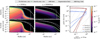Fig. 1 Comparison between the full coagulation model DustPy (upper row, 171 dust fluids) and our new three-parameter power-law prescription TriPoD, which we implemented in the PLUTO code (two dust fluids). We show two snapshots of the one-dimensional disk models in the first two panels in each row. The third panel shows the local dust size distribution of the respective model at 10 au for both snapshots. The light grid in the background represents size distribution power laws with n(a) ∝ a−3.5 and n(a) ∝ a−3.0.

2 Theory

2.1 Dust-gas relative motion

Dust particles moving in the gaseous protoplanetary disk can experience drag forces due to differences between the equilibrium velocities of dust and gas particles. The gas in a PPD is radially stratified, which means the disk has a radial pressure gradient. Consequently, gas moves on a slightly sub-Keplerian orbit, where hydrostatic equilibrium is given by $${\text{Ω}}^2=\frac{1}{R{\rho }_{\text{g}}}\frac{\partial P}{\partial R}+{\text{Ω}}_{\text{K}}^2,$$(1)

where P and ρ_g are the gas pressure and density respectively, R is the cylindrical, stellocentric radius, and ${\text{Ω}}_{\text{K}}^2=G{M}_{*}/R^3$ is the Keplerian angular frequency (see Appendix A for a list of symbols). Conversely, radial pressure forces are negligible for the solid particles, which means their equilibrium orbits would be Keplerian (ignoring the gas drag and additional effects like radiation pressure, etc.). Gas, at velocity ug and dust particles, at velocity ud are aerodynamically coupled via a friction force density $$f_{\text{fric }}={\rho }_{\text{d}}\frac{v_{\text{d}}-v_{\text{g}}}{t_{\text{fric }}},$$(2)

where the strength of the coupling can be characterized by the stopping timescale t_fric. In the Epstein regime (Epstein 1924), the friction time can be written $$t_{\text{fric }}=\sqrt{\frac{\pi }{8}}\frac{{\rho }_{\text{m}}a}{{\rho }_{\text{g}}{c}_{\text{s}}},$$(3)

where ρ_m is the particles’ material density, a denotes the particle radius, and c_s is the sound speed. A useful dimensionless measure of the strength of the coupling between gas and dust particles is the Stokes number St := t_fɪicΩ_K. For St << 1, gas and dust particles are well-coupled and the particles quickly adjust to changes in the gas velocity. For St ≫ 1 however, particles are decoupled from the gas and the friction force is no longer significant for the trajectories of the dust grains.

The stopping time is the timescale on which the particles and the gas approach a steady state. The respective terminal velocities of the grains in force equilibrium were derived by Nakagawa et al. (1986). Ignoring additional velocity components of the gas, for example, due to viscous evolution, the respective relative radial velocity between the grains and the gas then follows as $$v_{\text{d}‐\text{g},R}=\frac{\text{St}(1+\epsilon )}{{\text{St}}^2+{(1+\epsilon )}^2}\frac{1}{{\text{ΩK}}_{}{\rho }_{\text{g}}}\frac{\partial P}{\partial R}$$(4) $$\approx \frac{\text{St}}{{\text{St}}^2+1}\frac{1}{{\text{ΩK}}_{}{\rho }_{\text{g}}}\frac{\partial P}{\partial R}\text{ for \hspace{1em}}\epsilon \ll 1,$$(5)

where ε is the dust-to-gas density ratio. Thus particles drift towards pressure maxima and reach their maximum terminal velocity at a Stokes number of one.

2.2 Dust-dust relative motion

Relative velocities between the gas and dust depend on the aerodynamic properties of the dust. Differently sized grains therefore experience relative velocities due to gas drag. For small grains, Brownian motion is of importance. Additionally, turbulence causes random variations in the gas velocities that act on the dust particles according to their aerodynamic coupling to differently sized eddies in the gas.

Brownian motion. Random molecular motion of particles leads to relative velocities that depend on the respective particles’ masses (Brauer et al. 2008) $$\text{Δ}{v}_{01\text{ Brown }}=\sqrt{\frac{8k_{\text{B}}T\left(m_0+m_1\right)}{\pi m_0{m}_1}},$$(6)

where m₀ and m₁ denote the particles’ masses, T is the gas temperature, and k_B is the Boltzmann constant. This effect is only relevant for the smallest particles on micrometer scales.

Relative drift velocities. For two particles with Stokes numbers St₀ and St₁, the relative drift velocities in the case of low dust-to-gas ratio, are given by Eq. (5) $$\text{Δ}{v}_{01\text{ drift }}=\left|\left(\frac{{\text{St}}_0}{{\text{St}}_0^2+1}-\frac{{\text{St}}_1}{{\text{St}}_1^2+1}\right)\frac{1}{{\text{Ω}}_{\text{K}}{\rho }_{\text{g}}}\frac{\partial P}{\partial R}\right|.$$(7)

Relative settling velocities. Dubrulle et al. (1995) derived the vertical dust distribution in a disk with turbulent diffusion as $${\rho }_{\text{d}}(ɀ)={\rho }_{\text{d},\text{ mid }}\exp \left(-\frac{{ɀ}^2}{2H_{\text{d}}}\right),$$(8)

where H_d is the scale height of the dust, given by $$H_{\text{d}}=\frac{H}{\sqrt{1+\frac{\text{St}}{\delta }}},$$(9)

(see also Fromang & Nelson 2009; Binkert 2023). Here, H refers to the gas scale height, and δ denotes the turbulent diffusivity parameter, which for now is assumed to be equal to the turbulent gas viscosity parameter α. Thus, particles of different sizes are, on average, also found at different heights, and thus have different terminal velocities. The average relative velocities between the two particle populations can then be approximated as $$\text{Δ}{v}_{01\text{ set }}=\left|H_{\text{d}1}{\text{St}}_1-H_{\text{d}0}{\text{St}}_0\right|{\text{Ω}}_{\text{K}}.$$(10)

Relative velocities due to turbulence. Ormel & Cuzzi (2007) derived closed-form expressions for the relative particle velocities in different turbulence regimes, which depend on the Stokes numbers, the turbulent gas velocity, and the local Reynolds number $$\mathrm{Re}=\frac{v_{\text{turb }}}{v_{\text{mol}}}\approx \frac{\alpha c_{\text{s}}H}{c_{\text{s}}{\lambda }_{\text{mfp}}}=\frac{\alpha H{\rho }_{\text{g}}{\sigma }_{{\text{H}}_2}}{\mu m_{\text{p}}},$$(11)

where λ_mfp is the mean free path of the gas molecules, µmp is the mean molecular mass of the gas, and ${\sigma }_{{\text{H}}_2}$ is the collisional cross-section of two gas molecules (here H₂). The respective derivations assume a Kolmogorov turbulent energy cascade (Kolmogorov 1941). We use an implementation of these velocities identical to the one utilized in the full dust coagulation code DustPy.

2.3 Dust coagulation

Dust particles in protoplanetary disks undergo collision since they experience differential velocities due to their interaction with the gas. Surface forces can lead to sticking in such collisions and thus facilitate the growth of dust particles. If collision velocities are too high, they can lead to fragmentation. The Smoluchowski equation (Smoluchowski 1916) describes the evolution of continuous mass (or size) distributions of grains n(m), as a consequence of these processes. In this work, however, we are not numerically solving the coagulation equation as in full- fledged coagulation models like DustPy (Stammler & Birnstiel 2022). Instead, we use the results gained with such elaborate numerical methods to construct a simplified, semi-analytic prescription for dust coagulation. For this, it is instructive to have a look at some main results obtained with full coagulation models and simple analytic derivations. One of these simplifying assumptions is a monodisperse size distribution.

Kornet et al. (2001) have shown that for such a case, the particle growth rate can be written as $$\dot{a}=\frac{{\rho }_{\text{d}}}{{\rho }_{\text{m}}}\text{Δ}v,$$(12)

where Δv denotes the relative velocity between the grains. If the relative velocities are assumed to be caused by gas turbulence in the fully intermediate regime, one finds that the growth of the particles is occurring on a timescale $$t_{\text{grow }}=\frac{1}{\epsilon {\text{Ω}}_{\text{K}}}.$$(13)

However, dust grains can only grow in size as long as their relative velocities due to different aerodynamic properties are not above a critical fragmentation velocity v_frag , for which collisions would lead to the destruction of the particles. Another possible outcome of grain collisions is bouncing, as shown by laboratory experiments (Güttler et al. 2010) and studied in numerical models (Zsom et al. 2010; Dominik & Dullemond 2024). It is possible to derive analytic estimates for the maximum reachable particle size, given a certain fragmentation velocity. Birnstiel et al. (2012) derived the respective maximum particle size in the turbulent fragmentation limit as $$a_{\text{turb-frag }}=\sqrt{\frac{8}{\pi }}\frac{{\rho }_{\text{g}}}{3{\rho }_{\text{m}}}\frac{v_{\text{frag }}^2}{\alpha c_{\text{s}}{\text{Ω}}_{\text{K}}}.$$(14)

Furthermore, dust grains undergo radial drift, which results in relative velocities between grains of different sizes (see Eq. (5)). The resulting collisions can also lead to a drift-fragmentation limit, which is given by $$a_{\text{drift-frag }}=\sqrt{\frac{8}{\pi }}\frac{{\rho }_{\text{g}}}{{\rho }_{\text{m}}}\frac{v_{\text{frag}}}{c_{\text{s}}}\frac{P}{1-\mathcal{N}}{\left|\frac{\partial P}{\partial r}\right|}^{-1},$$(15)

where the constant 𝒩 is approximately 0.5 (Birnstiel et al. 2012). Dust particles can thus not reach sizes larger than $$a_{\text{frag }}=\min \left(a_{\text{drift-frag }},a_{\text{turb-frag }}\right).$$(16)

In these cases, the typically reached size distributions are approximately power laws with characteristic exponents. Birnstiel et al. (2011) used coagulation simulations and analytical calculations to find these fragmentation-limited size distributions. They derived analytic expressions for the resulting power-law exponent of a mass distribution $n(m)\propto m^{-q_{\text{m}}}$ in three different regimes, translating to the size distribution $n(a)\propto a^q=a^{-3q_m+2}$. If coagulation and fragmentation happen simultaneously, the power-law exponent can be written as $$q=2-\frac{3}{2}(v+\xi +1),$$(17)

where ν is a kernel index that depends on how the relative velocities change with particle size. The parameter ξ determines the typical distribution of fragments in a destructive collision. It is usually set to the canonical value of 11/6. Birnstiel et al. (2011) determined that in the first regime of turbulence, as derived by Ormel & Cuzzi (2007), where the relative velocities scale linearly with particle size, v = 1 and thus q = −3.75. The same is true for relative drift velocities, which also linearly depend on the difference in Stokes numbers between the colliding particles (as long as St ≪ 1). This means that typical size distributions in coagulation-fragmentation equilibrium, with collisions driven by differential drift or the first regime of turbulence, can be approximated as power laws n(a) ∝ a^−3.75 , as illustrated in Fig. 2. This case is thus relevant whenever the particle fragmentation velocity is low and only small particles exist, or if the drift velocities dominate over the turbulent velocities, as in the outer regions of protoplanetary disks.

The other prominent case is relevant whenever turbulence is causing relative velocities between particles in the so-called fully intermediate regime. Then, v = ⅚, and one finds that q = −3.5, which is equal to the Mathis et al. (1977) (MRN) distribution. This particular case is relevant in the inner parts of protoplane- tary disks, where the particles grow to the largest sizes and where radial drift is less relevant.

Finally, we have the stages of dust growth in which the fragmentation barrier is not yet reached and the largest particles are undergoing a sweep-up growth. In this case, typical size distributions are steeper and we assume q = -3.0 in this case (Simon et al. 2022; Birnstiel 2023).

Radial drift itself also sets a limit to the maximum particle size, which is reached when the radial drift time scale becomes equal to the local growth time scale $$\begin{array}{l}\frac{a_{\text{drift}}}{\dot{a}}\stackrel{!}{=}\frac{R}{\left|\dot{R}\right|}\hfill \\ a_{\text{drift}}=\sqrt{\frac{8}{\pi }}\frac{{\rho }_{\text{d}}}{{\rho }_{\text{m}}}\frac{v_{\text{K}}}{c_{\text{s}}\gamma },\hfill \end{array}$$(18)

where v_K is the Keplerian velocity and $\gamma =\left|\frac{\text{d\hspace{0.17em}}\log P}{ \text{d\hspace{0.17em}}\log R}\right|$ denotes the radial double-logarithmic pressure gradient. The drift limit is relevant in the outer regions of protoplanetary disks, where drift can become rapid for large particles. In the drift limit, grains do not undergo fragmentation. Therefore, typical size distributions are sweep-up dominated and accordingly steep. We assume q = −3.0, which is typically a good fit to full coagulation simulations.

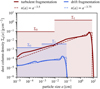Fig. 2 Typical size distributions in regions of a protoplanetary disk model that are either turbulence-dominated (dark red lines) or drift- dominated (blue lines). Both regimes result in distinct power-law exponents of the distribution that we overplot as dashed lines. Assuming a power law as the overall shape of the distribution makes it possible to approximately describe it with only three parameters: The cutoff particle size amax and the two densities Σ0 (contained in the size interval [$a_{\min },\sqrt{a_{\max }{a}_{\min }}$) and Σɪ (contained in the size interval [$\sqrt{a_{\max }{a}_{\min }},a_{\max }$]). This approximation is the basis of our new dust coagulation model.

2.4 The two-pop-py model by (Birnstiel et al. 2012)

With two-pop-py, Birnstiel et al. (2012) introduced a strongly simplified and very fast method to model the effects of dust coagulation in protoplanetary disks. In this method, dust is realized as a single fluid that drifts relative to the gas. The flux calculation, however, considers two dust species. The small population represents the monomers with fixed size a_mon and is assumed to move along with the gas. Larger, grown grains make up the population of size a_gr(t), which is evolving in time, following the monodisperse dust growth rate, which is limited by the above-discussed growth barriers $$a_{\text{gr}}(t)=\min \left[\min \left(a_{\text{drift }},a_{\text{turb-frag }},a_{\text{drift-frag }}\right),a_{\text{mon}}\exp \left(\frac{t-t_0}{t_{\text{grow }}}\right)\right],$$(19)

to simulate the initial phase of coagulation and the growth limits. Both species are associated with a drift velocity according to their Stokes numbers ${\text{St}}_{\text{mon}/\text{gr}}=a_{\text{mon}/\text{gr}}{\rho }_{\text{m}}\pi /2{\text{Σ}}_{\text{g}}$, as $$v_{\text{mon}/\text{gr}}=\frac{v_{\text{gas}}}{1+{\text{St}}_{\text{mon}/\text{gr}}^2}+\frac{{\text{St}}_{\text{mon}/\text{gr}}}{1+{\text{St}}_{\text{mon}/\text{gr}}^2}\frac{1}{{\rho }_{\text{g}}{\text{Ω}}_K}\frac{\partial P}{\partial r},$$(20)

where the first term takes into account gas velocities arising from viscous disk evolution and the second term is the radial drift velocity derived by Nakagawa et al. (1986) in the limit of small dust-to-gas ratios. The total dust flux velocity follows as a mass average of both populations, via $$\overline{v}=\left(1-f_{\text{m}}\right)v_{\text{mon}}+f_{\text{m}}{v}_{\text{gr}}.$$(21)

The ratio f_m is dependent on the limiting factor of grain growth: fragmentation-limited, drift-fragmentation-limited, drift-limited, or neither when the dust is still in the growth phase $$f_{\text{m}}=\{\begin{array}{l}0.97\text{ if }{a}_{\text{drift}}<a_{\text{frag}},a_{\text{drift-frag }}\hfill \\ 0.75\text{ otherwise}.\hfill \end{array}$$(22)

Given the resulting velocity, a flux can be calculated that is used to evolve the dust surface density in time. This method is fast and can be easily implemented in a hydrodynamics code. It has however some serious drawbacks:

• Dust growth is always assumed to be limited by an equilibrium of either fragmentation and coagulation or drift and coagulation. This is mostly true if no substructure is present. In some situations like planetary gaps, however, fluxes and grain sizes are no longer determined by coagulation in the gap but by the supply of small grains that diffuse into the gap and the efficient removal of larger grains. In such cases, grain sizes can be underestimated by two-pop-py, which would assume the drift limit.

• Although the maximum grain size is known, no information on the actual size distribution is provided beyond the knowledge of whether the distribution is drift-limited or fragmentation-limited.

• The differences between the size distribution in the fragmentation limit and the drift-fragmentation limit are not taken into account. The mass fraction fm only considers whether the maximum particle size is drift-limited.

• As growth is always assumed to be driven by collisions in the fully intermediate regime of turbulence, the actual growth timescale can be underestimated (Powell et al. 2019).

• The fragmentation limit is reached instantaneously and not gradually. This is especially problematic if the timescale for dust advection is short.

• The model is only calibrated to reproduce the dust size evolution in protoplanetary disks around 1 M_⊙ stars.

• The model overestimates the concentration of dust in pressure bumps due to the treatment of dust being transported as one fluid. Although the flux is calculated in a mass-averaged way that has been determined experimentally, intermediately sized grains are neglected, which would lead to a wider dust distribution in pressure bumps.

With our new model, TriPoD, we aim to mitigate these problems.

3 The TriPoD model

Our new three-parameter dust evolution model TriPoD makes use of the knowledge gained from full-fledged coagulation models that are discussed in the previous section. In particular, the power-law prescriptions of the dust size distribution are the basis on which we build our method. TriPoD describes the power-law size distribution with only three parameters: the dust column densities of a small population Σ₀ and the large population Σ₁, as well as a maximum particle size a_max at which the distribution is truncated (see Appendix A for a list of symbols used in the context of TriPoD). The populations are separated at the size $a_{\text{int}}=\sqrt{a_{\min }{a}_{\max }}$, which then defines the power-law exponent of a full size distribution via $$q=\frac{\log \left({\text{Σ}}_1/{\text{Σ}}_0\right)}{\log \left(a_{\max }/a_{\text{int}}\right)}-4.$$(23)

Note, that this formula is in general independent of whether we describe a size distribution in the sense of column densities or volume densities. Although we develop the TriPoD method in this paper for use in vertically integrated size distributions, we could also do so for volume densities. In the following, we will thus oftentimes use the dust-to-gas ratio ε, which can be interpreted as either the vertically integrated, or the local version. Assuming the dust size distribution to follow a truncated power law n(a) ∝ a^q, we can write the dust-to-gas ratio size distribution as ε(a) ∝ a^qm ∝ a^qa³. Normalizing this to the total dust-to-gas ratio ε_tot, we get $$\epsilon (a)=\{\begin{array}{ll}\frac{{\epsilon }_{\text{tot}}(q+4)}{a_{\max }^{q+4}-a_{\min }^{q+4}}{a}^{q+3}\hfill & \text{ for }q\ne -4\hfill \\ \frac{{\epsilon }_{\text{tot}}}{\log \left(a_{\max }\right)-\log \left(a_{\min }\right)}\frac{1}{a}\hfill & \text{ for }q=-4,\hfill \end{array}$$(24)

where a_min is the minimum particle size and a_max is the maximum particle size of the truncated distribution. From this, the dust-to-gas ratio within a given size interval [a _I, a _II] with a_min ≤a_I < a_II ≤ a _max, can be calculated as $$\begin{array}{l}{\epsilon }_{a_{\text{I}}}^{a_{\text{II}}}:={\displaystyle {\int }_{a_{\text{I}}}^{a_{\text{II}}}\epsilon \left(a\right)}\text{d}a\\ =\{\begin{array}{ll}{\epsilon }_{\text{tot }}\frac{a_{\text{II}}^{q+4}-a_{\text{I}}^{q+4}}{a_{\max }^{q+4}-a_{\min }^{q+4}}\hfill & \text{ for }q\ne -4\hfill \\ {\epsilon }_{\text{tot }}\frac{\log \left(a_{\text{II}}\right)-\log \left(a_{\text{I}}\right)}{\log \left(a_{\max }\right)-\log \left(a_{\min }\right)}\hfill & \text{ for }q=-4.\hfill \end{array}\end{array}$$(25)

Similarly, the mass-averaged particle size of this distribution is defined as $$\begin{array}{l}{\langle a\rangle }_{a_1}^{a_{11}}:=\frac{{\displaystyle {\int }_{a_{\text{I}}}^{a_{\text{II}}}\epsilon }(a)a \text{d}a}{{\displaystyle {\int }_{a_{\text{I}}}^{a_{\text{I}}}\epsilon }(a)\text{d}a}\\ =\{\begin{array}{ll}\frac{a_{\text{II}}{a}_{\text{I}}}{a_{\text{II}}-a_{\text{I}}}\log \left(\frac{a_{\text{II}}}{a_{\text{I}}}\right)\hfill & \text{ for }q=-5\hfill \\ \frac{q+4}{q+5}\frac{a_{\text{II}}^{q+5}-a_{\text{I}}^{q+5}}{a_{\text{II}}^{q+4}-a_{\text{I}}^{q+4}}\hfill & \text{ for }q\ne -5,-4\hfill \\ \frac{a_{\text{II}}-a_{\text{I}}}{\log \left(a_{\text{II}}\right)-\log \left(a_{\text{I}}\right)}\hfill & \text{ for }q=-4.\hfill \end{array}\end{array}$$(26)

In the TriPoD model, we define two particle populations that together contain the entire dust density of the distribution $$\begin{array}{c}{\epsilon }_0={{{\displaystyle \int }}^{\text{}}}_{a_{\min }}^{a_{\text{int}}}\epsilon (a)\text{d}a\\ {\epsilon }_1={{{\displaystyle \int }}^{\text{}}}_{a_{\text{int}}}^{a_{\max }}\epsilon (a)\text{d}a.\end{array}$$(27)

The mass-averaged particle sizes of both populations are then given by $a_0:={\langle a\rangle }_{a_{\text{min }}}^{a_{\text{int }}}$ and $a_1:={\langle a\rangle }_{a_{\text{int }}}^{a_{\max }}$ (see Eq. (26)). It can be shown that the two populations ε₀ and ε₁ exactly represent the power-law distribution if a_int is defined as the geometric mean of the maximum and minimum size $a_{\text{int}}=\sqrt{a_{\max }{a}_{\min }}$. The power-law exponent q is then given by Eq. (23). Knowing only ε₀ and ε₁ and the maximum size a_max thus allows us to reconstruct the entire size distribution.

On a size grid with N cells a_i, spanning from a_min to a_N ≥ a_max, we can write the mass in a single size bin, and likewise the entire size distribution as $${\epsilon }_i=\{\begin{array}{ll}{\epsilon }_{\text{tot }}\frac{a_{i+\eta /2}^{q+4}-a_{i-1/2}^{q+4}}{a_{\max }^{q+4}-a_{\min }^{q+4}}\theta (a)\hfill & \text{ for }q\ne -4\hfill \\ {\epsilon }_{\text{tot }}\frac{\log \left(a_{i+1/2}\right)-\log \left(a_{i-1/2}\right)}{\log \left(a_{\max }\right)-\log \left(a_{\min }\right)}\theta (a)\hfill & \text{ for }q=-4,\hfill \end{array}$$(28)

where a_i−½ and a_i+½ denote the cell interfaces on the size grid, ${\epsilon }_{\text{tot}}={\displaystyle {\sum }_{i=0}^N{\epsilon }_i}$ is the total dust-to-gas density ratio and θ(a) = Θ(a_i − a_min)Θ(a_i − a_max) represents two Heaviside step functions that cut off the distribution at the minimum and maximum particle sizes. This means we can directly compare our model results with full dust coagulation models like DustPy, which evolve a large grid of sizes instead of just two fluids in our case. We illustrate this in Fig. 2, where we overplot the detailed size distributions, obtained with a full coagulation model, with their respective three-parameter size distribution representation. The respective dust column densities Σ₀ and Σ₁ of the two populations are shown as the horizontal bars spanning the respective size ranges.

In the following, we describe how we evolve the three-parameter size distribution (i.e., ε₀, ε₁ and a_max) in time, using a semi-analytic description of dust coagulation. The prescriptions given in this paper represent the first iteration of our new TriPoD model that is derived and calibrated for vertically integrated disk models. Therefore, all calculations include gas and dust column densities instead of volume densities.

3.1 Particle growth (evolution of a_max)

We model particle growth within the monodisperse approximation (Eq. (12)). The growth limits are realized by comparing a given fragmentation velocity υ_frag with the velocities between large grains ∆υ_max, given by turbulence, differential settling and drift, and Brownian motion. For this, we modify our growth rate by a sigmoid-like function, which leads to growth for ∆υ_max < υ_frag, and decay for ∆υ_max > υ_frag, resulting in $${\dot{a}}_{\max }=\frac{{\text{Σ}}_1\text{Δ}{v}_{\max }}{{\rho }_{\text{m}}\sqrt{2\pi }{H}_1}\left(\frac{1-{\left(\frac{v_{\text{frag }}}{\text{Δ}{v}_{\max }}\right)}^s}{1+{\left(\frac{v_{\text{frag }}}{\text{Δ}{v}_{\max }}\right)}^s}\right),$$(29)

with s being a parameter controlling the steepness of the transition from growth to fragmentation, H₁ being the scale height of large dust grains. The relative grain velocity ∆υ_max is defined between grains of size a_max and f_∆υa_max, where f_∆υ ∊ (0,1) is a model parameter. Determining f_∆υ and s is the main task during the calibration of our model with respect to the full coagulation code DustPy (see Section 4.1 and the red numbers in Table 2).

3.2 Fragmentation and sweep-up (evolution of Σ₀ and Σ₁)

In our model, two effects account for the evolution of the three-parameter size distribution and the interaction between the populations; fragmentation transfers mass from the large population to the small population, while collisions between larger and smaller particles lead to sweep-up, and thus mass transfer from the small bin to the large bin. Erosion of large particles due to collisions with small grains is not accounted for in our model. We describe the sweep-up process via the collision rates between large and small particles $${\dot{\rho }}_{\text{d},0\to 1}=\frac{{\rho }_{\text{g}}^2{\epsilon }_0{\epsilon }_1}{m_0{m}_1}{\sigma }_{01}\text{Δ}{v}_{01}{m}_0,$$(30)

where m₀ and m₁ are the representative particle masses, ∆υ₀₁ is the representative relative velocity between the large and small particles, and σ₀₁ is the representative collision cross section. These quantities are derived from the respective population’s mass-averaged particle sizes (see Eq. (26)).

Fragmentation predominantly occurs in collisions between two large grains. The corresponding transfer rate is thus determined by the collision rates between large grains $${\dot{\rho }}_{\text{d},1\to 0}=\frac{{\rho }_{\text{g}}^2{\epsilon }_1^2}{m_1^2}{\sigma }_{11}\text{Δ}{v}_{11}{m}_1ℱ.$$(31)

Here ℱ represents a function that regulates the relative effectiveness of sweep-up and fragmentation. It is a function of the grain size, the desired power-law exponent of the size distribution, and the relative velocities ∆υ₁₁, defined for collisions between particles of size a₁ and f_∆υa₁. As we cannot model the micro-physics of collisions between grains in our simplified framework for dust evolution, we base the functional form of ℱ on the well-understood results of full coagulation models, which treat the evolution of the size distribution as the result of collisions between grains of all present sizes.

For this first version of our three-parameter model, we are only considering vertically integrated disk models, which means our mass transfer rates are given by $${\dot{\sum }}_{0\to 1}=\frac{{\text{Σ}}_0{\text{Σ}}_1{\sigma }_{01}\text{Δ}{v}_{01}}{m_1\sqrt{2\pi \left(H_0^2+H_1^2\right)}}$$(32) $${\dot{\sum }}_{1\to 0}=\frac{{\text{Σ}}_1^2{\sigma }_{11}\text{Δ}{v}_{11}}{m_1\sqrt{4\pi H_1^2}}\widetilde{ℱ},$$(33)

(see Appendix B). In order to determine the vertically integrated version of ℱ, named $\widetilde{ℱ}$, we consider the steady state between fragmentation and sweep-up. In this equilibrium, a steady size distribution would be reached. Given ${\dot{\text{Σ}}}_{\text{d},0\to 1}={\dot{\text{Σ}}}_{\text{d},1\to 0}$, we arrive at $$\widetilde{ℱ}=\sqrt{\frac{2H_1^2}{H_0^2+H_1^2}}\frac{{\sigma }_{01}}{{\sigma }_{11}}\frac{\text{Δ}{v}_{01}}{\text{Δ}{v}_{11}}{\left(\frac{a_{\max }}{a_{\text{int }}}\right)}^{-(q+4)},$$(34)

where q is the desired power-law exponent of the distribution which will be reached on the dominating collisional timescale.

Mass redistribution due to sweep-up and fragmentation is realized by defining the source terms of both populations in a total-mass-conserving manner as $$\begin{array}{l}{\dot{\text{Σ}}}_0={\dot{\text{Σ}}}_{1\to 0}-{\dot{\text{Σ}}}_{0\to 1}\\ {\dot{\text{Σ}}}_1=-{\dot{\text{Σ}}}_0\end{array}.$$(35)

Determining the size distribution power-law exponent q

We have summed up the typical particle size distribution exponents in Section 2.3, which were determined by Birnstiel et al. (2011) for distributions in coagulation-fragmentation equilibrium. These are given by $$q_{\text{frag }}=\{\begin{array}{ll}{q}_{\text{turb}.1}=-3.75\hfill & \text{ small particle turb}.\text{ regime }\hfill \\ q_{\text{turb}.2}=-3.5\hfill & \text{ fully intermediate turb}.\text{ regime }\hfill \\ q_{\text{drift-frag }}=-3.75\hfill & \text{ drift-dominated regime }\hfill \end{array}$$

q_sweep = −3.0 not in equilibrium (see Birnstiel 2023).

Our task is now to find a way to smoothly switch between these regimes in our three-parameter coagulation model depending on which regime is prevailing under the given conditions.

Firstly, we can determine whether to apply the equilibrium size distributions q_frag or whether the dust has not yet reached coagulation-fragmentation equilibrium and collisions lead predominantly to sticking which results in q_sweep. For this, we define a transition function $$\begin{array}{l}{p}_{\text{frag }}:=\{\begin{array}{l}\to 1\text{ for Δ}{v}_{\max }>v_{\text{frag }}\hfill \\ \to 0\text{ for Δ}{v}_{\max }<v_{\text{frag }}\hfill \end{array}\\ \begin{array}{c}{p}_{\text{sweep }}=1-p_{\text{frag }}\\ \Rightarrow q=q_{\text{frag }}\cdot p_{\text{frag }}+q_{\text{sweep }}\cdot p_{\text{sweep }}\end{array}\end{array}$$(36)

We now have to determine the equilibrium size distribution exponent p_frag. For this, we can again define transition functions. We determine whether the small particle turbulence regime (turb.1) or the fully intermediate regime (turb.2) dominates the relative turbulent velocities $$\begin{array}{l}\begin{array}{c}{p}_{\text{turb}.1}:=\{\begin{array}{c}\to 1\text{ for Δ}{v}_{\text{turb}.1}>\text{Δ}{v}_{\text{turb}.2}\\ \to 0\text{ for Δ}{v}_{\text{turb}.1}<\text{Δ}{v}_{\text{turb}.2}\end{array}\\ p_{\text{turb}.2}=1-p_{\text{turb}.1}\\ \Rightarrow q_{\text{turb-frag }}=q_{\text{turb}.1}\cdot p_{\text{turb}.1}+q_{\text{turb}.2}\cdot p_{\text{turb}.2}.\end{array}\\ \end{array}$$(37)

Lastly, we must determine whether we are in the turbulence-dominated regime or in the drift-dominated regime. Similar to before, we define $$\begin{array}{c}{p}_{\text{drift }}:=\{\begin{array}{c}\to 1\text{ for Δ}{v}_{\text{drift }}>\text{Δ}{v}_{\text{turb }}\\ \to 0\text{ for Δ}{v}_{\text{drift }}<\text{Δ}{v}_{\text{turb }}\end{array}\\ p_{\text{turb }}=1-p_{\text{drift }}\\ \Rightarrow q_{\text{frag }}=q_{\text{drift-frag }}\cdot p_{\text{drift }}+q_{\text{turb-frag }}\cdot p_{\text{turb }},\end{array}$$(38)

where q_turb-frag comes from Eq. (37). With this, we have everything we need to calculate q from Eq. (36) and we can determine the mass exchange rates from Eq. (35). The exact form of the transition functions is not of great importance as long as the transition is sufficiently fast but still smooth enough to not cause issues during numerical integration. The choices that worked best in our subsequent tests are listed in Appendix C.

3.3 Passive dust fluids (in the PLUTO code)

We use the PLUTO¹ code to solve the equations of hydrodynamics in our calibration and test simulations with TriPoD. The Euler equations, solved by PLUTO, read $$\frac{\partial {\rho }_{\text{g}}}{\partial t}+\mathbf{\nabla }\cdot \left({\rho }_{\text{g}}v\right)=0$$(39) $$\frac{\partial {\rho }_{\text{g}}v}{\partial t}+\mathbf{\nabla }\cdot \left({\rho }_{\text{g}}v\otimes v\right)=-\mathbf{\nabla }P-{\rho }_{\text{g}}\mathbf{\nabla }\text{Φ}+\mathbf{\nabla }\cdot \mathbb{T},$$(40)

where υ is the gas velocity vector, Φ is the gravitational potential, and 𝕋 is the viscous stress tensor. The ideal equation of state is used as a closure relation $$P=\frac{k_{\text{B}}T}{\mu m_{\text{p}}}{\rho }_{\text{g}}.$$(41)

The PLUTO code allows for the treatment of passive tracer fluids, which are simply advected with the gas following $$\frac{\partial \left({\rho }_{\text{g}}\epsilon \right)}{\partial t}+\nabla \cdot \left(\epsilon {\rho }_{\text{g}}{v}_{\text{g}}\right)=0.$$(42)

In this work, we consider vertically integrated protoplanetary disks and the advected quantities in our TriPoD model are thus the local dust-to-gas ratios of our two dust populations ε₀ = Σ₀/Σ_g and ε₁ = Σ₁/Σ_g. The maximum particle size is defined as a tracer of the large dust population, meaning our third tracer fluid is a_maxε₁.

The respective tracer fluxes are modified to simulate a dust fluid that is aerodynamically coupled to the gas and thus undergoes radial and azimuthal drift (in the terminal velocity approximation). To achieve this within PLUTO’s tracer prescription, we add a flux component corresponding to the relative velocity between dust and gas $$v_{{\text{Σ}}_{0/1}}=\frac{{\text{St}}_{{\text{Σ}}_{0/1}}}{{\text{St}}_{{\text{Σ}}_{0/1}}^2+1}\frac{1}{{\text{ΩK}}_{}{\rho }_{\text{g}}}\mathbf{\nabla }P,$$(43)

where ${\text{St}}_{{\text{Σ}}_{0/1}}$ is the mass-averaged Stokes number of the respective population. The drift velocities are limited to a fraction of the soundspeed. The third tracer (a_maxε₁) is given the same drift velocity as the large dust population (ε₁). The tracer fluxes are calculated with the upstream dust density and density-weighted maximum particle size based on the drift velocities at the respective cell interface as $$F_{{\text{Σ}}_{0,i+1/2}}^{\text{drift }}={\text{Σ}}_{0,i}\max \left(0,v_{{\text{Σ}}_0,i+1/2}\right)+{\text{Σ}}_{0,i+1}\min \left(v_{{\text{Σ}}_0,i+1/2},0\right)$$(44) $$F_{{\text{Σ}}_1,i+1/2}^{\text{drift }}={\text{Σ}}_{1,i}\max \left(0,v_{{\text{Σ}}_1,i+1/2}\right)+{\text{Σ}}_{1,i+1}\min \left(v_{{\text{Σ}}_1,i+1/2},0\right)$$(45) $$\begin{array}{c}{F}_{a_{\max }{\text{Σ}}_1,i+1/2}^{\text{drif}t}=a_{\max ,i}{\text{Σ}}_{1,i}\max \left(0,v_{{\text{Σ}}_1,i+1/2}\right)\\ +a_{\max ,i+1}{\text{Σ}}_{1,i+1}\min \left(v_{{\text{Σ}}_1,i+1/2},0\right).\end{array}$$(46)

Dust diffusion is implemented in a flux-limited manner, where the transport velocity is limited to the turbulent gas velocity $v_{\max }=\frac{\sqrt{\delta }{c}_{\text{s}}}{1+{\text{St}}^2}$. The diffusion fluxes are given by $$F_{{\text{Σ}}_0,i+1/2}^{\text{diff}}=-{\lambda }_{\lim }\frac{\delta c_{\text{s}}H}{1+{\text{St}}_0^2}{\text{Σ}}_{\text{g},i+1/2}\mathbf{\nabla }{\epsilon }_0$$(47) $$F_{{\text{Σ}}_1,i+1/2}^{\text{diff}}=-{\lambda }_{\lim }\frac{\delta c_{\text{s}}H}{1+{\text{St}}_1^2}{\text{Σ}}_{\text{g},i+1/2}\mathbf{\nabla }{\epsilon }_1$$(48) $$F_{a_{\max }{\text{Σ}}_1,i+1/2}^{\text{diff}}=-{\lambda }_{\lim }\frac{\delta c_{\text{s}}H}{1+{\text{St}}_1^2}{\text{Σ}}_{\text{g},i+1/2}\mathbf{\nabla }\left(a_{\max }{\epsilon }_1\right),$$(49)

where λ_lim is the respective flux limiter function (see Appendix D). All quantities are interpolated to the cell interface. The drift and diffusion fluxes are added to the advective flux of the dust fluids stemming from the gas motion. We have used this approach in Pfeil et al. (2023), where we also presented some simple test cases of the method. Note that this approach makes use of the terminal velocity approximation and is thus strictly speaking only valid for St ≪ 1. The TriPoD model itself, being a local model, is not bound to this form of dust advection scheme and could be implemented in any multi-fluid-capable hydrodynamics code.

3.4 Complete right-hand side of the conservation equations (in the PLUTO code)

All modifications made for our three-parameter dust evolution model can be applied within the framework of PLUTO and without changing the underlying reconstruct-solve-average scheme of the code.

Source terms are added to the right-hand side of the conservative hydrodynamics equations describing the evolution of the three-parameter dust size distribution in the framework of PLUTO. For each dimension and evolving variable, we have the right-hand side of the conservation equation $${ℛ}_i=-\frac{\text{Δ}t}{\text{Δ}{\mathcal{V}}_i}\left[{(\mathcal{A}F)}_{i+1/2}-{(\mathcal{A}F)}_{i-1/2}\right]+\text{Δ}t{\mathcal{S}}_i,$$(50)

where ∆t is the timestep, ∆𝒱, is the cell volume, 𝒜 the respective cell surface, F is the flux through the interfaces, determined from advection with the gas plus relative terminal velocity and diffusion fluxes, and 𝒮_i is the source term, given by fragmentation, sweep-up, and growth.

For the two dust fluids, the fluxes are calculated via Eqs. (44)–(49), and the source term of the respective dust fluid is calculated from Eq. (35) $$F_{{\text{Σ}}_{0/1},i\pm 1/2}=F_{{\text{Σ}}_{0/1},i\pm 1/2}^{\text{diff}}+F_{{\text{Σ}}_{0/1,i\pm 1/2}}^{\text{drift}}+F_{{\text{Σ}}_{0/1,i\pm 1/2}}^{\text{adv}}$$(51) $${\mathcal{S}}_{{\text{Σ}}_{0/1},i}={\dot{\text{Σ}}}_{0/1,i},$$(52)

where $F_{{\text{Σ}}_{\text{0/1}}\text{,}i\text{±1/2}}^{\text{adv}}$ is the flux component that is calculated by PLUTO for the passive advection of the tracers. The maximum particle size is advected together with a large population as a tracer. The fluxes and growth rate are $$F_{a_{\max }{\text{Σ}}_1,i\pm 1/2}=F_{a_{\max }{\text{Σ}}_1,i\pm 1/2}^{\text{diff}}+F_{a_{\max }{\text{Σ}}_1,i\pm 1/2}^{\text{drift}}+F_{a_{\max }{\text{Σ}}_1,i\pm 1/2}^{\text{adv}}$$(53) $${\mathcal{S}}_{a_{\max }{\text{Σ}}_1,i}=a_{\max ,i}{\text{Σ}}_{1,i}+{\text{Σ}}_{1,i}{a}_{\max ,i}.$$(54)

Here, $F_{a_{\max }{\text{Σ}}_1,i\pm 1/2}^{\text{adv}}$ is the flux component that is calculated by PLUTO for the passive advection of the tracer and ȧ_max is the particle growth rate, given by Eq. (29). The evolution equations are evolved in time with PLUTO’s standard third-order Runge-Kutta routine. The timestep is limited by the CFL condition, which we don’t have to adjust since the dust drift velocities are limited to a fraction of the speed of sound and the typical growth timescale is much longer than an orbital timescale.

4 Calibration

Our model has several free parameters, which have to be calibrated in comparison to full dust coagulation simulations. For the growth rate of the dust (Eq. (29)), the main parameters are s (determining the steepness of the transition from growth to fragmentation), and the parameter f_∆v, which determines the relative velocities ∆υ₁₁ and ∆υ_max through the size ratio between the grains.

We ran a series of one-dimensional simulations for calibration of the model against the full-coagulation code DustPy. We set up a 1D disk model similar to the standard DustPy model. We excluded viscous evolution since we are only interested in comparing the dust evolution in both models for the time being. The radial disk structure follows $$\begin{array}{c}{\text{Σg}}_{}(R)=\left(2+{\beta }_{\text{Σ}}\right)\frac{M_{\text{disk }}}{2\pi R_{\text{c}}^2}{\left(\frac{R}{R_{\text{c}}}\right)}^{{\beta }_{\text{Σ}}}\exp \left[-{\left(\frac{R}{R_{\text{c}}}\right)}^{2+{\beta }_{\text{Σ}}}\right]\\ :={\text{Σ}}_{\text{g},0}{\left(\frac{R}{R_0}\right)}^{{\beta }_{\text{Σ}}}\exp \left[-{\left(\frac{R}{R_{\text{c}}}\right)}^{2+{\beta }_{\text{Σ}}}\right],\end{array}$$(55)

where we employed the code units ∑_g,0 = 733.28 g cm⁻² (derived from a DustPy setup with M_disk = 0.05M_⊙), β_∑ = −0.85, β_T = −0.5, and R₀ = 1 au. In PLUTO, the radial temperature structure is expressed in terms of the speed of sound, which is given by $$\begin{array}{c}{c}_{\text{s}}^2=T_0\frac{k_{\text{B}}}{\mu m_{\text{p}}}={\left(\frac{0.05L_{\ast }}{4\pi R^2{\sigma }_{\text{SB}}}\right)}^{\frac{1}{4}}\frac{k_{\text{B}}}{\mu m_{\text{p}}}\\ :=v_0^2{\left(\frac{H_0}{R_0}\right)}^2{\left(\frac{R}{R_0}\right)}^{{\beta }_T},\end{array}$$(56)

with $v_0=\sqrt{G{M}_{\ast }/R_0}$. In our simulations, this was parameterized by the disk aspect ratio $\raisebox{1ex}{$H_0$}\!\left/ \!\raisebox{-1ex}{$R_0$}\right.$ at reference radius R₀.

The simulations were initialized with a total dust-to-gas ratio of 1%, and an initial maximum particle size of 1 µm. Particles larger than the initial drift limit were excluded from the initial dust profile to avoid an inwards drifting wave of large dust at the beginning of the simulation. The initial dust size distribution in both DustPy and TriPoD follows a power law with q = −3.5. The stellar and disk structure parameters are shown in Table 1 and the parameters for the different calibration runs are shown in Table 2.

4.1 Calibrating the growth rate

Determining the appropriate relative grain velocities to reproduce the full coagulation model with our simplified prescription is the topic of this section.

The particle growth rate in our model can be adjusted by varying the relative velocity ∆υ_max in Eq. (29). This is controlled over the parameter f_∆υ ∊ (0, 1), which sets the size ratio between the colliding particles a_max and f_∆υa_max, (∆υ_max) as well as a₁ and f_∆υa₁, (∆υ₁₁). We have thus determined which particle size ratio best reproduces the relative velocity that determines the overall growth rate. Furthermore, the parameter s in Eq. (29) can be used to adjust the growth rate around the transition from growth to fragmentation, where a small s corresponds to a reduced growth rate close to the fragmentation limit, and a large s corresponds to a steep transition from particle growth to fragmentation-coagulation equilibrium.

To characterize the effects in comparison with the full coagulation model DustPy, we measured the rate of change of the mass-averaged particle size in TriPoD and DustPy and determined the respective deviations for the given parameters. We used the mass-averaged size and not the maximum particle size because it is also a measure of the shape of the size distribution itself and not just the upper cutoff. To calibrate the growth rate we ran DustPy and TriPoD models without transport (all fluxes are zero). We were, however, still considering the relative drift and sedimentation velocities in the calculation of ∆υ₀₁, ∆υ₁₁ and ∆υ_max. We set up the disk models for a solar-mass pre-main-sequence star with a 0.05 M_⊙ gas disk and a dust-to-gas ratio of 1% (see Tables 1 and 3 for details).

First, we ran a parameter study for the factor f_∆υ. This parameter can be physically interpreted as the particle size ratio in the collisions that dominate the growth process. Since we know that growth is dominated by particle collisions where the size difference between projectile and target is not too large, we chose values between 0.2 and 0.6. As can be seen in Fig. 3, a factor of f_∆υ = 0.4 leads to the overall best agreement between the particle growth rate in TriPoD and DustPy.

The second parameter setting the growth rate is s, which determines the steepness of the transition from growth to fragmentation in Eq. (29). We know that this transition is usually not leading to an instantaneous cutoff of the growth rate. In reality, the particles have collision velocities following a Maxwell-Boltzmann distribution (Stammler & Birnstiel 2022). Very large values of s would thus lead to a time evolution that does not agree well with DustPy. We ran models with values from 2 to 6, which we compared in Fig. 4. As can be seen, a value of s = 3 leads to the best fit between the growth rates close to the fragmentation limit.

4.2 Calibrating the dust transport

Dust transport is realized by modifying the dust tracer flux (see Section 3.3). For this, the mass-averaged particle size of each dust population is calculated to determine the upstream flux through the respective cell interface. This means that the steepness of the size distribution, which determines the amount of mass in each bin, also partially determines the radial mass flux. As discussed in the introduction, the power law’s shape in fragmentation-coagulation equilibrium is well known. In the drift limit, however, it can not be easily deduced from analytical arguments. Numerical dust coagulation simulations with DustPy show that the power law is generally more top-heavy in the drift limit/sweep-up phase and probably best approximated by a value between −2.5 and −3. We have therefore conducted TriPoD simulations covering this parameter range to determine what value best reproduces the late-stage mass evolution of the disk. The mass evolution is generally well reproduced for q_sweep = −3.0, which is why this value is used for all following simulations.

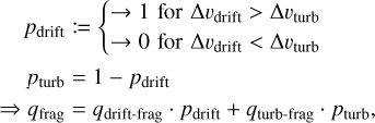
In comparison with a more realistic size distribution, the power-law prescription lacks the gradual decrease in mass, shortly before the maximum particle size (visible in the right panels of Fig. 1). This means that, even if our power-law size distribution reproduces the real size distribution very well, the mass-averaged sizes of both models will not be identical. For this reason, our dust fluxes will also be slightly different from the total flux in DustPy. This is generally not a significant effect. We nonetheless accounted for it by using a calibration factor f_drift that is multiplied to the calculated mass-averaged particle sizes before the calculation of the dust flux, similar to the fudge factor in the two–pop–py model (Birnstiel et al. 2012). For this, we ran models for different values of this calibration factor, including dust transport. We neglected any gas transport in these simulations and focused on the dust fluxes, where we conducted one set of simulations with a dust diffusivity of δ = 10⁻³ and one with δ = 0 (no diffusion). Except for the inclusion of dust transport, the simulations are identical to the setups used in the growth rate calibration. We applied the best-fitting parameters from the growth rate calibration. We use 150 log-spaced radial grid cells to resolve our simulation domain, which was defined between 2 and 250 au. This is the same resolution as used in the DustPy runs. For comparison, we present a time series of the dust column densities in these simulations runs for f_drift =0.6, 0.7, 0.8, 0.9 and 1.0 in the upper row of Fig. 5 (Fig. E.1 depicts the case without diffusion). The lower two panels depict the dust mass evolution (lower left) and the respective deviations from the full coagulation model DustPy (lower right). As can be seen, the choice of f_drift determines the mass flux throughout the disk’s dust evolution. Smaller values of f_drift correspond to slower dust velocities and lower fluxes. All values result in deviations of ≲40% from the full coagulation model at all times. The value of f_drift = 0.8, however, shows the smallest mass error. For this value, the disk’s dust mass only deviates by 10% from DustPy during most of the mass evolution. The absolute error only increases to ≲30 after 90% of the mass has already drifted out of the simulation domain. The overall trend in the mass evolution with f_drift seems to be independent of the diffusion parameter, as can be seen by comparison of Figs. 5 and E.1. We therefore chose a value of f_drift = 0.8 for all following simulations.

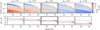Fig. 3 Parameter study for the factor f∆υ, which is the most important parameter for the growth rate calibration of our model. For this, we calculated the deviation between the mass-averaged particle size’s growth rate in DustPy and TriPoD. In the top row, we show models for different global values of f∆υ. It can be seen that f∆υ = 0.4 seems to fit the dust growth rate best.

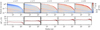Fig. 4 Parameter study for the factor s, which determines the steepness of the transition from sweep-up growth to coagulation-fragmentation equilibrium in Eq. (29). Heat maps show the deviation of the growth rate in TriPoD from the growth rate in DustPy. The lower row shows the average over the size dimension. The influence of a variation in s can be seen around the fragmentation limit, where a larger s corresponds to a steeper transition (fast growth close to the fragmentation limit), while a small s corresponds to a slower transition where growth rates decrease earlier and more slowly. The case of s = 3 has the overall best fit with the DustPy model.

4.3 Treatment of planetary gaps

Since the particle size in TriPoD can only change due to coagulation/fragmentation, we have to introduce an additional source term that takes into account the particle size reduction due to the depletion of large particles via transport. The classic example of such a case is a gap carved by a planet. In this case, dust diffusion into the gap from the outer disk, removal of large grains within the gap, and coagulation determine what particle sizes are present. Due to the pressure maximum at the gap’s outer edge, larger grains can no longer drift into the co-orbital region of a planet. However, smaller particles are still diffused through the pressure maximum by turbulence and thus slightly increase the solid content of the mostly depleted gap. As the largest particles are removed from the gap, we reduce the maximum particle size on the respective dust depletion timescale in TriPoD. For this, we set a lower limit for the fraction of large particles at which we begin the size reduction process. We define a hypothetical source term for ε₁, which would set a lower limit to ε₁ in terms of a critical fraction of the total dust density $\frac{\text{d}{\epsilon }_1}{\text{d}t}=\frac{f_{\text{crit}}\left({\epsilon }_0+{\epsilon }_1\right)-{\epsilon }_1}{\text{Δ}t}$ where ∆t is the current simulation timestep. Since our goal is to reduce the maximum particle size on the depletion timescale, we set ${\tau }_{\text{depletion}}={\epsilon }_1/\frac{\text{d}{\epsilon }_1}{\text{d}t}$ and define the respective size reduction rate $$\frac{\text{d}{a}_{\max }}{\text{d}t}=\frac{a_{\max }}{{\tau }_{\text{depletion }}}\left(1-\frac{a_{\max }}{a_{\text{lim}}}\right),$$(57)

where a_lim = 1 µm is a minimum size that we define to limit the shrinking to a reasonable value. To retain a meaningful power-law exponent for the size distribution during the shrinking process, we set the mass change rate of the large population to $$\frac{\text{d}{\epsilon }_1}{ \text{d}t}=\frac{\partial {\epsilon }_1}{\partial a_{\max }}\frac{\text{d}{a}_{\max }}{\text{d}t}.$$(58)

Here, ${\partial }_{\epsilon }{}_{{}_1}/\partial a_{\max }$ follows analytically from Eq. (25). Equations (57) and (58) are added as source terms to the respective right-hand side of the conservation equations if the condition for size reduction is fulfilled (ε₁ < f_critε_tot). In that way we achieve the following:

• Whenever transport is largely dominating over coagulation, thus removing the large particles, we reduce the maximum particle size on the depletion timescale of the large grain population.

• We thus set a lower limit for the power-law exponent and therefore retain a physically meaningful size distribution, even in planetary gaps.

Determining the critical value of ε₁ at which we begin the size reduction process is an experimental task. The size distribution within a planetary gap is typically not top-heavy due to the efficient removal of the largest grains (e.g., Drazkowska et al. 2019). The large mass bin should thus contain ≲50% of the total dust density in the gap.

We set up a one-dimensional simulation with a gap corresponding to a Jupiter-mass planet, following the description of Duffell (2020) in TriPoD and DustPy. The gap is not evolving in time, but pre-defined in the disk’s gas structure and the initial dust density structure. We ran simulations for several values of the critical mass fraction f_crit to determine which values give us the best fit between TriPoD and DustPy in a planetary gap. For the limiting particle size, we set either 1 µm or 10 µm. The resulting dust column density profiles are shown in Fig. 6. As can be seen, we reached a reasonably good fit for a value of f_crit = 0.425 and a limiting particle size of a_lim = 1 µm. We have therefore chosen these values for all following simulations.

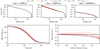Fig. 5 Comparison between DustPy and our model in a setup with dust diffusion (δ = 10−3) and with different drift calibration factors fdrift. Solid lines show the results of our TriPoD calibration runs and dashed lines show the respective DustPy simulation, to which we calibrate our model. The upper row shows a timeseries of the dust column density evolution in three snapshots. In the lower row, we show the mass evolution and the errors with respect to the full coagulation model DustPy. For a factor of fdrift = 0.8, the mass evolution of the full coagulation model is well reproduced by our three-parameter model.

5 Test simulations

Here, we present a series of test cases of our TriPoD model for comparison with DustPy. Our fiducial model is depicted in Fig. 1. We set up a smooth protoplanetary disk around a solar-mass star for this. The disk structure is identical to the simulations in the calibration runs. The first two panels in each row show the snapshots of the dust size distributions in DustPy (top row) and TriPoD after 20500 yr and 3 × 10⁶ yr of evolution. For this run, gas evolution has been turned off to get a more direct comparison between the dust evolution and transport models. The shape of the size distribution is well reproduced in the drift-limited and fragmentation-limited cases.

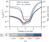Fig. 6 Test for the size reduction in planetary gaps. The dashed lines correspond to the maximum grain size of the respective model (see color bars for the model parameters), while the solid lines show the dust column density for each model. Thick black lines correspond to the respective DustPy simulation that we want to reproduce. The particle size is reduced on the dust depletion timescale when the large dust population makes up less than the critical fraction ƒcrit of the total dust density. We run these simulations to determine which value leads to the best agreement with the DustPy simulation.

5.1 Different stellar masses

We tested the accuracy of our model in simulations of systems with different stellar masses and disk masses. For this, we took the stellar properties of stars with M_* = 0.1, 0.3, 0.5, 0.7 and 0.9 M_⊙ from the pre-main sequence evolution tracks of Baraffe et al. (2015) at ~ 10⁵ yr of evolution (their first recorded snapshot). We kept the overall disk structure constant for all setups with the values from Table and set the disk mass to 0.05 M_*. We ran the simulations for all stellar masses once with dust diffusion and a diffusion parameter of δ = 10⁻³ and once without dust diffusion. Gas evolution was turned off in these simulations, as we were only interested in the accuracy of our dust evolution model. We present three of the simulations with diffusion in Fig. 7, where the first two panels in each row show snapshots of the simulations. The respective DustPy model is shown on top and the TriPoD results below. We found that the overall size distribution evolution is well reproduced for most of the simulation domain and runtime. Our model is also able to capture the shape of the size distributions, as can be seen in the right panels. In the early stages of dust evolution (left panel of each row in Fig. 7), the dust size distribution is in coagulation-fragmentation equilibrium, which results in a typical power-law shape of the distribution with exponent p = −3.5. In the case of the 0.1 M_⊙ star system, the dust is still in its initial growth phase at the time of the earlier snapshot. Therefore, the distribution has not yet fully reached the equilibrium state and is still more top-heavy – which is typical for the growth phase in which smaller particles are swept up by bigger particles. In this phase, the distribution is not so well reproduced by a power law. Our three-parameter model nonetheless captures the steeper slope well around the size distribution peak, which contains most of the mass.

We present a more detailed look at the column density and mass evolution in Fig. 8 (simulations without diffusion can be found in Fig. E.2). The relative mass error with respect to the full coagulation model is always ≲20% until ~90% of the mass has been accreted. The small errors at the beginning of the simulations are seen to add up in the late stages of disk evolution, where the absolute relative mass error in simulations is <35% at the end of the simulation when more than 99% of the mass has drifted out of the simulation domain after 3 × 10⁶ yr.

For stellar masses above 0.3 M_⊙, the errors are even smaller. Here, we determine a deviation of less than 10% until ~90% of the dust mass has drifted out of the simulation domain. Afterward, in the final stages of dust mass evolution, absolute errors increase again and are generally <30%. Only for the system with the least massive star, we measured a maximum deviation of ~35% at the very end of the dust mass evolution. One reason for this could be the smaller disk size, which means the dust growth front reaches the outer edge of the disk earlier. This area of strong radial dust-to-gas ratio gradients seems to be the origin of most of the deviations, as can be seen in the upper right panel of Fig. 8. Overall, the mass evolution in disks around stars of various masses is very well reproduced.

5.2 Varying fragmentation velocity

To assess the accuracy of our model for different fragmentation velocities we chose a simple setup with a temperature-dependent fragmentation velocity. Following² $$v_{\text{frag }}=\{\begin{array}{ll}100 \text{cm} {\text{s}}^{-1}\hfill & \text{ for }T>150 \text{K (ices evaporated) }\hfill \\ 1000 \text{cm} {\text{s}}^{-1}\hfill & \text{ for }150 \text{K}>T>80 \text{K}({\text{H}}_2\text{O}\text{ ice) }\hfill \\ 700 \text{cm} {\text{s}}^{-1}\hfill & \text{ for }80 \text{K}>T>44 \text{K}\left({\text{NH}}_3\text{ ice }\right)\hfill \\ 100 \text{cm} {\text{s}}^{-1}\hfill & \text{ for }44 \text{K}>T\left({\text{CO}}_2\text{ ice }\right),\hfill \end{array}$$(59)

we assumed particles covered in water ice to be the stickiest, followed by NH₃ ice and bare silicates or CO₂ ice. We used this highly simplified model only to illustrate that TriPoD accurately reproduces the DustPy results for setups with different fragmentation velocities. We display the resulting dust size distributions for two snapshots of the simulations in Fig. 9. In the disk regions within ~2au, temperatures exceed 150 K and the fragmentation velocity is accordingly low since all ices are assumed to be evaporated. Thus particles only grow up to millimeter sizes. In the regions beyond the water snow line, we find the two regions with larger fragmentation velocities; first the region with water ice, then, outside of ~8 au the region with ammonia ice which we assigned a slightly lower fragmentation velocity. The outer regions of the disk beyond the CO₂ snow line have again been given the lowest fragmentation velocity and have thus also lower maximum particle sizes. As can be seen in Fig. 9, the overall evolution of the disk and the local dust size distributions in the distinct regions of our DustPy and TriPoD models show excellent agreements in dust column densities and maximum particle sizes.

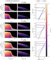Fig. 7 Comparison of the dust size distributions in three simulations with different stellar masses and different disk masses. The first row in each group depicts a DustPy simulation (full treatment of coagulation). The lower rows show the respective TriPoD simulations with the PLUTO code. Panels on the right depict the local dust size distributions at 10 au at both snapshots. The gray lines in the right panel follow power laws with q = −3.5 and q = −3.0.

5.3 Planetary gap

As a next test case, we conducted a simulation with a planet-induced gap. For the gap in our one-dimensional DustPy and TriPoD simulations we used the same gap profile as in Section 4.3. Instead of letting the disk viscously evolve, we again turned off gas evolution for these simulations and imposed the gap profile immediately on the disk’s column density structure. We compare the resulting size distributions in Fig. 10 with a similar DustPy model in the top row. As can be seen, dust particles collect in the pressure maximum outside of the planetary gap. The gap itself becomes depleted of dust, as the particles drift out and cannot be replenished due to the effect of the pressure bump. As a result, the maximum particle size in the full coagulation model is reduced within the gap. As large grains are removed, the maximum particle size is also reduced in TriPoD, and thus a reasonable size distribution is retained. In that way, a good fit with the particle size in the gap of the full coagulation model is achieved. The size distribution in the full coagulation model is no longer top-heavy inside the gap but declines toward smaller sizes. The same is achieved in TriPoD with our size reduction method, as seen in the right panels of Fig. 10. Particles collecting in the pressure bump outside of the gap are fragmentation-limited and can thus grow to larger sizes than in the outer regions, which are drift-limited. Most mass from the outer disk collects around the pressure maximum and does not reach the inner disk.

The size distribution in the regions inside of the gap becomes drift-limited and dust densities decrease significantly due to the decreased inflow from the outer regions. Only diffusion of small particles through the gap maintains some particle flow in the inner disk. For comparison, we also show the dust column densities and maximum particle sizes calculated with the old two-pop-py method in Fig. 10. As can be seen, the new method agrees much better with DustPy. In the two-pop-py simulation, we find a much narrower peak in the dust densities around the pressure maximum due to the lack of a small particle population. Grain sizes are also underestimated in the gap, as two-pop-py sets the maximum particle size to the drift limit. This assumes an equilibrium between transport and coagulation which is not given in the gap, where the present particles are diffusing in from the outer edge and large particles are quickly removed by drift.

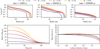Fig. 8 Comparison between DustPy and our model in setups with different stellar masses. Solid lines show the results of our TriPoD simulations and dashed lines show the respective DustPy simulations. The upper row shows a time series of the dust column density evolution in three snapshots. In the lower row, we show the mass evolution and the errors with respect to the full coagulation model DustPy.

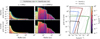Fig. 9 Comparison between a DustPy simulation and a PLUTO simulation with our TriPoD dust coagulation model of a protoplanetary disk with radially varying fragmentation velocity (see Eq. (59)). The left and center columns depict the global dust distribution at two different snapshots of the simulations, with the DustPy simulation in the top row and the TriPoD simulation at the bottom. The right plot shows the local dust size distributions in the second snapshot at the locations of the vertical lines of the same color in the central panel. The gray lines in the right panel follow power laws with q = −3.5 and q = −3.0.

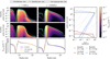Fig. 10 Comparison between a DustPy simulation and a PLUTO simulation with our TriPoD dust coagulation model in a protoplanetary disk with a pre-defined gap. We also show the particle sizes and dust column density profiles calculated with the old two-pop-py model as dotted lines. The plot on the right-hand side depicts the local dust size distributions at 5 au (within the gap) and at 8.5 au (at the pressure maximum), for two different snapshots. The gray lines in the right panel follow power laws with q = −3.5 and q = −3.0.

5.4 Two-dimensional planet-disk simulation

As a last test case, we ran a two-dimensional simulation of a protoplanetary disk with a Jupiter-mass planet. We set up a simulation in polar coordinates. The domain is spanning 4–34 au radially and full 2π azimuthally at a resolution of 1024 cells in the radial and azimuthal direction. The planet is represented by an additional gravitational potential following $${\text{Φ}}_{\text{p}}=-\frac{G{M}_{\text{p}}}{\sqrt{d^2+r_{\text{sm}}^2}},$$(60)

where M_p is the planets mass, d is the distance to the planet, and r_sm = 0.7 H is the gravitational smoothing length. The full gravitational potential in our simulation domain is then given as $${\text{Φ}}_{\text{tot}}={\text{Φ}}_{*}+{\text{Φ}}_{\text{p}},$$(61)

where Φ_* is the gravitational potential of a Solar-mass star. The disk was set up as a radial power law in column density and temperature with an isothermal equation of state. Details on the disk structure and simulation setup can be found in Table 4. We employed a viscosity v = αc_s H, with α = 10⁻³. The hydro-dynamic equations were solved with the HLL Riemann solver, using the third-order accurate Runge-Kutta scheme for the time integration and piece-wise-polynomial spatial reconstruction scheme to the fifth-order.

For the gas velocities, we used a zero-gradient boundary condition at the inner boundary, where we kept the gas density and the azimuthal velocity fixed to the initial values in the ghost cells. Similar boundary conditions were applied at the outer domain edge, with the difference that we allowed for outgoing velocities but not for inflow. The dust densities at the outer boundary were also kept at the initial value for 1000 orbital time scales after which we began to decrease them exponentially on a timescale of 1000 orbits in order to simulate a reduced dust inflow.

We compare the results to a simulation with the two-pop-py model, which only has one dust fluid. The comparison is presented in Fig. 11, where the top row shows the TriPoD simulation, and the middle row shows two-pop-py after 2000 planetary orbits of evolution. In the lower panels, we present the respective quantities’ azimuthal averages, for which we have masked out the region around the planet that has been marked with a white circle.

The different grain sizes and the redistribution of mass because of fragmentation and coagulation between the two populations lead to different dust density distributions in the simulation with TriPoD compared to the simulation with two-pop-py. The grains in the two-pop-py simulation collect in two narrowly peaked overdensities at the pressure maximum outside of the planetary gap and a weak second pressure perturbation. The gap is more depleted than in the simulation with the TriPoD model. Furthermore, dust densities in two-pop-py are strongly enhanced in the weak second pressure perturbation that has almost no visible effect in the simulation with TriPoD. The reason for this is the absence of a smaller, separately advected grain population in two-pop-py for which the effect of trapping would be much weaker. This is accounted for in the TriPoD simulation, where the smaller dust population broadens the dust peaks significantly due to the weaker trapping of small grains. This also has the effect that more dust can diffuse through the gap, which means that the densities inside and in the gap itself are slightly higher in TriPoD than in two-pop-py.

Inside the gap, TriPoD limits the size distribution exponent to a minimum value of q ≈ 4 due to the applied size reduction rates which means the distribution is no longer fragmentation-limited but dominated by transport effects. The particles remaining in the gap are accordingly small and the size distributions are no longer top-heavy, as seen in the work by Drazkowska et al. (2019). The two-pop-py model instead assumes the drift limit in the gap and inside of it. The size distribution, assumed by two-pop-py is thus vastly different from the almost flat or declining distribution seen in TriPoD and in full coagulation models. Similar to the results of Drazkowska et al. (2019), we find that the two-pop-py method still approximates the dust column densities inside of the gap fairly well. The Dust grain sizes are, however, underestimated inside and around the gap and the density profile at the pressure trap is not well reproduced by two-pop-py.

Our results are thus qualitatively similar to the conclusions by Drążkowska et al. (2019). Coagulation makes it possible for small grains to pass through the gap via diffusion and coagulate again inside of the planet’s orbit. The dust accumulates in the pressure bump, but the peak in the dust density is broader than in a simulation without coagulation, due to the presence of small grains, which are constantly produced in our simulation as a result of fragmentation.

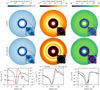Fig. 11 Comparison between two-dimensional PLUTO simulations with the TriPoD coagulation model and with the two-pop-py model. Both simulations have the exact same gas density structure and are only distinguished by the applied dust coagulation model. The lower panels show the azimuthally averaged quantities. For the azimuthal averages, we have masked the region around the planet that has been marked with the white circle. The red line in the left panel shows the radial pressure gradient parameter $\eta =\frac{1}{2}{\left(\frac{H}{R}\right)}^2\frac{\partial \text{\hspace{0.17em}log\hspace{0.17em}}P}{\partial \text{\hspace{0.17em}log\hspace{0.17em}}R}$. It can be seen that in our simulation a weak second pressure maximum appears at ~20 au, which leads to strong trapping in the two-pop-py model (Birnstiel et al. 2012). This effect is much less pronounced if a polydisperse size distribution is considered as done in our TriPoD simulation, where the small dust population is less efficiently trapped.

6 Discussion

In its current form in the PLUTO code, our model operates in the terminal velocity approximation. The dust fluids are implemented as passive tracers with modified fluxes. Thus, feedback from the dust on the gas is not included in our two-dimensional test simulation. However, as shown by Drążkowska et al. (2019), the dust feedback in their two-dimensional planet-disk simulation only had a minor effect on the simulation outcome. Effects like the streaming instability (Youdin & Goodman 2005), cannot be simulated with our current version of TriPoD due to this limitation of our very simple dust fluid implementation. Unfortunately, PLUTO does currently not have a multi-fluid feature. A future iteration of the model could be combined with a code that supports dust fluids that are treated more self-consistently, like FARGO3D (Benítez-Llambay & Masset 2016; Benítez-Llambay et al. 2019) or Athena++ (Stone et al. 2020; Huang & Bai 2022). The terminal velocity approach also means that effects occurring on timescales shorter than the friction timescale of the particles cannot be modeled in the current form of TriPoD. Possible cases could be the effects of shock waves, or spiral density waves.

Another shortcoming arises from the way we calculate the dust fluxes. As the maximum particle size changes throughout a simulation domain, neighboring cells usually do not have the same particle sizes. Therefore, the bin interfaces separating σ₀ and σ₁ are also different between neighboring cells. Our advection scheme does not take this into account in its current form, where transport is only occurring between the same size bin and not across bins. Due to the smooth variation of a_max throughout simulations of protoplanetary disks, neighboring cells will typically still have very similar maximum particle sizes. The effect of this inaccuracy in the advection scheme is therefore likely small. However, one could construct extreme cases in which the error would be large, for example, if two neighboring cells had vastly different maximum particle sizes. We will have to address this issue in a future version of the model.

Details of the grain size distribution that are modeled in full-fledged coagulation models like DustPy cannot be reproduced in our simplified prescription. To still achieve a good fit with such models, our model has several calibration factors that have been adjusted to reach a good fit with DustPy. However, this treatment of dust coagulation cannot reproduce the finer details of the coagulation process.

Our model omits the effects of bouncing (see Dominik & Dullemond 2024). This effect can lead to a steep, top-heavy size distribution and smaller maximum particle sizes. Bouncing could be implemented in a future version of TriPoD.

TriPoD, as well as DustPy are designed to simulate the dust evolution in vertically integrated models of protoplanetary disks, assuming settling-mixing equilibrium at all times. Effects like sedimentation-driven coagulation (Zsom et al. 2011; Krijt & Ciesla 2016) can thus not be modeled by DustPy or TriPoD in its current form. This is however not a fundamental limitation of TriPoD, which could be adapted to work in three-dimensional setups in a future version.

7 Summary and conclusion

We present TriPoD, an accurate and computationally inexpensive sub-grid model for dust coagulation in vertically integrated hydrodynamic simulations of protoplanetary disks. TriPoD only requires two dust fluids and a tracer fluid representing the maximum particle size to model the evolution of a polydisperse dust size distribution. This makes it possible to run inexpensive simulations of planet-disk systems, protoplanetary disks with vortices, etc., and deduce the particle properties and dust densities.

We have implemented our model in the PLUTO code. The workflow of the model during one timestep of a hydrodynamic simulation is as follows:

1. PLUTO calculates the gas fluxes across the cell interfaces with one of the standard Riemann solvers and reconstruction methods that are provided with the code.

2. The dust fluxes and the particle size flux are calculated (Eqs. (44)–(49)). Flux velocities are calculated from interpolated interface values. The drift flux is then taken upstream depending on the limited dust drift velocity. For dust diffusion, we calculate the limited diffusion flux in a manner identical to the DustPy model. The diffusion flux is then added to the total dust flux. (modifications in the PLUTO code made in file adv_flux.c)

3. The relative particle velocity Δυ_max is calculated for the particle sizes a_max and f_Δυa_max. It is used to determine the particle growth rate (Eq. (29)).

4. The source terms for the large and the small dust fluids, are calculated. These fragmentation and sweep-up rates (Eqs. (32) and (33)) are then added to the source terms.

   If the large dust population is depleted to less than f_critε_tot, we calculate the respective dust depletion time and add the size reduction terms to the source terms in a way that conserves the current power law (Eq. (57)). Mass is shifted accordingly from the small to the large population (Eq. (58)). The source terms of the two dust populations are calculated according to (Eq. (35)) and added to the equations’ right-hand side (modification in PLUTO made in file rhs_source.c).

5. The array of conserved quantities is advanced by one timestep by PLUTO using a standard time integration scheme provided with the code.

Although TriPoD is a highly simplified model, it can predict the dust mass evolution accurately for millions of years of evolution and simulate the effects of disk sub-structures on the dust size distribution, as demonstrated in our tests and calibration runs. Applications of this first version of TriPoD could include:

• More accurate studies of chemical networks in protoplanetary disks, which are highly dependent on the available grain surface area.

• Better radiative transfer post-processing of simulations, given the knowledge of the grain size distribution.

• Parameter studies of planet-disk systems with dust coagulation, that were so far infeasible due to the high computational cost of full coagulation models.

• Simulations with self-consistently calculated thermal relaxation times.

In the future, we plan to extend this first version of the model to three-dimensional simulations of protoplanetary disks.

Acknowledgments

T.P., H.K., and T.B. acknowledge the support of the German Science Foundation (DFG) priority program SPP 1992 “Exploring the Diversity of Extrasolar Planets” under grant Nos. BI 1816/7-2 and KL 1469/16-1/2. T.B. acknowledges funding from the European Research Council (ERC) under the European Union’s Horizon 2020 research and innovation program under grant agreement No 714769 and funding by the Deutsche Forschungsgemeinschaft (DFG, German Research Foundation) under grants 361140270, 325594231, and Germany’s Excellence Strategy - EXC-2094 - 390783311. Computations were conducted on the computational facilities of the University of Munich (LMU). We thank the anonymous referee for their constructive comments, which helped us to improve the quality of this article.

Appendix A Additional tables

Appendix B Column density formulation

Assuming σ_01,11, ∆v01,11, m_0,1, and ℱ to be vertically constant we deduce the vertically integrated mass exchange rates (Eq. 32 and Eq. 33) $${\text{Σ}}_{\text{d},0\to 1}=\frac{{\text{Σ}}_0{\text{Σ}}_1{\sigma }_{01}\text{Δ}{v}_{01}}{m_{1}2\pi H_0{H}_1}{\displaystyle {\int }_{-\infty }^{\infty }\exp }\left[-\frac{z^2}{2}\left(\frac{H_0^2+H_1^2}{H_0^2{H}_1^2}\right)\right]\text{d}z$$(B.1) $$=\frac{{\text{Σ}}_0{\text{Σ}}_1{\sigma }_{01}\text{Δ}{v}_{01}}{m_1\sqrt{2\pi \left(H_0^2+H_1^2\right)}}$$(B.2) $${\dot{\text{Σ}}}_{\text{d},1\to 0}=\frac{{\text{Σ}}_1^2{\sigma }_{11}\text{Δ}{v}_{11}}{m_{1}2\pi H_1^2}\widetilde{ℱ}{\displaystyle {\int }_{-\infty }^{\infty }\exp }\left[-\frac{z^2}{H_1^2}\right]\text{d}z$$(B.3) $$=\frac{{\text{Σ}}_1^2{\sigma }_{11}\text{Δ}{v}_{11}}{m_1\sqrt{4\pi H_1^2}}\widetilde{ℱ}$$(B.4)

Thus, also ℱ has a modified form in the vertically integrated setup $$\widetilde{ℱ}=\sqrt{\frac{2H_1^2}{H_0^2+H_1^2}}\frac{{\sigma }_{01}}{{\sigma }_{11}}\frac{\text{Δ}{v}_{01}}{\text{Δ}{v}_{11}}{\left(\frac{a_{\max }}{a_{\text{int}}}\right)}^{-(q+4)}.$$(B.5)

Appendix C Transition functions

In order to determine the transition functions, we have taken into account the results of local dust coagulation simulations and theoretical models. The transitions should not be too rapid to not cause issues during the numerical integration.

For the transition between the small regime of turbulence and the fully intermediate regime of turbulence we take the approximate transition criterion from Ormel et al. (2008) $$f_{\text{turb}.1}^{\text{turb}.}=\frac{5t_{\text{s}}}{{\tau }_{\max }}\{\begin{array}{ll}>1\hfill & \text{ small particle regime (turb}.1)\hfill \\ <1\hfill & \text{ fully inter}.\text{ regime (turb}.2),\hfill \end{array}$$(C.1)

where τ_max is the friction time of the largest particles, and 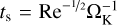$t_{\text{s}}={\mathrm{Re}}^{-1/2}{\text{ΩK}}_{-1}^{}$ is the small eddy turnover time. Using the same functional form as for the growth rate Eq. 29, but now from 0 to 1 instead of -1 to 1, we define $$p_{\text{turb}.1}:=\frac{1}{2}\left(1-\frac{{\left(f_{\text{turb}.1}^{\text{turb}.}\right)}^4-1}{{\left(f_{\text{turb}.1}^{\text{turb}.2}\right)}^4+1}\right).$$(C.2)

This expression is approaching 0 if τ_max < 5t_s and 1 if τ_max > 5t_s.

We apply a very similar function to the transition from the drift-dominated regime to the turbulence-dominated regime. We define $$f_{\text{drift }}^{\text{turb }}=\frac{\text{Δ}{v}_{\text{turb }}}{\text{Δ}{v}_{\text{drift }}}\{\begin{array}{ll}>1\hfill & \text{ turbulence dominated }\hfill \\ <1\hfill & \text{ drift dominated }\hfill \end{array},$$(C.3)

where ∆v_turb is the turbulent collision velocity. We define $$p_{\text{drift }}:=\frac{1}{2}\left(1-\frac{{\left(f_{\text{drift }}^{\text{turb }}\right)}^6-1}{{\left(f_{\text{drift }}^{\text{turb }}\right)}^6+1}\right).$$(C.4)

where we found that a slightly steeper transition fits better with the results of local coagulation simulations.

Finally, we have to introduce the transition from growth to fragmentation. For this, we chose a steeper transition, following $$p_{\text{frag }}=\exp \left[-{\left(5\left(\min \left(\frac{\text{Δ}{v}_{\text{tot }}}{v_{\text{frag }}},1.0\right)-1.0\right)\right)}^2\right],$$(C.5)

which ensures that the equilibrium size distribution is reached on a fast enough timescale.

Appendix D Flux-limited dust diffusion

In order to avoid unrealistically large diffusion fluxes in the presence of strong gradients in the dust-to-gas ratio, we introduce a flux limiter that is conceptually identical to the one by Levermore & Pomraning (1981), which was used by Stammler & Birnstiel (2022). Without the flux limiter, the diffusion flux is given by $$F_{\text{diff}}=-D{\text{Σ}}_{\text{g}}\mathbf{\nabla }\epsilon .$$(D.1)

The transport velocity shall however not be larger than the turbulent velocities that drive the diffusion, meaning the maximum allowed flux is $$F_{\text{diff},\text{max}}:=v_{\text{turb }}\epsilon {\text{Σ}}_{\text{g}}=\frac{\sqrt{\delta }{c}_{\text{s}}}{1+{\text{St}}^2}\epsilon {\text{Σ}}_{\text{g}}.$$(D.2)

The flux limiter is now defined via $${\lambda }_{\lim }=\frac{1+\chi }{1+\chi +{\chi }^2},$$(D.3)

where $$\chi =\frac{F_{\text{diff }}}{F_{\text{diff},\text{max}}},$$(D.4)

is the ratio of the diffusion flux and the maximum flux. The limited flux is then given by $$F_{\text{diff},\text{lim}}={\lambda }_{\text{lim}}{F}_{\text{diff}}.$$(D.5)

Note that although the flux is a vector (with components for each direction), all operations here are component-wise. In PLUTO, we define all quantities in the above equations at the cell interfaces.

Appendix E Calibrations and test simulations without diffusion

Here, we present the same calibration and test simulations shown in the main part of this article, but now without dust diffusion (δ = 0).

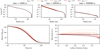Fig. E.1 Comparison between DustPy and our model in a setup without dust diffusion and with different drift calibration factors fdrift. Solid lines show the results of our TriPoD calibration runs and dashed lines show the respective DustPy simulation, to which we calibrate our model. The upper row shows a timeseries of the dust column density evolution in three snapshots. In the lower row, we show the mass evolution and the errors with respect to the full coagulation model DustPy. For a factor of fdrift = 0.8, the mass evolution of the full coagulation model is well reproduced by our three-parameter model.

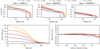Fig. E.2 Comparison between DustPy and our model in setups with different stellar masses without dust diffusion. Solid lines show the results of our TriPoD simulations and dashed lines show the respective DustPy simulations. The upper row shows a time series of the dust column density evolution in three snapshots. In the lower row, we show the mass evolution and the errors with respect to the full coagulation model DustPy.

References

All Tables

All Figures

Fig. 1 Comparison between the full coagulation model DustPy (upper row, 171 dust fluids) and our new three-parameter power-law prescription TriPoD, which we implemented in the PLUTO code (two dust fluids). We show two snapshots of the one-dimensional disk models in the first two panels in each row. The third panel shows the local dust size distribution of the respective model at 10 au for both snapshots. The light grid in the background represents size distribution power laws with n(a) ∝ a−3.5 and n(a) ∝ a−3.0.

In the text

Fig. 2 Typical size distributions in regions of a protoplanetary disk model that are either turbulence-dominated (dark red lines) or drift- dominated (blue lines). Both regimes result in distinct power-law exponents of the distribution that we overplot as dashed lines. Assuming a power law as the overall shape of the distribution makes it possible to approximately describe it with only three parameters: The cutoff particle size amax and the two densities Σ0 (contained in the size interval [$a_{\min },\sqrt{a_{\max }{a}_{\min }}$) and Σɪ (contained in the size interval [$\sqrt{a_{\max }{a}_{\min }},a_{\max }$]). This approximation is the basis of our new dust coagulation model.

In the text

	Fig. 3 Parameter study for the factor f∆υ, which is the most important parameter for the growth rate calibration of our model. For this, we calculated the deviation between the mass-averaged particle size’s growth rate in DustPy and TriPoD. In the top row, we show models for different global values of f∆υ. It can be seen that f∆υ = 0.4 seems to fit the dust growth rate best.
In the text

Fig. 4 Parameter study for the factor s, which determines the steepness of the transition from sweep-up growth to coagulation-fragmentation equilibrium in Eq. (29). Heat maps show the deviation of the growth rate in TriPoD from the growth rate in DustPy. The lower row shows the average over the size dimension. The influence of a variation in s can be seen around the fragmentation limit, where a larger s corresponds to a steeper transition (fast growth close to the fragmentation limit), while a small s corresponds to a slower transition where growth rates decrease earlier and more slowly. The case of s = 3 has the overall best fit with the DustPy model.

In the text

Fig. 5 Comparison between DustPy and our model in a setup with dust diffusion (δ = 10−3) and with different drift calibration factors fdrift. Solid lines show the results of our TriPoD calibration runs and dashed lines show the respective DustPy simulation, to which we calibrate our model. The upper row shows a timeseries of the dust column density evolution in three snapshots. In the lower row, we show the mass evolution and the errors with respect to the full coagulation model DustPy. For a factor of fdrift = 0.8, the mass evolution of the full coagulation model is well reproduced by our three-parameter model.

In the text

Fig. 6 Test for the size reduction in planetary gaps. The dashed lines correspond to the maximum grain size of the respective model (see color bars for the model parameters), while the solid lines show the dust column density for each model. Thick black lines correspond to the respective DustPy simulation that we want to reproduce. The particle size is reduced on the dust depletion timescale when the large dust population makes up less than the critical fraction ƒcrit of the total dust density. We run these simulations to determine which value leads to the best agreement with the DustPy simulation.

In the text

Fig. 7 Comparison of the dust size distributions in three simulations with different stellar masses and different disk masses. The first row in each group depicts a DustPy simulation (full treatment of coagulation). The lower rows show the respective TriPoD simulations with the PLUTO code. Panels on the right depict the local dust size distributions at 10 au at both snapshots. The gray lines in the right panel follow power laws with q = −3.5 and q = −3.0.

In the text

Fig. 8 Comparison between DustPy and our model in setups with different stellar masses. Solid lines show the results of our TriPoD simulations and dashed lines show the respective DustPy simulations. The upper row shows a time series of the dust column density evolution in three snapshots. In the lower row, we show the mass evolution and the errors with respect to the full coagulation model DustPy.

In the text

Fig. 9 Comparison between a DustPy simulation and a PLUTO simulation with our TriPoD dust coagulation model of a protoplanetary disk with radially varying fragmentation velocity (see Eq. (59)). The left and center columns depict the global dust distribution at two different snapshots of the simulations, with the DustPy simulation in the top row and the TriPoD simulation at the bottom. The right plot shows the local dust size distributions in the second snapshot at the locations of the vertical lines of the same color in the central panel. The gray lines in the right panel follow power laws with q = −3.5 and q = −3.0.

In the text

Fig. 10 Comparison between a DustPy simulation and a PLUTO simulation with our TriPoD dust coagulation model in a protoplanetary disk with a pre-defined gap. We also show the particle sizes and dust column density profiles calculated with the old two-pop-py model as dotted lines. The plot on the right-hand side depicts the local dust size distributions at 5 au (within the gap) and at 8.5 au (at the pressure maximum), for two different snapshots. The gray lines in the right panel follow power laws with q = −3.5 and q = −3.0.

In the text

Fig. 11 Comparison between two-dimensional PLUTO simulations with the TriPoD coagulation model and with the two-pop-py model. Both simulations have the exact same gas density structure and are only distinguished by the applied dust coagulation model. The lower panels show the azimuthally averaged quantities. For the azimuthal averages, we have masked the region around the planet that has been marked with the white circle. The red line in the left panel shows the radial pressure gradient parameter $\eta =\frac{1}{2}{\left(\frac{H}{R}\right)}^2\frac{\partial \text{\hspace{0.17em}log\hspace{0.17em}}P}{\partial \text{\hspace{0.17em}log\hspace{0.17em}}R}$. It can be seen that in our simulation a weak second pressure maximum appears at ~20 au, which leads to strong trapping in the two-pop-py model (Birnstiel et al. 2012). This effect is much less pronounced if a polydisperse size distribution is considered as done in our TriPoD simulation, where the small dust population is less efficiently trapped.

In the text

Fig. E.1 Comparison between DustPy and our model in a setup without dust diffusion and with different drift calibration factors fdrift. Solid lines show the results of our TriPoD calibration runs and dashed lines show the respective DustPy simulation, to which we calibrate our model. The upper row shows a timeseries of the dust column density evolution in three snapshots. In the lower row, we show the mass evolution and the errors with respect to the full coagulation model DustPy. For a factor of fdrift = 0.8, the mass evolution of the full coagulation model is well reproduced by our three-parameter model.

In the text

Fig. E.2 Comparison between DustPy and our model in setups with different stellar masses without dust diffusion. Solid lines show the results of our TriPoD simulations and dashed lines show the respective DustPy simulations. The upper row shows a time series of the dust column density evolution in three snapshots. In the lower row, we show the mass evolution and the errors with respect to the full coagulation model DustPy.

In the text

References

- Andrews, S. M., Huang, J., Pérez, L. M., et al. 2018, ApJ, 869, L41 [NASA ADS] [CrossRef] [Google Scholar]
- Antonellini, S., Kamp, I., & Waters, L. B. 2023, A&A, 672, A92 [NASA ADS] [CrossRef] [EDP Sciences] [Google Scholar]
- Balbus, S. A., & Hawley, J. F. 1991, ApJ, 376, 214 [Google Scholar]
- Baraffe, I., Homeier, D., Allard, F., & Chabrier, G. 2015, A&A, 577, A42 [NASA ADS] [CrossRef] [EDP Sciences] [Google Scholar]
- Baruteau, C., Barraza, M., Pérez, S., et al. 2019, MNRAS, 486, 304 [Google Scholar]
- Benítez-Llambay, P., & Masset, F. S. 2016, ApJS, 223, 11 [Google Scholar]
- Benítez-Llambay, P., Krapp, L., & Pessah, M. E. 2019, ApJS, 241, 25 [Google Scholar]
- Bergez-Casalou, C., Bitsch, B., Kurtovic, N. T., & Pinilla, P. 2022, A&A, 659, A6 [NASA ADS] [CrossRef] [EDP Sciences] [Google Scholar]
- Binkert, F. 2023, MNRAS, 525, 4299 [NASA ADS] [CrossRef] [Google Scholar]
- Birnstiel, T. 2023, ARA&A, 62, 157 [Google Scholar]
- Birnstiel, T., Dullemond, C. P., & Brauer, F. 2009, A&A, 503, 5 [Google Scholar]
- Birnstiel, T., Dullemond, C. P., & Brauer, F. 2010, A&A, 513, A79 [NASA ADS] [CrossRef] [EDP Sciences] [Google Scholar]
- Birnstiel, T., Ormel, C. W., & Dullemond, C. P. 2011, A&A, 525, A11 [NASA ADS] [CrossRef] [EDP Sciences] [Google Scholar]
- Birnstiel, T., Klahr, H., & Ercolano, B. 2012, A&A, 539, A148 [NASA ADS] [CrossRef] [EDP Sciences] [Google Scholar]
- Birnstiel, T., Dullemond, C. P., Zhu, Z., et al. 2018, ApJ, 869, L45 [CrossRef] [Google Scholar]
- Blandford, R. D., & Payne, D. G. 1982, MNRAS, 199, 883 [CrossRef] [Google Scholar]
- Brauer, F., Dullemond, P., & Henning, T. 2008, A&A, 480, 859 [NASA ADS] [CrossRef] [EDP Sciences] [Google Scholar]
- Burn, R., Emsenhuber, A., Weder, J., et al. 2022, A&A, 666, A73 [NASA ADS] [CrossRef] [EDP Sciences] [Google Scholar]
- Charnoz, S., & Taillifet, E. 2012, ApJ, 753, 119 [NASA ADS] [CrossRef] [Google Scholar]
- Dominik, C., & Dullemond, C. P. 2024, A&A, 682, A144 [NASA ADS] [CrossRef] [EDP Sciences] [Google Scholar]
- Drążkowska, J., Li, S., Birnstiel, T., Stammler, S. M., & Li, H. 2019, ApJ, 885, 91 [Google Scholar]
- Drążkowska, J., Stammler, S. M., & Birnstiel, T. 2021, A&A, 647, 15 [Google Scholar]
- Drążkowska, J., Bitsch, B., Lambrechts, M., et al. 2023, in Protostars Planets VII, eds. S.-I. Inutsuka, Y. Aikawa, T. Muto, K. Tomida, & M. Tamura (San Francisco: ASPCS), 534, 717 [Google Scholar]
- Dubrulle, B., Morfill, G., & Sterzik, M. 1995, Icarus, 114, 237 [Google Scholar]
- Duffell, P. C. 2020, ApJ, 889, 16 [NASA ADS] [CrossRef] [Google Scholar]
- Dullemond, C. P., Birnstiel, T., Huang, J., et al. 2018, ApJ, 869, L46 [NASA ADS] [CrossRef] [Google Scholar]
- Emsenhuber, A., Mordasini, C., Burn, R., et al. 2021, A&A, 656, 69 [Google Scholar]
- Epstein, P. S. 1924, Phys. Rev., 23, 710 [Google Scholar]
- Estrada, P. R., & Cuzzi, J. N. 2008, ApJ, 682, 515 [Google Scholar]
- Fromang, S., & Nelson, R. P. 2009, A&A, 496, 597 [NASA ADS] [CrossRef] [EDP Sciences] [Google Scholar]
- Gárate, M., Delage, T. N., Stadler, J., et al. 2021, A&A, 655, 18 [Google Scholar]
- Guillet, V., Hennebelle, P., Pineau Des Forêts, G., et al. 2020, A&A, 643, 17 [Google Scholar]
- Güttler, C., Blum, J., Zsom, A., Ormel, C. W., & Dullemond, C. P. 2010, A&A, 513, A56 [Google Scholar]
- Huang, P., & Bai, X.-N. 2022, ApJS, 262, 11 [NASA ADS] [CrossRef] [Google Scholar]
- Kobayashi, H., Tanaka, H., & Okuzumi, S. 2016, ApJ, 817, 105 [NASA ADS] [CrossRef] [Google Scholar]
- Kolmogorov, A. N. 1941, Doklady Akademii Nauk SSSR, 30, 299 [Google Scholar]
- Kornet, K., Stepinski, T. F., & Rózyczka, M. 2001, A&A, 378, 180 [NASA ADS] [CrossRef] [EDP Sciences] [Google Scholar]
- Krijt, S., & Ciesla, F. J. 2016, ApJ, 822, 111 [NASA ADS] [CrossRef] [Google Scholar]
- Lau, T. C. H., Drążkowska, J., Stammler, S. M., Birnstiel, T., & Dullemond, C. P. 2022, A&A, 668, 170 [Google Scholar]
- Leiendecker, H., Jang-Condell, H., Turner, N. J., & Myers, A. D. 2022, ApJ, 941, 172 [NASA ADS] [CrossRef] [Google Scholar]
- Lenz, C. T., Klahr, H., Birnstiel, T., Kretke, K., & Stammler, S. 2020, A&A, 640, A61 [NASA ADS] [CrossRef] [EDP Sciences] [Google Scholar]
- Lesur, G., Ercolano, B., Flock, M., et al. 2023, in Protostars Planets VII, eds. S.-I. Inutsuka, Y. Aikawa, T. Muto, K. Tomida, & M. Tamura (San Francisco: ASPSC), 534, 465 [NASA ADS] [Google Scholar]
- Levermore, G. D., & Pomraning, G. C. 1981, ApJ, 248, 321 [NASA ADS] [CrossRef] [Google Scholar]
- Lichtenberg, T., Drążkowska, J., Schönbächler, M., Golabek, G. J., & Hands, T. O. 2021, Science, 371, 365 [NASA ADS] [CrossRef] [Google Scholar]
- Lombart, M., & Laibe, G. 2021, MNRAS, 501, 4298 [Google Scholar]
- Lombart, M., Hutchison, M., & Lee, Y. N. 2022, MNRAS, 517, 2012 [CrossRef] [Google Scholar]
- Lombart, M., Bréhier, C.-E., Hutchison, M., & Lee, Y.-N. 2024, MNRAS, 533, 4410 [CrossRef] [Google Scholar]
- Marchand, P., Guillet, V., Lebreuilly, U., & Mac Low, M. M. 2021, A&A, 649, A50 [NASA ADS] [CrossRef] [EDP Sciences] [Google Scholar]
- Marchand, P., Guillet, V., Lebreuilly, U., & Mac Low, M. M. 2022, A&A, 666, A27 [NASA ADS] [CrossRef] [EDP Sciences] [Google Scholar]
- Marchand, P., Lebreuilly, U., Mac Low, M. M., & Guillet, V. 2023, A&A, 670, A61 [NASA ADS] [CrossRef] [EDP Sciences] [Google Scholar]
- Mathis, J. S., Rumpl, W., & Nordsieck, K. H. 1977, ApJ, 217, 425 [Google Scholar]
- Mignone, A., Bodo, G., Massaglia, S., et al. 2007, ApJS, 170, 228 [Google Scholar]
- Muley, D., Fuksman, J. D. M., & Klahr, H. 2023, A&A, 678, A162 [NASA ADS] [CrossRef] [EDP Sciences] [Google Scholar]
- Nakagawa, Y., Nakazawa, K., & Hayashi, C. 1981, Icarus, 45, 517 [NASA ADS] [CrossRef] [Google Scholar]
- Nakagawa, Y., Sekiya, M., & Hayashi, C. 1986, Icarus, 67, 375 [Google Scholar]
- Öberg, K. I., Guzmán, V. V., Walsh, C., et al. 2021, ApJS, 257, 1 [CrossRef] [Google Scholar]
- Ormel, C. W., & Cuzzi, J. N. 2007, A&A, 466, 413 [NASA ADS] [CrossRef] [EDP Sciences] [Google Scholar]
- Ormel, C. W., Cuzzi, J. N., & Tielens, A. G. G. M. 2008, ApJ, 679, 1588 [NASA ADS] [CrossRef] [Google Scholar]
- Pascucci, I., Cabrit, S., Edwards, S., et al. 2023, in Protostars Planets VII, eds. S.-I. Inutsuka, Y. Aikawa, T. Muto, K. Tomida, & M. Tamura (San Francisco: ASPCS), 567 [Google Scholar]
- Pérez, L. M., Benisty, M., Andrews, S. M., et al. 2018, ApJ, 869, L50 [CrossRef] [Google Scholar]
- Pfeil, T., Cranmer, M., Ho, S., et al. 2022, in Machine Learning and the Physical Sciences workshop NeurIPS [Google Scholar]
- Pfeil, T., Birnstiel, T., & Klahr, H. 2023, ApJ, 959, 121 [NASA ADS] [CrossRef] [Google Scholar]
- Pinilla, P., Lenz, C. T., & Stammler, S. M. 2021, A&A, 645, A70 [NASA ADS] [CrossRef] [EDP Sciences] [Google Scholar]
- Powell, D., Murray-Clay, R., Pérez, L. M., Schlichting, H. E., & Rosenthal, M. 2019, ApJ, 878, 116 [NASA ADS] [CrossRef] [Google Scholar]
- Schlichting, H. E., & Sari, R. 2011, ApJ, 728, 68 [NASA ADS] [CrossRef] [Google Scholar]
- Simon, J. B., Blum, J., Birnstiel, T., & Nesvorný, D. 2022, Comets III (Tucson: University of Arizona Press) [arXiv:2212.04509] [Google Scholar]
- Smoluchowski, M. 1916, Phys. Z., 17, 557 [Google Scholar]
- Stammler, S. M., & Birnstiel, T. 2022, ApJ, 935, 35 [NASA ADS] [CrossRef] [Google Scholar]
- Stone, J. M., Tomida, K., White, C. J., & Felker, K. G. 2020, ApJS, 249, 4 [NASA ADS] [CrossRef] [Google Scholar]
- Tamfal, T., Drążkowska, J., Mayer, L., & Surville, C. 2018, ApJ, 863, 97 [NASA ADS] [CrossRef] [Google Scholar]
- Tsukagoshi, T., Nomura, H., Muto, T., et al. 2022, ApJ, 928, 49 [NASA ADS] [CrossRef] [Google Scholar]
- Tsukamoto, Y., & Okuzumi, S. 2022, ApJ, 934, 88 [NASA ADS] [CrossRef] [Google Scholar]
- Vorobyov, E. I., & Elbakyan, V. G. 2019, A&A, 631, A1 [NASA ADS] [CrossRef] [EDP Sciences] [Google Scholar]
- Vorobyov, E. I., Akimkin, V., Stoyanovskaya, O., Pavlyuchenkov, Y., & Liu, H. B. 2018, A&A, 614, A98 [NASA ADS] [CrossRef] [EDP Sciences] [Google Scholar]
- Vorobyov, E. I., Skliarevskii, A. M., Elbakyan, V. G., et al. 2019, A&A, 627, A154 [NASA ADS] [CrossRef] [EDP Sciences] [Google Scholar]
- Vorobyov, E. I., Matsukoba, R., Omukai, K., & Guedel, M. 2020, A&A, 638, A102 [NASA ADS] [CrossRef] [EDP Sciences] [Google Scholar]
- Weidenschilling, S. J. 1977, MNRAS, 180, 57 [Google Scholar]
- Weidenschilling, S. J. 1980, Icarus, 44, 172 [NASA ADS] [CrossRef] [Google Scholar]
- Wetherill, G. W., & Stewart, G. R. 1989, Icarus, 77, 330 [Google Scholar]
- Whipple, F. 1972, in From Plasma to Planet, ed. A. Evlius (New York: Wiley Interscience Division), 211 [Google Scholar]
- Youdin, A. N., & Goodman, J. 2005, ApJ, 620, 459 [Google Scholar]
- Zsom, A., Ormel, C. W., Güttler, C., Blum, J., & Dullemond, C. P. 2010, A&A, 513, A57 [NASA ADS] [CrossRef] [EDP Sciences] [Google Scholar]
- Zsom, A., Ormel, C. W., Dullemond, C. P., & Henning, T. 2011, A&A, 534, A73 [NASA ADS] [CrossRef] [EDP Sciences] [Google Scholar]
See https://stammler.github.io/dustpy/example_ice_lines.html for the corresponding DustPy setup.
All Tables
Stellar parameters and disk parameters for the simulations presented in this work.
Parameters of the one-dimensional simulations performed to calibrate the three-parameter model to the DustPy simulations.
Dust properties for the calibration runs (Sections 4.1 and 4.2) and the test simulations with different stellar masses Section 5.1.