© The Authors 2024

1 Introduction

The bodies in the Solar System are highly depleted in carbon, compared to the Sun. Figure 1 shows the carbon fraction, f_c, of the Solar System bodies, where the carbon fraction, f_c, is defined by the mass fraction of refractory carbon relative to the total refractory components (for details, see Binkert & Birnstiel 2023). The carbon fractions for the Sun, interstellar medium (ISM) dust, comets, and interplanetary dust particles (IDPs) are calculated from the C/Si atomic ratio in each body (Binkert & Birnstiel 2023). The carbon fractions of chondrite meteorites are calculated using the mass fraction of insoluble carbon contents, normalized by their matrix volume (Alexander et al. 2007, see below). While the fc values of ISM dust, IDPs, and comets are comparable to the solar value, the fc values of the bulk silicate Earth (BSE), which is the mantle and crust without the core of the Earth, is lower by 4 orders of magnitudes than the solar value.

The Earth’s mass is not large enough to accrete large amounts of gas. If all carbon carriers are in volatile forms such as CO, CO₂, or CH₄, it is reasonable that carbon components were not in the Earth’s building blocks (pebbles and planetesimals) near the Earth’s orbit, resulting in the significant carbon depletion in the Earth. However, about half of the carbon carriers in molecular clouds and primordial comets are likely to be in refractory forms. In the ISM, radio spectrographic observations suggest that ~60% of the cosmic carbon exists as highly refractory materials including six-membered rings such as amorphous hydrocarbons, polycyclic aromatic hydrocarbons (PAHs), or graphites (Savage & Sembach 1996). They would survive until they arrive at the hot regions with T ≳ 1000 K where they are destroyed by pyrolysis or oxidation by OH (e.g., Finocchi et al. 1997; Gail & Trieloff 2017). On the other hand, Fomenkova (1997, 1999) argued that about 60% of all solid carbonaceous materials (including less refractory carbon solids) in the comet Halley are “complex organics” such as a mixture of kerogen and insolvable organic matter (IOM) that survive until they are pyrolyzed at T ~ 500 K. These organics are often called “refractory organics”. However, because they are much less refractory than amorphous hydrocarbons, graphites, and PAHs, here we refer to them simply as “complex organics” to avoid confusion. We summarize the disk mid-plane temperature required for the destruction of each of the refractory carbon materials (T_des) in Table 1, which shows that most of the refractory carbon components should be in dust forms around Earth’s orbit. If Earth’s building blocks originated from the same carbon carriers as in molecular clouds, their compositions should be similar to those of ISM dust and comets with the removal of volatile carbon gas that would have been sublimated inside their ice lines. The carbon reduction due to the sublimation of volatile carbon gas should only be on the level of a factor of a few (and certainly not four orders of magnitude).

Assuming that carbon in the Earth’s mantle or crust may have been partitioned to its core in the magma ocean stage (Sakuraba et al. 2021), f_c values of the bulk Earth could be higher by 1–2 orders of magnitudes than that of BSE. However, even in that case, the Earth is still depleted in carbon by more than two orders of magnitude from the solar value. Remarkably, even carbonaceous chondrites (CC) are depleted in carbon by more than one order of magnitude from the Sun.

The “bulk” values (rather than matrix-normalized values) of f_c for enstatite chondrites (ECs) and ordinary chondrites (OCs) are in between “bulk Earth” and CC, monotonically increasing with the orbital radii of the Earth and the inferred parent asteroids (e.g., Bergin et al. 2015; Binkert & Birnstiel 2023). However, ECs and OCs include substantial chondrules that are carbon-free. The carbons there might have been lost during the flash heating (Gail & Trieloff 2017). It would be more appropriate to normalize the carbon fraction by the matrix volumes (Alexander et al. 2007), as in Fig. 1; the normalized fc in ECs, OCs, and CC would be similar independent of the heliocentric radius.

These observational data strongly suggest that carbons in the refractory forms should have been destroyed by some mechanism in the inner Solar System. The question of what specific mechanism is at work remains a mystery.

Carbon depletion may have also occurred in many exoplan-etary systems. About 25 to 50% of white dwarfs (WDs) are polluted by heavy elements (metals) such as Fe, Si, O, and C in their photospheres (e.g., Zuckerman et al. 2003, 2010; Koester et al. 2014; Hollands et al. 2017); however, these metals should quickly turn to sediment to the WDs’ interiors in the WD’s strong gravitational fields (Paquette et al. 1986; Koester 2010). This suggests that rocky planets or asteroids fall onto the host WDs through accretion disks (e.g., Okuya et al. 2023, and references therein), implying that the observed metal abundance should reflect the bulk compositions of the rocky bodies and it shows that C/Si is distributed from the solar value down to the BSE value (Zuckerman & Young 2018). The carbon depletion problem is not only an issue in the Solar System but also in exoplanetary systems.

Oxidation destroys amorphous hydrocarbons, PAHs, and graphites. When an oxygen atom collides with dust, a carbon atom is stripped to form a gaseous CO molecule. Lee et al. (2010) showed that enough amounts of hot oxygen atoms to oxidize graphite are produced by far-ultraviolet (FUV) irradiation in an upper layer over the disk photo-surface. The oxidation timescale of graphite is also applied for amorphous hydrocarbons and PAHs. Amorphous hydrocarbons may also be directly destroyed by FUV photons (Anderson et al. 2017); small hydrocarbons are released from the surface of an amorphous hydrocarbon particle that contains 10⁶ or more C atoms (Alata et al. 2014, 2015). In this paper, we refer to this destruction as “photolysis”.

The complex organics are thermally destroyed at T_des ~ 500 K (Table 1), which we call “pyrolysis”. Although they are converted to gas molecules, half of pyrolysis products may be hydrocarbons with T_des ≳ 1000 K (e.g., Chyba et al. 1990; Gail & Trieloff 2017). The experiments of Nakano et al. (2003) showed that remnants of pyrolysis can exist even in regions where the temperature exceeds 700 K, although the mass fraction of the remnants is unclear. Bergin et al. (2015) and Li et al. (2021) assumed only complex organics as a source of refractory carbons in ISM to propose that migration of their sublimation line (“soot line”) solves the carbon depletion problem in the inner Solar System. However if the remnants of the pyrolysis are hydrocarbons, the question of how hydrocarbons are destroyed must be discussed, even if the ISM refractory carbons do not include the highly refractory materials: hydrocarbons, PAHs, or graphites.

Klarmann et al. (2018) and Binkert & Birnstiel (2023) studied the carbon depletion in the inner Solar System, through Eulerian diffusion and advection simulations with the two-components fluid approximation of disk gas and dust. Klarmann et al. (2018) calculated the destruction of hydrocarbon particles due to oxidization and FUV photolysis, taking into account the dust drift and diffusion due to disk gas accretion and turbulence. They concluded that it is difficult to explain the observed carbon depletion because the dust radial drift timescale is much shorter than the timescale required to destroy most of the refractory carbon particles there.

Binkert & Birnstiel (2023) considered both the photolysis of amorphous hydrocarbons and pyrolysis of complex organics. They suggested that the carbon depletion could be explained if the FU Ori-type outburst sublimates all of the complex organ-ics and if the dust surface density and the optical depth for FUV are low enough to promote photolysis. However, it is not clear that the FU Ori-type outburst events occurred in the proto-Solar System and enough amount of the irradiated dust particles stay to be building blocks of the inner Solar System bodies. Furthermore, they assumed most of the refractory carbons are complex organics. If their conversion to amorphous hydrocarbons is taken into account, their conclusion may change.

These previous studies assumed that dust is composed only of silicates and carbon materials. However, beyond the snow line, H₂O components are added. Conventional results from experiments and numerical simulations suggested that ice may be stickier than silicate (e.g., Blum & Wurm 2000; Zsom et al. 2011; Wada et al. 2011), and icy particles grow to larger sizes than silicate particles. Here, we assume that carbonaceous solid materials move with silicate particles. If the icy pebbles envelop many small silicate particles, the silicate particles are released by sublimation of the icy mantle. Because of their small size, they are coupled to gas and piled up like traffic jam near the snow line, which may result in rocky planetesimal formation (e.g., Saito & Sirono 2011; Ida & Guillot 2016; Ida et al. 2021) and an enhancement of the crystalline to amorphous ratio of silicates even beyond the snow line (Okamoto & Ida 2022).

These previous studies did not consider the effect of the vertical temperature profile on the particle motions, because they estimated the vertical diffusion timescale by using the mid-plane temperature of the disk. However, in the optically thin upper layer, the local gas temperature is higher than in the mid-plane. It enhances turbulent motions there to lift particles more. At the same time, the lower gas density weakens the gas drag coupling, which suppresses particle stirring. Because oxidation and photolysis are regulated by how much the particles are stirred up to the upper layer, it is important to include the above effects. Our Lagrangian particle tracking method can more easily incorporate these effects than the Eulerian method adopted by the previous studies.

In this paper, we investigate the effect of the different sizes between icy and silicate particles and that of the vertical temperature profile on the carbon depletion problem. We adopt a global 3D Monte Carlo simulation (Ciesla 2010; Okamoto & Ida 2022) to calculate the radial drift and turbulent diffusion motions of solid particles in a disk and the chemical reactions (Ishizaki et al. 2023) such as photolysis in the upper FUV-exposed layer by tracking motions of individual particles. Because our model also calculates the particle size evolution due to coagulation and fragmentation, the pebble flux decay is consistently calculated.

In Sect. 2, we describe our Monte Carlo methods for particle motions and refractory carbon destruction models. In Sect. 3, we show the simulation results. The carbon fraction drops off inside the snow line by two or more orders of magnitude from the solar value in a fiducial case. We also investigate the dependence on simulation parameters. In Sect. 4, we compare the simulation results to the observational data. Section 5 presents our conclusions.

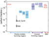Fig. 1 Carbon fraction of Solar System bodies, where the carbon fraction, fc, is defined by the mass fraction of carbon in the sum of solid carbon and the silicates. For ISM dust, comets, and IDPs, this fraction is calculated from the C/Si atomic ratio (Matrajt et al. 2005; Bardyn et al. 2017; Bergin et al. 2015; Binkert & Birnstiel 2023, and references therein). For comparison, we also plot the “Sun” values (fc ≃ 0.25), which refer to hypothetical dust with solar C/Si. The fractions of chondrites are normalized by the matrix volume of each chondrite (see the main text). While Bergin et al. (2015) and Binkert & Birnstiel (2023) showed fc fraction monotonically decreases as the decrease in the heliocentric radius decreases, the matrix-normalized fc of chondrites may be independent of the distance. The uncertainties of chondrites’ fc values come from the variation among each chondrite. The very low fc of BSE and “bulk Earth” are also discussed in the main text.

2 Method

2.1 Disk model

We assumed a self-similar protoplanetary gas disk (Hartmann et al. 1998) with characteristic radius r_disk = 100 au. At r ≪ r_disk, the disk gas accretion rate (Ṁ_g) is independent of r (steady accretion) and Ṁ_g decays as ∝ (1 + t/t_disk)^−3/2, where t_disk ≃ 10⁷(a/10⁻³)⁻¹(r_disk/100 au)yr. We assumed the conventional gas accretion model due to turbulent diffusion and do not consider disk-wind driven accretion, for simplicity. The gas surface density is given by $$\begin{array}{l}{\text{Σ}}_{\text{g}}=\frac{{\dot{M}}_{\text{g}}\mu m_{\text{H}}{\text{Ω}}_{\text{K}}}{3\pi \alpha k_{\text{B}}{T}_{\text{mid}}}\\ \simeq 1200\left(\frac{{\dot{M}}_{\text{g}}}{{10}^{-8}{M}_{\odot }/\text{yr}}\right){\left(\frac{\alpha }{{10}^{-3}}\right)}^{-1}{\left(\frac{T_{\text{mid }}}{300 \text{K}}\right)}^{-1}{\left(\frac{r}{1\text{\hspace{0.17em}au}}\right)}^{-3/2} \text{g}/{\text{cm}}^2,\end{array}$$(1)

where α is a parameter of turbulent strength and Ω_K is Keplerian frequency.

The hydrostatic local gas density is given by $${\rho }_{\text{g}}=\frac{{\text{Σ}}_{\text{g}}}{\sqrt{2\pi }{H}_{\text{g}}}\text{\hspace{0.17em}exp\hspace{0.17em}}\left(-\frac{z^2}{2H_{\text{g}}^2}\right),$$(2)

where H_g is the disk gas scale height. The disk aspect ratio is $$h_{\text{g}}=\frac{H_{\text{g}}}{r}=0.034{\left(\frac{T}{300 \text{K}}\right)}^{1/2}{\left(\frac{r}{1\text{\hspace{0.17em}au}}\right)}^{1/2}.$$(3)

We set the gas disk temperature distribution as follows. We calculate the mid-plane temperature $T_{\text{mid}}\text{\hspace{0.17em}by\hspace{0.17em}}{T}_{\text{mid}}^4=T_{\text{vis}}^4+T_{\text{irr}}^4$, where T_vis and T_irr are the temperature determined by viscous heating and irradiation, respectively. The viscous heating temperature with the opacity given by Bell & Lin (1994): T_vis = min(T_vis,ice, max(T_vis,eva, T_vis,sil)), where T_vis,ice and T_vis,sil are the temperatures with ice and silicate dust opacity, respectively, and T_viseva is that with the opacity for a transition from ice to silicate due to the evaporation of ice, which are given by $$T_{\text{vis, ice }}=1141{\left(\frac{{\dot{M}}_{\text{g}}}{{10}^{-8}{M}_{\odot }/\text{yr}}\right)}^{2/3}{\left(\frac{\alpha }{{10}^{-3}}\right)}^{-1/3}{\left(\frac{r}{1\text{\hspace{0.17em}au}}\right)}^{-3/2} \text{K}.$$(4) $$T_{\text{vis},e\text{va}}=270{\left(\frac{{\dot{M}}_{\text{g}}}{{10}^{-8}{M}_{\odot }/\text{yr}}\right)}^{1/6}{\left(\frac{\alpha }{{10}^{-3}}\right)}^{-1/12}{\left(\frac{r}{1\text{\hspace{0.17em}au}}\right)}^{-3/8} \text{K},$$(5) $$T_{\text{vis},\text{sil}}=433{\left(\frac{{\dot{M}}_{\text{g}}}{{10}^{-8}{M}_{\odot }/\text{yr}}\right)}^{4/9}{\left(\frac{\alpha }{{10}^{-3}}\right)}^{-2/9}{\left(\frac{r}{1\text{\hspace{0.17em}au}}\right)}^{-1} \text{K}.$$(6)

On the other hand, the temperature by irradiation is set to (Oka et al. 2011; Ida et al. 2016) $$T_{\text{irr}}=150{\left(\frac{r}{1\text{\hspace{0.17em}au}}\right)}^{-3/7} \text{K}.$$(7)

The transition between T_vis and T_irr occurs at $$r_{\text{vis-irr }}=6.6{\left(\frac{{\dot{M}}_{\text{g}}}{{10}^{-8}{M}_{\odot }/\text{yr}}\right)}^{28/45}{\left(\frac{\alpha }{{10}^{-3}}\right)}^{-14/45}\text{au}.$$(8)

Figure 2 shows the gas surface density and the mid-plane temperature distributions in the fiducial run.

The vertical temperature distribution is set as follows. In the upper optically thin FUV-exposed layer (at |z| ≳ (3–4) H_g), the temperature is generally higher than near the mid-plane, which is given by (Klarmann et al. 2018) $$T_{\text{FUV}}=750{\left(\frac{r}{1\text{\hspace{0.17em}au}}\right)}^{-3/5} \text{K}.$$(9)

We connect T_FUV with T_mid in the mid-plane as $$T_{ɀ}^4=T_{\text{mid }}^4\left(1-\exp \left(-{\tau }_{\text{FUV},ɀ}\right)\right)+T_{\text{FUV}}^4\exp \left(-{\tau }_{\text{FUV},ɀ}\right),$$(10)

where τ_FUV,z is the vertical optical depth for FUV given by Eq. (44). Figure 3 shows T_z at 1 au.

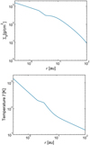Fig. 2 Gas surface density, Σg, (upper panel) and the mid-plane temperature (lower panel) in the fiducial run.

2.2 Monte Carlo simulation

2.2.1 Representative refractory carbons

We considered the two types of refractory carbons: amorphous hydrocarbon as the highly refractory materials and complex organics as modest refractory materials, although, in many simulation sets, we considered only amorphous hydrocarbons by the reason in Sect. 1. Because graphites and PAHs would have similar destruction temperatures (Table 1) and, in an observational sense, it is not clear what fraction of interstellar carbon exists in individual forms of refractory materials, the highly refractory carbons are represented by the amorphous hydrocarbons (in this paper). We assumed that amorphous hydrocarbon particles are destructed by the photolysis and/or oxidation in the FUV-exposed layer.

Fig. 3 Vertical temperature profile at 1 au given by Eq. (10).

2.2.2 Photolysis and oxidation

When the carbonaceous particles are lifted to the upper layer by turbulence, the particles are assumed to be “photodegraded” or “oxidized”. In this paper, “photolysis” is defined as the reaction that small hydrocarbon volatile molecules such as methane are released from the surface of the amorphous hydrocarbon particles by FUV, as suggested by Alata et al. (2015), and “oxidation” means the reaction that single C atoms are removed from the carbon particle surface by the collisions with oxygen atoms as gaseous carbon monoxide molecules. Since the oxygen atoms should be abundant only in the upper layer of the disk (e.g., Lee et al. 2010), we calculated the oxidation rate only when the particle exists in the FUV-exposed layer (see Sect. 2.4.1). Although oxidation by OH could occur (e.g., Bauer et al. 1997; Finocchi et al. 1997), the abundance of OH is uncertain near the mid-plane and the oxygen atoms are more abundant than OH in the FUV-exposed layer (Lee et al. 2010). Accordingly, we did not consider oxidation by OH. The rates of photolysis and oxidation are described in Sects. 2.4.2 and 2.4.3.

When the Stokes number (St), which is defined by the stopping time due to gas drag scaled by the inverse of local Kepler frequency, is smaller than the viscosity parameter α for the released and piled-up silicate particles at the snow line (and when St > α for icy pebbles), the silicate particles are stirred up more highly than the icy pebbles. In this case, the piled-up silicate particles block FUV radiation from the central star to the region beyond the snow line, which is also known as the “shadow area” (e.g., Ueda et al. 2019; Ohno & Ueda 2021). Therefore, we assumed that amorphous hydrocarbons are not destroyed outside the snow line.

2.2.3 Fragmentation limit velocity

In the fiducial case, we adopted the conventional fragmentation limit velocity for ice particles as υ_frag,ice = 10m/s (e.g., Wada et al. 2013; Gundlach & Blum 2015) and for silicate particles as υ_frag,sil = 1m/s (e.g., Wada et al. 2013). We note that this conventional notion is now challenged by new experiments and recent observations of the protoplanetary disks (see below). In this fiducial case, silicate particles cannot grow enough and stay small.

We assumed that amorphous hydrocarbons are included in the silicate particles. Outside the snow line, water vapor condenses on the small silicate particles and these ice-enveloped particles would stick together according to the larger fragmentation velocity for ice to form relatively large aggregates, known as “icy pebbles”. When the particles pass inward the snow line, the icy mantle evaporates, and the small silicate particles inside the icy pebbles are released. As we will show later, the released silicate particles are piled up because they are coupled more strongly to disk gas than the icy pebbles are. The sizes of the silicate particles and the icy pebbles are calculated automatically by the model considering the fragmentation limit (Sect. 2.2.5).

Realistic fragmentation velocities of the icy and silicate particles remain uncertain. As mentioned above, although the previous studies showed that icy particles can stick easier than silicates, recent experiments showed that the stickiness of icy particles is similar to that of silicates (e.g., Musiolik & Wurm 2019; Schräpler et al. 2022). Furthermore, recent observations could also show that the size of mass-dominant icy particles is ≲ 1 mm in outer regions of protoplanetary disks, which corresponds to the fragmentation velocity of icy particles of ≲1 m/s (Kataoka et al. 2015; Ueda et al. 2024). However, even if the fragmentation velocities of silicate and icy particles are similar to each other, the icy particles could become larger by recondensation of water vapor near the snow line (Ros et al. 2019), which is not incorporated in this study. In this case, the results can be similar to the fiducial case. A more detailed investigation is left for future work.

We set the fragmentation limit velocities for amorphous hydrocarbons to be the same as silicate particles to highlight the effect of the fragmentation velocity difference, for simplicity. We note that the stickiness of carbonaceous materials is also unclear. Although some previous studies suggested complex organics on the particle’s surface make the silicate particle stickier (e.g., Kudo et al. 2002; Homma et al. 2019), a recent experiment showed that their stickiness is similar to dry silica dust (Bischoff et al. 2020).

2.2.4 Orbital evolution of particles

In order to follow the orbital evolution of silicate particles described in Sect. 2.2.3, we employed the 3D Monte Carlo simulation method for radial drift and diffusion of silicate particles developed by Ciesla (2010, 2011). The surface density evolution of the icy and silicate particles is determined by the concentration equation: $$\frac{\partial {\text{Σ}}_{\text{d}}}{\partial t}=\frac{1}{r}\frac{\partial }{\partial r}\left[r{\text{Σ}}_{\text{d}}\left(v_r-\frac{D}{{\text{Σ}}_{\text{d}}/{\text{Σ}}_{\text{g}}}\frac{\partial }{\partial r}\left(\frac{{\text{Σ}}_{\text{d}}}{{\text{Σ}}_{\text{g}}}\right)\right)\right],$$(11)

where Σ_d is the surface density of the icy and silicate particles, D is their diffusivity, and υ_r is their radial drift velocity. The vertical advection-diffusion equation is given by $$\frac{\partial {\rho }_{\text{d}}}{\partial t}=\frac{\partial }{\partial ɀ}\left({\rho }_{\text{g}}D\frac{\partial }{\partial ɀ}\left(\frac{{\rho }_{\text{d}}}{{\rho }_{\text{g}}}\right)\right)-\frac{\partial }{\partial ɀ}\left({\rho }_{\text{d}}{v}_{ɀ}\right),$$(12)

where ρ_d is the local spatial density of solid particles. In a steady accretion disk, the changes in the positions in Cartesian coordinates (x, y, z) of each particle after the timestep δt are given by $$\delta x=v_r\times \frac{x}{r}\delta t+{ℛ}_x\sqrt{6D\left(x^{\prime }\right)\delta t},$$(13) $$\delta y=v_r\times \frac{y}{r}\delta t+{ℛ}_y\sqrt{6D\left(y^{\prime }\right)\delta t},$$(14) $$\delta ɀ=\left[v_{ɀ}+\frac{1}{{\rho }_{\text{g}}}\frac{\partial \left(D{\rho }_{\text{g}}\right)}{\partial ɀ}\right]\delta t+{ℛ}_{ɀ}\sqrt{6D\left({ɀ}^{\prime }\right)\delta t},$$(15)

where δt is given by the inverse of the local Keplerian frequency, $\delta t={\text{Ω}}_{\text{K}}^{-1}$, and x′, y′, and z′ are given by $$x^{\prime }=x+\frac{1}{2}\frac{\partial D}{\partial x}\delta t;y^{\prime }=y+\frac{1}{2}\frac{\partial D}{\partial y}\delta t;{ɀ}^{\prime }=ɀ+\frac{1}{2}\frac{\partial D}{\partial ɀ}\delta t.$$(16)

The first and second terms on the right-hand sides represent the advection and diffusion. In the diffusion terms, 𝓡_x, 𝓡_y, and 𝓡_z are independent random numbers in a range of [−1,1] with a root mean square of $1/\sqrt{3}$. We set the particles’ dif-fusivity considering collective effect as (Hyodo et al. 2021; Okuya et al. 2023) $$D=\frac{\text{Λ}}{1+{\text{Λ}}^2{\text{St}}^2}v,$$(17)

where v is the gas turbulent viscosity given by $$v=\alpha h_{\text{g}}^2{r}^2{\text{Ω}}_{\text{K}},$$(18)

and St is the Stokes number given by $$\text{St}=\{\begin{array}{ll}\frac{{\rho }_{\text{bulk }}s}{{\rho }_{\text{g}}{v}_{\text{th }}}{\text{Ω}}_{\text{K}}\hfill & \left[s\le \frac{9}{4}{\lambda }_{\text{mip }}:\text{ Epstein }\right],\hfill \\ \frac{{\rho }_{\text{bulk }}s}{{\rho }_{\text{g}}{v}_{\text{th }}}\frac{4s}{9{\lambda }_{\text{mfp}}}{\text{Ω}}_{\text{K}}\hfill & \left[s\ge \frac{9}{4}{\lambda }_{\text{mfp}}:\text{ Stokes }\right],\hfill \end{array}$$(19)

where $v_{\text{th}}=\sqrt{8/\pi }{c}_s,c_s$ is the sound speed of gas, λ_mfp is the mean free path of gas, Λ = (1 + ρ_d/ρ_g)⁻¹, and ρ_buik is the bulk density of the particle, which is assumed to be 3.0 g/cm³ for the silicate particles and 1.5 g/cm³ for icy pebbles.

Because we have adopted a disk temperature model where T is raised at |z| ≳ a few H_g (Fig. 4), we chose to adopt a vertical diffusivity that is calculated by local temperature. On the other hand, because most of the particles should be within the gas scale height, we set the radial diffusivity calculated by the mid-plane temperature without a vertical dependency. In this case, the radial dependence of diffusivity can be neglected in Eq. (16). In contrast, D can change significantly for z → z′ due to the steep increase or decrease of the temperature, as shown in Fig. 3. Thus, we can assume D(x′) ~ D(x) and D(y′) ~ D(y).

The radial drift velocity due to gas drag is given by (Ida & Guillot 2016; Schoonenberg & Ormel 2017) $$v_r\simeq -\frac{\text{Λ}}{1+{\text{Λ}}^2{\text{St}}^2}\left(2\text{Λ}\mathrm{St}\eta v_{\text{K}}+u_v\right),$$(20)

where υ_K is the local Keplerian velocity, u_v is the disk gas (inward) accretion velocity given by $u_v=3v/2r=\left(3\alpha h_{\text{g}}^2/2\right)v_{\text{K}}$, and η is the degree of deviation of the gas rotation angular velocity Ω from the Keplerian one, given by $$\eta \equiv \frac{{\text{Ω}}_{\text{K}}-\text{Ω}}{{\text{Ω}}_{\text{K}}}=-\frac{1}{2}\frac{d\ln P}{d\ln r}{h}_{\text{g}}^2=C_{\eta }{h}_{\text{g}}^2.$$(21)

For simplicity, we take C_η = 11/8 for T ∝ r^−1/2. The vertical advection velocity υ_z is given by (Ciesla 2010): $$v_{ɀ}=-\frac{\text{St}}{1+\text{St}}\text{Ω}ɀ.$$(22)

Therefore, Eqs. (13) to (15) can be rewritten as $$\delta x=-\frac{\text{Λ}}{1+{\text{Λ}}^2{\text{St}}^2}\left[2\text{Λ}{C}_{\eta }\text{St}+\frac{3}{2}\alpha \right]h_{\text{g}}^{2}x+{ℛ}_x\sqrt{\frac{6\alpha \text{Λ}}{1+{\text{Λ}}^2{\text{St}}^2}}{h}_{\text{g}}r,$$(23) $$\delta y=-\frac{\text{Λ}}{1+{\text{Λ}}^2{\text{St}}^2}\left[2\text{Λ}{C}_{\eta }\text{St}+\frac{3}{2}\alpha \right]h_g^{2}y+{ℛ}_y\sqrt{\frac{6\alpha \text{Λ}}{1+{\text{Λ}}^2{\text{St}}^2}}{h}_{g}r,$$(24) $$\delta z=-\left(\frac{\text{St}}{1+\text{St}}+\alpha \right)ɀ+{ℛ}_{ɀ}\sqrt{\frac{6\alpha \text{Λ}}{1+{\text{Λ}}^2{\text{St}}^2}}{h}_{\text{g}}\left({ɀ}^{\prime }\right)r.$$(25)

In our simulation, at every timestep, we calculated the instantaneous surface and local densities of solids (icy and silicate particles) from the super-particle distribution to evaluate size growth and collective effect. The solid surface density at r is given with the number of super-particles, ∆N_r, in the radial width of ∆r around r given by $${\text{Σ}}_{\text{d}}=\frac{m\text{\hspace{0.17em}Δ}{N}_r}{2\pi r\text{Δ}r}=\frac{m\text{\hspace{0.17em}Δ}{N}_r}{2\pi r^2\times 2.3\left(\text{Δ\hspace{0.17em}}{\log }_{10}r\right)}.$$(26)

where m is the super-particle mass. The solid local density at r and z is calculated by the number of super-particles ∆N_r,z in the radial and vertical width of ∆r and ∆z, given by $${\rho }_{\text{d}}=\frac{m\text{Δ}{N}_{r,ɀ}}{2\pi r\text{Δ}r\times 2\text{Δ}ɀ}=\frac{m\text{Δ}{N}_{r,ɀ}}{4\pi r^2\times 2.3\left(\text{Δ\hspace{0.17em}}{\log }_{10}r\right)\text{Δ}ɀ}.$$(27)

When the initial state of the surface density of particles is given by ∑_d = Z₀∑_g, the initial number of particles in each cell ∆N_r,0 is given by $$\text{Δ}{N}_{r,0}=\frac{Z_0{\text{Σ}}_{\text{g}}\times 4.6\pi r^2\left(\text{Δ\hspace{0.17em}}{\log }_{10}r\right)}{m}$$(28) $$\simeq 81\left(\frac{Z_0}{0.01}\right)\left(\frac{\text{Δ\hspace{0.17em}}{\log }_{10}r}{0.05}\right)\left(\frac{{\text{Σ}}_{\text{g}}}{1000 \text{g}/{\text{cm}}^2}\right){\left(\frac{m}{{10}^{-8}{M}_{\odot }}\right)}^{-1}{\left(\frac{r}{1\text{\hspace{0.17em}au}}\right)}^2.$$(29)

We summarize the simulation parameters in Table 2.

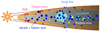Fig. 4 Overview of our models for gas disk and particle evolution in different disk regions. The blue and yellow particles represent silicates with and without refractory carbon. The light blue particles represent icy pebbles. The pink particles show the oxygen atoms that are formed by the destruction of oxygen molecules because of the FUV radiation which is described as red arrows. The light blue dashed line is the snow line. Icy pebbles enclosing many small silicates drift to the snow line (blue dashed line) from the outer region. Orange upper and lower layers are FUV-exposed regions, where oxygen atoms exist.

2.2.5 Size evolution of particles

We used a super-particle approximation. One super-particle represents a huge number of small dust particles. We assigned a single dust size to each super-particle that has the same total mass. We calculated the particle size growth by the “two population model” developed by Birnstiel et al. (2012). The size of the large super-particle is given by $$s(t+\delta t)=\min \left[s_{\max },s(t)\exp \left(Z{\text{Ω}}_{\text{K}}\delta t\right)\right],$$(30)

where $$s_{\max }=\min \left(s_{\text{frag}},s_{\text{drift}}\right),$$(31)

which is the local maximumsize atthe mid-plane corresponding to the Stokes numbers (Eq. (19)) and S_frag and S_drift are the limits by fragmentation and radial drift, given by $${\text{St}}_{\text{frag }}=0.37\frac{v_{\text{frag }}^2}{3\alpha c_s^2}\simeq 2.3\times {10}^{-2}{\left(\frac{v_{\text{frag }}}{10 \text{m}/\text{s}}\right)}^2{\left(\frac{\alpha }{{10}^{-3}}\right)}^{-1}{\left(\frac{T}{150 \text{K}}\right)}^{-1},$$(32) $${\text{St}}_{\text{drift}}=0.40\frac{{\text{Σ}}_{\text{d}}}{{\text{Σ}}_{\text{g}}{C}_{\eta }}{\left(\frac{r{\text{Ω}}_{\text{K}}}{c_s}\right)}^2\simeq 0.49\left(\frac{{\text{Σ}}_{\text{d}}/{\text{Σ}}_{\text{g}}}{{10}^{-3}}\right){\left(\frac{r}{1\text{\hspace{0.17em}au}}\right)}^{-1}{\left(\frac{T}{150 \text{K}}\right)}^{-1}.$$(33)

We set ρ_bulk = 3.0g/cm³ inside the snow line and ρ_bulk = 1.5 g/cm³ outside the snow line.

When s of a super-particle exceeds s_frag, we assume that a collision occurs with υ > υ_frag and randomly chose a new representative particle size by the weight of dN(s) ∝ s^−3.5ds, where N(s) is a cumulative size distribution function, with the maximum and minimum sizes of s_frag and 0.1 µm, conserving the mass of the super-particle. The minimum size is fixed, while s_frag is updated at every timestep.

2.3 Evaporation and recondensation of ice

We consider the evaporation and recondensation of icy particles, following Ciesla & Cuzzi (2006). The decrease rate of the particle mass (m_p) is given by a balance between recondensation and evaporation as (Lichtenegger & Komle 1991) $$\frac{d{m}_{\text{p}}}{dt}=4\pi s^2{v}_{\text{th}}\left({\rho }_{\text{eq}}-{\rho }_{\text{vap }}\right)=2s^2{v}_{\text{th}}^{-1}\left(P_{\text{eq}}-P_{\text{vap }}\right),$$(34)

where ${\rho }_{\text{vap}}={\text{Σ}}_{\text{vap}}/\sqrt{2\pi }{H}_{\text{g}}$ is the vapor density, the averaged normal component of the velocity passing through the particle surface υ_th is given by $$v_{\text{th}}=\frac{c_s}{\sqrt{2\pi }}=\frac{1}{\sqrt{2\pi }}{\left(\frac{k_{\text{B}}T}{{\mu }_{{\text{H}}_2\text{O}}}\right)}^{1/2},$$(35)

with ${\mu }_{{\text{H}}_2\text{O}}$ being the molecular weight of water and we used $$P_{\text{vap }}={\rho }_{\text{vap }}{c}_s^2\text{. }$$(36)

The equilibrium pressure P_eq is given by the Clausius-Clapeyron equation (Lichtenegger & Komle 1991): $$P_{\text{eq}}=1.14\times {10}^{13}\cdot \exp \left(-\frac{6062 \text{K}}{T}\right)\text{g} {\text{cm}}^{-1} {\text{s}}^{-2}.$$(37)

For each super-particle, P_eq and P_vap at the location of the particle are calculated at each timestep. When P_eq > P_vap, the evaporation probability during δt is evaluated as $$p_{\text{evp}}=\min \left(\frac{{\dot{m}}_{\text{p}}\delta t}{m_{\text{p}}},1\right)=\min \left(\frac{2}{v_{\text{th}}}\frac{3}{4\pi {\rho }_{\text{bulk }}s}\left(P_{\text{eq}}-P_{\text{vap }}\right)\delta t,1\right).$$(38)

For a generated random number ℛ in [0,1], if ℛ ≤ p_evp, we regard that the icy super-particle evaporates.

When P_eq < P_vap, recondensation should occur immediately. The change in the water vapor surface density, ∆Σ_vap, should be corresponding to P_vap – P_eq. The recondensation probability is evaluated as $$p_{\text{cnd }}=\min \left(\frac{\text{Δ}{\text{Σ}}_{\text{vap }}}{{\text{Σ}}_{\text{vap }}},1\right)=\min \left(\frac{P_{\text{vap }}-P_{\text{eq }}}{P_{\text{vap }}},1\right).$$(39)

Similarly, the icy super-particle condenses if ℛ ≤ p_cnd for a newly generated ℛ.

We assume water vapor re-condenses on surfaces of both ice and silicate dust particles. Ros et al. (2019) suggested water vapor tends to re-condense on the icy pebbles’ surface rather than the silicate dust surface. Even if we restrict recondensation to silicate particle surfaces, our results hardly change.

In this paper, we define the “snow line” as the radius where the mass fraction of H₂O ice exceeds 1% of total solid mass. In the fiducial case, the snow line radius is r_snow ≃ 3.7 au. We assume that smaller silicate particles are released after an icy particle passes the snow line. Even if fluffy silicate aggregates are first formed as icy mantle evaporates (Aumatell & Wurm 2011), we assume that they are destroyed by collisional fragmentation into grains, for simplicity.

2.4 Carbon destruction rate by FUV

Alata et al. (2014, 2015) suggested that hydrocarbon molecular gas is released from the surface of amorphous hydrocarbons by FUV. They are suggested to exist in the ISM and comets as so-called “amorphous carbons”.

We calculated the carbon fraction change with the carbon depletion timescale: $$\delta f_{\text{c}}=-2\left(\frac{\delta t}{t_{\text{ph}}}+\frac{\delta t}{t_{\text{ox}}}\right)f_{\text{c}},$$(40)

where t_ph and t_ox are timescale of photolysis and oxidation. To suppress a too abrupt change of the carbon fraction, when |δf_c/ f_c| ≥ 0.01 with a dynamical timestep, we adopted a shorter chemical timestep δt_chem, such that |δf_c/f_c| < 0.01. We then recalculated the timescale by updating the particle’s position, assuming that the particle moves linearly during the dynamical timestep δt (Ishizaki et al. 2023). The detailed calculation model is shown in Appendix A.

2.4.1 Opacity for FUV

The vertical optical depth (τ_zλ) for a given wavelength λ is estimated by $${\tau }_{ɀ\lambda }={\kappa }_0{\displaystyle {\int }_{\left|ɀ\right|}^{\infty }{\rho }_{s_{\lambda }}}dɀ,$$(41)

where κ_0λ is the dust opacity for λ. Because the particles with s > s_λ ~ do not contributes to the opacity in the Rayleigh regime, the effective dust density for the opacity, ${\rho }_{s_{\lambda }}$, is given by $${\rho }_{s_{\lambda }}~\frac{{\text{Σ}}_{\text{d}}}{\sqrt{2\pi }{H}_{\text{d}}}\exp \left(-\frac{{ɀ}^2}{2H_{\text{d}}^2}\right)\times {\left(\frac{s_{\lambda }}{s_{\text{max}}}\right)}^{0.5},$$(42)

where H_d is the scale height of dust particles given by $$H_{\text{d}}=\sqrt{\frac{\alpha }{\alpha +\mathrm{St}\left(s_{\lambda },ɀ\right)}}{H}_g,$$(43)

and we used the relation that the mass fraction (ζ) of particles of $s\le s_{\lambda }\text{is}\sim \sqrt{s_{\lambda }/s_{\max }}$ with the assumed size distribution, dN(s) ∝ s^−3.5ds¹. In summary, the vertical optical depth is rewritten as $${\tau }_{ɀ\lambda }={\kappa }_0{\text{Σ}}_{\text{d}}{\left(\frac{s_{\lambda }}{s_{\max }}\right)}^{0.5}\mathrm{erfc}\left(\frac{\left|ɀ\right|}{\sqrt{2}{H}_{\text{d}}}\right).$$(44)

We assumed λ = 0.6 µm and κ₀ ~ 2.5 × 10⁴ cm²g⁻¹, following Binkert & Birnstiel (2023). We also considered the FUV radiation from the central star. Because of the flaring of the disk, the optical depth from the central star is given by τ_r = τ_z/Φ, where Φ is the flaring angle set to 0.05 in our calculations. Figure 5 shows the bottom of the FUV-exposed layer (τ_r ~ 1) for the initial condition of each parameter set.

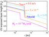Fig. 5 Height of the FUV-exposed layer for the initial condition.

2.4.2 Photolysis rate

The photolysis timescale is estimated by the mean collision time of a photon with a carbon atom of amorphous hydrocarbons (Klarmann et al. 2018; Binkert & Birnstiel 2023): $$t_{\text{ph}}=\frac{4s{\rho }_{\text{c}}}{3Y_{\text{ph}}{F}_{\text{FUV}}{m}_{\text{c}}},$$(45)

where F_FUV is the flax of FUV radiation given by $$F_{\text{FUV}}\text{=}\frac{L_{\text{FUV}}}{4\pi r^2}\text{exp}\left(\text{-}{\tau }_r\right).$$(46)

Here, Y_ph is the yield of photolysis per incoming photon, and m_c and ρ_c is the atomic mass and the bulk density of carbons. We set the yield Y_ph = 10⁻⁴. As Binkert & Birnstiel (2023) suggested photons that penetrate the lower layer could destroy more amorphous hydrocarbons because more particles exist in the lower layer. However, this effect could lower the height of photolysis occurring region only by ≲0.5 H_g (see also Fig.3 in Binkert & Birnstiel 2023).

2.4.3 Oxidation rate

We assume that oxidation occurs only in the exposed layer (τ_r ≤ 1), since Lee et al. (2010) showed that oxygen atoms are abundant in the FUV-exposed layer and the abundance decreased steeply with the decrease of the height. We calculate the timescale of oxidation described by $$t_{\text{OX}}=\frac{4s{\rho }_{\text{c}}}{3n_{\text{OX}}{v}_{\text{OX}}{Y}_{\text{OX}}{m}_{\text{c}}},$$(47)

where υ_ox is the mean thermal velocity of oxygen atoms given by $v_{\text{ox}}=\sqrt{(8/\pi )\left(k_{\text{B}}{T}_{\text{FUV}}/m_{\text{ox}}\right)}$, m_ox is the oxygen atom mass, and Y_ox is the number of carbon atoms removed by an oxygen atom given by (Draine 1979) $$Y_{\text{OX}}=A\exp \left(-\frac{B}{T_{\text{FUV}}}\right),$$(48)

with A = 2.3, B = 2580 K for T_FUV < 440 K and A = 170, B = 4430 K for T_FUV > 440 K. We estimated the number density of oxygen atoms $n_{\text{ox}}=ϵn_{{\text{H}}_2}$, where $n_{{\text{H}}_2}$ is the number density of H₂ given by $$n_{{\text{H}}_2}=\frac{{\text{Σ}}_{\text{g}}}{\sqrt{2\pi }\text{μ}{m}_{\text{p}}{H}_{\text{g}}}\exp \left(-\frac{{ɀ}^2}{2H_{\text{g}}^2}\right).$$(49)

We assumed ϵ = 10⁻⁴, following Klarmann et al. (2018).

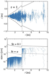Fig. 6 Typical trajectory of a solid particle (upper panel) and the size evolution (lower panel) in a disk with the fiducial parameters. The gray dash-dotted line represents the snow line at rsnow ≃ 3.7 au. The black dotted line of the top panel shows the height of the FUV-exposed layer. The black dotted and dotted lines show the particle sizes corresponding to St = 0.1 and St = α, respectively.

3 Results

3.1 Detailed evolution in the fiducial run

In this section, we show the result of the fiducial run with the disk parameters and the fragmentation velocities in Table 2, assuming that all the refractory carbons are amorphous hydrocarbons

Figure 6 shows a typical trajectory in the z-r and s-r planes of a super-particle which starts at r ≃ 9 au with s = 0.1 µm. In the early phase, growth dominates over drift. In this run, the particle is mostly in a viscously heated region, except for the initial stage (Eq. (8)). Substituting the disk temperature given by Eq. (7) into Eq. (32), the fragmentation-limited Stokes number is St_frag ≃ 0.059 (r/9 au)^3/7. When the particle’s St value exceeds St_frag, we randomly re-assign its size (<s_frag) to a weight corresponding to the given power law. The particle grows up to the size corresponding to St ~ 0.06 around 9 au. After the particle passes the snow line at r_snow ≃ 3.7 au, smaller particles are released to be strongly coupled to the gas (St < α) as a result of the evaporation of icy mantle of the pebbles. Finally, the particle is lifted up inside r_snow.

Figure 7 shows the snapshots of size and vertical distributions of the particles. The colors of particles show the carbon fraction of each particle. The dark navy dots indicate the silicate super-particles that preserve original carbon fraction similar to the solar value (f_c ~ 0.25). The yellow dots inside the snow line represent the silicate super-particles with significantly depleted carbon fraction (f_c ≲ 0.01). The green ones are in between. The size of particles is dramatically changed at the snow line (~3.7 au) due to the difference in stickiness between icy (υ_frag = 10 m/s) and silicate (υ_frag = 1 m/s) particles, as shown in Eq. (32). The mass averaged size of particles is ~s_max/3, where s_max is the maximum dust size (Eq. (31)). The particle size is usually limited by fragmentation rather than drift. The upper panel in Fig. 7a shows that most of the icy pebbles grow up to the size given by s_max (Eq. (31)).

For the icy pebbles, St > α, and their motions are not strongly coupled to the gas, while the motions of the released silicate are strongly coupled (St < α), and the vertical distribution is expanded up to |z|/r ~ 0.1. As a result, the aspect ratio of the icy pebble distribution is considerably lower than that of the small silicate particles (the upper panel in Fig. 7a), and icy pebbles beyond the snow line are usually shielded from FUV from the host star.

Because the contrasts in υ_frag and St/α between inside and beyond r_snow lead to the significant depletion of solid carbon inside rsnow, we explain the growth, drift, and diffusion of particles together with the evolution of f_c in details. The evolution of the radial distribution of the particles is divided into four stages and the carbon fraction is changed according to the stages.

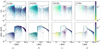Fig. 7 Snapshots of solid super-particles in the r-(|z|/r) plane and size distribution. The upper panels show the snapshots of silicates at (a) 0.2 Myr (~tpf), (b) 0.45 Myr (~tpf + tdrift,ice), (c) 0.92 Myr(~tpf + tdrift,ice + tdiff,snow), and (d) 2.0 Myr. The color bar shows the carbon fraction of each silicate super-particle. The cyan dots show the icy super-particles. The black dashed line shows the height of τFUV = 1. The lower panels show the size distributions of silicates corresponding to the upper panels. The black dashed line shows the local maximum dust size (smax) (Eq. (31)).

3.1.1 Quasi-steady dust accretion stage

The theoretical estimate for pebble formation timescale due to pairwise coagulation in the Epstein regime is (Sato et al. 2016; Ida et al. 2019) $$t_{\text{pf}}~2\times {10}^5{\left(\frac{Z_0}{0.01}\right)}^{-1}{\left(\frac{r}{100\text{\hspace{0.17em}au}}\right)}^{3/2}\text{ years, }$$(50)

where Z₀ is the initial solid-to-gas ratio in the disk. Thus, pebble formation proceeds in an inside-out manner. At t ~ 0. 2 Myr, the pebbles at r ≲ 100 au have already started drifting and the quasi-steady accretion of solids with the silicate particle pile-up inside the snow line has been established.

Because the mean radial velocity of the silicate particles is lower than that of the icy pebbles, the silicate particles released by sublimation of the icy mantle of the pebbles pile up inside the snow line (see the line at t = 0.2 Myr in the top panel of Fig. 8). Since the solid mass flux should be continuous at the snow line, the ratio of solid surface densities from just inside the snow line ∑_d,in to just outside ∑_d,out is given by $$\frac{{\text{Σ}}_{\text{d},\text{ in }}}{{\text{Σ}}_{\text{d},\text{ out }}}=\frac{0.5{\dot{M}}_{\text{d}}}{2\pi r{v}_{r,\text{ in }}}\frac{2\pi r{v}_{r,\text{ out }}}{{\dot{M}}_{\text{d}}}=0.5\frac{v_{r,\text{ out }}}{v_{r,\text{ in }}},$$(51)

where we assume half of the solid mass is converted to the water vapor inside the snow line. Equation (20) is rewritten as $$v_r\simeq -\frac{\text{Λ}}{1+{\text{Λ}}^2{\text{St}}^2}\left(2\text{Λ}\mathrm{St}{C}_{\eta }+\frac{3}{2}\alpha \right)h_{\text{g}}^{2}r\text{Ω}.$$(52)

Inside the snow line, since the released silicate particles are small enough to be coupled with the gas (St ≪ α), their radial velocity is $$v_{r,\text{ in }}\simeq -\frac{3\text{Λ}}{2}\alpha h_{\text{g}}^{2}r\text{Ω}.$$(53)

Outside the snow line, St ≫ α for icy pebbles and the radial drift velocity is given by $$v_{r,\text{ out }}\simeq -2{\text{Λ}}^2\mathrm{St}{C}_{\eta }{h}_{\text{g}}^{2}r\text{Ω}.$$(54)

With Λ ≃ 1, we obtain $$\frac{{\text{Σ}}_{\text{d},\text{in }}}{{\text{Σ}}_{\text{d},\text{ out }}}\simeq 0.5\times \frac{4C_{\eta }{\text{St}}_{\text{frag }}}{3\times 3\alpha }\simeq 6{\left(\frac{\alpha }{{10}^{-3}}\right)}^{-2}{\left(\frac{v_{\text{frag, ice }}}{10 \text{m}/\text{s}}\right)}^2{\left(\frac{T(r_{\text{snow }}}{170 \text{K}}\right)}^{-1},$$(55)

where we substitute Eq. (32) into St ~ St_frag/3 (taking the size distribution into account) and use C_η = 11/8. The numerical result at t = 0.2 Myr in the top panel of Fig. 8 shows that the jump in ∑_d is consistent with the Eq. (55).

The released silicate particles are occasionally stirred up highly by the disk gas turbulence because St ≪α, while they radially go back and forth. As a result, some fraction of amorphous hydrocarbons in these particles are destructed by photolysis and oxidation.

However, f_c decreases only slightly at t = 0.2 Myr (lower panel of Fig. 8) because fresh silicate particles full of amorphous hydrocarbons are steadily supplied and well mixed with particles where the amorphous hydrocarbons become destructed. This is consistent with the result found by Klarmann et al. (2018).

To highlight the effect of the continuous supply, we carried out a hypothetical case where all the radial motion is set to zero. Because the pebble flux is also stopped, the fresh refractory car-bon supply is also stopped. The carbon fraction changes only through vertical diffusion, photolysis, and oxidation. As shown by the black line in Fig. 9, this process efficiently depletes f_c on a timescale of 50 kyr.

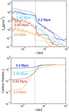Fig. 8 Time evolution of the solid surface density ∑d (upper panel) and the carbon fraction, fc, (lower panel) of the fiducial run. The gray dash-dotted line shows the snow line. The dotted lines in the upper panel show the analytical estimations given by Eq. (68). The dash-dotted lines represent the snow line at rsnow ~ 3.7 au.

3.1.2 Icy pebble flux decaying stage

However, the quasi-steady accretion ends, and the carbon deple-tion pattern changes, when the pebble formation front reaches the disk’s outer edge at the characteristic radius r_disk. Then, because most of the reservoir of solid materials is consumed, the pebble flux rapidly decays (Sato et al. 2016; Ida et al. 2019).

The duration of the quasi-steady supply of icy pebbles is given by t_pf(r_đısk) + t_drift,ice, where t_drift,ice is the drift timescale from the disk outer edge to the snow line. The drift velocity is given by $$\begin{array}{l}{v}_r\simeq 2{\text{Λ}}^2\mathrm{St}{C}_{\eta }{h}_{\text{g}}^{2}r\text{Ω}\\ \simeq 7.8\times {10}^{-5}{\text{Λ}}^2{\left(\frac{\alpha }{{10}^{-3}}\right)}^{-1}{\left(\frac{v_{\text{frag }}}{10 \text{m}/\text{s}}\right)}^2{\left(\frac{r}{1\text{au}}\right)}^{1/2}\text{au}/\text{y}.\end{array}$$(56)

Because $h_{\text{g}}^2\propto T$, the T-dependence is canceled out with T⁻¹ in St ≃ St_frag/3. The α-dependence appears from St ∝ 1/α in the fragmentation limit. The factor Λ = (1 + ρ_d/ρ_g)⁻¹ is estimated by $$\frac{{\rho }_{\text{d}}}{{\rho }_{\text{g}}}=\frac{{\text{Σ}}_{\text{d}}}{{\text{Σ}}_{\text{g}}}\frac{H_{\text{g}}}{H_{\text{d}}}\sim \frac{{\text{Σ}}_{\text{d}}}{{\text{Σ}}_{\text{g}}}\sqrt{\frac{\text{St}}{\alpha }}$$(57) $$\simeq 0.13\left(\frac{{\text{Σ}}_{\text{d}}/{\text{Σ}}_{\text{g}}}{0.01}\right){\left(\frac{\alpha }{{10}^{-3}}\right)}^{-1}\left(\frac{v_{\text{frag}}}{10\text{m}/\text{s}}\right){\left(\frac{r}{100\text{\hspace{0.17em}au}}\right)}^{3/14}.$$(58)

Here, we use Eq. (43) for H_d assuming St ≫ α and the irradiation-dominated T distribution is applied in the regions outside the snow line (Eq. (7)). Then, t_drift,ice is estimated as $$\begin{array}{l}{t}_{\text{drift,ice }}=-\underset{r_{\text{snow }}}{\overset{r_{\text{disk }}}{{\displaystyle \int }}}\frac{dr}{v_r}~3.1\times {10}^5\left(\frac{\alpha }{{10}^{-3}}\right){\left(\frac{10 \text{m}/\text{s}}{v_{\text{frag },ice}}\right)}^{-2}\hfill \\ \times {\left(\frac{1+{\rho }_{\text{d}}/{\rho }_{\text{g}}}{1.1}\right)}^2\left(\sqrt{\frac{r_{\text{disk }}}{100\text{\hspace{0.17em}au}}}-0.1\sqrt{\frac{r_{\text{snow }}}{1\text{\hspace{0.17em}au}}}\right)\text{ years}.\hfill \end{array}$$(59)

In the fiducial run, t_drift,ice is estimated to be about 2.5 × 10⁵ years.

The second stage starts at t ~ t_pf + t_drift,ice (~0.45 Myr in the fiducial run). In this stage, while ∑_d inside the snow line has not been reduced, the carbon fraction f_c starts decreasing. Figure 7b shows the vertical and size distributions at t = 0.45 Myr. The total mass of dust particles inside r_snow is larger than that out-side it, since most of the icy pebbles carrying silicate particles had drifted to the regions inside r_snow. The upper panel of Fig. 8 shows the evolution of ∑_d. The ∑_d beyond r_snow significantly drops from the first phase (t = 0.2 Myr) to the second phase (t = 0.45 Myr), while the ∑_d decay is not significant inside r_snow. As a result, ∑_d jumps at r_snow by as much as a factor of 30. How-ever, carbon depletion proceeds only by a factor of a few from the first to the second stage, because supply of icy pebbles still remains at a reduced rate.

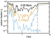Fig. 9 Time evolution of carbon fraction, fc, when the particles diffuse only vertically and neither drift nor diffuse radially.

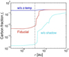Fig. 10 Carbon fraction, fc, at 0.68 Myr in the fiducial run, without the vertical temperature profile, and without the shadow area outside the snow line.

3.1.3 Silicate dust surface density decaying stage

In the third stage, ∑_d decreases also inside r_snow. Because the influx of silicate particles from the outer region is already diminished, the decrease occurs on a diffusion timescale at r_snow (Okamoto & Ida 2022): $$\begin{array}{l}{t}_{\text{diff, snow }}{~\frac{r^2}{\alpha H_{\text{g}}^2{\text{Ω}}_{\text{K}}}|}_{r_{\text{snow }}}={\frac{1}{\alpha h_{\text{g}}^2{\text{Ω}}_{\text{K}}}|}_{r_{\text{snow }}}\\ ~4.7\times {10}^5{\left(\frac{\alpha }{{10}^{-3}}\right)}^{-10/9}{\left(\frac{{\dot{M}}_{\text{g}}}{{10}^{-8}{M}_{\odot }{\text{yr}}^{-1}}\right)}^{2/9}\text{ years}.\end{array}$$(60)

In the fiducial run, t ~ t_pf + t_drift,ice + t_drift,snow ~ 0.92 Myr. The upper panel of Fig. 8 shows that at t = 0.92 Myr, ∑_d inside r_snow is decreased by a factor of several from that at t = 0.45 Myr.

In this stage, f_c shows a pronounced hyperbolic-tangent-function-like (tanh-like) depletion pattern near the snow line by more than one order of magnitude (the line of t = 0.92 Myr). The greater depletion is due to the diminished influx of silicate particles from the outer region. The flat f_c pattern at ≲1 au is caused by higher ∑_d there. Because photolysis is inefficient there, f_c conserves that in the outer region.

The pronounced decrease in f_c around r_snow is not originated mainly by the shadow effect, that amorphous hydrocarbons are not destroyed outside r_snow due to the FUV shielding that we adopt (Sect. 2.2.2). In Fig. 10, the fiducial case result is compared with the result without the shadow effect at 0.68 Myr(~t_pf + t_drift,ice+ 0.5 t_drift,snow), where the similar drop-off in f_c around r_snow is shown. While f_c is decreased at r ≳ r_snow, the non-shadow effect just lowers the baseline of f_c in the inner region.

We have argued that the tanh-like f_c pattern is formed by a jump in ∑_d across r_snow. After 0.92 Myr, since ∑_d is depleted also inside r_snow, it could be predicted that f_c goes up again. However, Fig. 8 shows that f_c further decreases while the enhanced jump in ∑_d at ~r_snow disappears. This is caused by more efficient photolysis, associated with the opacity decrease due to the ∑_d decay, which overwhelms the effect of the reduced jump of ∑_d at ~r_snow. As this effect also narrows the area where f_c is flat, the tanh-like f_c pattern is diminished.

3.2 Analytical formula for ∑_d across the snow line

We found that the carbon fraction inside the snow line is reg-ulated by the ratio of ∑_d inside and outside the snow line, except for the final phase with highly depleted ∑_d. To explain the numerical results, we analytically estimate the ∑_d distribution. The solid-to-gas ratio with Λ≪1 is given by (Eq. (53)): $$Z=\frac{{\text{Σ}}_{\text{d}}}{{\text{Σ}}_{\text{g}}}=\frac{2\pi r\left|u_v\right|}{2\pi r\left|v_r\right|}\frac{{\dot{M}}_{\text{d}}}{{\dot{M}}_{\text{g}}}\simeq \frac{3\alpha h_{\text{g}}^2/2}{h_{\text{g}}^2\left(2C_{\eta }\text{St}+3\alpha /2\right)}\frac{{\dot{M}}_{\text{d}}}{{\dot{M}}_{\text{g}}}.$$(61)

In a steady accretion disk region, Ṁ_d/Ṁ_g is constant with r. When St ≪ α, corresponding to the region at r < r_snow, $$Z\simeq {\dot{M}}_{\text{d}}/{\dot{M}}_{\text{g}}.$$(62)

On the other hand, for St ≪ α at r > r_snow, Z ∝ St⁻¹. As Eqs. (32) and (33) show, the drift limit is more stringent at rel-atively large r, where the dust density is lower and collisions are less frequent. For r > r_dri–fra (the transition radius between the drift and fragmentation limits), St ~ St_drift/3 ∝ ZT⁻¹r⁻¹ (Eq. (33). Deleting St from this relation and Z ∝ St⁻¹, we obtain $$Z(r)\simeq Z\left(r_{\text{disk }}\right){\left(\frac{T(r)}{T\left(r_{\text{disk }}\right)}\right)}^{1/2}{\left(\frac{r}{r_{\text{disk }}}\right)}^{1/2},$$(63)

where r_disk is the disk radius. In the outer disk region (r > r_vis–irr), irradiation is dominant and T ∝ r^−3/7. Thus, $$Z=\frac{{\text{Σ}}_{\text{d}}}{{\text{Σ}}_{\text{g}}}\simeq Z\left(r_{\text{disk }}\right)\cdot {\left(\frac{r}{r_{\text{disk }}}\right)}^{2/7}.$$(64)

Substituting this equation into Eq. (33), we obtain $${\text{St}}_{\text{drift }}=0.13\left(\frac{Z\left(r_{\text{disk }}\right)}{{10}^{-3}}\right){\left(\frac{r}{1\text{\hspace{0.17em}au}}\right)}^{-5/7}{\left(\frac{r_{\text{disk }}}{100\text{\hspace{0.17em}au}}\right)}^{-2/7}{\left(\frac{T}{150 \text{K}}\right)}^{-1}.$$(65)

Comparing this with Eq. (32), the transition radius r_dri–fra is given by $$r_{\text{dri-fra }}=11{\left(\frac{Z\left(r_{\text{disk }}\right)}{{10}^{-3}}\right)}^{7/5}{\left(\frac{r_{\text{disk }}}{100\text{\hspace{0.17em}au}}\right)}^{-2/5}{\left(\frac{v_{\text{frag }}}{10 \text{m}/\text{s}}\right)}^{-14/5}{\left(\frac{\alpha }{{10}^{-3}}\right)}^{7/5}\text{ au}.$$(66)

For r < r_dri–fra, Z ∝ St⁻¹ with Eq. (32) shows $$Z(r)\simeq Z\left(r_{\text{dri-fra }}\right)\left(\frac{T(r)}{T\left(r_{\text{dri}-\text{fra}}\right)}\right).$$(67)

Inside the snow line, Z is constant with r (Eq. (62)). Because ∑_g ∝ r^−1/2 in this region (Eqs. (1) and (6)), ∑_d ∝ r^−1/2. The ratio of ∑_d just inside the snow line to just outside it is given by Eq. (55). Thus, in the steady accretion disk regions, $$Z(r)=\{\begin{array}{ll}Z\left(r_{\text{disk }}\right){\left(\frac{r}{r_{\text{disk }}}\right)}^{2/7}\hfill & \left[r>r_{\text{dri-fra }}\right]\hfill \\ Z\left(r_{\text{dri-fra }}\right)\left(\frac{T(r)}{T\left(r_{\text{dri-fra }}\right)}\right)\hfill & \left[r_{\text{snow }}<r<r_{\text{dri-fra }}\right]\hfill \\ Z\left(r_{\text{snow }}\right)\times 6{\left(\frac{\alpha }{{10}^{-3}}\right)}^{-2}{\left(\frac{v_{\text{frag,ice }}}{10 \text{m}/\text{s}}\right)}^2\hfill & \hfill \\ \times {\left(\frac{T\left(r_{\text{snow }}\right)}{170 \text{K}}\right)}^{-1}{\left(\frac{r}{r_{\text{snow }}}\right)}^{-1/2}\hfill & \left[r<r_{\text{snow }}\right].\hfill \end{array}$$(68)

Here, Z(r_dri–fra) = Z(r_disk)(r_dri–fra/r_disk)^2/7 and Z(r_snow) = Z(r_dri–fra)(T(r_snow)/T(r_dri–fra)). The steady accretion across the snow line would continue until ∑_d inside the snow line starts to decay (t ~ t_pf + t_drift,snow ~ 0.45 Myr).

Equation (68) shows that once Z(r_disk) is given, the ∑_d distribution is estimated (∑_d = Z ∑_g; ∑_g is given by the simulation parameter Ṁ_g). Before the pebble formation front arrives at r_disk, Z(r_disk) is given by its initial value Z₀ ~ 0.01. After that, Z(r_disk) is rapidly reduced. Ida et al. (2019) derived the time evolution of Z(r_disk) as $$Z\left(r_{\text{disk }}\right)~Z_0{\left(1+t/t_{\text{pf}}\right)}^{-\gamma },$$(69)

where $$\gamma ~1+0.15\left(300\text{\hspace{0.17em}au}/r_{\text{disk }}\right).$$(70)

The dashed lines in the upper panel of Fig. 8 show the analytical estimate of ∑_d given by substituting Eq. (69) into Eq. (68). The ∑_d distribution at ≳r_snow is well fitted by the analytical estimate for all of the four different times (0.2–1.5 Myr). At t = 0.45 and 0.92 Myr, it is fitted also in the region inside the snow line except for the innermost region. For this duration, ∑_d is also decaying and the steady accretion is established.

3.3 Important parameters for carbon depletion

3.3.1 The v_frag change across the snow line

Detailed descriptions of the evolution of particles in Sect. 3.1 strongly suggest that the conditions for the tanh-like pattern of ƒ_c are an enhanced jump in ∑_d at ~r_snow and early decay of icy pebble flux that reduces the supply of fresh amorphous hydrocarbons to the region inside r_snow. The both features are originated from v_frag,sil < v_frag,ice such that St ~ α at r < r_snow and St ≫ α at r > r_snow.

The decay of icy pebble flux starts at t ~ t_pf + t_drift,ice where t_pf and t_drift,ice are given by Eqs. (50) and (59). For Z₀ = 0.01 and r_snow = 3.7 au, we have $$t_{\text{pf}}~2\times {10}^5{\left(\frac{r_{\text{disk }}}{100\text{\hspace{0.17em}au}}\right)}^{3/2}\text{ years, }$$(71) $$t_{\text{drift },\text{ ice }}~2.5\times {10}^5\left(\frac{\alpha }{{10}^{-3}}\right){\left(\frac{10 \text{m}/\text{s}}{v_{\text{frag },i\text{ce}}}\right)}^{-2}{\left(\frac{r_{\text{disk }}}{100\text{\hspace{0.17em}au}}\right)}^{1/2}\text{ years}.$$(72)

The drift timescale is shorter for larger v_frag,ice. For the early decay of the supply of fresh amorphous hydrocarbons to occur, t_drift,icemust be short enough compared with global disk gas depletion timescale t_disk ~ 3 × 10⁶(α/10⁻³)⁻¹(r_disk/100au) yr, which is equivalent to $$v_{\text{frag,ice }}\gtrsim 3.2\left(\frac{\alpha }{{10}^{-3}}\right){\left(\frac{r_{\text{disk }}}{100\text{\hspace{0.17em}au}}\right)}^{-1/4} \text{m}/\text{s}.$$(73)

Here, we confirm the above conditions by performing the runs with different combinations of v_frag,ice and v_frag,sil. Figure 11 shows ∑_d and ƒ_c at 0.68 Myr for v_frag,icee = v_frag,sil = 10m/s (the blue line), v_frag,icee = v_frag,sil = 1 m/s (the cyan line), and the fidu-cial case (the red line) at 0.68 Myr, which is the intermediate time of the third stage (~t_pf + t_drift,ice + 0.5t_diff,snow). To highlight the v_frag effect, the shadow effect is applied even in the case of v_frag,icee = v_frag,sil. The results without the shadow effect are shown in Appendix B.

In the run with v_frag,icee = v_frag,sil = 1 m/s, for both silicate par-ticles and ice pebbles, St = 2.1 × 10⁻⁴ at the snow line. Because St < α, silicate particles do not accumulate inside the snow line and ƒ_c decreases only slightly inside r_snow.

When v_frag,icee = v_frag,sil = 10 m/s, for both silicate particles and ice pebbles, St = 2.1 × 10⁻² at the snow line, and particles are also not piled up except around the snow line. Since the pile-up around the snow line is caused by recondensation of water vapor diffusing out from inside the snow line, it does not sig-nificantly influence the motions of the silicate particles, and ƒ_c decreases only slightly as well.

On the other hand, when v_frag,ice = 10m/s and v_frag,sil = 1 m/s, St = 2.1 × 10⁻⁴ < α for silicate particles and St = 2.1 × 10⁻² > α. Accordingly, the pile-up occurs and ƒ_c significantly decreases with the tanh-like shape.

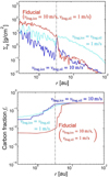Fig. 11 Distributions of ∑d and ƒc at 0.68 Myr for vfrag,icee = vfrag,sil = 1 m/s and 10 m/s and the fiducial case (vfrag,icee = 10m/s and vfrag,sil = 1 m/s).

3.3.2 The vertical temperature profile

The upper panel of Fig. 12 shows ƒ_c at 0.1 Myr with and without vertical temperature profile (see Fig. 3). To highlight this effect, we stop the radial motion of particles. The carbon fraction ƒ_c is the minimum at r ~ 1 −2 au. The lower panel shows the ratio of vertical diffusion timescale in the FUV-exposed layer to that at the mid-plane. The ratio is the smallest at r ~ 2 au inside r_snow. Because the temperature is significantly higher in the upper layer than around the mid-plane at ~1 au, the diffusion there leads to more photodegradation of amorphous hydrocarbons. The car-bon fraction outside the snow line (~3.7 au) does not decrease because the icy pebbles are not particularly stirred up. While the radial drift is neglected in Fig. 12, a significant impact of the vertical temperature profile on the carbon depletion is also shown in Fig. 10, where the radial drift is included.

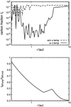Fig. 12 Carbon fraction at 0.1 Myr with and without vertical temperature profile (upper panel) and ratio of vertical diffusion timescale at FUV-exposed layer to mid-plane (lower panel). In these runs, the radial drift is neglected to highlight the effect of the vertical temperature profile.

3.3.3 Other parameter dependencies

We also carried out runs with a different value for each parameter from the fiducial run, α = 5 × 10⁻⁴, υ_frag,sil = 0.1 m/s, and Z₀ = 0.05. In these cases, St ≲ α inside r_snow and St ≫ α outside it, which is equivalent to the two conditions of the pile-up of silicate particles and earlier decay of icy pebble flux are satisfied. In these cases, the tanh-like shaped f_c pattern is produced with small variations in the bottom values (Fig. 13), as expected. The detail results are shown in Appendix C.

The only exception is the case with Ṁ_g = 10⁻⁹ M_⊙/yr, where the disk opacity is significantly lower. As the silicate particles drift to inner regions, the carbon destruction proceeds to result in qualitatively different f_c shape.

4 Discussion

4.1 Pyrolysis of complex organics

So far we have not included complex organics, because it is likely that some fraction of the products of their pyrolysis are amorphous hydrocarbons (Sect. 1). In Fig. 14, we show the result with initial solid carbon of a mixture of complex organics with T_des = 540 K (50 wt.%) and amorphous hydrocarbons (50 wt.%). The simulation parameters are the same as the fiducial case. The pyrolysis of complex organics occurs even near the disk mid-plane. In the runs in Fig. 14, however, we still assume that half the mass of the complex organics is converted into amorphous hydrocarbons through this reaction. Even though at 0.92 Myr, the total carbon fraction f_c inside the pyrolysis line shows a slightly lower value than outside of it, the difference is not significant enough to explain the discrepancy between chondrites and the bulk Earth.

The initial ratio of complex organics and amorphous hydrocarbons and the conversion rate of complex organics to amorphous hydrocarbons through pyrolysis remain unclear. Adjusting these values could allow the f_c pattern to better reproduce the lower f_c observed in the bulk Earth compared to chondrites.

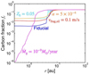Fig. 13 Carbon fraction at 0.68 Myr for different parameter sets.

4.2 FUV radiation outside the snow line

We assumed carbon destruction does not occur outside the snow line because FUV radiation from the host star is hindered by piled-up dust inside the snow line. However, the “shadow area” may only extend up to ~10 au (Ohno & Ueda 2021).

However, this could not be effective enough to erase the dichotomy in f_c between the inner and outer disk regions. As shown in Fig. 10, the f_c distribution shows the tanh-like pattern also in the case without the shadow area. This result suggests that the limited shadow region and the interstellar FUV radiation do not break the higher carbon fraction at the outer disk region than the inner disk region. However, as discussed in Sect 4.5, the result without the shadow area may be inconsistent with the observation of the comets.

4.3 Oxidation

We assumed amorphous hydrocarbon is oxidized only if the dust exists in the FUV-exposed layer (τ ≲ 1). However, a few oxygen atoms might exist in the lower layer (e.g., Lee et al. 2010; Anderson et al. 2017). Therefore, oxidation in the lower layer might reduce the carbon abundance.

Moreover, the carbon particle might be oxidized by OH radicals (e.g., Finocchi et al. 1997; Gail & Trieloff 2017). OH radicals are thought to be formed by thermal dissociation of H₂O at the hotter region (T ≳ 1100 K) (e.g., Gail & Trieloff 2017). The abundance of OH radicals in the inner disk region has some uncertainty as Finocchi et al. (1997) estimated 10⁻¹⁰−10⁻⁷ relative to H₂ and Gail & Trieloff (2017) calculated 10⁻¹²−10⁻⁹ relative to H₂ at T ≳ 1100 K. Although the OH abundance is not expected to be high, oxidation by OH might also reduce more carbon particles (Gail & Trieloff 2017). The calculation with a more accurate estimation of OH radical and oxygen atom abundances is left to a future study.

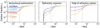Fig. 14 Carbon fraction, fc, with a mixture of complex organics with Tdes = 540 K (50 wt.%) and amorphous hydrocarbons (50 wt.%). The left figure shows the mass fraction of amorphous hydrocarbons, the middle panel shows that of complex organics, and the right panel shows the total carbon fraction. The gray dash-dotted and dotted lines snow the snow and pyrolysis lines.

4.4 Other processes: Gap or pressure bump in the gas disk

Klarmann et al. (2018) concluded that carbon depletion needs some mechanisms that stop the inward solid particles’ flux, such as a gap or a pressure bump in the gas disk. However, the significant reduction in the inward solid particles’ flux by the gap or pressure bump should lower Σ_d and the disk optical depth, the flat f_c pattern would not appear (Fig. 13).

Klarmann et al. (2018) calculated the evolution of Σ_d with single-sized particles. The different sizes between icy pebbles and silicate particles released at the snow line cause pile-up of the silicate particles without the gap or pressure bump (Saito & Sirono 2011; Ida & Guillot 2016; Schoonenberg & Ormel 2017; Ida et al. 2021). In this paper, we have shown that this effect can result in significant carbon depletion.

4.5 Comparison to the observational data

It is shown that chondrite meteorites in the matrix scaling universally show f_c ~ 0.01 (Fig. 1 and Alexander et al. 2007). Our simulations show a flat bottom value of the tanh-like shape as f_c ~ 0.02–0.03 inside the snow line, which is consistent with the chondrite data, if their parent bodies were formed inside the snow line (Fig. 15). The further smaller f_c of the bulk Earth could be potentially accounted for by including complex organics as well as amorphous hydrocarbons and some adjustments of their initial abundance ratio and conversion rate from complex organics to amorphous hydrocarbons through pyrolysis (Sect. 4.1). Comets have f_c as high as ISM, which is also consistent with the tanh-like pattern that our calculations produce (see also Sect. 4.2).

As discussed in Sect. 1, the observed f_c on the WD photospheres, which should reflect the bulk compositions of asteroids or rocky planets around the WDs, is distributed from the solar value far down to the bulk Earth value. We found that the conditions to produce the tanh-like depletion pattern of solid carbon are not too severe, but may be sensitive to details of dust particle properties (and possibly to the disk parameters). This may produce a diversity of f_c values in a range of a few orders of magnitude. It could be responsible for the observed large variety of C/Si ratios on the WD photo-spheres. More detailed comparisons are left for future works.

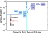Fig. 15 Expect the formation region for each rocky body based on our calculation results.

5 Conclusion

Rocky bodies in the inner Solar System are depleted in carbon compared to the Sun, by one to several orders of magnitude, although most solid carbonaceous components should be refractory in the ISM and the comets. Possible mechanisms to destruct refractory carbonaceous components are photolysis (Alata et al. 2014, 2015) and oxidation for highly refractory carbons such as amorphous hydrocarbons (e.g., Draine 1979) in the upper FUV-exposed layer and pyrolysis for modestly complex organics (e.g., Chyba et al. 1990). However, previous theoretical models (Klarmann et al. 2018; Binkert & Birnstiel 2023) did not succeed in reproducing the observed significant carbon depletion in the case of highly refractory carbons.

We performed a 3D Monte Carlo simulation to track super-particles trajectories in a steady accretion gas disk, taking account of the effects that were not considered in the previous models. We found that the carbon fraction, f_c, is lower by two orders of magnitude inside the snow line when the following conditions are present:

1. The fragmentation limit velocity of silicate particles is lower than that of icy pebbles so that St ≲ α for silicate particles and St ≫ α for icy pebbles;

2. The gas temperature is considerably higher in the upper optically thin layer than near the mid-plane.

The first condition leads to a pile-up of silicate particles inside the snow line and earlier decay of icy pebble flux incoming to the snow line than the depletion of the silicate particles. The latter is shown by globally calculating the growth and radial drift of pebbles in the disk. The second condition leads to more effective vertical diffusion in the upper optically thin layer. Because the FUV-exposed layer is as high as ~4 H_g, the effective vertical diffusion can significantly enhance photolysis.

The matrix-scaled f_C is similar (one to two orders of magnitude depletion) among carbonaceous, ordinary, and enstatite chondrites, while the orbital radii of their parent bodies may be diverse. This feature is well reproduced by our simulations with highly refractory carbon (amorphous hydrocarbons). The bulk Earth could have further lower f_c (three to four orders of magnitude depletion). This feature might also be reproduced if the refractory carbon source is a mixture of amorphous hydrocarbons and (modestly) complex organics.

The first and second conditions are not too severe, but still sensitive and their effects could be responsible for the observed large variety of C/Si on white dwarf photo-spheres, which would be polluted by rocky bodies that existed around the white dwarfs. Theoretical investigations of the carbon deletion problem in the inner Solar System can offer insights into the origin of the large variety of C/Si in rocky bodies in exoplanetary systems. If the f_c values of Earth-size planets in exoplanetary habitable zones have a variation by a few (or more) orders of magnitude, the surface environments (and even interiors) of these planets should exhibit a broad scope of diversity. More studies are needed to explore these issues in depth.

Acknowledgement

We thank the referee for his insightful and encouraging comments. We also thank Shogo Tachibana, Hideko Nomura, and Chris Ormel for helpful discussions. This work was supported by JST Tokyo-Tech SPRING, Grant Number JPMJSP2106, and JSPS Kakenhi 23KJ0885 and 21H04512.

Appendix A Tuning for a higher resolution of smaller particles

Small particles tend to be lifted up to the higher layer more easily. As discussed in Sect. 2.4.1, the mass fraction of particles smaller than 0.1 µm is given by (0.1 µm/s_max)^0.5. If s_max > 1 mm, their mass fraction is less than 1%. We assume the super-particles as aggregations of solid particles with a single size and that all super-particles have equal mass. When the mass fraction of the particles with s ≤ 0.1 µm is less than 1%, the number of super-particles should be higher than 100 to ensure the presence of the small particles. However, as shown in Eq. (28), the typical number of super-particles inside 1 au is less than 100. Thus, the probability of the super-particles with s ≤ 0.1 µm existing inside 1 au is very low.

To adjust the influence of small particles, we add ‘small’ super-particles with a fixed size of 0.1 µm. These are used only for the calculation of f_c, and the Σ_d is calculated by the number of the ‘large’ super-particles alone.

In each timestep, we calculate the mass-averaged carbon fraction between the small and large super-particles given by $$f_{\text{c}}=f_{\text{c}, \text{s}}{\left(\frac{0.1\mu \text{m}}{s_{\max }}\right)}^{0.5}+f_{\text{c},1}\left(1-{\left(\frac{0.1\mu \text{m}}{s_{\max }}\right)}^{0.5}\right),$$(A.1)

where f_c,s and f_c,l are the mass-averaged carbon fractions for small and large super-particles, respectively. We consider the redistribution of carbon between the small and large particles through coagulation andfragmentation ofsolids and assume that all super-particles in each bin have the average carbon fraction in the next timestep.

Appendix B The cases of υ_frag,sil = υ_frag,ice without the shadow area

Fig. B.1 Same as Fig. 11 but without the shadow area behind the snow line.

As argued in Sect. 3.3.1, for υ_frag,sil = υ_frag,ice, the shadow area should not appear behind the snow line. Figure B.1 shows fc at 0.68 Myr without the shadow area. The different fragmentation velocities between icy and silicate particles make a larger dichotomy in f_c between the inner and outer disk region than the other cases even if we do not consider the shadow area. The flat region in the same fragmentation velocity cases might be produced by the inefficiency of photolysis there as shown in Fig. 12.

Appendix C Results with different parameter sets

Figure C.1 shows the time evolution of the solid surface densities (Σ_d) and f_c for different parameter sets. The times of the four lines are corresponding to the four stages discussed in Sect. 3.1. In the lower gas accretion rate stage (final stage), Ṁ_g = 10⁻⁹ M_⊙/year, we stopped the calculation at 1 Myr, when the total solid mass inside the snow line is lower than the Earth’s mass.

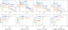Fig. C.1 Time evolution of the solid surface densities (top row) and carbon fractions (bottom row) for each parameter set. The sub-captions show the parameter which we changed from the fiducial parameter set. The dashed lines in the top row show the analytic estimation given by Eq. 68.

References

All Tables

All Figures

Fig. 1 Carbon fraction of Solar System bodies, where the carbon fraction, fc, is defined by the mass fraction of carbon in the sum of solid carbon and the silicates. For ISM dust, comets, and IDPs, this fraction is calculated from the C/Si atomic ratio (Matrajt et al. 2005; Bardyn et al. 2017; Bergin et al. 2015; Binkert & Birnstiel 2023, and references therein). For comparison, we also plot the “Sun” values (fc ≃ 0.25), which refer to hypothetical dust with solar C/Si. The fractions of chondrites are normalized by the matrix volume of each chondrite (see the main text). While Bergin et al. (2015) and Binkert & Birnstiel (2023) showed fc fraction monotonically decreases as the decrease in the heliocentric radius decreases, the matrix-normalized fc of chondrites may be independent of the distance. The uncertainties of chondrites’ fc values come from the variation among each chondrite. The very low fc of BSE and “bulk Earth” are also discussed in the main text.

In the text

	Fig. 2 Gas surface density, Σg, (upper panel) and the mid-plane temperature (lower panel) in the fiducial run.
In the text

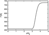	Fig. 3 Vertical temperature profile at 1 au given by Eq. (10).
In the text

Fig. 4 Overview of our models for gas disk and particle evolution in different disk regions. The blue and yellow particles represent silicates with and without refractory carbon. The light blue particles represent icy pebbles. The pink particles show the oxygen atoms that are formed by the destruction of oxygen molecules because of the FUV radiation which is described as red arrows. The light blue dashed line is the snow line. Icy pebbles enclosing many small silicates drift to the snow line (blue dashed line) from the outer region. Orange upper and lower layers are FUV-exposed regions, where oxygen atoms exist.

In the text

	Fig. 5 Height of the FUV-exposed layer for the initial condition.
In the text

	Fig. 6 Typical trajectory of a solid particle (upper panel) and the size evolution (lower panel) in a disk with the fiducial parameters. The gray dash-dotted line represents the snow line at rsnow ≃ 3.7 au. The black dotted line of the top panel shows the height of the FUV-exposed layer. The black dotted and dotted lines show the particle sizes corresponding to St = 0.1 and St = α, respectively.
In the text

Fig. 7 Snapshots of solid super-particles in the r-(|z|/r) plane and size distribution. The upper panels show the snapshots of silicates at (a) 0.2 Myr (~tpf), (b) 0.45 Myr (~tpf + tdrift,ice), (c) 0.92 Myr(~tpf + tdrift,ice + tdiff,snow), and (d) 2.0 Myr. The color bar shows the carbon fraction of each silicate super-particle. The cyan dots show the icy super-particles. The black dashed line shows the height of τFUV = 1. The lower panels show the size distributions of silicates corresponding to the upper panels. The black dashed line shows the local maximum dust size (smax) (Eq. (31)).

In the text

	Fig. 8 Time evolution of the solid surface density ∑d (upper panel) and the carbon fraction, fc, (lower panel) of the fiducial run. The gray dash-dotted line shows the snow line. The dotted lines in the upper panel show the analytical estimations given by Eq. (68). The dash-dotted lines represent the snow line at rsnow ~ 3.7 au.
In the text

	Fig. 9 Time evolution of carbon fraction, fc, when the particles diffuse only vertically and neither drift nor diffuse radially.
In the text

	Fig. 10 Carbon fraction, fc, at 0.68 Myr in the fiducial run, without the vertical temperature profile, and without the shadow area outside the snow line.
In the text

	Fig. 11 Distributions of ∑d and ƒc at 0.68 Myr for vfrag,icee = vfrag,sil = 1 m/s and 10 m/s and the fiducial case (vfrag,icee = 10m/s and vfrag,sil = 1 m/s).
In the text

	Fig. 12 Carbon fraction at 0.1 Myr with and without vertical temperature profile (upper panel) and ratio of vertical diffusion timescale at FUV-exposed layer to mid-plane (lower panel). In these runs, the radial drift is neglected to highlight the effect of the vertical temperature profile.
In the text

	Fig. 13 Carbon fraction at 0.68 Myr for different parameter sets.
In the text

	Fig. 14 Carbon fraction, fc, with a mixture of complex organics with Tdes = 540 K (50 wt.%) and amorphous hydrocarbons (50 wt.%). The left figure shows the mass fraction of amorphous hydrocarbons, the middle panel shows that of complex organics, and the right panel shows the total carbon fraction. The gray dash-dotted and dotted lines snow the snow and pyrolysis lines.
In the text

	Fig. 15 Expect the formation region for each rocky body based on our calculation results.
In the text

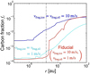	Fig. B.1 Same as Fig. 11 but without the shadow area behind the snow line.
In the text

	Fig. C.1 Time evolution of the solid surface densities (top row) and carbon fractions (bottom row) for each parameter set. The sub-captions show the parameter which we changed from the fiducial parameter set. The dashed lines in the top row show the analytic estimation given by Eq. 68.
In the text

References

- Alata, I., Cruz-Diaz, G. A., Muñoz Caro, G. M., & Dartois, E. 2014, A&A, 569, A119 [NASA ADS] [CrossRef] [EDP Sciences] [Google Scholar]
- Alata, I., Jallat, A., Gavilan, L., et al. 2015, A&A, 584, A123 [NASA ADS] [CrossRef] [EDP Sciences] [Google Scholar]
- Alexander, C. M. O. D., Fogel, M., Yabuta, H., & Cody, G. D. 2007, Geochim. Cosmochim. Acta, 71, 4380 [NASA ADS] [CrossRef] [Google Scholar]
- Anderson, D. E., Bergin, E. A., Blake, G. A., et al. 2017, ApJ, 845, 13 [NASA ADS] [CrossRef] [Google Scholar]
- Aumatell, G., & Wurm, G. 2011, MNRAS, 418, L1 [NASA ADS] [CrossRef] [Google Scholar]
- Bardyn, A., Baklouti, D., Cottin, H., et al. 2017, MNRAS, 469, S712 [NASA ADS] [CrossRef] [Google Scholar]
- Bauer, I., Finocchi, F., Duschl, W. J., Gail, H. P., & Schloeder, J. P. 1997, A&A, 317, 273 [NASA ADS] [Google Scholar]
- Bell, K. R., & Lin, D. N. C. 1994, ApJ, 427, 987 [NASA ADS] [CrossRef] [Google Scholar]
- Bergin, E. A., Blake, G. A., Ciesla, F., Hirschmann, M. M., & Li, J. 2015, PNAS, 112, 8965 [NASA ADS] [CrossRef] [Google Scholar]
- Binkert, F., & Birnstiel, T. 2023, MNRAS, 520, 2055 [NASA ADS] [CrossRef] [Google Scholar]
- Birnstiel, T., Klahr, H., & Ercolano, B. 2012, A&A, 539, A148 [NASA ADS] [CrossRef] [EDP Sciences] [Google Scholar]
- Bischoff, D., Kreuzig, C., Haack, D., Gundlach, B., & Blum, J. 2020, MNRAS, 497, 2517 [CrossRef] [Google Scholar]
- Blum, J., & Wurm, G. 2000, Icarus, 143, 138 [NASA ADS] [CrossRef] [Google Scholar]
- Chyba, C. F., Thomas, P. J., Brookshaw, L., & Sagan, C. 1990, Science, 249, 366 [NASA ADS] [CrossRef] [Google Scholar]
- Ciesla, F. J. 2010, ApJ, 723, 514 [NASA ADS] [CrossRef] [Google Scholar]
- Ciesla, F. J. 2011, ApJ, 740, 9 [NASA ADS] [CrossRef] [Google Scholar]
- Ciesla, F. J., & Cuzzi, J. N. 2006, Icarus, 181, 178 [NASA ADS] [CrossRef] [Google Scholar]
- Draine, B. T. 1979, ApJ, 230, 106 [NASA ADS] [CrossRef] [Google Scholar]
- Finocchi, F., Gail, H. P., & Duschl, W. J. 1997, A&A, 325, 1264 [NASA ADS] [Google Scholar]
- Fomenkova, M. N. 1997, in Astronomical Society of the Pacific Conference Series, 122, From Stardust to Planetesimals, ed. Y. J. Pendleton, 415 [NASA ADS] [Google Scholar]
- Fomenkova, M. N. 1999, Space Sci. Rev., 90, 109 [NASA ADS] [CrossRef] [Google Scholar]
- Gail, H.-P., & Trieloff, M. 2017, A&A, 606, A16 [NASA ADS] [CrossRef] [EDP Sciences] [Google Scholar]
- Gundlach, B., & Blum, J. 2015, ApJ, 798, 34 [Google Scholar]
- Hartmann, L., Calvet, N., Gullbring, E., & D’Alessio, P. 1998, ApJ, 495, 385 [Google Scholar]
- Hollands, M. A., Koester, D., Alekseev, V., Herbert, E. L., & Gänsicke, B. T. 2017, MNRAS, 467, 4970 [NASA ADS] [Google Scholar]
- Homma, K. A., Okuzumi, S., Nakamoto, T., & Ueda, Y. 2019, ApJ, 877, 128 [Google Scholar]
- Hyodo, R., Ida, S., & Guillot, T. 2021, A&A, 645, L9 [NASA ADS] [CrossRef] [EDP Sciences] [Google Scholar]
- Ida, S., & Guillot, T. 2016, A&A, 596, L3 [EDP Sciences] [Google Scholar]
- Ida, S., Guillot, T., & Morbidelli, A. 2016, A&A, 591, A72 [NASA ADS] [CrossRef] [EDP Sciences] [Google Scholar]
- Ida, S., Yamamura, T., & Okuzumi, S. 2019, A&A, 624, A28 [NASA ADS] [CrossRef] [EDP Sciences] [Google Scholar]
- Ida, S., Guillot, T., Hyodo, R., Okuzumi, S., & Youdin, A. N. 2021, A&A, 646, A13 [EDP Sciences] [Google Scholar]
- Ishizaki, L., Tachibana, S., Okamoto, T., Yamamoto, D., & Ida, S. 2023, ApJ, 957, 47 [NASA ADS] [CrossRef] [Google Scholar]
- Kataoka, A., Muto, T., Momose, M., et al. 2015, ApJ, 809, 78 [Google Scholar]
- Klarmann, L., Ormel, C. W., & Dominik, C. 2018, A&A, 618, L1 [NASA ADS] [CrossRef] [EDP Sciences] [Google Scholar]
- Koester, D. 2010, Mem. Soc. Astron. Italiana, 81, 921 [NASA ADS] [Google Scholar]
- Koester, D., Gänsicke, B. T., & Farihi, J. 2014, A&A, 566, A34 [NASA ADS] [CrossRef] [EDP Sciences] [Google Scholar]
- Kress, M. E., Tielens, A. G. G. M., & Frenklach, M. 2010, Adv. Space Res., 46, 44 [NASA ADS] [CrossRef] [Google Scholar]
- Kudo, T., Kouchi, A., Arakawa, M., & Nakano, H. 2002, Meteor. Planet. Sci., 37, 1975 [NASA ADS] [CrossRef] [Google Scholar]
- Lee, J.-E., Bergin, E. A., & Nomura, H. 2010, ApJ, 710, L21 [NASA ADS] [CrossRef] [Google Scholar]
- Li, J., Bergin, E. A., Blake, G. A., Ciesla, F. J., & Hirschmann, M. M. 2021, Sci. Adv., 7, eabd3632 [NASA ADS] [CrossRef] [Google Scholar]
- Lichtenegger, H. I. M., & Komle, N. I. 1991, Icarus, 90, 319 [NASA ADS] [CrossRef] [Google Scholar]
- Matrajt, G., Muñoz Caro, G. M., Dartois, E., et al. 2005, A&A, 433, 979 [Google Scholar]
- Musiolik, G., & Wurm, G. 2019, ApJ, 873, 58 [NASA ADS] [CrossRef] [Google Scholar]
- Nakano, H., Kouchi, A., Tachibana, S., et al. 2003, ApJ, 592, 1252 [NASA ADS] [CrossRef] [Google Scholar]
- Ohno, K., & Ueda, T. 2021, A&A, 651, L2 [NASA ADS] [CrossRef] [EDP Sciences] [Google Scholar]
- Oka, A., Nakamoto, T., & Ida, S. 2011, ApJ, 738, 141 [Google Scholar]
- Okamoto, T., & Ida, S. 2022, ApJ, 928, 171 [NASA ADS] [CrossRef] [Google Scholar]
- Okuya, A., Ida, S., Hyodo, R., & Okuzumi, S. 2023, MNRAS, 519, 1657 [Google Scholar]
- Paquette, C., Pelletier, C., Fontaine, G., & Michaud, G. 1986, ApJS, 61, 177 [Google Scholar]
- Ros, K., Johansen, A., Riipinen, I., & Schlesinger, D. 2019, A&A, 629, A65 [NASA ADS] [CrossRef] [EDP Sciences] [Google Scholar]
- Saito, E., & Sirono, S.-i. 2011, ApJ, 728, 20 [NASA ADS] [CrossRef] [Google Scholar]
- Sakuraba, H., Kurokawa, H., Genda, H., & Ohta, K. 2021, Sci. Rep., 11, 20894 [NASA ADS] [CrossRef] [Google Scholar]
- Sato, T., Okuzumi, S., & Ida, S. 2016, A&A, 589, A15 [NASA ADS] [CrossRef] [EDP Sciences] [Google Scholar]
- Savage, B. D., & Sembach, K. R. 1996, ARA&A, 34, 279 [Google Scholar]
- Schoonenberg, D., & Ormel, C. W. 2017, A&A, 602, A21 [NASA ADS] [CrossRef] [EDP Sciences] [Google Scholar]
- Schräpler, R. R., Landeck, W. A., & Blum, J. 2022, MNRAS, 509, 5641 [Google Scholar]
- Ueda, T., Flock, M., & Okuzumi, S. 2019, ApJ, 871, 10 [Google Scholar]
- Ueda, T., Tazaki, R., Okuzumi, S., Flock, M., & Sudarshan, P. 2024, Nat. Astron., 8, 1148 [NASA ADS] [CrossRef] [Google Scholar]
- Wada, K., Tanaka, H., Suyama, T., Kimura, H., & Yamamoto, T. 2011, ApJ, 737, 36 [CrossRef] [Google Scholar]
- Wada, K., Tanaka, H., Okuzumi, S., et al. 2013, A&A, 559, A62 [NASA ADS] [CrossRef] [EDP Sciences] [Google Scholar]
- Zsom, A., Sándor, Z., & Dullemond, C. P. 2011, A&A, 527, A10 [NASA ADS] [CrossRef] [EDP Sciences] [Google Scholar]
- Zuckerman, B., & Young, E. D. 2018, in Handbook of Exoplanets, eds. H. J. Deeg, & J. A. Belmonte (Springer International Publishing), 14 [Google Scholar]
- Zuckerman, B., Koester, D., Reid, I. N., & Hünsch, M. 2003, ApJ, 596, 477 [Google Scholar]
- Zuckerman, B., Melis, C., Klein, B., Koester, D., & Jura, M. 2010, ApJ, 722, 725 [Google Scholar]