| Issue |
A&A
Volume 674, June 2023
|
|
|---|---|---|
| Article Number | A124 | |
| Number of page(s) | 30 | |
| Section | Planets and planetary systems | |
| DOI | https://doi.org/10.1051/0004-6361/202245537 | |
| Published online | 15 June 2023 | |
SHAMPOO: A stochastic model for tracking dust particles under the influence of non-local disk processes
1
Kapteyn Astronomical Institute, University of Groningen,
Landleven 12,
9747 AD
Groningen, The Netherlands
e-mail: This email address is being protected from spambots. You need JavaScript enabled to view it.
2
Department of Earth Sciences, Vrije Universiteit Amsterdam,
De Boelelaan 1085,
1081 HV
Amsterdam, The Netherlands
3
Anton Pannekoek Institute for Astronomy, University of Amsterdam,
Science Park 904,
1098 XH
Amsterdam, The Netherlands
Received:
23
November
2022
Accepted:
25
April
2023
Abstract
Context. The abundances of carbon, hydrogen, nitrogen, oxygen, and sulfur (CHNOS) are crucial for understanding the initial composition of planetesimals and, by extension, planets. At the onset of planet formation, large amounts of these elements are stored in ices on dust grains in planet-forming disks. The evolution of the ice in dust, however, is affected by disk processes, including dynamical transport, collisional growth and fragmentation, and the formation and sublimation of ice. These processes can be highly coupled and non-local.
Aims. In this work, we aim to constrain the disk regions where dynamical, collisional, and ice processing are fully coupled. Subsequently, we aim to develop a flexible modelling approach that is able to predict the effects of these processes acting simultaneously on the CHNOS budgets of planetesimal-forming material in these regions.
Methods. We compared the timescales associated with these disk processes to constrain the disk regions where such an approach is necessary, and subsequently developed the SHAMPOO (StocHAstic Monomer PrOcessOr) code, which tracks the CHNOS abundances in the ice mantle of a single ‘monomer’ dust particle of bare mass mm, embedded in a larger ‘home aggregate’. The monomer inside its home aggregate is affected by aerodynamic drag, turbulent stirring, collision processes, and ice adsorption and desorption simultaneously. The efficiency of adsorption onto and the photodesorption of the monomer here depends on the depth zm at which the monomer is embedded in the home aggregate. We used SHAMPOO to investigate the effect of thefragmentation velocity υfrag and home aggregate filling factor ϕ on the amount of CHNOS-bearing ices for monomers residing at r = 10 AU.
Results. The timescale analysis shows that the locations where disk processes are fully coupled depend on both grain size and ice species. We find that monomers released at 10 AU embedded in smaller, more fragile, aggregates with fragmentation velocities of 1 m s−1 are able to undergo adsorption and photodesorption more often than monomers in aggregates with fragmentation velocities of 5 and 10 m s−1. Furthermore, we find that at 10 AU in the midplane, aggregates with a filling factor of ϕ = 10−3 are able to accumulate ice 22 times faster on average than aggregates with ϕ = 1 under the same conditions.
Conclusions. Since different grain sizes are coupled through collisional processes and the grain ice mantle typically consists of multiple ice species, it is difficult to isolate the locations where disk processes are fully coupled, necessitating the development of the SHAMPOO code. Furthermore, the processing of ice may not be spatially limited to dust aggregate surfaces for either fragile or porous aggregates.
Key words: protoplanetary disks / planets and satellites: composition
© The Authors 2023
 Open Access article, published by EDP Sciences, under the terms of the Creative Commons Attribution License (https://creativecommons.org/licenses/by/4.0), which permits unrestricted use, distribution, and reproduction in any medium, provided the original work is properly cited.
This article is published in open access under the Subscribe to Open model. This email address is being protected from spambots. You need JavaScript enabled to view it. to support open access publication.
1 Introduction
The light elements carbon, hydrogen, nitrogen, oxygen, and sulfur (CHNOS) play an important role in the evolution of rocky planets. For example, their absolute and relative surface and atmospheric abundances in the form of volatile molecules such as H2O, CO2, or N2 play a key role in the surface conditions and, in extension, habitability of planets (e.g. Kasting et al. 1993; Kasting & Catling 2003; Kopparapu et al. 2013). The interior properties and evolution of a planet are also affected by the planetary budgets of CHNOS. CHNOS abundances have profound effects on the physical state (solid versus liquid) of planetary cores (e.g. Trønnes et al. 2019), on the melting temperatures and mineralogy of their silicate mantles (e.g. Kushiro 1969; Dasgupta & Hirschmann 2006; Hakim et al. 2019), and on volcanic outgassing speciation (e.g. Bower et al. 2022).
In order to understand the evolution of a planet, it is crucial to identify how much CHNOS a planet initially inherits from its building blocks. Planets are thought to form in a few megayears from micrometre-sized dust inferred to be present in planet-forming disks around young stars (e.g. Andrews 2020; Raymond & Morbidelli 2022). The first stage of planet formation involves the coagulation of these micron-sized dust grains into millimetre- to centimetre-sized particles through pairwise collisions (Dominik & Tielens 1997; Birnstiel et al. 2012; Krijt et al. 2016b). These may subsequently grow into planetesimals either through continuous coagulation or through gravitational collapse triggered by, for example, streaming instabilities (Youdin & Goodman 2005; Johansen et al. 2007, 2014; Okuzumi et al. 2012).
In the colder regions of the disk, a considerable fraction of the solid-phase CHNOS mass budget is likely incorporated as ices onto dust grains in molecular species such as H2O, CO, CO2, CH4, NH3, and H2S (Boogert et al. 2015; Öberg & Bergin 2021; Krijt et al. 2022). On the one hand, evidence from the Solar System suggests that these ices present on dust grains are inherited from the interstellar medium at least to some degree (e.g. Altwegg et al. 2017; Drozdovskaya et al. 2019). On the other hand, the amount of ice is also affected by the local balance of molecule adsorption and desorption, which are highly sensitive to the local temperature, radiation field, and composition of the gas phase (e.g. Cuppen et al. 2017). As dust grains grow into larger aggregates through collisions, dynamical processes including vertical settling, radial drift and turbulent diffusion result in significant displacement of dust throughout the disk (Weidenschilling 1977; Armitage 2010; Ciesla 2010, 2011). This dynamical transport exposes individual dust grains to a wide range of local conditions, which could have profound consequences on the amount and composition of ice (Ciesla 2010, 2011).
Many modelling efforts have attempted to constrain the effects of dust transport and collisional processes, and suggest large scale transport of volatiles throughout the disk (Cuzzi & Zahnle 2004; Krijt et al. 2016a, 2018, 2020; Bosman et al. 2018; Bergner & Ciesla 2021). However, these studies usually focus on one molecular species, such as H2O (Krijt et al. 2016a; Schoonenberg et al. 2018), CO (Kama et al. 2016; Krijt et al. 2018, Krijt et al. 2020; Van Clepper et al. 2022), or CO2 (Bosman et al. 2018), or emphasize a limited subset of migration, collision and ice proccesses (Ciesla 2010, 2011; Krijt & Ciesla 2016; Bergner & Ciesla 2021), or disk chemistry (Krijt et al. 2020). Alternatively, the models are sometimes limited to either the radial (Schoonenberg et al. 2018; Booth & Ilee 2019) or vertical disk dimension (Krijt et al. 2016a; Krijt & Ciesla 2016).
In this work we investigate for the first time the full coupling of dynamical transport (vertical settling, radial drift, and turbulent diffusion), collisional processes (coagulation and fragmentation), and the adsorption and desorption of multiple ices. We develop a stochastic model where we track the behaviour of dust grains with an ice mantle containing multiple CHNOS -bearing molecules in response to these processes. All processes are treated in a fully coupled, 2D fashion. In our model, we follow the evolution of individual dust grains. This enables predictions for local solid-phase CHNOS budgets throughout the disk via statistical analysis of the behaviour of a large set of individual dust grain models.
We discuss our model and methods in Sect. 2, and benchmark them against a few key earlier works. Subsequently, in Sect. 3, we analyse the coupling behaviour of the various disk processes as a function of vertical and radial position throughout the disk, and we explore the behaviour of individual dust grains under coupled disk processing. We discuss the parameter sensitivities of our model in Sect. 4, and summarize our key conclusions in Sect. 5.
2 Modelling approach
In SHAMPOO (StocHAstic Monomer PrOcessOr), we follow a small tracer dust particle called a monomer, which has size1 sm (see Fig. 1). In practice, the monomer will usually be embedded at a certain depth zm in a larger dust aggregate of effective radius sa as a consequence of collisions with other monomers and dust aggregates. Therefore, we associate each monomer at any given time with a home aggregate: the dust aggregate that hosts the monomer tracked by our model. Inferences at any given time about the properties of local dust populations can subsequently be made by tracing the evolution of a large number of monomers.
The monomer and its home aggregate interact with the disk environment through a number of processes. Aerodynamic drag and turbulent diffusion may displace the home aggregate including the monomer both radially and vertically throughout the disk (e.g. Weidenschilling 1977; Armitage 2010; Ciesla 2010, 2011). In addition, collisions with other dust aggregates may result in changes in the home aggregate size sa and monomer depth zm through coagulation and fragmentation (e.g. Blum & Münch 1993; Dominik & Tielens 1997; Birnstiel et al. 2011). Lastly, gas phase molecules impinging on the home aggregate can be adsorbed as ice on the monomer. Here, zm plays an important role as the monomer depth determines the probability for gas molecules impinging on the home aggregate to be able to reach the monomer. All these processes depend on the properties of the local disk environment in which the monomer is located. This local disk environment is fully described by the thermochemical disk model ProDiMo2 (Woitke et al. 2009; Kamp et al. 2010; Thi et al. 2011, 2013).
We discuss the background disk model in Sect. 2.1, and elaborate on the dynamical model in Sect. 2.2. Subsequently, we introduce our collision model in Sect. 2.3, and our treatment of ice formation in Sect. 2.4.
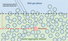 |
Fig. 1 Key model idea: a monomer of radius sm embedded at some monomer depth zm inside a home aggregate of effective radius sa. |
2.1 Background disk model
The processes which alter the ice mantle of the monomer all depend on the local disk environment as characterized by the spatial physical, thermal and chemical structure of the disk. For this purpose we utilize the thermochemical disk model ProDiMo (Woitke et al. 2009; Kamp et al. 2010; Thi et al. 2011, 2013). This code has been developed to calculate the local physical, thermal, and chemical structure in an azimuthally symmetric disk. We use ProDiMo to determine the local gas and dust density ρg, ρd, and temperature Tg, Td, respectively. Time-dependent chemistry in ProDiMo also allows us to infer the local molecule number densities nx of all species x. We here select molecular species based on their importance for the solid-phase CHNOS mass budgets. Therefore, we will restrict ourselves to volatile H2O, CO, CO2, CH4, NH3, and H2S throughout the rest of this work. Lastly, we use the local UV radiation field χRT, which is calculated from the 2D radiative transfer model.
The gas density structure of the disk is calculated from a parametrized column density structure (Woitke et al. 2009, 2016).
![Mathematical equation: ${{\rm{\Sigma }}_{\rm{g}}}\left( r \right) = {{\rm{\Sigma }}_0} \cdot \,{r^{ - }} \cdot \,\exp \,\left[ {{{\left( {{r \over {{r_{{\rm{taper}}}}}}} \right)}^{2 - \gamma }}} \right],$](/articles/aa/full_html/2023/06/aa45537-22/aa45537-22-eq1.png) (1)
(1)
where ϵ is the density profile power law index, and rtaper denotes the tapering radius beyond which an exponential cutoff occurs. Σ0 is derived from the normalization condition
 (2)
(2)
The vertical gas density structure is given by a Gaussian
 (3)
(3)
Here, Hg denotes the gas scale height, H0 the reference scale height at a reference distance r0, and β is the flaring exponent. The normalization ρ0 is determined via
 (4)
(4)
where zmax(r) = 0.5r is the maximum vertical height considered in the model (Woitke et al. 2009).
The initial dust density structure is treated in a similar fashion, where the total unsettled dust density  is related to the gas density as
  . Here, δ denotes the dust-to-gas mass ratio. However, we do account for the settling of the largest dust grains via the procedure outlined in Woitke et al. (2016). We assume that the initial unsettled dust size distribution follows the same power law everywhere in the disk:
![Mathematical equation: $f\left( a \right)\,\,\,\left\{ {\matrix{ { \propto {a^{ - {a_{{\rm{pow}}}}}}} \hfill & {{\rm{if}}\,a\, \in \,\left[ {{a_{\min }},{a_{\max }}} \right]} \hfill \cr { = 0} \hfill & {{\rm{elsewhere}}{\rm{.}}} \hfill \cr } } \right. $](/articles/aa/full_html/2023/06/aa45537-22/aa45537-22-eq7.png) (5)
(5)
Here, amin = 5 × 10⁻⁸ m denotes the minimum grain size. Similarly, amax denotes the maximum grain size, which is usually determined by the behaviour of local collisional growth processes. However, we note that grain growth in the outer regions of older disks may become drift-limited instead (Birnstiel et al. 2012). Assuming dust fragmentation by turbulence-driven relative motion, Birnstiel et al. (2012) expressed the maximum grain size as
 (6)
(6)
Here, ƒf denotes an offset parameter of order unity, which is assumed  throughout this work. ρa denotes the density of dust aggregates, and is assumed equal to the home aggregate density. α represents the turbulence strength (Shakura & Sunyaev 1973). υfrag denotes the relative velocity above which aggregates undergo fragmentation, while cs denotes the local isothermal soundspeed.
The proportionality constant in Eq. (5) is determined by requiring the total mass density resulting from integrating over all grain sizes a to be equal to the total unsettled dust mass density  (Woitke et al. 2016)
 (7)
(7)
Here, ρm = 2094 kg m−3 denotes the dust grain material density, which is assumed equal to the monomer density. The monomer and dust aggregate density ρa are related as ρa = ϕρm, where ϕ denotes the dust aggregate mass filling factor.
The grain sizes are sampled log-uniformly over Nbins = 100 size bins i between amin and amax,D. Here amax,D denotes the largest value for amax encountered anywhere throughout the disk, as calculated via Eq. (6). Subsequently, the dust scale height for each size bin is calculated via (Dubrulle et al. 1995)
 (8)
(8)
Here, St denotes the Stokes number, which is a function of grain size, soundspeed and the gas density in the disk midplane (see also Sect. 2.2). We note that Eq. (8) is similar to the relation between Hd and Hg derived by Youdin & Lithwick (2007). Dust only redistributes vertically, such that the surface density associated with a grain of size a at given radial distance r
 (9)
(9)
remains constant before and after settling.
The thermal structure of the gas and dust, and the local UV radiation field χRT are derived from the local 2D radiation field Jν, which is calculated with ProDiMo’s radiative transfer module. The gas temperature Tg and dust temperature Td are treated separately. The dust temperature is found by assuming radiative equilibrium for the dust, while the gas temperature is derived from a detailed heating/cooling balance. For a full description of the radiative transfer and heating and cooling model we refer the reader to Woitke et al. (2009, 2016); Thi et al. (2011); Aresu et al. (2011) and Oberg et al. (2022).
We use the time-dependent chemistry in ProDiMo to calculate the local gas phase molecule number densities nx of molecular species x. In the models used in this work, we considered the large DIANA chemical network containing 13 elements and 235 species. Within this chemical network, ions and ices of a particular molecular species are treated as different chemical species. Furthermore, we use the adsorption energies listed in the 2012 edition of the UMIST database (McElroy et al. 2013). However, we note that it is not possible to define a single set of adsorption energies which is consistent throughout the entire disk due to the different binding energies associated with different grain surface compositions (Kamp et al. 2017). For a more elaborate discussion of this specific chemical network, we refer the reader to Kamp et al. (2017), whereas the treatment of chemistry in ProDiMo has been discussed in Woitke et al. (2009); Aresu et al. (2011).
We use a two-step approach for the chemistry. The first step involves solving the time-dependent chemistry from initially atomic chemical abundances under molecular cloud conditions. We here choose an integration time of 1.7 × 10⁵ yr, where we follow Helling et al. (2014). This value has previously been derived as the best-fit lifetime for the Taurus Molecular Cloud 1 (McElroy et al. 2013). During the second step, we use the resulting abundances from this first step as initial chemical abundances for our disk model, and subsequently evolve this for another 2 × 10⁵ yr under the local disk conditions to yield representative chemical abundances at the onset of planetesimal formation. Although time-dependent chemistry is used to inform the chemical structure of the background disk models during the simulations, the local chemical abundances in the background models are kept fixed during SHAMPOO simulations.
Throughout this work, we consider four different background disk models, distinguished by the radial behaviour of amax outlined in Fig. 2. For three of these models, the radial behaviour of amax is given by Eq. (6) for a fragmentation velocity υfrag = 1, 5, 10 m s−1. We will refer to these models as vFrag1, vFrag5, and vFrag10. Furthermore, we also consider a background model const where the maximum grain size is fixed as a function of r to amax = 3 × 10⁻³ m. For all other disk model parameters, we consider the values listed in Table 1 for all four background models. These parameters are primarily setto values of the typical T Tauri model of the DIANA project (Woitke et al. 2016, 2019; Kamp et al. 2017; Dionatos et al. 2019). We also used this DIANA T Tauri model to inform our value for amax = 3 × 10⁻³ m for the const-model. However, it is thought that the onset of the formation of the first generation of planetesimals starts in the class I disk stage (e.g. Nixon et al. 2018). Therefore, we consider a more massive disk around a younger, more luminous pre-main sequence (PMS) star with respect to the standard T Tauri model parameters (Mdisk = 0.1 M⊙, L⋆ = 6 L⊙). This luminosity is consistent with a 0.7 M⊙ PMS star of 2 × 10⁵ yr and solar metallicity Z⊕ ≈ 0.02 (Siess et al. 2000).
The above approach gives rise to the disk structures depicted in Figs. A.1–A.4, which show the density (ρg, ρd) and thermal (Tg, Td) structures besides the UV radiation field;χRT for the four different background models. Furthermore, Figs. A.5–A.8 show nx as a function of position in the disk for H2O, CO, CO2, CH4, NH3, and H2S for the different background disk models, both in the gas and solid phase at the end of the evaluation of the time-dependent chemistry in ProDiMo. Qualitatively, the main differences between the background models are caused by the degree of settling, with background models with larger dust grains (vFrag5 and vFrag10) having their dust settled in a thinner disk compared to the gas density structure, which is identical for all four background disk models. In particular for the vFrag10-model, Fig. A.4 shows that ρd is significantly higher in the disk midplane due to settling, at the cost of lower values at higher z/r. As a consequence of dust settling, the midplane region which is shielded from UV radiation is thinner in disk models where amax is larger. This results in higher temperatures Tg, Td down to lower z/r, which also limits the ice-forming region towards lower z/r.
Input parameters used in the background disk model.
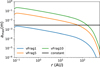 |
Fig. 2 Radial behaviour of amax for the four different background models considered throughout this work. |
2.2 Dust dynamics
The key purpose of the dynamical model is to describe the evolution of the radial (r) and vertical (z) position of the monomer during every time step ∆t. Key processes which can displace the monomer and its home aggregate are aerodynamic drag and turbulent diffusion. Our model is based on the work of Ciesla (2010, Ciesla 2011). The dynamical behaviour of the monomer is fully determined by the properties of its home aggregate, and by how well the home aggregate is coupled to the gas. An important measure which characterizes the nature of how the home aggregate interacts with the surrounding gas is the Stokes number (e.g. Armitage 2010; Krijt et al. 2018; Visser et al. 2021):
 (10, 11)
Here, ρa and sa denote the material density and size of the home aggregate. In addition, ρg and cs denote the local gas density and isothermal soundspeed. Ω denotes the Keplerian orbital frequency
 (12)
(12)
where G is the gravitational constant and M⋆ the mass of the host star. In addition, λmfp denotes the mean free path and is calculated as
 (13)
(13)
where µ = 2.3 denotes the mean molecular weight in atomic mass units, mp the proton mass, and σmol = 2 × 10⁻¹⁹ m2 the mean molecular cross section (see e.g. Okuzumi et al. 2012; Krijt et al. 2018).
As the Stokes number is a measure of how decoupled the motion of the home aggregate is from the gas, it can be used to characterize the dynamical behaviour of the home aggregate due to aerodynamic drag. The radial and vertical velocities due to aerodynamic drag υr and υz are given by (e.g. Armitage 2010)
 (14)
(14)
 (15)
(15)
η here denotes the dimensionless gas pressure gradient, given by
 (16)
(16)
Altogether, if a monomer is embedded in a home aggregate with significant Stokes number (St ≳ α), the monomer will move towards the disk midplane and radially inward as a consequence of the vertical settling and radial drift of the home aggregate.
In turbulent disks, aerodynamic drift can be countered by turbulent diffusion. Using the single-particle random walk formalism from Ciesla (2010, 2011), we calculate the new radial and vertical positions of the home aggregate and monomer after timestep ∆t as:
 (17)
(17)
 (18)
(18)
Here, R1 and R2 are uniformly drawn random numbers R1, R2 ∊ [−1, 1]. ξ denotes the variance of the distribution from which R1 and R2 are drawn, which means in our case that ξ = 1/3 (Visser 1997; Ciesla 2010). υr,eff and υz,eff denote the effective radial and vertical velocities, respectively, and are given by
 (19)
(19)
 (20)
(20)
Dd denotes the dust diffusivity and is calculated from the gas diffusivity Dg (Youdin & Lithwick 2007)
 (21)
(21)
We here estimate the gas diffusivity Dg with the turbulent viscosity, Dg = νturb = αcsHg (Shakura & Sunyaev 1973).
As a test for our dynamical model, we consider the vertical motion of 103 monomers at fixed radius r = 10 AU in Fig. 3. Our testing approach is similar to Ciesla (2010) and Krijt & Ciesla (2016). We perform this test for monomers of three different sizes moving in the const-background disk model: A monomer of radius sm = 5 × 10⁻⁸ m, sm = 3 × 10⁻⁴ m, and 3 × 10⁻³ m. At r = 10 AU and z/r = 0, the midplane Stokes numbers associated with these monomer sizes are St ≈ 1.9 × 10⁻⁷, 1.2 × 10⁻³, and 1.2 × 10⁻², respectively. These three monomers correspond to a fully coupled case (St ≪ α), a partially coupled case (St ~ α), and a more decoupled case (St > α). The integration time for each monomer was chosen to be 1.1 × 10⁵ yr, with a constant timestep of 1 yr. This timestep is at least a factor 100 shorter than the turbulent stirring timescale and the settling timescale associated with the largest particles. Since the turbulent mixing timescale at r =10 AU is roughly 104 yr, we omitted the first 104 yr of each monomer trajectory from Fig. 3 (see Sects. 2.5 and 3.1).
The total time that these monomers spend at each height z/r should be proportional to the background density profile of dust particles with the same Stokes number, which is a Gaussian profile with its standard deviation given by the dust scale height (Eq. (8)). Figure 3 shows that this holds for the smallest monomers (5 × 10⁻⁸ m) and largest monomers (3 × 10⁻³ m), whereas Eq. (8) appears to overestimate the width of the density profile of intermediate-sized monomers (3 × 10⁻⁴ m). This deviation was also found by Krijt & Ciesla (2016), and is a consequence of Eq. (8) not taking into account variations in the Stokes number as a function of height z/r (Ciesla 2010), whereas it is in our model.
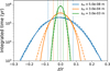 |
Fig. 3 Integrated residence time for monomers of sm = 5 × 10⁻⁸ m (blue), 3 × 10⁻⁴ m (orange), and 3 × 10⁻³ m (green) as a function of height z at r = 10 AU. The solid lines denote the histogram obtained from the trajectories of 103 monomers combined, whereas the dashed lines are the theoretical vertical density profiles expected from Eq. (8). The vertical dashed lines depict the locations where z = Hd for each monomer size. |
2.3 Collisions
With the collision model, we aim to track the evolution of the home aggregate size sm and monomer depth zm as the home aggregate is altered by coagulation, fragmentation, and erosion. We here treat collisions in a similar fashion as Krijt & Ciesla (2016), i.e. collisions are allowed to occur randomly, while we track the effect of each collisional interaction on the home aggregate size sm. In addition, we use a simple probabilistic model to determine the new monomer depth zm after a collision has occurred. Thus, during every global time step ∆t, we first determine probabilistically whether a collision has occurred, and if so, what the effects are on the size of the home aggregate sa and on the depth at which the monomer is located zm.
In order to determine the probability of a collision occurring during time step ∆t, we are required to evaluate the collision rates for a given home aggregate of size sa with any other particle size bin present in our background dust size distribution. The collision rate for the home aggregate with a particle of size bin i is
 (22)
(22)
Here, ni denotes the local number density of particles of size bin i, σcol = π(sa + si)2 and υrel, the relative velocity between the home aggregate and the collision partner. We relate ni to the partial disk surface density associated with particles from size bin i, Σd,i
 (23)
(23)
Here, Hd,i denotes the dust scale height associated with dust particles from size bin i. We can obtain the total dust surface density Σ from Σd,i via
 (24)
(24)
The total relative velocity υrel associated with a collision between the home aggregate and a given collision partner constitutes contributions from Brownian motion (υBM), differential aerodynamic drag consisting of radial drift (υr), vertical settling (υz), azimuthal drift (υϕ), and turbulent motion (υturb) (Birnstiel et al. 2010; Krijt et al. 2016b).
 (25)
(25)
Following the approach of Krijt et al. (2016b), we calculate the relative velocity due to Brownian motion as
 (26)
(26)
Here  denotes the mass of the home aggregate (with ρa denoting the mass density of the home aggregate), and mi denotes the mass of a collision partner from size bin i. All dust grains, whether part of a size bin or a monomer have equal material density.
Differential aeorodynamic drag constitutes a radial (υr), vertical (υz), and azimuthal (υϕ) component, given by:
 (27)
(27)
 (28)
(28)
 (29)
(29)
Here, υr,n and υz,n (n ∊ (a, i)) are calculated from Eqs. (14) and (15), respectively. Sta denotes the Stokes number associated with the home aggregate, while Sti denotes the Stokes number of the collision partner.
For the contribution of turbulence to the total relative velocity, we use the approach derived by Ormel & Cuzzi (2007):
 (30)
(30)
Here,  denotes the mean random velocity of the largest turbulent eddies (Krijt et al. 2016b). The value of Q depends on how the stopping time ts = St/Ω compares to the orbital period 1/Ω and the turnover timescale of the smallest scale eddies,
  :
:
 (31)
(31)
Here, we associate the Stokes number St1 with the largest particle, either being the home aggregate or the collision partner, and St2 with the smallest of the two. Re denotes the turbulent Reynolds number, which we calculate as the ratio between the turbulent viscosity νturb and molecular viscosity νmol:
 (32)
(32)
The above calculations are performed for every size bin i, to find the associated Ci via Eq. (22). Subsequently, the total collision rate Ctot can be obtained via
 (33)
(33)
such that the probability of a single collision event happening during timestep ∆t is
 (34)
(34)
Because this expression does not incorporate the possibility of multiple collisions, we are required to set ∆t shorter than the timescale for a single collision, ∆t ≲ 1/Ctot. This can become a problem if our home aggregate is large and located near the midplane. In this situation, the home aggregate will collide frequently with (sub)miron-sized grains, resulting in Ctot becoming very large (Krijt & Ciesla 2016).
To prevent the usage of prohibitively small values of ∆t, we group collisions with collision partners which have a mass mi which is smaller than a fraction ƒc = 10−1 of the home aggregate mass ma (Ormel & Spaans 2008; Krijt et al. 2015; Krijt & Ciesla 2016). Instead of treating each collision between the home aggregate and small collision partners separately, we only allow the home aggregate to collide with a group of small collision partners at once. The effective collision rate for such a group collision will be (much) smaller than the collision rate between the home aggregate and the individual collision partners which constitute the group. We express the number of particles per group Ncol as
 (35)
(35)
such that the modified collision rates become
 (36)
(36)
We then calculate the modified total collision rate as
 (37)
(37)
such that the probability of a collision occurring during a timestep ∆t is
 (38)
(38)
To determine whether a collision event occurs during a timestep, we generate a random number R3 ∊ [0, 1], such that if R3 ≤  , the monomer has undergone a collision event.
In order to determine the effect of a collision on the monomer and home aggregate, we first need to determine the mass of the collision partner, which we determine by generating another random number R4 ∊ [0,  ], and sum over the various collision size bins up to bin n, which is the first bin which satisfies
 (39)
(39)
We then select a particle from size bin n as the collision partner. Note that this automatically means that size bins which have a higher associated collision rate are more likely to be selected.
The outcome of a collision is fully determined by the mass ratio of the collision partner and the home aggregate, and their sizes. The first step of determining the collision outcome is whether the collision is constructive (net dust growth) or destructive (net dust fragmentation). We assume that the probability of a collision event resulting in fragmentation Pfrag can be fully expressed in terms of the relative velocity υrel (Birnstiel et al. 2011):
 (40)
(40)
We here defined δυfrag = υfrag/5, where we follow Birnstiel et al. (2011). After the collision partner and Pfrag have been determined, we generate a random number R5 ∊ [0, 1]. A destructive collision will occur if R5 ≤ Pfrag.
Regardless of collision outcome, we need to re-calculate the home aggregate mass and size, ma and sa, after each collision event. In addition, different collision events have an effect on the depth at which our monomer is embedded, zm. We distinguish between the following collision outcomes:
1. Coagulation. In this case, R5 > Pfrag and the collision event results in the coagulation of the home aggregate and the collision partner(s) of mass mc. The new home aggregate mass ma,new then follows from
 (41)
(41)
Note that if mc/ma,old > ƒc, the group size is Ncol = 1 (Eq. (37)). The new monomer depth zm,new is calculated as
 (42)
(42)
where sa,old and sa,new denote the old and new home aggregate size, respectively. Effectively we thus assume that the mass of the collision partner(s) is added to the old home aggregate as a homogeneous surface layer, such that the monomer is buried deeper inside the new home aggregate.
2. Fragmentation. In this case, the home aggregate is catas-trophically disrupted by the collision partner, which must be similar to the home aggregate in terms of mass:
 (43)
(43)
The new home aggregate of the monomer becomes one of the fragments produced during the collision. We assume these fragments follow the distribution (Birnstiel et al. 2010)
 (44)
(44)
where ξfrag = 1.83 (Brauer et al. 2008). In addition, mmax denotes the maximum possible fragment mass. In the case of fragmentation, we set mmax = max(ma, mc). We draw the new monomer depth zm,new from a spherically uniform distribution, such that the probability P(zm,ew) of the monomer being located at a certain depth after a destructive collision is proportional to the home aggregate mass density ρa. This means that the monomer is more likely to be located close to the surface after a fragmentation event since P(zm) ∝ (sa − zm)2. In reality, the functional form P(zm,new) is likely set by the size of the original home aggregate sa,old size of the collision partner sc and their relative velocity υrel (Dominik & Tielens 1997).
3. Erosion. Erosion occurs when mc/ma,old ≤ ƒc, as the collision partner is too small to result in full fragmentation of the home aggregate. Instead, the collision partner exhumes and ejects mass of the home aggregate. We here follow Krijt & Ciesla (2016) and assume that the mass ejected is mej = 2mc. In order to determine whether the monomer is ejected, we define the ejection probability Pej
 (45)
(45)
and generate another random number R6 ∊ [0, 1], such that the monomer is ejected if R6 ≤ Pej.
Ejection. In this case the new home aggregate is one of the fragments ejected, whose mass is selected according to Eq. (44). In this case, we set mmax = mc, and also draw the new monomer depth zm from a spherically uniform distribution.
-
No ejection. If the monomer remains in its old home aggregate, the new lower home aggregate mass ma,new and smaller monomer depth zm,new are calculated via
 (46)
(46)
 (47)
(47)This means that the monomer depth decreases as mass is removed isotropically from the surface.
4. Impact. In this case mc/ma,old ≥ ƒc, which means that the home aggregate is impacting and eroding the considerably larger collision partner. We here assume that the ejected material only originates from the collision partner, such that the new home aggregate becomes the collision partner, whose mass is
 (48)
(48)
Again, we assume that the collision results in major restructuring of the new home aggregate, which is why we again use a spherically uniform distribution to determine a new value for the monomer depth zm.
We consider a test similar to the one performed by Krijt & Ciesla (2016). Since tracking a monomer effectively entails tracking a unit of mass, the fraction of time which monomers spend inside aggregates of a given size sa, when summed over many individual monomer histories, must be proportional to the background local dust mass density as a function of grain3 size a = sa, ρd(a, r, z). We compare the total integrated monomer residence time of 6000 monomers to the vFrag5 background model grain size distribution ρd(a, r, z) for monomers in aggregates with fragmentation velocities of υfrag = 1, 5, 10m s−1. All monomer positions are kept fixed at r = 10 AU and z/r = 0, and initially assumed to be bare, such that the initial home aggregate size is always sa = sm = 5 × 10⁻⁸ m. Furthermore, the aggregate density is assumed equal to the monomer density (i.e. ρa = ρm, corresponding to a filling factor ϕ = 1). Each simulation is run for 110 kyr, where we exclude the first 10 kyr of each simulation from the analysis such that we can neglect effects of our initial choice of home aggregate size. The timestep is set to ∆t = 10 yr, which is several orders of magnitude below the total group collision rate  at 10 AU (see Sects. 2.5 and 3.1).
The integrated monomer residence times shown in Fig. 4 follow the background density distribution for all three fragmentation velocities υfrag quite well for small aggregates up to ~3 × 10⁻⁴ m. In addition to the integrated monomer time in Fig. 4, we also report the total number of occurrences of the different collision outcomes for all 6000 monomers in Table 2.
For all three fragmentation velocities, the residence time shows a small dip at ~3 × 10⁻⁵ m. This results from the stopping time associated with this aggregate size becoming larger than the turnover timescale of the smallest scale eddies tη (Eq. (31)), resulting in a sudden increase in the relative velocity due to turbulence (Ormel & Cuzzi 2007), which increases the collision rates associated with aggregates of sa ~ 3 × 10⁻⁵ m. Therefore, these aggregates are depleted in a similar fashion as the smallest aggregates. We note that both the stopping time and tη depend on the local disk gas density ρg and soundspeed cs. This means that the location of this dip depends on position in the disk.
Above sa ~ 3 × 10⁻⁴ m, the integrated residence time starts to deviate significantly from the background grain size distribution for all three values of υfrag. This is primarily due the fact that although our background grain size distribution incorporates settling, it does not directly account for the effects of collisions. For υfrag = 1 m s−1 and υfrag = 10 m s−1, the peak in the residence time occurs respectively for aggregate sizes smaller or larger than the maximum grain size of the background grain distribution. This is expected since the maximum grain size in the background model is calculated for υfrag = 5 m s−1. For υfrag = 1 m s−1, aggregates larger than ~3 × 10⁻⁴ m should not be able to form (Fig. 2). This size limit is indeed the location of the peak in monomer residence time in Fig. 4. However, the maximum grain size at 10 AU in the vFгag5-model is amax ≈ 1 × 10⁻² m, which means that aggregates are still colliding with grains above the maximum aggregate size allowed by the collision model. Such a collision would occur at a relative velocity higher than υfrag = 1 m s−1, although it is still possible for the monomer to end up in the larger collision partner via an impact event. Table 2 shows that for the monomers in aggregates with υfrag = 1 m s−1, impact events occur frequently. This can explain why such monomers still spend a considerable amount of time in aggregates with sa ≳ 3 × 10⁻⁴ m. Such aggregates would have a short lifetime, as in this size regime only destructive collisions are possible. This also explains why the monomers in aggregates with υfrag = 1 m s−1 undergo significantly more fragmentation, erosion, and ejection events than monomers in aggregates with υfrag = 5, 10 m s−1 (Table 2).
For monomers in aggregates with υfrag = 10 m s−1, the aggregate is allowed to grow to sizes beyond the local value of amax ≈ 1 × 10⁻² m in the background model. In this case, there are no grains of similar size present in the background model at r = 10 AU and z = 0, which means that the aggregate can continue to grow, primarily through the sweep-up of many groups of smaller grains. Similarly, when relative velocities start to exceed υfrag = 10 m s−1, aggregates have grown to such an extent (up to sa ~ 4 cm) that collisions with similarly-sized grains almost never occur. Table 2 indeed shows no fragmentation events for monomers in aggregates with υfrag = 10 m s−1, indicating that only erosion by many groups of small grains is a viable mechanism to limit further growth of the aggregate. However, Fig. 4 shows that this does not prevent monomers from spending a significant amount of time in aggregates larger than amax.
For the case υfrag = 5 m s−1, which is consistent with the value for amax calculated in the background model, the integrated residence time and ρd are in good agreement for almost all grain sizes. However, some differences between the integrated monomer residence time and ρd(α) still remain. The former shows a deficit with respect to ρd(α) in the size regime below amax = 1 × 10⁻² m, and also shows a small excess of time where monomers reside in aggregates larger than the maximum grain size in the background model amax. In the collision model, the aggregate size is allowed to peak at sizes for which υrel > υfrag. However, these aggregates are very short-lived, as collisions tend to result in fragmentation or erosion of such a large aggregate. This may also explain the significant number of fragmentation, ejection, and erosion events in Table 2 for υfrag = 5 m s−1. The formation of aggregates larger than amax may come at the cost of the number of aggregates between sa ~ 3 × 10⁻⁴ m and amax, as these are preferentially growing to aggregates slightly above amax with respect to the background model. Altogether these discrepancies appear to result from the fact that the grain size distribution in the background model is approximated with a power law distribution (Eq. (5)), modified by the effects of settling. Furthermore, the grain density drops to zero in the first size bin above amax(r). However, this may be incorrect near the peak of the grain size distribution, where a dust size distribution limited by turbulence-driven fragmentation generally departs from a power law such as the one assumed in the background model (Birnstiel et al. 2011; Krijt & Ciesla 2016).
Altogether our collisional model is able to reproduce the background dust size distribution which is most consistent with the fragmentation velocity used in our model. As illustrated above, the usage of a background dust size distribution which is not automatically consistent with the collision model can induce errors in the collisional histories of individual monomers. This occurs when there is a difference between the fragmentation velocity in the collision model and the fragmentation velocity which determines the maximum grain size amax at a given position in the background model (Eq. (6)). The key variable affected is the home aggregate size sa, specifically the average time a monomer spends in home aggregates of a given size. Furthermore, discrepancies between the value for υfrag used in the collision model and the value used to calculate amax in the background model also affect the frequencies of different collision outcomes. Both of these errors propagate into the monomer depth zm, which in turn can affect the ice evolution of the monomer (see also Sect. 4.2). Therefore, it is key to ensure that the background model dust size distribution ρd(a, r, z) is as consistent as possible with the assumptions in the collision model, such as the fragmentation velocity υfrag.
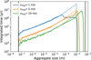 |
Fig. 4 Integrated monomer residence time as a function of home aggregate size for different fragmentation velocities (solid coloured lines). The solid black lines on the left and right represent the minimum and maximum grain size occurring throughout the entire vFrag5 background disk model. The dashed lines all denote the same background dust mass distribution as a function of size, ρd(a) at r = 10 AU and z = 0, shifted vertically for comparison with the integrated monomer residence time. |
2.4 Ice evolution
The ice evolution model tracks the amount of ices of different species present in the ice mantle around the monomer. We here only track the ice composition of the monomer as it travels through the disk and is constantly changing home aggregate. Therefore, we aim to develop a stochastic approach for how the fluxes of volatile molecules and photons impinging onto the home aggregate affect the ices associated with the monomer. A crucial parameter in regards to both is how deep the monomer is embedded inside the home aggregate, zm (see Fig. 1). A monomer close to the surface (zm ~ sm) can more easily acquire an ice mantle from impinging molecules than a monomer buried beneath many layers of other monomers (zm ~ sa ≫ sm). However, such a buried monomer would also be more protected from photodesorption by the overlying monomers, which would absorb any incident UV radiation. If we assume that the local disk environment allows molecules to approach the home aggregate in straight lines (i.e. if the aggregate is in the Epstein regime), the monomers at z < zm can be treated as a slab of particles each of size sm, absorbing individual impinging molecules and photons. From a radiative transfer viewpoint, each geometrical monomer depth zm can be associated with an optical depth τ defined as
 (49)
(49)
Here, σ denotes the collision cross section, and nm the monomer number density. We approximate the collision cross section with the monomer cross section  , where we neglect the molecular cross section in case of impinging molecules. However, we note that this may be inappropriate for large molecular complexes which are similar in size to the monomer. Assuming constant monomer density throughout the home aggregate, we can estimate nm as
 (50)
(50)
where ϕ denotes the home aggregate mass filling factor and  denotes the monomer mass, such that Eq. (49) becomes
 (51)
(51)
For an isotropic radiation field, the fraction of radiation which can reach down in the slab to an optical depth τ can be written as (e.g. Whitworth 1975)
 (52)
(52)
Here, E2 denotes the exponential integral, and represents the spatially averaged fraction of all impinging molecules and photons which can reach down to depth zm in the home aggregate. Note that the above equations strictly apply when sa ≫ sm, and that the home aggregate has a fractal dimension Df = 3, such that  .
.
Although E2 represents the fraction of molecules and photons which can reach down to a given optical depth τ, the actual flux of molecules and photons received by an individual monomer does not have to scale with E2(τ). Monomers may be arranged in fractal and clustered configurations inside the home aggregate as a consequence of initial hit-and-stick growth followed by compaction (e.g. Dominik & Tielens 1997; Wurm & Blum 1998; Weidling et al. 2009). This means that some monomers at depth zm may lie completely in the shadow of other monomers, whereas other monomers at depth zm may be fully exposed as there are no other monomers blocking incoming molecules and photons that travel inside the home aggregate effective radius sm. Although full modeling of this spatial flux distribution is beyond the scope of this paper, we account for this behaviour by interpreting Eq. (52) as an exposure probability Pexp: the probability that a monomer, located at a depth zm, is exposed to the outside environment. Being exposed as a monomer here means that the monomer ice mantle is able to undergo adsorption or photodesorption. Altogether we define the exposure probability as
 (53)
(53)
We here define the critical monomer depth zcrit = 2sm = 10−7 m to ensure that monomers which are closer to the surface than the diameter of a single monomer are always exposed, regardless of filling factor ϕ. Fig. 5 shows the value of Pexp as a function of zm for different values of ϕ. The filling factor is here varied from ϕ = 1 to ϕ = 10−5. Such a low value for ϕ is thought to be possible for aggregates grown through efficient sticking and inefficient fragmentation, which results in very fluffy aggregates (Okuzumi et al. 2012; Kataoka et al. 2013). For a filling factor of 10−5, it appears that molecules and photons have a significant chance to reach monomers which are embedded in the center of even the largest aggregates, amounting to more than 30% for sa = 10−3 m. For larger filling factors, monomers in the center of large aggregates are mostly shielded from gas phase molecules and photons.
To model the evolution of the composition of the ice mantle of the tracked monomer we solve at each time step the following mass balance equation for each chemical species x to find the change in ice mass of that species Mx:
 (54)
(54)
Here, R7 ∊ [0, 1] denotes a random number from a uniform distribution we generate after each collision event to determine whether the monomer is exposed. Furthermore, ℛads,x denotes the specific adsorption rate (in kg m−2 s−1), ℛads,x the specific thermal desorption rate, and ℛpds,x the specific photodesorption rate associated with species x. The factors  in Eq. (54) associated with ℛads,x and ℛpds,x follow from the assumption that on average, impinging molecules are only effectively adsorbed on the monomer hemisphere aimed towards the aggregate surface, whereas the same applies for photodesorption by impinging UV photons. We treat the ice transport processes as follows:
-
Adsorption. Molecules in the gas phase can collide and stick to the monomer, such that the specific adsorption rate (in kg m−2 s−1) for species x is given by the product of the molecule collision rate and sticking probability:
 (55)
(55)Here, nx denotes the gas phase molecule number density (in m−3), mx the molecular mass of species x. υth,x denotes the mean thermal speed of species x and is calculated as (Woitke et al. 2009)
 (56)
(56)S denotes the sticking probability. We calculate S using the expression of He et al. (2016)
![Mathematical equation: $S = {\alpha _S}\left[ {1 - \tanh \left( {{\beta _S}\left[ {{T_{\rm{d}}} - {\gamma _S}{{{E_{{\rm{ads,}}x}}} \over {{k_{\rm{B}}}}}} \right]} \right)} \right].$](/articles/aa/full_html/2023/06/aa45537-22/aa45537-22-eq70.png) (57)
(57)Here, αS, βS, and γS are fitting parameters, which have been derived for experimental data on the sticking of H2, D2, N2, O2, CO, CH4, and CO2 on amorphous, nonporous water ice (He et al. 2016). We note that αS = 0.5 for all species to ensure 0 ≤ S ≤ 1, while the values of βS and γS depend on molecule species. However, experimental data on βS and γS for the sticking of different chemical species on different surfaces is limited. Therefore, we follow He et al. (2016) and use βS = 0.11 K−1 and γS = 0.042 for all species as an approximation.
-
Thermal desorption. We express the thermal desorption rate ktds,x for species x as
 (58)
(58)Here, νx denotes the ice lattice vibration frequency (Tielens & Allamandola 1987; Cuppen et al. 2017):
 (59)
(59)Nads = 1019 m−2 denotes the density of adsorption sites on the monomer surface. Furthermore, Eads,x denotes the adsorption energy associated with species x. The specific thermal desorption rate for an ice species x can be expressed as (Cuppen et al. 2017)
 (60)
(60)Here, Nact is the number of actively desorbing ice molecule monolayers. Typical values for Nact range from 2 to 4 (Cuppen et al. 2017), which motivated using a median value of 3 in this work. We express the ice fraction ƒx in terms of mass:
 (61)
(61)Here, Mx denotes the total mass of species x present in the monomer ice mantle.
-
Photodesorption. We treat photodesorption in a similar fashion as Woitke et al. (2009), and write the specific photodesorption rate as
 (62)
(62)Here Y = 1 × 10⁻³ denotes the UV photon yield, and χFDraine denotes the local UV radiation field strength in photons m−2 s−1.
In the above treatment, the escape of molecules from the home aggregate is not modelled. However, molecules liberated by thermal desorption from the ice mantles of monomers located at large τ collide with a significant number of other monomers before escaping back into the gas phase, which can result in re-adsorption if the sticking probability S > 0. We explore the timescale associated with molecule escape and the concept of re-adsorption in Appendix B. We find that re-adsorption may be important for particular molecular species in a comparatively small region immediately behind the iceline of the respective molecular species. Thus, our model could underestimate the amount of ice from individual species retained on monomers at large τ in these disk regions.
As a numerical test for our model, we compare the trajectories of pure H2O monomer particles predicted by our model to the model of Piso et al. (2015). In our comparison, we consider particles which are allowed to undergo radial drift and thermal desorption. We here use the background disk structure and model parameters used by Piso et al. (2015).
The disk gas surface density is calculated as
 (63)
(63)
such that the midplane gas density becomes, when assuming a Gaussian vertical density profile
 (64)
(64)
Hg in this context is calculated as the pressure scale height Hg = cs/Ω. The soundspeed is obtained from the temperature profile (Piso et al. 2015)
 (65)
(65)
Note that since collisions, adsorption and photodesorption are not considered by Piso et al. (2015), the evolution of the particle is fully determined by the local gas density and temperature. Since the gas and dust temperature Tg are coupled in the midplane, we assume Tg,P = Td for this test. For radial drift, the dimensionless pressure gradient η (Eq. (14)) is estimated as
 (66)
(66)
The sound speed cs is calculated via
 (67)
(67)
where the dimensionless mean molecular weight is set to µP = 2.35 (Piso et al. 2015).
We also set the value of the adsorption energy for H2O,  to 5800 K, the same value as used by Piso et al. (2015). As a default value, we use the UMIST RATE12 value of 4800 K (McElroy et al. 2013). Furthermore, the particles have a density ρa = 2000 kg m−3, and a filling factor ϕ = 1. We calculate the ice lattice vibration frequency as (Hollenbach et al. 2009; Piso et al. 2015)
 (68)
(68)
while we calculate the specific thermal desorption rate ℛtds using Eq. (60) with  .
.
Figure 6 depicts the evolution of the monomer size as a function of time and H2O ice mass as a function of radial distance r for pure H2O grains with sizes of 10−3 m up to 10 m. We here compare the evolutionary trajectories predicted by our model with the trajectories depicted in the center row of Fig. 4 of Piso et al. (2015), where the same particles are released in the disk midplane at 10 AU. Note that for this test, the effects of turbulent diffusion on radial migration is neglected, such that aerodynamic drag is the only process affecting the radial position of particles.
Both the model of this work and the model of Piso et al. (2015) predict that regardless of initial particle size, the sublimation is almost instantaneous once a particle crosses the snowline. However, there appears to be a small difference in the time at which sublimation happens. For example, the model of Piso et al. (2015) predicts sublimation of a particle of 10−3m after 3 × 10⁶ yr, whereas the sublimation time in our model is 4 × 10⁶ yr. However, a more detailed analysis revealed that the most likely cause of this deviation is inaccuracies in the digitation software used to extract the data points from Fig. 4 of Piso et al. (2015). This is further strengthened by the agreement of the trajectories for the ice masses as a function of radial distance shown in the right panel of Fig. 6. The authors also note the high sensitivity of the sublimation time to changes in model parameters.
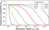 |
Fig. 5 Exposure probability as a function of monomer depth zm for different filling factors ϕ. |
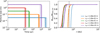 |
Fig. 6 Particle size as a function of time (left panel) and ice mass (scaled with the initial ice mass) as a function of radial distance (right panel) for pure H2O particles undergoing radial drift and thermal sublimation. Different colors denote different particles sizes. The trajectories predicted by the model of this work (solid lines) are compared with the trajectories calculated by Piso et al. (2015; dots). The vertical dashed line in the right panel denotes the position of the H2O iceline at 0.67 AU as calculated by Piso et al. (2015). |
2.5 Timescales
To enable us to spatially constrain the regions where disk processes are coupled, we will compare their associated timescales later in this work (Sect. 3.1). In this subsection we outline our approach to estimating these timescales.
For dynamical processes, we compare the radial drift, vertical settling, and turbulent mixing timescales, denoted by τrm, τzm, and τtm, respectively:
 (69)
(69)
Here, υr and υz denote the drift velocities due to aerodynamic drag, given by Eqs. (14) and (15), respectively, while νturb = αcsHg. We here choose the gas pressure scale height Hg as the length scale for the migration timescales (τrm, τzm) since Hg is the typical length scale associated with the turbulent mixing timescale τtm. For collision processes, the timescale over which a particle collides with a significant fraction of its own mass worth of collision partners can be estimated as
 (70)
(70)
Here the total group collision rate  is given by Eq. (37). We note that this definition differs from earlier work, where the timescale for collisional processing has been defined in terms of the time required for a particle to significantly change size as a function of the local dust-to-gas mass ratio (see e.g. Brauer et al. 2008; Birnstiel et al. 2012).
For ice formation, we consider the ice adsorption and desorption timescale for molecular species x as a function of position. We here estimate the average amount of ice present on a monomer from the solid phase number density predicted by the background model, nx,ice, as (Figs. A.5–A.8)
 (71)
(71)
The adsorption and desorption timescales, τads and τdes, respectively, are then given by
 (72)
(72)
 (73)
(73)
3 Results
As a first step, we use our model to constrain the disk regions where the dynamical, collisional and ice processes are highly coupled (Sect. 3.1). Subsequently, we demonstrate how the coupled behaviour of these processes affects the ice mantle composition of individual monomers (Sect. 3.2). For all monomer models, the parameter values denoted in Table 3 are used, unless noted otherwise.
3.1 Coupling analysis
As a starting point, we investigate the relative importance of the various grain transport processes. We explore the relative importance of turbulent stirring with respect to aerodynamic drift processes as a function of grain size in Fig. 7. Throughout this section, we consider the const-model as the background disk model for our analysis, which means that the maximum grain size amax = 3 × 10⁻³ m remains constant as a function of r. Furthermore, we always assume a filling factor ϕ = 1, such that the material density is always equal to the monomer density, ρa = ρm = 2094 kg m−3. Figure 7 highlights the physical grain size associated with St = 10−3 for the const background disk model discussed in Sect. 2.1. We here inverted Eqs. (10) and (11) to give the grain size as a function of Stokes number. Grains with St = 10−3 would undergo significant settling (Eq. (8)) for the turbulence strength parameter value used, α = 10−3. It becomes clear that the physical grain size associated with a fixed Stokes number varies greatly throughout the disk, ranging from ~10−2 m at the transition from the Epstein to the Stokes regime to ≲10−6 m in the outer disk and above z/r ~ 0.25. This is primarily a consequence of the background model gas density, which varies many orders of magnitude throughout the disk (Fig. A.1). A lower gas density decreases the coupling of dust grains to the gas, and hence increases the Stokes number of a dust grain of given size (Eqs. (10) and (11)). We note that the grain size associated with St = 10−3 can also vary as a function of gas temperature due to the dependence of the Stokes number on the soundspeed. However, this effect is much less pronounced in Fig. 7 due to two effects. The dependence of the Stokes number on the gas temperature is weaker than its dependence on the gas density ( compared to St ∝ 1/ρg). Furthermore, the variation in the gas temperature is small compared to the variation in the gas density, both radially and vertically (Fig. A.1). Despite the limited influence of the gas temperature, the dynamical behaviour of a dust grain of given size and its associated timescales can be expected to vary significantly as a function of position in the disk.
As a next step, we investigate the coupling behaviour of the timescales introduced in Sect. 2.5. As an example, we consider the radial behaviour of the timescales for radial drift, vertical settling, turbulent stirring, collisional growth, ice adsorption, and ice desorption in Fig. 8. The timescales are associated with a dust grain of 10−5 m with an H2O ice mantle. The vertical height is kept fixed at z/r = 0.05.
We find that in the inner disk (r ≲ 1 AU), the collisional growth timescale τcol becomes shorter than any dynamical timescale by at least an order magnitude, and drops even below ~10−1 yr at r = 0.1 AU. The shorter collision timescale for decreasing r is a result of the increasing dust density closer to the star, which in turn increases collision rates (Eq. (22)).
The turbulent stirring timescale τtm, although 1–3 orders of magnitude longer than τcol, is still far shorter than the aerodynamic drag timescales, τrm and τzm, which are between ~104 and ~106 yr for r ≲ 1 AU. This is a consequence of the rather small particle size in combination with a high gas density in the inner disk, which together result in a small Stokes number (≪10−3 Fig. 7), and hence low drift velocities.
For r ≳ 1 AU, almost all timescales initially increase as a function of r. In case of the dynamical timescales, the increase results from the increase of gas scale height Hg (Eq. (3)). However, beyond 10 AU, the lower gas density results in an increasing Stokes number, and therefore increasing drift velocities result in τrm and τzm gradually decreasing around r ≳ 100 AU, overtaking turbulent stirring as the fastest dynamical processes around r ~ 150 AU.
For r ≳ 1 AU, the ice formation timescales, τads and τdes both increase as a function of r. We define the H2O iceline as the position where τads = τdes. Although Fig. 8 indicates that τads and τdes are very similar for r ≲ 4 AU, this condition puts the H2O iceline at r ≈ 1.7 AU for z/r = 0.05. We note that both beyond the inner and outer boundary of the ice-forming region, τdes decreases. Interior to the iceline this is due to increased thermal desorption, while in the outermost disk regions this is a consequence of higher photodesorption rates. The radial behaviour of τads is primarily shaped by the local H2O gas abundance, which explains its rapid decrease interior to the iceline: as H2O ice sublimates interior to the iceline, the gas phase H2O abundance increases significantly in the background model (Appendix A.2). The rapid increase of τads for r < 1 AU is a consequence of the decrease in the sticking probability S.
In terms of coupling behaviour, it becomes clear that in the inner disk, the various disk processes are largely decoupled since τads,τads ≪ τcol ≪ τtm ≪ τrm, τzm, whereas dust dynamics, collisions, and ice processing become more coupled for increasing r up to r ≈ 20 AU. Beyond this distance, both τads and τdes become much larger than the other timescales, indicating that ice processing is very slow compared to collisional and dynamical processing in the outer disk regions.
It should be emphasized that this result only applies to a dust grain of size sm = 10−5 m with a pure H2O mantle. Since the collisional growth timescale is much smaller than the disk lifetime throughout most of the disk, it is expected that these dust grains will likely be incorporated rapidly into larger dust aggregates. Therefore, it is necessary to explore the coupling and decoupling of the various processes as a function of grain size, ice species, and also for the full extent of height z/r above the disk midplane.
Figure 9 explores the coupling of the various timescales as a function of both r and z/r in case of a dust grain of sm = 10−7 m (left panel) and sm = 10−3 m (center panel). For sm = 10−7 m, we also explore a case where we only allow a pure CO ice mantle to form instead of a pure H2O ice mantle (right panel). We highlight the disk regions where the various timescales obey various decoupling conditions. We here categorized the timescales in a dynamical (τrm,τzm and τtm), collisional (τcol), and ice processing τads,τdes group. The process with associated timescales τi then decouples from the other processes with associated timescales
 (74)
(74)
or
 (75)
(75)
Here we set fdec = 103 to encapsulate that we require a particular process to act much faster (Eq. (74)) or much slower (Eq. (75)) than the other disk processes. For ice processing, we only consider τads interior to the iceline, and τdes exterior to the iceline in this calculation.
In all three cases, ice desorption decouples from the other processes in any disk region radially interior to the ice forming region. This decoupling originates from the short desorption timescale, since thermal desorption and photodesorption are very efficient outside the ice forming region. We also find in the cases of H2O, ice formation can decouple from the other disk processes due to the low adsorption rate in the ice forming region (most clearly visible in the center panel of Fig. 9). This is primarily a result of the low gas phase abundance of H2O inside the ice forming region (Appendix A.2). The center panel of Fig. 9 shows that this effect is more pronounced for a large dust grain since more ice mass must be accumulated onto the grain surface to double the initial ice mantle mass (Eq. (72)).
In all three panels of Fig. 9 we discern a region towards the innermost disk midplane where the three groups of processes fully decouple. In this region, dynamical processes become much slower than collisional growth, which is due to the high collision rates in the inner disk (Fig. 8). The center panel of Fig. 9 also demonstrates that this region of full decoupling in the inner disk is smaller for larger dust grains. The shrinking of this region can be attributed to the fact that more collisions are required to result in a significant change in mass for a massive dust grain. Therefore, the effective collision rates become smaller, and hence τcol increases.
The most important features of Fig. 9 are the white regions in all three panels around the ice forming regions. For various species, all the three process categories couple to one another. However, the location of this fully coupled region is dependent on the grain size and position of the iceline. Since different grain sizes are connected via coagulation and fragmentation, and the position of the iceline depends on molecular species, there is no ubiquitously decoupled regime in the planet-forming region. In order to understand the ice composition of planetesimals, we thus require a modeling approach such as SHAMPOO which treats dynamical, collisional, and ice processing in a fully coupled fashion.
Input parameters used for the monomer model.
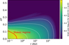 |
Fig. 7 Grain size for which the local Stokes number is equal to 10−3, as a function of position in the const background disk model. The red curve encloses where particles of the size for which St = 10−3 are in the Stokes drag regime. |
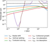 |
Fig. 8 Behaviour of the timescales associated with various disk processes as a function of radial distance r. Timescales shown are for a monomer of size sm = 10−5 m with a pure H2O ice mantle, located at z/r = 0.05. The dashed line at t = 108 yr indicates the upper limit on timescales relevant for planet formation. |
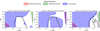 |
Fig. 9 Process coupling behaviour for different grain sizes and ice mantle compositions. Colored areas indicate the decoupling of the different timescale groups. The filling of the coloured areas with solid lines or dots indicate the decoupling of a process category since it is much faster or slower, respectively. Black lines indicate icelines (τads = τdes). |
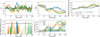 |
Fig. 10 Evolution of the vertical positions (upper left panel), radial positions (upper center panel), temperatures (upper right panel), local UV fluxes (lower left), and local molecular number density in the gas phase (lower center) for monomers in home aggregates with different fragmentation velocity υfrag, released from r = 10 AU and z/r = 0. The black dashed line in the lower left panel indicates a UV radiation field strength of 1 FDraine. Linestyles in the lower center panel indicate number densities of different gas phase species. |
3.2 Model demonstration and effects of different fragmentation velocity
As a first demonstration of the full SHAMPOO code, we consider the evolution of three monomers, initially not embedded in a home aggregate. The monomers are allowed to be incorporated in aggregates which have a fragmentation velocity of υfrag = 1, 5, or 10 m s−1. For each of these three scenarios, the appropriate background disk model is used (vFrag1, vFrag5, and vFrag10, respectively), while the monomers are released from z = 0 at r = 10 AU. The initial ice budget of the monomers is informed from the respective background disk model via Eq. (71). This means that the monomers start with a total amount of ice of mice = 0.0174mm, 0.0176mm, and 0.0113mm in the vFrag1-, vFrag5-, and vFrag10-model, respectively. The three monomers are allowed to be processed for 105 yr. All home aggregates are assumed to have a filling factor of ϕ = 0.1 for all three scenarios. However, in practice the filling factor can differ for each home aggregate. We therefore explore the effects of different filling factors in Sect. 3.3. The random number generator seed is kept fixed between all three scenarios, such that the fragmentation velocity and the associated background disk model are the only differences between the three simulations.
3.2.1 Dynamical and environmental evolution
Figure 10 shows the evolution of the vertical and radial position of the monomer, the associated monomer temperature and local UV radiation field. The monomer temperature is assumed to be equal to the local dust temperature. Despite the same initial monomer properties and model seed, the three monomers follow clearly distinct dynamical trajectories within the first 10 kyr.
It becomes clear that all monomers are in the dynamical regime dominated by turbulent diffusion (Fig. 7). In the vertical dimension, Fig. 10 shows that in all three cases the monomer makes several vertical excursions to |z/r| ~ 0.2, whereas radially, all three monomers diffuse significantly inwards, with all monomers reaching inside of r = 6 AU in 100 kyr. As the monomers gradually diffuse inwards, all three monomers experience increasing temperatures. However, the monomer in the vFrag1 -model remains cooler than the other monomers between 60 and 80 kyr as it remains around r = 8 AU in this period, while the monomers in the vFrag5 - and vFrag10-model have already diffused interior to r = 6 AU after 60 kyr. We also discern small peaks in the temperature evolutions of the monomers, which can be associated in time with the short-lived vertical excursions.
Figure 10 also reveals that the local UV radiation field strength is usually below 1 FDraine for all three monomers, although exceptions are short peaks in field strength, which can be again attributed to vertical excursions higher in the disk atmosphere. The monomer in the vFragl-model here experiences significantly less peaks in field strength compared to the vFrag5- and vFrag10-model. These latter background models have a thinner dark midplane region (Figs. A.2–A.4), and thus smaller vertical excursions are necessary for a monomer to reach the irradiated surface disk layers. Altogether monomers in the vFrag5- and vFrag10-model are more often in a regime where photodesorption can remove ice. The highest peaks in UV radiation field strength are found between 25 and 30 kyr for the monomer in the vFrag5-model and 40 and 25 kyr for the monomer in the vFragl-model, where the UV radiation field very briefly peaks at 102FDraine on both occasions. Although there exist many other peaks in UV radiation field strength, these peaks are usually well below 1 FDraine and of short duration. Altogether we thus expect photodesorption to affect the ice evolution of monomers only for short periods of time if a monomer is exposed during a peak in the background UV radiation field.
3.2.2 Collisional history
The collisional histories of the three monomers are shown in Fig. 11, where we consider the evolution of the home aggregate size. Figure 11 also shows the type of interactions which result in a change in home aggregate sizes. We also count the number of collision outcomes per monomer history, giving rise to Table 4.
Figure 11 and Table 4 show that fewer collisions occur over 100 kyr for increasing υfrag. The monomer in the vFrag10-model undergoes less than half as many collisions as the monomer in the vFrag1-model (530 collisions compared to 1165). This is a consequence of the total dust surface mass density Σd in the background disk model. In the background disk models with higher υfrag, larger dust aggregates can form (see also Fig. 2), and thus the same amount of dust mass becomes concentrated in fewer dust particles, which in turn lowers collision rates. This is also confirmed by the typical home aggregate size seen in Fig. 11: sa can be larger than 1 cm in the vFrag 10-model, while it is smaller than 1 mm in the vFrag1-model. We note that these home aggregate sizes are expected based on the maximum grain sizes allowed between r = 4 AU and r = 10 AU according to Fig. 2. Furthermore, for all three models, the frequency of collisions increases later in the evolution, which is a consequence of the radial diffusion inwards towards higher density disk regions (Fig. 10) for all three monomers.
Although there are thus significant differences between the collision histories of the three monomers, coagulation is the most frequent collision outcome for all three fragmentation velocities, amounting to almost 90% of the collision outcomes in all three cases. Aggregate fragmentation and erosion (comprising erosion, ejection, and impact events) appear to be rather rare compared to coagulation, in particular for the vFrag 5- and vFrag10-model. However, we note that coagulation is the only event allowed for collisions with υrel < υfrag, which is true for most collisions in the monomer history. Once the home aggregate has grown to a size at which collisions with υrel > υfrag become commonplace, destructive collisions usually result in a smaller home aggregate, placing it back in the regime where, υrel < υfrag·
Figure 11 shows that the largest decreases in home aggregate size are associated with monomer ejection, undoing the work of many coagulation events. This is expected since in these events, the monomer we track ends up in a fragment produced by erosion of the previous home aggregate. These fragments are guaranteed to be significantly smaller than the previous home aggregate (Sect. 2.3).
Although coagulation can produce large sudden increases in home aggregate sizes (e.g. the first 5 kyr in the vFrag 10-model), we also discern many episodes in all three models where the home aggregate grows through the sweep-up of many smaller aggregates. We note that the behaviour exhibited in Fig. 11 is similar to the aggregate size history shown as an example in Krijt & Ciesla (2016).
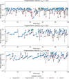 |
Fig. 11 Collision histories and resulting home aggregate sizes sa as a function of time for monomers in aggregates of different fragmentation velocities υfrag. Note that the vertical position of each collision event coincides with the home aggregate size sa after the collision has occurred. |
 |
Fig. 12 Evolution of monomer depth zm for monomers embedded in home aggregates with υfrag = 1 m s−4 (left), 5 m s−1 (center), and 10 m s−1 (right). Green areas denote the times at which the monomer is exposed to gas phase molecules and UV photons, while the monomer is shielded from impinging molecules and UV photons otherwise. In each panel, the dashed line indicates zm = zcrit. |
 |
Fig. 13 Evolution of the total ice mass mice of monomers in aggregates with different fragmentation velocity υfrag (left panel), together with snapshots of the monomer ice composition at 10 kyr (center panel), and 100 kyr (right panel). |
3.2.3 Ice evolution
The evolution of the amount of ice on monomers depends on the local abundances of gas phase molecules at a given time (lower center panel of Fig. 10). Furthermore, the evolution of the monomer ice mantle crucially depends on the depth at which the monomer is embedded in its home aggregate zm, which is depicted for the three scenarios in Fig. 12. The monomer depth, which is a product of the collisional history, in combination with dynamical processes gives rise to the ice evolution depicted in Fig. 13. Since aggregates with lower fragmentation velocity remain smaller, it is more likely that the monomer is located close to the surface. Therefore, we find in Fig. 12 that the monomer in the vFrag1-model has the lowest average monomer depth compared to the vFrag5- and vFrag10-models. As a consequence, the monomer in this model is also exposed to the gas phase most often. In the vFrag10-model, the monomer only experiences one short initial period of exposure, which is mainly a result of our initial condition for the monomer to start without a home aggregate. For most of its evolution, the monomer in the vFrag10-model is located below zm = 10−4 m. The vFrag5-model represents the intermediate case where the episodes of exposure after the initial phase occur less frequently than for the monomer in the vFragl-model.
Figure 13 shows the evolution of the total amount of ice on the three monomers, along with snapshots of the monomer composition at 10 kyr and 100 kyr. Although the monomer in the vFrag1-model is exposed to gas phase molecules most often, the left panel of Fig. 13 shows that after 100 kyr, the monomer has a similar total amount of ice (2.1 × 10⁻³mm) as the monomer in the vFrag10-model (1.8 × 10⁻³mm). Both models lost significant amounts of ice. In the vFrag1-model, this is the consequence of the monomer being exposed around 40 kyr, where the monomer makes a significant vertical excursion (Figs. 10 and 12), allowing all ice to evaporate in the strong UV radiation field via photodesorption. However, the frequent episodes of exposure do allow the monomer to regain a small amount of ice after the photodesorption around 40 kyr.
Although the monomer in the vFrag10-model is protected from photodesorption – as it is almost always unexposed, the left panel of Fig. 13 shows that it still loses a significant amount of ice between 70 kyr and 80 kyr; a period where it also experiences the highest temperatures (~90 K) of all three monomers. Moreover, the snapshot of ice composition at 100 kyr in the right panel of Fig. 13 shows that the monomer in the vFrag10-model has lost all its H2O ice, while at 10 kyr, all three monomers have similar amounts of water (center panel of Fig. 13). This is striking since the H2O iceline based on the adsorption and desorption timescales is located around r ≈ 2 AU around the disk midplane for all background models, a radial distance which is not reached by any of the monomers. Therefore, the adsorption rate is larger than the thermal desorption rate. However, since the monomer in the vFrag10-model is always unexposed, all the impinging molecules are adsorbed by monomers closer to the home aggregate surface. As the monomer we track is shielded from adsorption in this case, thermal desorption causes this monomer to lose all H2O ice on its surface, despite the aggregate being located behind the H2O ice line. However, this may be an overestimate of the amount of H2O lost, as the H2O lost through thermal desorption may in reality be partially replenished by the re-adsorption of H2O originating from other nearby monomers (see also Appendix B).
Compared to the other two monomers, the evolutionary trajectory for the monomer in the vFrag5-model is less dramatic, with more moderate episodes of adsorption during exposure and desorption at 20 and 90 kyr. We note that this monomer is unexposed at the times of ice loss, suggesting that this loss occurs in a similar although less extreme fashion as for the vFrag10-model.
In terms of composition, the center and right panel of Fig. 13 show that at 10 kyr, the three monomers have ice mantles of similar composition. Here, H2O is the dominant ice species with smaller amounts of NH3 and CO2. It becomes clear that in addition to the H2O ice loss for the monomers in the vFrag1- and vFrag10-model, all three monomers have lost their CO2 after 100 kyr. This is a result of the low adsorption energy of CO2 compared to H2O and NH3 ( K compared to
  K and
K and  K; McElroy et al. 2013). As all three monomers gradually diffuse inwards towards warmer disk regions, we expect all CO2 to be lost through thermal desorption. On the contrary, the amount of NH3 after 100 kyr remains fairly constant for all three monomers. For the monomer in the vFrag5- and vFrag10-model, this can be explained through the high adsorption energy of NH3, which means that the role of thermal desorption is limited in comparison to CO2 and H2O. We note that lower values for Eads,NH3 have been inferred (e.g. Sandford & Allamandola 1993; Brown & Bolina 2007), which would result in NH3 being less stable against thermal desorption in this disk region. For the vFrag1-model, all NH3 ice at 100 kyr must have accumulated after the photodesorption event at 40 kyr, indicating that significant NH3 adsorption has occurred after this catastrophic ice loss.
 |
Fig. 14 Evolution of the total amount of ice (left panel), H2O ice (center), and NH3 (right) averaged over 500 monomers for different home aggregate filling factors. Solid lines indicate the mean of the 500 monomers, whereas dotted lines indicate the standard deviation. The black dots indicate the ice evolution behaviour predicted by ProDiMo for the vFrag5-model. Trajectories of individual monomers are also shown in the background. |
3.3 Comparison to background model and effects of filling factor
Throughout this work, the home aggregates were assumed to have a filling factor of ϕ = 0.1 or ϕ = 1, which is consistent with dust aggregates which have undergone some degree of compaction. Experiments have demonstrated that typical filling factors ϕ associated with compact aggregates range from ϕ ~ 0.2 (Langkowski et al. 2008) up to ϕ ≂ 0.4 (Weidling et al. 2009, 2012). Alternatively, modelling work has shown that large, fluffy aggregates with ϕ ≲ 10−3 can form if sticking is efficient and fragmentation is inefficient (Okuzumi et al. 2012; Kataoka et al. 2013). Since the value of ϕ affects how often a monomer is exposed and can accumulate ice, it is key to explore the sensitivity of ice formation in our model on ϕ. Furthermore, ice evolution is also considered in the time-dependent chemistry of the ProDiMo background models. Therefore, we can compare the ice evolution predicted for a local monomer population by SHAMPOO to the ice evolution calculated by ProDiMo.
For these purposes, we consider the evolution of the average amount of ice present on 500 monomers over 100 kyr in the vFrag5-model in Fig. 14. Four different scenarios are considered in Fig 14, where monomers are embedded in home aggregates with a constant filling factor of ϕ = 1, 10−1, 10−2 or 10−3. As we also aim to compare the results to the fully local evolution predicted by the time-dependent chemistry in ProDiMo over the same time period, the monomer positions are fixed at r = 10 AU in the disk midplane. This also means that the local disk environment remains the same for all simulations. Tests with dynamical processing enabled were also performed and yielded qualitatively similar results for the total amount of ice as shown in this section. However, the inclusion of dynamics results in a significant increase in the diversity of monomer trajectory and hence the standard deviation.
Initially, all monomers are assigned to a home aggregate of random size sa which is drawn from the background model dust mass distribution ρd(a, r, z). Subsequently the monomer depth zm is drawn from a spherically uniform probability distribution, such that the initial values of both sa and zm are weighted with the distribution of dust mass in the background model. All monomers start with 0.0176 times their bare monomer mass mm worth of ice, which is calculated according to Eq. (71). The left panel of Fig. 14 shows that for all values of the home aggregate filling factor ϕ, monomers gain ice over the 100 kyr evolution, primarily as a consequence of the adsorption of H2O and to a lesser extent, NH3 and CO2. The amount of ice accumulated, however, depends on the filling factor ϕ. Fig. 14 shows an increase of the total amount of ice of only 0.93% for monomers in aggregates with ϕ = 1, while monomers in very porous aggregates with ϕ = 10−3 on average gain ~20% their initial ice mass worth of ices over 100 kyr. The intermediate cases of ϕ = 10−2 and ϕ = 10−1 result in an average increase in the total ice mass of 6.1 and 2.0%. This decrease in the efficiency of ice adsorption for increasing ϕ is a result from the lower exposure probability Pexp at given zm for higher filling factors. Figure 5 shows that for ϕ = 10−3, 10−2, 10−1, and 1, gas phase molecules can respectively reach down to depths of approximately 2 × 10⁻⁴ m, 2 × 10⁻⁵ m, 2 × 10⁻⁶ m, and 2 × 10⁻⁷ m. Therefore, monomers spending time in aggregates with higher ϕ spend less time exposed to the gas phase.
The center and right panels of Fig. 14 show that most of the ice accumulated during the 100 kyr evolution is H2O and NH3 for all values of ϕ. In all cases, these two species amount to over 90% of the molecules gained as ice, with the remainder being CO2. This is a result from the fact that H2O and NH3 are the most prevalent molecules at 10 AU in the gas phase of our background model, with molecule number densities of  and
and  (Appendix A.2). Although CO and CH4 are much more abundant in the gas phase (nCO ≈ 2.4 × 10¹⁴ m−3 and
  ), these molecules do not form any ices since temperatures at 10 AU are too high (see also Fig. 9).
Figure 14 also shows the average amount of ice expected on monomers based on the ice evolution predicted by the time-dependent chemistry of the vFrag5 ProDiMo model. We linearly interpolate between the default snapshot for nx,ice at t = 2 × 10⁵ yr used in the background model and a new snapshot at t = 3 × 10⁵ yr obtained by evolving the chemistry in the vFrag5 ProDiMo model. The molecule number densities nx,ice calculated in ProDiMo are here converted to units of ice mass per monomer with Eq. (71), which results in an increase of the total amount of ice of only 0.89% in the background model. This is roughly 10% less than the average total amount of ice expected on monomers in aggregates with ϕ = 1. We also find that in the cases of specific species, the average amount of H2O and NH3 on monomers in aggregates of ϕ = 1 calculated with SHAMPOO is ~10% above the increase calculated by ProDiMo. It is expected that monomers in aggregates with ϕ = 1 are in best agreement with ProDiMo, as ProDiMo chemically treats the refractory component of individual dust particles as rigid balls where molecules do not penetrate the aggregate surface upon adsorption. In ProDiMo, ice will only build up in a homogeneous layer on the aggregate surface, such that the rate at which ice of species x is adsorbed on a single dust aggregate is given by

In SHAMPOO, the effective adsorption rate for the same aggregate can be estimated as

with Nexp being the total number of exposed monomers in the aggregate. In practice, this means that a given aggregate has on average more surface area available for adsorption than a dust particle of the same size in ProDiMo, since monomers below the aggregate surface can have have nonzero exposure probability, allowing for very large Nexp if the filling factor is low. Even for ϕ = 1, Fig. 5 shows that molecules can reach a few monomer radii below the aggregate surface, although the exposure probability drops off very quickly. This nonzero exposure probability down to a few monomer radii overestimates the surface area available for adsorption with respect to ProDiMo, and thus explains ~10% difference.
4 Discussion
4.1 Applications
The SHAMPOO code provides a tool which allows the investigation of the systematic behaviour of dust monomers under the non-local disk processing of a given protoplanetary disk structure. In this section we highlight a number of possible applications of the SHAMPOO code.
The primary goal of SHAMPOO is to reliably predict the CHNOS abundances of dust during the first stages of planet formation, where no planetesimals have formed yet. In case of the Solar System, this would encompass the first 100–500 kyr after the formation CAIs (e.g. Kruijer et al. 2014, 2020). In order to infer local CHNOS abundances in local dust populations, many monomer trajectories would be required. Within the framework of the background disk model, each monomer can be assigned to one spatial grid cells of the background disk model. This means that at any moment in time, every monomer is representing a unit of mass from that spatial grid cell. Predictions for the local CHNOS abundances can then be made by averaging over the individual CHNOS abundances of the monomers associated with that grid cell. A crucial requirement is that the spatial grid resolution is high enough such that the physical, thermal and chemical gradients within a grid cell are small.
Although this work has primarily focussed on the CHNOS-bearing molecules condensed on the monomer as ices, every monomer also consists of a refractory component of mass mm. This refractory component can also contain a significant fraction of the total CHNOS elemental budget (e.g. Öberg & Bergin 2021). Currently, SHAMPOO does not assign a specific composition to the refractory component, although this could be incorporated in the model for example by assigning a static composition to the refractory monomer component. This refractory composition can be informed from the conditions at which the refractory component of the monomer has condensed. Altogether this would allow for a complete picture of the evolution of local CHNOS abundances.
We note a number of possible applications of SHAMPOO outside its main application. Specifically, SHAMPOO could be used to study the effect of dynamical and collisional processes on the transport of physically or chemically altered minerals throughout the planet-forming disk. Examples here include the possible outward diffusion of processed refractory material such as crystalline sillicates (e.g. Bockelée-Morvan et al. 2002; Watson et al. 2009; Olofsson et al. 2009; Williams et al. 2020), and the transport of hydrated minerals throughout the planet-forming disk (e.g. Brearley 2006; D’Angelo et al. 2019). However, such an application would involve connecting SHAMPOO to models which describe how these processes alter a single monomer given a certain disk environment. Another application lies in predicting the composition of pebble fluxes over time (e.g. Lambrechts & Johansen 2014; Morbidelli et al. 2015). The growth of pebbles involves the compaction of aggregates (i.e. ϕ increases over time) which gradually lowers the sticking probability after a collision. Therefore, such a compact aggregate would ultimately collisionally decouple from the growth-fragmentation cycles shown in Fig. 11 due to the bouncing barrier (Güttler et al. 2010; Zsom et al. 2010; Krijt et al. 2018). The application of SHAMPOO in this context would thus require the inclusion of porosity evolution. Furthermore, an application of SHAMPOO could lie in tracking the effects of non-local disk processing on local isotopic ratios such as D/H, 13C/12C, 15N/14N, and 18O/16O (see e.g. Cleeves et al. 2014; Visser et al. 2018; Öberg & Bergin 2021). This would, however, require the incorporation of the isotopologues in the background model chemical network and possibly also the feedback of sublimation into the background gas phase composition.
4.2 Model limitations
In this section we discuss the fundamental limitations of the SHAMPOO code, and highlight how we expect that these limitations are likely to affect predictions made with the SHAMPOO code both in this work and future work.
4.2.1 Feedback of monomer evolution on the disk
The code presented in this work offers a comprehensive description of how disk processes affect the volatile CHNOS abundances of monomer particles. However, the local conditions which affect the monomers are completely set by the background model, and are independent of the evolutionary trajectories of monomers. We highlight a number of effects this assumption may have on the evolutionary trajectories predicted by SHAMPOO.
In Fig. 4 we highlighted the possibility of inconsistencies between the local dust size distribution ρd(a, r, z) in the background disk model (Eq. (5)) and the in-situ dust size distribution inferred from the residence time of the monomer in home aggregates of given size. However, these two distributions are not independent since the background dust size distribution determines the collision rates (Eq. (22)). In Fig. 4 we demonstrated that given enough time, the time spent by the monomer in a home aggregate of given size approximately follows the residence time one would expect from the background distribution. However, we also noted significant departures, in particular when the dust size distribution of the background model is not consistent with the steady-state dust size distribution associated with a given fragmentation velocity υfrag in the collision model (Sect. 2.3). In the background model dust size distribution, the maximum size is specified directly by amax, whereas in the collision model, the maximum home aggregate size also depends on the fragmentation velocity υfrag. In reality, however, amax is a function of the fragmentation velocity. In this work, we accounted for inconsistencies between the maximum aggregate size in the collision model and amax by using the parametrization from Birnstiel et al. (2012) for a local, steady-state distribution if turbulence is the main source of relative velocity between dust particles. However, amax does remain a quantity which is not calculated self-consistently and has to be estimated separately from the SHAMPOO-code in the background model.
As a consequence of this discrepancy between the imposed background distribution and the steady-state distribution expected from the collision model, we found in Fig. 11 that monomers in aggregates with too low fragmentation velocity in SHAMPOO (i.e. the background model contains too many large grains) are frequently forced into aggregates which are larger than possible given the value of υfrag. In these larger aggregates, monomers are more likely to be buried at larger monomer depth zm, which results in a lower exposure probability. Similarly, a too high fragmentation velocity in SHAMPOO (i.e. the background model does not contain enough large grains) results in monomers spending much time in large aggregates which are not present as grains in the background model. This would thus also result in an underestimation of the exposure probability. For the volatile CHNOS budgets, this means that inconsistencies between the background model and the collision model will likely result in our model underestimating the effects of adsorption and photodesorption on the ice budgets of monomers. The results of Sect. 3.2 show that in particular photodesorption can have extreme effects on the evolution of monomers which are exposed frequently. Inconsistencies between the collision model and the background model would thus underestimate these effects, which highlights the importance of keeping the grain size distribution implied by the collision model and the grain size distribution of the background disk model as consistent as possible.
In our background disk model, we allow for the condensation and sublimation of molecules onto monomers. Since the position of the monomer between the time of condensation and sublimation of a particular molecular changes, the gas phase abundance of the molecule can become depleted in disk regions of systematic condensation onto monomers, and enriched in regions of systematic sublimation. SHAMPOO predicts the effects of a given chemical disk structure on the evolution of individual dust particles. However, it does not incorporate the effects of systematic behaviour of monomers on the disk chemical structure. It is expected that this systematic behaviour does affect the disk chemical structure on ~1 Myr timescales (e.g. Zhang et al. 2020; Krijt et al. 2020), which may in turn affect monomers which are processed in the same region at later times. In future work, we aim to quantify the initial net gas phase depletion-and enrichment fluxes at a certain disk region using the systematic behaviour of many monomers that visit that region. This approach would enable us to constrain the timescales where the condensation or sublimation of volatile molecules have large effects on local gas phase abundances. Altogether it becomes clear that predictions of monomer trajectories made with SHAMPOO are not reliable on timescales comparable to ~1 Myr due to the expected chemical feedback on the gas phase. However, other evolutionary processes such as disk evolution and planet formation are also expected to undermine the assumption of a static background disk environment on these timescales (e.g. Andrews 2020; Raymond & Morbidelli 2022). As a precaution, we have therefore chosen a timescale (100 kyr) significantly shorter than 1 Myr as the upper bound for the simulation time for individual monomers throughout this work.
4.2.2 Optical depth formalism
In Sect. 2.4 we introduced a new stochastic approach for estimating ice adsorption and photodesorption for a monomer embedded at a certain depth zm inside its home aggregate. In this approach, we assumed the monomer to be buried at a depth zm below a homogeneous slab of monomers associated with an “optical depth” τ. However, the expression for τ derived in Eq. (51) strictly applies to aggregates of constant density (i.e. nm does not vary as a function of time or position in the aggregate). In reality, however, nm does vary as a function of position in the home aggregate and evolves over time due to collisional processing.
The most notable effect here is compaction (Weidling et al. 2009; Güttler et al. 2010; Zsom et al. 2010). This is a process which is not explicitly modeled in this work, although the assumed filling factor of ϕ = 0.1 is consistent with aggregates which have undergone some degree of compaction (e.g. Langkowski et al. 2008; Weidling et al. 2009). The fact that nm depends on position in the aggregate and changes over time due to collisions has important effects on the exposure probability Pexp and the new monomer depth zm after a collision. The results in Sect. 3.3 suggest that accumulation of new ice is more efficient in porous aggregates, and thus gradual compaction implies that ice formation is a process that becomes more and more confined towards the aggregate surface at later times.
Another simplification made is that the optical depth τ associated with a certain monomer depth zm is assumed to be the same for impinging gas phase molecules and UV photons. In practice however, UV photons will likely be able to penetrate deeper into the aggregate since the minimum wavelength of UV photons (≳10−8 m) is either comparable or larger than the monomer size (sm = 5 × 10⁻⁸). This would imply that the exposure probability for photodesorption at a given depth would be larger, and hence more monomers would be able to lose ice via photodesorption. For r ≂ 10 AU, the results from Sect. 3.2 suggest that the effects of photodesorption are significant for individual monomers in smaller, more fragile aggregates (υfrag = 1 m s−1) in that disk region, even with no distinction between the optical depth for photons and molecules. For these monomers, our current model may thus underestimate the average amount of ice lost due to photodesorption. Similarly, a lower filling factor also reduces the optical depth, and thus is more likely to leave monomers exposed to impinging UV photons. As a function of position, Figs. A.1–A.4 show that for larger radial distances (r ≳ 100 AU), UV photons can reach deeper in the disk. Therefore, our model may also underestimate the amount of ice lost via photodesorption in small, fragile aggregates at large radial distances. However, the examples in Sect. 3.2 do suggest that the effect of photodesorption is less important for monomers residing in aggregates with higher υfrag, as the monomer is on average located at considerably larger zm in these aggregates (Fig. 12). Therefore, we expect that the effect of a distinction between the optical depth for molecules and UV photons will remain limited for monomers in aggregates with higher υfrag.
5 Conclusions
In this work we introduced and benchmarked the SHAMPOO code, which models the effects of dynamical, collisional and ice processes on the volatile CHNOS abundances of individual dust particles. In addition, we also motivated the need for this model, and used the SHAMPOO code to investigate the effects of different fragmentation velocities and aggregate filling factor on ice evolution at 10 AU. We summarize our conclusions as follows:
The dynamical behaviour of a dust grain of given size can vary greatly as a function of position throughout the disk. This is a consequence of the fact that the grain size associated with the Stokes number for which aerodynamic drag starts to significantly affect the grain dynamics (St = 10−3) varies greatly throughout the disk (Fig. 7). This is primarily a result from the large variation of the gas density throughout the disk, and to a lesser extent also from the gas temperature.
The disk regions where the timescales associated with dynamical, collisional, and ice processing couple varies, depending on grain size and ice species (Fig. 9). However, different grain sizes are connected through collisional processes, and the ice mantle of a dust particle can consist of multiple ice species. Therefore, we require a fully coupled modeling approach such as SHAMPOO to make physical estimates of the volatile CHNOS during the first stages of planetesimal formation.
For a fragmentation velocity of υfrag = 1 m s−1, the monomer spends more time in smaller aggregates, and is therefore on average located closer to the aggregate surface (Figs. 10–13). A lower monomer depth increases the exposure probability Pexp, resulting in more periods of monomer exposure to the gas phase compared to monomers in aggregates of higher υfrag. On the one hand this means that monomers in fragile aggregates can more frequently accumulate ice through adsorption. On the other hand, the exposure to the gas phase can also result in enhanced ice loss through photodesorption if the period of exposure coincides with a large vertical excursion of the monomer to the disk surface. Altogether, our results suggest that the interiors of fragile aggregates are more likely to have undergone extensive ice processing than aggregates with a higher fragmentation velocity (υfrag = 5, 10 m s−1).
In the absence of dynamical transport, the average ice budgets of aggregates with ϕ = 1 are in good agreement with the ice abundance predicted by the time-dependent chemistry of the ProDiMo background disk model. Furthermore, very porous aggregates (ϕ = 10−3) have a higher exposure probability Pexp at a given depth. Therefore, gas phase molecules can reach deeper into these aggregates, and these aggregates accumulate more ice (Fig. 14). As a consequence, the ice mantles of monomers inside these aggregates are likely more processed compared to monomers inside more compact aggregates.
Altogether SHAMPOO provides a useful tool for probing the dust processing on a microscopic level. In future work, we aim to use a large set of its individual dust grain simulations to study the influence of non-local disk processing on local CHNOS abundances. Although the model has been developed to study the processing of CHNOS, we also noted applications of SHAMPOO outside its main purpose. Examples included the formation and transport of physically or chemically processed material, such as crystalized sillicates or hydrated minerals, and the formation and evolution of pebbles.
Acknowledgements
The authors would like to thank Rens Waters and Kaustubh Hakim for comments and insightful discussions, and an anonymous reviewer for constructive comments that helped to improve our simulations. This work is part of the second round of the Planetary and Exoplanetary Science Network (PEPSci-2), funded by the Netherlands Organization for Scientific Research (NWO).
Throughout this work, particle “size” signifies the (effective) radius of a dust particle.
Official webpage: https://prodimo.iwf.oeaw.ac.at/
Throughout this discussion, the usage “grain” signifies a dust particle which is either part of the background model or a collision partner, whereas “aggregate” refers to dust particles containing a monomer.
Appendix A Structure and composition of the background disk models
The physical disk structure of the const, vFrag1, vFrag5 and vFrag10 background models is shown in Sect. A.1 while Sect. A.2 presents the chemical structures.
Appendix A.1 Physical background disk structures
Overview of the spatial structures of gas temperature Tg, dust temperature Td, gas mass density ρg, dust mass density ρd and UV radiation field strength χRT provided by the background disk models.
 |
Fig. A.1 Physical disk structure of the const-model. |
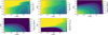 |
Fig. A.2 Physical disk structure of the vFrag1-model. |
 |
Fig. A.3 Physical disk structure of the vFrag5-model. |
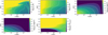 |
Fig. A.4 Physical disk structure of the vFrag10-model. |
Appendix A.2 Chemical background disk structure
Overview of the gas (left columns) and ice (right columns) number densities (nx) of various molecules provided by the background disk models in m−3. In each figure from top to bottom: H2O, NH3, CO, CO2, CH4 and H2S.
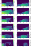 |
Fig. A.5 Chemical disk structure of the const-model. |
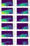 |
Fig. A.6 Chemical disk structure of the vFrag1-model. |
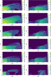 |
Fig. A.7 Chemical disk structure of the vFrag5-model. |
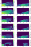 |
Fig. A.8 Chemical disk structure of the vFrag10-model. |
Appendix B Diffusion timescales inside the home aggregate
In our treatment of desorption in Sect. 2.4, molecules originating from monomers deep inside aggregates are assumed to escape the aggregate instantaneously. However, this assumption may be inappropriate for significant filling factors, as the mean free path for a molecule traveling inside an aggregate is usually shorter than sa, which means that molecules liberated by desorption will undergo collisions with other monomers in an aggregate before escaping to the gas phase. This may result in re-adsorption, allowing to possibly retain more ice in the unexposed aggregate interiors than accounted for in the current model. Similarly, this mechanism could also provide a pathway for freshly accumulated ice molecules on exposed monomers to diffuse towards the unexposed monomers deeper in the aggregate. In this section, we develop a simple model to constrain the importance of this process by defining and estimating an upper bound of the timescale associated with the escape of molecules from the aggregate.
We assume that the liberated molecules effectively undergo a random walk as collisions with other monomers occur while escaping the aggregate. If liberated molecules only collide with monomers, the escape timescale τesc associated with a molecule depends on two main factors: the number of random walk collisions between the molecule and other monomers nc before the molecule escapes the aggregate, and the fraction of these collisions which results in re-adsorption, which is given by the sticking factor S (Eq. (57)). Altogether we can thus express τesc as
 (B.1)
(B.1)
Here, τmc denotes the molecule collision timescale, and can be expressed as
 (B.2)
(B.2)
 in this case denotes the mean free path inside the aggregate. We here use the monomer density nm as given in Eq. (50). ν denotes the velocity of the molecule while it travels between monomers. Since we aim to obtain an upper bound on the escape timescale, we estimate ν with the molecule ice diffusion speed, which we estimate from the thermal hopping timescale τhop (i.e. the average time for a molecule to migrate from one site in the ice lattice to the next) (e.g. Thi 2015; Ruaud et al. 2016; Cuppen et al. 2017),
 (B.3)
(B.3)
Here, ds ≃ 10−10 m (e.g. Caselli & Ceccarelli 2012) denotes the average distance between two molecule binding sites in the ice lattice. vx is the lattice vibration frequency as given by Eq. (59) and Edilff,x denotes the diffusion energy, which we estimate as  Similarly, the desorption timescale for a single molecule τd (in addition to the ice mantle desorption timescale τdes defined in Eq. (73)) for molecule species χ can be expressed as (e.g. Thi 2015)
 (B.4)
(B.4)
Altogether we write Eq. (B.1) as
![Mathematical equation: ${\tau _{{\rm{esc}}}} = {{{n_c}} \over {{v_x}}}\left[ {{{4{s_m}} \over {3\phi {d_s}}}{\rm{exp}}\,\left( {{{{E_{{\rm{ads,}}x}}} \over {2{k_{\rm{B}}}{T_{\rm{d}}}}}} \right) + S\,\exp \,\left( {{{{E_{{\rm{ads,}}x}}} \over {{k_{\rm{B}}}{T_{\rm{d}}}}}} \right)} \right].$](/articles/aa/full_html/2023/06/aa45537-22/aa45537-22-eq107.png) (B.5)
(B.5)
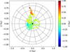 |
Fig. B.1 Example of a 3D random walk through an aggregate of radius sa = 10−5 m and ϕ = 0.5 (top view). The colorscale indicates the z-coordinate of the molecule. The black dot and cross denote the starting point and the location where the molecule crosses the aggregate surface, respectively. |
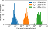 |
Fig. B.2 Distribution of escape timescales of 100 model runs in aggregates of ϕ = 0.5 and varying radius. Molecules are always released from the center of the aggregate. |
It becomes clear from Eq. (B.5) that τesc is very sensitive to Td. On the one hand, this will result in extremely long τesc for aggregates significantly inside the ice-forming region, as thermal desorption becomes a very slow process (see also Sect. 3.1), resulting in extremely long τd. Furthermore, S ≃ 1 in these regions, which means that even if a molecule undergoes thermal desorption, it will be re-adsorbed almost instantaneously by another nearby monomer. On the other hand in warm regions where τd becomes very short and S → 0, we also expect that re-adsorption will not have a significant effect on monomer ice mantle composition, as τesc will be dominated by the molecule collision timescale τmc. Altogether Eq. (B.5) suggests that the effects of re-adsorption of species x on monomer ice mantle composition are the largest near the iceline associated with species x. However, another crucial factor in determining the value of τesc is the number of collisions before escape nc, which depends on aggregate size sa and filling factor ϕ.
In order to constrain nc and provide an upper bound on τesc near the iceline, we consider a simple numerical 3D spherical random walk model. In this random walk model, individual molecules move from one position to the next in steps of size λmfp in a spherically random uniform direction. The simulation ends when the molecule distance to the aggregate center is larger than the aggregate radius (i.e.  ). This gives rise to trajectories of individual molecules through the aggregate. An example of such a trajectory is shown in Fig. B.1, where a molecule is released from the center of an aggregate with sa = 10−5 m and ϕ = 0.5, and undergoes nc = 7124 collisions before escaping the aggregate. Altogether individual molecules can take significant detours through the aggregate, resulting in a considerable variation in nc and τesc associated with the trajectories of individual molecules. Therefore it is necessary to evaluate Eq. (B.5) for a larger set of molecules.
As a next step therefore we consider the distribution of τesc for 100 H2O molecules escaping from the center of aggregates of sa = 10−6, 10−5, and 10−4 m at the H2O iceline (Td ≈ 140 K, c.f. Fig A.1 and Fig. A.5). As we expect that the effects of readsorption are most important for larger aggregates with a short mean free path, we consider a filling factor ϕ = 0.5. The direct dependence of τesc on ϕ in Eq. (B.5) suggests that larger ϕ results in shorter τesc. However, a shorter mean free path will also result in larger nc, which effectively results in the escape timescale being longer for higher ϕ. The resulting escape timescales distributions τesc for the different aggregate sizes are shown in Fig. B.2. Molecules escape faster from smaller aggregates due to the lower average number of collisions nc before escape. Fig. B.2 reveals that the average value of τesc increases orders of magnitude per order of magnitude increase in sm. This suggests that for aggregates larger than 10−4 m (i.e. millimetre- and centimetre-sized aggregates), the escape timescale may become comparable to the timescales of other disk processes (c.f. Fig. 8). Since the largest aggregates contain most of the dust mass (c.f. Fig. 4), Fig. B.2 implies that re-adsorption after thermal desorption in unexposed aggregate interiors may have significant effects on the average amount of ice retained in monomer ice mantles. Specifically, our model could overestimate the amount of ice lost via thermal desorption on unexposed monomers. However, an increase or decrease of 10 K from Td was also found to result in a decrease or increase in τesc of almost 2 orders of magnitude, respectively. This suggests that the disk region where τesc couples to the other disk processes is spatially limited to a small region just behind the H2O iceline. However, this also means that there always is a region where τesc couples to the other disk processes, and thus can affect ice composition on timescales similar as the other disk processes. We expect that this result for H2O can be generalized to other chemical species, where the disk region where re-adsorption may affect the amount of ice of species x on monomers would be shifted to just behind the iceline of the respective species. Altogether the current model may underestimate amount of ice of species x retained in deeply embedded monomers just behind the iceline of species x.
References
- Altwegg, K., Balsiger, H., Berthelier, J. J., et al. 2017, Phil. Trans. Royal Soc. A, 375, 20160253 [CrossRef] [Google Scholar]
- Andrews, S. M. 2020, ARA&A, 58, 483 [Google Scholar]
- Aresu, G., Kamp, I., Meijerink, R., et al. 2011, A&A, 526, A163 [NASA ADS] [CrossRef] [EDP Sciences] [Google Scholar]
- Armitage, P. J. 2010, Astrophysics of Planet Formation (Cambridge, UK: Cambridge University Press) [Google Scholar]
- Bergner, J. B., & Ciesla, F. 2021, ApJ, 919, 45 [NASA ADS] [CrossRef] [Google Scholar]
- Birnstiel, T., Dullemond, C. P., & Brauer, F. 2010, A&A, 513, A79 [NASA ADS] [CrossRef] [EDP Sciences] [Google Scholar]
- Birnstiel, T., Ormel, C. W., & Dullemond, C. P. 2011, A&A, 525, A11 [NASA ADS] [CrossRef] [EDP Sciences] [Google Scholar]
- Birnstiel, T., Klahr, H., & Ercolano, B. 2012, A&A, 539, A148 [NASA ADS] [CrossRef] [EDP Sciences] [Google Scholar]
- Blum, J., & Münch, M. 1993, Icarus, 106, 151 [Google Scholar]
- Bockelée-Morvan, D., Gautier, D., Hersant, F., Huré, J. M., & Robert, F. 2002, A&A, 384, 1107 [CrossRef] [EDP Sciences] [Google Scholar]
- Boogert, A. C. A., Gerakines, P. A., & Whittet, D. C. B. 2015, ARA&A, 53, 541 [Google Scholar]
- Booth, R. A., & Ilee, J. D. 2019, MNRAS, 487, 3998 [CrossRef] [Google Scholar]
- Bosman, A. D., Tielens, A. G. G. M., & van Dishoeck, E. F. 2018, A&A, 611, A80 [NASA ADS] [CrossRef] [EDP Sciences] [Google Scholar]
- Bower, D. J., Hakim, K., Sossi, P. A., & Sanan, P. 2022, Planet Sci., 3, 93 [NASA ADS] [CrossRef] [Google Scholar]
- Brauer, F., Dullemond, C. P., & Henning, T. 2008, A&A, 480, 859 [NASA ADS] [CrossRef] [EDP Sciences] [Google Scholar]
- Brearley, A. J. 2006, in Meteorites and the Early Solar System II, eds. D. S. Lauretta, & H. Y. McSween (Tucson: University of Arizona Press), 584 [Google Scholar]
- Brown, W. A., & Bolina, A. S. 2007, MNRAS, 374, 1006 [NASA ADS] [CrossRef] [Google Scholar]
- Caselli, P., & Ceccarelli, C. 2012, A&ARv, 20, 56 [Google Scholar]
- Ciesla, F. J. 2010, ApJ, 723, 514 [NASA ADS] [CrossRef] [Google Scholar]
- Ciesla, F. J. 2011, ApJ, 740, 9 [NASA ADS] [CrossRef] [Google Scholar]
- Cleeves, L. I., Bergin, E. A., Alexander, C. M. O. D., et al. 2014, Science, 345, 1590 [NASA ADS] [CrossRef] [Google Scholar]
- Cuppen, H. M., Walsh, C., Lamberts, T., et al. 2017, Space Sci. Rev., 212, 1 [Google Scholar]
- Cuzzi, J. N., & Zahnle, K. J. 2004, ApJ, 614, 490 [NASA ADS] [CrossRef] [Google Scholar]
- D’Angelo, M., Cazaux, S., Kamp, I., Thi, W. F., & Woitke, P. 2019, A&A, 622, A208 [CrossRef] [EDP Sciences] [Google Scholar]
- Dasgupta, R., & Hirschmann, M. M. 2006, Nature, 440, 659 [NASA ADS] [CrossRef] [Google Scholar]
- Dionatos, O., Woitke, P., Güdel, M., et al. 2019, A&A, 625, A66 [NASA ADS] [CrossRef] [EDP Sciences] [Google Scholar]
- Dominik, C., & Tielens, A. G. G. M. 1997, ApJ, 480, 647 [Google Scholar]
- Drozdovskaya, M. N., van Dishoeck, E. F., Rubin, M., Jørgensen, J. K., & Altwegg, K. 2019, MNRAS, 490, 50 [Google Scholar]
- Dubrulle, B., Morfill, G., & Sterzik, M. 1995, Icarus, 114, 237 [Google Scholar]
- Güttler, C., Blum, J., Zsom, A., Ormel, C. W., & Dullemond, C. P. 2010, A&A, 513, A56 [Google Scholar]
- Hakim, K., Spaargaren, R., Grewal, D. S., et al. 2019, Astrobiology, 19, 867 [NASA ADS] [CrossRef] [Google Scholar]
- He, J., Acharyya, K., & Vidali, G. 2016, ApJ, 823, 56 [Google Scholar]
- Helling, C., Woitke, P., Rimmer, P. B., et al. 2014, Life, 4, 142 [Google Scholar]
- Hollenbach, D., Kaufman, M. J., Bergin, E. A., & Melnick, G. J. 2009, ApJ, 690, 1497 [NASA ADS] [CrossRef] [Google Scholar]
- Johansen, A., Blum, J., Tanaka, H., et al. 2014, in Protostars and Planets VI, eds. H. Beuther, R. S. Klessen, C. P. Dullemond, & T. Henning (Tucson: University of Arizona Press), 547 [Google Scholar]
- Johansen, A., Oishi, J. S., Mac Low, M.-M., et al. 2007, Nature, 448, 1022 [Google Scholar]
- Kama, M., Bruderer, S., van Dishoeck, E. F., et al. 2016, A&A, 592, A83 [NASA ADS] [CrossRef] [EDP Sciences] [Google Scholar]
- Kamp, I., Tilling, I., Woitke, P., Thi, W. F., & Hogerheijde, M. 2010, A&A, 510, A18 [NASA ADS] [CrossRef] [EDP Sciences] [Google Scholar]
- Kamp, I., Thi, W. F., Woitke, P., et al. 2017, A&A, 607, A41 [NASA ADS] [CrossRef] [EDP Sciences] [Google Scholar]
- Kasting, J. F., & Catling, D. 2003, ARA&A, 41, 429 [NASA ADS] [CrossRef] [Google Scholar]
- Kasting, J. F., Whitmire, D. P., & Reynolds, R. T. 1993, Icarus, 101, 108 [Google Scholar]
- Kataoka, A., Tanaka, H., Okuzumi, S., & Wada, K. 2013, A&A, 557, L4 [NASA ADS] [CrossRef] [EDP Sciences] [Google Scholar]
- Kopparapu, R. K., Ramirez, R., Kasting, J. F., et al. 2013, ApJ, 765, 131 [NASA ADS] [CrossRef] [Google Scholar]
- Krijt, S., & Ciesla, F. J. 2016, ApJ, 822, 111 [NASA ADS] [CrossRef] [Google Scholar]
- Krijt, S., Ormel, C. W., Dominik, C., & Tielens, A. G. G. M. 2015, A&A, 574, A83 [NASA ADS] [CrossRef] [EDP Sciences] [Google Scholar]
- Krijt, S., Ciesla, F. J., & Bergin, E. A. 2016a, ApJ, 833, 285 [Google Scholar]
- Krijt, S., Ormel, C. W., Dominik, C., & Tielens, A. G. G. M. 2016b, A&A, 586, A20 [NASA ADS] [CrossRef] [EDP Sciences] [Google Scholar]
- Krijt, S., Schwarz, K. R., Bergin, E. A., & Ciesla, F. J. 2018, ApJ, 864, 78 [Google Scholar]
- Krijt, S., Bosman, A. D., Zhang, K., et al. 2020, ApJ, 899, 134 [NASA ADS] [CrossRef] [Google Scholar]
- Krijt, S., Kama, M., McClure, M., et al. 2022, ArXiv e-prints [arXiv: 2203.10056] [Google Scholar]
- Kruijer, T. S., Touboul, M., Fischer-Gödde, M., et al. 2014, Science, 344, 1150 [NASA ADS] [CrossRef] [Google Scholar]
- Kruijer, T. S., Kleine, T., & Borg, L. E. 2020, Nat. Astron., 4, 32 [Google Scholar]
- Kushiro, I. 1969, Am. J. Sci., 267-A, 269 [Google Scholar]
- Lambrechts, M., & Johansen, A. 2014, A&A, 572, A107 [NASA ADS] [CrossRef] [EDP Sciences] [Google Scholar]
- Langkowski, D., Teiser, J., & Blum, J. 2008, ApJ, 675, 764 [NASA ADS] [CrossRef] [Google Scholar]
- McElroy, D., Walsh, C., Markwick, A. J., et al. 2013, A&A, 550, A36 [NASA ADS] [CrossRef] [EDP Sciences] [Google Scholar]
- Morbidelli, A., Lambrechts, M., Jacobson, S., & Bitsch, B. 2015, Icarus, 258, 418 [NASA ADS] [CrossRef] [Google Scholar]
- Nixon, C. J., King, A. R., & Pringle, J. E. 2018, MNRAS, 477, 3273 [NASA ADS] [CrossRef] [Google Scholar]
- Öberg, K. I., & Bergin, E. A. 2021, Phys. Rep., 893, 1 [Google Scholar]
- Oberg, N., Kamp, I., Cazaux, S., Woitke, P., & Thi, W. F. 2022, A&A, 667, A95 [NASA ADS] [CrossRef] [EDP Sciences] [Google Scholar]
- Okuzumi, S., Tanaka, H., Kobayashi, H., & Wada, K. 2012, ApJ, 752, 106 [NASA ADS] [CrossRef] [Google Scholar]
- Olofsson, J., Augereau, J. C., van Dishoeck, E. F., et al. 2009, A&A, 507, 327 [NASA ADS] [CrossRef] [EDP Sciences] [Google Scholar]
- Ormel, C. W., & Cuzzi, J. N. 2007, A&A, 466, 413 [NASA ADS] [CrossRef] [EDP Sciences] [Google Scholar]
- Ormel, C. W., & Spaans, M. 2008, ApJ, 684, 1291 [NASA ADS] [CrossRef] [Google Scholar]
- Piso, A.-M.A., Öberg, K. I., Birnstiel, T., & Murray-Clay, R. A. 2015, ApJ, 815, 109 [NASA ADS] [CrossRef] [Google Scholar]
- Raymond, S. N., & Morbidelli, A. 2022, Astrophys. Space Sci. Lib., 466, 3 [NASA ADS] [CrossRef] [Google Scholar]
- Ruaud, M., Wakelam, V., & Hersant, F. 2016, MNRAS, 459, 3756 [Google Scholar]
- Sandford, S. A., & Allamandola, L. J. 1993, ApJ, 417, 815 [CrossRef] [Google Scholar]
- Schoonenberg, D., Ormel, C. W., & Krijt, S. 2018, A&A, 620, A134. [NASA ADS] [CrossRef] [EDP Sciences] [Google Scholar]
- Shakura, N. I., & Sunyaev, R. A. 1973, A&A, 24, 337 [NASA ADS] [Google Scholar]
- Siess, L., Dufour, E., & Forestini, M. 2000, A&A, 358, 593 [Google Scholar]
- Thi, W.-F. 2015, Eur. Phys. J. Web Conf., 102, 00012 [NASA ADS] [CrossRef] [EDP Sciences] [Google Scholar]
- Thi, W. F., Woitke, P., & Kamp, I. 2011, MNRAS, 412, 711 [Google Scholar]
- Thi, W. F., Kamp, I., Woitke, P., et al. 2013, A&A, 551, A49 [NASA ADS] [CrossRef] [EDP Sciences] [Google Scholar]
- Tielens, A. G. G. M., & Allamandola, L. J. 1987, Astrophys. Space Sci. Lib., 134, 397 [NASA ADS] [CrossRef] [Google Scholar]
- Trønnes, R. G., Baron, M. A., Eigenmann, K. R., et al. 2019, Tectonophysics, 760, 165 [CrossRef] [Google Scholar]
- Van Clepper, E., Bergner, J. B., Bosman, A. D., Bergin, E., & Ciesla, F. J. 2022, ApJ, 927, 206 [NASA ADS] [CrossRef] [Google Scholar]
- Visser, A. 1997, Marine Ecol. Prog. Ser., 158, 275 [NASA ADS] [CrossRef] [Google Scholar]
- Visser, R., Bruderer, S., Cazzoletti, P., et al. 2018, A&A, 615, A75 [NASA ADS] [CrossRef] [EDP Sciences] [Google Scholar]
- Visser, R. G., DraZkowska, J., & Dominik, C. 2021, A&A, 647, A126 [NASA ADS] [CrossRef] [EDP Sciences] [Google Scholar]
- Watson, D. M., Leisenring, J. M., Furlan, E., et al. 2009, ApJ, 180, 84 [NASA ADS] [Google Scholar]
- Weidenschilling, S. J. 1977, MNRAS, 180, 57 [Google Scholar]
- Weidling, R., Güttler, C., Blum, J., & Brauer, F. 2009, ApJ, 696, 2036 [NASA ADS] [CrossRef] [Google Scholar]
- Weidling, R., Güttler, C., & Blum, J. 2012, Icarus, 218, 688 [Google Scholar]
- Whitworth, A. P. 1975, Astrophys. Space Sci. Lib., 34, 155 [NASA ADS] [CrossRef] [Google Scholar]
- Williams, C. D., Sanborn, M. E., Defouilloy, C., et al. 2020, Proc. Natl. Acad. Sci., 117, 23426 [Google Scholar]
- Woitke, P., Kamp, I., & Thi, W. F. 2009, A&A, 501, 383 [NASA ADS] [CrossRef] [EDP Sciences] [Google Scholar]
- Woitke, P., Min, M., Pinte, C., et al. 2016, A&A, 586, A103 [NASA ADS] [CrossRef] [EDP Sciences] [Google Scholar]
- Woitke, P., Kamp, I., Antonellini, S., et al. 2019, PASP, 131, 064301 [NASA ADS] [CrossRef] [Google Scholar]
- Wurm, G., & Blum, J. 1998, Icarus, 132, 125 [NASA ADS] [CrossRef] [Google Scholar]
- Youdin, A. N., & Goodman, J. 2005, ApJ, 620, 459 [Google Scholar]
- Youdin, A. N., & Lithwick, Y. 2007, Icarus, 192, 588 [NASA ADS] [CrossRef] [Google Scholar]
- Zhang, K., Schwarz, K. R., & Bergin, E. A. 2020, ApJ, 891, L17 [Google Scholar]
- Zsom, A., Ormel, C. W., Güttler, C., Blum, J., & Dullemond, C. P. 2010, A&A, 513, A57 [NASA ADS] [CrossRef] [EDP Sciences] [Google Scholar]
All Tables
All Figures
|
Fig. 1 Key model idea: a monomer of radius sm embedded at some monomer depth zm inside a home aggregate of effective radius sa. |
| In the text | |
|
Fig. 2 Radial behaviour of amax for the four different background models considered throughout this work. |
| In the text | |
|
Fig. 3 Integrated residence time for monomers of sm = 5 × 10⁻⁸ m (blue), 3 × 10⁻⁴ m (orange), and 3 × 10⁻³ m (green) as a function of height z at r = 10 AU. The solid lines denote the histogram obtained from the trajectories of 103 monomers combined, whereas the dashed lines are the theoretical vertical density profiles expected from Eq. (8). The vertical dashed lines depict the locations where z = Hd for each monomer size. |
| In the text | |
|
Fig. 4 Integrated monomer residence time as a function of home aggregate size for different fragmentation velocities (solid coloured lines). The solid black lines on the left and right represent the minimum and maximum grain size occurring throughout the entire vFrag5 background disk model. The dashed lines all denote the same background dust mass distribution as a function of size, ρd(a) at r = 10 AU and z = 0, shifted vertically for comparison with the integrated monomer residence time. |
| In the text | |
|
Fig. 5 Exposure probability as a function of monomer depth zm for different filling factors ϕ. |
| In the text | |
|
Fig. 6 Particle size as a function of time (left panel) and ice mass (scaled with the initial ice mass) as a function of radial distance (right panel) for pure H2O particles undergoing radial drift and thermal sublimation. Different colors denote different particles sizes. The trajectories predicted by the model of this work (solid lines) are compared with the trajectories calculated by Piso et al. (2015; dots). The vertical dashed line in the right panel denotes the position of the H2O iceline at 0.67 AU as calculated by Piso et al. (2015). |
| In the text | |
|
Fig. 7 Grain size for which the local Stokes number is equal to 10−3, as a function of position in the const background disk model. The red curve encloses where particles of the size for which St = 10−3 are in the Stokes drag regime. |
| In the text | |
|
Fig. 8 Behaviour of the timescales associated with various disk processes as a function of radial distance r. Timescales shown are for a monomer of size sm = 10−5 m with a pure H2O ice mantle, located at z/r = 0.05. The dashed line at t = 108 yr indicates the upper limit on timescales relevant for planet formation. |
| In the text | |
|
Fig. 9 Process coupling behaviour for different grain sizes and ice mantle compositions. Colored areas indicate the decoupling of the different timescale groups. The filling of the coloured areas with solid lines or dots indicate the decoupling of a process category since it is much faster or slower, respectively. Black lines indicate icelines (τads = τdes). |
| In the text | |
|
Fig. 10 Evolution of the vertical positions (upper left panel), radial positions (upper center panel), temperatures (upper right panel), local UV fluxes (lower left), and local molecular number density in the gas phase (lower center) for monomers in home aggregates with different fragmentation velocity υfrag, released from r = 10 AU and z/r = 0. The black dashed line in the lower left panel indicates a UV radiation field strength of 1 FDraine. Linestyles in the lower center panel indicate number densities of different gas phase species. |
| In the text | |
|
Fig. 11 Collision histories and resulting home aggregate sizes sa as a function of time for monomers in aggregates of different fragmentation velocities υfrag. Note that the vertical position of each collision event coincides with the home aggregate size sa after the collision has occurred. |
| In the text | |
|
Fig. 12 Evolution of monomer depth zm for monomers embedded in home aggregates with υfrag = 1 m s−4 (left), 5 m s−1 (center), and 10 m s−1 (right). Green areas denote the times at which the monomer is exposed to gas phase molecules and UV photons, while the monomer is shielded from impinging molecules and UV photons otherwise. In each panel, the dashed line indicates zm = zcrit. |
| In the text | |
|
Fig. 13 Evolution of the total ice mass mice of monomers in aggregates with different fragmentation velocity υfrag (left panel), together with snapshots of the monomer ice composition at 10 kyr (center panel), and 100 kyr (right panel). |
| In the text | |
|
Fig. 14 Evolution of the total amount of ice (left panel), H2O ice (center), and NH3 (right) averaged over 500 monomers for different home aggregate filling factors. Solid lines indicate the mean of the 500 monomers, whereas dotted lines indicate the standard deviation. The black dots indicate the ice evolution behaviour predicted by ProDiMo for the vFrag5-model. Trajectories of individual monomers are also shown in the background. |
| In the text | |
|
Fig. A.1 Physical disk structure of the const-model. |
| In the text | |
|
Fig. A.2 Physical disk structure of the vFrag1-model. |
| In the text | |
|
Fig. A.3 Physical disk structure of the vFrag5-model. |
| In the text | |
|
Fig. A.4 Physical disk structure of the vFrag10-model. |
| In the text | |
|
Fig. A.5 Chemical disk structure of the const-model. |
| In the text | |
|
Fig. A.6 Chemical disk structure of the vFrag1-model. |
| In the text | |
|
Fig. A.7 Chemical disk structure of the vFrag5-model. |
| In the text | |
|
Fig. A.8 Chemical disk structure of the vFrag10-model. |
| In the text | |
|
Fig. B.1 Example of a 3D random walk through an aggregate of radius sa = 10−5 m and ϕ = 0.5 (top view). The colorscale indicates the z-coordinate of the molecule. The black dot and cross denote the starting point and the location where the molecule crosses the aggregate surface, respectively. |
| In the text | |
|
Fig. B.2 Distribution of escape timescales of 100 model runs in aggregates of ϕ = 0.5 and varying radius. Molecules are always released from the center of the aggregate. |
| In the text | |
Current usage metrics show cumulative count of Article Views (full-text article views including HTML views, PDF and ePub downloads, according to the available data) and Abstracts Views on Vision4Press platform.
Data correspond to usage on the plateform after 2015. The current usage metrics is available 48-96 hours after online publication and is updated daily on week days.
Initial download of the metrics may take a while.