| Issue |
A&A
Volume 689, September 2024
|
|
|---|---|---|
| Article Number | A179 | |
| Number of page(s) | 26 | |
| Section | Planets and planetary systems | |
| DOI | https://doi.org/10.1051/0004-6361/202449411 | |
| Published online | 12 September 2024 | |
The MOPYS project: A survey of 70 planets in search of extended He I and H atmospheres
No evidence of enhanced evaporation in young planets
1
Instituto de Astrofísica de Canarias (IAC),
38205
La Laguna,
Tenerife,
Spain
2
Departamento de Astrofísica, Universidad de La Laguna (ULL),
38206
La Laguna,
Tenerife,
Spain
3
Instituto de Astrofísica de Andalucía (IAA-CSIC),
Glorieta de la Astronomía s/n,
18008
Granada,
Spain
4
Centro de Astrobiología (CSIC-INTA),
Camino Bajo del Castillo s/n, Villanueva de la Cañada,
28692
Madrid,
Spain
5
Institut für Astrophysik und Geophysik, Georg-August-Universität,
Friedrich-Hund-Platz 1,
37077
Göttingen,
Germany
6
Thüringer Landessternwarte Tautenburg,
Sternwarte 5,
07778
Tautenburg,
Germany
7
Institut de Ciències de l’Espai (ICE, CSIC),
Campus UAB, Can Magrans s/n,
08193
Bellaterra,
Barcelona,
Spain
8
Institut d’Estudis Espacials de Catalunya (IEEC),
08034
Barcelona,
Spain
9
Osservatorio Astronomico di Padova,
Vicolo dell'Osservatorio 5,
35122
Padova,
Italy
10
Astrobiology Center,
2-21-1 Osawa, Mitaka,
Tokyo
181-8588,
Japan
11
National Astronomical Observatory of Japan,
2-21-1 Osawa, Mitaka,
Tokyo
181-8588,
Japan
12
Astronomical Science Program, Graduate University for Advanced Studies,
SOKENDAI, 2-21-1, Osawa, Mitaka,
Tokyo
181-8588,
Japan
13
Department of Space, Earth and Environment, Chalmers University of Technology,
412 93,
Gothenburg,
Sweden
14
Stellar Astrophysics Centre, Department of Physics and Astronomy, Aarhus University,
Ny Munkegade 120,
8000
Aarhus C,
Denmark
15
Division of Geological and Planetary Sciences,
1200 E California Blvd,
Pasadena,
CA
91125,
USA
16
Department of Astronomy, California Institute of Technology,
Pasadena,
CA
91125,
USA
17
Komaba Institute for Science, The University of Tokyo,
3-8-1 Komaba, Meguro,
Tokyo
153-8902,
Japan
18
Faculty of Physics, Ludwig Maximilian University,
Scheinerstrasse 1,
81679
Munich,
Bavaria,
Germany
19
Max-Planck-Institute für Astronomie,
Königstuhl 17,
69117
Heidelberg,
Germany
20
Department of Multi-Disciplinary Sciences, Graduate School of Arts and Sciences, The University of Tokyo,
3-8-1 Komaba,
Meguro,
Tokyo
21
Departamento de Física de la Tierra y Astrofísica and IPARCOS-UCM (Instituto de Física de Partículas y del Cosmos de la UCM), Facultad de Ciencias Físicas, Universidad Complutense de Madrid,
28040,
Madrid,
Spain
22
Landessternwarte, Zentrum für Astronomie der Universität Heidelberg,
Königstuhl 12,
69117
Heidelberg,
Germany
23
Hamburger Sternwarte,
Gojenbergsweg 112,
21029
Hamburg,
Germany
24
Centro Astronómico Hispano en Andalucía, Observatorio Astronómico de Calar Alto, Sierra de los Filabres,
04550
Gérgal,
Almería,
Spain
Received:
30
January
2024
Accepted:
30
May
2024
Abstract
During the first billion years of their life, exoplanet atmospheres are modified by different atmospheric escape phenomena that can strongly affect the shape and morphology of the exoplanet itself. These processes can be studied with Lyα, Hα, and/or He I triplet observations. We present high-resolution spectroscopy observations from CARMENES and GIARPS checking for He I and Hα signals in 20 exoplanetary atmospheres: V1298 Tau c, K2-100 b, HD 63433 b, HD 63433 c, HD 73583 b, HD 73583 c, K2-77 b, TOI-2076 b, TOI-2048 b, HD 235088 b, TOI-1807 b, TOI-1136 d, TOI-1268 b, TOI-1683 b, TOI-2018 b, MASCARA-2b, WASP-189 b, TOI-2046 b, TOI-1431 b, and HAT-P-57 b. We report two new high-resolution spectroscopy He I detections for TOI-1268 b and TOI-2018 b, and a Hα detection for TOI-1136 d. Furthermore, we detect hints of He I for HD 63433 b, and Hα for HD 73583 b and c, which need to be confirmed. The aim of the Measuring Out-flows in Planets orbiting Young Stars (MOPYS) project is to understand the evaporating phenomena and test their predictions from the current observations. We compiled a list of 70 exoplanets with He I and/or Hα observations, from this work and the literature, and we considered the He I and Hα results as proxy for atmospheric escape. Our principal results are that 0.1–1 Gyr planets do not exhibit more He I or Hα detections than older planets, and evaporation signals are more frequent for planets orbiting ~1–3 Gyr stars. We provide new constraints to the cosmic shoreline, the empirical division between rocky planets and planets with atmosphere, by using the evaporation detections and we explore the capabilities of a new dimensionless parameter, RHe/RHill, to explain the He I triplet detections. Furthermore, we present a statistically significant upper boundary for the He I triplet detections in the Teq versus ρp parameter space. Planets located above that boundary are unlikely to show He I absorption signals.
Key words: techniques: photometric / techniques: radial velocities / planets and satellites: atmospheres / planets and satellites: gaseous planets / planets and satellites: physical evolution
Corresponding author; This email address is being protected from spambots. You need JavaScript enabled to view it.
NASA Sagan Fellow.
© The Authors 2024
 Open Access article, published by EDP Sciences, under the terms of the Creative Commons Attribution License (https://creativecommons.org/licenses/by/4.0), which permits unrestricted use, distribution, and reproduction in any medium, provided the original work is properly cited.
This article is published in open access under the Subscribe to Open model. This email address is being protected from spambots. You need JavaScript enabled to view it. to support open access publication.
1 Introduction
Along with their stars, planets evolve and change over time. During their early stages of formation, in particular, they undergo severe changes in their physical and orbital properties due to internal and external forces (Baruteau et al. 2016). Exoplanets form embedded in the protoplanetary disc, from where they can accrete H and He, which are the major constituents of their gaseous envelopes (Guenther et al. 2023). Following the disc dispersion in ~1–10 Myr (Haisch et al. 2001; Hernández et al. 2007; Baruteau et al. 2016), different phenomena occur favouring the mass-loss processes in the planetary atmospheres: (i) the gas disc dissipates leaving the exoplanet and its H/He-rich atmosphere exposed to the direct radiation of the host star (Fedele et al. 2010; Barenfeld et al. 2016; Dawson & Johnson 2018); (ii) stars are more active and have their highest levels of X-ray and extreme ultraviolet (XUV, 1-912 Å) energy irradiation until ~100 Myr (Jackson et al. 2012); (iii) exoplanets are undergoing contraction and cooling processes until ~1 Gyr (Ginzburg et al. 2016, 2018; Gupta & Schlichting 2020); (iv) initial gas envelopes tend to be inflated by internal and external heat, resulting in more extended atmospheres (Sanz-Forcada et al. 2011; Owen & Wu 2016, and references therein); and (v) the XUV radiation supports the population of metastable He I (Sanz-Forcada & Dupree 2008). Therefore, at this stage of the system’s evolution the conditions are optimal for detecting the young primordial extended atmospheres.
Photo-evaporation processes are stronger when they are driven by X-ray radiation, which is more significant during the saturated luminosity state (from ≲ 100 Myr until ~1 Gyr for late spectral types; Jackson et al. 2012). After this timescale, photo-evaporation is mainly driven, progressively, by the extreme ultraviolet (EUV, 100–912 Å) flux, and its effects on the exoplanet atmosphere are less significant (Sanz-Forcada et al. 2011; Owen & Jackson 2012; Owen & Wu 2013). Furthermore, atmospheric escape can also be driven by the heat released from the cooling core of the planet. This mechanism, called core-powered evaporation, plays an important role, and this process can act approximately on gigayear timescales (Ginzburg et al. 2016, 2018; Gupta & Schlichting 2020).
Both escape mechanisms have some overlap in time and may act simultaneously in shaping the final atmosphere of mature exoplanets. In this context, the study of planets at the early stages of evolution is crucial for a better comprehension of the different processes, and to prove theory predictions, such as planet formation and migration, giant planets’ gas accretion, or escape of the primary atmospheres of rocky-core planets with gas envelopes (e.g. Baruteau et al. 2016; Owen & Wu 2017; Dawson & Johnson 2018). In particular, core-powered and photo-evaporation processes have been suggested to explain the formation of the radius gap in the small (1–4 R⊕) planets radius distribution (e.g. Fulton et al. 2017; Fulton & Petigura 2018; Van Eylen et al. 2018, 2021), although formation and migration mechanisms have also been proposed to explain the valley (Luque & Pallé 2022).
Exoplanets can also experience atmospheric mass loss during their later lifetime because photo-evaporation and core-powered mechanisms can act at longer timescales than ~0.1– 1 Gyr, but at reduced total mass-loss rates (Sanz-Forcada et al. 2011; Owen & Jackson 2012). According to stellar and planetary evolution models and assuming that high mass-loss rates are easier to detect, the number of evaporation detections should be higher in the < 100 Myr period, where the X-ray photo-evaporation and core-powered mechanisms act together (Sanz-Forcada et al. 2011; Owen & Wu 2013; Ginzburg et al. 2016). After ~1 Gyr, the number of detections should decrease as the core-powered atmospheric escape is weakening during the first few gigayears (Ginzburg et al. 2016, 2018). As a rough approximation, we should expect a plateau of atmospheric mass-loss detections after the approximately gigayear timescale. At the time photo-evaporation is mainly driven by the EUV flux (Sanz-Forcada et al. 2011), the planet properties are already fixed. For gas giants and Jupiter-mass planets, the impact of this late-evaporation on the planet mass is close to null (Owen & Wu 2013), while for low-mass planets only small changes in their masses are expected (Lopez et al. 2012; Owen & Jackson 2012; Owen & Wu 2013). Therefore, the detection of hydrody-namic escape in old planets (≳ 1 Gyr) may not imply a significant change in their total mass and it may have no evolutionary consequences. Hydrodynamic escape by Roche lobe overflow can be considered an exception (see e.g. Koskinen et al. 2022). The middle atmosphere of extremely close-in planets (with orbital periods of ≲ 1 d) extends to the Roche lobe due to the stellar gravitational tide, producing a very strong atmospheric mass-loss rate. The Roche lobe mechanism can be assumed stellar-age independent, and may not introduce a detectable change in the number of detections across stellar age.
The study of atmospheric escape in exoplanet atmospheres is mainly performed with the observations of three evaporation tracers: the H Lyman-α line (Lyα) at 1216 Å at ultraviolet (UV) wavelengths, the H Balmer-α line (Hα) at 6564 Å at optical wavelengths, and the He I triplet at 10 833 Å at near-infrared (NIR) wavelengths. All the wavelengths in this work are referenced in a vacuum.
The Lyα was the first line used for probing evaporating atmospheres, when Vidal-Madjar et al. (2003) detected its absorption in the upper atmosphere of HD 209458 b. However, the Lyα line has some limitations. First, UV observations cannot be carried out from ground-based facilities, relegating its study to space observations with the Hubble Space Telescope (HST) instrument Space Telescope Imaging Spectrograph (STIS). Second, Lyα is strongly affected by the interstellar medium extinction, limiting its observation to only the closest stars, due to their large relative motions. Finally, the H in the upper layers of Earth’s atmosphere (geocorona) have Lyα emission. In practice, the core of the Lyα line cannot be observed, and only the broad wings of the line are accessible. This has led to a very limited number of planetary atmospheres being accessible to Lyα observations.
The Hα line was used by Yan & Henning (2018) to prove the evaporation of KELT-9 b’s atmosphere. The core and wings of this optical line can be observed from space, but also from ground-based facilities, allowing line profile characterisation when high-resolution spectrographs are used. However, the Hα line has some caveats as well: relatively low mass-loss rates can produce large Lyα absorption signals, while remaining undetected in Hα (e.g. GJ436 b, Kulow et al. 2014; Ehrenreich et al. 2015; Cauley et al. 2017); stellar lines in the visible are more sensitive to stellar activity than those in the NIR (e.g. H Paschen lines and He I triplet), making their analysis very challenging in the presence of such activity (Fuhrmeister et al. 2020; Palle et al. 2020b; Howard et al. 2023).
The He I triplet was proposed by Seager & Sasselov (2000), and later modelled by Oklopčić & Hirata (2018), as an alternative to search for evidence of atmospheric escape in the NIR. The first detections came almost simultaneously from ground- and space-based observations (Spake et al. 2018; Nortmann et al. 2018; Allart et al. 2018). Moreover, ground-based high-resolution spec-troscopy observations allowed several physical parameters to be retrieved from line profile fitting (Lampón et al. 2020, 2021b,a, 2023). Since stellar lines in the NIR are less sensitive to stellar activity (but not exempted from it; e.g. Spake et al. 2018; Salz et al. 2018) than the optical lines, the He I triplet is a good tracer to explore young exoplanet atmospheres.
Unfortunately, the He I triplet has some disadvantages too. First, there are telluric absorption and emission lines surrounding the NIR triplet wavelengths that can overlap with the planet signal depending on the observing epoch. Second, the He I ion-isation wavelength cutoff (λ ≤ 504 Å) is lower than that of H I (λ ≤ 912 Å). Finally, the lifetime of the helium metastable state is ~2.2 h (Drake 1971), and a strong and constant XUV irradiation is needed to maintain the helium metastable state population detectable (Sanz-Forcada & Dupree 2008).
This work presents the first results of the Measuring Outflows in Planets orbiting Young Stars (MOPYS) survey. The MOPYS project’s aim is to provide observational constraints to the timescales of atmospheric evolution and mass loss processes, and test the predictions of planetary evolution models by comparing them to the evaporation tracers observations. In particular, we are interested in testing the mass-loss processes in planet formation at different timescales. Assuming that young planets undergo higher mass-loss rates than older ones, and higher mass-loss rates are, in general, easier to detect, we search for signs of evaporation using the He I triplet and/or Hα line observations as proxy, focusing on transmission spec-troscopy observations of ≲ 1 Gyr exoplanets. Moreover, we study the detection rate between young and old planet populations in our sample, and compare the observed He I triplet signals with predicted photo-evaporation mass-loss rates. We scheduled the observations such that telluric contamination of the HeI triplet is minimised, taking advantage of a favourable barycen-tric velocity of the Earth. The majority of the high-resolution spectrographs that we used allowed us to observe the He I triplet and Hα simultaneously: CARMENES (Quirrenbach et al. 2014, 2020), HARPS-N+GIANO-B (GIARPS; Claudi et al. 2016), and HARPS+NIRPS (Mayor et al. 2003; Wildi et al. 2022). Although Hα might be more affected by the probable stellar activity, the simultaneous observation of the two lines increases the capability to detect ongoing evaporation. For consistency, we complemented the database of He I triplet and Hα observations with some Lyα observations from the literature when possible, although this work does not focus on this UV line.
This manuscript is organised as follows. We describe the observational datasets and the spectroscopic analysis methodology in Section 2. The atmospheric results for each planet are detailed in Section 3, while Section 4 introduces further H and/or He I atmospheric results from the literature. In Section 5 we detail our criteria to consider atmospheric detections. In Section 6 we discuss our main findings regarding atmospheric evaporation and the He I triplet. The conclusions of this work can be found in Section 7. Additional appendices are published in the supplementary material on the Zenodo platform (Orell-Miquel 2024, DOI 10.5281/zenodo.127960521).
2 Observations and data analysis
2.1 Spectroscopic observations
In this work, we analysed 16 transits observed with the Calar Alto high-Resolution search for M dwarfs with Exoearths with Near-infrared and optical Échelle Spectrographs (CARMENES, Quirrenbach et al. 2014, 2020) spectrograph located at the Calar Alto Observatory, Almería, Spain. CARMENES has two spectral channels: the optical channel (VIS), which covers the wavelength range from 0.52–0.96 µm with a resolving power of ℛ = 94 600, and the near-infrared channel (NIR), which covers 0.96–1.71 µm with a resolving power of ℛ = 80400. The targets were observed with both channels simultaneously.
Fibre A was used to observe the targeting star, while fibre B was placed on blank sky in order to monitor the sky emission lines (fibres A and B are separated by 88″ in the east-west direction). The observations were reduced using the CARMENES pipeline caracal (Caballero et al. 2016), and both fibres were extracted with the flat-optimised extraction algorithm (Zechmeister et al. 2014).
We also analysed 11 transits observed with the High Accuracy Radial velocity Planet Searcher for the Northern hemisphere (HARPS-N, Cosentino et al. 2012) and/or GIANO-B (Oliva et al. 2012) spectrographs mounted on the 3.6m Tele-scopio Nazionale Galileo (TNG) at Roque de los Muchachos Observatory, La Palma, Spain. HARPS-N is an optical spectro-graph which covers the wavelength range from 0.383–0.693 µm with a resolving power of ℛ = 115000. HARPS-N spectra were extracted using the standard Data Reduction Software (DRS) pipeline (Cosentino et al. 2014). GIANO-B (Oliva et al. 2012) is a near-infrared spectrograph which covers the wavelength range from 0.95–2.45 µm with a resolving power of ℛ ≃ 50 000. When possible, the observations were done in GIARPS mode (Claudi et al. 2016), which allows the simultaneous use of HARPS-N and GIANO-B spectrographs.
GIANO-B observations were carried out with the nodding acquisition mode, where the object is observed at two different predefined positions on the slit (A and B) following an ABAB pattern (Claudi et al. 2016). The nodding technique enable to monitor the sky with the slit position that is not on the object, and then efficiently subtract the thermal background and telluric emission lines. The GIANO-B spectra were wavelength calibrated, and extracted using the GOFIO pipeline (Rainer et al. 2018).
Table A.1 shows the observing log of the planetary transits analysed in this work, indicating the instrument used in each case. We computed the central time of transit (Tc) and its uncertainty  with the Transit and Ephemeris Service tool from NASA Exoplanet Archive2 and the parameters from Table1. The core of the MOPYS observations were conducted as part of the 21B-3.5-004, 22A-3.5-007, 22B-3.5-009, 23A-3.5-009, and 23B-3.5-002 observing programmes (PI J. Orell-Miquel) with CARMENES, and CAT21B_61, CAT22A_9, CAT22B_43, and CAT23A_100 observing programmes (PI J. Orell-Miquel) at TNG. K2-100b, V1298 Tau c, HD 235088 b, and TOI-2048 b were observed using GTO time by the CARMENES consortium.
We processed the VIS and NIR CARMENES, and HARPS-N observations with serval3 (Zechmeister et al. 2018), which derives the relative radial velocities (RVs) and several activity indicators: the chromatic radial velocity index (CRX), the differential line width (dLW), and the Hα, Na I D1 and D2 and Ca II IRT line indices. Moreover, for the HARPS-N datasets we also used the YABI tool4, an online version of the HARPS-N DRS pipeline, to derive absolute RVs and spectral activity indicators: cross-correlation function (CCF) full width at half maximum (FWHM), CCF constrast (CTR), bisector (BIS), and Mont-Wilson S-index. For the targets only observed with GIANO-B (because the GIARPS mode was not possible), we inspected the H Paschen lines in the NIR as stellar activity indicators. We constructed the stellar light curve of the H Paschen β (Pa-β, 12 821.6 Å), H Paschen γ (Pa-γ, 10 941.1 Å), and H Paschen δ (Pa-δ, 10052.1 Å) lines. Abrupt and/or strong variations in the time evolution of the activity indices or lines may indicate stellar activity or flares during the transit, and could compromise or challenge the detection of planetary signals, in particular absorption lines in the visible part of the spectrum (Palle et al. 2020b; Orell-Miquel et al. 2023).
RV measurements during a transit can be used to look for the Rossiter-McLaughlin (RM; Rossiter 1924; McLaughlin 1924) effect. During the crossing of a planet in front of its host star, the planet blocks different parts of the stellar disc. That produces an RV anomaly during the transit known as the RM effect. The detection of the RM effect in RV time series taken during a planetary transit enables the confirmation of the presence of the transiting planet and also helps to determine the orbital configuration and architecture of the planetary system. This technique has been successfully applied to young planets unveiling the architecture of its planetary systems, such as AU Mic b (Palle et al. 2020b) or DS Tuc A b (Benatti et al. 2021). Because we used the CARMENES instrumental configuration where fibre B points at the sky, there were no simultaneous Fabry-Pérot calibrations during the observations. Without them, the RV time evolution is dominated by the instrument drift during the night.
2.2 Photometric observations
We refined the ephemerides and planetary properties of TOI-2048 b, HD 73583 b & c, K2-77 b, TOI-1807 b, TOI-1683 b, TOI-2076 b, TOI-2018 b, and TOI-1268 b using photometric data.
From the Transiting Exoplanet Survey Satellite (TESS; Ricker et al. 2015), we analysed the 2-minute cadence TESS simple aperture photometry (SAP; Morris et al. 2017) using juliet5 (Espinoza et al. 2019). This python library is based on other public packages for transit light curve (batman, Kreidberg 2015), and for Gaussian process (GP; celerite, Foreman-Mackey et al. 2017) modelling and uses nested sampling algorithms (dynesty, Speagle 2020; MultiNest, Feroz et al. 2009; Buchner et al. 2014) to explore all the parameter space. In the fitting procedure, we adopted a quadratic limb-darkening law with the (q1 ,q2) parameterisation introduced by Kipping (2013), and we considered the uninformative sample (r1 ,r2) parameterisation introduced in Espinoza (2018) to explore the impact parameter of the orbit (b) and the planet-to-star radius ratio (p = Rp/R★) values. We modelled the photometric variability of the young host stars adding to fit the celerite GP exponential or celerite GP quasi-periodic kernels. We followed the same procedure applied to analyse the HD 235088 system in Orell-Miquel et al. (2023).
One transit of TOI-1268 b and TOI-2018 b each were observed by the multi-colour imager MuSCAT2 (Narita et al. 2019) mounted at the 1.52-m Telescopio Carlos Sánchez (TCS) in the Teide Observatory in Tenerife, Spain. MuSCAT2 obtained simultaneous photometric data of the transits in four bands (Sloan 𝑔, r, i, ɀs). The exposure times for each band were optimised for each night, CCD and target to avoid the saturation of the target and comparison stars in the field. Standard data reduction, aperture photometry, and transit modelling including systematic effects was performed by the MuSCAT2 custom pipeline (Parviainen et al. 2019).
One partial transit of TOI-2076 b was observed on the night of 14 May 2023 with the Sinistro imager mounted on one of the two 1-m telescopes (Dome B) operated by Las Cumbres Observatory (LCO; Brown et al. 2013) at the Teide Observatory in Tenerife, Spain. The observations were performed through the rp-band filter, in the full-frame mode, and with an exposure time of 10 s. To avoid detector saturation, the telescope was defocused such that the FWHM of the stellar point spread function was 7″–8″. The observation started at 22:00 UT, about 1.6 hours before the expected ingress time, and halted at 01:03 UT, in the middle of the expected transit, due to a technical problem. The obtained images were processed by the BANZAI pipeline (McCully et al. 2018) for dark and flat corrections. The light curve of TOI-2076 was then extracted by aperture photometry using a custom pipeline (Fukui et al. 2011), and the transit modelling was performed with juliet.
More details of each transit analysis can be found in their corresponding sections (TOI-1268 b: Sect. 3.2, TOI-2018 b: Sect. 3.3, and TOI-2076 b: Appendix B. 14).
Transit and system parameters used to compute the transmission spectra for each planet analysed in this work.
2.3 Telluric correction
The main objective of these observations was the analysis of the He I triplet at ~10 833 Å. However, the He I lines are surrounded by emission and absorption telluric lines. There is an H2O absorption line at 10 835 Å and there are four emission lines of hydroxyl (OH) at 10 832.1 Å, 10 832.4 Å, 10 834.2 Å, 10 834.3 Å (Oliva et al. 2015), although the last two are detected in the spectra as a single peak. Due to the Earth’s orbital motion the relative positions of the planet and telluric spectral lines change with the epoch. Thus, we only scheduled the observations during transiting epochs that minimise overlapping and mitigate the contamination over the He I triplet (see Orell-Miquel et al. 2022; Spake et al. 2022 for further details).
When analysing the transits presented in this work, we encountered another source of contamination of the He I triplet. We detected an emission line at ~10 833 Å in few transits where we needed to extend the observations into the astronomical twilight. This emission line only appears in the last few spectra and its strength increases towards the end of the night. We presume it is scattered sunlight from the incoming dawn.
Because each spectrograph has its own particularities, we handled with the telluric emission and absorption contamination differently for each of the instruments, see next subsections.
2.3.1 CARMENES telluric correction
We corrected the CARMENES VIS and NIR spectra from telluric absorptions following the approach described in Nagel et al. (2023) with the molecfit package in version 1.5.9 (Smette et al. 2015; Kausch et al. 2015). Then, we corrected the He I region of the CARMENES NIR data from telluric OH emission following the methodology described in previous He I studies (e.g. Nortmann et al. 2018; Palle et al. 2020a; Czesla et al. 2022), in particular Orell-Miquel et al. (2022, 2023).
We used fibre B to generate a synthetic emission model fitting simultaneously the three main OH peaks with three independent Gaussian profiles. The amplitude, central position, and standard deviation of the Gaussian profiles were set free, and we only introduced an initial guess for their central positions. Prior to applying the emission model to fibre A, we accounted for the different efficiency of the two injection fibres. For each dataset, we computed the scaling factor between fibres comparing the strongest OH peak from the co-added spectra of each fibre. We assumed the scaling factor to be constant during the night. Finally, for each pair of target and sky spectra, we divided the science spectra by its particular OH emission model, multiplied by the nightly scaling factor. When we detected the solar He I emission line in fibre B, we added a fourth Gaussian profile in the fitting procedure.
2.3.2 HARPS-N telluric correction
We corrected the HARPS-N spectra from telluric absorptions with molecfit (v4.2) via its implementation in the SLOPpy (Spectral Lines Of Planets with python, Sicilia et al. 2022) package. We only used SLOPpy for the purpose of running molecfit easily on HARPS-N data, and correct those spectra from telluric absorptions.
Although the wavelength solution from the original HARPS-N data is based on wavelengths in air, the molecfit correction provides a wavelength solution in the vacuum. Because CARMENES and GIANO-B wavelengths are in the vacuum, we also used the vacuum wavelengths for the HARPS-N data for consistency.
2.3.3 GIANO-B telluric correction
Due to our planning of the observations, the H2O absorption line is always far from the He I triplet. Thus, we decided to not correct the GIANO-B spectra from telluric absorption. If a particular residual map or transmission spectrum shows strong telluric residuals, we simply masked that spectral region.
The sky emission lines are corrected by the GOFIO pipeline, taking advantage of the nodding technique. This procedure is very efficient in removing emission lines that have similar strength in consecutive exposures. However, the He I emission increases too quickly between exposures for the ABAB nodding procedure to provide an accurate correction for the emission contamination. We inspected the individual spectra and masked the affected wavelength region of particular spectra.
2.4 Transmission spectrum analysis
We analysed the spectroscopic observations via the well-established transmission spectroscopy technique (e.g. Wyttenbach et al. 2015; Casasayas-Barris et al. 2017) successfully applied in Orell-Miquel et al. (2022, 2023). The planetary and stellar parameters needed to compute the transmission spectra for each planet are shown in Table 1.
The telluric corrected spectra are normalised by a first degree polynomial. We used a blue and red region near the line of interest and free of tellurics to fit the polynomial. The spectra are shifted into the stellar rest frame, accounting for the Earth’s barycentric movement, the stellar systemic velocity (γ), and the stellar Doppler shift induced by the planet. Then, we created a high signal-to-noise ratio (S/N) stellar spectrum (Master-Out; MO) by calculating the mean of all the spectra taken completely during out-of-transit, and we divided all the spectra by the MO. With this step, the stellar spectrum is removed from the spectro-scopic time series. Next, we moved the spectra to the planetary rest frame using the formula
 (1)
(1)
where Kp is the radial velocity semi-amplitude that the star induces to the planet, and ϕ is the orbital phase. We neglected orbital eccentricity because the values provided for the planets in the literature are usually poorly constrained and the impact forall but one case is of the same order as the uncertainties derived for the signal shifts. The exception to this is TOI-1268 b for which we used the radvel (Fulton et al. 2018) package to account for the eccentricity shift during the transit.
To compute the transmission spectrum (TS), we only consider those spectra taken entirely between the first (T1) and fourth (T4) contacts. We averaged them using the inverse of the squared propagated errors (1/σ2) as weights. If the residual map contains strong telluric residuals and/or stellar line variability near the inspected line, we mask those affected regions to compute the TS. However, each night is different, and we explain further details of their particularies in the data analysis section (Sect. 3), where needed.
When the TS shows a clear absorption at the expected position, we fitted the feature with a Gaussian profile using the MultiNest algorithm (Feroz et al. 2009) via its python implementation PyMultinest (Buchner et al. 2014). Otherwise, when the residual map or the transmission spectrum do not show evidences of absorption from the planetary atmosphere, we derived conservative limits for the planetary absorption. We estimated a 3σ upper limit absorption peak as three times the root-mean-squared (RMS) value of flat spectral region in the continuum of the spectrum close to the line(s) of interest. The exact spectral range might be different in each case to avoid including strong residuals or very scattered regions. The equivalent width (EW) of a line is a more appropriate measure because it is independent from the instrumental resolution, but it is difficult to compute when there is no line to measure. We give the upper limits in terms of absorption peak and we translate them into EWs (or from EW to absorption peak) as it is explained in Appendix M.
To analyse the data from GIANO-B, we followed some of the recommendations from Guilluy et al. (2020), Fossati et al. (2022), and Guilluy et al. (2023). We considered the science spectra taken at positions A and B as different instruments, and we combined them after computing both TS. GIANO-B is known to be affected by a fringing pattern that affects high S/N spectra (Guilluy et al. 2020). However, the lower S/N of our spectra, due to its maximum exposure time of 600 s and the faintness of our targets, prevented us to detect hints of the fringing pattern. The MO spectra obtained from GIANO-B did not show any clear sinusoidal pattern, as seen in Guilluy et al. (2020, Fig. 2). Thus, we decided to not correct the fringing pattern, as it was done in Fossati et al. (2022). Lastly, the wavelength solution of GIANO-B may not be stable during the night. Guilluy et al. (2020) found a typical instrument drift of half of the GIANO-B pixel element during 4 hours of observations. That could be an issue for the cross-correlation technique, where excellent precision in the wavelength solution is needed (Brogi et al. 2018). However, the transmission spectra technique does not require such extreme precision, and hence we did not apply any correction to our GIANO-B observations, which have lower S/N than in Guilluy et al. (2020).
Another aspects to take into account with transit observations are the Rossiter-McLaughlin (RM) and center-to-limb-variation (CLV) effects, which can interfere or mimic single line absorptions (Casasayas-Barris et al. 2021b). Because these effects scale with Rp/R★, they have larger impact on gas giant transmission observations. Previous He I triplet line works proved that they have negligible contributions on the He I results (e.g. Nortmann et al. 2018; Guilluy et al. 2023). Here, we computed the RM and CLV models for HD 63433 b (Rp = 2.1 R⊕) and TOI-1136d (Rp = 4.6R⊕) whose contribution to the Hα and He I triplet signals is negligible. These analyses and results are presented in Sect. 3. The models of RM and CLV effects were created with the Turbospectum2019 (Plez 2012), using the Kurucz ATLAS9 (Castelli & Kurucz 2003) and VALD3 (Ryabchikova et al. 2015) line lists. The stellar models were created for 21 limb-darkening angles assuming local thermody-namical equilibrium (LTE). In the next step, taking into account the system parameters, we calculated the stellar models for orbital phases from −0.05 to 0.05, remembering that the planet covers different stellar regions with different limb-darkening during its transit. Next, all models were divided by the out-of-transit spectrum, creating the RM and CLV effect model for each orbital phase and wavelength. However, it is necessary to first detect the RM in the RV time series to compute the models, and the effect is not detected for all our targets.
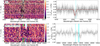 |
Fig. 1 Residuals maps and transmission spectra around the Hα line (top panels) and He I NIR triplet (bottom panels) lines for TOI-1136 d observations. Hα results are the combination of HARPS-N and CARMENES VIS observations. He I triplet results are from CARMENES NIR observations. Left panels: residual maps in the stellar rest frame. Time since mid-transit time (Tc) is shown on the vertical axis, wavelength is on the horizontal axis, and relative absorption is colour-coded. The dashed and dotted white horizontal lines indicate the different contacts during the transit. The dashed cyan tilted lines indicate the predicted trace of the planetary signals. The solid green vertical lines indicate the position of the OH emission telluric lines. The solid blue line indicates the position of the H2O absorption telluric line. Right panels: planet transmission spectra (TS) in the planet rest frame. We show the original data in light grey and the data binned by 0.2 Å in black. When an absorption signal is fitted, a red line and shaded region show the best Gaussian fit model with its 1σ uncertainties. The dotted cyan vertical lines indicate the Hα (top) and the He I triplet (bottom) lines positions. All the wavelengths in this figure are referenced in a vacuum. |
3 Transmission spectroscopy results
In this section we present the results and the details of the residuals maps and TS calculations planet by planet. We present an example of a residuals map and TS figure in Figure 1. Here, we describe the planets in which a detection signal is found, while the rest of the planets are presented in Appendix B. The figures for the rest of transits without detections are shown in Appendix A of the supplementary material. Furthermore, the time evolution of the activity indicators derived from the analysed transits can be found in the SM Appendix A as well.
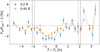 |
Fig. 2 Transit light curve of Hα line from the combined observations of TOI-1136 d. The Hα light curve was constructed integrating the counts of the residual map in the planet rest frame around λ0 using σ (blue) and FWHM (orange) wavelength band passes from Table H.1. The vertical lines represent the different contacts during the transit. |
3.1 TOI-1136 d
One HARPS-N transit of TOI-1136 d was observed to check for the planetary RM signature in the RV time series (Dai et al. 2023a). In this work, we inspected the dataset looking for Hα planetary absorption signal. Furthermore, we scheduled a second transit with CARMENES to inspect the whole spectral range. We used nonlinear ephemerides to determine the Tc for the second transit (F. Dai, priv. comm.). The RM and CLV effects over the final TS of Hα and He I triplet lines are negligible (Fig. H.1). Thus, we did not correct the data from these marginal effects.
The residual maps and TS of the Hα for the individual nights are shown in Fig. A.14, while the final results are shown in Figure 1. HARPS-N results show a noisy TS with a small absorption feature. However, a similar feature is also detected in the CARMENES Hα TS, which has higher S/N. The results from both nights confirm the Hα detection on the atmosphere of TOI-1136 d. The combined Hα residual map and TS are shown in Fig. 1. We fitted the signal obtaining an absorption of  . Table H.1 presents the priors and posteriors, and Fig. H.2 shows the posterior distributions. Although the signal is a bit deeper in the first half of the transit, the Hα transit light curve (Fig. 2) shows an absorption consistent with the transit duration without evidences of tail-like structure.
For the He I triplet, because the CARMENES observations were performed close to the end of the night, the last spectra are affected by solar He I emission. Although we corrected the emission line, some residuals still persisted. Then, we decided to mask the affected spectral range only on particular spectra. The He I residual map and TS are shown in Fig. 1, and do not show clear evidences of He I absorption. We placed a 3σ upper limit to the He I triplet excess absorption of ~0.5%.
3.2 TOI-1268 b
The transit of TOI-1268 b on the 24 of February 2023 was only followed spectroscopically by GIANO-B, and we missed the information about Hα, and the stellar variability or activity from the visible wavelength range covered by HARPS-N. MuSCAT2 covered the same transit photometrically with the exposure times initially set to 𝑔 = 5 s, r=10 s, i=10 s, and ɀs=15 s and later modified to 𝑔=5 s, r=10s, i=8 s, and ɀs=12 s to avoid the saturation of the target star. Our MuSCAT2 transit fit ha a central time of Tc = 2460000.66841 ± 0.00014 BJD.
The four bands of the MuSCAT2 photometry do not show the presence of strong stellar activity or the planet crossing in front of any big starspot(s). Moreover, the Pa-β, Pa-γ, and Pa-δ lines are mainly flat with no correlation with the stellar He I line. Because our observations ended close to the twilight, our last spectra are affected by He I sunlight contamination. Because this kind of emission increases quickly between exposures as the observations are approaching the twilight, it is not well corrected by the ABAB procedure. We decided to mask those regions affected by the He I emission only in the selected spectra.
The residual map and TS are shown in Fig. 3, where the residual map shows an absorption region at the expected position of the planetary trace. The signal is well detected in the residual map and the TS, where we fitted a blue-shifted absorption of  (EW= 19.1±1.9mÅ). Table I.1 presents the priors and posteriors, and Fig. I.2 shows the posterior distributions. These high-resolution spectroscopy results confirm the He I detection using narrow-band photometry from Pérez-González et al. (2024). We also constructed the He I triplet transit light curve, shown in Fig. 4. The absorption seems to extend further than the end of the white light transit hinting an He tail, that needs to be confirmed in further observations.
3.3 TOI-2018 b
The planet candidate TOI-2018 b was initially alerted to the community as a ‘young planet’, but final analyses of its age were ambiguous and it was not possible to confirm an age below 1 Gyr ( ; Dai et al. 2023b). Although we can not include TOI-2018 b in our sample of young planets, the results obtained from two partial transits observed with GIARPS deserve to be included in this work.
The GIARPS transit on the night of 15 June 2023 was photometrically followed with MuSCAT2, observing the transit in four bands with the exposure times set to 𝑔=15 s, r=15 s, i=10 s, and ɀs=10 s. Our MuSCAT2 transit fit found a central time of Tc = 2 459 746.4287±0.0021 BJD, confirming that we missed partially the transits in both visits.
The Hα residual map and TS from the individual nights and their combination are shown in Figs. A.19 and 5, respectively. The TS is flat, and the 3σ upper limit for Hα excess absorption is set to 1.5%.
The He I triplet residual map and TS from the individual nights and their combination are shown in Figs.A.20 and 5, respectively. Although the quality of the two nights is different, the results of both nights are consistent within 2σ, and we detect a consistent excess absorption of ~1% at the expected position of the planetary He I signal. When we combine both nights, we confirm the detection of a red-shifted He I absorption of  (EW = 7.8± 1.5 mÅ). All the nested sampling material for the individual and combined datasets is shown in Appendix L. The He I triplet transit light curve (Figure 6) shows an absorption signal consistent with the transit duration, with no evidence of an extended He signal. Although the He I signal is consistent and well detected in the two parcial transits, a full transit observation will help to confirm our detection and the study of TOI-2018 b atmospheric evaporation.
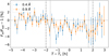 |
Fig. 4 Transit light curve of He I triplet from TOI-1268 b detection. The He I light curve was constructed integrating the counts of the residual map in the planet rest frame around λ0 using σ (blue) and FWHM (orange) wavelength band passes from Table I.1. The vertical lines represent the different contacts during the transit. |
4 Additional literature evaporation tracers observations
4.1 Young planets from the literature
In the framework of the MOPYS project, we adopted the 1 Gyr stellar age as the threshold to classify exoplanets as young (≲ 1 Gyr) or old (≳ 1 Gyr). We used this nomenclature in the discussion in Section 6. The 1 Gyr threshold is mainly based on the core-powered evaporation timescale, which is longer than the strong photo-evaporation initial stage (X-ray driven).
Young exoplanets are an interesting population that have called the attention of different research groups. To put the young planet results obtained in this work into context, we inspected the ExoAtmospheres6 database looking for other young exoat-mospheric analyses. Table 2 presents a compilation of literature high-resolution spectroscopy studies of young transiting exo-planet atmospheres targeting the Hα or the He I triplet7. Here, we give a short context to those observations from the literature included in Table 2.
KELT-9 b: As the hottest exoplanet known to date, this planet attracted attention to probe and investigate its extreme atmosphere. Yan & Henning (2018) detected an evaporating exosphere of Hα. However, Nortmann et al. (2018, see supplementary material section therein) could only place an upper limit to the He I triplet absorption.
K2-25 b: The He I triplet was observed using the IRD spec-trograph, although the transit was contaminated by telluric OH emission. Gaidos et al. (2020b) reported a 99% confidence upper limit to the transit-associated EW of 17 mÅ.
AU Mic b: Due to the host star’s youth, the Hα observations with ESPRESSO were strongly affected by stellar activity, making it impossible to set an upper limit (Palle et al. 2020b). Recently, Rockcliffe et al. (2023) reported a Lyα detection but only in one of the two visits with HST/STIS. IRD and Keck/NIRSPEC spectrographs obtained a 99% confidence upper limit to the He I EW of 4.4 and 3.7 mÅ, respectively (Hirano et al. 2020). Allart et al. (2023) observed one transit with SPIRou spectrograph finding a significant He I absorption feature (0.37 ± 0.09%). However, the authors finally reported a conservative 3σ upper limit of 0.26%, consistent with previous observations.
K2-136 c: Gaidos et al. (2021) put a 99% confidence upper limit to the He I triplet EW of 25 mÅ with one transit observed with the IRD spectrograph. The He I lines position in between the telluric OH emission and H2O absorption lines complicated the calculation of the transmission spectra.
DS Tuc b: The Hα was analysed with ESPRESSO and HARPS spectrographs observations. However, the transits were affected by stellar activity and an Hα upper limit could not be set (Benatti et al. 2021).
V1298 Tau system: This 20-Myr old multi-planet system has seen different attempts to study the presence of He I in their planetary atmospheres. Gaidos et al. (2022) used the IRD spec-trograph to observe, during different nights, the star alone and a transit of planet b. An increasing He I absorption was detected during the transit, but the authors proposed other explanations besides the planetary absorption. Using the narrowband helium filter technique, Vissapragada et al. (2021) observed the transits of planets b and d. For planet b they do not require extra absorption to explain the flux decrease, while they found a tentative excess absorption combining two partial transits of planet d, but it requires a significant transit time variation.
WASP-52b: The planet was observed with ESPRESSO detecting Hα, and other atomic species as well (Chen et al. 2020). The presence of He I in its atmosphere has been studied, first with a tentative detection using narrow-band photometry (Vissapragada et al. 2020, 2022a) and later confirmed with the Keck/NIRSPEC spectrograph (Kirk et al. 2022). However, a recent paper by Allart et al. (2023) did not find He I absorption in two visits with the SPIRou spectrograph, and derived a 3σ upper limit of 1.69%.
HAT-P-70 b: The atmosphere of this ultra-hot Jupiter was inspected by Bello-Arufe et al. (2022) using HARPS-N. They detected absorption coming from the Hα, Hβ, and Hγ lines, and many other atomic and molecular species as well.
WASP-80 b: Its atmosphere has been targeted in search of He I absorption but without success (Fossati et al. 2022; Allart et al. 2023). Salz et al. (2015) is the only reference which provides a formerly calculated age of <200 Myr. However, the observed X-ray luminosity (log LX ~27.8 erg s−1 in Salz et al. 2015, down to 27.5 erg s−1 in Sanz-Forcada et al., in prep.) yields a log LX/Lbol~−5.0, implying an age of ~3 Gyr using Sanz-Forcada et al. (2011) age–LX relations. Moreover, the TESS light curve do not suggest a rotational period of ≲15 d. Therefore, WASP-80 is probably older than 1 Gyr according to the gyrochronology method shown in Fig. K.3 (G − J = 2.05).
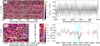 |
Fig. 5 Same as Fig. 1, but for TOI-2018 b combined observations of Hα with HARPS-N and He I triplet with GIANO-B. |
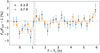 |
Fig. 6 Transit light curve of He I triplet from the combined nights of TOI-2018 b. The He I light curve was constructed integrating the counts of the residual map in the planet rest frame around λ0 using σ (blue) and FWHM (orange) wavelength band passes from Table L.3. The vertical lines represent the different contacts during the observation. |
4.2 Older planets from the literature
To put in context the young exoplanet He I (planets with ages ≲1 Gyr) findings, we complemented them with old exoplanet high-resolution He I observations (planets with age ≳1 Gyr) from the literature. We have compiled a He I triplet database, detailed in Table M.1 in the supplementary material, which we constructed using the ExoAtmospheres database and literature results. For consistency, we only considered He I triplet results from high-resolution spectrographs. That is, the narrowband photometry detections of HAT-P-26 b (Vissapragada et al. 2022b) and TOI-1420 b (Vissapragada et al. 2024) were not included8. Although we analysed the Hα and we cited some results on the Lyα as well, Table M.1 only reports the H (Hα or Lyα) observations for the planets with He I triplet observations, except for the young hot Jupiter HAT-P-70 b with Hα detection (Bello-Arufe et al. 2022). The young Neptune DS Tuc b is not included in Table M.1 because no upper limit could be set from Hα observations (Benatti et al. 2021) and no He I triplet observations could be found in the literature.
Given the number of planets and details of each observation, we do not discuss the planets individually here. We refer to Table M.1 and the appropriate references.
4.3 A note on He I variability
The planetary He I triplet is known to show variability in its strength but also in its detectability (e.g. Palle et al. 2020a; Zhang et al. 2022a). In this work, we presented two upper limits for TOI-2O76b and TO 1683 b, for which Zhang et al. (2023b) reported He I detections. Our upper limits are consistent at 1σ with Zhang et al. (2023b) detections. Thus, He I triplet variability may be one reason for our absence of planetary signals. Variability was also invoked by Orell-Miquel et al. (2023) to explain the ~2σ deeper absorption found in HD 235088 b. We note that Gaidos et al. (2023) derived non-conclusive results for TOI-2076 b He I signal, and TOI-1683 b transit from Zhang et al. (2023b) was performed in poor observing conditions. We want to stress the importance of re-observing targets as a sanity check to confirm previous results (detections or upper limits), but also to study the planetary He I triplet variability.
On the other hand, Krolikowski et al. (2024) analysed the variability of the He I triplet of young stars. In particular, Vl298 Tau, K2-100, K2-136, K2-77, HD 63433, and TOI-2048 were in the list of observed stars. They found that young stars show higher variability, with Vl298 Tau being extremely variable, which could explain the non-conclusive results from the He I observations. The stellar He I variability decreases rapidly and keeps constant for stars older than ~300 Myr (Krolikowski et al. 2024). Although the stellar Hei triplet line is variable, the short-term variability might not have a significant impact on the transit observations performed during the same night (Fuhrmeister et al. 2020; Krolikowski et al. 2024). In fact, Hα is more sensitive to stellar variability than the He I triplet (Fuhrmeister et al. 2020) and the analyses of those lines on AU Mic b and DS Tuc b are good examples (Palle et al. 2020b; Hirano et al. 2020; Benatti et al. 2021).
5 Criteria for detections, non-detections, and non-conclusive measurements
A problem we encountered when studying the He I signal (and Hα as well) was how to deal with the observations where only an upper limit value is given, which are the majority of the cases (52 of 69 in Table M.1). In this work, we classified the upper limit measurements in two groups: a) non-conclusive measurements (i.e. the upper limit value is large, and it does not actually constrain the presence of the atom in the exoplanet atmosphere) and b) non-detection (i.e. the upper limit value is low enough to confidently assume there is no significant presence of that atom in the exoplanet atmosphere).
To assign observations to either category, for the He observations, we used the relationship that the observed and theoretical mass-loss rates (ṁobs and ṁtheory, respectively) seem to follow, represented in Figure 7. We present ṁobs and ṁtheory equations in Sect. 6.3, and we further explore and discuss the trend in that section. For the time being, the fitted line between ṁobs–ṁtheory seems to account for the differences between planetary characteristics, and populations (Vissapragada et al. 2022b; Zhang et al. 2023a, and Sect. 6.3). Therefore, we consider that relation to classify the He I upper limits. Although other criteria might be chosen, it is used consistently for the whole sample.
We computed the ṁobs upper limits from the He I EW upper limit values. If the ṁtheory upper limit falls above the fitted line, the ṁobs upper limit value is higher than the a priori expected signal, and so it is not constrained. Thus, we refer to those measurements as non-conclusive (orange down-pointing triangles in Fig. 7). On the other side, the ṁobs upper limits falling below the line can be considered as non-detections (red crosses in Fig. 7). We also considered as non-detections the ṁobs upper limits that fall within 1σ of the fit (grey shaded are in Fig. 7).
We note that Fxuv is unknown for some of the exoplanets in our sample. For those planets with no measured FXUV, we performed a similar procedure but in a 1/ρXUV versus mobs diagram (not shown), which is a proxy for ṁtheory versus ṁobs · ρXUV is the planet density when considering as the radius its XUV radius, which is different from the planet density ρp (see Sect. 6.3).
We did some exceptions when classifying some He I observations. GJ 1214 b: we re-classified as a non-detection the tentative He I signal reported by Orell-Miquel et al. (2022) due to other upper limits reported in the literature (Petit dit de la Roche et al. 2020; Kasper et al. 2020; Spake et al. 2022; Allart et al. 2023). V1298 Tau b: because of the unclear origin of the signal detected by Gaidos et al. (2022), we set this observation as non-conclusive. V1 298 Tau c is in the same situation as planet b, and its He I upper limit is non-conclusive. Moreover, the measurements for the V1298 Tau planets are consistent with the stellar He I line variability range derived for their host star (Krolikowski et al. 2024). WASP-76b: its He I feature was presented as upper limit in Casasayas-Barris et al. (2021a) but here we consider it as a non-detection due to the planet position well below the ṁobs–ṁtheory line.
For Hα, we simply considered the upper limits as non-detections. However, if the Hα upper limit absorption is comparable to that of He I, we used the He I classification for both measurements. We only considered few Lyα detections for some particular exoplanets. The classification and nomenclature described in this section (detection, non-detection, and non-conclusive) is used all across the manuscript.
We note that absoprtion measurements of the three lines (Lyα, Hα, and He I triplet) would be the ideal case to determine whether an exoplanet is undergoing strong atmospheric escape. However, these observations are not available for all targets, and may be hard (even impossible) to obtain for some individual stars (e.g. Lyα interstellar medium extinction, Hα variability in active stars, or low He I triplet population). When possible, we consider the results from the three lines to determine atmospheric escape detections.
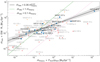 |
Fig. 7 Relationship between the observed (ṁobs) and the theoretical (ṁtheory) energy-limited mass-loss rates. We define XUV until the He I ionisa-tion range (λ = 5–504 Å). The black line indicates the fitted relationship (shown in the legend) and the shaded area the 1σ uncertainty. He I observations are coded as blue circles for detections, red crosses for non-detections, orange down-pointing triangles for non-conclusive. We did not plot the error bars of ṁtheory due to the very large uncertainties associated with the FXUV values and its calculation. Every planet has its name labelled: in black for detections and the others in grey. The two new detections presented in this work, TOI-2018 b and TOI-1268 b, are in good agreement with the predicted trend. |
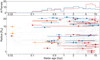 |
Fig. 8 Planetary radius vs stellar age diagram of evaporation (H and He I) detections (blue circles), non-detections (red crosses), and non-conclusive observations (orange down-pointing triangles). Planetary radii and stellar ages are from Table M.1. The top panel shows the summed histogram of evaporation detections (blue line) and non-detections (red line) across stellar age. The grey points represent all known planets with radius and age determined with precision better than 30% and 50%, respectively (data from NASA Exoplanet Archive). |
6 Discussion
We have organised the discussion of our results in the following manner: Section 6.1 gives a general view of the evaporation tracers across stellar age, planet radius, period, and mass. In Sect. 6.2 we constrain the cosmic shoreline from He I detections. In Section 6.3 we explore the relation between He I detections and the energy-limited mass-loss rates. Finally, we explore further relations between He I detections and different planet and stellar properties in Sections 6.4, 6.5, and 6.6.
6.1 Evaporation tracers of planetary atmospheres across stellar age
Figure 8 displays the planetary radius versus stellar age, with the planets colour-coded according to their evaporation measurements. We considered the He I triplet and/or Hα absorption detections (and Lyα in some particular cases) as proxies of evaporation signs. Thus, an evaporation detection means that either He I or Hα or both have been positively detected.
Figure 9 is similar to Figure 8 but focuses only on the He I triplet, and presents a comparison between the He I EW signals and the stellar age. The planets are marked and colour-coded according to their He I results. Allart et al. (2023) reported that a trend between He I and stellar age was noticeable in their sample of eleven planets, however the authors refrained from further conclusions due to their small sample size and the lack of precise stellar ages. Although in this work we used a larger sample (18 young and 35 old planets, including detections and non-detections, but less homogeneous than the Allart et al. 2023 one), we do not notice a clear correlation between He I EW and stellar age.
The first 100 Myr are critical for the planetary atmospheric evolution, according to photo-evaporation models (see Introduction in Sect. 1). Unfortunately, there are only a few planets in Figures 8 and 9 with ages ≲ 100 Myr. The youngest objects have ages of ~20 Myr (AUMicb and V1298 Tauc & b) and then there is a lack of He I and Hα observations until ~ 100 Myr (WASP-80 b, and K2-77 b). WASP-80 b, with a formerly calculated age of <200 Myr (Salz et al. 2015), has no detection of He I triplet. However, a possible older age of WASP-80 (see Section 4.1) and the calculated log LXUV at the planet separation (Table M.1) could explain the lack of detection of the He I triplet. AU Mic b non-detection is harder to reconcile, but different scenarios can be invoked (e.g. stellar activity masking possible detections or H/He ratio). He I and Hα observations of V1298 Tau b & c resulted in non-conclusive measurements, mainly due to the strong stellar activity levels of the young host star. However, the masses derived for planets b and e indicate that their densities are similar to older planets, suggesting they are not inflated and that they contracted faster than expected (Suárez Mascareño et al. 2021).
While the non-detections of WASP-80b, AUMicb, V1298 Tau b & c do not seem to fit the predictions from photo-evaporation models (Lopez et al. 2012; Owen & Jackson 2012; Owen & Wu 2013, 2017; Owen & Lai 2018; Dawson & Johnson 2018), the sample of ≲ 100 Myr-old planets is too small to draw conclusions. A larger sample of ≲150-Myr-old planets is needed to explore the photo-evaporation timescales.
From Figures 8 and 9, the youngest planet with He I detection is TOI-1268 b (245± 135 Myr), and the youngest planet with Hα detection is MASCARA-2b ( Myr). The number of planets with evaporation detections increases until peaking at ~2 Gyr, and then it is roughly constant, but this is related to the age distribution in our sample. The proportion between detections and non-detections remains constant (within error bars) with age, except at old ages (>5 Gyr) when non-detections dominate (see Figs. 8, and 9). This non-detections domination is more pronounced when considering only the He I observations (Fig. 9), and extended over all stellar ages, except over the 1–3 Gyr range.
Our results on evaporation timescales agree with the conclusions from Loyd et al. (2020) on the radius gap, and Christiansen et al. (2023) on the hot Neptune population (see Fig. 6 in their work), and photo-evaporation mechanism is not more supported than the core-powered one. The fact that we do not see a decrease in the evaporation tracers, until very old ages (~5 Gyr, see Figs. 8, and 9), might be marginally more consistent with the core-powered timescale of Gyr (Ginzburg et al. 2016, 2018; Gupta & Schlichting 2020).
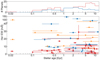 |
Fig. 9 Equivalent width (EW) of He I detections (blue circles), non-detections (red crosses), and non-conclusive observations (orange down-pointing triangles) as functions of stellar age. The top panel shows the summed histogram of He I detections (blue line) and non-detections (red line) across stellar age bins. |
6.1.1 Radius-period diagram across stellar age
Figure 10 compares the population of young (≤ 1 Gyr, top panels) and old (> 1 Gyr, bottom panels) planets in a radius-period diagrams for only He I triplet observations, only H (mainly Hα with few Lyα) observations, and both evaporation proxies. Figures 8, 9, and 10 show no clear differences for the evaporation of the gas giant planets before and after 1 Gyr. The detections of evaporation are evenly spread over the stellar ages, with more preference of Hα detection than from He I for the young gas giants. We note that there are no evaporation detections of young and old planets below the radius gap or for Earth-like planets, supporting rocky planets are not under extreme atmospheric mass-loss processes, at least after ~300 Myr which is the age of the youngest rocky planet in our dataset (TOI-1807 b).
Allan et al. (2024) simulated how the He I triplet planetary signal from a highly irradiated (ap = 0.045 AU) gas giant planet (Mp = 0.3 MJ) around a K-dwarf star changes with the stellar age. They assumed a typical H/He ratio of 98/2 (Lampón et al. 2020, 2021b; Orell-Miquel et al. 2023). From their simulations, they derive excess absorption peaks of 4–7% for young (16–550 Myr) Hot Jupiters, while at 5 Gyr the excess absorption would be of ~1.5%. They state that a close-in (ap < 0.1 AU) planet with a radius of 1–2 RJ transiting a <150-Myr-old K dwarf star would be the best target to test their evolution models. Although the He I triplet detection is favoured by the extreme radiation in XUV range (λ < 504 nm; Sanz-Forcada & Dupree 2008) and the TS simulations from Allan et al. (2024), none of the three 20-Myr-old planets analysed here present a clear detection of He I. WASP-80b (ap =0.035 AU, Rp = 1 RJ, Mp = 0.5MJ, <200Myr, spectral type ~K7V) is the closest planet from Table M.1 to the simulated one in Allan et al. (2024) but it has very low He I upper limits (Fossati et al. 2022; Allart et al. 2023). WASP-52 b might be in agreement with the simulations, although the largest He I excess absorptions to date come from older planets (e.g. HAT-P-67 b, Gully-Santiago et al. 2024; HAT-P-32 b, Czesla et al. 2022; and WASP-107 b, Kirk et al. 2020). In Fig. 10 WASP-52 b is the only young gas giant planet with a He I detection. The ratio of He I detections to non-detections seems larger for old rather than young planets, but there are fewer differences when comparing the H detections to non-detections.
6.1.2 Small planet evaporation across stellar age
Figure 11 shows the radius-mass diagram for small planets (Rp <5 R⊕ and Mp < 30 M⊕), also comparing evaporation proxies for young and old planets. Planets with Rp ~ 1.5–3 R⊕ fall in a degenerated region of the mass-radius diagram, and their bulk compositions can be consistent with a large range of models, from water worlds (planets with a large water mass fraction) to planets with rocky cores with H/He envelopes (Zeng et al. 2019). For these planets, in Fig. 11, we found a mixture of detections and non-detections, with no difference between young and old planets.
Planets with Rp > 3 R⊕ are well above the water-rich composition line and are supposed to be gaseous with very light envelopes and low densities (Luque & Pallé 2022). In our sample there are four young and five old puffy planets with evaporation observations (see right panels of Fig. 11). While only 1 in 4 young planets has an evaporation detection, 3 out of 5 old planets have a detection, hinting that atmospheric escape of puffy sub-Neptunes is stronger at ages older than ~1 Gyr. Still, the numbers are small, and a larger sample is needed to confirm these findings.
For the planets above the radius valley, Malsky et al. (2023) predicted a He enhancement due to the diffusive separation of the atmospheric constituents where the He and metals are preferentially retained while H is evaporated. The timescale of this mechanism is comparable to the planet lifetime (~ 10 Gyr) and planets with ≲ 1 Gyr have not had time to show the effects of favoured H evaporation (Malsky et al. 2023). So, our young planet population is too young to suffer this differential escape process, and even some of our old planets could be considered young as well. Then, the long timescale might explain why Figure 11 does not show more He I detections for the old waterworlds than for the young ones. Malsky et al. (2023) predict that TOI-1235 b will have an He enhanced atmosphere at 10 Gyr, but Krishnamurthy et al. (2023) put a very restricted He I upper limit, although its age is poorly constrained  . The other planets listed in Malsky et al. (2023, Table 1) have no H/He observations to test their predictions.
Although Malsky et al. (2023) focus only on the small planet population (≲ 3 R⊕), the diffusive separation and the subsequent preferential H evaporation could be the mechanism to explain some observational results from Figs. 10 and 11 regarding large and intermediate-sized planets, (i) There are no He I detections in young puffy planets but there are for old ones. TOI-1136 d is the only young puffy planet with Hα detection, and the only three old puffy planets with H observations both show H evaporation, (ii) WASP-52 b is the only young gas giant with He I detection (and also has Hα detection) while there are several detections on old gas giants, and Hα is extensively detected in young and old gas giant planets.
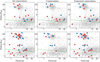 |
Fig. 10 Radius-period diagrams for planets with ages ≤ 1 Gyr (top panels) and >l Gyr (bottom panels) with He I (left panels) and H (Hα or Lyα. middle panels) observations, and evaporation (combination of He I and/or H observations, right panels). Detections and non-detections are marked as blue circles and red crosses, respectively. The radius gap (Van Eylen et al. 2018) is marked as a dashed green line. The grey points represent all known planets with period and radius determined with a precision better than 25% (data from NASA Exoplanet Archive). |
6.2 Cosmic shoreline from He i observations
The cosmic shoreline (Zahnle 1998) is an empirical division found in the Solar System bodies that splits them between those that retain a certain amount of atmosphere and those that are purely bare rocks without atmosphere. The division was extended to the extrasolar planet population with success by Zahnle & Catling (2017). Determining precisely the cosmic shoreline is important as it has often been used to predict the existence of an atmosphere for newly discovered planets, and to argue for atmospheric characterisation follow-up (e.g. with the James Webb Space Telescope). Observationally, extended atmospheres are relatively easy to detect via H and He I absorptions. Here, we use these observations to better constrain the cosmic shoreline.
Zahnle & Catling (2017) found a power law between planet bolometric instellation (Ip) and planet velocity escape υesc that follows Ip ∝ υesc4. However, the radiation that shapes the exoplanet atmosphere is the X-rays and EUV stellar flux received by the planet during its early stages. Zahnle & Catling (2017) assumed the approximation of X-ray luminosity saturation (Jackson et al. 2012) to estimate the total extreme radiation (X+EUV radiation) received by the planet. Following Zahnle & Catling (2017, Eq. (27)), we compute the cumulative X-rays and EUV instellation (IX+EUV ; considering λ < 100 nm) as a function of the planet instellation (Ip) and the stellar bolometric luminosity (L★):
 (2)
(2)
We computed υesc as
 (3)
(3)
where G is the universal gravitational constant. The empirical relation found between IX+EUV with υesc also follows the same power law (IX+Euv ∝ υesc4), as for Ip.
Zahnle & Catling (2017) presented the relationships between Ip and υesc, and between IX+EUV and υesc for the planets and small bodies of the Solar System along with the exoplanet population. To test the predictions of the cosmic shoreline, we compared the proposed empirical relationships to the actual He I detections. Figure 12 reproduces Figs. 1 and 2 from Zahnle & Catling (2017), and includes also the He I observations. Because the cosmic shorelines are empirical relations, only the slope in logarithmic scale is determined. Thus, we get from Zahnle & Catling (2017, Figs. 1 and 2) the independent terms to plot the empirical equations.
By definition, all He I (and Hα) detections must be below the cosmic shorelines plotted in Fig. 12. However, we find seven gas planets with He I (or Hα) detections in the region of supposedly bare rocky planets. Those are the ones labelled in Fig. 12 panels. In Fig. 12 left panel, HAT-P-32b and HAT-P-67 b are clearly located above the line, although their 1 σ uncertainties fall in the limit of the cosmic shoreline. TOI-1136 d, WASP-76 b, and KELT-9 b which have He I non-detections but Hα detections, are also over or above the cosmic shoreline. Moreover, in Fig. 12 right panel, HAT-P-32 b and WASP-107 b fall over the line, and GJ 3470 b and TOI-1136 d are clearly above the cosmic shoreline for energy-limited regime. With the exception of TOI-1136 d, the planets that contradict the shoreline are not young planets, with stellar ages > 1 Gyr.
Zahnle & Catling (2017) stated that the I ∝ υesc4 and IX+EUV ∝ υesc4 lines are ‘drawn in by hand to guide the eye’. Thus, the evaporation detections above the shoreline can help to constrain the independent terms of those by-hand equations. For that purpose, we considered the planet whose uncertainties have the largest separation from the by-hand line to compute the limits of the cosmic shoreline. We took the coordinates of the extreme uncertainty as a point to calculate the line equation. We took HAT-P-67 b for the I ∝ υesc4 line, and GJ 3470 b for IX+EUV ∝ υesc4 although very similar results were obtained with TOI-1136 d. Then, it is trivial to get the line equation with the slope and one point. The cosmic shoreline equations constrained from the evaporation detections are
![Mathematical equation: $\log \left( {I/{I_ \oplus }} \right) = 4\log \left( {{\v _{{\rm{esc}}}}\left[ {{\rm{km}}\,\,{{\rm{s}}^{ - 1}}} \right]} \right) - 2.04$](/articles/aa/full_html/2024/09/aa49411-24/aa49411-24-eq35.png) (4)
(4)
and
![Mathematical equation: $\log \left( {{I_{{\rm{X}} + {\rm{EUV}}}}/{I_{{\rm{X}} + {\rm{EUV}} \oplus }}} \right) = 4\log \left( {{\v _{{\rm{esc}}}}\left[ {{\rm{km}}\,{{\rm{s}}^{ - 1}}} \right]} \right) - 2.51.$](/articles/aa/full_html/2024/09/aa49411-24/aa49411-24-eq36.png) (5)
(5)
They are shown in Figure 12 left and right panels as dashed black lines, respectively. In both cases, the cosmic shoreline moved to higher radiation levels reducing the amount of exoplanets with no atmosphere. Further atmospheric observations and more precise measurements of the planets close to the shoreline will allow a better constraint of the observed cosmic shoreline.
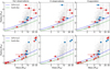 |
Fig. 11 Radius-mass diagrams for planets with ages <1 Gyr (top panels) and >1 Gyr (bottom panels) with He I (left panels) and H (Hα or Lyα, middle panels) observations, and evaporation (combination of He I and/or H observations, right panels). Detections and non-detections are marked as blue circles and red crosses, respectively. The solid lines are the theoretical models from Zeng et al. (2019) for Earth-like (green) and 50% H2O+50% rocky (blue) compositions. The grey points represent all known planets with mass and radius determined with a precision better than 20% (data from NASA Exoplanet Archive). |
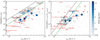 |
Fig. 12 Cosmic shoreline compared to He I observations. He I non-detections are denoted by red error bars with no marker. He I detections are circles scaled by their Rp and colour-coded by their stellar age (lateral colour bar). Instellation relative to Earth vs escape velocity (left panel) and cumulative instellation in the XUV range relative to Earth vs escape velocity (right panel) graphics. We marked the cosmic shoreline, as I ∝ υesc4, from Zahnle & Catling (2017, solid green line) and constrained from the observations (dashed black line). Planets sitting above or on the cosmic shore and with H/He detections are labelled. |
 |
Fig. 13 He I transmission signal strength for the planets with detections (blue circles with error bars in black) and non-detections (red down-pointing triangles in grey) as a function of the stellar FXUV (λ = 5– 504 Å) at the planet distance. We show the equivalent height of the He I atmosphere, |

6.3 Observed versus theoretical mass-loss rates
Since the first He I detection in planetary atmospheres, there have been many attempts to predict the presence of this line using other observable planetary parameters. Nortmann et al. (2018) performed one of the first attempts by computing  . That is: the equivalent height of the He I absorbing atmosphere
  , where DHe is the He I absorption peak in %, divided by the atmospheric scale height Heq = (kB Teq)/(µ𝑔p), where kB, µ, and 𝑔p are the Boltzmann constant, the mean molecular mass, and planet gravity, respectively. Figure 4 in Nortmann et al. (2018) presented a correlation between the He I absorption signal and FXUV (λ = 5 − 504 Å), but with a sample of only five planets. Figure 13 reproduces the same diagram with the current set of 43 He I observations (detections and non-detections with FXUV measurements). The trend is not that clear and there is no evident pattern between detections and non-detections, maybe due to the non-uniformity of the sample (e.g. different instruments and data analysis techniques).
Rather than using the strength of the He I absorption, Vissapragada et al. (2022b), and later Zhang et al. (2023a), explored the relation between the mass-loss rates derived from the observations (ṁobs) as a function of FXUV/ρp (ρp is the planet density). While Vissapragada et al. (2022b) derived the observed mass-loss rates comparing the measured excess transit absorptions with a grid of Parker wind models, Zhang et al. (2023a) estimated the observed mass-loss rates from an order-of-magnitude method. Furthermore, Zhang et al. (2023a) found that the theoretical maximum energy-limited mass-loss rate (ṁtheory) is proportional to FXUV/ρXUV (ρXUV is defined below). However, they reported very similar results when using FXUV/ρp. Despite those differences, both works found a positive correlation between ṁobs and FXUV/ρp, and, their energy-limited outflow efficiencies agree within uncertainties (Vissapragada et al. (2022b):  ; Zhang et al. (2023a): η0 = 0.31 ± 0.06).
Here, we focus on the relationship between ṁobs and ṁtheory, while adding the two new He I detections presented in this work (TOI-1268 b and TOI-2018 b), which is the main difference with the study performed by Zhang et al. (2023a). For consistency, we followed the indications from Zhang et al. (2023b,a) to compute the ṁobs–ṁtheory diagram with our set of He I observations.
We made the same assumptions as in Zhang et al. (2023b,a) to calculate ṁobs with the order-of-magnitude method as
 (6)
(6)
Equation (6) is computed in cgs units, where me is the electron mass, mHe is the He atomic mass, cs is the sound speed (assumed to be cs = 10 km s−1), c is the speed of light, EW is the equivalent width of the He I signal, R★ is the stellar radius, 0.25 comes from assuming that 25% of mass out-flow is He (atoms or ions), f is the fraction of He atoms in the metastable ground state (assumed to be f = 10−6), e is the electron charge, λ0 is the He I wavelength (fixed to 10 833.3 Å),  is the sum of the product of the degeneracy and oscillator strength over the three lines of the He I triplet which is 1.62 (Zhang et al. 2023a).
The theoretical maximum energy-limited mass-loss rate (ṁtheory; Caldiroli et al. 2022; Zhang et al. 2023a), assuming that all the XUV flux received by the planet is spent on evaporation, is computed as
 (7)
(7)
where FXUV is the XUV flux (λ = 5 − 504 Å), Rxuv is the planetary XUV photosphere radius, G is the gravitational constant, Mp is the planet mass, and ρXUV is the planet density using the RXUV. We followed the equations and indications from Wang & Dai (2018); Zhang et al. (2023b,a) to estimate RXUV as
 (8)
(8)
where
 (9)
(9)
In Eqs. (8) and (9), P is the pressure at the white-light planet radius (assumed P = 100 mbar), µ is the (dimensional) mean molecular mass (we assumed µ =1.3 × mH; mH is the H atomic mass), kB is Boltzmann constant, Teq is the equilibrium temperature, Mc is the planet mass core, and ρatm.XUV is the planet atmosphere’s density at the RXUV layer. We approximated Mc ≃ Mp and used ρatm.XUV = 10−15 g cm−3. Our computed values for ρXUV are consistent within errors with those presented in Zhang et al. (2023a, Table 3).
Figure 7 presents our computed observed and theoretical mass-loss rates, recovering the predicted positive correlation for the He I detections. For a quantitative analysis, we fitted a power law as ṁobs = η0 (ṁtheory)α. We used scipy’s orthogonal distance regression to fit the equation log10(ṁobs) = α log10(ṁtheory) + log10(η0). We obtained an energy-limited efficiency of η0 =0.35 ± 0.04, which is consistent with the previous derived values (Vissapragada et al. 2022b:  ; Zhang et al. 2023a: η0 = 0.31 ± 0.06). TOI-1268 b and TOI-2018 b positions in the diagram agree with the previous detections, and they are over the fitted line. For the linearity between log mass-loss rates, we got α =0.43 ± 0.05, also consistent with Zhang et al. (2023a, α = 0.50 ± 0.08). When using ρp instead of ρxuv, we get slightly larger uncertainties for η0 and α but consistent within uncertainties (η0 = 0.39± 0.06, α = 0.42 ± 0.06).
If the evaporation on those planets was in the energy-limited regime, they should exhibit a linear relation between ṁobs and ṁtheory. Although we computed the mass-loss rates as an order-of-magnitude and with some approximations, α is ~11σ apart from 1. We find a sub-linearity relation (α ~ 0.43 < 1) and the efficiency of the ṁobs decreases with ṁtheory, as already pointed out by both Vissapragada et al. (2021) and Zhang et al. (2023a). However, this is in agreement with the theory as models predict that as the FXUV increases, the photo-evaporation escape begins to lose efficiency via radiative cooling (e.g. Murray-Clay et al. 2009; Caldiroli et al. 2022). The H/He ratio or different hydro-dynamical regimes (e.g. Lampón et al. 2020, 2021b,a, 2023) may also contribute to derive a sub-linear relation.
Along the ṁobs–ṁtheory sub-linearity, five planets (TOI-2134 b, TOI-2018 b, HD 235088 b, HAT-P-11 b, and HAT-P-18 b) show an unphysical >100% photo-evaporation efficiency. ṁtheory, as it is computed in Eq. (7), assumes the photo-evaporation scenario. However, there are other mechanisms that could enhance the atmospheric mass-loss, namely the core-powered and the Roche lobe overflow. The core-powered mechanism may contribute in the atmospheric escape of those planets as they are relatively young (except HAT-P-11 b and HAT-P-18 b). However, a core-powered contribution can not be confidently assumed in those planets, as other parameters as the H/He ratio, the stellar flux or the atmospheric heating efficiency may contribute to change the derived ṁobs–ṁtheory relation and yield unrealistic efficiencies. On the other hand, Roche lobe overflow is not expected, as these planets are not extremely close-in. Non-thermal processes (e.g. ion pick-up or sputtering) may also help to achieving a > 100% efficiency in those planets (Güdel et al. 2014).
6.4 He I dependence with the Hill radius
Because the FXUV is a critical factor for the detectability of extended He atmospheres via the He I triplet in the NIR (Sanz-Forcada & Dupree 2008; Oklopčić & Hirata 2018), different relationships have been proposed, aimed at explaining the He I detections, that take into account the FXUV value, either directly (e.g. δRp/Heq−FXUV; see Fig. 13) or indirectly (e.g. ṁobs–ṁtheory; see Fig. 7).
Here, we explore other relationships that might explain the He I signals but accounting also for the differences between system characteristics, as  . We considered the dimen-sionless parameter RHe/RHill which is the division between the apparent radius of the planet at the He I triplet wavelength by the Hill radius of the planet. We computed the RHe as
 (10)
(10)
where DHe is the He I absorption. The equation for the RHill is
 (11)
(11)
As in Eq. (1), we did not take into account planet’s eccentricity. Compared to ṁobs, RHe/RHill takes into account the He I absorption peak instead of the EW of the signal, and the relation between masses of the system and the ap instead of the star radius. Figure 14 presents Rнe/RHill as function of the ṁtheory· As it is shown, He I detections are aligned in the diagram, hinting that the dimensionless parameter RHe /RHill is a good indicator to investigate He I correlations. RHe/RHill–ṁtheory have a Pearson correlation r = 0.9034, and we obtained a very similar correlation with ṁobs–ṁtheory (r = 0.8985). For a more quantitative analysis, we fitted the trend that seems to be between RHe/RHill and ṁtheory. Using the same code as in Sect. 6.3, we fitted the equation RHe/RHill = A log10(ṁtheory) + log10(B) and we get A = 0.213±0.027 and B = 2.58±0.15.
We find that gas giant planets are able to fill a larger fraction of their Hill radius (or Hill sphere) than mini-Neptunes. However, He I detections on mini-Neptunes have comparable RHe/RHill values to those from larger planets such as HD 189733 b or TOI-1268 b. This result could point to an observational bias for small planet observations where we are only detecting those exoplanets that their He signal is RHe/RHill ≳ 0.2. Moreover, compared to Fig. 7, some planets move from one side to the other of the line defined by the He I detections, finding planets coded as non-detections above the line or upper limits under the line. TOI-1807 b is a clear example of a non-detection above the line. In particular, the planets with low ṁtheory value seems to be consistently above the line, which could indicate another bias as well. But, this bias could be more related with the current capabilities of getting more precise measurements. Since they are likely low irradiated by FXUV from the host star, the amount of atoms of He detectable via the NIR triplet might be also very low and very challenging thus for the current telescopes and instruments. The recent He I detection on TOI-2134 b (Zhang et al. 2023a) is consistently in the lower corner on Figures 7 and 14, and might indicate the current limit in terms of signal detectability.
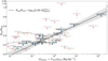 |
Fig. 14 Relationship between RHe/RHill and the theoretical (ṁtheory) energy-limited mass-loss rate. We define XUV until the He I ionisation range, λ∊5– 504 A. The black line indicates the fitted relationship (shown in the legend) and the dashed area the 1σ uncertainty. He I observations are coded as blue circles for detections, red crosses for non-detections, orange down-pointing triangles for non-conclusive. The colour-coding is according to the results from Sect. 6.3 (see Fig. 7). We did not plot the error bars of ṁtheory, due to the very large uncertainties associated with the FXUV values and its calculation. Every planet has its name labelled, in black for detections and the rest are in grey. |
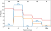 |
Fig. 15 Histogram of He I triplet observations as function of spectral types (M, K, G, F, and O, B, and A). The number of planets with detections, non-detections, and non-conclusive observations are shown as blue, red, and orange lines, respectively. We indicate the total number of inspected planets in black at the top of each column. We indicate the percentage of detections for each spectral type in blue. |
6.5 He I detections across stellar types
Oklopčić (2019) indicated that late-type stars are the most favourable host stars to detect the He I triplet on their close-in transiting exoplanets, specially the K-type stars. We explored this theoretical prediction computing the histograms of detections, non-detections and non-conclusive He I triplet observations as function of the different spectral types. Figure 15 shows that K-type exoplanet hosting stars are the most targeted ones (29 planets), but also the spectral type with a larger detection percentage (45%). In fact, the two detections presented in this work, TOI-1268 b and TOI-2018 b, are both around K stars. For M-type stars, GJ 3470 b is the only clear He I triplet detection (Palle et al. 2020a; Ninan et al. 2020), along with the tentative detection on GJ 1214 b reported by Orell-Miquel et al. (2022). The three detections around F-type stars (HD 209458 b, Alonso-Floriano et al. 2019; HAT-P-67 b, Gully-Santiago et al. 2024; and HAT-P-32 b, Czesla et al. 2022) are interesting because these planets are hot Jupiters, and HAT-P-67 b and HAT-P-32 b possess very extended He structures (Gully-Santiago et al. 2024; Zhang et al. 2023c). To date, there are no He I detections of exoplanets orbiting G, A, B, or O stars. To further understand the dependence on spectral type, we also computed the histogram of He I detections and non-detections as function of the stellar mass (Fig. A.1). The number of detections increases from 0.47 M⊙ (GJ 3470) until peaking at 0.9 M⊙. Above 0.9 M⊙, non-detections are dominant over detections. Therefore, we can estimate a limit in host stellar mass at ~0.9 M⊙ for the He I detections, which deserves further investigation.
We note that all the He I detections from Table M.1 are found in planets orbiting stars with Teff < 6250 K, which is the temperature at which the Kraft Break happens (Kraft 1967). Exoplanet spin-orbit alignment seems to be related to the Kraft Break (e.g. Winn et al. 2010; Brown et al. 2017; Attia et al. 2023). To date, the hottest host star with He I detection is HAT-P-67 with Teff ~ 6400 K. The observations of other ten planets orbiting ≳6250 K stars resulted in upper limits only. The Kraft Break marks also the transition between stars with outer convection zones and those without. These convection zones are predicted to generate magnetic fields able to heat the chromosphere and the corona, increasing the XUV radiation (Wright et al. 2011). Therefore, stars without this heating mechanism are less likely to significantly populate the He metastable level of their exo-planets’ atmospheres. The link between the stellar Teff, the flux in the XUV range and the He I triplet detections deserves further investigation.
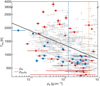 |
Fig. 16 Equilibrium temperature (Teq) vs planet density (ρp) diagram for the He I detections (blue circles) and non-detections (red crosses). The black line (drawn by-eye) indicates the hinted upper boundary for the He I detections. The coloured dashed vertical lines indicate the Earth’s density (ρ⊕; orange line at ~5.5 g cm−3), and a representative density where the puffy planet population starts (ρpuffy; blue line at ~1.3 g cm−3; Luque & Pallé 2022). All known planets with Teq and ρp determined with a precision better than 50% are marked with grey dots (data from NASA Exoplanet Archive). |
6.6 He I dependence on planetary parameters
One of the aims of the MOPYS project was also to find a relation between planetary and stellar properties that could explain, and predict, the He I detections and non-detections, but without the need to involve the strength of the signal itself. From the many explored relations and diagrams, only the equilibrium temperature (Teq) and the planet density (ρp) showed some hints of such relationship. Figure 16 presents the Teq versus ρp diagram where the information about the He I observations is encoded in the colour markers (blue circles are detections, red crosses are non-detections, and non-conclusive observations are not shown). Although both are planet properties, Teq encapsulates information about the star via the Teff and the ap/R★ parameters.
From Fig. 16, one clear result is that there are no He I detections on exoplanets with Teq ≳ 2000 K. The hottest detection at Teq ~2000 K comes from the puffy planet HAT-P-67 b. In fact, the data in Fig. 16 hint to a density/Teq upper boundary for the detections. We draw ‘by-hanď this observational limit for a better visualisation, which follows Teq ≃ −500 log10(pp) trend, approximately. If we assume that detections and non-detections are distributed randomly across the Teզ–ρp parameter space, the probability of extracting 14 non-detections from a pool of 17 detections and 36 non-detections is only 0.16%. Although it is an approximate calculation, the very low probability supports the robustness of the boundary. For planets falling above the line it is unlikely that one can detect He I, as all the inspected planets resulted in non-detections. Below that line, He I detections and non-detections are equally found.
At face value our results indicate that for high-density planets (from Earth-size to sub-Neptune-size) He I absorptions are present only in cool atmospheres. A possible interpretation is that these type of planets quickly lose any H/He atmosphere when subjected to strong stellar instellation (assuming that Teq is directly related at the population level to stellar flux). For low-density planets (gas giants) He I detection are found up to ~2000 K.
Further He I detections will confirm or disprove the observational boundary proposed here, and define its exact dependence on different planet parameters.
7 Conclusions
This work shows the first results of the MOPYS survey, a project that aims to test the predictions of atmospheric evolution theories by confronting them with observations of evaporation proxies. We present CARMENES and GIARPS high-resolution transmission spectroscopy observations of 20 exoplanets. We analysed their atmospheres searching for He I triplet absorption in the NIR, and Hα in the VIS as well. We report two new detections of the He I triplet for TOI-1268 b and TOI-2018 b, and a new Hα detection for TOI-1136 d. We also found hints of He I on HD 63433 b, and of Hα on HD 73583 b and c, which need further confirmation.
We complemented our target list with other planets from the literature with He I triplet and Hα (and Lyα for some particular planets as well) observations, for a total of 70 planets. We considered those lines as proxy of evaporation to test mass-loss theories. The main findings of our study are:
Our age distribution of evaporation detections does not favour either photo-evaporation or core-powered mass-loss as planet formation mechanisms;
We find no trend in atmospheric evaporation with stellar age. Young (<1-Gyr-old) planets do not exhibit more He I or Hα detections than older planets;
Evaporation (He I or Hα) signals are more frequent or easier to detect for planets around stellar hosts within ~ 1–3 Gyr ages;
The fraction of planets that show He I detections is much larger for K-type stars (45%) than for any other spectral type;
We find no evaporation detections of young and old planets below the radius gap, confirming rocky planets are not under extreme evaporation, at least after the first ~300 Myr;
We find hints that evaporation of puffy sub-Neptunes (Rp > 3 R⊕) happens at ages older than 1 Gyr, although the number of planets is small, and a larger sample is needed to confirm this finding;
We provide new constraints to the cosmic shoreline, by using the evaporation detections as evidences for the existence of planetary atmospheres. Our cosmic shoreline move to higher irradiation flux, reducing the parameter space of bare rocky planets.
We present the He-related dimensionless parameter Rнe/Rнill, as a new valid parameter to study the He I detections and upper limits;
All the He I detections are found in planets orbiting stars with Teff ≲ 6250 K, which is the temperature at which the Kraft Break happens.
We determine a statistically significant observational upper boundary for He I detections in the Teq versus ρp parameter space. The line decays at a rate of Teq ≃ −500 log10(ρp), approximately. Planets falling above that boundary are unlikely to show He I absorption signals.
We encourage further evaporation observations (Lyα, Hα, and He I triplet) to increase and complete the sample presented in this work. Although this work represents the biggest evaporation survey to date (specially focused on <1 Gyr-old planets), some key questions of planet formation and atmospheric evaporation remained unanswered. In particular, the detection and atmospheric characterisation of very young planets (< 100 Myr) is key for discriminating between different mass-loss processes in planetary atmospheres. It is precisely because of their age that they are the most difficult planets to analyse their atmospheres.
Acknowledgements
CARMENES is an instrument at the Centro Astronómico Hispano en Andalucía (CAHA) at Calar Alto (Almería, Spain), operated jointly by the Junta de Andalucía and the Instituto de Astrofísica de Andalucía (CSIC). The authors wish to express their sincere thanks to all members of the Calar Alto staff for their expert support of the instrument and telescope operation. CARMENES was funded by the Max-Planck-Gesellschaft (MPG), the Consejo Superior de Investigaciones Científicas (CSIC), the Ministerio de Economía y Competitividad (MINECO) and the European Regional Development Fund (ERDF) through projects FICTS-2011-02, ICTS-2017-07-CAHA-4, and CAHA16-CE-3978, and the members of the CARMENES Consortium (Max-Planck-Institut für Astronomie, Instituto de Astrofísica de Andalucía, Landessternwarte Königstuhl, Institut de Ciències de l’Espai, Institut für Astro-physik Göttingen, Universidad Complutense de Madrid, Thüringer Landesstern-warte Tautenburg, Instituto de Astrofísica de Canarias, Hamburger Sternwarte, Centro de Astrobiología and Centro Astronómico Hispano-Alemán), with additional contributions by the MINECO, the Deutsche Forschungsgemeinschaft (DFG) through the Major Research Instrumentation Programme and Research Unit FOR2544 “Blue Planets around Red Stars”, the Klaus Tschira Stiftung, the states of Baden-Württemberg and Niedersachsen, and by the Junta de Andalucía. Based on observations collected at the Centro Astronómico Hispano-Alemán (CAHA) at Calar Alto, proposals 21B-3.5-004, 22A-3.5-007, 22B-3.5-009, 23A-3.5-009, and 23B-3.5-002, operated jointly by Junta de Andalucía and Consejo Superior de Investigaciones Científicas (IAA-CSIC). We used data from the CARMENES data archive at CAB (CSIC-INTA). We acknowledge the use of the ExoAtmospheres database during the preparation of this work This work is partly supported by JSPS KAKENHI Grant Number JPJP24H00017 and JSPS Bilateral Program Number JPJSBP120249910. This paper is based on observations made with the MuSCAT2 instrument, developed by ABC, at Tele-scopio Carlos Sánchez operated on the island of Tenerife by the IAC in the Spanish Observatorio del Teide. We acknowledge financial support from the Agencia Estatal de Investigación (AEI/10.13039/501100011033) of the Ministe-rio de Ciencia e Innovación and the ERDF “A way of making Europe” through projects PID2022-137241NBC4[1:4], PID2019-109522GB-C5[1:4], PID2021-125627OB-C31, PID2022-141216NB-I00, Ariel Postdoctoral Fellowship program of the Swedish National Space Agency (SNSA), and the Centre of Excellence “Severo Ochoa” and “María de Maeztu” awards to the Instituto de Astrofísica de Canarias (CEX2019-000920-S), Instituto de Astrofísica de Andalucía (CEX2021-001131-S) and Institut de Ciències de l’Espai (CEX2020-001058-M). J.O-M. agraeix el recolzament, suport i ànims que sempre ha rebut per part de Padrina Conxa, Padrina Mercè, Jeroni, Mercè i més familiars i amics. J.0.M. gratefully acknowledge the inspiring discussions with Maite Mateu, Alejandro Almodóvar, and Joan Perelló, and the support from Guillem, Benet, and Montse. This research has made use of resources from VallAlbaida-Mallorca collaboration. J.0.M. acknowledges the contributions and patience of Jorge Terol Calvo, i molt especialment a tu, Yess. L.N. and F.L. acknowledge the support by the Deutsche Forschungsgemeinschaft (DFG, German Research Foundation) – Project number 314665159. E.K. and S.H.A. acknowledge the support from the Danish Council for Independent Research through grant no. 2032-00230B. E.N. acknowledges the support by the DFG Research Unit FOR2544 “Blue Planets around Red Stars”. S.C. acknowledges the support of the DFG priority program SPP 1992 “Exploring the Diversity of Extrasolar Planets” (CZ 222/5-1).
Appendix A Additional figures
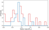 |
Fig. A.1 Histogram of He I triplet observations (detections: blue, non-detections: red) as a function of stellar mass. |
Appendix A Additional transmission spectroscopy results
B.1 K2-100 b
The resulting residual maps and TS centred in the spectral regions of the Hα and He I triplet are shown in Figure A.1. The time evolution of all the activity indices is mainly flat, and there is no evidence of strong stellar variability during the transit.
The He I triplet TS shows a flat spectrum, while the Hα TS is flat with some emission features from stellar variations in the line core during the transit. We found no significant absorption in either of the lines, and we placed a 3σ upper limit to the excess absorptions of 1.4 % and 1.3 % for Hα and He I, respectively.
K2-100 b was already observed with the InfraRed Doppler (IRD) spectrograph on the 8.2-m Subaru telescope (ℛ = 70 000; Kotani et al. 2018). Gaidos et al. (2020a) derived an EW 99% confidence detection upper limit of 5.7 mÅ. From Fig. 8 therein, we estimated an absorption depth of ~1.2%, which is consistent with the upper limit derived from the CARMENES observations.
B.2 MASCARA-2 b
Casasayas-Barris et al. (2019) already detected Hα in MASCARA-2b using CARMENES and HARPS-N observations. The Hα absorption measured with CARMENES VIS data was −0.85±0.03 %, and while combining 3 nights with HARPS-N was −0.68±0.06 %.
Here, we inspected the CARMENES NIR spectra, which were not analysed in Casasayas-Barris et al. (2019), looking for He I excess absorption. Figure A.2 presents the residual map and TS around the He I triplet. Because some telluric OH variability was still remaining in the residual map, we masked the affected regions. Despite the structure in the final TS, due to the masked regions, we found no significant planetary absorption. We computed a 3σ upper limit to the He I excess absorption of 0.5%.
B.3 V1298 Tau c
V1298 Tau planetary system is known to have transit time variations (TTVs) that can complicate the analysis of high-resolution spectroscopy observations (David et al. 2019). According to nonlinear ephemerids for the V 1298 Tau system (J. Livingston, priv. comm.), a nearly complete transit of planet c was observed the night of 5 of January 2020. Unfortunately, we missed pre-transit observations which are critical to compute a good MO and to check for stellar variability during the observations.
For this transit, the serval Hα index shows a clear decrease only from about mid-transit to egress, and an increase at the end of the observations. We did not include those last spectra in the computation of the MO spectrum, although they are plotted in the residual maps. The other serval products do not show signs of strong stellar activity (see Fig. A.2l).
The Hα residual map (Fig. A.3 left) shows a clear absorption region coincident with the serval Hα index decrease, suggesting the stellar origin of the signal. We computed the TS only with the non-affected spectra from the first half of the transit. We fitted a −1.10 ± 0.13 % feature at the Hα position, which is consistent with the 3σ upper limit derived from the nearby spectral region (1.1 %). The priors and posterior values from the fit are listed in Table B.1, and the posterior distributions are shown in Fig.B.1.
The first half of the transit in the He I NIR triplet residual map (Fig. A.3 left) shows an extended absorption region, which does not coincide in time with the Hα variability detected. In the second half of the transit, there is a vertical absorption feature in the stellar rest frame that does not follow the planetary track when we shift the spectra into the planet rest frame. This feature seems to be related to telluric residuals. We computed the TS with those unaffected spectra from the first half of the transit. The He I TS has a deep (−3.75 ± 0.12 %) and broad (1.02 ± 0.04 Å) absorption feature, which is larger than the 3σ upper limit (1.1 %). The priors and posterior values from the fit are listed in Table B.2, and the posterior distributions are shown in Fig. B.1.
To explore the origin of the Hα and He I features, we computed the TS from the unaffected spectra (start phase), the centre of the transit (centre phase), the end of the transit (end phase), and post-transit. We compare those TS with the MO spectra in Fig. B.2. The start TS from Hα and He I lines show a different behaviour from centre and end. Furthermore, the comparison between TS and MO evidences the stellar line profile variation during the observations. Therefore, we cannot confidently attribute the detected features to V1298 Tau c atmosphere. Moreover, the Hα TS in Fig. B.2 show a tiny bump at ~6563 Å which can be attributed to the star and its youth. The surprisingly large Δυ(−28.7 ± 1.1 km s−1) is another reason for not claiming the significant He I signal as a detection.
The Hα line of V1298 Tau c was previously explored by Feinstein et al. (2021) and Schlawin et al. (2021). Feinstein et al. (2021) studied with the Gemini/GRACES spectrograph the behaviour of the Hα and Ca II infrared triplet during a transit, finding significant variations of the Hα during the observations. Schlawin et al. (2021) analysed one transit looking for Hα absorption with the PEPSI spectrograph, but the observations were affected by stellar variability. Furthermore, Vissapragada et al. (2021) explored the He I triplet of planet c with the Habitable-zone Planet Finder (HPF) spectrograph, but the in-transit spectra were affected by a stellar flare. Lastly, a transit of planet c was observed with narrow-band helium filter photometry, but Vissapragada et al. (2021) did not detect the transit during the observations.
Unfortunately, our observations join the previous unsuccessful attempts to analyse the atmosphere of Vl298 Tau c. Due to the many complications that affected the observations, we adopted the absorption peaks from the Hα and He I features as upper limits of any possible planetary absorption. Our upper limits to Hα and He I excess absorption are 1.1% and 3.7%, respectively.
Observing log of the transits analysed in this work.
B.4 TOI-1431 b
Stangret et al. (2021) analysed two HARPS-N and one EXPRES transits, finding no signs of atomic or molecular absorption. A tentative detection of Hα appeared only during the first HARPS-N dataset (0.33 ± 0.07 %), but it was considered as stellar variability because it was not reproduced in the other two visits. We consider that absorption feature as an upper limit for the purpose of this work.
Here, we looked for He I excess absorption in the GIANO-B spectra from the first night of Stangret et al. (2021). The residual map and TS are shown in Fig. A.4. The TS is mainly flat and we placed a 3σ upper limit to the He I excess absorption of 0.4 %.
B.5 TOI-2048 b
Newton et al. (2022) noted that ground-based follow-up observations found a tentative transit detection ~20 min later than expected. We analysed the new available TESS data to derive updated ephemerides. The details of the photometric fit are explained in Appendix C. We refined TOI-2048 b ephemerides and planet properties (Table C.1), and confirmed the detected delay from ground-based observations. Furthermore, because TOI-2048 b does not have mass measurements, we estimated its probable mass from its radius (Wolfgang et al. 2016) to predict its semi-amplitude K★. This parameter is required for a proper measurement of the TS. We forecasted a mass of 9.4 ± 1.0 M⊕ and a K★ of 2.8 ± 0.3 m s−1. The details of all these calculations are explained in App. C as well.
The time evolution of all the activity indicators is mainly flat except for the last four Hα index points. We excluded those spectra from the MO combination, although they are plotted in the residual maps. Furthermore, we masked a region near the He I triplet because some residuals still remained after correcting the OH emission. We obtained similar results with or without applying the OH emission correction.
Hα shows a narrow absorption feature (see Fig. A.5), but we consider it too narrow to have a planetary origin (it is only one binned point). Moreover, there are emission signals around the absorption signal in the residual map, and the absorption peak is of the order of the 3σ upper limit of 1.5 %, and is difficult to distinguish from the continuum in the final TS. We found no significant absorption features around He I triplet (Fig. A.5). We placed a 3σ upper limit to the He I excess absorption of ~1 %.
B.6 HD 63433 b
The night on 1 November 2021 was cloudy until ~01:40 UT, and we could only coverthe transit partially, without pre-transitinfor-mation. The observations are a bit noisy because the exposures were set to 1 minute and we missed pre-transit observations due to bad weather conditions. Then, we observed a complete transit 1 year later, on 27 November 2022. The time evolution of all the activity indicators is mainly flat, without evidence of stellar activity during the observations in both nights. Although the RM effect was detected by Mann et al. (2020), the RM and CLV contribution to the Hα and He I triplet transmission spectra is well within the error bars of the TS (see Fig. D.1), so we decided to not correct the data from these marginal effects.
The Hα transmission spectrum from the first partial transit displays an absorption feature of  (Fig. A.6). Table D.1 shows the priors and posterior values from the fit and Fig. D.2 shows the posterior distribution. However, we did not recover that Hα absorption in our second visit, which covered the entire transit. We consider the Hα feature does not have a planetary origin. Due to the different quality around the Hα from both nights, we did not combine the two datasets. The residual map and TS for the Hα from the second transit is shown in Fig. A.6. We placed a 3σ upper limit to the Hα excess absorption of 0.4 %.
The residual maps and TS for the He I triplet from both nights separately are shown in Fig. A.6. The He I triplet was completely uncontaminated from tellurics, and both transmission spectra show some residuals from the stellar Si I line at 10830 Å. Due to the different quality of the nights, we did not combine them and focused on the second event which is less noisy. The TS presents a ~0.25 % excess absorption feature just at the expected position, but there is noise structure of similar amplitude. Finally, we adopted a conservative 3σ upper limit of 0.4 %.
Our results on the He I triplet are consistent with the previous upper limit of ~0.5 % reported by Zhang et al. (2022c). Their partial transit also showed a ~0.2% excess absorption, but they found a correlation between the stellar He I and H Paschen γ lines. We also compared the H Paschen lines with the He I line, but we could not explain the He I triplet feature as stellar line variability. Further high-S/N observations of HD 63433 b are required to confirm the interesting feature of ~0.2% around the He I triplet found in this work and Zhang et al. (2022c).
Although the study of Lyα observations is not the focus of this work, it is worth mentioning Zhang et al. (2022c) presented HST/STIS observations of HD 63433 b around the Lyα line, but no absorption was found for this planet.
B.7 HD 63433 c
The time evolution of the serval activity indicators is flat, except the Hα line index that displays a narrow peak close to mid-transit, which is also visible in the Hα residual map (Fig. A.7). Therefore, we excluded those spectra to compute the Hα TS, which is mainly flat. The Hα TS displays a too narrow absorption feature that originates only from the first half of the transit. Thus, we attributed this signal to a stellar origin rather than to absorption from the planet. We put a 3σ upper limit of 0.4 % to any possible Hα excess absorption from the planet’s atmosphere.
The He I triplet residual map and TS do not show features from the planetary atmosphere, or from stellar variability (Fig. A.7). We placed a 3σ upper limit to the He I excess absorption of 0.4 %, consistent with the previous upper limit of ~0.5% reported by Zhang et al. (2022c) with Keck/NIRSPEC.
Zhang et al. (2022c) detected an excess absorption of Lyα in one visit of HD 63433 c atmosphere with HST/STIS. However, we do not detect the evaporating atmosphere of HD 63433 c via Hα in the VIS, or the He I triplet in the NIR. Similar situation applies to, e.g. GJ 436 b where Lyα was detected (Kulow et al. 2014), but not Hα or He I triplet (Cauley et al. 2017; Nortmann et al. 2018; Villarreal D’Angelo et al. 2021).
B.8 HD 73583 b
We analysed the new TESS data to update the ephemerides on HD 73583 planetary system (see App. E) and we used them to analyse the transit of HD 73583 b observed with HARPS-N. The MO spectra was computed without the last three spectra, which show different values in the serval Hα indicator and YABI S-index. The time evolution for the other activity indicators is mainly flat.
The Hα residual map and TS are shown in Fig. A.8, where the last spectra clearly exhibit higher flux in the Hα line core. The TS shows a small absorption feature at the Hα position, which seems to come from the second half of the transit according to the residual map. The signal is −0.46±0.16 % deep (significance <3σ), and has a net shift of  km s−1. The priors and posteriors from the fit are shown in Table E.2, and the posterior distributions are plotted in Fig. E.3. However, it is hard to link that absorption to the planet atmosphere for two reasons: i) the absorption comes mostly from the second half of transit (see the residual map on Fig. A.8), and ii) the shift of the feature is in the opposite direction of the He I detection from Zhang et al. (2022b). We considered the ~0.5% absorption feature as the upper limit for Hα absorption.
Because GIANO-B was not on the telescope the night of the observations, we could not explore the He I triplet. Zhang et al. (2022b) detected an excess absorption of 0.68±0.08 % from one full and one partial transits of HD 73583 b with Keck/NIRSPEC. These observations were re-analysed in Zhang et al. (2023b) reporting a new excess absorption measurement of 0.72±0.08 %. The He I triplet signal has a blue shift, rather than the usual red-shift reported in the other He I detections.
B.9 HD 73583 c
As we mention in the previous section, the TESS photometric analysis for the HD 73583 planetary system is shown in App. E. Using the values from Barragán et al. (2022), the uncertainty on HD73583 c Tc would be 50minutes, while we now obtained a precision of ~1 min.
The time evolution of the serval Hα and dLW indicators show a peak at the beginning of the transit that extends until mid-transit. Thus, to compute the TS, we only considered the spectra from the second half of the transit. The other activity indicators show a scattered but flat time evolution. The Hα residual map and TS are shown in Fig. A.9, where the Hα variability is visible in the residual map. The TS has a small feature at the expected position. We fitted an absorption of  , and we present the prior and posterior values in Table E.3, and the posterior distributions are shown in Fig. E.3. Although the fitted absorption is significant (~3.8 σ), we consider that value as an upper limit or a tentative detection. A second transit with better S/N and no stellar activity will confirm these results.
The He I triplet residual map and TS is shown in Fig. A.9. There is no clear evidence of a planetary trace on the residual map or planetary absorption detected on the TS. We placed a 3σ upper limit to the He I excess absorption of 0.5 %.
B.10 HD 235088 b
We observed one transit of this sub-Neptune-sized planet during this project and its results were analysed in depth in Orell-Miquel et al. (2023). We detected a He I blueshifted absorption signal of −0.91 ±0.11 %, confirming the previous detection from Zhang et al. (2023b) of −0.64±0.06 % absorption. The residual maps and transmission spectra for the Hα and He I triplet are shown in Fig. A.10 (adapted from Orell-Miquel et al. 2023).
In this work we adopted the results presented in Orell-Miquel et al. (2023), where an age of 600-800 Myr was estimated for HD235088.
B.11 K2-77 b
Because K2-77 b ephemerides are based on K2 photometry, we decided to analyse the available TESS data and improve the uncertainties on Tc for this target (see App. F).
According to our results, the last spectrum from the CARMENES observations was taken during the egress, missing the post-transit coverage to compute the MO spectrum. Moreover, the pre-transit observations have low S/N due to higher airmass.
The difficulties to calculate the MO spectrum are visible in the residual maps and TS for both Hα and He I triplet lines (Fig. A.11). We could only derive broad 3σ upper limits for Hα and He I excess absorptions of 2.5 % and 2.7 %, respectively.
B.12 TOI-2046 b
We set GIARPS mode observations with similar exposure times than for HARPS-N and GIANO-B. Due to the faintness of the host star (J =10.4 mag), we used GIANO-B’s maximum time exposure of 600s for both spectrographs. The spectra have relatively low S/N around the Hα and the He I triplet. Also, the GOFIO pipeline could not properly remove the biggest telluric OH emission peak, and we decided to mask those telluric affected regions. The masked regions are far enough from the He I line to ensure that they do not affect the final results.
Hα and He I residual maps and TS are shown in Figures A.12. We only could derive very broad 3σ upper limits for Hα and He I excess absorptions of 5 % and 2.9 %, respectively.
B.13 TOI-1807 b
We analysed the newly available TESS data to derive updated ephemerids, and refine the Tc. The details of the photometric fit are explained in App. G, and our results for the planet properties are shown in Table G.1. However, we planned the observations with older ephemerides (Nardiello et al. 2022), missing part of the transit on 16 December 2022. We observed a second full transit on 23 December 2022, also with better S/N. The Hα and He I residual maps and TS for both events are shown in Figures A.13. The second visit does not show evidences of absorption features. We only used the data from the second transit to compute upper limits due to the different quality between both observations. We derived a 3σ upper limit of 0.95 % for Hα excess absorption, and an upper limit of 0.80 % for the He I triplet.
A transit of this ultra-short period (USP) Earth-like density planet was already observed with IRD, reporting an upper limit to the He I triplet EW of 4 mÅ (Gaidos et al. 2023, ~0.4 % absorption). Because our upper limit is less constraining than the previous observations, we used the results from Gaidos et al. (2023) in the discussion in Section 4.
B.14 TOI-2076 b
In this section we present the analyses and results from one CARMENES transit of TOI-2076 b observed in 2023. Previously in May 2022, we missed a transit of TOI-2076 c due to imprecise ephemerides from Hedges et al. (2021). Nowadays, the periods of TOI-2076 planets are well-constrained and refined (Osborn et al. 2022; Zhang et al. 2023b), and we could confirm that none of the three planets were transiting the night of 11 May 2022. However, we take advantage of those observations to study the behaviour of the star between epochs. The values derived from the serval activity indicators for the two datasets are consistent, and there are no differences between epochs. The levels of stellar activity of both visits are very similar and TOI-2076 b transit seems unaffected by stellar activity o variability. Due to bad weather conditions at the beginning of the night of 13 April 2023, we missed the pre-transit baseline and a very small part of the transit. Moreover, the median S/N of the in-transit spectra is lower (~60) than after transit (~90).
The TTVs of the TOI-2076 system (Osborn et al. 2022) make the scheduling of its transits complicated and increase the probability of missing part of them. Thus, we complemented our observations on 2023 with a photometric follow-up. We could not perform simultaneous observations on 13 April 2023, but we detected TOI-2076 b ingress one month after (14 May 2023). The details of the photometric analysis and their results are explained in App. J.
The Hα residual map and TS are shown in Fig. A.15. The TS close to the Hα has consistently negative values that could be considered as a planetary absorption. Although the lack of pre-transit baseline could be the origin of the signal, as for HD 63433 b transit on 1 November 2021 (App. B.6). Then, a full transit coverage is needed to confirm this tentative signal. We set a 3σ upper limit of 0.7% to Hα exoplanet absorption.
The He I triplet residual map and TS are shown in Fig. A.15. We do not detect clear evidences of He I planetary absorption. We looked for correlations of the He I NIR line with the He I D3 (5877.2 Å), and H Paschen lines, with no conclusive results. We could only put a 3σ upper limit of ~1% for any He I triplet planetary absorption.
TOI-2076 b atmosphere was already targeted looking for He I. The same partial transit was observed from the same mountain with two different 8-m telescopes with their high-resolution spectrographs. In both cases, a consistent feature was detected but there are differences in the interpretation of the signal. Zhang et al. (2023b) with Keck/NIRSPEC reported a He I detection with an excess absorption of 1.01 ±0.05 % (EW = 10.0±0.7). On the other hand, Gaidos et al. (2023) fitted a significant excess EW of 8.5± 1.4 mÅ, but their analyses did not rule out the stellar origin of the signal. Although CARMENES has the capability to detect such He I excess absorptions (e.g. Salz et al. 2018; Alonso-Floriano et al. 2019; Orell-Miquel et al. 2023), the S/N of our transit only allows us to put an upper limit at ~1%, which is at the same level of the previous detected feature. Further observations in good weather conditions are needed to firmly confirm the TOI-2076 b He I signal. For the purpose of this work, we use the positive results from Zhang et al. (2023b) in the discussion.
We also used the dataset from May 2022 to check for H/He structures around TOI-2076, recently reported in other exoplan-ets (Zhang et al. 2023c; Gully-Santiago et al. 2024). However, we obtained very similar results when we included those spectra in the analyses of TOI-2076 b Hα and He I lines.
B.15 TOI-1683 b
We scheduled three transits of TOI-1683b for the MOPYS project, one with CARMENES and two with GIARPS. CARMENES transit was stopped due to bad weather and the few taken spectra are useless for atmospheric analyses. The two other transits were observed only with GIANO-B due to problems with the GIARPS mode, and we could not observe until ingress for the first GIANO-B visit (19 September 2023).
Zhang et al. (2023b) reported an age of 500±150Myr, based on gyrochronology relations. Here, we derived a new age estimation of  Gyrbased on gyrochronology, stellar kinematics, and stellar Li I analyses, indicating that TOI-1683 is not a young star. Hence, we do not consider TOI-1683 b as a young planet. The details of our stellar age analyses are explained in Appendix K. Furthermore, we derived new ephemerides for TOI-1683 b using the available TESS data from Sectors 19, 43, and 44 in the MAST archive. The photometric analyses and results are shown in Appendix K as well.
Zhang et al. (2023b) observed one transit in bad weather conditions with Keck/NIRSPEC, and reported a He I detection of 0.84±0.17 %. Although we also observe in poor weather and seeing conditions, we do not detect a significant He I excess absorption in the individual or combined nights from GIANO-B. The residual maps and TS from the individual and combined nights are shown in Fig. A.16. We placed a 3σ upper limit from our two visits with GIANO-B to the He I excess absorption of 0.7 %, which is ~1σ consistent with Zhang et al. (2023b) detection. We use the positive detection from Zhang et al. (2023b) in the discussion.
B.16 WASP-189 b
Stangret et al. (2022) already analysed one HARPS-N and two HARPS observations finding a Hα absorption feature of −0.13±0.02%. However, because the line was affected by the RM effect, they were cautious claiming a detection. Here, we inspected the GIANO-B data taken simultaneously to those HARPS-N observations.
The Si I and He I stellar lines are not detectable in the spectra and the only visible spectral features are the H2O telluric absorption lines, which we masked in the residual map and TS, shown in Fig. A.17. Although the TS has some structure, there is no evidence of He I triplet absorption. We set a 3σ upper limit of 0.3 % to the He I absorption on WASP-189 b.
B.17 HAT-P-57 b
HAT-P-57b is an ‘adolescent’ planet ( Gyr; Hartman et al. 2015), where Stangret et al. (2022) found an Hα absorption feature (−0.7±0.2%). However, the signal is narrow compared to other Hα detections from the literature and it is surrounded by pulsations from the host star.
We analysed one archival CARMENES NIR transit to inspect the He I triplet. Although we masked some regions of strong tellurics, the residual map and TS in Fig. A.18 do not show any significant planetary absorption signal. We set a 3σ upper limit of 1 % to the planetary He I absorption.
References
- Addison, B. C., Knudstrup, E., Wong, I., et al. 2021, AJ, 162, 292 [NASA ADS] [CrossRef] [Google Scholar]
- Allan, A. P., Vidotto, A. A., Villarreal D’Angelo, C., Dos Santos, L. A., & Driessen, F. A. 2024, MNRAS, 527, 4657 [Google Scholar]
- Allart, R., Bourrier, V., Lovis, C., et al. 2018, Science, 362, 1384 [Google Scholar]
- Allart, R., Lemée-Joliecoeur, P. B., Jaziri, A. Y., et al. 2023, A&A, 677, A164 [NASA ADS] [CrossRef] [EDP Sciences] [Google Scholar]
- Alonso-Floriano, F. J., Snellen, I. A. G., Czesla, S., et al. 2019, A&A, 629, A110 [NASA ADS] [CrossRef] [EDP Sciences] [Google Scholar]
- Anderson, D. R., Temple, L. Y., Nielsen, L. D., et al. 2018, arXiv e-prints [arXiv:1809.04897] [Google Scholar]
- Attia, O., Bourrier, V., Delisle, J. B., & Eggenberger, P. 2023, A&A, 674, A120 [NASA ADS] [CrossRef] [EDP Sciences] [Google Scholar]
- Barenfeld, S. A., Carpenter, J. M., Ricci, L., & Isella, A. 2016, ApJ, 827, 142 [Google Scholar]
- Barragán, O., Aigrain, S., Kubyshkina, D., et al. 2019, MNRAS, 490, 698 [Google Scholar]
- Barragán, O., Armstrong, D. J., Gandolfi, D., et al. 2022, MNRAS, 514, 1606 [CrossRef] [Google Scholar]
- Baruteau, C., Bai, X., Mordasini, C., & Mollière, P. 2016, Space Sci. Rev., 205, 77 [CrossRef] [Google Scholar]
- Bello-Arufe, A., Cabot, S. H. C., Mendonça, J. M., Buchhave, L. A., & Rathcke, A. D. 2022, AJ, 163, 96 [NASA ADS] [CrossRef] [Google Scholar]
- Benatti, S., Damasso, M., Borsa, F., et al. 2021, A&A, 650, A66 [NASA ADS] [CrossRef] [EDP Sciences] [Google Scholar]
- Brogi, M., Giacobbe, P., Guilluy, G., et al. 2018, A&A, 615, A16 [NASA ADS] [CrossRef] [EDP Sciences] [Google Scholar]
- Brown, D. J. A., Triaud, A. H. M. J., Doyle, A. P., et al. 2017, MNRAS, 464, 810 [Google Scholar]
- Brown, T. M., Baliber, N., Bianco, F. B., et al. 2013, PASP, 125, 1031 [Google Scholar]
- Buchner, J., Georgakakis, A., Nandra, K., et al. 2014, A&A, 564, A125 [NASA ADS] [CrossRef] [EDP Sciences] [Google Scholar]
- Caballero, J. A., Guàrdia, J., López del Fresno, M., et al. 2016, SPIE Conf. Ser., 9910, 99100E [Google Scholar]
- Caldiroli, A., Haardt, F., Gallo, E., et al. 2022, A&A, 663, A122 [NASA ADS] [CrossRef] [EDP Sciences] [Google Scholar]
- Casasayas-Barris, N., Palle, E., Nowak, G., et al. 2017, A&A, 608, A135 [NASA ADS] [CrossRef] [EDP Sciences] [Google Scholar]
- Casasayas-Barris, N., Pallé, E., Yan, F., et al. 2019, A&A, 628, A9 [NASA ADS] [CrossRef] [EDP Sciences] [Google Scholar]
- Casasayas-Barris, N., Orell-Miquel, J., Stangret, M., et al. 2021a, A&A, 654, A163 [NASA ADS] [CrossRef] [EDP Sciences] [Google Scholar]
- Casasayas-Barris, N., Palle, E., Stangret, M., et al. 2021b, A&A, 647, A26 [NASA ADS] [CrossRef] [EDP Sciences] [Google Scholar]
- Castelli, F., & Kurucz, R. L. 2003, in Modelling of Stellar Atmospheres, 210, eds. N. Piskunov, W. W. Weiss, & D. F. Gray, A20 [NASA ADS] [Google Scholar]
- Cauley, P. W., Redfield, S., & Jensen, A. G. 2017, AJ, 153, 81 [NASA ADS] [CrossRef] [Google Scholar]
- Chen, G., Casasayas-Barris, N., Pallé, E., et al. 2020, A&A, 635, A171 [NASA ADS] [CrossRef] [EDP Sciences] [Google Scholar]
- Christiansen, J. L., Zink, J. K., Hardegree-Ullman, K. K., et al. 2023, AJ, 166, 248 [NASA ADS] [CrossRef] [Google Scholar]
- Claudi, R., Benatti, S., Carleo, I., et al. 2016, SPIE Conf. Ser., 9908, 99081A [NASA ADS] [Google Scholar]
- Cosentino, R., Lovis, C., Pepe, F., et al. 2012, SPIE Conf. Ser., 8446, 84461V [Google Scholar]
- Cosentino, R., Lovis, C., Pepe, F., et al. 2014, SPIE Conf. Ser., 9147, 91478C [Google Scholar]
- Czesla, S., Lampón, M., Sanz-Forcada, J., et al. 2022, A&A, 657, A6 [NASA ADS] [CrossRef] [EDP Sciences] [Google Scholar]
- Dai, F., Masuda, K., Beard, C., et al. 2023a, AJ, 165, 33 [NASA ADS] [CrossRef] [Google Scholar]
- Dai, F., Schlaufman, K. C., Reggiani, H., et al. 2023b, AJ, 166, 49 [NASA ADS] [CrossRef] [Google Scholar]
- David, T. J., Petigura, E. A., Luger, R., et al. 2019, ApJ, 885, L12 [Google Scholar]
- Dawson, R. I., & Johnson, J. A. 2018, ARA&A, 56, 175 [Google Scholar]
- Drake, G. W. 1971, Phys. Rev. A, 3, 908 [NASA ADS] [CrossRef] [Google Scholar]
- Ehrenreich, D., Bourrier, V., Wheatley, P. J., et al. 2015, Nature, 522, 459 [Google Scholar]
- El Mufti, M., Plavchan, P. P., Isaacson, H., et al. 2021, arXiv e-prints [arXiv:2112.13448] [Google Scholar]
- Espinoza, N. 2018, RNAAS, 2, 209 [Google Scholar]
- Espinoza, N., Kossakowski, D., & Brahm, R. 2019, MNRAS, 490, 2262 [Google Scholar]
- Fedele, D., van den Ancker, M. E., Henning, T., Jayawardhana, R., & Oliveira, J. M. 2010, A&A, 510, A72 [NASA ADS] [CrossRef] [EDP Sciences] [Google Scholar]
- Feinstein, A. D., Montet, B. T., Johnson, M. C., et al. 2021, AJ, 162, 213 [NASA ADS] [CrossRef] [Google Scholar]
- Feroz, F., Hobson, M. P., & Bridges, M. 2009, MNRAS, 398, 1601 [NASA ADS] [CrossRef] [Google Scholar]
- Foreman-Mackey, D., Agol, E., Angus, R., & Ambikasaran, S. 2017, AJ, 154, 220 [NASA ADS] [CrossRef] [Google Scholar]
- Fossati, L., Guilluy, G., Shaikhislamov, I. F., et al. 2022, A&A, 658, A136 [NASA ADS] [CrossRef] [EDP Sciences] [Google Scholar]
- Fuhrmeister, B., Czesla, S., Hildebrandt, L., et al. 2020, A&A, 640, A52 [NASA ADS] [CrossRef] [EDP Sciences] [Google Scholar]
- Fukui, A., Narita, N., Tristram, P. J., et al. 2011, PASJ, 63, 287 [NASA ADS] [Google Scholar]
- Fulton, B. J., & Petigura, E. A. 2018, AJ, 156, 264 [Google Scholar]
- Fulton, B. J., Petigura, E. A., Howard, A. W., et al. 2017, AJ, 154, 109 [Google Scholar]
- Fulton, B. J., Petigura, E. A., Blunt, S., & Sinukoff, E. 2018, PASP, 130, 044504 [Google Scholar]
- Gaidos, E., Mann, A. W., Rizzuto, A., et al. 2017, MNRAS, 464, 850 [NASA ADS] [CrossRef] [Google Scholar]
- Gaidos, E., Hirano, T., Mann, A. W., et al. 2020a, MNRAS, 495, 650 [Google Scholar]
- Gaidos, E., Hirano, T., Wilson, D. J., et al. 2020b, MNRAS, 498, L119 [NASA ADS] [CrossRef] [Google Scholar]
- Gaidos, E., Hirano, T., Omiya, M., et al. 2021, RNAAS, 5, 238 [NASA ADS] [Google Scholar]
- Gaidos, E., Hirano, T., Beichman, C., et al. 2022, MNRAS, 509, 2969 [Google Scholar]
- Gaidos, E., Hirano, T., Lee, R. A., et al. 2023, MNRAS, 518, 3777 [Google Scholar]
- Ginzburg, S., Schlichting, H. E., & Sari, R. 2016, ApJ, 825, 29 [Google Scholar]
- Ginzburg, S., Schlichting, H. E., & Sari, R. 2018, MNRAS, 476, 759 [Google Scholar]
- Güdel, M., Dvorak, R., Erkaev, N., et al. 2014, in Protostars and Planets VI, eds. H. Beuther, R. S. Klessen, C. P. Dullemond, & T. Henning, 883 [Google Scholar]
- Guenther, E. W., Fossati, L., & Kabath, P. 2023, arXiv e-prints [arXiv:2311.02965] [Google Scholar]
- Guilluy, G., Andretta, V., Borsa, F., et al. 2020, A&A, 639, A49 [EDP Sciences] [Google Scholar]
- Guilluy, G., Bourrier, V., Jaziri, Y., et al. 2023, A&A, 676, A130 [NASA ADS] [CrossRef] [EDP Sciences] [Google Scholar]
- Gully-Santiago, M., Morley, C. V., Luna, J., et al. 2024, AJ, 167, 142 [NASA ADS] [CrossRef] [Google Scholar]
- Gupta, A., & Schlichting, H. E. 2020, MNRAS, 493, 792 [Google Scholar]
- Haisch, Karl E., J., Lada, E. A., & Lada, C. J. 2001, ApJ, 553, L153 [Google Scholar]
- Hartman, J. D., Bakos, G. Á., Buchhave, L. A., et al. 2015, AJ, 150, 197 [NASA ADS] [CrossRef] [Google Scholar]
- Hedges, C., Hughes, A., Zhou, G., et al. 2021, AJ, 162, 54 [NASA ADS] [CrossRef] [Google Scholar]
- Hernández, J., Hartmann, L., Megeath, T., et al. 2007, ApJ, 662, 1067 [Google Scholar]
- Hirano, T., Krishnamurthy, V., Gaidos, E., et al. 2020, ApJ, 899, L13 [Google Scholar]
- Hirano, T., Gaidos, E., Harakawa, H., et al. 2024, MNRAS, 530, 3117 [NASA ADS] [CrossRef] [Google Scholar]
- Howard, W. S., Kowalski, A. F., Flagg, L., et al. 2023, ApJ, 959, 64 [NASA ADS] [CrossRef] [Google Scholar]
- Jackson, A. P., Davis, T. A., & Wheatley, P. J. 2012, MNRAS, 422, 2024 [Google Scholar]
- Kabáth, P., Chaturvedi, P., MacQueen, P. J., et al. 2022, MNRAS, 513, 5955 [CrossRef] [Google Scholar]
- Kasper, D., Bean, J. L., Oklopcic, A., et al. 2020, AJ, 160, 258 [NASA ADS] [CrossRef] [Google Scholar]
- Kausch, W., Noll, S., Smette, A., et al. 2015, A&A, 576, A78 [NASA ADS] [CrossRef] [EDP Sciences] [Google Scholar]
- Kipping, D. M. 2013, MNRAS, 435, 2152 [Google Scholar]
- Kirk, J., Alam, M. K., López-Morales, M., & Zeng, L. 2020, AJ, 159, 115 [Google Scholar]
- Kirk, J., Dos Santos, L. A., López-Morales, M., et al. 2022, AJ, 164, 24 [NASA ADS] [CrossRef] [Google Scholar]
- Koskinen, T. T., Lavvas, P., Huang, C., et al. 2022, ApJ, 929, 52 [NASA ADS] [CrossRef] [Google Scholar]
- Kotani, T., Tamura, M., Nishikawa, J., et al. 2018, SPIE Conf. Ser., 10702, 1070211 [Google Scholar]
- Kraft, R. P. 1967, ApJ, 150, 551 [Google Scholar]
- Kreidberg, L. 2015, PASP, 127, 1161 [Google Scholar]
- Krishnamurthy, V., Hirano, T., Gaidos, E., et al. 2023, MNRAS, 521, 1210 [NASA ADS] [CrossRef] [Google Scholar]
- Krolikowski, D. M., Kraus, A. L., Tofflemire, B. M., et al. 2024, AJ, 167, 79 [NASA ADS] [CrossRef] [Google Scholar]
- Kulow, J. R., France, K., Linsky, J., & Loyd, R. O. P. 2014, ApJ, 786, 132 [Google Scholar]
- Lampón, M., López-Puertas, M., Lara, L. M., et al. 2020, A&A, 636, A13 [NASA ADS] [CrossRef] [EDP Sciences] [Google Scholar]
- Lampón, M., López-Puertas, M., Czesla, S., et al. 2021a, A&A, 648, A7 [Google Scholar]
- Lampón, M., López-Puertas, M., Sanz-Forcada, J., et al. 2021b, A&A, 647, A129 [EDP Sciences] [Google Scholar]
- Lampón, M., López-Puertas, M., Sanz-Forcada, J., et al. 2023, A&A, 673, A140 [NASA ADS] [CrossRef] [EDP Sciences] [Google Scholar]
- Lendl, M., Csizmadia, S., Deline, A., et al. 2020, A&A, 643, A94 [EDP Sciences] [Google Scholar]
- Lopez, E. D., Fortney, J. J., & Miller, N. 2012, ApJ, 761, 59 [Google Scholar]
- Loyd, R. O. P., Shkolnik, E. L., Schneider, A. C., et al. 2020, ApJ, 890, 23 [NASA ADS] [CrossRef] [Google Scholar]
- Lund, M. B., Rodriguez, J. E., Zhou, G., et al. 2017, AJ, 154, 194 [Google Scholar]
- Luque, R., & Pallé, E. 2022, Science, 377, 1211 [NASA ADS] [CrossRef] [Google Scholar]
- Mallorquín, M., Béjar, V. J. S., Lodieu, N., et al. 2023, A&A, 671, A163 [NASA ADS] [CrossRef] [EDP Sciences] [Google Scholar]
- Malsky, I., Rogers, L., Kempton, E. M. R., & Marounina, N. 2023, Nat. Astron., 7, 57 [Google Scholar]
- Mann, A. W., Johnson, M. C., Vanderburg, A., et al. 2020, AJ, 160, 179 [Google Scholar]
- Mayor, M., Pepe, F., Queloz, D., et al. 2003, The Messenger, 114, 20 [NASA ADS] [Google Scholar]
- McCully, C., Volgenau, N. H., Harbeck, D.-R., et al. 2018, SPIE Conf. Ser., 10707, 107070K [Google Scholar]
- McLaughlin, D. B. 1924, ApJ, 60, 22 [Google Scholar]
- Morris, R. L., Twicken, J. D., Smith, J. C., et al. 2017, Kepler Data Processing Handbook: Photometric Analysis, Kepler Science Document KSCI-19081-002 [Google Scholar]
- Murray-Clay, R. A., Chiang, E. I., & Murray, N. 2009, ApJ, 693, 23 [Google Scholar]
- Nagel, E., Czesla, S., Kaminski, A., et al. 2023, A&A, 680, A73 [NASA ADS] [CrossRef] [EDP Sciences] [Google Scholar]
- Nardiello, D., Malavolta, L., Desidera, S., et al. 2022, A&A, 664, A163 [NASA ADS] [CrossRef] [EDP Sciences] [Google Scholar]
- Narita, N., Fukui, A., Kusakabe, N., et al. 2019, J. Astron. Telescopes Instrum. Syst., 5, 015001 [Google Scholar]
- Newton, E. R., Rampalli, R., Kraus, A. L., et al. 2022, AJ, 164, 115 [Google Scholar]
- Ninan, J. P., Stefansson, G., Mahadevan, S., et al. 2020, ApJ, 894, 97 [Google Scholar]
- Nortmann, L., Pallé, E., Salz, M., et al. 2018, Science, 362, 1388 [Google Scholar]
- Oklopcic, A. 2019, ApJ, 881, 133 [NASA ADS] [CrossRef] [Google Scholar]
- Oklopcic, A., & Hirata, C. M. 2018, ApJ, 855, L11 [CrossRef] [Google Scholar]
- Oliva, E., Origlia, L., Maiolino, R., et al. 2012, SPIE Conf. Ser., 8446, 84463T [NASA ADS] [Google Scholar]
- Oliva, E., Origlia, L., Scuderi, S., et al. 2015, A&A, 581, A47 [NASA ADS] [CrossRef] [EDP Sciences] [Google Scholar]
- Orell-Miquel, J. 2024, Supplementary material of "The MOPYS project: a survey of 70 planets in search of extended He I and H atmospheres. No evidence of enhanced evaporation in young planets" [Google Scholar]
- Orell-Miquel, J., Murgas, F., Pallé, E., et al. 2022, A&A, 659, A55 [NASA ADS] [CrossRef] [EDP Sciences] [Google Scholar]
- Orell-Miquel, J., Lampón, M., López-Puertas, M., et al. 2023, A&A, 677, A56 [NASA ADS] [CrossRef] [EDP Sciences] [Google Scholar]
- Osborn, H. P., Bonfanti, A., Gandolfi, D., et al. 2022, A&A, 664, A156 [NASA ADS] [CrossRef] [EDP Sciences] [Google Scholar]
- Owen, J. E., & Jackson, A. P. 2012, MNRAS, 425, 2931 [Google Scholar]
- Owen, J. E., & Lai, D. 2018, MNRAS, 479, 5012 [Google Scholar]
- Owen, J. E., & Wu, Y. 2013, ApJ, 775, 105 [Google Scholar]
- Owen, J. E., & Wu, Y. 2016, ApJ, 817, 107 [NASA ADS] [CrossRef] [Google Scholar]
- Owen, J. E., & Wu, Y. 2017, ApJ, 847, 29 [Google Scholar]
- Palle, E., Nortmann, L., Casasayas-Barris, N., et al. 2020a, A&A, 638, A61 [EDP Sciences] [Google Scholar]
- Palle, E., Oshagh, M., Casasayas-Barris, N., et al. 2020b, A&A, 643, A25 [EDP Sciences] [Google Scholar]
- Parviainen, H., Tingley, B., Deeg, H. J., et al. 2019, A&A, 630, A89 [NASA ADS] [CrossRef] [EDP Sciences] [Google Scholar]
- Pérez-González, J., Greklek-McKeon, M., Vissapragada, S., et al. 2024, AJ, 167, 214 [CrossRef] [Google Scholar]
- Petit dit de la Roche, D. J. M., van den Ancker, M. E., & Miles-Paez, P. A. 2020, RNAAS, 4, 231 [NASA ADS] [Google Scholar]
- Plez, B. 2012, Turbospectrum: Code for spectral synthesis, Astrophysics Source Code Library [record ascl:1205.004] [Google Scholar]
- Quirrenbach, A., Amado, P. J., Caballero, J. A., et al. 2014, SPIE Conf. Ser., 9147, 91471F [Google Scholar]
- Quirrenbach, A., CARMENES Consortium, Amado, P. J., et al. 2020, SPIE Conf. Ser., 11447, 114473C [Google Scholar]
- Rainer, M., Harutyunyan, A., Carleo, I., et al. 2018, SPIE Conf. Ser., 10702, 1070266 [Google Scholar]
- Ricker, G. R., Winn, J. N., Vanderspek, R., et al. 2015, J. Astron. Telescopes Instrum. Syst., 1, 014003 [Google Scholar]
- Rockcliffe, K. E., Newton, E. R., Youngblood, A., et al. 2023, AJ, 166, 77 [NASA ADS] [CrossRef] [Google Scholar]
- Rossiter, R. A. 1924, ApJ, 60, 15 [Google Scholar]
- Ryabchikova, T., Piskunov, N., Kurucz, R. L., et al. 2015, Phys. Scr, 90, 054005 [Google Scholar]
- Saidel, M., Vissapragada, S., Spake, J., et al. 2024, arXiv e-prints [arXiv:2404.08736] [Google Scholar]
- Salz, M., Schneider, P. C., Czesla, S., & Schmitt, J. H. M. M. 2015, A&A, 576, A42 [NASA ADS] [CrossRef] [EDP Sciences] [Google Scholar]
- Salz, M., Czesla, S., Schneider, P. C., et al. 2018, A&A, 620, A97 [NASA ADS] [CrossRef] [EDP Sciences] [Google Scholar]
- Sanz-Forcada, J., & Dupree, A. K. 2008, A&A, 488, 715 [NASA ADS] [CrossRef] [EDP Sciences] [Google Scholar]
- Sanz-Forcada, J., Micela, G., Ribas, I., et al. 2011, A&A, 532, A6 [NASA ADS] [CrossRef] [EDP Sciences] [Google Scholar]
- Schlawin, E., Ilyin, I., Feinstein, A. D., et al. 2021, RNAAS, 5, 195 [NASA ADS] [Google Scholar]
- Seager, S., & Sasselov, D. D. 2000, ApJ, 537, 916 [Google Scholar]
- Sicilia, D., Malavolta, L., Pino, L., et al. 2022, A&A, 667, A19 [NASA ADS] [CrossRef] [EDP Sciences] [Google Scholar]
- Smette, A., Sana, H., Noll, S., et al. 2015, A&A, 576, A77 [NASA ADS] [CrossRef] [EDP Sciences] [Google Scholar]
- Soubiran, C., Jasniewicz, G., Chemin, L., et al. 2018, A&A, 616, A7 [NASA ADS] [CrossRef] [EDP Sciences] [Google Scholar]
- Spake, J. J., Sing, D. K., Evans, T. M., et al. 2018, Nature, 557, 68 [Google Scholar]
- Spake, J. J., Oklopcic, A., Hillenbrand, L. A., et al. 2022, ApJ, 939, L11 [NASA ADS] [CrossRef] [Google Scholar]
- Speagle, J. S. 2020, MNRAS, 493, 3132 [Google Scholar]
- Stangret, M., Pallé, E., Casasayas-Barris, N., et al. 2021, A&A, 654, A73 [NASA ADS] [CrossRef] [EDP Sciences] [Google Scholar]
- Stangret, M., Casasayas-Barris, N., Pallé, E., et al. 2022, A&A, 662, A101 [NASA ADS] [CrossRef] [EDP Sciences] [Google Scholar]
- Stefansson, G., Li, Y., Mahadevan, S., et al. 2018, AJ, 156, 266 [NASA ADS] [CrossRef] [Google Scholar]
- Suárez Mascareño, A., Damasso, M., Lodieu, N., et al. 2021, Nat. Astron., 6, 232 [Google Scholar]
- Šubjak, J., Endl, M., Chaturvedi, P., et al. 2022, A&A, 662, A107 [NASA ADS] [CrossRef] [EDP Sciences] [Google Scholar]
- Talens, G. J. J., Justesen, A. B., Albrecht, S., et al. 2018, A&A, 612, A57 [NASA ADS] [CrossRef] [EDP Sciences] [Google Scholar]
- Van Eylen, V., Agentoft, C., Lundkvist, M. S., et al. 2018, MNRAS, 479, 4786 [Google Scholar]
- Van Eylen, V., Astudillo-Defru, N., Bonfils, X., et al. 2021, MNRAS, 507, 2154 [NASA ADS] [Google Scholar]
- Vidal-Madjar, A., Lecavelier des Etangs, A., Désert, J. M., et al. 2003, Nature, 422, 143 [Google Scholar]
- Villarreal D’Angelo, C., Vidotto, A. A., Esquivel, A., Hazra, G., & Youngblood, A. 2021, MNRAS, 501, 4383 [CrossRef] [Google Scholar]
- Vissapragada, S., Knutson, H. A., Jovanovic, N., et al. 2020, AJ, 159, 278 [Google Scholar]
- Vissapragada, S., Stefánsson, G., Greklek-McKeon, M., et al. 2021, AJ, 162, 222 [NASA ADS] [CrossRef] [Google Scholar]
- Vissapragada, S., Knutson, H. A., Greklek-McKeon, M., et al. 2022a, AJ, 164, 234 [NASA ADS] [CrossRef] [Google Scholar]
- Vissapragada, S., Knutson, H. A., Greklek-McKeon, M., et al. 2022b, AJ, 164, 234 [NASA ADS] [CrossRef] [Google Scholar]
- Vissapragada, S., Greklek-McKeon, M., Linssen, D., et al. 2024, AJ, 167, 199 [NASA ADS] [CrossRef] [Google Scholar]
- Wang, L., & Dai, F. 2018, ApJ, 860, 175 [Google Scholar]
- Wildi, F., Bouchy, F., Doyon, R., et al. 2022, SPIE Conf. Ser., 12184, 121841H [NASA ADS] [Google Scholar]
- Winn, J. N., Fabrycky, D., Albrecht, S., & Johnson, J. A. 2010, ApJ, 718, L145 [Google Scholar]
- Wolfgang, A., Rogers, L. A., & Ford, E. B. 2016, ApJ, 825, 19 [Google Scholar]
- Wright, N. J., Drake, J. J., Mamajek, E. E., & Henry, G. W. 2011, ApJ, 743, 48 [Google Scholar]
- Wyttenbach, A., Ehrenreich, D., Lovis, C., Udry, S., & Pepe, F. 2015, A&A, 577, A62 [NASA ADS] [CrossRef] [EDP Sciences] [Google Scholar]
- Yan, F., & Henning, T. 2018, Nat. Astron., 2, 714 [Google Scholar]
- Zahnle, K. 1998, in Astronomical Society of the Pacific Conference Series, 148, Origins, eds. C. E. Woodward, J. M. Shull, J. Thronson, & A. Harley, 364 [NASA ADS] [Google Scholar]
- Zahnle, K. J., & Catling, D. C. 2017, ApJ, 843, 122 [NASA ADS] [CrossRef] [Google Scholar]
- Zechmeister, M., Anglada-Escudé, G., & Reiners, A. 2014, A&A, 561, A59 [NASA ADS] [CrossRef] [EDP Sciences] [Google Scholar]
- Zechmeister, M., Reiners, A., Amado, P. J., et al. 2018, A&A, 609, A12 [NASA ADS] [CrossRef] [EDP Sciences] [Google Scholar]
- Zeng, L., Jacobsen, S. B., Sasselov, D. D., et al. 2019, PNAS, 116, 9723 [Google Scholar]
- Zhang, M., Cauley, P. W., Knutson, H. A., et al. 2022a, AJ, 164, 237 [NASA ADS] [CrossRef] [Google Scholar]
- Zhang, M., Knutson, H. A., Wang, L., Dai, F., & Barragán, O. 2022b, AJ, 163, 67 [NASA ADS] [CrossRef] [Google Scholar]
- Zhang, M., Knutson, H. A., Wang, L., et al. 2022c, AJ, 163, 68 [NASA ADS] [CrossRef] [Google Scholar]
- Zhang, M., Dai, F., Bean, J. L., Knutson, H. A., & Rescigno, F. 2023a, ApJ, 953, L25 [NASA ADS] [CrossRef] [Google Scholar]
- Zhang, M., Knutson, H. A., Dai, F., et al. 2023b, AJ, 165, 62 [NASA ADS] [CrossRef] [Google Scholar]
- Zhang, Z., Morley, C. V., Gully-Santiago, M., et al. 2023c, Sci. Adv., 9, eadf8736 [NASA ADS] [CrossRef] [Google Scholar]
Available at https://zenodo.org/records/12796052
Available at http://ia2-harps.oats.inaf.it:8000
We also acknowledge the He I observations of K2-33 b (Hirano et al. 2024), which appeared during the peer review process of the manuscript.
We also acknowledge the He I observations of TOI-1259A b (Saidel et al. 2024), which appeared during the peer review process of the manuscript.
All Tables
Transit and system parameters used to compute the transmission spectra for each planet analysed in this work.
All Figures
|
Fig. 1 Residuals maps and transmission spectra around the Hα line (top panels) and He I NIR triplet (bottom panels) lines for TOI-1136 d observations. Hα results are the combination of HARPS-N and CARMENES VIS observations. He I triplet results are from CARMENES NIR observations. Left panels: residual maps in the stellar rest frame. Time since mid-transit time (Tc) is shown on the vertical axis, wavelength is on the horizontal axis, and relative absorption is colour-coded. The dashed and dotted white horizontal lines indicate the different contacts during the transit. The dashed cyan tilted lines indicate the predicted trace of the planetary signals. The solid green vertical lines indicate the position of the OH emission telluric lines. The solid blue line indicates the position of the H2O absorption telluric line. Right panels: planet transmission spectra (TS) in the planet rest frame. We show the original data in light grey and the data binned by 0.2 Å in black. When an absorption signal is fitted, a red line and shaded region show the best Gaussian fit model with its 1σ uncertainties. The dotted cyan vertical lines indicate the Hα (top) and the He I triplet (bottom) lines positions. All the wavelengths in this figure are referenced in a vacuum. |
| In the text | |
|
Fig. 2 Transit light curve of Hα line from the combined observations of TOI-1136 d. The Hα light curve was constructed integrating the counts of the residual map in the planet rest frame around λ0 using σ (blue) and FWHM (orange) wavelength band passes from Table H.1. The vertical lines represent the different contacts during the transit. |
| In the text | |
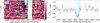 |
Fig. 3 Same as Fig. 1, but for TOI-1268 b He I triplet observations with GIANO-B. |
| In the text | |
|
Fig. 4 Transit light curve of He I triplet from TOI-1268 b detection. The He I light curve was constructed integrating the counts of the residual map in the planet rest frame around λ0 using σ (blue) and FWHM (orange) wavelength band passes from Table I.1. The vertical lines represent the different contacts during the transit. |
| In the text | |
|
Fig. 5 Same as Fig. 1, but for TOI-2018 b combined observations of Hα with HARPS-N and He I triplet with GIANO-B. |
| In the text | |
|
Fig. 6 Transit light curve of He I triplet from the combined nights of TOI-2018 b. The He I light curve was constructed integrating the counts of the residual map in the planet rest frame around λ0 using σ (blue) and FWHM (orange) wavelength band passes from Table L.3. The vertical lines represent the different contacts during the observation. |
| In the text | |
|
Fig. 7 Relationship between the observed (ṁobs) and the theoretical (ṁtheory) energy-limited mass-loss rates. We define XUV until the He I ionisa-tion range (λ = 5–504 Å). The black line indicates the fitted relationship (shown in the legend) and the shaded area the 1σ uncertainty. He I observations are coded as blue circles for detections, red crosses for non-detections, orange down-pointing triangles for non-conclusive. We did not plot the error bars of ṁtheory due to the very large uncertainties associated with the FXUV values and its calculation. Every planet has its name labelled: in black for detections and the others in grey. The two new detections presented in this work, TOI-2018 b and TOI-1268 b, are in good agreement with the predicted trend. |
| In the text | |
|
Fig. 8 Planetary radius vs stellar age diagram of evaporation (H and He I) detections (blue circles), non-detections (red crosses), and non-conclusive observations (orange down-pointing triangles). Planetary radii and stellar ages are from Table M.1. The top panel shows the summed histogram of evaporation detections (blue line) and non-detections (red line) across stellar age. The grey points represent all known planets with radius and age determined with precision better than 30% and 50%, respectively (data from NASA Exoplanet Archive). |
| In the text | |
|
Fig. 9 Equivalent width (EW) of He I detections (blue circles), non-detections (red crosses), and non-conclusive observations (orange down-pointing triangles) as functions of stellar age. The top panel shows the summed histogram of He I detections (blue line) and non-detections (red line) across stellar age bins. |
| In the text | |
|
Fig. 10 Radius-period diagrams for planets with ages ≤ 1 Gyr (top panels) and >l Gyr (bottom panels) with He I (left panels) and H (Hα or Lyα. middle panels) observations, and evaporation (combination of He I and/or H observations, right panels). Detections and non-detections are marked as blue circles and red crosses, respectively. The radius gap (Van Eylen et al. 2018) is marked as a dashed green line. The grey points represent all known planets with period and radius determined with a precision better than 25% (data from NASA Exoplanet Archive). |
| In the text | |
|
Fig. 11 Radius-mass diagrams for planets with ages <1 Gyr (top panels) and >1 Gyr (bottom panels) with He I (left panels) and H (Hα or Lyα, middle panels) observations, and evaporation (combination of He I and/or H observations, right panels). Detections and non-detections are marked as blue circles and red crosses, respectively. The solid lines are the theoretical models from Zeng et al. (2019) for Earth-like (green) and 50% H2O+50% rocky (blue) compositions. The grey points represent all known planets with mass and radius determined with a precision better than 20% (data from NASA Exoplanet Archive). |
| In the text | |
|
Fig. 12 Cosmic shoreline compared to He I observations. He I non-detections are denoted by red error bars with no marker. He I detections are circles scaled by their Rp and colour-coded by their stellar age (lateral colour bar). Instellation relative to Earth vs escape velocity (left panel) and cumulative instellation in the XUV range relative to Earth vs escape velocity (right panel) graphics. We marked the cosmic shoreline, as I ∝ υesc4, from Zahnle & Catling (2017, solid green line) and constrained from the observations (dashed black line). Planets sitting above or on the cosmic shore and with H/He detections are labelled. |
| In the text | |
|
Fig. 13 He I transmission signal strength for the planets with detections (blue circles with error bars in black) and non-detections (red down-pointing triangles in grey) as a function of the stellar FXUV (λ = 5– 504 Å) at the planet distance. We show the equivalent height of the He I atmosphere, |
| In the text | |
|
Fig. 14 Relationship between RHe/RHill and the theoretical (ṁtheory) energy-limited mass-loss rate. We define XUV until the He I ionisation range, λ∊5– 504 A. The black line indicates the fitted relationship (shown in the legend) and the dashed area the 1σ uncertainty. He I observations are coded as blue circles for detections, red crosses for non-detections, orange down-pointing triangles for non-conclusive. The colour-coding is according to the results from Sect. 6.3 (see Fig. 7). We did not plot the error bars of ṁtheory, due to the very large uncertainties associated with the FXUV values and its calculation. Every planet has its name labelled, in black for detections and the rest are in grey. |
| In the text | |
|
Fig. 15 Histogram of He I triplet observations as function of spectral types (M, K, G, F, and O, B, and A). The number of planets with detections, non-detections, and non-conclusive observations are shown as blue, red, and orange lines, respectively. We indicate the total number of inspected planets in black at the top of each column. We indicate the percentage of detections for each spectral type in blue. |
| In the text | |
|
Fig. 16 Equilibrium temperature (Teq) vs planet density (ρp) diagram for the He I detections (blue circles) and non-detections (red crosses). The black line (drawn by-eye) indicates the hinted upper boundary for the He I detections. The coloured dashed vertical lines indicate the Earth’s density (ρ⊕; orange line at ~5.5 g cm−3), and a representative density where the puffy planet population starts (ρpuffy; blue line at ~1.3 g cm−3; Luque & Pallé 2022). All known planets with Teq and ρp determined with a precision better than 50% are marked with grey dots (data from NASA Exoplanet Archive). |
| In the text | |
|
Fig. A.1 Histogram of He I triplet observations (detections: blue, non-detections: red) as a function of stellar mass. |
| In the text | |
Current usage metrics show cumulative count of Article Views (full-text article views including HTML views, PDF and ePub downloads, according to the available data) and Abstracts Views on Vision4Press platform.
Data correspond to usage on the plateform after 2015. The current usage metrics is available 48-96 hours after online publication and is updated daily on week days.
Initial download of the metrics may take a while.