| Issue |
A&A
Volume 677, September 2023
|
|
|---|---|---|
| Article Number | A56 | |
| Number of page(s) | 17 | |
| Section | Planets and planetary systems | |
| DOI | https://doi.org/10.1051/0004-6361/202346445 | |
| Published online | 05 September 2023 | |
Confirmation of an He I evaporating atmosphere around the 650-Myr-old sub-Neptune HD 235088 b (TOI-1430 b) with CARMENES
1
Instituto de Astrofísica de Canarias (IAC),
C/ Vía Láctea s/n,
38205
La Laguna, Tenerife, Spain
e-mail: jom@iac.es
2
Departamento de Astrofísica, Universidad de La Laguna (ULL),
Avd. Astrofísico Francisco Sánchez s/n,
38206
La Laguna, Tenerife, Spain
3
Instituto de Astrofísica de Andalucía (IAA-CSIC),
Glorieta de la Astronomía s/n,
18008
Granada, Spain
4
Centro de Astrobiología (CSIC-INTA), ESAC,
Camino Bajo del Castillo s/n, Villanueva de la Cañada,
28692
Madrid, Spain
5
Centro de Astrobiología (CSIC-INTA),
Carretera de Ajalvir km 4,
28850
Torrejón de Ardoz, Madrid, Spain
6
Institut für Astrophysik und Geophysik, Georg-August-Universität,
Friedrich-Hund-Platz 1,
37077
Göttingen, Germany
7
Thüringer Landessternwarte Tautenburg,
Sternwarte 5,
07778
Tautenburg, Germany
8
Department of Space, Earth and Environment, Chalmers University of Technology,
412 96
Gothenburg, Sweden
9
Landessternwarte, Zentrum für Astronomie der Universität Heidelberg,
Königstuhl 12,
69117
Heidelberg, Germany
10
Centro Astronómico Hispano en Andalucía, Observatorio de Calar Alto, Sierra de los Filabres,
04550
Gérgal, Almería, Spain
11
Astrobiology Center,
2-21-1 Osawa, Mitaka,
Tokyo
181–8588, Japan
12
Max-Planck-Institute für Astronomie,
Königstuhl 17,
69117
Heidelberg, Germany
13
Department of Multi-Disciplinary Sciences, Graduate School of Arts and Sciences, The University of Tokyo,
3-8-1 Komaba, Meguro,
Tokyo
153–8902, Japan
14
Department of Astronomy, Graduate School of Science, The University of Tokyo,
7-3-1 Hongo, Bunkyo-ku,
Tokyo
113-0033, Japan
15
Universitäts-Sternwarte, Ludwig-Maximilians-Universität München,
Scheinerstrasse 1,
-81679
München, Germany
16
Exzellenzcluster Origins,
Boltzmannstrasse 2,
85748
Garching, Germany
17
Departamento de Física de la Tierra y Astrofísica & IPARCOSUCM (Instituto de Física de Partículas y del Cosmos de la UCM), Facultad de Ciencias Físicas, Universidad Complutense de Madrid,
28040
Madrid, Spain
18
Komaba Institute for Science, The University of Tokyo,
3-8-1 Komaba, Meguro,
Tokyo
153-8902, Japan
19
Institut de Ciències de l’Espai (ICE, CSIC),
Campus UAB, Can Magrans s/n,
08193
Bellaterra, Barcelona, Spain
20
Institut d’Estudis Espacials de Catalunya (IEEC),
08034
Barcelona, Spain
21
Hamburger Sternwarte,
Gojenbergsweg 112,
21029
Hamburg, Germany
22
Osservatorio Astronomico di Padova,
Vicolo dell’Osservatorio 5,
35122
Padova, Italy
23
Department of Astronomy, University of Science and Technology of China,
Hefei
230026, PR China
Received:
17
March
2023
Accepted:
20
June
2023
HD 235088 (TOI-1430) is a young star known to host a sub-Neptune-sized planet candidate. We validated the planetary nature of HD 235088 b with multiband photometry, refined its planetary parameters, and obtained a new age estimate of the host star, placing it at 600–800 Myr. Previous spectroscopic observations of a single transit detected an excess absorption of He I coincident in time with the planet candidate transit. Here, we confirm the presence of He I in the atmosphere of HD 235088 b with one transit observed with CARMENES. We also detected hints of variability in the strength of the helium signal, with an absorption of −0.91 ± 0.11%, which is slightly deeper (2σ) than the previous measurement. Furthermore, we simulated the He I signal with a spherically symmetric 1D hydrodynamic model, finding that the upper atmosphere of HD 235088 b escapes hydrodynamically with a significant mass loss rate of (1.5−5) × 1010 g s−1 in a relatively cold outflow, with T = 3125 ±375 K, in the photon-limited escape regime. HD 235088 b (Rp = 2.045 ± 0.075 R⊕) is the smallest planet found to date with a solid atmospheric detection – not just of He I but any other atom or molecule. This positions it a benchmark planet for further analyses of evolving young sub-Neptune atmospheres.
Key words: planets and satellites: atmospheres / stars: individual: HD 235088 / planets and satellites: individual: HD 235088 b / techniques: photometric / techniques: spectroscopic
© The Authors 2023
 Open Access article, published by EDP Sciences, under the terms of the Creative Commons Attribution License (https://creativecommons.org/licenses/by/4.0), which permits unrestricted use, distribution, and reproduction in any medium, provided the original work is properly cited.
This article is published in open access under the Subscribe to Open model. Subscribe to A&A to support open access publication.
1 Introduction
Along with their stars, planets evolve and change over time. During their early stages of formation, they suffer severe changes in their physical and orbital properties due to internal and external forces (Baruteau et al. 2016). Our knowledge of the predominance and timescales of these changes is limited and a greater number of atmospherically characterized planets is needed to constrain formation and evolution models (Dawson & Johnson 2018; Owen & Lai 2018; Tinetti et al. 2018). In this context, the study of planets at early stages of evolution is crucial for a better comprehension of different processes, such as planet formation and migration, inflation and evaporation of the primary atmospheres of rocky-core planets (Owen & Wu 2017), and the formation of the “radius gap” in the radius distribution of small planets (1–4R⊕; Fulton et al. 2017; Fulton & Petigura 2018).
Stars that host young planets are particularly useful because some of their planets are predicted to have not yet lost their extended H/He-rich primordial atmospheres. The space missions Kepler (Borucki et al. 2010), K2 (Howell et al. 2014), and Transiting Exoplanet Survey Satellite (TESS; Ricker et al. 2015) have discovered several transiting young planets orbiting <1 Gyr-old stars, such as K2-33b (David et al. 2016), as well as the V1298 Tau (David et al. 2019) and AU Mic systems (Plavchan et al. 2020). These young planets are interesting targets to study, but they are also extremely challenging to analyze due to the intrinsic stellar variations of their young host stars (Palle et al. 2020b; Benatti et al. 2021).
Moreover, the study of possible evaporating atmospheres of the young mini Neptune population is of special interest in helping identify the origin of the “radius gap”. That is the case for the HD 63433 system (Zhang et al. 2022b), HD 73583 b (TOI-560b, Zhang et al. 2022a), TOI-1683.01, HD235088.01 (TOI-1430.01), and TOI-2076 b (Zhang et al. 2022a, 2023). Two observations with Keck/NIRSPEC spectrograph robustly confirmed the presence of He I in the atmosphere of HD 73583 b. The He I detections for TOI-1683.01, HD 235088.01, and TOI-2076 b were made with single-transit observations. The same partial transit of TOI-2076 b was also observed from the same mountain with the InfraRed Doppler (IRD) spectrograph by Gaidos et al. (2023). Both analyses got a similar result of an He I excess absorption of ~1% that persisted for a short time after the egress. However, they differ in terms of the interpretation of the feature: Zhang et al. (2023) claimed the signal to be a planetary absorption, while Gaidos et al. (2023) attributed it to stellar variability.
In this work, we derive stellar parameters for HD 235088 using a high signal-to-noise (S/N) spectrum from the CARMENES spectrograph. We obtain a new age estimation for this young K-type star and validate HD 235088 b (TOI-1430 b) as a planet using multi-color photometry. With CARMENES high-resolution spectra, we confirm the previous detection of He I and, by analysing this He(23S) signal, we study the hydrodynamical escape of this planet and derive the temperature and mass-loss rate of its upper atmosphere.
2 Observations and data analysis
2.1 CARMENES observations and analysis
A single transit of the planet candidate HD 235088.01 was observed with the CARMENES1 (Quirrenbach et al. 2014, 2020) spectrograph located at the Calar Alto Observatory, Almería, Spain, on the night of 6 August 2022. CARMENES has two spectral channels: the optical channel (VIS), which covers the wavelength range of 0.52–0.96 µm with a resolving power of ℛ = 94 600, and the near-infrared channel (NIR), which covers 0.96–1.71 µm with a resolving power of ℛ = 80 400. We observed the target with both channels simultaneously and collected a total of 44 spectra of 5 min exposure time, with 28 of them between the first (T1) and fourth (T4) transit contacts. We obtained a median S/N of 72 around the Hα line and of 86 around the He I triplet.
Fiber A was used to observe the target star, while fiber B was placed on sky, separated by 88 arcsec in the east-west direction. The observations were reduced using the CARMENES pipeline caracal (Caballero et al. 2016) and both fibers were extracted with the flat-optimized extraction algorithm (Zechmeister et al. 2014). We also processed the spectra with serval2 (Zechmeister et al. 2018), which is the standard CARMENES pipeline to derive the radial velocities (RVs) and several activity indicators: the chromatic radial velocity index (CRX) and the differential line width (dLW), as well as the Hα, Na I D1 and D2, and Ca II IRT line indices.
We corrected the VIS and NIR spectra from telluric absorptions with molecfit (Smette et al. 2015; Kausch et al. 2015). We analyzed the spectroscopic observations via the well-established transmission spectroscopy technique (e.g. Wyttenbach et al. 2015; Casasayas-Barris et al. 2017). We computed the Ha transmission spectra (TS) following the standard procedure. However, because there are OH emission lines from the Earth’s atmosphere close to the He I triplet lines, we applied an extra step before computing the He I TS. First, we planned the observations to avoid a complete overlap or superposition of the OH telluric lines and the He I planetary trace. We corrected the fiber A spectra from OH telluric emission using fiber B information, which is used to generate an OH emission model for correcting the science spectra. This methodology is based in previous He I studies with CARMENES (Nortmann et al. 2018; Salz et al. 2018; Alonso-Floriano et al. 2019; Palle et al. 2020a; Casasayas-Barris et al. 2021; Czesla et al. 2022). In particular, we followed the procedure previously applied in Orell-Miquel et al. (2022). Figure D.1 compares our prediction for the telluric contamination of the He I triplet lines with the real observations.
2.2 X-ray observations and planetary irradiation
We used XMM-Newton archival observations of HD 235088 (PI M. Zhang) to calculate the X-ray luminosity of the star. The star was observed on 7 July 2021. We reduced the data following standard procedures and used the three EPIC detectors to extract a spectrum for each of them, simultaneously fitting them with a two-temperatures coronal model, using the ISIS package (Houck & Denicola 2000) and the Astrophysics Plasma Emission Database (APED; Foster et al. 2012) v3.0.9. A value of interstellar medium (ISM) absorption H column density of 1 × 1019 cm−3 was adopted, consistent with the fit to the overall spectrum, and the distance to the source. The resulting model has log  ,
,  ;
;  ,
,  ; and abundances [Fe/H] = −0.24 ± 0.17 and
 ![$\left[ {{{{\rm{Ne}}} \mathord{\left/ {\vphantom {{{\rm{Ne}}} {\rm{H}}}} \right. \kern-\nulldelimiterspace} {\rm{H}}}} \right] = 0.17_{ - 0.69}^{ + 0.28}$](/articles/aa/full_html/2023/09/aa46445-23/aa46445-23-eq5.png) . An X-ray luminosity LX, in the energy range of 0.12−2.48 keV (λ = 5− 100 Å), of (1.89 ± 0.07)× 1028 erg s−1 was calculated. We extrapolated the coronal model towards transition region temperatures, following Sanz-Forcada et al. (2011), to determine the expected EUV stellar emission. We calculate
. An X-ray luminosity LX, in the energy range of 0.12−2.48 keV (λ = 5− 100 Å), of (1.89 ± 0.07)× 1028 erg s−1 was calculated. We extrapolated the coronal model towards transition region temperatures, following Sanz-Forcada et al. (2011), to determine the expected EUV stellar emission. We calculate  and
and  for the EUV spectral ranges 100–920 Å and 100–504 Å, respectively. Our X-ray flux is ~30% lower than the value calculated by Zhang et al. (2023), likely related to the spectral fitting process (we include the Ne abundance in the fit, and they assumed no ISM absorption, M. Zhang 2023, priv. comm.). Zhang et al. (2023) report also the incident flux (27 000 erg s−1 cm−2) in the range λλ1230–2588 Å (defined as MUV in their work), after the modeling of the stellar emission that was then scaled up to match the observed flux in the XMM-Newton Optical Monitor (OM) filters UVW2 (λλ 2120 ± 500 Å) and UVM2 (λλ 2310 ± 480 Å). We find an excellent agreement between our modelled SED and the observed count rate in these two filters. However these filters have anon-negligible sensitivity at longer wavelengths. We must remark that the SED of a late-type star, as in our case, yields a ~90% result for the count rate in the filter actually coming from longer wavelengths than the nominal band-pass (see Appendix A). Thus, scaling the MUV level based on the photometry of the UV filters on board XMM-Newton must be taken with care for this type of star. In any case, our model (see Sect. 6) indicates an incident flux in the MUV range of 13 300 erg s−1 cm−2, without scaling, based on the OM flux.
2.3 TESS observations
Listed as TIC 293954617 in the TESS Input Catalog (TIC; Stassun et al. 2018), HD 235088 was observed by TESS in 2-min short-cadence integrations in Sectors 14–16, 41, and 54–56. In particular, the transit studied in this work was simultaneously observed by TESS and CARMENES in Sector 55.
We fit all the TESS simple aperture photometry (SAP; Morris et al. 2017), which is publicly available at the Mikulski Archive for Space Telescopes (MAST3), using juliet4 (Espinoza et al. 2019) to refine the central time of transit (t0) and other planetary parameters, such as the orbital period and the planetary radius. Juliet is a python library based on other public packages for transit light curve (batman, Kreidberg 2015) and GP (celerite, Foreman-Mackey et al. 2017) modelling, which uses nested sampling algorithms (dynesty, Speagle 2020; MultiNest, Feroz et al. 2009; Buchner et al. 2014) to explore the parameter space. In the fitting procedure, we adopted a quadratic limb-darkening law with the (q1,q2) parameterization introduced by Kipping (2013), and we considered the uninformative sample (r1,r2) parameterization introduced in Espinoza (2018) to explore the impact parameter of the orbit (b) and the planet-to-star radius ratio (p = Rp/R★) values. According to the flux contamination exploration in Zhang et al. (2023), we can safely fix the dilution factor to 1. Furthermore, the TESS apertures used to compute each sector light curve only include our target star (see Fig. B.1). The results from the TESS data analysis are presented in Sect. 5.1.
2.4 MuSCAT2 observations and data reduction
We observed a full transit of HD 235088.01 on 23 June 2021 with the multi-color imager MuSCAT2 (Narita et al. 2019), mounted on the Carlos Sánchez Telescope (TCS) at Teide Observatory (OT). MuSCAT2 obtained simultaneous photometry in four independent CCDs in the g, r, i, and zs photometric bands, with an exposure time setting of 5 s for all CCDs. We performed the data reduction, and the aperture photometry using the MuSCAT2 pipeline described by Parviainen et al. (2020). The multi-color lightcurves (Appendix C) were computed through a global optimization that accounts for the transit and baseline variations simultaneously, using a linear combination of covariates.
3 Stellar characterization
In this section, we revise the planet host star parameters taking advantage of the high-S/N co-added spectrum from serval and other available photometric data. Table 1 compiles the stellar parameters derived in this work, and from the literature.
3.1 Stellar parameters
To determine the bolometric luminosity of HD 235088, we first built the star’s photometric spectral energy distribution (SED) using broad- and narrow-band photometry from the literature. The stellar SED is shown in Fig. 1 including the Johnson UBVR photometry (Ducati 2002), the ugriz data from the Sloan Digital Sky Survey (York et al. 2000), Gaia Early Data Release 3 and Tycho photometry (Høg et al. 2000; Gaia Collaboration 2022), the Two Micron All Sky Survey (2MASS) near-infrared JHKS photometry (Skrutskie et al. 2006), the Wide-field Infrared Survey Explorer (WISE) W1, W2, W3, and W4 data (Wright et al. 2010), the AKARI 8-µm flux (Matsuhara et al. 2006), and the optical multi-photometry of the Observatorio Astrofísico de Javalambre (OAJ), Physics of the Accelerating Universe Astro-physical Survey (JPAS), and Photometric Local Universe Survey (JPLUS) catalogs. All of this photometric information is accessible through the Spanish Virtual Observatory (Bayo et al. 2008). In total, there are 90 photometric data points defining the SED of HD 235088 between 0.30 and ~25 µm. The OAJ/JPAS data cover very nicely the optical region in the interval 0.40–0.95 µm with a cadence of one measurement per 0.01 µm. In Fig. 1, the effective wavelengths and widths of all passbands were taken from the Virtual Observatory SED Analyzer database (Bayo et al. 2008). The Gaia trigonometric parallax was employed to convert all observed photometry and fluxes into absolute fluxes. The SED of HD 235088 clearly indicates its photospheric origin since there are no obvious mid-infrared flux excesses up to 25 µm.
We integrated the SED displayed in Fig. 1 over wavelength to obtain the absolute bolometric flux (Fbol) using the trapezoidal rule. The Gaia G-band flux was not included in the computations because the large passband width of the filter encompasses various redder and bluer filters. We then applied Mbol = −2.5 log Fbol − 18.988 (Cushing et al. 2005), where Fbol is in units of W m−2, to derive an absolute bolometric magnitude Mbol = 5.846 ± 0.016 for HD 235088, from which we obtained a bolometric luminosity of L = 0.3609 ± 0.0052 L⊙. The quoted error bar accounts for the photometric uncertainties in all observed bands and the trigonometric distance error, although photometry contributes most to the luminosity error. The contribution of fluxes at bluer and redder wavelengths not covered by the photometric observations to the stellar bolometric flux is less than 1%.
Then, we computed Teff, log ɡ, [Fe/H], and total line broadening (Vbroad; see Brewer et al. 2016) by means of the STEPARSYN code5 (Tabernero et al. 2022). The STEPARSYN code is a python implementation of the spectral synthesis method that uses the emcee MCMC sampler to infer the stellar atmospheric parameters. To perform the spectral synthesis, we employed a grid of synthetic spectra computed with the Turbospectrum (Plez 2012) radiative transfer code and the MARCS stellar atmospheric models (Gustafsson et al. 2008). The spectral synthesis employed atomic and molecular data gathered from the Gaia-ESO (GES) line list (Heiter et al. 2021). To determine the stellar parameters, we fit a selection of Fe I,II lines that are well suited to analyzing FGKM stars (Tabernero et al. 2022). Using STEPARSYN, we computed the following stellar atmospheric parameters: Teff = 5037 ± 14 K, log ɡ = 4.63 ± 0.02 dex, [Fe/H] = −0.01 ± 0.02 dex, and Vbroad = 2.89 ± 0.03 km s−1. Regarding its spectral type, the spectrum of HD 235088 is highly similar to that of HD 166620, which in turn was analyzed by Marfil et al. (2020) with exactly the same CARMENES configuration as in our observations. In all, HD 166620 is a well investigated K2 V standard star with Teff = 5039 ± 85 K and log ɡ = 4.66 ± 0.21 dex (see Marfil et al. 2020), compatible at the 1σ-level to those of HD 235088 (e.g. Johnson & Morgan 1953; Noyes et al. 1984; Nordström et al. 2004).
The radius of HD 235088 can be obtained from the Stefan-Boltzmann law that relates bolometric luminosity, effective temperature (Teff), and stellar size. From the spectral fitting of the CARMENES data, HD235088’s Teff is determined to be 5037 ± 14 K. Therefore, we estimate a radius of  , where the quoted error accounts for the luminosity uncertainty and an increased ±50 K error in temperature (the latter accounts for the STEPARSYN error and possible systematics not included in the spectral fitting analysis, e.g. different model atmospheres). This radius determination is independent of any evolutionary model and depends only on the distance (well known with Gaia), the bolometric luminosity (well determined), and the model atmospheres used to fit the observed spectra.
The mass of HD 235088 can be derived following empirical mass–luminosity relationships. Fernandes et al. (2021) used masses and radii of eclipsing binaries with FGK main-sequence components to obtain a reliable mass-radius relation, from which we inferred a mass of  for our star (by adopting a solar chemical composition).
Stellar parameters of HD 235088.
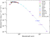 |
Fig. 1 Photometric spectral energy distribution of HD 235088 (circles) from 0.3 through ~25 µm. A black-body source with a temperature of 5050 K (solid line) is added for the sole purpose of demonstrating that all fluxes are photospheric in origin and there are no infrared flux excesses at long wavelengths. Vertical error bars denote flux uncertainties and horizontal error bars account for the width of the photometric passbands. |
3.2 Stellar rotation and age determination
Zhang et al. (2023) computed a rotational period (Prot) of 5.79 ± 0.15 days from a Lomb-Scargle periodogram of TESS SAP data and estimated an age of 165 ± 30 Myr using gyrochonologic relations. Maldonado et al. (2022) derived a similar Prot using TESS data (6.14 d), but of 12.8–14 d with STELLA and REM photometric data. However, they estimated a significantly older age of 600 Myr for HD 235088.
Here, we used seven sectors of TESS SAP data to derive a Prot of 12.0 ± 0.4 days (see Sect. 5.1 for details), which is consistent with the maximum peak at ~ 11.8 days from the computed generalized Lomb-Scargle periodogram (Zechmeister & Kürster 2009; see Fig. D.2) and with the X-ray luminosity we measured, according to the relations in Wright et al. (2011). Quantitatively, we estimated HD 235088’s age using gyrochronology with the relations presented in Mamajek & Hillenbrand (2008, Eqs. (12)–(14), the parameters from Table 10) and Schlaufman (2010, and Eq. (1)), also used in Zhang et al. (2023). We obtained ages of  Myr and
  Myr, respectively. Figure 2 shows the distribution of rotation periods as a function of color G-J for different young clusters. Qualitatively, the age of HD 235088 is consistent with the sequences of Praesepe, Hyades, and NGC 6811, that is, between 590 and 1000 Myr. Moreover, from the relation between the age for young stars and the coronal X-ray emission (Mamajek & Hillenbrand 2008, Eq. (A.3)) and using the LX derived in Sect. 2.2, we obtained
  Myr for HD 235088. Another age indicator that is commonly used is the atmospheric absorption of Li I 6709.61 Å. We looked for Li I in HD 235088 in the co-added spectrum generated by serval from the CARMENES spectra, but no clear Li I feature appeared. Therefore, we set an upper limit at 3σ of 3 mÅ, indicating that the star is not younger than the Hyades or Praesepe (~650 Myr; Fig. 3), namely, the Li I EW is not compatible with the age proposed by Zhang et al. (2023, 165 ±30 Myr). Lastly, we calculated the UVW galactocentric space velocities (Johnson & Soderblom 1987) of HD 235088 using Gaia astrometry and systemic velocity (γ) to determine if the object shares kinematics properties with known clusters, moving groups, or associations. The UVW velocities of HD 235088 are consistent with the young disk and, more particularly, with the Hyades supercluster (Fig. 4) which probably indicates its belonging to this supercluster. However, to prove its Hyades supercluster membership a more detailed study must be carried out. From the UVW velocities, we estimated an age of 600–800 Myr (Brandt & Huang 2015; Lodieu et al. 2018) which is consistent with the age reported by Maldonado et al. (2022), the rotation period, the X-ray emission, and the value we adopted forHD235088.
4 Validation of the planet candidate
We used the multi-color transit analysis approach described in Parviainen et al. (2019, 2020) to validate HD 235088.01 as a planet. The approach uses PyTransit (Parviainen 2015) to model the TESS photometry with the ground-based multi-color transit photometry to estimate the degree of flux contamination from possible unresolved sources inside the TESS photometric aperture. The contamination estimate yields a robust radius ratio estimate for the transiting planet candidate that accounts for any possible third light contamination allowed by the photometry. Combining the robust radius ratio with the stellar radius gives an absolute radius estimate of the planet candidate and if this absolute radius can be securely constrained to be smaller than the minimum brown dwarf radius limit (~0.8,RJ; Burrows et al. 2011), the planet candidate can be considered as a bona fide transiting exoplanet. This approach has been used several times in the literature to validate or reject planet candidates orbiting faint stars (Parviainen et al. 2020, 2021; Esparza-Borges et al. 2022; Murgas et al. 2022; Morello et al. 2023).
Our analysis, which combines the TESS and ground-based MuSCAT2 light curves, gives a robust radius estimate of  . This estimate can be considered the most reliable radius estimate for the transiting object when assuming that the TESS aperture could contain flux contamination from an unknown (unresolved) source and is consistent with the radius estimate derived from TESS photometry (Rp = 2.045 + 0.075 R⊕). The radius estimate is significantly below the brown dwarf radius limit of 0.8 RJ, and, thus, we validate HD 235088.01 as a sub-Neptune-sized object HD 235088 b. Furthermore, this analysis rules out a significant flux contamination from an unresolved source of a different spectral type than the host and, thus, the basic radius obtained with that assumption can be safely adopted as the planet’s radius.
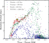 |
Fig. 2 Rotation period distribution as a function of color G-J for the Pleiades (~125 Myr; Rebull et al. 2016), Praesepe (~590 Myr; Douglas et al. 2017), Hyades (~650 Myr; Douglas et al. 2019) and NGC 6811 (~1000 Myr; Curtis et al. 2019) clusters. The gold star represents HD 235088. |
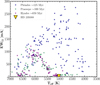 |
Fig. 3 Equivalent width distribution of Li I as a function of the effective temperature for the Pleiades (~125 Myr; Bouvier et al. 2018), Praesepe (~590 Myr), and Hyades (~650 Myr; Cummings et al. 2017). The gold triangle represents HD 235088. |
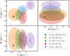 |
Fig. 4 UVW velocity diagram for HD 235088 (gold star). The members of the Castor moving group, Hyades supercluster (Hs), IC 2391 supercluster, Local Association (LA), and Ursa Major group (UMa) from Montes et al. (2001) are included. The ellipses represent the 3σ values of the UVW for each Young Moving Group. HD 235088 agrees with the Hyades supercluster. |
5 Results
5.1 Refinement of the planetary parameters
We refined the properties of the HD 235088 system fitting with juliet the available TESS SAP photometric data. We added to the transiting model a celerite GP with quasi-periodic kernel to account for the photometric variability of young star. We adopted the stellar parameters derived in Sect. 3.1 and presented in Table 1. The fitted parameters with their prior and posterior values, and the derived parameters for HD 235088 b are shown in Table 2. The TESS data along with the best transiting and GP models are shown in Fig. B.2, and HD 235088 b phase folded photometry is shown in Fig. 5.
We could improve the ephemeris and properties of HD 235088 b with the new TESS data, deriving a radius of Rp = 2.045 + 0.075 R⊕.·Moreover, the hyperparameter  accounts for the periodicities in the photometric variation, which are expected to come from the stellar rotation of the young host star. We obtained
  days, therefore, we adopt the
  value as HD 235088’s Prot. In Sect. 3.2, we computed with the generalized Lomb-Scargle periodogram method a consistent periodicity (~11.8 days, see Fig. D.2).
Some values needed to compute the transmission spectra come from the planetary mass measurement, which is still not available for our target at the time of writing. We used the information, and predicted mass (~7 ± 2 M⊕) from Zhang et al. (2023) to estimate a semi-amplitude K⋆ of ~2.5 m s−1.
Planetary parameters for HD 235088 b.
5.2 Stellar activity analysis
Before computing the TS of the Hα and He I lines, we looked for stellar activity during the observations, which could compromise or challenge the detection of planetary signals, taking advantage of the simultaneous TESS observations to the CARMENES data. However, because HD 235088 b’s transit is shallow, and HD 235088 is a young star, TESS data from a single transit do not have enough quality to clearly see if HD 235088 b passed in front of active regions or spots. There is only a ~20 min event close to mid-transit with higher flux than expected in transit, but that level of variation is consistent with the photometric variations detected in other regions of the TESS light curve.
We also checked the time evolution of the serval activity indicators during the observations and constructed the light curve of several stellar lines (all the wavelengths are given in vacuum), namely: He I D3 (5877.2 Å), H Paschenβ (Pa-β, 12821.6 Å), H Paschen γ (Pa-γ, 10941.1 Å), and H Paschen δ (Pa-δ, 10052.1 Å). The time evolution of these lines are shown in Fig. D.4. They are mainly flat except for the serval Hα index, which exhibits a strange behaviour just at the beginning of the transit. The Hα index increases smoothly, coincident with the ingress time, and then decreases at about after mid-transit. However, the He I D3 light curve is stable during the observations without evidence of fluctuations, suggesting that He I lines were not extremely affected by the Hα variability. This is consistent with the He I line being significantly less variable than the Hα line in the overall M dwarf sample observed by CARMENES (Fuhrmeister et al. 2020).
Because we used fiber B to monitor the sky, there were no simultaneous Fabry-Pérot calibrations during the observations. Thus, the expected amplitude of ~1 m s−1 for HD 235088 b’s Rossiter-McLaughlin effect is below the uncertainties of the measured RVs.
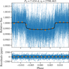 |
Fig. 5 HD 235088 TESS photometry (blue dots with error bars) phase-folded to the period, P, and central time of transit, t0, (shown above each panel, t0 units are BJD – 2 457 000) derived from the juliet fit. The black line is the best transit model for HD 235088 b. Orange points show binned photometry for visualization. The GP model was removed from the data. |
5.3 Hα and He I transmission spectra
Figure 6 (top) shows the residual map and TS around the Hα line. The residual map displays absorption coincident in time with the Hα line index feature. To avoid the affected spectra by Hα variability, we computed the Hα TS without these spectra. We only included the spectra from the second half of the transit in the calculation of the TS. The Hα TS (Fig. 6 top right) is mainly flat without a clear planetary absorption signal. We could only set an upper limit to Hα excess absorption of ~0.9%, which is computed as three times the root mean square of the TS near the line of interest.
The He I triplet residual map in Fig. 6 (bottom) shows an absorption region only during the transit, and consistent with the expected location of the planetary trace. From Sect. 5.2, we conclude that there is no evidence of strong contamination of the He I lines. Thus, the TS shown in the bottom right panel in Fig. 6 was computed from all the spectra taken fully in-transit, between the first and fourth contacts. The TS shows a clear absorption feature from the two strongest lines of the He I NIR triplet.
We fit the He I signal with a Gaussian profile, sampling from the parameter posterior distributions using the MultiNest algorithm (Feroz et al. 2009) via its python implementation PyMultinest (Buchner et al. 2014). We used uniform priors for the excess absorption between ±3%, and the central position (λ0) from 10 830 Å to 10 835 Å. Table D.1 summarizes the priors and posteriors from the nested sampling fit, and other derived properties as well. Figure D.3 displays the posterior corner plot of the distributions. We obtained an He I triplet absorption signal of −0.91 ± 0.11%, with an equivalent width of 9.5 ± 1.1 mÅ and significantly blue-shifted (−6.6 ± 1.3 km s−1).
Our absorption is deeper, but consistent at the 2σ-level with the previous detection with Keck/NIRSPEC reported by Zhang et al. (2023; depth −0.64 ± 0.06%, equivalent width 6.6 ± 0.5 mÅ, and blue shift −4.0 ± 1.4 km s−1). If we interpret the mild tension between the two values of the absorption depth as variability, it could be shown to originate from the stellar activity. The stellar activity revealed in our analysis of the Hα line could increase the XUV stellar flux, increasing the population of the He(23S) level. Zhang et al. (2023) did not present a study of the stellar activity in other than the He(23S) lines during their observations, preventing us from examining whether the different He(23S) signals are caused by the stellar variability between the two transits. Keck/NIRSPEC Y band covers from 0.946–1.130 µm, in which there are two lines of the H Paschen series: Pa-γ (10 941.1 Å), and Pa-δ (10 052.1 Å). The light curves of the stellar Pa-γ, Pa-δ, and Pa-β as well, are shown in Fig. D.4. As we noted in Sect. 5.2, those H Paschen lines do not show evidence of stellar activity or variability, as it is detected in the serval Hα index and the Hα transit light curve. Thus, it seems the lines in the NIR may not be the best option to check for stellar activity or variability.
The transit light curves (TLC) of individual lines are useful for exploring the time evolution of the emission and absorption features reported in the residual maps and TS. The Hα and He I triplet TLCs are displayed in Fig. 7.
We computed the TLC for the planetary Hα and He I triplet lines following the methodology applied in Orell-Miquel et al. (2022), based on previous transmission spectrum analyses (i.e. Casasayas-Barris et al. 2017; Nortmann et al. 2018; Czesla et al. 2022). We considered two different band-passes to integrate the counts in the planet rest frame. For the Hα TLC, we took the generic values of 0.5 Å, and 1Å centered at the nominal Hα wavelength. For the He I triplet TLC, the band-passes are equal to the fitted σ width (0.4 Å), and the FWHM width (0.95 Å), both centered at the fitted λ0 to account for the detected blue-shift.
The Hα TLC (Fig. 7 left) is clearly affected by the stellar variability, and shows a very similar time evolution to the serval Hα line index. The data points from the second half of the transit are consistent with a null absorption within 1σ.
The He I TLC (Fig. 7 right) displays the time evolution of the planetary transit. From the He I TLC with a band pass of 0.4 Å, we retrieved an excess transit depth of −1.00 ± 0.11% compared to the continuum, which is consistent with the TS absorption. When using a broader band pass of 0.95 Å, we get an excess transit depth of −0.74 ± 0.07%. We do not detect the pre-transit absorption reported by Zhang et al. (2023). The two first points after transit are slightly negative, but consistent with null absorption, but below 0%. Thus, we recomputed the He I residual map, TS, and TLC again with those points as part of the transit. However, we obtained very similar results, suggesting that there is no clear evidence for an extended He I tail (Nortmann et al. 2018; Kirk et al. 2020; Spake et al. 2021).
The He I TLC is asymmetric. Qualitatively, the He I absorption increases from ingress until mid-transit, and remains constant until the rapid decrease at egress. In a band-pass of 0.4 Å, the first half and second half of the transit have a transit depth of −0.88 ± 0.14%, and −1.15 ± 0.15%, respectively. We divided the CARMENES spectra in seven different phases to study the temporal evolution of the He I triplet signal. We defined the phases as (i) pre-transit, (ii) around the ingress, (iii) between ingress and the center of the transit (start), (iv) center of the transit, (v) between center of the transit and egress (end), (vi) around the egress, and (vii) post-transit. Each in-transit phase has between about five and six spectra, so the results have comparable uncertainties. Figure 8 (top panel) displays an infographie about the spectra used, and the coverage of each defined phase. We computed the TS, and the TLC for each phase. Figure 8 displays the TS for each phase, and the absorption values from TS and TLC are presented in Table 3. We checked that the TS and TLC He I signals during the pre- and post-transit phases are consistent with null absorption from the planet. Because the ingress and egress duration of HD 235088 b is of the order of one exposure (5 min), it is difficult to inspect the differences between the terminators. At best, we can use our defined ingress and egress phases as a proxy, but these include also spectra that are taken close in time, but not strictly during the ingress and egress, respectively.
We can clearly see differences between the ingress and egress phases. The ingress absorption is consistent with 0%, whereas we computed a significant absorption of −0.76% from the egress TS and TLC. Those differences could be produced by variations between the terminators, but could also have their origin in the stellar variability detected in the Ha line only during the first half of the transit. Although we did not, similarly to the work of Zhang et al. (2023), find any evidence of a cometary-like tail in HD 235088 b, another plausible explanation could be the material accumulation in the egress terminator due to an incipient or failed formation of an He I tail. From Fig. 8, the He I signal appears to be consistently blue-shifted during the transit, and it reaches deepest during the center and end phases. The egress phase has an absorption comparable to the start phase one.
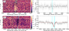 |
Fig. 6 Residual maps and transmission spectra around Hα (top panels) and He I NIR (bottom panels) lines. Left panels: residual maps in the stellar rest frame. The time since mid-transit time (Tc) is shown on the vertical axis, wavelength is on the horizontal axis, and relative absorption is color-coded. Dashed white horizontal lines indicate the first and fourth contacts. Cyan lines show the theoretical trace of the planetary signals. Right panels: transmission spectra obtained combining all the spectra, uncontaminated from stellar activity, between the first and fourth contacts. We show the original data in light gray and the data binned by 0.2 Å in black. The best Gaussian fit model is shown in red along with its lσ uncertainties (shaded red region). Dotted cyan vertical lines indicate the Hα (top) and the He I triplet (bottom) lines positions. All wavelengths in this figure are given in vacuum. |
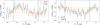 |
Fig. 7 Transit light curves of Hα (left) and He I triplet (right). The He I light curve has been constructed integrating the counts of the residual map in the planet rest frame around λ0 using σ (blue) and FWHM (orange) wavelength band passes from Table D.1. For the Hα light curve, we considered two generic band passes. The vertical lines represent the different contacts during the transit. Note the different y-axis scales between plots. |
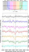 |
Fig. 8 Temporal evolution of the He I signal. Top panel: color scheme for the CARMENES spectra: pre-transit (black), ingress (blue), start (magenta), center (red), end (orange), egress (green), and post-transit (cyan). Horizontal bars represent the 5 min duration of the exposures. The transit model for HD 235088 b from Juliet (black solid line) is superimposed. Bottom panel: transmission spectra (TS) around the He I triplet line for the transit phases from top to bottom (consecutively offset by 2%). We show each TS binned by 0.2 Å with its uncertainties. Dashed black horizontal lines indicate the 0% level in each case, and dotted grey vertical line indicate the He I triplet line position. The wavelengths in this figure are given in vacuum. |
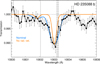 |
Fig. 9 Transmission spectrum of the He I triplet during transit. Measured absorption (solid dots) and estimated errors are shown in black (light gray data in the bottom/right panel of Fig. 6, but binned to half the number of the points and the error reduced by |

6 Modeling the He I absorption
We analyzed the He I absorption spectrum following the method used in previous studies for HD 209458 b, HD 189733 b, and GJ 3470 b (Lampón et al. 2020, Lampón et al. 2021b,a), and (more recently) for HAT-P-32b, WASP-69 b, GJ 1214 b, and WASP-76b (Lampón et al. 2023). Briefly, we used a one-dimensional hydrodynamic and spherically symmetric model, together with a non-local thermodynamic equilibrium model to calculate the He(23S) density distribution in the upper atmosphere of the planet (Lampón et al. 2020). The He(23S) absorption was subsequently computed by using a radiative transfer code for the primary transit geometry (Lampón et al. 2020), which includes Doppler line shapes broadened by the atmospheric temperature, by turbulent velocities and by the velocity of the outflowing gas along the line of sight. We computed the phase averaged synthetic absorption (i.e. the average from T1 to T4 contacts) and included the effects of the impact parameter. Some improvements and updates of the model are described in Lampón et al. (2023). Our estimate of the planetary mass corresponds to a planet-to-star mass ratio of 2.5 ×10⁻⁵. Using the formula given by Eggleton (1983), we estimate a Roche lobe radius of 2.2 RJ for the planet, which yields a transit depth of about 8.0% for the Roche volume. The observed 0.90% signal can, therefore, be plausibly caused by material within the planetary Roche lobe. In our detailed analysis (see below), we found that for an intermediate temperature of the best fits (see Fig. 10), the contribution of the layers inside the Roche lobe (under the assumption of no stellar winds, SWs) to the total absorption is about 80%. This contribution is larger for lower temperatures and smaller for higher temperatures. Also, it is larger if stellar winds are considered.
The model inputs specific to this planet are described below. The stellar and planet parameters of the system are listed in Table 1. A key input is the stellar flux from XUV to near-UV, covering the range from 1Å up to 2600 Å. The 1–1600 Å spectral energy distribution was modeled as described in Sect. 2.2, and the coverage up to 2600 Å was comleted by using the photo-spheric models by Castelli & Kurucz (2003). The H/He ratio is another key parameter affecting the mass-loss rate, Ṁ, and temperature ranges of the upper planetary atmosphere. In previous studies, this ratio has been constrained by using atomic hydrogen absorption measurements (Lyα or Hα; Lampón et al. 2020, 2021b, 2023) or by using theoretical arguments about the upper limit of the heating efficiency (Lampón et al. 2023). For most of the studied planets, a large H/He ratio, larger than 97/3, has been found. In particular, for the sub-Neptune GJ 1214 b, we derived a value of 98/2 (Lampón et al. 2023). This planet is, among those analyzed, the one closest in size to HD 235088 b; hence, given the lack of further information on the H/He ratio, we use the same value in this analysis.
We found that the He(23S) distribution of this planet is very extended, much more than in previously studied planets, including the sub-Neptune GJ 1214 b. An example of the modelled transmission for the combined transit (the average over the different phases) is shown in Fig. 9 for a thermospheric temperature of 3000 K and a sub-stellar mass-loss rate of 2.4 × 10¹⁰ g s−1. Because of the weak surface gravity of this planet, the velocities of the outflowing gas resulting from the hydrodynamic model are very large even at low radii, for instance, in the range of 5−15 km s−1 for r = 2−15 RP, thus inducing a very prominent broadening (compare blue and orange curves in Fig. 9). As described in Sect. 5.3, the absorption peak is shifted to blue wavelengths by −6.6 km s−1, suggesting that a large fraction of the observed atmosphere is flowing towards the observer. Similar blue shifts have been found for most of the planets with He(23S) detections. Since our 1D spherical and homogeneous model cannot predict it, we imposed a net shift of −6.6 km s−1 in our calculations.
With the method described above we constrain the mass-loss rate and temperature of the planet’s upper atmosphere to the ranges of (1.5−5) × 1010 g s−1 and T = 2750−3500 K (see Fig. 10). As this planet has a very extended atmosphere, the He(23S) absorption at high altitudes is significant and, hence, it is advisable to estimate the potential effects of the stellar wind (see e.g. Vidotto & Cleary 2020; Lampón et al. 2023). We did this by assuming that the atmosphere is still spherical but extended only up to the ionopause in the substellar direction (see more details in Lampón et al. 2023). The results (displayed as the black triangles in Fig. 10) show that a strong SW does not significantly change our nominal Ṁ-T ranges. Furthermore, as we could not constrain the H/He ratio, we also explored the effects of varying this ratio (see Fig. 10). The results show that increasing the H/He ratio to 99/1 does not significantly change the mass-loss rate. However, if the ratio were as low as 90/10 (unlikely given the previous results), then the mass-loss rate would be significantly lower.
Zhang et al. (2023) estimated a temperature of 6700 ± 300 K and a mass-loss rate of ~1.3 × 10¹¹ g s−1 for this planet. We derive significantly smaller values for both. Although we assumed different FXUV stellar fluxes (by a factor of three; see above), we found that this does not explain the differences. Instead, if we assume an upper boundary at 10−15 RP in our model and an H/He = 90/10 value (Zhang et al. 2023 used 11 RP and H/He = 90/10; M. Zhang 2023, priv. comm.) our results agree well. Nevertheless, as we would need an extraordinarily strong SW for confining the planetary wind at those altitudes, while current findings suggest a high H/He ratio, we think that this scenario is less likely and that the mass-loss rates and temperatures we derive are more plausible.
From a theoretical point of view, it is important to determine the hydrodynamic escape regime of the planets. Following the method used in previous studies (Lampón et al. 2021a, 2023), we found that for the assumed H/He ratio of 98/2, this planet is in the photon-limited regime, with a heating efficiency of 0.23 ± 0.03. However, for an H/He ratio of 90/10, although still in the photon-limited regime it approaches the energy-limited case, particularly at lower temperatures (3000 K).
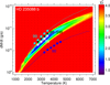 |
Fig. 10 Contour maps of the reduced χ2 of the He(23S) absorption obtained in the modeling for an H/He of 98/2. Dotted curves represent the best fits, with filled symbols denoting the constrained ranges for Ṁ and temperature for a confidence level of 95%. We over-plotted the curves and symbols when including the estimated effects of the stellar winds (H/He = 98/2, downward triangles) and for H/He ratios of 99/1 and 90/10. The labels correspond to the hydrogen percentage, e.g. ‘98’ for an H/He of 98/2. The small black dots represent the T-Ṁ grid of the simulations. |
7 Conclusions
We derived new stellar parameters for the K-type star HD 235088 and we obtained a new age estimation of 600–800 Myr. Furthermore, by using multiband photometry from MuSCAT2, we confirmed the planetary nature of HD 235088 b and refined its planetary parameters. With a radius of Rp = 2.045 ± 0.075 R⊕, HD 235088 b is a young sub-Neptune planet close to the “radius gap” valley (Fulton et al. 2017; Fulton & Petigura 2018). More interesting is the confirmation with CARMENES spectra of an evaporating He I atmosphere. Our excess absorption of −0.91 ± 0.11% is ~2σ deeper than the previous detection with Keck/NIRSPEC by Zhang et al. (2023). The difference in the absorption depths suggests possible He I variability, which should be clarified by further He I observations.
We also analyzed the He I signal detected in the transmission spectrum via hydrodynamical modeling. In comparison with previously studied planets (Lampón et al. 2023), the mass-loss rate and temperature of HD 235088 b are generally in the expected ranges. It has a low mass-loss rate corresponding to its moderate XUV irradiation level, and a low temperature as expected given its low gravitational potential. Its mass-loss rate and temperature are slightly lower than those of the sub-Neptunes GJ 3470 b and GJ 1214 b.
There are only three exoplanets smaller than HD 235088 b with atmospheric detections6, and all are only tentative and are based on Hubble Space Telescope or James Webb Space Telescope observations: GJ 1132 b (1.16 ± 0.11 R⊕, Swain et al. 2021), GJ486 b (1.34 ± 0.06R⊕, Moran et al. 2023), and LHS 1140 b (1.727 ± 0.032 R⊕, Edwards et al. 2021). In this work, we confirmed the presence of He I in the atmosphere of HD 235088 b, making this planet the smallest one with such a robust atmospheric detection – not only of He I but of any atom or molecule.
Acknowledgements
CARMENES is an instrument at the Centro Astronómico Hispano en Andalucía (CAHA) at Calar Alto (Almería, Spain), operated jointly by the Junta de Andalucía and the Instituto de Astrofísica de Andalucía (CSIC). CARMENES was funded by the Max-Planck-Gesellschaft (MPG), the Consejo Superior de Investigaciones Científicas (CSIC), the Ministerio de Economía y Competitividad (MINECO) and the European Regional Development Fund (ERDF) through projects FICTS-2011-02, ICTS-2017-07-CAHA-4, and CAHA16-CE-3978, and the members of the CARMENES Consortium (Max-Planck-Institut für Astronomie, Instituto de Astrofísica de Andalucía, Landessternwarte Königstuhl, Institut de Ciències de l’Espai, Institut für Astrophysik Göttingen, Universidad Complutense de Madrid, Thüringer Landessternwarte Tautenburg, Instituto de Astrofísica de Canarias, Hamburger Sternwarte, Centro de Astrobiología and Centro Astronómico Hispano-Alemán), with additional contributions by the MINECO, the Deutsche Forschungsgemeinschaft (DFG) through the Major Research Instrumentation Programme and Research Unit FOR2544 “Blue Planets around Red Stars”, the Klaus Tschira Stiftung, the states of Baden-Württemberg and Niedersachsen, and by the Junta de Andalucía. We acknowledge financial support from the State Agency for Research of the Spanish MCIU (AEI) through projects PID2019-110689RB-I00, PID2019-109522GB-C51,PID2019-109522GB-C5[4]/AEI/10.13039/501100011033, and the Centre of Excellence “Severo Ochoa” award to the Instituto de Astrofísica de Andalucía (CEX2021-001131-S). The first author acknowledges the special support from Padrina Conxa, Padrina Mercè, Jeroni, and Mercè. This work has made use of resources from AstroVallAlbaida-Mallorca collaboration. J.O.M. gratefully acknowledges the inspiring discussions with Maite Mateu, Alejandro Almodóvar, and Guillem Llodrà, and the warm support from Yess. This work is partly supported by JSPS KAKENHI Grant Numbers P17H04574, JP18H05439, JP21K13955, and JST CREST Grant Number JPMJCR1761. This paper is based on observations made with the MuSCAT2 instrument, developed by ABC, at Telescopio Carlos Sánchez operated on the island of Tenerife by the IAC in the Spanish Observatorio del Teide. This research was supported by the Excellence Cluster ORIGINS which is funded by the Deutsche Forschungsgemeinschaft (DFG, German Research Foundation) under Germany’s Excellence Strategy – EXC-2094 – 390783311. SC acknowledges support from DFG through project CZ 222/5-1.
Appendix A Testing the MUV flux level
One possibility for testing the actual level of the MUV flux would be the use of the UV filters onboard XMM-Newton, as suggested by Zhang et al. (2023) and references therein. The XMM-Newton pipeline reports a flux calibrated assuming a flat SED in the whole spectral range of the filter (AB flux). For sources with a steep SED in the UV region, as in the case of late-type stars, this is not a valid approach. Instead, the effective area combined of the XMM-Newton Optical Monitor (OM) filter must be convolved with the stellar SED. A similar procedure was followed by Zhang et al. (2023). The XMM-Newton pipeline provides, for the source at HD 235088 position, a count rate of 1.6 cts/s in the UVW2 (λλ 2120 ± 500 Å) filter, and 2.7cts/s in the UVM2 filter (λλ 2310 ± 480 Å). Although the effective area of these filters is mainly within the nominal limits, there is a non-negligible tail towards longer wavelengths.
To test the wavelengths at which the photons recorded in the OM/UVW2 filter had originated in, we extended our modelled SED up to 7000 Å, assuming a black-body emission for a star with temperature and size values as listed in Table 1. We applied a 30% reduction of the efficiency of the instrument due to degradation of the CCD7 over time. If we limit our test to the nominal UVW2 band-pass, we obtain 0.14 cts/s, just a ~9% of the observed count rate, but the use of the SED in the whole 1600–7000 Å spectral range result in a count rate of 1.59 cts/s. Same procedure with the OM/UVM2 filter yields 2.7 cts/s. Both values are in excellent agreement with the observed count rate. This implies that no correction is needed to the general level of our SED.
Figure A.1 shows the weighted count rate after convolving the effective area of the OM/UVW2 filter and an assumed SED. We used a flat SED (useful for AB magnitude or flux) in the nominal band-pass, and a realistic stellar SED in the whole spectral range. Although both combinations result in the same accumulated count rate, they yield quite different fluxes given the different distribution of photons along the spectrum. We find that 90% of the photons are actually coming from a wavelength range outside the nominal band-pass. This test indicates that the use of these filters to evaluate the stellar flux in the UV band must be taken with care.
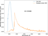 |
Fig. A.1 XMM-Newton OM/UVW2 weighted count rate along the actual bandpass of the filter. The effective area is convolved with a flat SED emission (only in nominal band-pass) and with a realistic stellar emission (modelled as a black-body emission, at the effective temperature of the star, at λ > 2700 Å). Most of the photons come from wavelengths outside the nominal band-pass (λλ 2120 ± 500 Å). |
Appendix B Photometrie fit extra figures
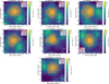 |
Fig. B.1 TESS target pixel file image of HD 235088 (TIC 293954617) observed in Sectors 14, 15, 16, 41, 54, 55, and 56 (made with tpfplotter). The pixels highlighted in red show the aperture used by TESS to get the photometry. The electron counts are color-coded. The position and sizes of the red circles represent the position and TESS magnitudes of nearby stars respectively. HD 235088 is marked with a ’×’ and labeled as #1. |
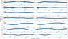 |
Fig. B.2 HD 235088 two-min cadence SAP TESS photometry from Sectors 14, 15, 16, 41, 54, 55, and 56 along with the transit plus GP model. Upward-pointing green triangles mark HD 235088 b’s transits. Upward-pointing red triangle marks the transit observed with CARMENES, and analyzed in this work. |
Appendix C Multi-color validation
 |
Fig. C.1 MuSCAT2 unfolded light-curves on each filter g, r, i and zs for the HD 235088 b. We have plotted 1σ uncertainties for the transit on each passband. |
Prior and posterior distributions from the eemce algorithm for the HD 235088 b.
Appendix D Additional figures and tables
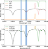 |
Fig. D.1 Telluric contamination close to the He I triplet lines. Upper panel: Simulation of the contamination of the spectrum of HD 235088 by H2O absorption and OH emission during the night of 6 August 2022. The green curve is a synthetic model of H2O absorption, the orange curve is a synthetic model of OH emission, and the black curve is the average of the normalised HD 235088 spectra. The dashed red line is the combination of synthetic telluric models and the HD 235088 spectrum. Lower panel: Averaged normalised HD 235088 spectra from 6 August 2022 CARMENES observations. Original spectrum is plotted in green, spectrum after molecfit correction is over-plotted in orange, and spectrum after molecfit and OH correction is over-plotted in black. The vertical blue dotted lines indicate the positions of the He I triplet lines, and the blue shaded region represents the planet trace in the stellar rest frame at vacuum wavelength. |
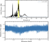 |
Fig. D.2 GLS periodogram of the TESS photometry that includes the combination of all sectors (top panel). The yellow vertical band shows the maximum peak found, whose period we associate with the rotation period of the star. Phase-folded plot for the period of 11.8 days (bottom panel). |
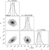 |
Fig. D.3 Corner plot for the nested sampling posterior distribution of the HD 235088 b He I signal. |
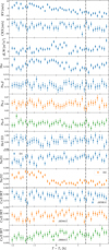 |
Fig. D.4 Time evolution of the serval products: RVs from VIS, activity indicators, and line indices; and the light curves of the H Paschen ß (Pa-ß 12821.6 Å; fifth panel), H Paschen γ (Paγ, 10941.1 Å; sixth panel), and H Paschen δ (Pa-δ, 10052.1 Å; seventh panel) lines, and the He ID3 line at 5877.2 Å (eighth panel). Vertical dash dotted black lines indicate the first and fourth contacts. |
References
- Alonso-Floriano, F. J., Snellen, I. A. G., Czesla, S., et al. 2019, A&A, 629, A110 [NASA ADS] [CrossRef] [EDP Sciences] [Google Scholar]
- Baruteau, C., Bai, X., Mordasini, C., & Mollière, P. 2016, Space Sci. Rev., 205, 77 [CrossRef] [Google Scholar]
- Bayo, A., Rodrigo, C., Barrado Y Navascués, D., et al. 2008, A&A, 492, 277 [NASA ADS] [CrossRef] [EDP Sciences] [Google Scholar]
- Benatti, S., Damasso, M., Borsa, F., et al. 2021, A&A, 650, A66 [NASA ADS] [CrossRef] [EDP Sciences] [Google Scholar]
- Bochanski, J. J., Faherty, J. K., Gagné, J., et al. 2018, AJ, 155, 149 [NASA ADS] [CrossRef] [Google Scholar]
- Borucki, W. J., Koch, D., Basri, G., et al. 2010, Science, 327, 977 [Google Scholar]
- Bouvier, J., Barrado, D., Moraux, E., et al. 2018, A&A, 613, A63 [NASA ADS] [CrossRef] [EDP Sciences] [Google Scholar]
- Brandt, T. D., & Huang, C. X. 2015, ApJ, 807, 24 [NASA ADS] [CrossRef] [Google Scholar]
- Brewer, J. M., Fischer, D. A., Valenti, J. A., & Piskunov, N. 2016, ApJS, 225, 32 [Google Scholar]
- Buchner, J., Georgakakis, A., Nandra, K., et al. 2014, A&A, 564, A125 [NASA ADS] [CrossRef] [EDP Sciences] [Google Scholar]
- Burrows, A. S., Heng, K., & Nampaisarn, T. 2011, ApJ, 736, 47 [NASA ADS] [CrossRef] [Google Scholar]
- Caballero, J. A., Guàrdia, J., López del Fresno, M., et al. 2016, SPIE Conf. Ser., 9910, 99100E [Google Scholar]
- Cannon, A. J., & Pickering, E. C. 1993, VizieR Online Data Catalog: III/135A [Google Scholar]
- Casasayas-Barris, N., Palle, E., Nowak, G., et al. 2017, A&A, 608, A135 [NASA ADS] [CrossRef] [EDP Sciences] [Google Scholar]
- Casasayas-Barris, N., Orell-Miquel, J., Stangret, M., et al. 2021, A&A, 654, A163 [NASA ADS] [CrossRef] [EDP Sciences] [Google Scholar]
- Castelli, F., & Kurucz, R. L. 2003, IAU Symp., 210, A20 [Google Scholar]
- Cummings, J. D., Deliyannis, C. P., Maderak, R. M., & Steinhauer, A. 2017, AJ, 153, 128 [Google Scholar]
- Curtis, J. L., Agüeros, M. A., Douglas, S. T., & Meibom, S. 2019, ApJ, 879, 49 [Google Scholar]
- Cushing, M. C., Rayner, J. T., & Vacca, W. D. 2005, ApJ, 623, 1115 [Google Scholar]
- Cutri, R. M., Skrutskie, M. F., van Dyk, S., et al. 2003, VizieR Online Data Catalog: II/246 [Google Scholar]
- Czesla, S., Lampón, M., Sanz-Forcada, J., et al. 2022, A&A, 657, A6 [NASA ADS] [CrossRef] [EDP Sciences] [Google Scholar]
- David, T. J., Hillenbrand, L. A., Petigura, E. A., et al. 2016, Nature, 534, 658 [CrossRef] [Google Scholar]
- David, T. J., Petigura, E. A., Luger, R., et al. 2019, ApJ, 885, L12 [Google Scholar]
- Dawson, R. I., & Johnson, J. A. 2018, ARA&A, 56, 175 [Google Scholar]
- Douglas, S. T., Agüeros, M. A., Covey, K. R., & Kraus, A. 2017, ApJ, 842, 83 [Google Scholar]
- Douglas, S. T., Curtis, J. L., Agüeros, M. A., et al. 2019, ApJ, 879, 100 [Google Scholar]
- Ducati, J. R. 2002, VizieR Online Data Catalog: II/237 [Google Scholar]
- Edwards, B., Changeat, Q., Mori, M., et al. 2021, AJ, 161, 44 [Google Scholar]
- Eggleton, P. P. 1983, ApJ, 268, 368 [Google Scholar]
- Esparza-Borges, E., Parviainen, H., Murgas, F., et al. 2022, A&A, 666, A10 [NASA ADS] [CrossRef] [EDP Sciences] [Google Scholar]
- Espinoza, N. 2018, RNAAS, 2, 209 [Google Scholar]
- Espinoza, N., Kossakowski, D., & Brahm, R. 2019, MNRAS, 490, 2262 [Google Scholar]
- Fernandes, J., Gafeira, R., & Andersen, J. 2021, A&A, 647, A90 [NASA ADS] [CrossRef] [EDP Sciences] [Google Scholar]
- Feroz, F., Hobson, M. P., & Bridges, M. 2009, MNRAS, 398, 1601 [NASA ADS] [CrossRef] [Google Scholar]
- Foreman-Mackey, D., Agol, E., Angus, R., & Ambikasaran, S. 2017, AJ, 154, 220 [NASA ADS] [CrossRef] [Google Scholar]
- Foster, A. R., Ji, L., Smith, R. K., & Brickhouse, N. S. 2012, ApJ, 756, 128 [Google Scholar]
- Fuhrmeister, B., Czesla, S., Hildebrandt, L., et al. 2020, A&A, 640, A52 [NASA ADS] [CrossRef] [EDP Sciences] [Google Scholar]
- Fulton, B. J., & Petigura, E. A. 2018, AJ, 156, 264 [Google Scholar]
- Fulton, B. J., Petigura, E. A., Howard, A. W., et al. 2017, AJ, 154, 109 [Google Scholar]
- Gaia Collaboration 2020, VizieR Online Data Catalog: I/350 [Google Scholar]
- Gaia Collaboration (Klioner, S. A., et al..) 2022, A&A, 667, A148 [NASA ADS] [CrossRef] [EDP Sciences] [Google Scholar]
- Gaidos, E., Hirano, T., Lee, R. A., et al. 2023, MNRAS, 518, 3777 [Google Scholar]
- Guerrero, N. M., Seager, S., Huang, C. X., et al. 2021, ApJS, 254, 39 [NASA ADS] [CrossRef] [Google Scholar]
- Gustafsson, B., Edvardsson, B., Eriksson, K., et al. 2008, A&A, 486, 951 [NASA ADS] [CrossRef] [EDP Sciences] [Google Scholar]
- Heiter, U., Lind, K., Bergemann, M., et al. 2021, A&A, 645, A106 [EDP Sciences] [Google Scholar]
- Høg, E., Fabricius, C., Makarov, V. V., et al. 2000, A&A, 355, L27 [Google Scholar]
- Houck, J. C., & Denicola, L. A. 2000, ASP Conf. Ser., 216, 591 [Google Scholar]
- Howell, S. B., Sobeck, C., Haas, M., et al. 2014, PASP, 126, 398 [Google Scholar]
- Johnson, H. L., & Morgan, W. W. 1953, ApJ, 117, 313 [NASA ADS] [CrossRef] [Google Scholar]
- Johnson, D. R. H., & Soderblom, D. R. 1987, AJ, 93, 864 [Google Scholar]
- Kausch, W., Noll, S., Smette, A., et al. 2015, A&A, 576, A78 [NASA ADS] [CrossRef] [EDP Sciences] [Google Scholar]
- Kipping, D. M. 2013, MNRAS, 435, 2152 [Google Scholar]
- Kirk, J., Alam, M. K., López-Morales, M., & Zeng, L. 2020, AJ, 159, 115 [Google Scholar]
- Kreidberg, L. 2015, PASP, 127, 1161 [Google Scholar]
- Lampón, M., López-Puertas, M., Lara, L. M., et al. 2020, A&A, 636, A13 [NASA ADS] [CrossRef] [EDP Sciences] [Google Scholar]
- Lampón, M., López-Puertas, M., Czesla, S., et al. 2021a, A&A, 648, L7 [CrossRef] [EDP Sciences] [Google Scholar]
- Lampón, M., López-Puertas, M., Sanz-Forcada, J., et al. 2021b, A&A, 647, A129 [EDP Sciences] [Google Scholar]
- Lampón, M., López-Puertas, M., Sanz-Forcada, J., et al. 2023, A&A, 673, A140 [NASA ADS] [CrossRef] [EDP Sciences] [Google Scholar]
- Lodieu, N., Rebolo, R., & Pérez-Garrido, A. 2018, A&A, 615, L12 [NASA ADS] [CrossRef] [EDP Sciences] [Google Scholar]
- Maldonado, J., Colombo, S., Petralia, A., et al. 2022, A&A, 663, A142 [NASA ADS] [CrossRef] [EDP Sciences] [Google Scholar]
- Mamajek, E. E., & Hillenbrand, L. A. 2008, ApJ, 687, 1264 [Google Scholar]
- Marfil, E., Tabernero, H. M., Montes, D., et al. 2020, MNRAS, 492, 5470 [NASA ADS] [CrossRef] [Google Scholar]
- Matsuhara, H., Wada, T., Matsuura, S., et al. 2006, PASJ, 58, 673 [NASA ADS] [Google Scholar]
- Montes, D., López-Santiago, J., Gálvez, M. C., et al. 2001, MNRAS, 328, 45 [NASA ADS] [CrossRef] [Google Scholar]
- Moran, S. E., Stevenson, K. B., Sing, D. K., et al. 2023, ApJ, 948, L11 [NASA ADS] [CrossRef] [Google Scholar]
- Morello, G., Parviainen, H., Murgas, F., et al. 2023, A&A, 673, A32 [NASA ADS] [CrossRef] [EDP Sciences] [Google Scholar]
- Morris, R. L., Twicken, J. D., Smith, J. C., et al. 2017, Kepler Science DocumentKSCI-19081-002, 6 [Google Scholar]
- Murgas, F., Nowak, G., Masseron, T., et al. 2022, A&A, 668, A158 [NASA ADS] [CrossRef] [EDP Sciences] [Google Scholar]
- Narita, N., Fukui, A., Kusakabe, N., et al. 2019, J. Astron. Teles. Instrum. Syst., 5, 015001 [Google Scholar]
- Nordström, B., Mayor, M., Andersen, J., et al. 2004, A&A, 418, 989 [Google Scholar]
- Nortmann, L., Pallé, E., Salz, M., et al. 2018, Science, 362, 1388 [Google Scholar]
- Noyes, R. W., Hartmann, L. W., Baliunas, S. L., Duncan, D. K., & Vaughan, A. H. 1984, ApJ, 279, 763 [Google Scholar]
- Orell-Miquel, J., Murgas, F., Pallé, E., et al. 2022, A&A, 659, A55 [NASA ADS] [CrossRef] [EDP Sciences] [Google Scholar]
- Owen, J. E., & Lai, D. 2018, MNRAS, 479, 5012 [Google Scholar]
- Owen, J. E., & Wu, Y. 2017, ApJ, 847, 29 [Google Scholar]
- Palle, E., Nortmann, L., Casasayas-Barris, N., et al. 2020a, A&A, 638, A61 [EDP Sciences] [Google Scholar]
- Palle, E., Oshagh, M., Casasayas-Barris, N., et al. 2020b, A&A, 643, A25 [EDP Sciences] [Google Scholar]
- Parviainen, H. 2015, MNRAS, 450, 3233 [Google Scholar]
- Parviainen, H., Tingley, B., Deeg, H. J., et al. 2019, A&A, 630, A89 [NASA ADS] [CrossRef] [EDP Sciences] [Google Scholar]
- Parviainen, H., Palle, E., Zapatero-Osorio, M. R., et al. 2020, A&A, 633, A28 [NASA ADS] [CrossRef] [EDP Sciences] [Google Scholar]
- Parviainen, H., Palle, E., Zapatero-Osorio, M. R., et al. 2021, A&A, 645, A16 [NASA ADS] [CrossRef] [EDP Sciences] [Google Scholar]
- Plavchan, P., Barclay, T., Gagné, J., et al. 2020, Nature, 582, 497 [Google Scholar]
- Plez, B. 2012, Astrophysics Source Code Library [record ascl:1205.004] [Google Scholar]
- Quirrenbach, A., Amado, P. J., Caballero, J. A., et al. 2014, SPIE Conf. Ser., 9147, 91471F [Google Scholar]
- Quirrenbach, A., CARMENES Consortium, Amado, P. J., et al. 2020, SPIE Conf. Ser., 11447, 114473C [Google Scholar]
- Rebull, L. M., Stauffer, J. R., Bouvier, J., et al. 2016, AJ, 152, 113 [Google Scholar]
- Ricker, G. R., Winn, J. N., Vanderspek, R., et al. 2015, J. Astron. Teles. Instrum. Syst., 1, 014003 [Google Scholar]
- Salz, M., Czesla, S., Schneider, P. C., et al. 2018, A&A, 620, A97 [NASA ADS] [CrossRef] [EDP Sciences] [Google Scholar]
- Sanz-Forcada, J., Micela, G., Ribas, I., et al. 2011, A&A, 532, A6 [NASA ADS] [CrossRef] [EDP Sciences] [Google Scholar]
- Schlaufman, K. C. 2010, ApJ, 719, 602 [NASA ADS] [CrossRef] [Google Scholar]
- Skrutskie, M. F., Cutri, R. M., Stiening, R., et al. 2006, AJ, 131, 1163 [NASA ADS] [CrossRef] [Google Scholar]
- Smette, A., Sana, H., Noll, S., et al. 2015, A&A, 576, A77 [NASA ADS] [CrossRef] [EDP Sciences] [Google Scholar]
- Soubiran, C., Jasniewicz, G., Chemin, L., et al. 2018, A&A, 616, A7 [NASA ADS] [CrossRef] [EDP Sciences] [Google Scholar]
- Spake, J. J., Oklopčić, A., & Hillenbrand, L. A. 2021, AJ, 162, 284 [NASA ADS] [CrossRef] [Google Scholar]
- Speagle, J. S. 2020, MNRAS, 493, 3132 [Google Scholar]
- Stassun, K. G., Oelkers, R. J., Pepper, J., et al. 2018, AJ, 156, 102 [Google Scholar]
- Swain, M. R., Estrela, R., Roudier, G. M., et al. 2021, AJ, 161, 213 [NASA ADS] [CrossRef] [Google Scholar]
- Tabernero, H. M., Marfil, E., Montes, D., & González Hernández, J. I. 2022, A&A, 657, A66 [NASA ADS] [CrossRef] [EDP Sciences] [Google Scholar]
- Tinetti, G., Drossart, P., Eccleston, P., et al. 2018, Exp. Astron., 46, 135 [NASA ADS] [CrossRef] [Google Scholar]
- van Leeuwen, F. 2007, A&A, 474, 653 [CrossRef] [EDP Sciences] [Google Scholar]
- Vidotto, A. A., & Cleary, A. 2020, MNRAS, 494, 2417 [Google Scholar]
- Wright, E. L., Eisenhardt, P. R. M., Mainzer, A. K., et al. 2010, AJ, 140, 1868 [Google Scholar]
- Wright, N. J., Drake, J. J., Mamajek, E. E., & Henry, G. W. 2011, ApJ, 743, 48 [Google Scholar]
- Wyttenbach, A., Ehrenreich, D., Lovis, C., Udry, S., & Pepe, F. 2015, A&A, 577, A62 [NASA ADS] [CrossRef] [EDP Sciences] [Google Scholar]
- York, D. G., Adelman, J., Anderson, John E., J., et al. 2000, AJ, 120, 1579 [NASA ADS] [CrossRef] [Google Scholar]
- Zechmeister, M., & Kürster, M. 2009, A&A, 496, 577 [CrossRef] [EDP Sciences] [Google Scholar]
- Zechmeister, M., Anglada-Escudé, G., & Reiners, A. 2014, A&A, 561, A59 [NASA ADS] [CrossRef] [EDP Sciences] [Google Scholar]
- Zechmeister, M., Reiners, A., Amado, P. J., et al. 2018, A&A, 609, A12 [NASA ADS] [CrossRef] [EDP Sciences] [Google Scholar]
- Zhang, M., Knutson, H. A., Wang, L., Dai, F., & Barragán, O. 2022a, AJ, 163, 67 [NASA ADS] [CrossRef] [Google Scholar]
- Zhang, M., Knutson, H. A., Wang, L., et al. 2022b, AJ, 163, 68 [NASA ADS] [CrossRef] [Google Scholar]
- Zhang, M., Knutson, H. A., Dai, F., et al. 2023, AJ, 165, 62 [NASA ADS] [CrossRef] [Google Scholar]
According to the ExoAtmospheres database (http://research.iac.es/proyecto/exoatmospheres/index.php).
All Tables
Prior and posterior distributions from the eemce algorithm for the HD 235088 b.
All Figures
|
Fig. 1 Photometric spectral energy distribution of HD 235088 (circles) from 0.3 through ~25 µm. A black-body source with a temperature of 5050 K (solid line) is added for the sole purpose of demonstrating that all fluxes are photospheric in origin and there are no infrared flux excesses at long wavelengths. Vertical error bars denote flux uncertainties and horizontal error bars account for the width of the photometric passbands. |
| In the text | |
|
Fig. 2 Rotation period distribution as a function of color G-J for the Pleiades (~125 Myr; Rebull et al. 2016), Praesepe (~590 Myr; Douglas et al. 2017), Hyades (~650 Myr; Douglas et al. 2019) and NGC 6811 (~1000 Myr; Curtis et al. 2019) clusters. The gold star represents HD 235088. |
| In the text | |
|
Fig. 3 Equivalent width distribution of Li I as a function of the effective temperature for the Pleiades (~125 Myr; Bouvier et al. 2018), Praesepe (~590 Myr), and Hyades (~650 Myr; Cummings et al. 2017). The gold triangle represents HD 235088. |
| In the text | |
|
Fig. 4 UVW velocity diagram for HD 235088 (gold star). The members of the Castor moving group, Hyades supercluster (Hs), IC 2391 supercluster, Local Association (LA), and Ursa Major group (UMa) from Montes et al. (2001) are included. The ellipses represent the 3σ values of the UVW for each Young Moving Group. HD 235088 agrees with the Hyades supercluster. |
| In the text | |
|
Fig. 5 HD 235088 TESS photometry (blue dots with error bars) phase-folded to the period, P, and central time of transit, t0, (shown above each panel, t0 units are BJD – 2 457 000) derived from the juliet fit. The black line is the best transit model for HD 235088 b. Orange points show binned photometry for visualization. The GP model was removed from the data. |
| In the text | |
|
Fig. 6 Residual maps and transmission spectra around Hα (top panels) and He I NIR (bottom panels) lines. Left panels: residual maps in the stellar rest frame. The time since mid-transit time (Tc) is shown on the vertical axis, wavelength is on the horizontal axis, and relative absorption is color-coded. Dashed white horizontal lines indicate the first and fourth contacts. Cyan lines show the theoretical trace of the planetary signals. Right panels: transmission spectra obtained combining all the spectra, uncontaminated from stellar activity, between the first and fourth contacts. We show the original data in light gray and the data binned by 0.2 Å in black. The best Gaussian fit model is shown in red along with its lσ uncertainties (shaded red region). Dotted cyan vertical lines indicate the Hα (top) and the He I triplet (bottom) lines positions. All wavelengths in this figure are given in vacuum. |
| In the text | |
|
Fig. 7 Transit light curves of Hα (left) and He I triplet (right). The He I light curve has been constructed integrating the counts of the residual map in the planet rest frame around λ0 using σ (blue) and FWHM (orange) wavelength band passes from Table D.1. For the Hα light curve, we considered two generic band passes. The vertical lines represent the different contacts during the transit. Note the different y-axis scales between plots. |
| In the text | |
|
Fig. 8 Temporal evolution of the He I signal. Top panel: color scheme for the CARMENES spectra: pre-transit (black), ingress (blue), start (magenta), center (red), end (orange), egress (green), and post-transit (cyan). Horizontal bars represent the 5 min duration of the exposures. The transit model for HD 235088 b from Juliet (black solid line) is superimposed. Bottom panel: transmission spectra (TS) around the He I triplet line for the transit phases from top to bottom (consecutively offset by 2%). We show each TS binned by 0.2 Å with its uncertainties. Dashed black horizontal lines indicate the 0% level in each case, and dotted grey vertical line indicate the He I triplet line position. The wavelengths in this figure are given in vacuum. |
| In the text | |
|
Fig. 9 Transmission spectrum of the He I triplet during transit. Measured absorption (solid dots) and estimated errors are shown in black (light gray data in the bottom/right panel of Fig. 6, but binned to half the number of the points and the error reduced by |
| In the text | |
|
Fig. 10 Contour maps of the reduced χ2 of the He(23S) absorption obtained in the modeling for an H/He of 98/2. Dotted curves represent the best fits, with filled symbols denoting the constrained ranges for Ṁ and temperature for a confidence level of 95%. We over-plotted the curves and symbols when including the estimated effects of the stellar winds (H/He = 98/2, downward triangles) and for H/He ratios of 99/1 and 90/10. The labels correspond to the hydrogen percentage, e.g. ‘98’ for an H/He of 98/2. The small black dots represent the T-Ṁ grid of the simulations. |
| In the text | |
|
Fig. A.1 XMM-Newton OM/UVW2 weighted count rate along the actual bandpass of the filter. The effective area is convolved with a flat SED emission (only in nominal band-pass) and with a realistic stellar emission (modelled as a black-body emission, at the effective temperature of the star, at λ > 2700 Å). Most of the photons come from wavelengths outside the nominal band-pass (λλ 2120 ± 500 Å). |
| In the text | |
|
Fig. B.1 TESS target pixel file image of HD 235088 (TIC 293954617) observed in Sectors 14, 15, 16, 41, 54, 55, and 56 (made with tpfplotter). The pixels highlighted in red show the aperture used by TESS to get the photometry. The electron counts are color-coded. The position and sizes of the red circles represent the position and TESS magnitudes of nearby stars respectively. HD 235088 is marked with a ’×’ and labeled as #1. |
| In the text | |
|
Fig. B.2 HD 235088 two-min cadence SAP TESS photometry from Sectors 14, 15, 16, 41, 54, 55, and 56 along with the transit plus GP model. Upward-pointing green triangles mark HD 235088 b’s transits. Upward-pointing red triangle marks the transit observed with CARMENES, and analyzed in this work. |
| In the text | |
|
Fig. C.1 MuSCAT2 unfolded light-curves on each filter g, r, i and zs for the HD 235088 b. We have plotted 1σ uncertainties for the transit on each passband. |
| In the text | |
|
Fig. D.1 Telluric contamination close to the He I triplet lines. Upper panel: Simulation of the contamination of the spectrum of HD 235088 by H2O absorption and OH emission during the night of 6 August 2022. The green curve is a synthetic model of H2O absorption, the orange curve is a synthetic model of OH emission, and the black curve is the average of the normalised HD 235088 spectra. The dashed red line is the combination of synthetic telluric models and the HD 235088 spectrum. Lower panel: Averaged normalised HD 235088 spectra from 6 August 2022 CARMENES observations. Original spectrum is plotted in green, spectrum after molecfit correction is over-plotted in orange, and spectrum after molecfit and OH correction is over-plotted in black. The vertical blue dotted lines indicate the positions of the He I triplet lines, and the blue shaded region represents the planet trace in the stellar rest frame at vacuum wavelength. |
| In the text | |
|
Fig. D.2 GLS periodogram of the TESS photometry that includes the combination of all sectors (top panel). The yellow vertical band shows the maximum peak found, whose period we associate with the rotation period of the star. Phase-folded plot for the period of 11.8 days (bottom panel). |
| In the text | |
|
Fig. D.3 Corner plot for the nested sampling posterior distribution of the HD 235088 b He I signal. |
| In the text | |
|
Fig. D.4 Time evolution of the serval products: RVs from VIS, activity indicators, and line indices; and the light curves of the H Paschen ß (Pa-ß 12821.6 Å; fifth panel), H Paschen γ (Paγ, 10941.1 Å; sixth panel), and H Paschen δ (Pa-δ, 10052.1 Å; seventh panel) lines, and the He ID3 line at 5877.2 Å (eighth panel). Vertical dash dotted black lines indicate the first and fourth contacts. |
| In the text | |
Current usage metrics show cumulative count of Article Views (full-text article views including HTML views, PDF and ePub downloads, according to the available data) and Abstracts Views on Vision4Press platform.
Data correspond to usage on the plateform after 2015. The current usage metrics is available 48-96 hours after online publication and is updated daily on week days.
Initial download of the metrics may take a while.