| Issue |
A&A
Volume 693, January 2025
|
|
|---|---|---|
| Article Number | A32 | |
| Number of page(s) | 26 | |
| Section | Planets, planetary systems, and small bodies | |
| DOI | https://doi.org/10.1051/0004-6361/202452236 | |
| Published online | 24 December 2024 | |
The GAPS Programme at TNG
LXV. Precise density measurement of TOI-1430 b, a young planet with an evaporating atmosphere
1
Dipartimento di Fisica e Astronomia “Galileo Galilei” – Università degli Studi di Padova,
Vicolo dell’Osservatorio 3,
35122
Padova,
Italy
2
INAF – Osservatorio Astronomico di Padova,
Vicolo dell’Osservatorio 5,
Padova
35122,
Italy
3
Centro di Ateneo di Studi e Attività Spaziali “G. Colombo” – Università degli Studi di Padova,
Via Venezia 15,
35131
Padova,
Italy
4
Department of Astronomy and Astrophysics, University of California,
Santa Cruz,
CA
95060,
USA
5
INAF – Osservatorio Astronomico di Palermo,
Piazza del Parlamento 1,
90134
Palermo (PA),
Italy
6
Dipartimento di Scienza e Alta Tecnologia, Università dell’Insubria,
Via Valleggio 11,
22100
Como,
Italy
7
ESO-European Southern Observatory,
Alonso de Cordova 3107,
Vitacura,
Santiago,
Chile
8
INAF – Osservatorio Astronomico di Roma,
Via Frascati 33,
00078
Monte Porzio Catone (Roma),
Italy
9
Dipartimento di Fisica, Università degli Studi di Roma Tor Vergata,
via della Ricerca Scientifica 1,
00133
Roma,
Italy
10
Department of Physics and Astronomy, The University of Texas,
Rio Grande Valley,
Brownsville,
TX
78520,
USA
11
Leibniz-Institut für Astrophysik Potsdam (AIP),
An der Sternwarte 16,
14482
Potsdam,
Germany
12
INAF – Osservatorio Astrofisico di Torino,
Via Osservatorio 20,
10025,
Pino Torinese,
Italy
13
INAF – Osservatorio Astronomico di Trieste,
via Tiepolo 11,
34143
Trieste,
Italy
14
INAF – Osservatorio Astronomico di Brera,
Via E. Bianchi 46,
23807
Merate (LC),
Italy
15
Center for Astrophysics | Harvard & Smithsonian,
60 Garden Street,
Cambridge,
MA
02138,
USA
16
Dipartimento di Fisica, Sapienza Università di Roma,
Piazzale Aldo Moro 5,
00185
Roma,
Italy
17
Fundación Galileo Galilei – INAF,
Rambla J.A. Fernandez P., 7,
38712 S.C.
Tenerife,
Spain
18
INAF – Osservatorio Astrofisico di Catania,
Via S. Sofia 78,
95123
Catania,
Italy
19
Max Planck Institute for Astronomy,
Königstuhl 17,
69117
Heidelberg,
Germany
20
South African Astronomical Observatory,
PO Box 9,
Observatory,
Cape Town
7935,
South Africa
21
Kotizarovci Observatory,
Sarsoni 90,
51216
Viskovo,
Croatia
★ Corresponding author; This email address is being protected from spambots. You need JavaScript enabled to view it.
Received:
13
September
2024
Accepted:
16
November
2024
Abstract
Context. Small-sized (<4 R⊕) exoplanets in tight orbits around young stars (10–1000 Myr) give us the opportunity to investigate the mechanisms that led to their formation, the evolution of their physical and orbital properties, and, in particular, their atmospheres. Thanks to the all-sky survey carried out by the TESS spacecraft, many of these exoplanets have been discovered, and have subsequently been characterized with dedicated follow-up observations.
Aims. In the context of a collaboration among the Global Architecture of Planetary Systems (GAPS) team, the TESS-Keck Survey (TKS) team, and the California Planet Search (CPS) team, we measured – with a high level of precision – the mass and the radius of TOI-1430 b, a young (~700 Myr) exoplanet with an escaping He atmosphere orbiting the K-dwarf star HD 235088 (TOI-1430).
Methods. By adopting appropriate stellar parameters, which were measured in this work, we were able to simultaneously model the signals due to strong stellar activity and the transiting planet TOI-1430 b in both photometric and spectroscopic series. This allowed us to measure both the radius and mass (and consequently the density) of the planet with high precision, and to reconstruct the evolution of its atmosphere.
Results. TOI-1430 is an active K-dwarf star born 700 ± 150 Myr ago, with a rotation period of Prot ~ 12 days. This star hosts a mini-Neptune, whose orbital period is Pb = 7.434133 ± 0.000004 days. Thanks to long-term photometric and spectroscopic monitoring of this target performed with TESS, HARPS-N, HIRES, and APF, we estimate a radius of RP,b = 1.98 ± 0.07 R⊕, a mass of MP,b = 4.2 ± 0.8 M⊕, and thus a planetary density of ρb = 0.5 ± 0.1 ρ⊕. TOI-1430 b is therefore a low-density mini-Neptune with an extended atmosphere, and is at the edge of the radius gap. Because this planet is known to have an evaporating atmosphere of He, we reconstructed its atmospheric history. Our analysis supports the scenario in which, shortly after its birth, TOI-1430 b was super-puffy, with a radius 5 × −13 × and a mass 1.5 × −2 × the values of today; in ~200 Myr from now, TOI-1430 b should lose its envelope, showing its Earth-size core. We also looked for signals from a second planet in the spectroscopic and photometric series, without detecting any.
Key words: techniques: radial velocities / planets and satellites: atmospheres / planets and satellites: fundamental parameters / planets and satellites: individual: TOI-1430b / stars: fundamental parameters / stars: individual: HD 235088
© The Authors 2024
 Open Access article, published by EDP Sciences, under the terms of the Creative Commons Attribution License (https://creativecommons.org/licenses/by/4.0), which permits unrestricted use, distribution, and reproduction in any medium, provided the original work is properly cited.
This article is published in open access under the Subscribe to Open model. This email address is being protected from spambots. You need JavaScript enabled to view it. to support open access publication.
1 Introduction
Young exoplanets (≲1 Gyr) offer a unique opportunity to understand the mechanisms of formation and evolution of planetary systems. The Transiting Exoplanet Survey Satellite (TESS; Ricker et al. 2015) has allowed us to increase the number of planets belonging to this scarcely populated category. Indeed, in the last five years, many projects have begun searching for young planets with TESS (e.g., Bouma et al. 2019; Nardiello et al. 2019; Newton et al. 2019; Battley et al. 2022). Despite difficulties related to the large variations of the light curves of active stars, many candidate exoplanets have been found both around members of young stellar clusters, associations, and moving groups (e.g., Bouma et al. 2020; Rizzuto et al. 2020; Newton et al. 2021; Mann et al. 2020; Nardiello 2020; Nardiello et al. 2021; Tofflemire et al. 2021; Mann et al. 2022; Wood et al. 2023; Thao et al. 2024) and orbiting young single stars (e.g., Giacalone et al. 2022a,b; Vach et al. 2022; Mantovan et al. 2022). Intensive spectroscopic follow-up studies of these objects have not only allowed constraints to be put on the planetary masses (e.g., Benatti et al. 2019, 2021; Barragán et al. 2022b; Kabáth et al. 2022; Desidera et al. 2023; Damasso et al. 2023; Barragán et al. 2024; Damasso et al. 2024; Mantovan et al. 2024a; Carleo et al. 2024) but have also led to the identification of their extended (escaping) atmospheres (e.g., Orell-Miquel et al. 2023; Zhang et al. 2023; Gaidos et al. 2023; Pérez-González et al. 2024; Masson et al. 2024). The discovery and the full characterization of young exoplanets help us constrain the timescales on which mechanisms like photo-evaporation (Owen & Wu 2013; Lopez & Fortney 2014) and core-powered mass loss (Ginzburg et al. 2018; Gupta & Schlichting 2019) act.
The aim of the Global Architecture of Planetary Systems (GAPS) collaboration (Covino et al. 2013) is to carry out spectroscopic follow-up studies of transiting and non-transiting exoplanets in order to determine planetary masses, measure orbital properties (Damasso et al. 2015), detect planetary atmospheres (e.g., Pino et al. 2022; Sicilia et al. 2024; Guilluy et al. 2024), and characterize the host stars (Maldonado et al. 2022; Biazzo et al. 2022; Claudi et al. 2024). In particular, the Young Objects program (Carleo et al. 2020) provides a spectroscopic followup of planets younger than 750–1000 Myr. Under this program, we carried out a three-year observational campaign of the young K-dwarf star HD 235088 (also called TOI-1430; V ~ 9.2), which hosts a potential transiting exoplanet (TOI-1430 b), as reported in Giacalone et al. (2021, false-positive probability equal to 0.03). Zhang et al. (2023) detected an atmosphere on this planet using Keck/NIRSPEC, as did Orell-Miquel et al. (2023) based on CARMENES data; both detected the presence of an evaporating helium atmosphere. Polanski et al. (2024) detected a hint (<2σ) of the TOI-1430 b signal using radial velocity (RV) measurements.
In this work, we detect and characterize TOI-1430 b, making use of a combination of photometric data from nine TESS sectors and spectroscopic data collected with the High Accuracy Radial velocity Planet Searcher for the Northern hemisphere (HARPS-N, Cosentino et al. 2012) on the Telescopio Nazionale Galileo (TNG) for the GAPS program and with the High Resolution Echelle Spectrometer (HIRES) on the 10 m Keck I telescope for the TESS-Keck Survey (Dalba et al. 2020) and California Planet Search programs. On the basis of our results, we characterize the evolutionary history of TOI-1430 b’s atmosphere.
2 Observations and data reduction
2.1 TESS data
The dataset of TOI-1430 used in this work has been collected by TESS in short-cadence mode in nine different sectors (see Fig. 1): during the second Cycle of TESS operations in Sectors 14, 15, and 16 (18 July 2019–7 October 2019), during Sector 41 (fourth Cycle of TESS mission, 23 July 2021–20 August 2021), in Sectors 54, 55, and 56 between cycle 4 and cycle 5 (1 September 2022–30 September 2022), and finally in cycle 6 during sectors 75 and 76 (30 January 2024–26 March 2024).
In this work, we did not make use of the Pre-search Data Conditioning Simple Aperture Photometry (PDCSAP) light curves (Smith et al. 2012; Stumpe et al. 2012, 2014) because of systematic effects introduced by the TESS official correction pipeline in the cases of variable stars (see Fig. A.1 in Nardiello et al. 2022 and Fig. A.1 of this work). Moreover, we found that the SAP light curves also suffer from a systematic effect introduced by contaminated local background (see panels b and c of Fig. A.1): in fact, we found a periodic signal (~2.81 days) due to a close-by eclipsing binary (TIC 293954660, Shi et al. 2022) that clearly affected the local background that is subtracted to the pixel values inside the photometric aperture adopted to extract the light curve of TOI-1430.
We extracted the light curves of TOI-1430 (and of all the stars within the same Camera/CCD) and we corrected them for systematic effects adopting the PATHOS pipeline presented by Nardiello et al. (2019) (for a detailed description of the pipeline, see also Nardiello et al. 2020; Nardiello 2020; Nardiello et al. 2021), based on the PSF-based approach developed by Nardiello et al. (2015, 2016b) and also used for Kepler/K2 data (see, e.g., Libralato et al. 2016; Nardiello et al. 2016a). During the extraction of stellar fluxes, for the calculation of the local background, we took care to exclude all the pixels contaminated by the flux of the neighbor stars by using masks obtained from the PSF models and the Gaia DR3 catalog.
For the analysis described in the next sections, we removed all the points flagged with the quality parameter DQUALITY>0. The analyzed light curve is shown in Fig. 2.
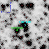 |
Fig. 1 Finding chart (15 × 15 arcmin2) of TOI-1430 (cyan diamond) from a TESS Full Frame Image. Neighboring stars with G ≤ 15 are identified with red circles, the radii of which are inversely proportional to the difference between the magnitude of TOI-1430 and that of its neighbors. The green circle indicates the eclipsing binary that generates the spurious signal in the SAP light curves. |
2.2 KELT
In this work, we used the light curves obtained during the Kilodegree Extremely Little Telescope (KELT) survey (Pepper et al. 2007). The photometric series contains 2847 points (see Fig. 2). Observations were carried out with KELT-North (Winer Observatory, Sonoita, Arizona, USA) between 21 February 2012 and 30 November 2014. The same light curves were also analyzed by Oelkers et al. (2018).
2.3 STELLA
TOI-1430 was observed with the WiFSIP imager mounted at the robotic STELLA telescope (Izana Observatory, Tenerife, Spain; Strassmeier et al. 2004) between March and December 2020. Observations were carried out in nightly observing blocks of five exposures in V -Johnson (texp = 4 s) and five exposures in I -Cousin bands (texp = 3 s). The pipeline described by Mallonn et al. (2015, 2018) was used to obtain the differential light curves. The individual exposures per observing block and filter were averaged. The final V and I light curves contain 126 and 129 points, respectively (see Fig. 2).
2.4 Asiago Schmidt 67/92 cm Telescope
We observed TOI-1430 with the Asiago Schmidt 67/92 cm telescope between September and December 2022. Observations were carried out in u-Sloan band with an exposure time of 6 s. Light curve was extracted by using the routines described in Nardiello et al. (2015, 2016b). The light curve contains 646 points (Fig. 2).
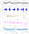 |
Fig. 2 Light curves of TOI-1430 obtained with different instruments. From top to bottom: TESS light curve (black dots) obtained from shortcadence data of sectors 14, 15, 16, 41, 54, 55, 56, 75, and 76, KELT light curve (blue crosses), STELLA light curves (green and red squares for V and I bands, respectively), Asiago Schmidt 67/92 cm u-sloan light curve (magenta squares), and LCO light curves in zs filter (azure circles). Vertical dashed lines in the upper panel indicate the gaps between the different years of the TESS mission. |
2.5 Las Cumbres Observatory
In this work, we used public archive images collected at the telescopes of the Las Cumbres Observatory (LCO). In particular, we used 284 frames collected during the night of May 24, 2021 with the 1.0 m Telescope at the McDonald Observatory, and the 292 images obtained during the night of August 6, 2022 at the 1.0m Telescope at the Teide Observatory. Both the time series were obtained with the Sinistro imager in PanStarrs zs filter and with an exposure time of 30s. In this work, we used the already prereduced images by the BANZAI pipeline (McCully et al. 2018; Xu et al. 2023).
We extracted the light curves from the LCO data with the STARSKY code (Nascimbeni et al. 2013), a software pipeline specifically designed for the TASTE project (Nascimbeni et al. 2011a) to perform differential photometry on defocused images. The size of the circular apertures and the weights assigned to each reference star were automatically set by STARSKY in order to minimise the photometric scatter of the target. More details about the STARSKY pipeline are reported in Nascimbeni et al. (2011b); Granata et al. (2014); Leonardi et al. (2024). The time stamps were consistently converted to the BJDTDB standard following Eastman et al. (2010).
2.6 HARPS-N data
TOI-1430 is one of the stars included in the GAPS Young Objects program (Carleo et al. 2020) to be monitored with HARPS-N at TNG. Observations of this star were obtained during three different seasons: the first one covered the period 1 March 2020–28 December 2020; observations during the second season were carried out between 2 May 2021 and 17 December 2021; finally, in the third season TOI-1430 was observed between 15 April 2022 and 13 November 2022. We collected a total of 191 spectra with an average S/N ~85.7 and a dispersion σ(S/N)~21.1. The average airmass and seeing conditions of the observations are 1.3 ± 0.3 and 1.2 ± 0.3 arcsec, respectively. In this work, we excluded the observation obtained during the night of 18 April 2022, because the S/N associated with the spectrum was too low (S/N ~13).
We reduced the HARPS-N spectra by using the standard Data Reduction Software (DRS) pipeline running through the YABI workflow interface implemented at the INAF Trieste Observatory1. YABI allows the HARPS-N users to run the DRS in offline mode, with the possibility to custom the reduction by changing the binary mask or the RV range to evaluate the CCF (e.g., when the target is a moderate/fast rotator). It also allows to evaluate the log R′HK activity index from the spectra collected for the RV monitoring. The RVs are extracted by using the CrossCorrelation Function (CCF) approach as specified in Pepe et al. (2002) and references therein. With this method, the observed spectrum is cross-correlated with a binary mask depicting the typical features of a specific spectral type to obtain a normalized weighted mean of the line profiles of the spectrum. In the case of TOI-1430, we used a K5 mask2. The typical value of the RV uncertainty is 0.8 m s−1. From the resulting CCF, we can measure asymmetry indices such as the Bisector Span (BIS), which is useful for tracking line profile changes due to the stellar activity. We also obtained two additional indices of the chromospheric activity, namely log R′HK and Hα. The former is directly provided by the DRS according to the methodology reported in Lovis et al. (2011) and references therein, the latter is extracted by using the ACTIN2 code (Gomes da Silva et al. 2018, 2021). The HARPS-N RV, log R′HK, Hα, and BIS time series are shown in Fig. 3 (green squares).
2.7 HIRES data
TOI-1430 was observed with HIRES (Vogt et al. 1994) on the 10 m Keck I telescope at the W. M. Keck Observatory on Maunakea.HIRES spectral range covers from 0.3 to 1.1 µm. Polanski et al. (2024) published 66 HIRES spectra of TOI-1430 obtained between 10 December 2019 and 21 October 2021 as part of the TESS-Keck Survey (TKS; Chontos et al. 2022). We subsequently obtained 47 spectra of TOI-1430 between 7 June 2022 and 14 July 2023 under the University of California and Keck observing program 2022B-U084 (PI: N. Batalha), in collaboration with the California Planet Search (CPS). All HIRES observations were obtained with a warm (50°C) cell of molecular iodine at the entrance slit (Butler et al. 1996). The superposition of the iodine absorption lines on the stellar spectrum provides both a fiducial wavelength solution and a precise, observation-specific characterization of the instrument’s PSF. The mean airmass of the observations is 1.5 ± 0.4. Across all 113 HIRES iodine-in spectra, the observations have a median exposure length of 305 s and a median S/N of 220 per pixel at 5500 Å. The majority of the observations (99 out of 113) were taken using the B5 decker (3″.75 × 0″.7861, R = 45 000), while the remaining exposures used the C2 decker (14″× 0″.7861, R = 45 000). The only difference between the two is that the length of the C2 decker enables better sky subtraction during data reduction, though this is not critical for a bright star like TOI-1430 (choosing B5 versus C2 typically makes a difference for targets with V > 10 mag). The exposures were taken with a median seeing of 1″.2 and all observations were collected with a moon separation of >30°.
To measure precise RVs using the iodine method, a high- resolution, high-S/N, iodine-free “template” spectrum must also be obtained to create a deconvolved stellar spectral template (DSST) of the host star. To compute RVs, we used the iodine- free template of TOI-1430 taken by TKS on 10 December 2019. The template was produced by averaging together two iodine- free exposures taken back-to-back. Each spectrum was collected using the B3 decker (14″× 0″.574, R = 60 000), which provides slightly higher resolution compared to the B5 or C2 deckers at the cost of throughput. The spectra were obtained at an airmass of 2.6, in seeing of 1″.1, and at a moon separation of 91°. The two template observations had exposure times of 291 s and 293 s, resulting in S/N of 215 per pixel at 5500 Åfor both. Triple-shot exposures of rapidly rotating B stars were taken with the iodine cell in the light path immediately before and after the template was collected to precisely constrain the instrumental PSF. The data collection and reduction followed the methods of the California Planet Search (CPS) as described in Howard et al. (2010).
We note here that while the HIRES template observations were obtained at a relatively high airmass, we do not find any evidence that this affects our RV measurements. Upon visual inspection, the DSST shows no signs of poor-performing deconvolution, which would typically manifest itself in the form of ripple-like features in the spectrum. Furthermore, none of the PFS fitting parameters are correlated with the measured RVs, indicating that the DSST itself is not introducing systematics into the RV measurements. Finally, the median RV precision for the HIRES data is 1.2 m s−1, which is typical for CPS observations of stars of similar spectral type.
RVs were determined following the procedures of Howard et al. (2010). As part of a forward model, the stellar spectrum was divided into about 700 pieces between ~5000–6000 Å, with each piece being 2 Å in width. For each piece, the product of the DSST and the Fourier Transform Spectrograph iodine spectrum was convolved with the PSF to match the iodine-in observation. As one of the free parameters, an RV for each piece of spectrum was produced. The pieces were weighted using all observations of the star to produce a single RV for each iodine-in spectrum. Pointwise measurement uncertainties were estimated by taking the weighted standard deviation of the mean of the velocity measured from each of the 2 Å-wide spectral chunks across all observations.
In addition to computing RVs from each spectrum, we also measured S-value activity indicators, which track Ca II H and K emission strength. The S-values were computed following the methods of Isaacson et al. (2024). The HIRES RV and log R′HK time series are shown in Fig. 3 (red circles).
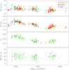 |
Fig. 3 Spectroscopic time series obtained with HARPS-N (green squares), HIRES (red circles), and APF (blue triangles) and used in this work. From the top to bottom panels: The RV, the log R′HK, the Hα, and the BIS time series. Dashed orange lines represent the fifth-degree polynomial models used for the modeling of the long trend in the spectroscopic series. The RVs have been reported in the same scale by applying an offset to them; the log R′HK series are calibrated in the same Mt. Wilson scale (Baliunas et al. 1995). |
2.8 Automated Planet Finder literature data
The TKS obtained 20 iodine-in spectra of TOI-1430 with the Levy spectrograph mounted on the 2.4 m Automated Planet Finder telescope (APF; Vogt et al. 2014) at Lick Observatory between 17 December 2019 and 27 May 2020 (Polanski et al. 2024). The observations had a median exposure time of 1800 s and a median S/N of 54 pixel−1 at 5500 Å. The observations were taken with the W decker (1″× 3″, R = 95 000).
The reduction pipeline used to compute RVs from the APF spectra mirrors the methods of Howard et al. (2010). As with the HIRES observations, spectra were obtained with a warm cell of molecular iodine in the light path. We computed the APF RVs using the iodine-free HIRES template. HIRES templates have been shown to serve as effective replacements for APF templates in the CPS Doppler reduction pipeline (e.g., Dai et al. 2020; MacDougall et al. 2021; Lange et al. 2024), and provide an efficient alternative to the long exposure that would otherwise be required to achieve similar S/N on an iodine-free APF observation. The APF RV and log R′HK time series are shown in Fig. 3 (blue triangles).
2.9 SOPHIE literature data
Four SOPHIE RVs of TOI-1430 were published by Soubiran et al. (2018), spanning from August 2008 to September 2015. The rms dispersion of these RVs is 5.6 m/s and their mean value is −27.331 km s−1, close to the mean value of HARPS-N RVs. This supports the lack of large (~ few tens m/s) variations over timescales of 15 years.
3 Stellar parameters
3.1 Kinematics and multiplicity
TOI-1430 is not associated with any known moving groups and our search, based on Gaia DR3 (see Nardiello et al. 2022, Appendix B for a detailed description) did not identify any convincing comoving objects within 5 deg, a separation much larger than any plausible physically associated companion. Oh et al. (2017) flagged the K6 star HIP 98381 as a comoving object at 673 arcmin but updated astrometry from Gaia DR3 and the highly discrepant RVs between the two stars (Soubiran et al. 2018) rule out a physical association.
TOI-1430’s position on the U,V plane is similar to that of the Hyades and well within the kinematic space of nearby young stars proposed by Montes et al. (2001). The W velocity differs by about 12 km/s with respect to that of the Hyades (see Table 1). The a posteriori probability distribution function for the kinematical age as computed from the U, V, W velocity components with the method of Almeida-Fernandes & Rocha-Pinto (2018) has a rather sharp maximum centred around ~1.3 Gyr, supporting the youthness of TOI-1430.
The similar mean RV~−27.3 km s−1 derived from SOPHIE (2008–2015) and HARPS-N (2020–2022) argues against the presence of unrecognized massive companions at a separation of a few astronomical units. This is also supported by the Renormalised Unit Weight Error (RUWE = 0.966) in Gaia DR3 and the lack of significant Gaia-HIPPARCOS proper motion anomaly (S/N ~1.52, Kervella et al. 2022).
3.2 Stellar atmospheric parameters
For the determination of stellar parameters, we considered the coadded spectrum of the target, which has an S/N ~250 at ~6000 Å. Following the same strategy as in Nardiello et al. (2022), Damasso et al. (2023), and Mantovan et al. (2024a), we inferred the atmospheric stellar parameters using the approach presented in Baratella et al. (2020) and based on equivalent widths (EW) of iron (Fe) and titanium (Ti) lines. The method was designed specifically to analyze young and intermediateage stars which show high levels of stellar activity. Briefly, it uses a combination of Fe and Ti lines to impose the excitation equilibrium for deriving Teff, and only Ti for the measurement of surface gravity log 𝑔 and microturbulence velocity ξ through ionization equilibrium and the zeroing of the trend between Ti I abundance and EW/λ, respectively. This way, we overcome possible systematic effects observed on the stellar spectra that affect the derivation of the ξ parameter, and ultimately the iron abundance (see Baratella et al. 2020 for details).
We adopted the same line list and codes as done in the works mentioned above. The EWs are measured with ARES v2 (Sousa et al. 2015), excluding those lines with EW uncertainties larger than 10% and with EW>120 mÅ. We then adopted the 1D-LTE ATLAS9 model atmospheres with the ODFNEW opacity treatment (Castelli & Kurucz 2003) and we used the 2019 version of the MOOG code (Sneden 1973) to derive the stellar parameters. Our final spectroscopic analysis indicates a Teff of 5075 ± 75 K, a log g of 4.55 ± 0.05 dex, a microturbulence ξ equal to 0.79 ± 0.07 km/s, and an iron abundance of [Fe/H] = −0.02 ± 0.03 dex and a titanium abundance[Ti/H] = 0.05 ± 0.06 dex (see Table 1). The uncertainties on iron and titanium abundances consider both the EWs scatter and the stellar parameters error contributions.
The spectroscopic results confirm with excellent agreement the values obtained using various relations exploiting Gaia DR3 photometry and parallax (Gaia Collaboration 2023) and 2MASS photometry (Cutri et al. 2003). Using the code colte (Casagrande et al. 2021), we derived the photometric values of effective temperature in 21 different color indexes, which varies from a minimum of 5048 ± 61 K (in GRP− K) up to a maximum of 5175 ± 103 K (in GRP − J), with a mean photometric Teff of 5104 ± 60 K. Given the small distance of ~42 pc from the Sun, we assumed no reddening to estimate a surface gravity of 4.58 ± 0.04 dex from the Gaia parallax and a microturbulence ξ of 0.79 ± 0.04 km/s from the relation by Dutra-Ferreira et al. (2016), again in excellent agreement with our spectroscopic values. Very close stellar parameters were also recently derived by Orell-Miquel et al. (2023) through CARMENES spectra.
Stellar properties of TOI-1430.
3.3 Lithium detection
We looked for the lithium line at 6707.8 Å in the coadded spectrum and, unlike Orell-Miquel et al. (2023), we detected a small feature, with a mean equivalent width of EWLi = 0.6 ± 0.2 mÅ. The probable disagreement with this recent work could be indeed due to the lower resolution and S /N of the coadded spectrum used by those authors, which set an upper limit of 3 mÅ for the Li EW.
However, from our stellar parameters and EW measurement, we could only obtain an upper limit of <0.1 dex on the lithium abundance with non-LTE corrections by Lind et al. (2009). This upper limit seems to be consistent with clusters not younger than the Hyades or Praesepe (~650 Myr), as also claimed by Orell-Miquel et al. (2023). Our age estimate will be discussed in Sect. 3.7.
3.4 Projected rotational velocity
As done in other previous works (see, e.g., Damasso et al. 2023; Mantovan et al. 2024a), we synthesized the absorption lines around three spectral regions (namely, 5400, 6200, and 6700 Å) to obtain an estimate of the projected rotational velocity (v sin i), after assuming the stellar parameters derived in Sect. 3.2 and fixing the macroturbulence velocity to 1.9 km s-1 from Brewer et al. (2016), the limb-darkening coefficient, and the instrumental resolution. We considered the same MOOG code and ATLAS9 grids of model atmospheres as done above and obtained a v sin i = 1.9 ± 0.6 km/s (see Table 1), which is slightly below the resolution of HARPS-N, suggesting a very slow stellar rotation unless the star is observed nearly pole-on. Similarly, Orell-Miquel et al. (2023) provided a projected rotational velocity of <2.9 km/s, which is at the limit of the resolution of their spectra.
3.5 Stellar rotation
3.5.1 Stellar rotation from photometric series
We used the light curves described in Sect. 2 to estimate the rotation period of TOI-1430. For each photometric series, we extracted the Generalized Lomb-Scargle (GLS) periodogram (Zechmeister & Kürster 2009), and we identified the period associated with the most powerful peak. Results are shown in Fig. 4: the GLS periodogram of the entire TESS light curve shows a very important peak at Prot = 11.88 ± 0.05 d (first row from the top of Fig. 4). Error on the rotation period is calculated by locally fitting a Gaussian function to the peak in the periodogram, and considering as period’s error the standard deviation. We also measured the rotation period in each of the four TESS seasons, to test any sign of differential rotation: we found Prot = 11.7 ± 0.6 d, Prot = 12.9 ± 1.8 d, Prot = 11.8 ± 0.7 d, and Prot = 11.9 ± 0.9 d for observations obtained in the years 2019, 2021, 2023, and 2024, respectively. Within the errors, all the measured rotation periods agree and no clear evidence of differential rotation is detectable from TESS data.
The second row of Fig. 4 shows the phased KELT light curve and the GLS periodogram that peaks at Prot = 11.72 ± 0.06 d with an analytical False Alarm Probability FAP~10−11. The sampling and the number of points in the STELLA light curves are not ideal for identifying the rotation period of TOI-1430; indeed, in both the photometric bands, we identified a strong peak in the STELLA GLS periodograms at Prot = 12.9 ± 0.3 d, with a FAP~0.17. The Asiago Schmidt light curve was not ideal for our purpose either, because of its low photometric precision; however, we identified a peak in the GLS periodogram at Prot = 12.13 ± 0.7 d, associated with a FAP~0.09.
3.5.2 Stellar rotation from spectroscopic series
We calculated the rotation period of the star from the HARPS-N and HIRES spectroscopic time series. As shown in Fig. 3, the log  , Hα, and BIS series show a long, sinusoidal-trend likely due to a long-period cycle of activity (P > 1000 d). To estimate the rotation period of the star we first removed this long trend by fitting a 5th-degree polynomial function to the time series characterized by coefficients shared to all the datasets and a multiplying factor associated with each time series (see, e.g., Costes et al. 2021). The fifth-degree polynomial models are shown in Fig. 3 (orange dashed line).
We extracted the GLS periodograms of all the time series (after the subtraction of the long trend) illustrated in Fig. 3, first by individually analyzing the time series obtained with the individual instruments, and then by considering all the points at once. Periodograms are shown in Fig. 5: from the HARPS- N RV, log  , Hα, and BIS series we observed a peak in the periodogram at Prot = 11.85 ± 0.12 d (FAP~10−4), Prot = 11.67 ± 0.11 d (FAP~10−7), Prot = 11.85 ± 0.09 d (FAP~10−8), and Prot = 11.51 ± 0.17 d (FAP~10−5), respectively (see the five topper panels of Fig. 5). The HIRES RV and log
  series periodograms show a peak at Prot = 12.05 ± 0.11 d (FAP~2 × 10⁻³) and Prot = 12.45 ± 0.26 d (FAP~7 × 10⁻³) (bottom panels of Fig. 5). Analysing the complete RV time series we obtained Prot = 11.85 ± 0.09 d(FAP~3 × 10⁻⁷).
Averaging all the Prot estimated from photometry and spectroscopy, we obtained a weighted average rotation period Prot = 11.9 ± 0.3 d.
3.6 Coronal and chromospheric activity
The chromospheric activity S-index was measured on the spectra as described in Sect. 2. The median value from the HARPS-N time series is ~0.480, that is log  , derived adopting (B−V) = 0.888 from Teff = 5090 K, as the observed B–V color has large uncertainty.
TOI-1430 has an X-ray detection (1RXS J200226.3+532229) within 15 arcsec from the optical position on ROSAT Faint Source Catalog (Voges et al. 2000). The corresponding X-ray luminosity, derived following Hünsch et al. (1999), is LX = 2.44 × 1028 erg s−1, and the ratio log LX/Lbol ≃ −4.76. More recently, the object was the target of XMM-Newton observations (Zhang et al. 2023). The analysis of this observation by Orell-Miquel et al. (2023) yielded LX = 1.89 ± 0.07 × 1028 erg s-1 in the band 5–100 Å, corresponding to log LX/Lbol ≃ −4.86. Both log  and LX/Lbol are below the mean value for Hyades stars of similar color, but in agreement with the predictions of these emission levels based on the stellar age and rotational period (Pizzolato et al. 2003; Mamajek & Hillenbrand 2008). In particular, the X-ray luminosity is below the 1σ lower boundary of the dispersion for the members of the Hyades cluster observed in X-rays (Penz et al. 2008).
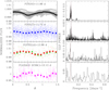 |
Fig. 4 Analysis of the rotation period of TOI-1430 performed with different photometric series. The left panels show the light curves folded with the period associated with the peak of the corresponding GLS periodogram (right panels). Φ is the rotational phase of the star. From the upper panel to the bottom, we report the analysis carried out on TESS, KELT, STELLA, and Asiago Schmidt light curves, respectively. |
3.7 System age
The rotation period, lithium abundance, coronal and chromospheric emission are all consistent with an age similar and probably slightly older than the Hyades. The kinematic properties are also fully compatible with such an age value but there are no known companions or comoving objects to further refine the age determination. Therefore, considering the measurement uncertainties and the scatter in the indicators for coeval objects, we adopt an age of 700 ± 150 Myr. Our adopted age is significantly older than that adopted by Zhang et al. (2023) (165±30 Myr), as they obtained a rotation period which is roughly half of our determination and consider only gyrochronology for dating the star. Our age determination is instead in good agreement with the findings by Orell-Miquel et al. (2023) and Filomeno et al. (2024) (600–800 Myr), based on a combination of various methods, similar to our adopted procedure3. As noticed also by Orell-Miquel et al. (2023), the expected lithium abundance for the age by Zhang et al. (2023) is highly discrepant with the observational value, ruling out such a young age.
3.8 Stellar radius and mass
Stellar radius was obtained from Stefan-Boltzmann law, using the adopted Teff, the observed V mag from HIPPARCOS, and the bolometric correction from Pecaut & Mamajek (2013)4. The stellar luminosity results in 0.360±0.026 L⊙ and the stellar radius 0.772±0.029 R⊙.
Stellar mass was obtained using the PARAM web interface (da Silva et al. 2006)5 which interpolated the models by Bressan et al. (2012), in a Bayesian framework to identify the most probable solution considering the observational errors and the lifetime of the various evolutionary phases. Only the age range derived by indirect methods was allowed in the retrieval, as in Desidera et al. (2015), considering the evolutionary timescales of an early K dwarf. The stellar mass results 0.849±0.009 M⊙. The small uncertainty is only due to the contribution of the “internal” error of the fitting procedure, while systematic uncertainties of the stellar models are not included; for this reason we increased the error on the prior on stellar density in subsequent analyses. The mass and radius agree to be better than one sigma with Orell-Miquel et al. (2023), Zhang et al. (2023), and TESS Input Catalog (TIC, Stassun et al. 2018, 2019).
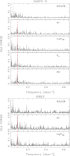 |
Fig. 5 Analysis of the rotation period of TOI-1430 carried out on the HARPS-N (five upper panels) and HIRES (three bottom panels) spectroscopic series shown in Fig. 3 (after the subtraction of the long trend). Panels show the GLS periodograms extracted from the RV, log |

4 Detection and vetting of TOI-1430 b
A transiting object in the light curve of HD 235088 was detected by the Science Processing Operations Center (SPOC) pipeline (Jenkins et al. 2016) in November 2019, and was assigned to the identifier TOI-1430.01. Through a statistical analysis, Giacalone et al. (2021) found a false-positive probability (FPP) of ~0.03 for the transit signals, labeling this object as a likely planet. In this section, we provide further evidence of the planetary nature of this object.
First, we detrended the light curve of TOI-1430 using the Tukey’s biweight M-estimator implemented in wōtan (Hippke et al. 2019), with a window length of 1 day. To obtain the model, we masked the likely transit events by using the ephemeris given by the SPOC pipeline. The detrending model is shown in red in panel a of Fig. 6. We extracted the Transit Least Squares (TLS) periodogram (Hippke & Heller 2019) of the detrended light curve (panel b of Fig. 6), looking for transit signals with periods between 1 and 100 days: the periodogram illustrated in panel d of Fig. 6 shows a peak at P ~ 7.434 d with a Signal Detection Efficiency (SDE) of ~91.1, and a stacked S/N ~21.3. Odd and even transits are reported with magenta and blue triangles in panel b, respectively. We checked if the depths of the odd/even folded transits agree; the results are reported in panels c. The significance (in standard deviations) between odd and even transit depths is ~0.4; that is, odd and even transits have on average the same depth within ~0.4σ. We also tested the in-/out- of-transit centroid associated with the signal of the transiting object as described in Desidera et al. (2023) and Maldonado et al. (2023). The result is shown in Fig. 7: all the centroids, each one calculated as the average of the in-/out-of-transit centroids of each sector, agree within the errors with the position of TOI- 1430. Finally, we also checked if there is any correlation between transits and (X,Y) positions of the star on the CCD and between transits’ depths and different photometric apertures. The transiting object passed positively all the vetting tests and we confirmed its planetary nature (hereafter TOI-1430 b).
We masked the transit events of the planet TOI-1430 b from the detrended light curve, and we extracted three TLS periodograms to look for other transit features. In the first TLS periodogram, we sampled all the periods between 0.45 d and 1.0 d, in the second periodogram all the periods between 1.0 d and 10.0 d, and finally in the third periodogram we looked for transit signals with periods between 10.0 and 100.0 d. We did not obtain any strong peaks in the periodograms. Indeed, in the first case, we measured a peak at period P~ 0.85 d with an SDE~ 0.09 and S/N ~ 1; in the second case the peak in the periodogram corresponds to P ~ 7.04 d (SDE~12, S/N ~3.5); finally in the third case we obtained a peak in the TLS periodogram at P ~ 84.6 d with an SDE~11 and S/N ~ 8.5. Inspecting the folded light curve with the recovered periods, no evidence of transits is visible.
5 The planetary system of TOI-1430
In this section, we present the modeling of the TESS light curve and of the RV series in order to characterize TOI-1430 b. We used the publicly available code PyORBIT6 (Malavolta 2016; Malavolta et al. 2016, 2018), a versatile public available software for the characterization of planetary systems that is able to model stellar activity, planetary signals, and instrumental systematics in the light curves, RV and activity index series, also adopting Gaussian processes regression with a variety of kernels. This code has been successfully adopted in many works under the GAPS Young Objects program (see, e.g., Mantovan et al. 2024a; Carleo et al. 2024). It firstly derives the starting values of the parameters used in the fit of the models by executing the algorithm PyDE7 (Storn & Price 1997), a global optimization code ideal to obtain the starting conditions. Secondly, these starting parameters are then used to initialize the affine invariant Markov chain Monte Carlo (MCMC) sampler emcee (Foreman-Mackey et al. 2013).
We analyzed the detrended light curve shown in panel b of Fig. 6 and the spectroscopic series shown in Fig. 3 with PyORBIT in order to retrieve the planet’s properties. We adopted as Gaussian priors the stellar parameters (stellar mass and radius, M⋆ and R⋆, respectively) reported in Table 1 as input; however, to take into account that the error on the stellar mass is underestimated, we adopted a broader prior on the stellar density.
We modeled the transits by using the package batman8 (Kreidberg 2015) in order to retrieve information on the central time of the first transit (T0,b), the orbital period (Pb), the impact parameter (bb), the planetary-to-stellar-radius ratio (RP,b/R⋆), the duration of the transit (T14,b, calculated as in Winn 2010) the stellar density (ρ⋆), and the photometric jitter term (σjit,phot) to be added in quadrature to the errors of the photometry to take into account any systematic or physical residual effects we did not corrected. We took into consideration the contamination of the neighbor stars that fall inside the photometric aperture, and we calculated the dilution factor (d f = 0.0073 ± 0.0002) that we used as Gaussian prior in the modeling. Also, by adopting the [Fe/H], log 𝑔 and Teff shown in Table 1, we calculated the coefficients of limb darkening (LD) using the routine PyLDTk9 (Husser et al. 2013; Parviainen & Aigrain 2015), increasing the errors of a factor 10 in the priors in order to avoid deviations between the measured and predicted LD coefficients. During the modeling, we adopted the LD formalism by Kipping (2013) and we took into account the 2-minute cadence of the light curve (Kipping 2010). Priors for the planet transit modeling, chosen on the basis of the analysis performed in the previous sections, are reported in Table 2.
We used PyORBIT to simultaneously model the stellar activity and the planetary signal in the RV time series and the stellar activity signal in the log  , Hα, and BIS series. Stellar activity was modelled through the multidimensional Gaussian process (GP) framework. In this work, we made use of the tinyGP10 routines for the GP regression, that works also on GPUs11. The multidimensional GP is implemented in PyORBIT following the prescription of the work by Rajpaul et al. (2015) (see Barragán et al. 2022a for details). We modeled the RV, log
  , BIS, and Hα spectroscopic time series. The four-dimensional GP model is described by the following equations:
 (1)
(1)
 (2)
(2)
 (3)
(3)
 (4)
(4)
where G(t) and Ġ(t) are the underlying GP and its derivative, with the quasi-periodic kernel described by:
![Mathematical equation: $\gamma \left( {{t_i},{t_j}} \right) = \exp \left\{ { - {{{{\sin }^2}\left[ {\pi \left( {{t_i} - {t_j}} \right)/{P_{rot}}} \right]} \over {2{w^2}}} - {{{{\left( {{t_i} - {t_j}} \right)}^2}} \over {2P_{dec}^2}}} \right\},$](/articles/aa/full_html/2025/01/aa52236-24/aa52236-24-eq15.png) (5)
(5)
where Prot is the GP period equivalent to the stellar rotation period, w is the coherence scale, and Pdec is associated with the decay timescale of the active regions. The constants Vc, Vr, L1c, Bc, Br, and L2c are free parameters that link the individual time series to the GP and its derivative (Nardiello et al. 2022; Barragán et al. 2023). To take into account the different data reduction and instrument properties, we treated observables coming from different observatories as independent datasets, with their own offset and jitter parameters We adopted a Gaussian prior on the stellar rotation equal Prot = 11.9 ± 0.3 d, on the basis of the results obtained in Sect. 3.5. We explored the period and the semi-amplitude of the planet in linear space, and we imposed the eccentricity equal to 0. The priors adopted are shown in Table 2.
After running the global parameter optimization routine PyDE, we adopted 8 × ndim walkers (where ndim is the dimensionality of the model) to run the sampler with the standard ensemble method (Goodman & Weare 2010) for 120 000 steps, excluding the first 30 000 as burn-in. To reduce the effect of the chain autocorrelation, we adopted a thinning factor of 100. We adopted the Gelman-Rubin statistics and the auto-correlation analysis to check the convergence of the chains.
All the results are reported in Table 2. Figure 8 shows the activity modelling for all the available time series, and the modelling of TOI-1430 b in both the photometric and RV series.
We also tested the case with non-null eccentricity, finding similar results, as shown in Table 2, and an eccentricity of  , which is consistent with zero. We again ran the analysis .of cases with e = 0 and e ≠ 0 using the dynamic nested sampling algorithm implemented in the package dynesty (Buchner 2016; Higson et al. 2019; Speagle 2020) both to check the consistency of the results of the posteriors distributions of the planet parameters, and to calculate (and compare) the Bayesian evidence log 𝒵 to evaluate the quality of the fits in the two cases. The obtained results for the stellar activity and planet parameters are consistent with those obtained with emcee. In the case of circular orbit, we obtained a log 𝒵 ≃ 299.2, while in the case of Keplerian orbit log 𝒵 ≃ 297.2. Even if the difference in log 𝒵 between the models is not significant (Δ log 𝒵 ~ 2), the case of a circular orbit is preferred. We note that even assuming a strong tidal dissipation in the solid core of the planet (see Sect. 6 for internal models) as parameterized by a modified tidal quality factor
  (Henning et al. 2009), the decay time of the eccentricity is e/|de/dt| ~ 0.9 Gyr that is not short in comparison with the estimated age of the system. Therefore, any primordial eccentricity should not have been reduced by tides by more than a factor of 2–3 suggesting that the initial orbit was not remarkably eccentric.
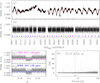 |
Fig. 6 Detection and vetting of the candidate exoplanet TOI-1430.01. Panel a shows the stacked light curve of TOI-1430 and the detrending model (in red). Panel b shows the flattened light curve and the position of the odd (magenta) and even (blue) transits. Panels c are a comparison between the mean depths of the odd and even transits; the dashed lines are the mean depths while the shaded colored regions represent the 3σ confidence interval. Panel d is the TLS periodogram: the period of the peak is indicated with a green triangle. |
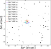 |
Fig. 7 In-/out-of-transit centroid analysis for TOI-1430.01. TOI-1430 is centered on (0,0). Black filled circles are the neighboring stars from Gaia DR3; the dimensions of the points are proportional to the apparent luminosity of the stars. Each colored point corresponds to the average of the centroids in each sector. Within the errors, centroids match with the position of TOI-1430. |
5.1 Searching for other planets
We investigated the presence of a second, non-transiting planet in the RV dataset. We limited the analysis to the spectroscopic series, giving a strict prior on the period of planet b on the basis of the previous analysis (but leaving free the RV semi-amplitude).
To check the presence of a second planetary signal, we run PyORBIT again adopting the multidimensional GP framework for the modeling of the stellar activity, which is less sensitive to overfitting problems of the spectroscopic series. By using the same priors of Table 2, chains converged for Pc ~ 96.4 d (that is ~8 × Prot) and Kc ~ 1.3 m/s (~4σ detection). We restricted this analysis to sampling orbital periods in the interval 0.4 ≤ Pc ≤ 20.0 days; the result was a signal at Pc ~ 12.68 d and Kc ~ 1.3 m/s (~4σ detection).
The disagreement between the results obtained with different models of stella r activity (see also Appendix E) suggests that the measured signal of candidate planet c is probably due to residuals in the fit of the stellar activity, which turns out to be quite difficult to model.
For the sake of completeness, we report in Fig. E.1 and Table E.1 all the results related to these signals; more data and analysis are mandatory to confirm their planetary nature.
Stellar activity with multidimensional GP and parameters of TOI-1430 b.
 |
Fig. 8 Overview of the modeling that uses the multidimensional GP for the stellar activity. From the top, the first four panels show the RV, log |

5.2 Analysis of transit timing variations
We investigated the presence of dynamical interactions of TOI- 1430 b with other potential bodies in the system. In order to perform this analysis, we calculated the transit timing variations (TTVs, Agol et al. 2005; Holman & Murray 2005) as the difference between the observed central times of the transits (O) and the computed central times of the transits (C) from the linear ephemeris (Table 2). We modeled every single transit by using PyORBIT. In this analysis, we also included the two groundbased light curves collected with LCO. The modeling of single transits is reported in Fig. F.1. Figure 9 shows the O–C diagram.
The possible TTV amplitude, that is, the semi-amplitude of the O–C series, is ATTV ≃ 7.7 minutes. To check if there is any hint of TTV we calculated the χ2 of the linear ephemeris fitting as:
 (6)
(6)
where N is the number of available epochs for which we calculated the central times of the transits, and σ+ and σ− are the positive and negative errors associated with the O–C. We obtained χ2 ~ 9.4 and a reduced  , where 32 are the degrees of freedom. The linear ephemeris fits well the data and there is no hint of TTV. In Table F.1 the T0 values for the different epochs are reported.
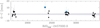 |
Fig. 9 Analysis of TTVs based on TESS and LCO data. The figure shows the O–C plot of the observed (O) and calculated (C) transit times for the linear ephemeris of TOI-1430 b. |
6 Results
6.1 System inclination
The combination of the measured stellar rotation period, projected rotational velocity (Sect. 3.4, Table 1), and stellar radius (Table 1) yield a stellar inclination of  deg. The equatorial velocity implied by stellar rotation period and stellar radius is 3.28±0.17 km s−1. The possibility that the true rotation period is two times the observed one (double-dip behavior) can be dismissed considering the levels of chromospheric and coronal activity, which are fully consistent with the adopted rotation period, derived from both spectroscopic and photometric time series. Therefore, there are indications that the star rotation is not aligned with the planetary orbit, although this needs to be confirmed through measurement of the Rossiter–McLaughlin effect (Queloz et al. 2000, expected maximum amplitude ~1 m s−1). Tides induced by the planet in the star are not sufficiently strong to modify the obliquity of the orbit because of the small mass of the planet. Therefore, the current obliquity should be close to the primordial obliquity of the system.
6.2 Mass–radius diagram
In this work, we have measured the mass and the radius of the exoplanet TOI-1430 b with an high-level of precision (~19% and ~4%, respectively). In Fig. 10 we report the results in the mass– radius diagram, where all other young planets (<1 Gyr) with accurate (based on different techniques) and precise (relative errors <50%) age measurements are also reported. Combining the values reported in Tables D.1 and 2, we obtained a planetary density of ~0.53ρ⊕ ~ 3 g cm−3. The low density of this exoplanet is due to its extended atmosphere; the detection of an escaping atmosphere is reported by Zhang et al. (2023) and Orell-Miquel et al. (2023): both the works reported the detection of helium excess absorption (~−0.6 to −0.9%) due to the atmosphere of TOI-1430 b. It is among the few small planets with a robust detection of the atmosphere.
As shown in Fig. 10, TOI-1430 b is located at the upper limit of the “radius gap” (Fulton et al. 2017; Fulton & Petigura 2018), that region in the mass–radius diagram sparsely populated by exoplanets that divides the rocky Earths/super-Earths from the low-density mini-Neptunes. This gap could be an effect of the atmospheric evolution of mini-Neptunes characterized by a rocky core and an extended H/He atmosphere that inflates their radius. This atmosphere is then stripped away through mechanisms such as photo-evaporation (Owen & Wu 2013, 2017) or core-powered mass loss (Ginzburg et al. 2018), resulting in the exposure of the rocky core, as in the rocky planets we observe today below the radius gap.
By comparing the derived planet parameters with the tracks by Zeng et al. (2019)12, it results that TOI-1430 b is compatible with an Earth-like rocky core (32.5% Fe+67.5% MgSiO3) + 0.3% H2 atmosphere/envelope, or with a water world (50% Earth-like rocky core + 50% H2O). Also, the comparison of the mass and radius of TOI-1430 b with the 700 Myr old tracks calculated by Lopez & Fortney (2014) is in agreement with a planet with a 0.2–0.5% H/He envelope. The atmospheric evolution model described in the next section, based on the assumption the planet is a rocky world with an extended atmosphere, predicts that in ~200 Myr this planet will lose its envelope showing its ~1.5 R⊕ rocky core, as illustrated by the arrow in Fig. 10.
6.3 TOI-1430 b atmospheric evolution
Given its young age (700 ± 150 Myr), TOI-1430 b represents a prime target for photo-evaporation studies. To assess the current atmospheric mass loss rate, the past history and the fate of the TOI-1430 b atmosphere subjected to photo-evaporation, we followed a modeling approach proposed by Locci et al. (2019), which has been used and updated in several previous works (e.g., Benatti et al. 2021; Maggio et al. 2022) and most recently described in detail by Mantovan et al. (2024b). In brief, we coupled the new ATES photoionization hydrodynamics code (Caldiroli et al. 2021, 2022; Spinelli et al. 2023) with the planetary core-envelope models by Fortney et al. (2007) and Lopez & Fortney (2014), the MESA Stellar Tracks (MIST; Choi et al. 2016), and the XUV luminosity time evolution by using different prescriptions (Penz et al. 2008; Sanz-Forcada et al. 2022; Johnstone et al. 2021).
Simulating a grid of exoplanets with different levels of X-ray and Extreme Ultraviolet (XUV) irradiation and different gravitational potential energy, Caldiroli et al. (2022) found an analytical approximation for the evaporation efficiency, ηeff. Using this evaporating efficiency as a function of the gravitational potential energy of the planet and the XUV irradiation in the classical energy-limited formula (Erkaev et al. 2007), it is possible to derive an approximation of the atmospheric mass loss rate evaluated with hydrodynamic simulations:
 (7)
(7)
where FXUV is the XUV flux at the (average) orbital distance, Ψ the gravitational potential energy of the planet, ρp is the mean planetary mass density and the factor K accounts for the host star tidal forces (Erkaev et al. 2007). We used this analytical approximation to speed up the modeling of the past and future evolution of the planet.
We considered the stellar bolometric and XUV luminosity evolution. We obtained the stellar evolutionary track (the theoretical temperature-luminosity diagram shown in Fig. 11) through the web-based interpolator13 of the MESA Isochrones and Stellar Tracks (MIST, Choi et al. 2016).
We assumed two different descriptions to estimate the evolution of stellar X-ray and EUV emission. The first method is the X-ray luminosity versus age analytical relation for G-type stars derived by Penz et al. (2008), anchored to the current value of the X-ray luminosity (Sect. 3.6). In this case, to estimate the stellar irradiation in the EUV band, we used the scaling law between EUV (100–920 Å) and X-ray (5–100 Å) luminosities, derived by Sanz-Forcada et al. (2022):
 (8)
(8)
In Fig.12, we show with red lines the predicted evolution of the X-ray and EUV stellar luminosities obtained with this method.
The second method that we adopted to model the evolution of TOI-1430 X-ray and EUV emission is the semi-empirical modeling by Johnstone et al. (2021), where the X-ray to bolometric luminosity ratio, LX/Lbol follows a broken power law with the Rossby number (Pizzolato et al. 2003; Wright et al. 2011), i.e that is the ratio of the rotation period to the convective turnover time. In this case, the initial rotation rate of the star at early ages (Ω0 at t = 1 Myr) determines the evolutionary track of Lx/Lbol in time, for any star with a given mass. For TOI-1430 we selected the track of a star with M* = 0.85 M⊙ which predicts the X-ray luminosity nearest to the measured value, at an age in the range 550–850 Myr. Then, we computed the EUV luminosity following again Johnstone et al. (2021), who proposed an empirical mass-independent power-law scaling between the surface EUV and X-ray fluxes calibrated on a sample of stars observed with the Extreme Ultraviolet Explorer satellite and solar spectra derived from the TIMED/SEE mission. The X-EUV luminosity tracks derived with this second method are also shown in Fig.12 with blue lines.
It must be noted that the actual (measured) LX value (Sect. 3.6) remains lower than the emission level expected in both the descriptions by Penz et al. (2008) and Johnstone et al. (2021). According to the latter, the expected X-ray luminosity for the stars with the lowest activity level should be about 4 × 1028 erg s−1 (Fig. 12), corresponding to a Rossby number  (Wright et al. 2018), that is more than a factor 2 higher than the observed LX value. In other words, TOI-1430 appears to have a high-energy emission level relatively lower than expected for stars with similar mass and age, such as the members of the Hyades open cluster.
Assuming the planetary parameters in Table 2, the mass loss rate estimated by running the ATES hydrodynamic simulation gives a value between 3.1–3.5 × 10¹⁰ g s−1 depending on the XUV prescriptions (Johnstone et al. 2021 and Sanz-Forcada et al. 2022 respectively). This value is consistent with the estimation performed by Orell-Miquel et al. (2023) (1.5–5 ×10¹⁰ g s−1), who used the 1D hydrodynamic model by Lampón et al. (2020).
To evaluate the past and the future evolution of the planetary atmosphere subjected to photoevaporation we determined the planetary core mass, the atmospheric mass fraction and the radius at the current age by adopting the core-envelope model described in Lopez & Fortney (2014). This core–envelope model has four unknowns: the mass and radius of the core, Mcore and Rcore , the radius of the envelope, Renv , and the atmospheric mass fraction, fatm . Four relations and two observational constraints link these quantities: the measured planet radius and total mass, Rp and Mp; the Lopez & Fortney (2014) relation which links Renv, fatm, and Mp ; and a relation between Rcore , Rp , and Mp at the given age and star–planet distance. For the latter, we adopted the internal structure models by Fortney et al. (2007), where cores can be composed of different ice–rock or rock–iron mixtures.
We note that the relation by Lopez & Fortney (2014) was developed for atmospheres dominated by H–He, and also takes into account the cooling and contraction of the envelope as a consequence of its thermal evolution (Lopez et al. 2012). In the Lopez & Fortney (2014) relation, the radius time dependence is linked to the metallicity. For atmospheres with solar opacity, the radius of the envelope decreases with age as ∝ t−0.11, while for an enhanced opacity, the variation is ∝ t−0.18. Allowing for the time variation of bolometric luminosity and surface temperature equilibrium introduces a further time dependence on the envelope size.
Assuming an Earth-like core composed of 67% rocks and 33% iron, and an envelope with solar opacity, we found for TOI-1430-b a solution with Mcore,b = 4.13 M⊕, Rcore,b = 1.45 R⊕, Renv,b = 0.53 R⊕, and fatm = 0.42%, corresponding to the measured planetary mass and optical radius. With an enhanced metallicity envelope we found another solution with Mcore,b = 4.14 M⊕, Rcore,b = 1.45 R⊕, Renv,b = 0.53 R⊕, and fatm = 0.33%.
We then proceeded with the time evolution of the photoevaporation. For each time step of the simulation, we computed the mass-loss rate and updated fatm and the planetary mass, obtaining a new value of Renv with the relation by Lopez & Fortney (2014). The latter quantity added to the core radius (assumed constant) provides the updated planetary radius.
According to the aforementioned scenario and assuming a core that does not change in size or mass, we followed the planetary evolution back in time. We stopped our simulations in the past at 3 Myr, the end time of planetary formation models, that is, when the circumstellar disk has already disappeared and each planet is in its final, stable orbit. For future evolution, we let the system evolve from the current age (700 Myr) until 5 Gyr. The results of the simulations dependent on different assumptions are shown in Fig. 13.
Currently, the planet is close the radius gap (Fulton et al. 2017) with a radius of 1.982 R⊕. As shown in Fig. 13, our model shows that the planet experienced significant evolution in the past, from a birth as a (super-)puffy planet to the current sub-Neptune properties.
In order to retain a part of this envelope at the current age (700 Myr, an envelope mass fraction of ~0.3–0.4%) our model suggests that the planet was surrounded by a very large envelope at the beginning of its evolution. More specifically, the model with a solar-opacity envelope suggests an envelope mass fraction at 3 Myr of 29% or 21%, assuming the Sanz-Forcada et al. (2022) or Johnstone et al. (2021) XUV evolution, respectively. The corresponding planetary radius was 12.7 R⊕ or 11.0 R⊕, with a planetary mass of 5.9 M⊕ or 5.3 M⊕. The model with an enhanced-opacity envelope suggests an even larger envelope. Assuming the Sanz-Forcada et al. (2022) XUV evolution, this model predicts an envelope mass fraction at 3 Myr of 59%, with a radius of 26.8 R⊕ and a mass of 10.0 M⊕, while assuming Johnstone et al. (2021) the envelope mass fraction was 51%, with a planetary radius of 25.7 R⊕ and a planetary mass of 8.5 M⊕. At 3 Myr the exoplanetary mass loss rate was in the range 5.8–11.1 × 10¹² g s−1 for the solar-opacity model, and 6.5–8.2 × 10¹³ g s−1 for the enanched-opacity envelope model.
Under the effect of photoevaporation, the planet lost much of its envelope in the first 300 Myr under the effect of high-energy stellar irradiation. At 300 Myr the envelope mass fraction was between 3.6% and 6.1% depending on the different assumptions that we adopted, with a planetary radius and a planetary mass between 3.5–4.9 R⊕ and 4.3–4.4 M⊕, respectively.
Regarding the future of the planet, our model predicts that it will completely lose its envelope in the next 150–200 Myr, and it will become an envelope-stripped super-Earth-size planet with a radius equal to the core radius (1.48 R⊕). Our simulations show that the planet undergoes a noticeable radius evolution. In fact, the planet started its evolution as a Jovian or puffy-Jovian (depending on the model). Between around 100 and 600 Myr, it passed through the first peak of the bimodal distribution, reaching its current position at the edge of the Fulton gap. Within the next hundreds of Myr, the planet will completely lose its atmosphere, crossing the Fulton gap and ending its evolution as a Chthonian planet in the second peak of the distribution.
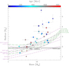 |
Fig. 10 Mass–radius diagram for young (<1 Gyr) planets with precise age estimates (relative errors <50%). TOI- 1430 b is located at the edge of the Fulton gap; the arrow indicates the final position in the diagram in the next 200 Myr, when it will completely lose its atmosphere. The Zeng et al. (2019) tracks are reported in magenta (dot-dashed lines) in the case of planets composed of 100% Fe, 32.5% Fe+67.5% MgSiO3 (Earthlike), 50% Earth+50% H2O, and 99.7% Earth+0.3% H2; the Lopez & Fortney (2014) tracks for exoplanets with H/He envelopes between 0.01% and 1% are reported in green. Exoplanets with accurate age estimation are color-coded on the basis of the color bar at the top of the figure; square points are the exoplanets with accurate mass measurement, and triangles are the exoplanets with a mass upper limit measurement. |
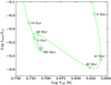 |
Fig. 11 Evolutionary track of TOI 1430 in the effective temperature- bolometric luminosity plane. A gray dot marks the current location of the star on the track. |
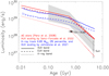 |
Fig. 12 Time evolution of X-ray (5–100 Å), EUV (100–920 Å), and total XUV luminosity of TOI 1430, according to Penz et al. (2008) and the X-ray/EUV scaling by Sanz-Forcada et al. (2022) (red lines) and according to Johnstone et al. (2021) (blue lines). Uncertainties on the age and X-ray luminosity of TOI 1430 are also indicated. The gray area is the original locus for dG stars in Penz et al. (2008). |
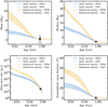 |
Fig. 13 Evolution of the planetary mass (upper-left panel), planetary radius (upper-right panel), atmospheric mass-loss rate (bottom-left panel), and atmospheric mass fraction (bottom-right panel) according to our models with different assumptions. Black squares mark the current location of the star in each plot. |
7 Conclusions
In this work, we measured the density of the young planet TOI- 1430 b with high precision thanks to the combination of exquisite data sets provided by TESS, HARPS-N, HIRES, and APF instruments. First, we derived the stellar parameters adopting information from Gaia and analyzing complementary spectroscopic and photometric data. In particular, on the basis of the stellar rotation period (Prot ~ 12 d), the kinematics, the lithium abundance, and the coronal and chromospheric activity, we find that TOI-1430 is 700 ± 150 Myr old.
We combined the TESS light curves of nine sectors with spectroscopic series collected with HARPS-N@TNG, HIRES@Keck, and APF in a ≳3 year campaign to simultaneously model the activity and the signal of the planet. To model the stellar activity in the spectroscopic series we adopted two different approaches: (i) GP regression with a quasi-periodic kernel, and (ii) a multidimensional GP framework. Planet parameters are reported in Table 2. We measured a stellar rotational period of Prot = 12.2 ± 0.1 d and a planetary mass of MP,b = 4.2 ± 0.8 M⊕ . The planetary radius we measured is RP,b = 1.98 ± 0.07 R⊕. From these values, we inferred a density of ρb ∼ 0.53 ± 0.12 ρ⊕ = 2.9 ±0.7 g cm−3, meaning TOI-1430 b is a low-density mini-Neptune with an extended atmosphere located at the upper edge of the radius gap in the mass–radius diagram (see Fig. 10).
Zhang et al. (2023) and Orell-Miquel et al. (2023) detected an evaporating He atmosphere around TOI-1430 b. By adopting the planet parameters derived in this work, we traced the history of the atmosphere of this planet, from 3 Myr after its birth to the present age and also for the next 5 Gyr. We find that the planet’s radius has significantly evolved during its lifetime: starting from a Jovian/puffy-Jovian (~10–25 R⊕ and ~5–10 M⊕, on the basis of the model adopted), the planet lost most of its envelope in the first 100–300 Myr. With a radius of ~2 R⊕, the planet is presently entering the Fulton gap and continues to lose its atmosphere. In the next 100–200 Myr, TOI-1430 b will lose its entire envelope, becoming an Earth-size rocky planet of ~1.5 R⊕.
Data availability
HARPS-N, HIRES, and APF spectroscopic time series used in this work are available at the CDS via anonymous ftp to cdsarc.cds.unistra.fr (130.79.128.5) or via https://cdsarc.cds.unistra.fr/viz-bin/cat/J/A+A/693/A32.
Acknowledgements
The authors thank the anonymous referee for helping to improve the quality of the paper. This work has been supported by the PRIN- INAF 2019 “Planetary systems at young ages (PLATEA)” and ASI-INAF agreement no. 2018-16-HH.0. V.N., G.P., L.M. acknowledge financial support from the Bando Ricerca Fondamentale INAF 2023, Data Analysis Grant: “Characterization of transiting exoplanets by exploiting the unique synergy between TASTE and TESS”. A.M. acknowledges partial support by the project HOT-ATMOS (PRIN INAF 2019), and by the PRIN/MUR EXO-CASH. R.S. acknowledges the support of the ARIEL ASI/INAF agreement no. 2021-5-HH.0 and the support of grant no. 2022J7ZFRA – Exo-planetary Cloudy Atmospheres and Stellar High energy (Exo-CASH) funded by MUR -– PRIN 2022. L.M. acknowledges financial contribution from PRIN MUR 2022 project 2022J4H55R. We acknowledge the Italian center for Astronomical Archives (IA2, https://www.ia2.inaf.it), part of the Italian National Institute for Astrophysics (INAF), for providing technical assistance, services and supporting activities of the GAPS collaboration. This work includes data collected with the TESS mission, obtained from the MAST data archive at the Space Telescope Science Institute (STScI). Funding for the TESS mission is provided by the NASA Explorer Program. STScI is operated by the Association of Universities for Research in Astronomy, Inc., under NASA contract NAS 5–26555. We acknowledge the use of public TESS data from pipelines at the TESS Science Office and at the TESS Science Processing Operations Center. Resources supporting this work were provided by the NASA High-End Computing (HEC) Program through the NASA Advanced Supercomputing (NAS) Division at Ames Research Center for the production of the SPOC data products. Funding for the TESS mission is provided by NASA’s Science Mission Directorate. This work has made use of data from the European Space Agency (ESA) mission Gaia (https://www.cosmos.esa.int/gaia), processed by the Gaia Data Processing and Analysis Consortium (DPAC, https://www.cosmos.esa.int/web/gaia/dpac/consortium). Funding for the DPAC has been provided by national institutions, in particular the institutions participating in the Gaia Multilateral Agreement. This work makes use of observations collected at the Asiago Schmidt 67/92 cm telescope (Asiago, Italy) of the INAF -– Osservatorio Astronomico di Padova. This paper made use of data from the KELT survey (Pepper et al. 2007).
Appendix A Light curve correction
In Fig. A.1 we compare the light curves of TOI-1430 extracted with the PATHOS and the official pipelines. The need to extract the light curves with a different pipeline arises from two different reasons: (i) from SAP to PDCSAP light curves any original information on the stellar variability is compromised, as demonstrated in panel (a); (ii) the presence of a positive signal in the SAP light curves (P~2.81 d) due to a close-by eclipsing binary and bad estimation of the local background (panels (b) and (c)).
In the PATHOS pipeline, the photometry of the stars is extracted after the subtraction of neighbor contaminants that are modeled by using an input catalog (Gaia DR3) and the TESS PSF models. The local background is measured by using the pixels inside an annulus with inner radius 6 pixel and outer radius 20 pixel and centered on the target star. To avoid the contamination of potential variable stars (like the eclipsing binary TIC 293954660) in the calculation of the local background, the PATHOS routine masks the pixels corresponding to the location of the neighbor stars (on the basis of the Gaia DR3 catalog) and where the contribution of neighbors’ PSF is >0.1%.
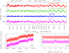 |
Fig. A.1 Comparison between the PATHOS and official TESS light curves of TOI-1430. Panel (a) shows the SAP and the PDCSAP light curves (in magenta and blue, respectively) compared to the PATHOS raw and corrected light curves (in red and green, respectively). Gray dashed vertical lines separate the different years in which TOI-1430 was observed by TESSṖanel (b) shows a zoom-in of the raw PATHOS (red) and SAP (magenta) light curves at BTJD= 2790 ± 2 d: spurious signals are detectable at BTJD~eq2788.7 and BTJD~eq2791.5 Panel (c) shows the detrended raw PATHOS and SAP light curves phased with a period P= 2.8137 d, and demonstrates that the systematic signal at 2.8137 d is not present in the PATHOS light curve. |
Appendix B Lithium measurement
In Fig. B.1 we show the co-added spectrum of the target around the region of the lithium line at ~6707.8 mÅ (solid line). In the same figure, we mark with shaded region the area where the lithium equivalent width measurement was performed.
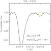 |
Fig. B.1 Coadded spectrum of TOI-1430 around the Li line (solid line). Shaded region represents the line integration for the lithium EW measurement. |
Appendix C Planet TOI-1430 b: results
Figure C.1 shows the corner plot of the posteriors for the main derived parameters of the stellar activity (from the multidimensional GP analysis of Sect. 5) and of the planet TOI-1430 b.
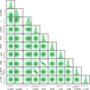 |
Fig. C.1 Corner plot of the posteriors for the main derived parameters of TOI-1430 b and of the stellar activity (multidimensional GP analysis). |
Appendix D Joint Photometric and Spectroscopic analysis of TOI-1430 b through quasiperiodic-GP
We carried out a modelling similar to that described in the Sect. 5, with the exception of using the GP regression, adopting a quasi-periodic kernel as defined by Grunblatt et al. (2015):
![Mathematical equation: $\gamma \left( {{t_i},{t_j}} \right) = H_{{\rm{amp}}}^2\exp \left\{ { - {{{{\sin }^2}\left[ {\pi \left( {{t_i} - {t_j}} \right)/{P_{{\rm{rot}}}}} \right]} \over {2{w^2}}} - {{{{\left( {{t_i} - {t_j}} \right)}^2}} \over {2P_{{\rm{dec}}}^2}}} \right\}$](/articles/aa/full_html/2025/01/aa52236-24/aa52236-24-eq79.png) (D.1)
(D.1)
where Hamp is the amplitude of the signal, and the other parameters are defined in Sect. 5 In this analysis, we treated each dataset with an independent GP regression where only the three main hyper-parameters of the quasi-periodic kernel are shared between the datasets, namely (i) the stellar rotation Prot, (ii) the characteristics decay timescale Pdec, (iii) the coherence scale w. In other words, each dataset is characterized by its own independent covariance matrix, with the activity indicators serving as training datasets for the hyper-parameters. We adopted the same priors used in Sect. 5 and reported, with the results of the model fitting, in Table D.1. Figure D.1 shows the results of the fitting. The most important difference with the multi-GP modeling is that the activity models for different datasets are different; indeed the multidimensional GP regression minimizes the risks of overfitting the activity variations as the underlying GP must be compatible with all the provided radial velocity and activity indicator datasets, even when coming from independent instruments, thus providing more accurate results both inherent in stellar activity and for planetary parameters. Despite the less robust treatment of stellar activity by the quasi-periodic GP, we achieved a comparable precision in the planet RV semi-amplitude compared to the multidimensional GP analysis, with results in agreement well within <1σ, although the median value is slightly higheer (1.6m s−1 versus 1.5 m s−1).
Also in this case we tested the non-null eccentricity case, obtaining  and similar results of Table D.1. Running the dynamic nested sampling algorithm, in the case of circular orbit, we obtained a log 𝒵 ≃ 286.6, while in the case of Keplerian orbit log 𝒵 ≃ 285.0; the circular model is preferred also in this case.
Stellar activity with quasiperiodic GP and orbital parameters of TOI-1430 b
Appendix E The candidate planet c
In addition to the analysis done in Sect. 5.1, we searched for the signal of a second planet modeling the activity with the quasi-periodic GP regression and the same priors reported in Table D.1. We run PyORBIT to search for planetary signals in the range of periods 0.4 ≤ Pc ≤ 100.0 days and RV semi-amplitude 0.01 ≤ Kc ≤ 10.00 m/s. Chains converged after 100000 steps, resulting in a signal with period Pc = 13.27 ± 0.02 d and RV semi-amplitude Kc = 2.5 ± 0.5 m/s (corresponding to a mass MP,csin ic = 8.2 ± 1.7M⊕); the resulting parameters for planet TOI-1430 b are the same reported in Table D.1. Different models give different results (Table E.1, Fig. E.1), leading to the conclusion that the signal of candidate TOI-1430 c is actually due to residual of stellar activity.
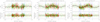 |
Fig. E.1 Candidate planet c signal obtained with different stellar activity models. From the left to the right: activity modelled with multidimensional GP and orbital period boundaries between 0.4 d and 100.0 d (Pc ~ 96.4 d); activity modelled with multidimensional GP and orbital period boundaries between 0.4 d and 20.0 d (Pc ~ 12.7 d); activity modelled with quasi-periodic GP (Pc ~ 13.3 d). |
Orbital parameters of the candidate TOI-1430 c from RV analysis with different activity models
Appendix F TTV Analysis
In Table F.1 the Central times and Planetary-to-stellar-radius ratio from the transits observed with TESS and LCO facilities are reported. Figure F.1 shows the modeling of single transits observed by TESS and LCO.
Central times and Planetary-to-stellar-radius ratio from the transits observed with TESS and LCO facilities
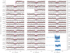 |
Fig. F.1 Analysis of TTVs based on TESS (gray points) and LCO (azure points) data. Panels shows every single transit centred on the expected T0 (magenta dashed line) and the fitted model (in red). Below each transit, the residuals are reported. |
References
- Agol, E., Steffen, J., Sari, R., & Clarkson, W. 2005, MNRAS, 359, 567 [Google Scholar]
- Almeida-Fernandes, F. & Rocha-Pinto, H. J. 2018, MNRAS, 476, 184 [Google Scholar]
- Bailer-Jones, C. A. L., Rybizki, J., Fouesneau, M., Demleitner, M., & Andrae, R. 2021, AJ, 161, 147 [Google Scholar]
- Baliunas, S. L., Donahue, R. A., Soon, W. H., et al. 1995, ApJ, 438, 269 [Google Scholar]
- Baratella, M., D’Orazi, V., Biazzo, K., et al. 2020, A&A, 640, A123 [NASA ADS] [CrossRef] [EDP Sciences] [Google Scholar]
- Barragán, O., Aigrain, S., Rajpaul, V. M., & Zicher, N. 2022a, MNRAS, 509, 866 [Google Scholar]
- Barragán, O., Armstrong, D. J., Gandolfi, D., et al. 2022b, MNRAS, 514, 1606 [CrossRef] [Google Scholar]
- Barragán, O., Gillen, E., Aigrain, S., et al. 2023, MNRAS, 522, 3458 [CrossRef] [Google Scholar]
- Barragán, O., Yu, H., Freckelton, A. V., et al. 2024, MNRAS, 531, 4275 [CrossRef] [Google Scholar]
- Battley, M. P., Armstrong, D. J., & Pollacco, D. 2022, MNRAS, 511, 4285 [NASA ADS] [CrossRef] [Google Scholar]
- Benatti, S., Nardiello, D., Malavolta, L., et al. 2019, A&A, 630, A81 [NASA ADS] [CrossRef] [EDP Sciences] [Google Scholar]
- Benatti, S., Damasso, M., Borsa, F., et al. 2021, A&A, 650, A66 [NASA ADS] [CrossRef] [EDP Sciences] [Google Scholar]
- Biazzo, K., D’Orazi, V., Desidera, S., et al. 2022, A&A, 664, A161 [NASA ADS] [CrossRef] [EDP Sciences] [Google Scholar]
- Bouma, L. G., Hartman, J. D., Bhatti, W., Winn, J. N., & Bakos, G. Á. 2019, ApJS, 245, 13 [Google Scholar]
- Bouma, L. G., Hartman, J. D., Brahm, R., et al. 2020, AJ, 160, 239 [Google Scholar]
- Bressan, A., Marigo, P., Girardi, L., et al. 2012, MNRAS, 427, 127 [NASA ADS] [CrossRef] [Google Scholar]
- Brewer, J. M., Fischer, D. A., Valenti, J. A., & Piskunov, N. 2016, ApJS, 225, 32 [Google Scholar]
- Buchner, J. 2016, Statist. Comput., 26, 383 [NASA ADS] [CrossRef] [Google Scholar]
- Butler, R. P., Marcy, G. W., Williams, E., et al. 1996, PASP, 108, 500 [Google Scholar]
- Caldiroli, A., Haardt, F., Gallo, E., et al. 2021, A&A, 655, A30 [NASA ADS] [CrossRef] [EDP Sciences] [Google Scholar]
- Caldiroli, A., Haardt, F., Gallo, E., et al. 2022, A&A, 663, A122 [NASA ADS] [CrossRef] [EDP Sciences] [Google Scholar]
- Carleo, I., Malavolta, L., Lanza, A. F., et al. 2020, A&A, 638, A5 [NASA ADS] [CrossRef] [EDP Sciences] [Google Scholar]
- Carleo, I., Malavolta, L., Desidera, S., et al. 2024, A&A, 682, A135 [NASA ADS] [CrossRef] [EDP Sciences] [Google Scholar]
- Casagrande, L., Lin, J., Rains, A. D., et al. 2021, MNRAS, 507, 2684 [NASA ADS] [CrossRef] [Google Scholar]
- Castelli, F., & Kurucz, R. L. 2003, in Modelling of Stellar Atmospheres, 210, eds. N. Piskunov, W. W. Weiss, & D. F. Gray, A20 [NASA ADS] [Google Scholar]
- Choi, J., Dotter, A., Conroy, C., et al. 2016, ApJ, 823, 102 [Google Scholar]
- Chontos, A., Murphy, J.M.A., MacDougall, M. G., et al. 2022, AJ, 163, 297 [NASA ADS] [CrossRef] [Google Scholar]
- Claudi, R., Bruno, G., Fossati, L., et al. 2024, A&A, 682, A136 [NASA ADS] [CrossRef] [EDP Sciences] [Google Scholar]
- Cosentino, R., Lovis, C., Pepe, F., et al. 2012, SPIE Conf. Ser., 8446, 84461V [Google Scholar]
- Costes, J. C., Watson, C. A., de Mooij, E., et al. 2021, MNRAS, 505, 830 [NASA ADS] [CrossRef] [Google Scholar]
- Covino, E., Esposito, M., Barbieri, M., et al. 2013, A&A, 554, A28 [NASA ADS] [CrossRef] [EDP Sciences] [Google Scholar]
- Cutri, R. M., Skrutskie, M. F., van Dyk, S., et al. 2003, 2MASS All Sky Catalog of point sources [Google Scholar]
- Dai, F., Roy, A., Fulton, B., et al. 2020, AJ, 160, 193 [NASA ADS] [CrossRef] [Google Scholar]
- Dalba, P. A., Gupta, A. F., Rodriguez, J. E., et al. 2020, AJ, 159, 241 [NASA ADS] [CrossRef] [Google Scholar]
- Damasso, M., Esposito, M., Nascimbeni, V., et al. 2015, A&A, 581, L6 [NASA ADS] [CrossRef] [EDP Sciences] [Google Scholar]
- Damasso, M., Locci, D., Benatti, S., et al. 2023, A&A, 672, A126 [NASA ADS] [CrossRef] [EDP Sciences] [Google Scholar]
- Damasso, M., Polychroni, D., Locci, D., et al. 2024, A&A, 688, A15 [NASA ADS] [CrossRef] [EDP Sciences] [Google Scholar]
- da Silva, L., Girardi, L., Pasquini, L., et al. 2006, A&A, 458, 609 [NASA ADS] [CrossRef] [EDP Sciences] [Google Scholar]
- Desidera, S., Covino, E., Messina, S., et al. 2015, A&A, 573, A126 [NASA ADS] [CrossRef] [EDP Sciences] [Google Scholar]
- Desidera, S., Damasso, M., Gratton, R., et al. 2023, A&A, 675, A158 [NASA ADS] [CrossRef] [EDP Sciences] [Google Scholar]
- Dutra-Ferreira, L., Pasquini, L., Smiljanic, R., Porto de Mello, G. F., & Steffen, M. 2016, A&A, 585, A75 [NASA ADS] [CrossRef] [EDP Sciences] [Google Scholar]
- Eastman, J., Siverd, R., & Gaudi, B. S. 2010, PASP, 122, 935 [Google Scholar]
- Erkaev, N. V., Kulikov, Y. N., Lammer, H., et al. 2007, A&A, 472, 329 [NASA ADS] [CrossRef] [EDP Sciences] [Google Scholar]
- Filomeno, S., Biazzo, K., Baratella, M., et al. 2024, A&A, 690, A370 [NASA ADS] [CrossRef] [EDP Sciences] [Google Scholar]
- Foreman-Mackey, D., Hogg, D. W., Lang, D., & Goodman, J. 2013, PASP, 125, 306 [Google Scholar]
- Fortney, J. J., Marley, M. S., & Barnes, J. W. 2007, ApJ, 659, 1661 [Google Scholar]
- Fulton, B. J., & Petigura, E. A. 2018, AJ, 156, 264 [Google Scholar]
- Fulton, B. J., Petigura, E. A., Howard, A. W., et al. 2017, AJ, 154, 109 [Google Scholar]
- Gaia Collaboration (Smart, R. L., et al.) 2021, A&A, 649, A6 [EDP Sciences] [Google Scholar]
- Gaia Collaboration (Vallenari, A., et al.) 2023, A&A, 674, A1 [NASA ADS] [CrossRef] [EDP Sciences] [Google Scholar]
- Gaidos, E., Hirano, T., Lee, R. A., et al. 2023, MNRAS, 518, 3777 [Google Scholar]
- Giacalone, S., Dressing, C. D., Jensen, E. L. N., et al. 2021, AJ, 161, 24 [Google Scholar]
- Giacalone, S., Dressing, C. D., García Muñoz, A., et al. 2022a, ApJ, 935, L10 [Google Scholar]
- Giacalone, S., Dressing, C. D., Hedges, C., et al. 2022b, AJ, 163, 99 [NASA ADS] [CrossRef] [Google Scholar]
- Ginzburg, S., Schlichting, H. E., & Sari, R. 2018, MNRAS, 476, 759 [Google Scholar]
- Gomes da Silva, J., Figueira, P., Santos, N., & Faria, J. 2018, J. Open Source Softw., 3, 667 [Google Scholar]
- Gomes da Silva, J., Santos, N. C., Adibekyan, V., et al. 2021, A&A, 646, A77 [NASA ADS] [CrossRef] [EDP Sciences] [Google Scholar]
- Goodman, J., & Weare, J. 2010, Commun. Appl. Math. Computat. Sci., 5, 65 [Google Scholar]
- Granata, V., Nascimbeni, V., Piotto, G., et al. 2014, Astron. Nachr., 335, 797 [NASA ADS] [CrossRef] [Google Scholar]
- Grunblatt, S. K., Howard, A. W., & Haywood, R. D. 2015, ApJ, 808, 127 [NASA ADS] [CrossRef] [Google Scholar]
- Guilluy, G., D’Arpa, M. C., Bonomo, A. S., et al. 2024, A&A, 686, A83 [NASA ADS] [CrossRef] [EDP Sciences] [Google Scholar]
- Gupta, A., & Schlichting, H. E. 2019, MNRAS, 487, 24 [Google Scholar]
- Henning, W. G., O’Connell, R. J., & Sasselov, D. D. 2009, ApJ, 707, 1000 [Google Scholar]
- Higson, E., Handley, W., Hobson, M., & Lasenby, A. 2019, Statist. Comput., 29, 891 [Google Scholar]
- Hippke, M., & Heller, R. 2019, A&A, 623, A39 [NASA ADS] [CrossRef] [EDP Sciences] [Google Scholar]
- Hippke, M., David, T. J., Mulders, G. D., & Heller, R. 2019, AJ, 158, 143 [Google Scholar]
- Holman, M. J., & Murray, N. W. 2005, Science, 307, 1288 [Google Scholar]
- Howard, A. W., Johnson, J. A., Marcy, G. W., et al. 2010, ApJ, 721, 1467 [Google Scholar]
- Hünsch, M., Schmitt, J. H. M. M., Sterzik, M. F., & Voges, W. 1999, A&AS, 135, 319 [CrossRef] [EDP Sciences] [Google Scholar]
- Husser, T.-O., Wende-von Berg, S., Dreizler, S., et al. 2013, A&A, 553, A6 [NASA ADS] [CrossRef] [EDP Sciences] [Google Scholar]
- Isaacson, H., Kane, S. R., Carter, B., et al. 2024, ApJ, 961, 85 [NASA ADS] [CrossRef] [Google Scholar]
- Jenkins, J. M., Twicken, J. D., McCauliff, S., et al. 2016, SPIE Conf. Ser., 9913, 99133E [Google Scholar]
- Johnstone, C. P., Bartel, M., & Güdel, M. 2021, A&A, 649, A96 [EDP Sciences] [Google Scholar]
- Kabáth, P., Chaturvedi, P., MacQueen, P. J., et al. 2022, MNRAS, 513, 5955 [CrossRef] [Google Scholar]
- Kervella, P., Arenou, F., & Thévenin, F. 2022, A&A, 657, A7 [NASA ADS] [CrossRef] [EDP Sciences] [Google Scholar]
- Kipping, D. M. 2010, MNRAS, 408, 1758 [Google Scholar]
- Kipping, D. M. 2013, MNRAS, 435, 2152 [Google Scholar]
- Kreidberg, L. 2015, PASP, 127, 1161 [Google Scholar]
- Lampón, M., López-Puertas, M., Lara, L. M., et al. 2020, A&A, 636, A13 [NASA ADS] [CrossRef] [EDP Sciences] [Google Scholar]
- Lange, S., Murphy, J. M. A., Batalha, N. M., et al. 2024, AJ, 167, 282 [Google Scholar]
- Leonardi, P., Nascimbeni, V., Granata, V., et al. 2024, A&A, 686, A84 [NASA ADS] [CrossRef] [EDP Sciences] [Google Scholar]
- Libralato, M., Bedin, L. R., Nardiello, D., & Piotto, G. 2016, MNRAS, 456, 1137 [NASA ADS] [CrossRef] [Google Scholar]
- Lind, K., Asplund, M., & Barklem, P. S. 2009, A&A, 503, 541 [NASA ADS] [CrossRef] [EDP Sciences] [Google Scholar]
- Locci, D., Cecchi-Pestellini, C., & Micela, G. 2019, A&A, 624, A101 [NASA ADS] [CrossRef] [EDP Sciences] [Google Scholar]
- Lopez, E. D., & Fortney, J. J. 2014, ApJ, 792, 1 [Google Scholar]
- Lopez, E. D., Fortney, J. J., & Miller, N. 2012, ApJ, 761, 59 [Google Scholar]
- Lovis, C., Dumusque, X., Santos, N. C., et al. 2011, arXiv e-prints [arXiv:1107.5325] [Google Scholar]
- MacDougall, M. G., Petigura, E. A., Angelo, I., et al. 2021, AJ, 162, 265 [Google Scholar]
- Maggio, A., Locci, D., Pillitteri, I., et al. 2022, ApJ, 925, 172 [NASA ADS] [CrossRef] [Google Scholar]
- Malavolta, L. 2016, Astrophysics Source Code Library [record ascl:1612.008] [Google Scholar]
- Malavolta, L., Nascimbeni, V., Piotto, G., et al. 2016, A&A, 588, A118 [NASA ADS] [CrossRef] [EDP Sciences] [Google Scholar]
- Malavolta, L., Mayo, A. W., Louden, T., et al. 2018, AJ, 155, 107 [NASA ADS] [CrossRef] [Google Scholar]
- Maldonado, J., Colombo, S., Petralia, A., et al. 2022, A&A, 663, A142 [NASA ADS] [CrossRef] [EDP Sciences] [Google Scholar]
- Maldonado, J., Petralia, A., Mantovan, G., et al. 2023, A&A, 674, A132 [NASA ADS] [CrossRef] [EDP Sciences] [Google Scholar]
- Mallonn, M., von Essen, C., Weingrill, J., et al. 2015, A&A, 580, A60 [NASA ADS] [CrossRef] [EDP Sciences] [Google Scholar]
- Mallonn, M., Herrero, E., Juvan, I. G., et al. 2018, A&A, 614, A35 [NASA ADS] [CrossRef] [EDP Sciences] [Google Scholar]
- Mamajek, E. E., & Hillenbrand, L. A. 2008, ApJ, 687, 1264 [Google Scholar]
- Mann, A. W., Johnson, M. C., Vanderburg, A., et al. 2020, AJ, 160, 179 [Google Scholar]
- Mann, A. W., Wood, M. L., Schmidt, S. P., et al. 2022, AJ, 163, 156 [NASA ADS] [CrossRef] [Google Scholar]
- Mantovan, G., Montalto, M., Piotto, G., et al. 2022, MNRAS, 516, 4432 [NASA ADS] [CrossRef] [Google Scholar]
- Mantovan, G., Malavolta, L., Desidera, S., et al. 2024a, A&A, 682, A129 [NASA ADS] [CrossRef] [EDP Sciences] [Google Scholar]
- Mantovan, G., Malavolta, L., Locci, D., et al. 2024b, A&A, 684, L17 [NASA ADS] [CrossRef] [EDP Sciences] [Google Scholar]
- Masson, A., Vinatier, S., Bézard, B., et al. 2024, A&A, 688, A179 [NASA ADS] [CrossRef] [EDP Sciences] [Google Scholar]
- McCully, C., Turner, M., Volgenau, N., et al. 2018, https://doi.org/10.5281/zenodo.1257560 [Google Scholar]
- Montalto, M., Piotto, G., Marrese, P. M., et al. 2021, A&A, 653, A98 [NASA ADS] [CrossRef] [EDP Sciences] [Google Scholar]
- Montes, D., López-Santiago, J., Gálvez, M. C., et al. 2001, MNRAS, 328, 45 [NASA ADS] [CrossRef] [Google Scholar]
- Nardiello, D. 2020, MNRAS, 498, 5972 [Google Scholar]
- Nardiello, D., Bedin, L. R., Nascimbeni, V., et al. 2015, MNRAS, 447, 3536 [CrossRef] [Google Scholar]
- Nardiello, D., Libralato, M., Bedin, L. R., et al. 2016a, MNRAS, 463, 1831 [NASA ADS] [CrossRef] [Google Scholar]
- Nardiello, D., Libralato, M., Bedin, L. R., et al. 2016b, MNRAS, 455, 2337 [NASA ADS] [CrossRef] [Google Scholar]
- Nardiello, D., Borsato, L., Piotto, G., et al. 2019, MNRAS, 490, 3806 [NASA ADS] [CrossRef] [Google Scholar]
- Nardiello, D., Piotto, G., Deleuil, M., et al. 2020, MNRAS, 495, 4924 [Google Scholar]
- Nardiello, D., Deleuil, M., Mantovan, G., et al. 2021, MNRAS, 505, 3767 [NASA ADS] [CrossRef] [Google Scholar]
- Nardiello, D., Malavolta, L., Desidera, S., et al. 2022, A&A, 664, A163 [NASA ADS] [CrossRef] [EDP Sciences] [Google Scholar]
- Nascimbeni, V., Piotto, G., Bedin, L. R., & Damasso, M. 2011a, A&A, 527, A85 [NASA ADS] [CrossRef] [EDP Sciences] [Google Scholar]
- Nascimbeni, V., Piotto, G., Bedin, L. R., et al. 2011b, A&A, 532, A24 [NASA ADS] [CrossRef] [EDP Sciences] [Google Scholar]
- Nascimbeni, V., Cunial, A., Murabito, S., et al. 2013, A&A, 549, A30 [NASA ADS] [CrossRef] [EDP Sciences] [Google Scholar]
- Newton, E. R., Mann, A. W., Tofflemire, B. M., et al. 2019, ApJ, 880, L17 [Google Scholar]
- Newton, E. R., Mann, A. W., Kraus, A. L., et al. 2021, AJ, 161, 65 [NASA ADS] [CrossRef] [Google Scholar]
- Oelkers, R. J., Rodriguez, J. E., Stassun, K. G., et al. 2018, AJ, 155, 39 [Google Scholar]
- Oh, S., Price-Whelan, A. M., Hogg, D. W., Morton, T. D., & Spergel, D. N. 2017, AJ, 153, 257 [NASA ADS] [CrossRef] [Google Scholar]
- Orell-Miquel, J., Lampón, M., López-Puertas, M., et al. 2023, A&A, 677, A56 [NASA ADS] [CrossRef] [EDP Sciences] [Google Scholar]
- Owen, J. E., & Wu, Y. 2013, ApJ, 775, 105 [Google Scholar]
- Owen, J. E., & Wu, Y. 2017, ApJ, 847, 29 [Google Scholar]
- Parviainen, H., & Aigrain, S. 2015, MNRAS, 453, 3821 [Google Scholar]
- Pecaut, M. J., & Mamajek, E. E. 2013, ApJS, 208, 9 [Google Scholar]
- Penz, T., Micela, G., & Lammer, H. 2008, A&A, 477, 309 [NASA ADS] [CrossRef] [EDP Sciences] [Google Scholar]
- Pepe, F., Mayor, M., Galland, F., et al. 2002, A&A, 388, 632 [NASA ADS] [CrossRef] [EDP Sciences] [Google Scholar]
- Pepper, J., Pogge, R. W., DePoy, D. L., et al. 2007, PASP, 119, 923 [NASA ADS] [CrossRef] [Google Scholar]
- Pérez-González, J., Greklek-McKeon, M., Vissapragada, S., et al. 2024, AJ, 167, 214 [CrossRef] [Google Scholar]
- Pino, L., Brogi, M., Désert, J. M., et al. 2022, A&A, 668, A176 [NASA ADS] [CrossRef] [EDP Sciences] [Google Scholar]
- Pizzolato, N., Maggio, A., Micela, G., Sciortino, S., & Ventura, P. 2003, A&A, 397, 147 [NASA ADS] [CrossRef] [EDP Sciences] [Google Scholar]
- Polanski, A. S., Lubin, J., Beard, C., et al. 2024, ApJS, 272, 32 [NASA ADS] [CrossRef] [Google Scholar]
- Queloz, D., Eggenberger, A., Mayor, M., et al. 2000, A&A, 359, L13 [NASA ADS] [Google Scholar]
- Rajpaul, V., Aigrain, S., Osborne, M. A., Reece, S., & Roberts, S. 2015, MNRAS, 452, 2269 [Google Scholar]
- Ricker, G. R., Winn, J. N., Vanderspek, R., et al. 2015, J. Astron. Telesc. Instrum. Syst., 1, 014003 [Google Scholar]
- Rizzuto, A. C., Newton, E. R., Mann, A. W., et al. 2020, AJ, 160, 33 [Google Scholar]
- Sanz-Forcada, J., López-Puertas, M., Nortmann, L., & Lampón, M. 2022, 21st Cambridge Workshop on Cool Stars, Stellar Systems, and the Sun, https://backoffice.inviteo.com/upload/compte153/Base/inscriptions_projets/fichier/108345-posterjsanzcs21.pdf [Google Scholar]
- Shi, X.-d., Qian, S.-b., & Li, L.-J. 2022, ApJS, 259, 50 [NASA ADS] [CrossRef] [Google Scholar]
- Sicilia, D., Scandariato, G., Guilluy, G., et al. 2024, A&A, 687, A143 [NASA ADS] [CrossRef] [EDP Sciences] [Google Scholar]
- Skrutskie, M. F., Cutri, R. M., Stiening, R., et al. 2006, AJ, 131, 1163 [NASA ADS] [CrossRef] [Google Scholar]
- Smith, J. C., Stumpe, M. C., Van Cleve, J. E., et al. 2012, PASP, 124, 1000 [Google Scholar]
- Sneden, C. 1973, ApJ, 184, 839 [Google Scholar]
- Soubiran, C., Jasniewicz, G., Chemin, L., et al. 2018, A&A, 616, A7 [NASA ADS] [CrossRef] [EDP Sciences] [Google Scholar]
- Sousa, S. G., Santos, N. C., Adibekyan, V., Delgado-Mena, E., & Israelian, G. 2015, A&A, 577, A67 [NASA ADS] [CrossRef] [EDP Sciences] [Google Scholar]
- Speagle, J. S. 2020, MNRAS, 493, 3132 [Google Scholar]
- Spinelli, R., Gallo, E., Haardt, F., et al. 2023, AJ, 165, 200 [NASA ADS] [CrossRef] [Google Scholar]
- Stassun, K. G., Oelkers, R. J., Pepper, J., et al. 2018, AJ, 156, 102 [Google Scholar]
- Stassun, K. G., Oelkers, R. J., Paegert, M., et al. 2019, AJ, 158, 138 [Google Scholar]
- Storn, R., & Price, K. 1997, J. Global Optim., 11, 341 [Google Scholar]
- Strassmeier, K. G., Granzer, T., Weber, M., et al. 2004, Astron. Nachr., 325, 527 [NASA ADS] [CrossRef] [Google Scholar]
- Stumpe, M. C., Smith, J. C., Van Cleve, J. E., et al. 2012, PASP, 124, 985 [Google Scholar]
- Stumpe, M. C., Smith, J. C., Catanzarite, J. H., et al. 2014, PASP, 126, 100 [Google Scholar]
- Thao, P. C., Mann, A. W., Barber, M. G., et al. 2024, AJ, 168, 41 [Google Scholar]
- Tofflemire, B. M., Rizzuto, A. C., Newton, E. R., et al. 2021, AJ, 161, 171 [NASA ADS] [CrossRef] [Google Scholar]
- Vach, S., Quinn, S. N., Vanderburg, A., et al. 2022, AJ, 164, 71 [NASA ADS] [CrossRef] [Google Scholar]
- Voges, W., Aschenbach, B., Boller, T., et al. 2000, IAU Circ., 7432, 3 [NASA ADS] [Google Scholar]
- Vogt, S. S., Allen, S. L., Bigelow, B. C., et al. 1994, SPIE Conf. Ser., 2198, 362 [NASA ADS] [Google Scholar]
- Vogt, S. S., Radovan, M., Kibrick, R., et al. 2014, PASP, 126, 359 [NASA ADS] [CrossRef] [Google Scholar]
- Winn, J. N. 2010, in Exoplanets, ed. S. Seager, 55 [Google Scholar]
- Wood, M. L., Mann, A. W., Barber, M. G., et al. 2023, AJ, 165, 85 [NASA ADS] [CrossRef] [Google Scholar]
- Wright, E. L., Eisenhardt, P. R. M., Mainzer, A. K., et al. 2010, AJ, 140, 1868 [Google Scholar]
- Wright, N. J., Drake, J. J., Mamajek, E. E., & Henry, G. W. 2011, ApJ, 743, 48 [Google Scholar]
- Wright, N. J., Newton, E. R., Williams, P. K. G., Drake, J. J., & Yadav, R. K. 2018, MNRAS, 479, 2351 [Google Scholar]
- Xu, C., McCully, C., Dong, B., Howell, D. A., & Sen, P. 2023, ApJ, 942, 73 [Google Scholar]
- Zechmeister, M., & Kürster, M. 2009, A&A, 496, 577 [CrossRef] [EDP Sciences] [Google Scholar]
- Zeng, L., Jacobsen, S. B., Sasselov, D. D., et al. 2019, PNAS, 116, 9723 [Google Scholar]
- Zhang, M., Knutson, H. A., Dai, F., et al. 2023, AJ, 165, 62 [NASA ADS] [CrossRef] [Google Scholar]
Although the K2 mask would be the best choice for this star, it is currently not available in the YABI interface. However, we do not expect this choice to affect the RV precision, which is limited by stellar activity.
Our slightly larger uncertainty is based on a conservative choice considering the variability due to the prominent activity cycle and the possible effects on the stellar inclination.
Updated values at: https://www.pas.rochester.edu/~emamajek/EEM_dwarf_UBVIJHK_colors_Teff.txt
In this work we used NVIDIA RTX A5500 GPU.
All Tables
Orbital parameters of the candidate TOI-1430 c from RV analysis with different activity models
Central times and Planetary-to-stellar-radius ratio from the transits observed with TESS and LCO facilities
All Figures
|
Fig. 1 Finding chart (15 × 15 arcmin2) of TOI-1430 (cyan diamond) from a TESS Full Frame Image. Neighboring stars with G ≤ 15 are identified with red circles, the radii of which are inversely proportional to the difference between the magnitude of TOI-1430 and that of its neighbors. The green circle indicates the eclipsing binary that generates the spurious signal in the SAP light curves. |
| In the text | |
|
Fig. 2 Light curves of TOI-1430 obtained with different instruments. From top to bottom: TESS light curve (black dots) obtained from shortcadence data of sectors 14, 15, 16, 41, 54, 55, 56, 75, and 76, KELT light curve (blue crosses), STELLA light curves (green and red squares for V and I bands, respectively), Asiago Schmidt 67/92 cm u-sloan light curve (magenta squares), and LCO light curves in zs filter (azure circles). Vertical dashed lines in the upper panel indicate the gaps between the different years of the TESS mission. |
| In the text | |
|
Fig. 3 Spectroscopic time series obtained with HARPS-N (green squares), HIRES (red circles), and APF (blue triangles) and used in this work. From the top to bottom panels: The RV, the log R′HK, the Hα, and the BIS time series. Dashed orange lines represent the fifth-degree polynomial models used for the modeling of the long trend in the spectroscopic series. The RVs have been reported in the same scale by applying an offset to them; the log R′HK series are calibrated in the same Mt. Wilson scale (Baliunas et al. 1995). |
| In the text | |
|
Fig. 4 Analysis of the rotation period of TOI-1430 performed with different photometric series. The left panels show the light curves folded with the period associated with the peak of the corresponding GLS periodogram (right panels). Φ is the rotational phase of the star. From the upper panel to the bottom, we report the analysis carried out on TESS, KELT, STELLA, and Asiago Schmidt light curves, respectively. |
| In the text | |
|
Fig. 5 Analysis of the rotation period of TOI-1430 carried out on the HARPS-N (five upper panels) and HIRES (three bottom panels) spectroscopic series shown in Fig. 3 (after the subtraction of the long trend). Panels show the GLS periodograms extracted from the RV, log |
| In the text | |
|
Fig. 6 Detection and vetting of the candidate exoplanet TOI-1430.01. Panel a shows the stacked light curve of TOI-1430 and the detrending model (in red). Panel b shows the flattened light curve and the position of the odd (magenta) and even (blue) transits. Panels c are a comparison between the mean depths of the odd and even transits; the dashed lines are the mean depths while the shaded colored regions represent the 3σ confidence interval. Panel d is the TLS periodogram: the period of the peak is indicated with a green triangle. |
| In the text | |
|
Fig. 7 In-/out-of-transit centroid analysis for TOI-1430.01. TOI-1430 is centered on (0,0). Black filled circles are the neighboring stars from Gaia DR3; the dimensions of the points are proportional to the apparent luminosity of the stars. Each colored point corresponds to the average of the centroids in each sector. Within the errors, centroids match with the position of TOI-1430. |
| In the text | |
|
Fig. 8 Overview of the modeling that uses the multidimensional GP for the stellar activity. From the top, the first four panels show the RV, log |
| In the text | |
|
Fig. 9 Analysis of TTVs based on TESS and LCO data. The figure shows the O–C plot of the observed (O) and calculated (C) transit times for the linear ephemeris of TOI-1430 b. |
| In the text | |
|
Fig. 10 Mass–radius diagram for young (<1 Gyr) planets with precise age estimates (relative errors <50%). TOI- 1430 b is located at the edge of the Fulton gap; the arrow indicates the final position in the diagram in the next 200 Myr, when it will completely lose its atmosphere. The Zeng et al. (2019) tracks are reported in magenta (dot-dashed lines) in the case of planets composed of 100% Fe, 32.5% Fe+67.5% MgSiO3 (Earthlike), 50% Earth+50% H2O, and 99.7% Earth+0.3% H2; the Lopez & Fortney (2014) tracks for exoplanets with H/He envelopes between 0.01% and 1% are reported in green. Exoplanets with accurate age estimation are color-coded on the basis of the color bar at the top of the figure; square points are the exoplanets with accurate mass measurement, and triangles are the exoplanets with a mass upper limit measurement. |
| In the text | |
|
Fig. 11 Evolutionary track of TOI 1430 in the effective temperature- bolometric luminosity plane. A gray dot marks the current location of the star on the track. |
| In the text | |
|
Fig. 12 Time evolution of X-ray (5–100 Å), EUV (100–920 Å), and total XUV luminosity of TOI 1430, according to Penz et al. (2008) and the X-ray/EUV scaling by Sanz-Forcada et al. (2022) (red lines) and according to Johnstone et al. (2021) (blue lines). Uncertainties on the age and X-ray luminosity of TOI 1430 are also indicated. The gray area is the original locus for dG stars in Penz et al. (2008). |
| In the text | |
|
Fig. 13 Evolution of the planetary mass (upper-left panel), planetary radius (upper-right panel), atmospheric mass-loss rate (bottom-left panel), and atmospheric mass fraction (bottom-right panel) according to our models with different assumptions. Black squares mark the current location of the star in each plot. |
| In the text | |
|
Fig. A.1 Comparison between the PATHOS and official TESS light curves of TOI-1430. Panel (a) shows the SAP and the PDCSAP light curves (in magenta and blue, respectively) compared to the PATHOS raw and corrected light curves (in red and green, respectively). Gray dashed vertical lines separate the different years in which TOI-1430 was observed by TESSṖanel (b) shows a zoom-in of the raw PATHOS (red) and SAP (magenta) light curves at BTJD= 2790 ± 2 d: spurious signals are detectable at BTJD~eq2788.7 and BTJD~eq2791.5 Panel (c) shows the detrended raw PATHOS and SAP light curves phased with a period P= 2.8137 d, and demonstrates that the systematic signal at 2.8137 d is not present in the PATHOS light curve. |
| In the text | |
|
Fig. B.1 Coadded spectrum of TOI-1430 around the Li line (solid line). Shaded region represents the line integration for the lithium EW measurement. |
| In the text | |
|
Fig. C.1 Corner plot of the posteriors for the main derived parameters of TOI-1430 b and of the stellar activity (multidimensional GP analysis). |
| In the text | |
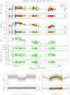 |
Fig. D.1 As Fig. 8, by adopting the quasi-periodic GP regression for the stellar activity. |
| In the text | |
|
Fig. E.1 Candidate planet c signal obtained with different stellar activity models. From the left to the right: activity modelled with multidimensional GP and orbital period boundaries between 0.4 d and 100.0 d (Pc ~ 96.4 d); activity modelled with multidimensional GP and orbital period boundaries between 0.4 d and 20.0 d (Pc ~ 12.7 d); activity modelled with quasi-periodic GP (Pc ~ 13.3 d). |
| In the text | |
|
Fig. F.1 Analysis of TTVs based on TESS (gray points) and LCO (azure points) data. Panels shows every single transit centred on the expected T0 (magenta dashed line) and the fitted model (in red). Below each transit, the residuals are reported. |
| In the text | |
Current usage metrics show cumulative count of Article Views (full-text article views including HTML views, PDF and ePub downloads, according to the available data) and Abstracts Views on Vision4Press platform.
Data correspond to usage on the plateform after 2015. The current usage metrics is available 48-96 hours after online publication and is updated daily on week days.
Initial download of the metrics may take a while.