| Issue |
A&A
Volume 682, February 2024
|
|
|---|---|---|
| Article Number | A135 | |
| Number of page(s) | 18 | |
| Section | Planets and planetary systems | |
| DOI | https://doi.org/10.1051/0004-6361/202348207 | |
| Published online | 14 February 2024 | |
The GAPS programme at TNG
L. TOI-4515 b: An eccentric warm Jupiter orbiting a 1.2 Gyr-old G-star★
1
Instituto de Astrofísica de Canarias (IAC),
Calle Vía Láctea s/n,
38200
La Laguna,
Tenerife,
Spain
e-mail: This email address is being protected from spambots. You need JavaScript enabled to view it.
2
Departamento de Astrofísica, Universidad de La Laguna (ULL),
38206
La Laguna,
Tenerife,
Spain
3
INAF – Osservatorio Astrofisico di Torino,
Via Osservatorio 20,
10025
Pino Torinese,
Italy
4
Dipartimento di Fisica e Astronomia “Galileo Galilei”, Università di Padova,
Vicolo dellOsservatorio 3,
35122
Padova,
Italy
5
INAF – Osservatorio Astronomico di Padova,
Vicolo dell’Osservatorio 5,
35122
Padova,
Italy
6
Astronomy Department, Indiana University,
Bloomington,
IN
47405-7105,
USA
7
INAF – Osservatorio Astrofisico di Catania,
Via S. Sofia 78,
95123
Catania,
Italy
8
Leibniz-Institut für Astrophysik Potsdam (AIP),
An der Sternwarte 16,
14482
Potsdam,
Germany
9
INAF – Osservatorio Astronomico di Palermo,
Piazza del Parlamento 1,
90134
Palermo,
Italy
10
Center for Astrophysics – Harvard & Smithsonian,
60 Garden Street,
Cambridge,
MA
02138,
USA
11
Facultad de Ingeniera y Ciencias, Universidad Adolfo Ibáñez,
Av. Diagonal las Torres 2640,
Peñalolén,
Santiago,
Chile
12
Millennium Institute for Astrophysics,
Monseñor Sotero Sanz 100, of 10,
Providencia,
7500011,
Santiago,
Chile
13
Data Observatory Foundation,
DO, Diagonal Las Torres N. 2460, Building E,
Peñalokén,
Santiago,
Chile
14
SUPA, Institute for Astronomy, University of Edinburgh,
Blackford Hill,
Edinburgh
EH9 3HJ,
UK
15
Astrophysics Group, Keele University,
Staffs
ST5 5BG,
UK
16
Max-Planck-Institut für Astronomie,
Königstuhl 17,
69117
Heidelberg,
Germany
17
Center for Data Intensive and Time Domain Astronomy, Department of Physics and Astronomy, Michigan State University,
East Lansing,
MI
48824,
USA
18
Department of Physics & Astronomy, Vanderbilt University,
Nashville,
TN,
USA
19
Department of Physics, Engineering and Astronomy, Stephen F. Austin State University,
1936 North St,
Nacogdoches,
TX
75962,
USA
20
Fundación Galileo Galilei-INAF,
Rambla José Ana Fernandez Pérez 7,
38712
Breña Baja,
TF,
Spain
21
INAF – Osservatorio Astronomico di Roma,
Via Frascati 33,
00078
Monte Porzio Catone,
Italy
22
Astrobiology Research Unit, Université de Liège,
19C Allée du Six-Août,
4000
Liège,
Belgium
23
Department of Earth, Atmospheric and Planetary Science, Massachusetts Institute of Technology,
77 Massachusetts Avenue,
Cambridge,
MA
02139,
USA
24
INAF – Osservatorio Astronomico di Trieste,
via Tiepolo 11,
34143
Trieste,
Italy
25
INAF – Osservatorio Astronomico di Brera,
Via E. Bianchi 46,
23807
Merate,
Italy
26
Cerro Tololo Inter-American Observatory/NSF’s NOIRLab,
Casilla 603,
La Serena,
Chile
27
Dipartimento di Fisica, Università degli Studi di Torino,
via Pietro Giuria 1,
10125,
Torino,
Italy
28
Dipartimento di Fisica, Sapienza, Università di Roma,
P.le Aldo Moro, 5,
00185
Rome,
Italy
29
NASA Goddard Space Flight Center, Exoplanets and Stellar Astrophysics Laboratory (Code 667),
Greenbelt,
MD
20771,
USA
30
Department of Physics and Astronomy, University of New Mexico,
210 Yale Blvd NE,
Albuquerque,
NM,
USA
31
Department of Physics and Kavli Institute for Astrophysics and Space Research, Massachusetts Institute of Technology,
Cambridge,
MA
02139,
USA
32
Observatori de Ca l’Ou,
Carrer de dalt 18, Sant Martí Sesgueioles
08282,
Barcelona,
Spain
33
Department of Astronomy & Astrophysics, 525 Davey Laboratory, The Pennsylvania State University,
University Park,
PA,
16802,
USA
34
Center for Exoplanets and Habitable Worlds, 525 Davey Laboratory, The Pennsylvania State University,
University Park,
PA
16802,
USA
35
NASA Ames Research Center,
Moffett Field,
CA
94035
USA
36
Department of Physics and Astronomy, The University of North Carolina at Chapel Hill,
Chapel Hill,
NC
27599-3255,
USA
37
NASA Exoplanet Science Institute, IPAC, California Institute of Technology,
Pasadena,
CA
91125,
USA
38
Department of Aeronautics and Astronautics, MIT,
77 Massachusetts Avenue,
Cambridge,
MA
02139,
USA
39
Department of Astrophysical Sciences, Princeton University,
Princeton,
NJ
08544,
USA
40
SETI Institute,
339 N Bernardo Ave Suite 200,
Mountain View,
CA
94043,
USA
Received:
9
October
2023
Accepted:
13
November
2023
Abstract
Context. Different theories have been developed to explain the origins and properties of close-in giant planets, but none of them alone can explain all of the properties of the warm Jupiters (WJs, Porb = 10–200 days). One of the most intriguing characteristics of WJs is that they have a wide range of orbital eccentricities, challenging our understanding of their formation and evolution.
Aims. The investigation of these systems is crucial in order to put constraints on formation and evolution theories. TESS is providing a significant sample of transiting WJs around stars bright enough to allow spectroscopic follow-up studies.
Methods. We carried out a radial velocity (RV) follow-up study of the TESS candidate TOI-4515 b with the high-resolution spectrograph HARPS-N in the context of the GAPS project, the aim of which is to characterize young giant planets, and the TRES and FEROS spectrographs. We then performed a joint analysis of the HARPS-N, TRES, FEROS, and TESS data in order to fully characterize this planetary system.
Results. We find that TOI-4515 b orbits a 1.2 Gyr-old G-star, has an orbital period of Pb = 15.266446 ± 0.000013 days, a mass of Mb = 2.01 ± 0.05 MJ, and a radius of Rb = 1.09 ± 0.04 RJ. We also find an eccentricity of e = 0.46 ± 0.01, placing this planet among the WJs with highly eccentric orbits. As no additional companion has been detected, this high eccentricity might be the consequence of past violent scattering events.
Key words: methods: observational / techniques: photometric / techniques: radial velocities / planets and satellites: detection / planets and satellites: gaseous planets / stars: fundamental parameters
Based on observations made with the Italian Telescopio Nazionale Galileo (TNG) operated by the Fundación Galileo Galilei (FGG) of the Istituto Nazionale di Astrofisica (INAF) at the Observatorio del Roque de los Muchachos (La Palma, Canary Islands, Spain).
© The Authors 2024
 Open Access article, published by EDP Sciences, under the terms of the Creative Commons Attribution License (https://creativecommons.org/licenses/by/4.0), which permits unrestricted use, distribution, and reproduction in any medium, provided the original work is properly cited.
This article is published in open access under the Subscribe to Open model. This email address is being protected from spambots. You need JavaScript enabled to view it. to support open access publication.
1 Introduction
Warm Jupiters (WJs) are gas giant exoplanets with orbital periods of between 10 and 200 days (e.g., Dawson & Johnson 2018), which make them challenging targets for transit detection and radial velocity (RV) follow-up studies compared to their shorter-orbit counterparts (hot Jupiters, HJs). It is for this reason that WJs have so far received less attention. However, these objects are very interesting targets for investigation in order to put constraints on and improve planetary migration theories. Indeed, the observed WJs present a wide span of values in planetary properties, especially in eccentricity (Dong et al. 2021a). They have been detected in low- to moderate-eccentricity orbits (e ≲ 0.4; e.g., Brahm et al. 2016; Niedzielski et al. 2016; Smith et al. 2017), as well as in highly eccentric orbits (e.g., Dawson et al. 2012; Ortiz et al. 2015; Gupta et al. 2023; Dong et al. 2021b). This makes it difficult to link them to a single origin or migration channel; instead, it is thought that the WJ region (around 0.1–1 AU) can be populated by different formation mechanisms (Fig. 1 from Dawson & Johnson 2018). However, very recently, Rodriguez et al. (2023) showed that a wide range of eccentricities are also present in the HJ regime, for orbital periods longer than 5 days, where tidal forces are not strong. This might suggest that the WJ regime and the longer-period HJ regime are connected.
One explanation of the variable eccentricities of WJs is linked to the possible dynamical coupling with a companion in the system (Petrovich & Tremaine 2016). For example, Dong et al. (2014) showed that known WJs with high eccentricities (e ≳ 0.4) or stellar companion in a long-period orbit (see their Fig. 4). The architectures of these systems suggest that eccentric WJs might have undergone high-eccentricity migration excited by the outer companion. Furthermore, Dawson et al. (2012) and Ortiz et al. (2015) present highly eccentric WJs together with the presence of outer companions. However, there are certainly eccentric WJs without detected massive companions (e.g. Schlecker et al. 2020). On the other hand, WJs with no detected giant companion tend to have lower but still significant eccentricities that peak around 0.2 (Dong et al. 2014). However, the mechanisms used to explain the eccentricities have an impact on the stellar obliquity as well. High eccentricities might be correlated to high obliquities (e.g., Dong et al. 2023) and cool stars orbited by distant giant planets like WJs present high obliquities (Albrecht et al. 2022). Discovering and studying these systems in detail is important in order to increase the statistics and better relate the observed properties to theory.
In this paper, we present the discovery of an eccentric WJ, TOI-4515b (TYC 1203-1161-1), which has no known outer companion. The target was selected for the program GAPS-Young Objects (GAPS-YO; Carleo et al. 2020, 2021; Nardiello et al. 2022), the aim of which is to validate, confirm, and determine the mass of transiting planets around young stars (≲700Myr). GAPS-YO is an ongoing program at the Telescopio Nazionale Galileo (TNG) using the HARPS-N spectrograph in the framework of the GAPS program (Covino et al. 2013). A clear photometric modulation is seen in TESS data, suggesting a moderately young age (a few hundred million years). The subsequent analysis presented in this paper indicates that the star is likely slightly older than 1 Gyr, and is therefore more mature than the other targets considered in the GAPS-YO program. Nevertheless, we decided to complete the RV monitoring in order to determine the mass of the WJ, considering the importance of investigating these systems, both by increasing the number of this population and by fully characterizing them.
The paper is organized as follows. The observations and available data are presented in Sect. 2; our analysis aimed at retrieving the stellar properties is described in Sect. 3. The planet validation is presented in Sect. 4, and the joint fit with the retrieved planetary system parameters is presented in Sect. 5. We then present a discussion in Sect. 7 and draw conclusions in Sect. 8.
2 Observations and data reduction
2.1 Photometric data
2.1.1 TESS
TOI-4515 was observed in both short (120s) and long (1800s) cadence by TESS in Sectors 17 (from UT 2019 October 7 to November 2, only in long cadence mode), 42, 43 (from UT 2021 August 20 to 2021 October 12, program IDs: GO-4195, GO-4231, GO-4191), and 57 (UT 2022 September 30 to October 29, GO-5054). The Science Processing Operations Center (SPOC) conducted a transit search of Sector 42 on UT 2021 September 22 with an adaptive, noise-compensating matched filter (Jenkins 2002; Jenkins et al. 2010, 2020), producing a TCE for which an initial limb-darkened transit model was fitted (Li et al. 2019) and a suite of diagnostic tests were conducted to help make or break the planetary nature of the signal (Twicken et al. 2018). The transit signature was also detected in a search of full-frame image (FFI) data by the Quick Look Pipeline (QLP) at Massachusetts Institute of Technology (MIT; Huang et al. 2020a,b). The TESS Science Office (TSO) reviewed the vetting information and issued an alert on UT 2021 October 21 (Guerrero et al. 2021). The signal was repeatedly recovered as additional observations were made in sectors 42, 43, and 57, and the transit signature passed all the diagnostic tests presented in the Data Validation reports on UT 2023 February 6. The host star is located within 0.61 ± 2.53 arcsec of the source of the transit signal.
In this work, we adopted both the short- and long-cadence light curves in order to validate the transits, study the stellar activity, and extract planetary information. Long-cadence light curves are extracted and corrected using the PATHOS pipeline described in detail in Nardiello et al. (2019,2020,2021); Nardiello (2020). For our analysis, we cleaned the light curves excluding all the points flagged with DQUALITY>0. For the short-cadence light curves, we adopted the Presearch Data Conditioning Simple Aperture Photometry (PDCSAP) light curves (Smith et al. 2012; Stumpe et al. 2012, 2014).
In order to verify that no additional sources could contaminate the TESS flux of TOI-4515, we inspected the Target Pixel Files (TPF), which contain the original CCD pixel observations. The code overplots – on the TPF image – all the sources present in the Data Release 3 of Gaia with a specific contrast magnitude with respect to our target (in this case we set ∆m = 8), and highlights the aperture mask employed by the TESS pipeline to measure the SAP flux. According to Fig. 1, only one potentially contaminating source is included within the aperture mask (Gaia DR3 ID 289464440515394944), and has a G-mag equal to 19.67 (∆m ~ 7.9). We note that the crowding reported for each sector in which TOI-4515 is observed is always less than 1% (based on an analysis of the TIC-8 catalog and the pixel response functions reconstructed from dithered data sets obtained at the beginning of the mission). This level of contamination is properly corrected in the PDCSAP curve by the SPOC pipeline. In accordance with the approach outlined in Mantovan et al. (2022), we used Gaia DR3 data to detect nearby contaminating stars that might be blended eclipsing binaries (BEBs) and measure the dilution factor, which denotes the total flux from contaminant stars that fall into the photometric aperture divided by the flux contribution of the target star. Our analysis reveals that, besides TOI-4515, none of the Gaia resolved stars within a radius of ten TESS pixels from the target star can reproduce the transit signal of TOI-4515.01. Additionally, our investigation indicates an almost negligible dilution factor of 0.01.
2.1.2 WASP archival data
The field of TOI-4515 was observed by the WASP transit-search survey (Pollacco et al. 2006) between 2004 and 2014, accumulating a total of 90 000 photometric data points in a broad, visual passband. Observations on each clear night spanned up to 150 days in each year, observing the field with a ~15 min cadence. TOI-4515 is the only bright star within the 48 arc-sec photometric extraction aperture. Looking at the WASP data, we find two possible transit features that match up with the ephemeris in Sect. 3. While these might be real pre-detections of the transit, this is not certain.
2.1.3 KeplerCam
We observed a full transit of TOI-4515.01 on UT 2021 October 25 from KeplerCam on the 1.2 m telescope at the Fred Lawrence Whipple Observatory using a Sloan i′ band filter. The 4096 × 4096 Fairchild CCD 486 detector has an image scale of  per 2 × 2 binned pixel, resulting in a
  field of view. The image data were calibrated and photometric data were extracted using AstroImageJ (Collins et al. 2017). We used circular photometric apertures with radius 4″ centered on TOI-4515. The target star aperture excluded flux from the nearest known neighbor in the Gaia DR3 and TICv8 catalogs (TIC 620491915), which is ~14″ north of TOI-4515. The target star light curve was linearly detrended using the full width at half maximum (FWHM) of the target star point spread function in each image. A clear transit-like event was detected and the light curve included in the global model described in Sect. 5.
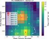 |
Fig. 1 TESS TPF of Sector 17 for TOI-4515. The color bar indicates the electron counts for each pixel. The orange squares show the pixels selected to obtain the aperture photometry by the TESS pipeline. All the sources in Gaia DR3 are overplotted and represented with circles of different sizes according to the G-mag difference with respect to our target (see the legend); this was done with the tpfplotter code (Aller et al. 2020). Gray arrows indicate the direction of the proper motions for all the sources in the plot. |
2.1.4 CALOU
TOI-4515.01 was first released as a TESS Object of Interest from a Sector 42 SPOC Data Validation Report. While the period was released as ~15.265 days, a TESS data gap that occurred due to the spacecraft data download phase of operation allowed a potential planet candidate orbital period alias of 7.6325 days if an additional transit occurred during the data gap. We therefore observed a predicted full transit window – assuming the 7.6325 day period – to check for a transit-like event on an epoch that corresponds to the TESS data gap. We observed the would-be transit window using the Observatori de Ca l’Ou (CALOU), a private observatory in Sant Martí Sesgueioles, near Barcelona Spain, in the Rc passband on UT 2022 January 1. The 0.4 m telescope is equipped with a 1024 × 1024 pixel FLIPL1001 camera with an image scale of  pixel−1, resulting in a 21′ × 21′ field of view. The images were calibrated and differential photometric data were extracted using AstroImageJ. We used a circular photometric aperture with a radius of 10″ centered on TOI-4515 and ruled out the expected ~16 ppt deep event, confirming the true period to be ~15.265 days.
2.1.5 LCOGT
We observed a full transit window (at the ~15.265 days ephemeris) of TOI-4515.01 on 2022 November 11 in Sloan 𝑔′ band using the Las Cumbres Observatory Global Telescope (LCOGT; Brown et al. 2013) 0.4 m network node at Cerro Tololo Inter-American Observatory (CTIO). The 0.4m telescopes are equipped with 2048 × 3072 pixel SBIG STX6303 cameras with an image scale of  pixel−1, resulting in a 19′ × 29′ field of view. The images were calibrated by the standard LCOGT BANZAI pipeline (McCully et al. 2018) and differential photometric data were extracted using AstroImageJ. We used circular photometric apertures with a radius of
  centered on TOI-4515. The target star aperture excluded flux from the nearest known neighbor in the Gaia DR3 and TICv8 catalogs (TIC 620491915), which is ~14″ north of TOI-4515. A clear transitlike event was detected and the light-curve data are included in the global model described in Sect. 5.
2.2 Spectroscopic data
2.2.1 HARPS-N
Within the GAPS Project, and in particular the subprogram focused on the Young-Objects follow-up (Carleo et al. 2020), we observed TOI-4515 with the high-resolution spectrograph HARPS-N (Cosentino et al. 2014) mounted on the TNG in La Palma, Spain. The 25 observations span a period of time between UT 2021 December 12 and UT 2022 November 9, with an exposure time of 1800s and an average [min, max] signal-to-noise ratio (S/N) of 36 [18,49]. The data were reduced with the offline version of HARPS-N data reduction software (DRS) through the Yabi web application (Hunter et al. 2012) installed at IA2 Data Center1. The RV measurements were obtained using a G2 mask template and a cross-correlation function (CCF) width of 40 km s−1, with an average precision of 3 m s−1. The list of RVs is presented in Table A.1, together with the chromospheric activity index log  (see Sect. 3.6).
2.2.2 TRES
We observed TOI-4515 a total of 18 times between UT 2021 October 29 and UT 2022 September 27 using the Tillinghast Reflector Echelle Spectrograph (TRES; Fűrész et al. 2008)2 on the 1.5m Tillinghast Reflector in order to measure the RV orbit of the planet and precisely constrain key parameters, such as the orbital eccentricity and mass of the companion. Attached to the 1.5m telescope Fred Lawrence Whipple Observatory (FLWO) on Mt. Hopkins, AZ. TRES has a spectral resolution of 44 000, and for TOI-4515, we obtained a typical S/N per resolution element of ~30. The data were reduced and the RVs were extracted following the techniques of Buchhave et al. (2010) and Quinn et al. (2012); these are reported in Table A.1.
2.2.3 FEROS
We observed TOI-4515 with the FEROS spectrograph (Kaufer et al. 1999) at the MPG 2.2 m telescope at La Silla (resolving power R = 50 000) in the context of the Warm gIaNts with tEss (WINE) collaboration. Five spectra were obtained between UT 2021 November 26 and UT 2022 October 18 in Object-Calibration mode, with an exposure time of 900 s, under Program IDs 0108.A-9003, 0109.A-9003, and 0110.A-9011. The spectra were reduced with the ceres pipeline (Brahm et al. 2017). The list of RVs is presented in Table A.1.
2.3 High-contrast imaging
2.3.1 SOAR
High-angular resolution imaging is needed to search for nearby sources that can contaminate the TESS photometry, resulting in an underestimated planetary radius, or be the source of astro-physical false positives, such as background eclipsing binaries. We searched for stellar companions to TOI-4515 with speckle imaging on the 4.1 m Southern Astrophysical Research (SOAR) telescope (Tokovinin 2018) on UT 2021 November 20 , observing in Cousins I-band, a similar visible bandpass to that of TESS. This observation was sensitive to a star that is 6.2 magnitudes fainter found at an angular distance of 1 arcsec from the target. More details of the observations within the SOAR TESS survey are available in Ziegler et al. (2020). The 5σ detection sensitivity and speckle auto-correlation functions from the observations are shown in Fig. 2. No nearby stars were detected within 3″of TOI-4515 in the SOAR observations.
2.3.2 NESSI
We place further constraints on the presence of nearby sources that could contaminate the photometry or produce a false positive using the NN-explore Exoplanet Stellar Speckle Imager (NESSI; Scott et al. 2018) on the WIYN 3.5 m telescope at Kitt Peak National Observatory. We observed TOI-4515 with NESSI on the night of UT 2021 October 29; simultaneous 1 min sequences of 40 ms diffraction-limited exposures were taken in the 562 nm and 832 nm filters on the blue and red NESSI cameras, respectively. The reconstructed speckle images generated following the methods described by Howell et al. (2011) are shown alongside 5σ contrast curves in Fig. 3. The NESSI data rule out the presence of nearby stellar companions and background sources down to Δmag ≈ 4 at a separation of 0.2″4 and Δmag ≈ 5.2 at a separation of 14″4.
3 Stellar analysis
The methods for stellar characterization follow the approach of our previous investigations (e.g., Nardiello et al. 2022); we consider a variety of complementary methods for age determination (Desidera et al. 2015) and exploit the available high-resolution spectra (Baratella et al. 2020) from which we obtained a co-added spectrum with high S/N. TOI-4515 has not been the subject of a targeted study until now. The stellar parameters adopted from the literature or derived below are summarized in Table 1. The constraints on the presence of additional companions, both planetary and stellar, over the full separation range are presented in Sect. 6.
For the derivation of the photometric temperatures, we exploited the adopted (unreddened) magnitudes and colors from Table 1, the tables by Pecaut & Mamajek (2OI3)3, hereafter referred to as the Mamajek tables, and the reddening derived through maps in the PLATO Input Catalog (PIC; Montalto et al. 2021), which amounts to E(B−V) = 0.027 ± 0.018. The resulting photometric Teff is 5419 ± 100 K.
3.1 Stellar parameters and iron abundance
We derived stellar parameters with the standard equivalent width (EW) method by analyzing the HARPS-N co-added spectrum.
First, we estimated the input effective temperature Teff using the calibrated relations by Casagrande et al. (2010; V−Ks and J−Ks de-reddened color indexes) and the relations by Mucciarelli et al. (2021; G–s, GBP–Ks, and GBP–GRP de-reddened color indexes). We adopted E(B−V) = 0.027 to correct the color indexes (this value was taken from the TESS Input Catalog version 8.2 – TIC v8.2, Paegert et al. 2022). This temperature estimate was then used to derive the initial guess for the surface gravity log 𝑔trig from the classical equation exploiting the Gaia parallax, adopting the mass from the TIC v8.2, of namely M = 0.944 M⊙. Finally, we derived the microturbulence velocity parameter ξ from the relation by Dutra-Ferreira et al. (2016). The input values are Teff (V−Ks) = 5426 K, Teff (J−Ks) = 5342 K, Teff (GBP−GRP) = 5401 K, Teff (G−Ks) = 5414 K, Teff (GBP−KS) = 5405 K, log 𝑔trig = 4.57 ± 0.07 dex, and ξ = 0.89 ± 0.07 km s−1.
The line list adopted is from Baratella et al. (2020): from this, we measured EWs of the iron lines using the code ARES v2 (Sousa et al. 2015). We discarded lines with errors larger than 10% and with EW > 120 mÅ in order to avoid issues with the Guassian fit of the line performed by ARES. We used the code q2 (Ramírez et al. 2014), which is based on the 2019 MOOG version (Sneden 1973), and the ATLAS9 1D LTE model atmospheres, with new opacities (ODFNEW; Castelli & Kurucz 2003), in order to derive the spectroscopic photospheric parameters. The final solution of our analysis is Teff = 5447 ± 29 K, log 𝑔 = 4.48 ± 0.10 dex, ξ = 1.06 ± 0.09 km s−1, and [Fe/H] = 0.05 ± 0.03 considering a solar A(Fe)=7.49 obtained from the analysis of a HARPS-N spectrum and using the same line list (see Baratella et al. 2020). The error on Teff is the internal error coming from the code q2, while the typical systematic error in the spectroscopic temperature is considered to be 100 K.
We obtained an independent estimate of the host star parameters from the TRES spectra. We used the Stellar Parameter Classification (SPC) package (Buchhave et al. 2012, 2014), estimating [M/H] = 0.10 ± 0.08 dex, Teff = 5487 ± 50 K, a sky-projected rotational velocity of 3.7 ± 0.5 km s−1 (not corrected for macro-turbulence), and log 𝑔 = 4.57 ± 0.10. We find good agreement at 1σ between the values obtained from the HARPS-N and the TRES spectra
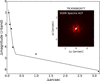 |
Fig. 2 5σ sensitivity limits and inset speckle auto-correlation function for the SOAR observation of TOI-4515 taken in the visible I-band. No nearby sources were detected within 3″ of the target star. |
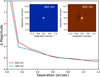 |
Fig. 3 Reconstructed NESSI speckle images and 5σ contrast limits from simultaneous diffraction-limited exposure sequences using the 562 nm filter on the blue camera and the 832 nm filter on the red camera. No nearby sources are detected. |
Stellar properties of TOI-4515.
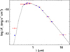 |
Fig. 4 Spectral energy distribution of TOI-4515. Red bars represent the observed photometric measurements, and the horizontal bars represent the effective width of the passband. Blue symbols are the model fluxes from the best-fit NextGen atmosphere model (black). |
3.2 Spectral energy distribution
As an independent determination of the basic stellar parameters, we performed an analysis of the broadband spectral energy distribution (SED) of the star together with the Gaia DR3 parallax (with no systematic offset applied; see, e.g., Stassun & Torres 2021) in order to determine an empirical measurement of the stellar luminosity and radius, following the procedures described in Stassun & Torres (2016); Stassun et al. (2017, 2018). We obtained the gri magnitudes from APASS, the JHKS magnitudes from 2MASS, the W1–W3 magnitudes from WISE, the GBPGRP magnitudes from Gaia, and the near-ultraviolet (NUV) magnitude from GALEX. Together, the available photometry spans the full stellar SED over the wavelength range 0.2–22 µm (see Fig. 4).
We performed a fit using NextGen stellar atmosphere models, with the free parameters being the Teff and the extinction AV, which we limited to the maximum line-of-sight value from the Galactic dust maps of Schlegel et al. (1998). We also adopted the metallicity determined from the spectroscopic analysis above. The resulting fit (Fig. 4) has a reduced χ2 of 0.9, excluding the GALEX NUV flux, which indicates a moderate level of activity (Findeisen et al. 2011), with AV = 0.03 ± 0.03 and Teff = 5335 ± 75 K. Integrating the (unreddened) model SED gives the bolo-metric flux at Earth, Fbol = 4.760 ± 0.055 × 10⁻¹⁰ erg s−1 cm−2. Taking the Fbol together with the Gaia parallax directly gives the bolometric luminosity, Lbol = 0.5573 ± 0.0068 L⊙, which with the Teff gives the stellar radius, R⋆ = 0.875 ± 0.025 R⊙. In addition, as a consistency check, we can estimate the stellar mass from the R⋆ together with the spectroscopically determined log 𝑔, giving M⋆ = 1.04 ± 0.10 M⊙.
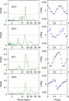 |
Fig. 5 Periodograms of the SuperWASP data for TOI-4515 in selected years (left) along with folds of the data on the 15.6 days rotational period (right). The horizontal line in the periodograms is the estimated 1% likelihood false-alarm level. |
3.3 Projected rotational velocity
From Teff, log 𝑔, ξ, and [Fe /H] fixed to the final values found in Sect. 3.1, we measured the stellar projected rotational velocity (υ sin i⋆) using the same MOOG code as above and applying the spectral synthesis of three regions around 5400, 6200, and 6700 Å. We adopted the same grid of model atmospheres as in Sect. 3.1 and, after fixing the macroturbulence velocity to the value of 2.5 km s^1 from the relationship by Brewer et al. (2016), we find a υ sin i⋆ of 3.4 + 0.5 km s−1. This value is compatible with the one calculated through Eq. (7) in Rainer et al. (2023), namely 3.6 + 0.5 km s−1.
3.4 Lithium abundance
We also derived the lithium abundance ALi from the measured lithium EW (<2.1 mÅ) and considering our stellar parameters previously derived together with the nonlocal thermodynamic equilibrium (NLTE) corrections by Lind et al. (2009). We could only obtain an upper limit of <0.5 dex on the lithium abundance. We obtain the same value also considering the synthesis analysis based on the MOOG code, after fixing the stellar parameters to those derived in Sects. 3.1 and 3.3. This upper limit supports an age of greater than that of the Hyades.
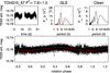 |
Fig. 6 Results of the periodogram analysis of the TESS photometry (Sector 57) of TOI-4515. Top-left panel: photometric time series. Red vertical lines indicate the epochs of primary and secondary minimum. Top-middle panel: GLS periodogram (solid black line) with the window function overplotted (dotted red line). Top-right panel: CLEAN periodogram. Bottom panel: TESS light curve phased with the primary periodogram periodicity, that is with the 7.6 days half stellar rotation period. |
3.5 Rotation period
We searched each year of the SuperWASP photometric data for a rotational modulation using methods outlined in Maxted et al. (2011). There is a persistent and highly significant periodicity with a period of 15.6 ± 0.3 days (see Fig. 5), where the error makes some allowance for phase shifts caused by changing star-spot patterns. The amplitude changes between years, varying between 5 mmag and l6 mmag.
We analyzed the photometric data time series from the four TESS Sectors separately and in a single combined series using the generalized Lomb-Scargle (GLS) and CLEAN periodograms, following the procedure described in Messina et al. (2022).
A highly significant periodicity is found at P = 7.64 ± 0.03 days in the combined series and similar periodicities, within the uncertainties, are detected in each single sector: P = 7.9 ± 1.2 days in Sector 17, P = 7.4 ± 0.5 days in the consecutive Sectors 45 and 46, P = 7.6 ± 1.0 days in Sector 57. As an example, a summary of the results from the periodogram analysis for Sector 57 are reported in Fig. 6. This periodicity is most likely linked to the rotation period of the star. As this periodicity is about half the rotation period derived from SuperWASP data (P = 15.6 days), we considered the possibility that the true period is twice the observed one. This circumstance may occur when dominant star spots of similar size occur on the stellar surface at longitude separated by about 180 deg, leading to similar features in the light curve on two occasions during one rotation period (double-dip variables). One example is represented by TOI-1807 (Nardiello et al. 2022; for a comprehensive discussion on period-doubling effects, see e.g., Collier Cameron et al. 2009). Whereas in the Sectors 17, 45, and 46, a gap in the data series prevented detection of the double dip, in the last Sector 57 it is quite clearly visible. More specifically, we see two consecutive minima of different depths separated by 7.6 days (marked by red ticks in Fig. 6), which supports our hypothesis of a true rotation period double as inferred from the periodogram analysis, that is P = 15.26 ± 0.06 days. This independent estimate from TESS data is in fair agreement with that from SuperWASP and with the rotation period expected on the basis of the rotation– chromospheric activity relation by Mamajek & Hillenbrand (2008; see Sect. 3.6). This rotation period also implies an age in agreement with the other age indicators analyzed in the present investigation, such as lithium (Sect. 3.4), chromospheric activity (Sect. 3.6), and kinematics (Sect. 3.7).
We also investigated the periodogram of the HARPS-N RV time-series, as well as several activity indicators ( , S-index, Bisector, CCF Contrast, CCF FWHM, chromospheric index CRX, differential line width dLw, H-alpha, and the sodium lines Na1 and Na2). Only the RV time series presents a peak at P ~ 7.5 days, albeit not significant, because the RV periodogram is dominated by the planetary signal.
3.6 Chromospheric activity
Ca II H&K emission was measured on HARPS-N spectra by exploiting the YABI tool, which is based on prescriptions by Lovis et al. (2011). The median value of the S index, calibrated into the Mount Wilson scale, is 0.357 ± 0.011. The corresponding log  is −4.67 ± 0.02. This value is at the lower edge of Hyades members of similar color. The expected rotation period using the Mamajek & Hillenbrand (2008) calibration is 13.4 days, which is very close to the rotation period measured in Sect. 3.5 and corresponds to an age of 1.0 Gyr. No X-ray observations are available for the target.
3.7 Kinematics
The space velocities U, V, and W, derived following the prescriptions by Johnson & Soderblom (1987), are listed in Table 1. These put the star slightly outside the kinematic locus of young stars defined by Eggen (1984), indicating an age of more than about 500 Myr and likely younger than the Sun.
3.8 Age
The stellar rotation period P = 15.5 ± 0.3 days obtained by combining the TESS and SuperWASP results allows a gyro-chronological age estimation of about 1.2 ± 0.2 Gyr according to Eqs. (12)–(14) in Mamajek & Hillenbrand (2008), with the uncertainty derived from the coefficient error propagation. This estimate is in good agreement with those from the independent methods applied by us; that is ≳0.6 Gyr from lithium, 1 Gyr from chromospheric activity, and ≳0.5 Gyr from kinematics. We therefore adopt a stellar age of 1.2 ± 0.2 Gyr.
3.9 Mass, radius, and system orientation
Isochrone fitting is inconclusive for age determination, as expected for an unevolved late G dwarf. The PARAM Bayesian Interface of PARSEC models4 (da Silva et al. 2006) yields 3.3 ± 3.2 Gyr. We used the same code to derive the stellar mass, allowing only the age range derived from indirect methods as in Desidera et al. (2015) and adopting the average between photometric and spectroscopic Teff. The resulting stellar mass is 0.949 ± 0.020 M⊙ (with the error being that provided by PARAM, systematic uncertainties in stellar models not included). The stellar radius was derived using the Stefan-Boltzmann law, as in Carleo et al. (2021), adopting the bolometric corrections given in the Mamajek tables to infer the stellar luminosity. The resulting stellar radius is 0.860 ± 0.030 R⊙, formally slightly smaller than but in agreement to better than 1σ with that derived from SED fitting (Sect. 3.2) and those adopted in TIC, PIC, and Gaia.
We derived a constraint on the stellar inclination angle by combining the measurements of the stellar radius, projected rotation velocity, and rotation period. For this purpose, we adopted R⋆ = 0.86 ± 0.03 R⊙, υ sin i⋆ = 3.4 ± 0.5 km s−1, and Prot = 15.3 ± 1.5 days. Although the photometric periodicity was determined with higher precision (see Sect. 3.5), here we enlarged the uncertainty to 10% to account for systematic effects such as differential rotation. With these values, υ = 2πR/Prot = 2.8 ± 0.3 km s−1, which is compatible with the measurement of v sin i⋆. Therefore, the inclination is consistent with 90 deg. To determine the lower limit on the inclination, we used the MCMC method advocated by Masuda & Winn (2020), which gave 2σ limits of cos i⋆ < 0.59 and an inclination of >54 deg. Therefore, the maximum difference in inclination angles between the star and planetary orbit is approximately 36 deg.
4 Planet validation
An alert regarding a planet candidate around TOI-4515 was released by the TESS Mission on 2021 October 21: indeed, the SPOC pipeline (Jenkins et al. 2016) at NASA Ames Research Center identified a candidate exoplanet with a period of 15.27 days. We used our independent data reduction of the FFIs to confirm the transits in the light curves and their planetary nature, following the approach described in Nardiello et al. (2020). First, we modeled and removed the stellar variability by interpolating to each light curve a fifth-order spline defined over a grid of knots at intervals of 13 h. We extracted the transit least squares (TLS) periodogram (Hippke & Heller 2019) of the light curve obtained by combining all the light curves after the suppression of the stellar activity. We found a peak in the TLS periodogram at P ~ 15.27 days with a strong signal detection efficiency (SDE ~24), confirming the presence of transit signals in the light curve.
Figure 7 illustrates the vetting tests we performed to validate the planetary nature of the candidate: from the folded the odd and even transits we demonstrate that, within the errors, the transit depths are in agreement, thus we can rule out the possibility that the object is an eclipsing binary with unequal components (panel b). We note a bump in the odd transits, but investigating this feature, we see that this bump is only clearly visible in one of the odd transits (the last one in time, and the most densely sampled), implying the possibility of the presence of a stellar spot during the observations. We also exclude any correlation between the X-and Y-positions of the star in the images and the transit signals, as demonstrated in panel c, and prove that there is no dependence between the transit depth and the photometric apertures available in our data reduction (panel d), minimizing the probability that the transit is due to a contaminating neighbor. The results of our data-validation tests are in agreement with those conducted by the SPOC.
We performed the analysis of the in- and out-of-transit cen-troid following the procedure described by Nardiello et al. (2020) as a final check to verify that the transit is on TOI-4515 and is not associated with a neighboring source. The results are reported in Fig. 8: each mean centroid, calculated for each sector, is in agreement within the errors with the position of TOI-4515. To ensure that our candidate is not a false positive (FP), we used the VESPA software (Morton 2012, 2015) as a conclusive verification step. We followed the procedure outlined in Mantovan et al. (2022), which takes into account the major concerns highlighted in Morton et al. (2023) and allows us to get reliable outcomes while using VESPA. We used our detrended long-cadence light curve (see Sect. 2.1.1), which we flattened using wotan and then phase folded. We find a 100% probability of having a Keplerian transiting companion orbiting TOI-4515, while the probability of an FP is very low, that is, approximately on the order of 1 × 10⁻⁹.
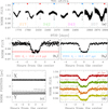 |
Fig. 7 Overview of the vetting of TOI-4515 b. Panel a shows the normalized light curve obtained from the long-cadence FFIs: red and blue triangles indicate the position of odd and even transits, respectively. BTJD is the Barycentric TESS Julian date, the time stamp measured in BJD, but offset by 2457000.0, i.e., BTJD = BJD – 2457000.0. Panels b are the odd and even transits folded by using the period of 15.27 days: the transit depths are in agreement between the odd and even transits, excluding the eclipsing binary nature of the target. Panel c shows the X- and Y-normalized positions of the stars (stellar positions subtracted by the mean stellar position) on the image phase-folded with the period of the candidate exoplanet. Squares represent X and triangles Y. No correlation with the transits is observed. Panel d illustrates the phased long-cadence light curves obtained with different photometric apertures: the mean transit depth is the same within the errors, confirming that the transit signals are not due to contaminants. |
5 Planetary system analysis
In order to retrieve the planetary system parameters, we performed a joint fit with RV and transit data using the package PyORBIT5 (Malavolta et al. 2016, 2018). We took into account the effects of stellar activity and astrophysical contaminants. The transit modeling relies on the package batman (Kreidberg 2015) with the addition of a local polynomial trend for each transit. We also added a Gaussian process (GP) in the RV fit using the package george (Ambikasaran et al. 2015) in order to fit the stellar activity with a quasi-periodic kernel as defined by Grunblatt et al. (2015), with h representing the amplitude of the correlations, θ the rotation period of the star, ω the length scale of the periodic component (related to the size evolution of the active regions), and λ the correlation decay timescale.
We modeled the TESS, KeplerCam, and LCO CTIO light curves including the following parameters: the time of first inferior conjunction Tc, the orbital period P, the eccentricity e, and argument of periastron ω with the parametrization from Eastman et al. (2013;  ), the quadratic limb darkening (LD) coefficients with Kipping (2013) parametrization, the impact parameter b, and the scaled planetary radius RP/R⋆. During the short duration of a transit, stellar activity due to stellar rotation can be approximated with a quadratic trend without consequences on the derived stellar parameters (Benatti et al. 2019; Carleo et al. 2021). This is computationally more efficient than modeling the full light curve with a Gaussian process when only a few transits are observed, as in the case of TOI-4515b. We therefore included a polynomial trend in the modelling of each of the observed transits. Moreover, we imposed a Gaussian prior on the stellar density using the stellar mass and radius provided in Sect. 3.9, and Gaussian priors for the limb darkening coefficients obtained with the code PyLDTk6 (Parviainen & Aigrain 2015; Husser et al. 2013). We increased the limb darkening errors in order to avoid significant deviations between measured and predicted limb darkening coefficients, especially in TESS light curves, as explained in Patel & Espinoza (2022). We considered the impact parameter b as a free parameter (e.g., Frustagli et al. 2020). As the possible contaminating sources are negligible (Fig. 1), the dilution factor is not included in the fit.
Regarding the RV data, we added offset and jitter terms in order to take into account the offsets among the three different instruments and possible systematic errors and short-term stellar activity noise. When including a Gaussian process to model the activity, we also imposed a Gaussian prior on the rotational period with the value obtained from the photometric analysis (see Table 1). To explore the parameter space we used the dynamic nested sampler dynesty7 (Speagle 2020; Koposov et al. 2022) to sample the parameter space, with 1000 live points. We tested 12 models, resulting from the combination of: (i) one or two planets; (ii) with and without GP; and (iii) no trend, a linear trend, or a quadratic trend. We investigated the trend in order to rule out possible long-period additional companions, even though the RV data do not show any evident trend. We also computed the Bayesian evidence log 𝒵 from the nested sampling in order to evaluate the quality of our fits (see Bayesian values in Table 2). The difference in log 𝒵 between the models with no trend is not significant; a small increase in the Bayesian evidence with an increase in the complexity of the model is expected even for nonfavored models (e.g., Faria et al. 2016).
The planetary system parameters obtained with the two 1p and 1p+GP models with no trend are listed in Table 3, while the RV and transit fits with the overplotted models obtained from the model with GP are represented in Fig. 9. We find TOI-4515 b to have a mass of 2.03 ± 0.05 MJ and a radius of 1.09 ± 0.04 RJ, with an orbital period of 15.27 d and an eccentricity of 0.46 ± 0.01. The rotational period found by the model with the GP is 15.84 days. Although this value is close to the orbital period, it is not consistent with it within 1σ (further discussion about the similar periods is given in Sect. 7.2). However, the model without the modeling of the activity through the GP gives very similar results, meaning that the activity is not relevant in the determination of the system parameters, such as planetary mass. The median value of the posterior of the rotational period of the star is 15.84 days, which is apparently higher than the imposed prior, albeit well consistent within one sigma. The origin of this discrepancy may actually reside in the relatively small amplitude of stellar activity (around 10–20 ms−1) compared to the planetary signal (190 m s−1) combined with the reduced number of data collected, which causes some difficulties in modeling the activity signal in the data. In principle, the similarity between the orbital period of the planet and the stellar rotation period of the star may affect some parameter estimations, especially eccentricity and RV semi-amplitude; for example, the RV curve may be distorted by the distribution of active regions on the surface of the star, which appears in phase with the orbit. For this specific system, all of our tests confirmed that the derived planetary parameters are insensitive to the specific activity modeling. To highlight this fact, we reported in Table 2 the less-constrained activity model among the many tested (e.g., no training on other datasets or use of multidimensional GPs; see Nardiello et al. 2022).
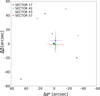 |
Fig. 8 Analysis of the in- and out-of-transit centroid of TOI-4515 b. Within the errors, the centroid coordinates coincide with the target position (located in (0,0)). |
6 Constraints on additional companions, both nearby and distant
A significant fraction of WJ systems have been found to host additional nearby or distant planetary companions (Huang et al. 2016; Bryan et al. 2016; Wu et al. 2023). In order to constrain the presence of additional companions, we considered the various data collected for the object (photometry, RV, and imaging, Sect. 2) as well as archival astrometric data.
To determine the precise mid-transit times and search for transit timing variations (TTVs), we conducted a global fit on the RV and transit data using allesfitter (Günther & Daylan 2021). In the fitting process, we employed Gaussian priors on T0,  , a/R⋆ and transformed LD coefficients (q1 and q2)8. These parameters were sourced from Table 3. For each transit, we applied an additional second-order polynomial function to account for potential trends. We employed the same method and setup as in Sect. 5 to sample the parameter space, resulting in at least 400 independent samples. Subsequently, we fit a linear ephemeris to the transit mid-times using the Markov chain Monte Carlo (MCMC) method. We optimized the reference epoch to minimize the covariance between T0 and Porb. The resulting transit mid-times and their deviations from the linear ephemeris are listed in Table 4. The residuals between the observed and predicted transit mid-times, as determined by the linear ephemeris, are shown in Fig. 10. There is no significant TTV signal, as all residuals with errors are consistent with zero deviation from the linear ephemeris within a 2σ confidence level.
We also tested the presence of additional nontransiting companions, deriving the detection limits from the HARPS-N RV time series. To compute the detection limits, we adopted the Bayesian technique described in Pinamonti et al. (2022), taking into account the results of the RV and photometric data joint modeling as priors for the orbital period, Porb, and transit epoch, T0, as these would be difficult to precisely constrain without the transit analysis. The resulting detection map is shown in Fig. 11. The detection map shows how it is currently impossible to constrain the presence of additional sub-Neptune companions (Mp sin / < 20 M⊕), even at very short periods. We instead can exclude the presence of Saturn-mass planets at periods shorter than 40 ± 5 d.
Moving to slightly larger separations, we simulated the presence of companions able to reproduce the observed renormalized unit weight error (RUWE) from Gaia DR3 (1.09), following the procedure described in Blanco-Pozo et al. (2023). Brown dwarf companions of various masses are ruled out in the range 1–4 au, as shown in Fig. 12.
We also considered the imaging datasets described in Sect. 2 and Gaia DR3. No stellar companions (comoving objects) were found in Gaia DR3 within 120 arcsec (more than 20 000 au at the distance of the star). The typical detection limits of close companions from Gaia are taken from Brandeker & Cataldi (2019). The detection limits from Sect. 2.3 and Gaia were transformed into mass limits using the Baraffe et al. (2015) models. The combined detection limits are shown in Fig. 13. The allowed space for undetected companions is rather large, even in the stellar regime.
Finally, we checked for indications of the presence of companions from the presence of differences in the proper motion at various epochs. As our target is not included in the HIP-PARCOS catalog, we considered long-baseline catalogs such as Tycho2 (Høg et al. 2000), PPMXL (Roeser et al. 2010), and UCAC5 (Zacharias et al. 2017), and compared the long-term proper motions from these catalogues with the short-term proper motions from Gaia DR3. Marginally significant differences are found for Tycho2 and PPMXL catalogs. We estimated the mass and projected separation for companions that could be responsible of the Gaia-Tycho2 proper motion difference using the COPAINS code (Fontanive et al. 2019). Figure 13 shows the results considering appropriate distributions of the orbital parameters. However, we caution that, while formally significant at 2–3 σ, the observed difference may also be due to systematic uncertainties in the proper motions in pre-Gaia catalogs, as described, for example, by Lindegren et al. (2016) and Shi et al. (2019). Therefore, we do not consider this as conclusive evidence of the presence of a companion with the characteristics shown in Fig. 13. We also note that, at a separation of larger than about 30 au, the presence of a companion with the characteristics expected for the nominal Gaia-Tycho2 proper motion difference is ruled out by the imaging data.
We conclude that available data do not support the presence of additional companions, although the current detection limits allow for low-mass companions even in the stellar regime at separations of greater than about 10 au.
Comparison between the joint models.
TOI-4515 parameters from the transit and RV joint fit, obtained with models 1p and 1p+GP with no trend.
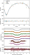 |
Fig. 9 Upper panel: HARPS-N (blue points), TRES (orange), and FEROS (green) RV data with the overplotted fit from the 1p model. Lower panel: from top to bottom, TESS transits from Sectors 17 (long cadence), 42 (2 transits), 43, and 57, and LCO and KeplerCam light curves. The black line is the inferred 1p model. |
Optimized epochs, transit mid-times, their uncertainties, and deviations from the linear ephemeris for each transit.
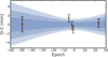 |
Fig. 10 Observed minus calculated transit mid-times by linear ephemeris. The blue regions, from inner to outer, represent the propagation of ±1σ, ±2σ, and ±3σ errors associated with the calculated orbital period. No statistically significant TTVs are detected at levels of ±2σ. |
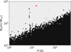 |
Fig. 11 Detection function map of the RV time series of TOI-4515. The gray part corresponds to the area in the period–minimum mass space, where additional signals could be detected if present in the data, while the black region corresponds to the area where the detection probability is negligible. The red dot represents TOI-4515 b, for reference. At around P = 7.5 d, there are some low-sensitivity spots even at large masses, which are caused by the 1/2 aliases of Prot and Porb. |
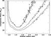 |
Fig. 12 Limits on the presence of companions around TOI-4515 from the Gaia RUWE. The short-dashed, dashed-dotted, and long-dashed correspond to probabilities of 90%, 95%, and 99%, respectively, of getting a RUWE larger than the observed value. |
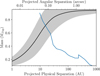 |
Fig. 13 Constraints on the presence of companions from direct imaging and Gaia-Tycho2 proper motion differences. The detection limits from direct imaging, combining various datasets at different projected separations, are shown as a blue continuous line (the <200 AU region of the blue line comes from the speckle interferometry). The continuous black line shows the expected mass and projected separation of companions compatible with the nominal Gaia-Tycho2 proper motion difference, while the shaded gray area shows the lσ limits considering realistic distributions of orbital parameters. |
7 Discussion
The discovery of TOI-4515 b, a WJ with an orbital period of ~15 days, a mass of two Jupiter masses, and an eccentricity of 0.46, orbiting a solar mass star with a metallicity of 0.05, offers insights into the diverse formation and dynamical histories of WJs, and sheds light on the mechanisms responsible for the excitement of their eccentricities. Considering the slightly metal-rich nature of its host star (~10% above solar metallicity), it is a possibility that multiple gas giants formed within the system (Fischer & Valenti 2005; Wu et al. 2023). After the gaseous disk dissipated, these gas giants may have experienced interactions, such as planet-planet scattering (Anderson et al. 2020) or secular interactions (Dawson & Chiang 2014; Petrovich & Tremaine 2016; Dong et al. 2014; Naoz 2016), that led to the excitation of TOI-4515 b’s eccentric orbit. Such dynamical scenarios are supported by the analysis of the normalized angular momentum deficit (NAMD) of TOI-4515 b (Turrini et al. 2020, 2022; Carleo et al. 2021). In the case of single-planet systems, the NAMD can be expressed solely as a function of the orbital eccentricity and the spin-orbit misalignment, where neglecting the unknown contribution of the latter provides a lower bound to the dynamical excitation of the system. This lower bound to the TOI-4515 b NAMD is 0.11, which is about two orders of magnitude higher than the NAMD of the Solar System (1.3 × 10⁻³; Turrini et al. 2020). This high value is clearly in the regime of intense chaotic evolution (Turrini et al. 2022) and is suggestive of catastrophic collisional events (Rickman et al. 2023).
Further clues as to the dynamical past of TOI-45l5b are supplied by its orbital and physical characteristics. First, the periastron of the system is too large to initiate tidal migration, suggesting that TOI-4515 b did not undergo eccentric migration unless it is still dynamically coupled with companions that possess enough mass and that are sufficiently nearby to suppress the effects of general relativity, thereby sustaining the eccentricity oscillation of the WJ (Wu & Murray 2003). Second, as no additional companion has been detected (as described in the following section), the eccentricity of TOI-4515 b might be a relic of violent scattering events occurring in the distant past (Anderson et al. 2020) that caused the dynamical or colli-sional removal of the original companion(s). Such a scenario is supported by the high density of the giant planet.
The density of TOI-4515 b is about 1.5 times that of Jupiter, which in turn is three times more metallic than its host star (Atreya et al. 2018) because of the accretion of planetary material together with gas during its formation (e.g., Alibert et al. 2018; Öberg & Wordsworth 2019). This comparison suggests that the high density of TOI-4515 b could arise from the inges-tion of one or more of its original planetary companions during the dynamical instability that generated its eccentricity. If this is the case, the system may still be spin–orbit aligned (Wang et al. 2021; Rice et al. 2022), because scattering is less effective in exciting mutual inclination compared to the secular process, while collisions have damping effects on the dynamical excitation of planets (Chambers 2001). In this sense, measuring the Rossiter-McLaughlin effect for TOI-4515 b (estimated to be ~26 m s−1 from eq. 40 in Winn 2010) would offer further insights into the dynamic history and formation processes of WJs like TOI-4515b.
7.1 Photoevaporation modeling
In order to investigate the hydrodynamic stability of TOI-4515 b, we employed our model presented in Locci et al. (2019) and updated for studying the evolution of planets spanning from Jovian-sized to sub-Neptunian-sized bodies (Benatti et al. 2021; Maggio et al. 2022; Damasso et al. 2023; Naponiello et al. 2023). In this work, we investigated the photo-evaporation of the planetary atmosphere using the energy-limited approximation (Erkaev et al. 2007), and taking into account the evolution of the X-ray and EUV luminosity (Penz et al. 2008; Sanz-Forcada et al. 2011). The time variation of the planetary radius, which evolves in response to both gravitational contraction and mass loss, is described using the theoretical model proposed by Fortney et al. (2007). By evaluating the Jeans escape parameter A = GmHMP/kBTeqRP (e.g., Fossati et al. 2017), we verified that the planet is stable against hydrodynamic evaporation at the present age, mostly because of its high mass. More specifically, we obtained Λ ~ 575, which is much larger than the critical value of Λc = 80 for a significant atmospheric escape, and therefore the hydrodynamic mass loss rate should be negligible. We also investigated the history of the planet in order to determine whether or not the mass and radius measured today could be the result of photo-evaporation at early ages (back in time to 10 Myr). We were not able to find any plausible planet configuration with Λ < Λc. This condition could be reached only assuming that the planet had a radius of more than a factor 7 larger than the present value - keeping its mass fixed –, but a young evaporating planet should also be more massive and with a lower equilibrium temperature. We conclude that TOI-4515 b was also stable against photoevaporation in the past, in spite of the greater high-energy irradiation.
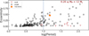 |
Fig. 14 Distribution of eccentricities as a function of the orbital period for Jupiter-sized planets. The dashed blue line represents the ten-day boundary between HJs and WJs. The orange point represents TOI-4515 b. The red triangles represent the planets in multi-planetary systems. Data taken as of UT 2023 September 24. |
7.2 Eccentricity and companionship
To frame the orbital characteristics of TOI-4515 in the context of the population of close-in giant planets, we made use of the TEPCat catalog (Southworth 2011)9 to selected planets with orbital periods within 0 < Porb < 200 days, eccentricities with uncertainties smaller than 0.1, and planetary mass precision of better than 50%, and mass falling in the range between 0.20 and 12 MJ (Jupiter-sized planets). The resulting planets encompass both the HJ and WJ populations and are represented in Fig. 14, where we see that HJs with orbital periods of below 3 days are all characterized by circular orbits, which is likely due to the effective tidal dissipation that they experience throughout their lives. For increasing orbital periods, we see the appearance of giant planets on eccentric orbits alongside those on circular orbits and we see that their maximum eccentricity increases with orbital period. This trend can be intuitively explained by the rapid decrease in tidal circularization rate with increasing orbital distance (see Jackson et al. 2008, Eq. (1)), which suggests that the farther out the planet from its host star, the more likely it is that its primordial eccentricity will be preserved, at least partially. TOI-4515 b, with its orbital period of 15 days, radius of ~1.1 RJ, mass of ~2 MJ, and eccentricity of 0.46, lies in the region of high-eccentricity WJs and its orbital eccentricity is close to the high-end tail of giant planets at similar orbital distances. The eccentricity is probably the remnant of an episode of planet-planet scattering that excited the eccentricity and also brought the planet close to the star. The tidal interaction with the star is acting to damp the primordial higher eccentricity and its circularization timescale.
In order to better understand the origin of the eccentricity of TOI-4515 b, we calculated the circularization timescale. An estimate of the tidal circularization timescale τe (e-folding time for the decay of the eccentricity) can be made with the tidal model of Leconte et al. (2010), where the modified tidal quality factors of the star  and of the planet
  are used instead of the time lag. The approximate relationship
  has been adopted, where k2 s,p is the Love number of degree 2, ∆ts,p is the time lag, n = 2π/Porb the orbital mean motion, and the subscript s or p refers to the star or the planet, respectively. The circularization timescale depends mostly on the dissipation of the tides inside the planet with a secondary contribution from the dissipation inside the star. Adopting
  , which is similar to the value found in the case of Jupiter by modelling the orbital evolution of the Galilean moons (Ogilvie 2014), we find τe ~ 7 Gyr, which suggests that the eccentricity of TOI-45l5b could be primordial. However, a smaller value of
  cannot be excluded given our ignorance of the internal structure of TOI-4515b and our limited understanding of tidal dissipation in giant planets. For example, with
  , which was suggested in the case of Saturn by Sinclair (1983), we find τe ~ 0.9 Gyr, implying that the present eccentricity could require some form of excitation along the lifetime of the system. A value of
  as small as 104 could be observationally tested by future measurements of the night-side temperature of the planet. Specifically, as a consequence of the rather high eccentricity and low
  , the power dissipated inside the planet by the tides is predicted to be of ~2.6 × 10²⁰ W, which would imply an effective temperature of ~500 K assuming a uniform black-body irradiation from the whole surface of the body. On the other hand, the equilibrium temperature of the planet, assuming zero albedo, is ~730 K, implying that the tidal power is ~24% of that received by the planet from its host star. Another consequence of the eccentric orbit is the pseudosyn-chronization of the planet, which is expected to rotate with a period of 6.2 days because of the stronger tidal interaction at periastron. It is interesting to note that the stellar rotation period is close to the orbital period of TOI-4515 b. This could simply be a coincidence, but it could also point to some kind of star– planet interaction as suggested by for example Lanza (2O22a,b). The stellar synchronization timescale is longer than the age of the Universe, even assuming
  , which would imply an extremely strong tidal dissipation inside the star, which is not predicted by current tidal models (Ogilvie 2014; Barker 2020). Therefore, tides are not expected to significantly affect the stellar rotational evolution in this system. This also applies to the obliquity of the system, which is not expected to vary over its lifetime, even assuming
  . Therefore, a measurement of the Rossiter-McLaughlin effect can provide useful information on the formation of this system (cf. Sect. 7).
8 Conclusions
In this paper, we present the discovery and mass determination of an eccentric WJ transiting TOI-4515 ( TYC 1203-01161-1, TIC 456862677) and observed by TESS in Sectors 17, 42, 43, and 57. We collected photometric (TESS, WASP, KeplerCam, CALOU, LCOGT), spectroscopic (HARPS-N, TRES, FEROS), and high-contrast imaging (SOAR, NESSI) data and constrained most of the stellar and planetary parameters. TOI-4515 is a relatively young star with an age of 1.2 ± 0.2 Gyr and an effective temperature of about 5400 K, falling in the G-type category. We obtained a stellar rotational period of 15.5 ± 0.3 days from a combined TESS and WASP analysis. The giant planet has a mass of 2.005 ± 0.052MJ, a radius of 1.086 ± 0.039 MJ, and an orbital period of 15.266446 ± 0.000013 days. Its eccentricity of 0.461 ± 0.007 places it among the sample of WJs with eccentric orbits. The combination of the eccentric orbit and a large periastron suggests planet-planet interactions, but from the available data, the presence of additional companions is not supported. However, the loss of primordial planetary companions is consistent with the high NAMD and high density of TOI-4515 b, which jointly suggest a violent dynamical past characterized by planetary collisions. Additional data, such as imaging with the extreme-AO instruments and/or measurement of the Rossiter-McLaughlin effect, are needed in order to make major improvements and further inferences as to the architecture of the system.
Acknowledgements
This work has been supported by the PRIN-INAF 2019 “Planetary systems at young ages (PLATEA)” and ASI-INAF agreements no. 2018-16-HH.0 and 2021-5-HH.0. This work made use of tpfplotter by J. Lillo-Box (publicly available in www.github.com/jlillo/tpfplotter), which also made use of the python packages astropy, lightkurve, matplotlib and numpy. Some of the observations in this paper made use of the NN-EXPLORE Exoplanet and Stellar Speckle Imager (NESSI). NESSI was funded by the NASA Exoplanet Exploration Program and the NASA Ames Research Center. NESSI was built at the Ames Research Center by Steve B. Howell, Nic Scott, Elliott P. Horch, and Emmett Quigley. This work makes use of observations from the LCOGT network. This research has made use of the Exoplanet Follow-up Observation Program (ExoFOP; DOI: 10.26134/ExoFOP5) website, which is operated by the California Institute of Technology, under contract with the National Aeronautics and Space Administration under the Exoplanet Exploration Program. We acknowledge the use of public TESS data from pipelines at the TESS Science Office and at the TESS Science Processing Operations Center. Resources supporting this work were provided by the NASA High-End Computing (HEC) Program through the NASA Advanced Supercomputing (NAS) Division at Ames Research Center for the production of the SPOC data products. Funding for the TESS mission is provided by NASA’s Science Mission Directorate. K.A.C. acknowledges support from the TESS mission via subaward s3449 from MIT. D.D. acknowledges support from the NASA Exoplanet Research Program grant 18-2XRP18_2-0136. Based in part on observations obtained at the Southern Astrophysical Research (SOAR) telescope, which is a joint project of the Ministério da Ciência, Tecnologia e Inovações (MCTI/LNA) do Brasil, the US National Science Foundation’s NOIRLab, the University of North Carolina at Chapel Hill (UNC), and Michigan State University (MSU). A.J. acknowledges support from ANID – Millennium Science Initiative – ICN12_009 and from FONDECYT project 1210718. R.B. acknowledges support ANID – Millennium Science Initiative – ICN12_009 and from FONDECYT project 11200751. S.Q. acknowledges support from the TESS GI Program under award 80NSSC21K1056 and from the TESS mission via subaward s3449 from MIT. D.D. acknowledges support from the NASA Exoplanet Research Program grant 18-2XRP18_2-0136, and from the TESS Guest Investigator Program grants 80NSSC22K1353 and 80NSSC22K0185. S.W. gratefully acknowledges the generous support from the Heising-Simons Foundation, including support from Grant 2023-4050.
Appendix A RVs
Time series of TOI-4515 from HARPS-N, TRES, and FEROS data: Julian dates, RVs, and their related uncertainties. For HARPS-N data the  values are listed as well.
Appendix B Corner plot
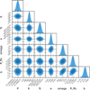 |
Fig. B.1 Corner plot of the posterior distributions for the planetary parameters obtained with the 1p+GP model. |
References
- Albrecht, S. H., Dawson, R. I., & Winn, J. N. 2022, PASP, 134, 082001 [NASA ADS] [CrossRef] [Google Scholar]
- Alibert, Y., Venturini, J., Helled, R., et al. 2018, Nat. Astron., 2, 873 [NASA ADS] [CrossRef] [Google Scholar]
- Aller, A., Lillo-Box, J., Jones, D., Miranda, L. F., & Barceló Forteza, S. 2020, A&A, 635, A128 [NASA ADS] [CrossRef] [EDP Sciences] [Google Scholar]
- Ambikasaran, S., Foreman-Mackey, D., Greengard, L., Hogg, D. W., & O’Neil, M. 2015, IEEE Trans. Pattern Anal. Mach. Intell., 38, 252 [Google Scholar]
- Anderson, K. R., Lai, D., & Pu, B. 2020, MNRAS, 491, 1369 [NASA ADS] [CrossRef] [Google Scholar]
- Atreya, S. K., Crida, A., Guillot, T., et al. 2018, in Saturn in the 21st Century, eds. K. H. Baines, F. M. Flasar, N. Krupp, & T. Stallard, 5 [CrossRef] [Google Scholar]
- Baraffe, I., Homeier, D., Allard, F., & Chabrier, G. 2015, A&A, 577, A42 [NASA ADS] [CrossRef] [EDP Sciences] [Google Scholar]
- Baratella, M., D’Orazi, V., Biazzo, K., et al. 2020, A&A, 640, A123 [NASA ADS] [CrossRef] [EDP Sciences] [Google Scholar]
- Barker, A. J. 2020, MNRAS, 498, 2270 [Google Scholar]
- Benatti, S., Nardiello, D., Malavolta, L., et al. 2019, A&A, 630, A81 [NASA ADS] [CrossRef] [EDP Sciences] [Google Scholar]
- Benatti, S., Damasso, M., Borsa, F., et al. 2021, A&A, 650, A66 [NASA ADS] [CrossRef] [EDP Sciences] [Google Scholar]
- Blanco-Pozo, J., Perger, M., Damasso, M., et al. 2023, A&A, 671, A50 [NASA ADS] [CrossRef] [EDP Sciences] [Google Scholar]
- Brahm, R., Jordán, A., Bakos, G. Á., et al. 2016, AJ, 151, 89 [Google Scholar]
- Brahm, R., Jordán, A., & Espinoza, N. 2017, PASP, 129, 034002 [Google Scholar]
- Brandeker, A., & Cataldi, G. 2019, A&A, 621, A86 [NASA ADS] [CrossRef] [EDP Sciences] [Google Scholar]
- Brewer, J. M., Fischer, D. A., Valenti, J. A., & Piskunov, N. 2016, ApJS, 225, 32 [Google Scholar]
- Brown, T. M., Baliber, N., Bianco, F. B., et al. 2013, PASP, 125, 1031 [Google Scholar]
- Bryan, M. L., Knutson, H. A., Howard, A. W., et al. 2016, ApJ, 821, 89 [NASA ADS] [CrossRef] [Google Scholar]
- Buchhave, L. A., Bakos, G. Á., Hartman, J. D., et al. 2010, ApJ, 720, 1118 [NASA ADS] [CrossRef] [Google Scholar]
- Buchhave, L. A., Latham, D., Johansen, A., et al. 2012, Nature, 486, 375 [NASA ADS] [CrossRef] [Google Scholar]
- Buchhave, L. A., Bizzarro, M., Latham, D. W., et al. 2014, Nature, 509, 593 [Google Scholar]
- Carleo, I., Malavolta, L., Lanza, A. F., et al. 2020, A&A, 638, A5 [NASA ADS] [CrossRef] [EDP Sciences] [Google Scholar]
- Carleo, I., Desidera, S., Nardiello, D., et al. 2021, A&A, 645, A71 [EDP Sciences] [Google Scholar]
- Casagrande, L., Ramírez, I., Meléndez, J., Bessell, M., & Asplund, M. 2010, A&A, 512, A54 [NASA ADS] [CrossRef] [EDP Sciences] [Google Scholar]
- Castelli, F., & Kurucz, R. L. 2003, in Modelling of Stellar Atmospheres, 210, eds. N. Piskunov, W. W. Weiss, & D. F. Gray, A20 [NASA ADS] [Google Scholar]
- Chambers, J. E. 2001, Icarus, 152, 205 [Google Scholar]
- Collier Cameron, A., Davidson, V. A., Hebb, L., et al. 2009, MNRAS, 400, 451 [NASA ADS] [CrossRef] [Google Scholar]
- Collins, K. A., Kielkopf, J. F., Stassun, K. G., & Hessman, F. V. 2017, AJ, 153, 77 [Google Scholar]
- Cosentino, R., Lovis, C., Pepe, F., et al. 2014, SPIE Conf. Ser., 9147, 91478C [Google Scholar]
- Covino, E., Esposito, M., Barbieri, M., et al. 2013, A&A, 554, A28 [NASA ADS] [CrossRef] [EDP Sciences] [Google Scholar]
- Damasso, M., Locci, D., Benatti, S., et al. 2023, A&A, 672, A126 [NASA ADS] [CrossRef] [EDP Sciences] [Google Scholar]
- da Silva, L., Girardi, L., Pasquini, L., et al. 2006, A&A, 458, 609 [NASA ADS] [CrossRef] [EDP Sciences] [Google Scholar]
- Dawson, R. I., & Chiang, E. 2014, Science, 346, 212 [Google Scholar]
- Dawson, R. I., & Johnson, J. A. 2018, ARA&A, 56, 175 [Google Scholar]
- Dawson, R. I., Johnson, J. A., Morton, T. D., et al. 2012, ApJ, 761, 163 [NASA ADS] [CrossRef] [Google Scholar]
- Desidera, S., Covino, E., Messina, S., et al. 2015, A&A, 573, A126 [NASA ADS] [CrossRef] [EDP Sciences] [Google Scholar]
- Dong, S., Katz, B., & Socrates, A. 2014, ApJ, 781, L5 [Google Scholar]
- Dong, J., Huang, C. X., Dawson, R. I., et al. 2021a, ApJS, 255, 6 [NASA ADS] [CrossRef] [Google Scholar]
- Dong, J., Huang, C. X., Zhou, G., et al. 2021b, ApJ, 920, L16 [NASA ADS] [CrossRef] [Google Scholar]
- Dong, J., Wang, S., Rice, M., et al. 2023, ApJ, 951, L29 [NASA ADS] [CrossRef] [Google Scholar]
- Dutra-Ferreira, L., Pasquini, L., Smiljanic, R., Porto de Mello, G. F., & Steffen, M. 2016, A&A, 585, A75 [NASA ADS] [CrossRef] [EDP Sciences] [Google Scholar]
- Eastman, J., Gaudi, B. S., & Agol, E. 2013, PASP, 125, 83 [Google Scholar]
- Eggen, O. J. 1984, AJ, 89, 830 [NASA ADS] [CrossRef] [Google Scholar]
- Erkaev, N. V., Kulikov, Y. N., Lammer, H., et al. 2007, A&A, 472, 329 [NASA ADS] [CrossRef] [EDP Sciences] [Google Scholar]
- Faria, J. P., Haywood, R. D., Brewer, B. J., et al. 2016, A&A, 588, A31 [NASA ADS] [CrossRef] [EDP Sciences] [Google Scholar]
- Findeisen, K., Hillenbrand, L., & Soderblom, D. 2011, AJ, 142, 23 [Google Scholar]
- Fischer, D. A., & Valenti, J. 2005, ApJ, 622, 1102 [NASA ADS] [CrossRef] [Google Scholar]
- Fontanive, C., Mužic, K., Bonavita, M., & Biller, B. 2019, MNRAS, 490, 1120 [NASA ADS] [CrossRef] [Google Scholar]
- Fortney, J. J., Marley, M. S., & Barnes, J. W. 2007, ApJ, 659, 1661 [Google Scholar]
- Fossati, L., Erkaev, N. V., Lammer, H., et al. 2017, A&A, 598, A90 [NASA ADS] [CrossRef] [EDP Sciences] [Google Scholar]
- Frustagli, G., Poretti, E., Milbourne, T., et al. 2020, A&A, 633, A133 [NASA ADS] [CrossRef] [EDP Sciences] [Google Scholar]
- Fűrész, G. 2008, PhD thesis, University of Szeged, Hungary [Google Scholar]
- Fűrész, G., Szentgyorgyi, A. H., & Meibom, S. 2008, in Precision Spectroscopy in Astrophysics, eds. N. C. Santos, L. Pasquini, A. C. M. Correia, & M. Romaniello, 287 [Google Scholar]
- Grunblatt, S. K., Howard, A. W., & Haywood, R. D. 2015, ApJ, 808, 127 [NASA ADS] [CrossRef] [Google Scholar]
- Guerrero, N. M., Seager, S., Huang, C. X., et al. 2021, ApJS, 254, 39 [NASA ADS] [CrossRef] [Google Scholar]
- Günther, M. N., & Daylan, T. 2021, ApJS, 254, 13 [CrossRef] [Google Scholar]
- Gupta, A. F., Jackson, J. M., Hebrard, G., et al. 2023, AJ, 165, 234 [NASA ADS] [CrossRef] [Google Scholar]
- Hippke, M., & Heller, R. 2019, A&A, 623, A39 [NASA ADS] [CrossRef] [EDP Sciences] [Google Scholar]
- Høg, E., Fabricius, C., Makarov, V. V., et al. 2000, A&A, 355, L27 [Google Scholar]
- Howell, S. B., Everett, M. E., Sherry, W., Horch, E., & Ciardi, D. R. 2011, AJ, 142, 19 [Google Scholar]
- Huang, C., Wu, Y., & Triaud, A. H. M. J. 2016, ApJ, 825, 98 [NASA ADS] [CrossRef] [Google Scholar]
- Huang, C. X., Vanderburg, A., Pál, A., et al. 2020a, RNAAS, 4, 204 [Google Scholar]
- Huang, C. X., Vanderburg, A., Pál, A., et al. 2020b, RNAAS, 4, 206 [NASA ADS] [Google Scholar]
- Hunter, A. A., Macgregor, A. B., Szabo, T. O., Wellington, C. A., & Bellgard, M. I. 2012, Source Code Biol. Med., 7, 1 [Google Scholar]
- Husser, T.-O., Wende-von Berg, S., Dreizler, S., et al. 2013, A&A, 553, A6 [NASA ADS] [CrossRef] [EDP Sciences] [Google Scholar]
- Jackson, B., Greenberg, R., & Barnes, R. 2008, ApJ, 678, 1396 [Google Scholar]
- Jenkins, J. M. 2002, ApJ, 575, 493 [Google Scholar]
- Jenkins, J. M., Chandrasekaran, H., McCauliff, S. D., et al. 2010, SPIE Conf. Ser., 7740, 77400D [Google Scholar]
- Jenkins, J. M., Twicken, J. D., McCauliff, S., et al. 2016, SPIE Conf. Ser., 9913, 99133E [Google Scholar]
- Jenkins, J. M., Tenenbaum, P., Seader, S., et al. 2020, Kepler Data Processing Handbook: Transiting Planet Search, Kepler Science Document KSCI-19081-003 [Google Scholar]
- Johnson, D. R. H., & Soderblom, D. R. 1987, AJ, 93, 864 [Google Scholar]
- Kaufer, A., Stahl, O., Tubbesing, S., et al. 1999, The Messenger, 95, 8 [Google Scholar]
- Kipping, D. M. 2013, MNRAS, 435, 2152 [Google Scholar]
- Koposov, S., Speagle, J., Barbary, K., et al. 2022, https://zenodo.org/records/7388523 [Google Scholar]
- Kreidberg, L. 2015, PASP, 127, 1161 [Google Scholar]
- Lanza, A. F. 2022a, A&A, 658, A195 [NASA ADS] [CrossRef] [EDP Sciences] [Google Scholar]
- Lanza, A. F. 2022b, A&A, 665, A47 [NASA ADS] [CrossRef] [EDP Sciences] [Google Scholar]
- Leconte, J., Chabrier, G., Baraffe, I., & Levrard, B. 2010, A&A, 516, A64 [NASA ADS] [CrossRef] [EDP Sciences] [Google Scholar]
- Li, J., Tenenbaum, P., Twicken, J. D., et al. 2019, PASP, 131, 024506 [NASA ADS] [CrossRef] [Google Scholar]
- Lind, K., Asplund, M., & Barklem, P. S. 2009, A&A, 503, 541 [NASA ADS] [CrossRef] [EDP Sciences] [Google Scholar]
- Lindegren, L., Lammers, U., Bastian, U., et al. 2016, A&A, 595, A4 [NASA ADS] [CrossRef] [EDP Sciences] [Google Scholar]
- Locci, D., Cecchi-Pestellini, C., & Micela, G. 2019, A&A, 624, A101 [NASA ADS] [CrossRef] [EDP Sciences] [Google Scholar]
- Lovis, C., Dumusque, X., Santos, N. C., et al. 2011, arXiv e-prints [arXiv:1107.5325] [Google Scholar]
- Maggio, A., Locci, D., Pillitteri, I., et al. 2022, ApJ, 925, 172 [NASA ADS] [CrossRef] [Google Scholar]
- Malavolta, L., Nascimbeni, V., Piotto, G., et al. 2016, A&A, 588, A118 [NASA ADS] [CrossRef] [EDP Sciences] [Google Scholar]
- Malavolta, L., Mayo, A. W., Louden, T., et al. 2018, AJ, 155, 107 [NASA ADS] [CrossRef] [Google Scholar]
- Mamajek, E. E., & Hillenbrand, L. A. 2008, ApJ, 687, 1264 [Google Scholar]
- Mantovan, G., Montalto, M., Piotto, G., et al. 2022, MNRAS, 516, 4432 [NASA ADS] [CrossRef] [Google Scholar]
- Masuda, K., & Winn, J. N. 2020, AJ, 159, 81 [NASA ADS] [CrossRef] [Google Scholar]
- Maxted, P. F. L., Anderson, D. R., Collier Cameron, A., et al. 2011, PASP, 123, 547 [NASA ADS] [CrossRef] [Google Scholar]
- McCully, C., Volgenau, N. H., Harbeck, D.-R., et al. 2018, SPIE Conf. Ser., 10707, 107070K [Google Scholar]
- Messina, S., Nardiello, D., Desidera, S., et al. 2022, A&A, 657, L3 [NASA ADS] [CrossRef] [EDP Sciences] [Google Scholar]
- Montalto, M., Piotto, G., Marrese, P. M., et al. 2021, A&A, 653, A98 [NASA ADS] [CrossRef] [EDP Sciences] [Google Scholar]
- Morton, T. D. 2012, ApJ, 761, 6 [NASA ADS] [CrossRef] [Google Scholar]
- Morton, T. D. 2015, Astrophysics Source Code Library [record ascl:1503.010] [Google Scholar]
- Morton, T. D., Giacalone, S., & Bryson, S. 2023, RNAAS, 7, 107 [NASA ADS] [Google Scholar]
- Mucciarelli, A., Bellazzini, M., & Massari, D. 2021, A&A, 653, A90 [NASA ADS] [CrossRef] [EDP Sciences] [Google Scholar]
- Naoz, S. 2016, ARA&A, 54, 441 [Google Scholar]
- Naponiello, L., Mancini, L., Sozzetti, A., et al. 2023, Nature, 622, 255 [NASA ADS] [CrossRef] [Google Scholar]
- Nardiello, D. 2020, MNRAS, 498, 5972 [Google Scholar]
- Nardiello, D., Borsato, L., Piotto, G., et al. 2019, MNRAS, 490, 3806 [NASA ADS] [CrossRef] [Google Scholar]
- Nardiello, D., Piotto, G., Deleuil, M., et al. 2020, MNRAS, 495, 4924 [Google Scholar]
- Nardiello, D., Deleuil, M., Mantovan, G., et al. 2021, MNRAS, 505, 3767 [NASA ADS] [CrossRef] [Google Scholar]
- Nardiello, D., Malavolta, L., Desidera, S., et al. 2022, A&A, 664, A163 [NASA ADS] [CrossRef] [EDP Sciences] [Google Scholar]
- Niedzielski, A., Villaver, E., Nowak, G., et al. 2016, A&A, 589, L1 [EDP Sciences] [Google Scholar]
- Öberg, K. I., & Wordsworth, R. 2019, AJ, 158, 194 [Google Scholar]
- Ogilvie, G. I. 2014, ARA&A, 52, 171 [Google Scholar]
- Ortiz, M., Gandolfi, D., Reffert, S., et al. 2015, A&A, 573, L6 [NASA ADS] [CrossRef] [EDP Sciences] [Google Scholar]
- Paegert, M., Stassun, K. G., Collins, K. A., et al. 2022, VizieR Online Data Catalog: IV/39 [Google Scholar]
- Parviainen, H., & Aigrain, S. 2015, MNRAS, 453, 3821 [Google Scholar]
- Patel, J. A., & Espinoza, N. 2022, AJ, 163, 228 [NASA ADS] [CrossRef] [Google Scholar]
- Pecaut, M. J., & Mamajek, E. E. 2013, ApJS, 208, 9 [Google Scholar]
- Penz, T., Micela, G., & Lammer, H. 2008, A&A, 477, 309 [NASA ADS] [CrossRef] [EDP Sciences] [Google Scholar]
- Petrovich, C., & Tremaine, S. 2016, ApJ, 829, 132 [NASA ADS] [CrossRef] [Google Scholar]
- Pinamonti, M., Sozzetti, A., Maldonado, J., et al. 2022, A&A, 664, A65 [NASA ADS] [CrossRef] [EDP Sciences] [Google Scholar]
- Pollacco, D. L., Skillen, I., Collier Cameron, A., et al. 2006, PASP, 118, 1407 [NASA ADS] [CrossRef] [Google Scholar]
- Quinn, S. N., White, R. J., Latham, D. W., et al. 2012, ApJ, 756, L33 [NASA ADS] [CrossRef] [Google Scholar]
- Rainer, M., Desidera, S., Borsa, F., et al. 2023, A&A, 676, A90 [NASA ADS] [CrossRef] [EDP Sciences] [Google Scholar]
- Ramírez, I., Meléndez, J., Bean, J., et al. 2014, A&A, 572, A48 [Google Scholar]
- Rice, M., Wang, S., Wang, X.-Y., et al. 2022, AJ, 164, 104 [NASA ADS] [CrossRef] [Google Scholar]
- Rickman, H., Wajer, P., Przyluski, R., et al. 2023, MNRAS, 520, 637 [NASA ADS] [CrossRef] [Google Scholar]
- Rodriguez, J. E., Quinn, S. N., Vanderburg, A., et al. 2023, MNRAS, 521, 2765 [NASA ADS] [CrossRef] [Google Scholar]
- Roeser, S., Demleitner, M., & Schilbach, E. 2010, AJ, 139, 2440 [Google Scholar]
- Sanz-Forcada, J., Micela, G., Ribas, I., et al. 2011, A&A, 532, A6 [NASA ADS] [CrossRef] [EDP Sciences] [Google Scholar]
- Schlecker, M., Kossakowski, D., Brahm, R., et al. 2020, AJ, 160, 275 [Google Scholar]
- Schlegel, D. J., Finkbeiner, D. P., & Davis, M. 1998, ApJ, 500, 525 [Google Scholar]
- Scott, N. J., Howell, S. B., Horch, E. P., & Everett, M. E. 2018, PASP, 130, 054502 [Google Scholar]
- Shi, Y. Y., Zhu, Z., Liu, N., et al. 2019, AJ, 157, 222 [NASA ADS] [CrossRef] [Google Scholar]
- Sinclair, A. T. 1983, Astrophys. Space Sci. Lib., 106, 19 [NASA ADS] [CrossRef] [Google Scholar]
- Smith, J. C., Stumpe, M. C., Van Cleve, J. E., et al. 2012, PASP, 124, 1000 [Google Scholar]
- Smith, A. M. S., Gandolfi, D., Barragán, O., et al. 2017, MNRAS, 464, 2708 [Google Scholar]
- Sneden, C. 1973, ApJ, 184, 839 [Google Scholar]
- Sousa, S. G., Santos, N. C., Adibekyan, V., Delgado-Mena, E., & Israelian, G. 2015, A&A, 577, A67 [NASA ADS] [CrossRef] [EDP Sciences] [Google Scholar]
- Southworth, J. 2011, MNRAS, 417, 2166 [Google Scholar]
- Speagle, J. S. 2020, MNRAS, 493, 3132 [Google Scholar]
- Stassun, K. G., & Torres, G. 2016, AJ, 152, 180 [Google Scholar]
- Stassun, K. G., & Torres, G. 2021, ApJ, 907, L33 [NASA ADS] [CrossRef] [Google Scholar]
- Stassun, K. G., Collins, K. A., & Gaudi, B. S. 2017, AJ, 153, 136 [Google Scholar]
- Stassun, K. G., Corsaro, E., Pepper, J. A., & Gaudi, B. S. 2018, AJ, 155, 22 [Google Scholar]
- Stumpe, M. C., Smith, J. C., Van Cleve, J. E., et al. 2012, PASP, 124, 985 [Google Scholar]
- Stumpe, M. C., Smith, J. C., Catanzarite, J. H., et al. 2014, PASP, 126, 100 [Google Scholar]
- Tokovinin, A. 2018, PASP, 130, 035002 [Google Scholar]
- Turrini, D., Zinzi, A., & Belinchon, J. A. 2020, A&A, 636, A53 [NASA ADS] [CrossRef] [EDP Sciences] [Google Scholar]
- Turrini, D., Codella, C., Danielski, C., et al. 2022, Exp. Astron., 53, 225 [CrossRef] [Google Scholar]
- Twicken, J. D., Catanzarite, J. H., Clarke, B. D., et al. 2018, PASP, 130, 064502 [Google Scholar]
- Wang, S., Winn, J. N., Addison, B. C., et al. 2021, AJ, 162, 50 [NASA ADS] [CrossRef] [Google Scholar]
- Winn, J. N. 2010, in Exoplanets, ed. S. Seager, 55 [Google Scholar]
- Wu, Y., & Murray, N. 2003, ApJ, 589, 605 [Google Scholar]
- Wu, D.-H., Rice, M., & Wang, S. 2023, AJ, 165, 171 [NASA ADS] [CrossRef] [Google Scholar]
- Zacharias, N., Finch, C., & Frouard, J. 2017, AJ, 153, 166 [NASA ADS] [CrossRef] [Google Scholar]
- Ziegler, C., Tokovinin, A., Briceño, C., et al. 2020, AJ, 159, 19 [Google Scholar]
https://www.pas.rochester.edu/~emamajek/EEM_dwarf_UBVIJHK_colors_Teff.txt, version 2022.04.16.
Available at https://github.com/LucaMalavolta/PyORBIT
Available at https://github.com/hpparvi/ldtk
The transformation equations between u-space and q-space LD coefficients are  .
.
All Tables
TOI-4515 parameters from the transit and RV joint fit, obtained with models 1p and 1p+GP with no trend.
Optimized epochs, transit mid-times, their uncertainties, and deviations from the linear ephemeris for each transit.
Time series of TOI-4515 from HARPS-N, TRES, and FEROS data: Julian dates, RVs, and their related uncertainties. For HARPS-N data the values are listed as well.
All Figures
|
Fig. 1 TESS TPF of Sector 17 for TOI-4515. The color bar indicates the electron counts for each pixel. The orange squares show the pixels selected to obtain the aperture photometry by the TESS pipeline. All the sources in Gaia DR3 are overplotted and represented with circles of different sizes according to the G-mag difference with respect to our target (see the legend); this was done with the tpfplotter code (Aller et al. 2020). Gray arrows indicate the direction of the proper motions for all the sources in the plot. |
| In the text | |
|
Fig. 2 5σ sensitivity limits and inset speckle auto-correlation function for the SOAR observation of TOI-4515 taken in the visible I-band. No nearby sources were detected within 3″ of the target star. |
| In the text | |
|
Fig. 3 Reconstructed NESSI speckle images and 5σ contrast limits from simultaneous diffraction-limited exposure sequences using the 562 nm filter on the blue camera and the 832 nm filter on the red camera. No nearby sources are detected. |
| In the text | |
|
Fig. 4 Spectral energy distribution of TOI-4515. Red bars represent the observed photometric measurements, and the horizontal bars represent the effective width of the passband. Blue symbols are the model fluxes from the best-fit NextGen atmosphere model (black). |
| In the text | |
|
Fig. 5 Periodograms of the SuperWASP data for TOI-4515 in selected years (left) along with folds of the data on the 15.6 days rotational period (right). The horizontal line in the periodograms is the estimated 1% likelihood false-alarm level. |
| In the text | |
|
Fig. 6 Results of the periodogram analysis of the TESS photometry (Sector 57) of TOI-4515. Top-left panel: photometric time series. Red vertical lines indicate the epochs of primary and secondary minimum. Top-middle panel: GLS periodogram (solid black line) with the window function overplotted (dotted red line). Top-right panel: CLEAN periodogram. Bottom panel: TESS light curve phased with the primary periodogram periodicity, that is with the 7.6 days half stellar rotation period. |
| In the text | |
|
Fig. 7 Overview of the vetting of TOI-4515 b. Panel a shows the normalized light curve obtained from the long-cadence FFIs: red and blue triangles indicate the position of odd and even transits, respectively. BTJD is the Barycentric TESS Julian date, the time stamp measured in BJD, but offset by 2457000.0, i.e., BTJD = BJD – 2457000.0. Panels b are the odd and even transits folded by using the period of 15.27 days: the transit depths are in agreement between the odd and even transits, excluding the eclipsing binary nature of the target. Panel c shows the X- and Y-normalized positions of the stars (stellar positions subtracted by the mean stellar position) on the image phase-folded with the period of the candidate exoplanet. Squares represent X and triangles Y. No correlation with the transits is observed. Panel d illustrates the phased long-cadence light curves obtained with different photometric apertures: the mean transit depth is the same within the errors, confirming that the transit signals are not due to contaminants. |
| In the text | |
|
Fig. 8 Analysis of the in- and out-of-transit centroid of TOI-4515 b. Within the errors, the centroid coordinates coincide with the target position (located in (0,0)). |
| In the text | |
|
Fig. 9 Upper panel: HARPS-N (blue points), TRES (orange), and FEROS (green) RV data with the overplotted fit from the 1p model. Lower panel: from top to bottom, TESS transits from Sectors 17 (long cadence), 42 (2 transits), 43, and 57, and LCO and KeplerCam light curves. The black line is the inferred 1p model. |
| In the text | |
|
Fig. 10 Observed minus calculated transit mid-times by linear ephemeris. The blue regions, from inner to outer, represent the propagation of ±1σ, ±2σ, and ±3σ errors associated with the calculated orbital period. No statistically significant TTVs are detected at levels of ±2σ. |
| In the text | |
|
Fig. 11 Detection function map of the RV time series of TOI-4515. The gray part corresponds to the area in the period–minimum mass space, where additional signals could be detected if present in the data, while the black region corresponds to the area where the detection probability is negligible. The red dot represents TOI-4515 b, for reference. At around P = 7.5 d, there are some low-sensitivity spots even at large masses, which are caused by the 1/2 aliases of Prot and Porb. |
| In the text | |
|
Fig. 12 Limits on the presence of companions around TOI-4515 from the Gaia RUWE. The short-dashed, dashed-dotted, and long-dashed correspond to probabilities of 90%, 95%, and 99%, respectively, of getting a RUWE larger than the observed value. |
| In the text | |
|
Fig. 13 Constraints on the presence of companions from direct imaging and Gaia-Tycho2 proper motion differences. The detection limits from direct imaging, combining various datasets at different projected separations, are shown as a blue continuous line (the <200 AU region of the blue line comes from the speckle interferometry). The continuous black line shows the expected mass and projected separation of companions compatible with the nominal Gaia-Tycho2 proper motion difference, while the shaded gray area shows the lσ limits considering realistic distributions of orbital parameters. |
| In the text | |
|
Fig. 14 Distribution of eccentricities as a function of the orbital period for Jupiter-sized planets. The dashed blue line represents the ten-day boundary between HJs and WJs. The orange point represents TOI-4515 b. The red triangles represent the planets in multi-planetary systems. Data taken as of UT 2023 September 24. |
| In the text | |
|
Fig. B.1 Corner plot of the posterior distributions for the planetary parameters obtained with the 1p+GP model. |
| In the text | |
Current usage metrics show cumulative count of Article Views (full-text article views including HTML views, PDF and ePub downloads, according to the available data) and Abstracts Views on Vision4Press platform.
Data correspond to usage on the plateform after 2015. The current usage metrics is available 48-96 hours after online publication and is updated daily on week days.
Initial download of the metrics may take a while.