| Issue |
A&A
Volume 689, September 2024
|
|
|---|---|---|
| Article Number | A312 | |
| Number of page(s) | 17 | |
| Section | Extragalactic astronomy | |
| DOI | https://doi.org/10.1051/0004-6361/202449360 | |
| Published online | 20 September 2024 | |
A study of interacting galaxies from the Arp-Madore catalog
Triggering of star formation and nuclear activity
1
Instituto de Astrofísica de Canarias, Calle Vía Láctea, s/n, 38205 La Laguna, Tenerife, Spain
2
Departamento de Astrofísica, Universidad de La Laguna, 38206 La Laguna, Tenerife, Spain
3
Departamento de Astronomia, Universidade Federal do Rio Grande do Sul, IF, CP 15051, Porto Alegre, 91501-970 RS, Brazil
4
Departamento de Astronomia, Instituto de Astronomia, Geofísica e Ciências Atmosféricas da USP, Cidade Universitária, 05508-900 São Paulo, SP, Brazil
5
Departamento de Física, CCNE, Universidade Federal de Santa Maria, 97105-900 Santa Maria, RS, Brazil
Received:
26
January
2024
Accepted:
31
May
2024
Abstract
We present Gemini Multi-Object Spectrograph (GMOS) spectroscopic observations of 95 galaxies from the Arp & Madore (1987) catalog of peculiar galaxies. These galaxies have been selected because they appear to be in pairs and small groups. These observations have enabled us to confirm that 60 galaxies are indeed interacting systems. For the confirmed interacting sample, we have built a matched control sample of isolated galaxies. We present an analysis of the stellar populations and nuclear activity in the interacting galaxies and compare them with the isolated galaxies. We find a median light (mass) fraction of 55% (10%) in the interacting galaxies coming from stellar populations younger than 2 Gyr and 28% (3%) in the case of the isolated galaxies. More than half of the interacting galaxies are dominated by this young stellar population, while in the isolated ones most of the light comes from older stellar populations. We used a combination of diagnostic diagrams (BPTs and WHAN) to classify the main ionization mechanisms of the gas. The interacting galaxies in our sample consistently show a higher fraction of active galactic nuclei (AGN) relative to the control sample, which ranges between 1.6 and 4 depending on the combination of diagnostic diagrams employed to classify the galaxies and the number of galaxies considered. Our study provides further observational evidence that interactions drive star formation and nuclear activity in galaxies and can have a significant impact on galaxy evolution.
Key words: galaxies: active / galaxies: evolution / galaxies: interactions / galaxies: nuclei / galaxies: peculiar / galaxies: star formation
Corresponding authors; This email address is being protected from spambots. You need JavaScript enabled to view it. , This email address is being protected from spambots. You need JavaScript enabled to view it. .
© The Authors 2024
 Open Access article, published by EDP Sciences, under the terms of the Creative Commons Attribution License (https://creativecommons.org/licenses/by/4.0), which permits unrestricted use, distribution, and reproduction in any medium, provided the original work is properly cited.
This article is published in open access under the Subscribe to Open model. This email address is being protected from spambots. You need JavaScript enabled to view it. to support open access publication.
1. Introduction
It is well known that galaxy interactions and merger events play an important role in the evolution of galaxies and, in particular, their star formation histories. Interactions have been suggested as the drivers of violent star formation events, producing some of the most luminous objects in the Universe (Sanders & Mirabel 1996). From early studies to the most recent ones, it has been found that star formation is enhanced in interactions and mergers compared to isolated galaxies (Lonsdale et al. 1984; Donzelli & Pastoriza 1997; Koulouridis et al. 2006; Woods & Geller 2007; Knapen et al. 2015; Zaragoza-Cardiel et al. 2018; Pan et al. 2019; Azevedo et al. 2023). However, just a few studies have focused on analyzing the stellar populations of these galaxies, most of them dedicated to single or a few pairs (Krabbe et al. 2008, 2011, 2017; Alonso-Herrero et al. 2012; Dametto et al. 2014; Bessiere et al. 2014, 2017; Argudo-Fernández et al. 2015; Cortijo-Ferrero et al. 2017a,b; Rosa et al. 2018). As is pointed out by Krabbe et al. (2017), this analysis is crucial to understand not only the star-forming regions photoionizing the gas but also the full history of stellar populations born in the interacting galaxies.
Galaxy interactions and mergers are also frequently associated with the triggering and feeding of active galactic nuclei (AGN; see Heckman & Best 2014; Storchi-Bergmann & Schnorr-Müller 2019, and references therein for a wide list of publications in the theme). This relation, however, is not exempt from controversy. Several simulations show that galaxy interactions trigger AGN activity (Neistein & Netzer 2014; Gatti et al. 2015). In particular, Neistein & Netzer (2014) propose in their work that minor mergers could be the main triggers of low- to intermediate-luminosity AGN. However, recent theoretical work shows that only 15% of the supermassive black hole (SMBH) growth is produced via galaxy mergers (Steinborn et al. 2018; McAlpine et al. 2020).
Observationally, several works have found that both radio-quiet and radio-loud AGN are more frequently hosted in galaxies showing signatures of morphological disturbance than non-active galaxies (Ramos Almeida et al. 2011, 2012; Koulouridis et al. 2013; Ellison et al. 2019; Hernández-Toledo et al. 2023; Rembold et al. 2024), especially in the case of luminous quasars (Bessiere et al. 2012; Pierce et al. 2022, 2023; Araujo et al. 2023). Another approach is to look for galaxies undergoing an interaction to verify the prevalence of AGN using optical excitation diagnostics or multiwavelength datasets. Once more, numerous works appear to indicate that interactions are capable of inducing and/or enhancing nuclear activity (Pastoriza et al. 1999; Koss et al. 2010; Ellison et al. 2011; Silverman et al. 2011; Satyapal et al. 2014; Fu et al. 2018; Jin et al. 2021; Steffen et al. 2023). However, some works have not found a significant excess of AGN in interactions relative to field galaxies (Cisternas et al. 2011; Böhm et al. 2013; Villforth et al. 2014; Karouzos et al. 2014; Argudo-Fernández et al. 2016; Marian et al. 2019; Silva et al. 2021; Villforth 2023). These discrepancies could be due to selection effects, including the AGN identification method (Satyapal et al. 2014; Ellison et al. 2019), different methodologies, and datasets. Pierce et al. (2023) argue that in the absence of deep imaging, tidal features may be missed, and the fraction of morphological disturbance observed in AGN hosts could be underestimated. The methodology used to identify AGN galaxies can also have an impact on the observed merger-AGN connection. Focusing on more advanced mergers, recent works targeting post-mergers (Li et al. 2023) and galaxies presenting gas-stellar rotation misalignment (Raimundo et al. 2023) show an excess of AGN relative to undisturbed galaxies.
In this paper, we analyze the stellar populations and ionized gas excitation mechanisms of a sample of galaxy pairs or small group candidates from the Arp & Madore (1987) catalog of peculiar galaxies. The sample of galaxy pairs includes interacting galaxies with smaller companions (Category 1, when one of the galaxies is less than half the size of the primary one), interacting galaxies of similar sizes (Category 2), groups (Categories 3 and 4), and disturbed galaxies with jets or tails (Categories 7 and 15). We first use the spectroscopic observations to confirm or discard the interacting nature of the pairs. The confirmed physical systems are then compared to a control sample of isolated galaxies built to match the interacting sample properties. In this way, we expect to be comparing similar galaxies but in different environments. With this comparison, we aim to address the impact of interactions and mergers on the stellar populations and nuclear activity of the galaxies.
This paper is organized as follows: in Sect. 2, we present the observations, data reduction, and measurements used in this work. In Sect. 3, we show the results of the modeling of the stellar populations in the interacting and isolated galaxy samples. Section 4 presents the ionized gas and stellar populations extinctions. In Sect. 5, we show the results of the main excitation mechanisms responsible for ionizing the gas in the interacting and isolated samples. Section 6 focuses on comparing the star formation strength of star-forming galaxies in the interacting and control samples. In Sect. 7, we discuss the results. Finally, Sect. 8 summarizes our findings. Throughout this paper, we adopt the Hubble constant as H0 = 75 km s−1 Mpc−1 (Spergel et al. 2007).
2. Sample selection, observations, and analysis
Our parent interacting galaxy sample was selected from the Arp & Madore (1987) catalog and is composed of 43 candidates to pairs, small groups, and mergers. Most of them were selected from Category 1 (37/43 candidates), in which one of the galaxies is less than half the size of its companion(s). Most of the main galaxies in Category 1 are spirals. The remaining six candidates are: AM 0338–320 (Category 2, pairs of galaxies of comparable sizes), AM 0103–502 (Category 3, triple systems), AM 0302–611 (Category 4, quartet systems), AM 2037–550 (Category 7, galaxies with jets), AM 2037–550, and AM 2220–661 (Category 15, galaxies with tails, loops of material, or debris). In total, these 43 galaxy systems comprise 100 individual galaxies. Most of these galaxies are infrared bright, and therefore we expect a high incidence of star-forming and/or active galaxies.
2.1. Observations and data reduction
We present spectroscopic observations of 95 of the 100 galaxies included in our parent sample of 43 candidates to physical pairs, small groups, and mergers. To the best of our knowledge, these are the first spectroscopic observations for most of the sources. The sample is listed in Table A.1 in Appendix https://zenodo.org/records/12528027, and further details are given in Sect. 2.2.
The data were obtained using the Gemini South Multi-Object Spectrograph (GMOS-S) at the Gemini-South telescope, under the “poor weather queue” programme GS-2007A-Q-240, between October 2007 and January 2008. The instrument configuration was the 0.5″ slit with the R150 grating binned to 2 × 4 pixels (spectral x spatial). Two grating settings were used, centered at 8700 and 8800 Å, in order to cover the chip gaps. This setup provided full spectral coverage from 3500 Å to beyond 8000 Å (rest wavelength), at a spectral resolution (R) of 11 Å at 6356 Å – just enough to separate the [NII]+Hα blend, while at the same time covering the whole optical spectrum for redshifts up to ∼0.2. The slit was aligned to include the two galaxies in the pairs, and additional slit positions were used in the case of groups (see Fig. 1). The objects were nodded along the slit to improve sky subtraction. Exposure time was 1 h on source (2 × 900 s per grating setting).
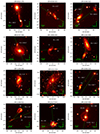 |
Fig. 1. Examples of r′ filter acquisition images obtained with GMOS-S of the interacting pairs and groups. The slits are represented in green, with the nuclear aperture used here shown in blue. The remaining images are shown in Fig. A.1 in Appendix https://zenodo.org/records/12528027. |
The data reduction followed standard procedures, using the GEMINI.GMOS routine of the IRAF package (Tody 1986, 1993), except that no flat field correction was applied to the spectroscopic data presented here. This was due to the strong fringing effects present redward of 750 nm, which severely degraded the quality of the data toward the red. For the large apertures extracted here, this has no measurable effect on the data. To make a fair comparison among the galaxies, we extracted all the spectra in a consistent aperture of 2.2 kpc × 0.5″ (0.5″ ≈ 380 pc at the mean distance of the sample).
The imaging data shown in Fig. 1 correspond to the acquisition images taken just before the spectroscopy to center the objects in the slit. The Sloan r′ filter was used, and reduction was standard, including bias and flat-field corrections.
2.2. The interacting and isolated galaxy samples
The redshift of the interacting galaxies was measured using the IRAF tasks RVIDLINES and XCOR, for emission and absorption line spectra, respectively, and adopting H0 = 75 km s−1 Mpc−1 (Spergel et al. 2007). As in previous works, in order to determine if the galaxies belong to a physical system, we constrained the difference between their radial velocities to be Δvr < 500 km s−1 (Patton et al. 2000; Lin et al. 2008; Ventou et al. 2017). Sixty galaxies were found to be in truly interacting systems (19 pairs and six small groups), although we only have GMOS-S spectra for 59 of them. We do not have a GMOS-S spectrum of AM 2106–624 G1 because the slit was misplaced, but it was confirmed as being a member of the pair with AM 2106–624 G2 thanks to a previous radial velocity estimate (see Table A.2 in Appendix https://zenodo.org/records/12528027). Therefore, the following analysis was carried out using the 59 interacting galaxies with spectra, which we refer to as the interacting (INT) sample hereafter. For them, we measured redshifts in the interval 0.006 ≤ z ≤ 0.097. Figs. 1 and 2 show examples of r′ filter acquisition images and observed optical spectra of confirmed pairs and groups. The remaining 40 galaxies include 22 that are just close in projection, and 18 for which the data either did not allow us to constrain their redshifts or were not available. Table A.2 in Appendix https://zenodo.org/records/12528027 presents the radial velocities for the interacting systems and Table B.1 in Appendix https://zenodo.org/records/12528027 for the noninteracting galaxies, together with information about the sources that could not be either confirmed or discarded as interacting.
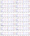 |
Fig. 2. Examples of nuclear rest-frame spectra (2.2 kpc aperture) of the interacting pairs observed with GMOS-S. The main emission lines and absorption features are indicated as vertical red and blue lines, respectively. The remaining spectra are shown in Fig. A.2 in Appendix https://zenodo.org/records/12528027. |
In order to find an adequate control sample of noninteracting galaxies (i.e., isolated sources) comparable in mass and redshift with those of our sample, we first used the broadband magnitudes (JHK) from the Two Micron All Sky Survey (2MASS) extended source catalog (Skrutskie et al. 2006) of the INT galaxies as a proxy for their stellar mass (Davies et al. 2015). We then searched for galaxies with optical spectra in the Sloan Digital Sky Survey (SDSS) III Data Release 9 (DR9, York et al. 2000; Eisenstein et al. 2011; Ahn et al. 2012) matched in redshift and 2MASS JHK magnitudes in the extended source catalog to each of the INT galaxies. The candidates to control sample galaxies for each INT galaxy were then visually inspected using the SDSS images available, and the only ones kept were those that had similar morphologies to the interacting galaxy they matched in infrared magnitude and redshift. In particular, we searched for galaxies of the same galaxy type as each of the INT galaxies (i.e., spirals, lenticulars, or ellipticals) and stellar structures (i.e., bars, rings, and/or spiral arms) and we discarded galaxies with clear signs of interaction and/or close companions of similar mass at distances < 100 kpc.
We note that we selected just one control sample galaxy for each pair member of the INT sample, which is the minimum required for comparison while still being able to analyze the galaxies individually. Fourteen of the interacting galaxies have either too disrupted optical morphologies or do not have infrared magnitudes available in the 2MASS database, and thus no control sample galaxies were selected for them. We did not discard the INT galaxies without controls from the analysis because we checked that the results were consistent including them or not.
Our final control sample of isolated galaxies (CTR sample hereafter) consists of 45 objects, which match the INT sample in redshift, 2MASS J absolute magnitude, and morphology. Figure 3 shows the redshift and absolute J magnitude distribution of the INT and CTR samples. The median, mean, and Kolmogorov–Smirnov (KS) test p-values confirm the similarity between them. Table A.2 in Appendix https://zenodo.org/records/12528027 lists the INT galaxies, radial velocities, and the SDSS DR9 information of the corresponding CTR sample galaxies. The optical spectra of the CTR sample are from SDSS, which uses a 3″ fiber and covers the spectral range 3800−9200 Å, with a spectral resolution (R) varying from R ∼ 1500 at 3800 Å to R ∼ 2500 at 9000 Å. This corresponds to FWHM = 2.78 Å at 7000 Å (Alam et al. 2015; Abolfathi et al. 2018).
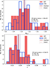 |
Fig. 3. Distribution of absolute magnitudes (using the available extended Jext 2MASS magnitudes) and redshifts for INT (red filled histograms) and CTR (blue continuous line) samples. The plot also shows the samples median, mean values, and their KS test p-values. |
2.3. Stellar population modeling
To perform a stellar population analysis of the galaxies by means of full-spectral fitting of their spectra, we employed the STARLIGHT code (Cid Fernandes et al. 2005; Cid Fernandes 2018). This code combines the spectra of a set of N⋆ simple stellar population (SSP) template spectra denoted as bj, λ. These templates are weighted in varying proportions to replicate the observed spectrum Oλ. The modeling process involves normalizing both the observed and modeled spectra, represented as Mλ, at a user-defined wavelength, λ0. The vector, xj, represents the fractional contribution of the jth SSP to the light at the normalization wavelength, λ0. Additionally, STARLIGHT incorporates a Gaussian distribution, G(v⋆, σ⋆), to address velocity shifts (v⋆) and velocity dispersion (σ⋆). The model spectra can be expressed as
![Mathematical equation: $$ \begin{aligned} M_\lambda = M_{\lambda _0} \left[\sum _{n=1}^{N_\star } x_j\,b_{j,\lambda }\,r_\lambda \right] \otimes G(v_\star , \sigma _\star ), \end{aligned} $$](/articles/aa/full_html/2024/09/aa49360-24/aa49360-24-eq1.gif) (1)
(1)
where Mλ0 represents the flux of the synthetic spectrum at the wavelength, λ0. To account for reddening, it incorporates the term rλ = 10−0.4(Aλ − Aλ0). In the process of fitting, the code searches for the best-fit parameters by minimizing χ2, defined as
![Mathematical equation: $$ \begin{aligned} \chi ^2 = \sum _{\lambda _i}^{\lambda _f} [(O_\lambda - M_\lambda ) \omega _\lambda ]^2, \end{aligned} $$](/articles/aa/full_html/2024/09/aa49360-24/aa49360-24-eq2.gif) (2)
(2)
where ωλ are the weights of each pixel in the fitting (for more details, see Cid Fernandes et al. 2005).
We employed a “base of elements” known as the GM, which is detailed in Cid Fernandes et al. (2013, 2014). This base was constructed using the MILES (Vazdekis et al. 2010) and González Delgado et al. (2005) models and has been updated with the MILES V11 models (Vazdekis et al. 2016). Our selection includes 21 ages (t = 0.001, 0.006, 0.010, 0.014, 0.020, 0.032, 0.056, 0.1, 0.2, 0.316, 0.398, 0.501 0.631, 0.708, 0.794, 0.891, 1.0, 2.0, 5.01, 8.91, and 12.6 Gyr) and four metallicities (Z = 0.19, 0.40, 1.00, and 1.66 Z⊙). Riffel et al. (2021, 2023) and references therein contain more details on the applications of this base.
The normalization flux at λ0 was chosen to be the mean value between 5650 Å and 5750 Å. The reddening law used was that of Cardelli et al. (1989), and the synthesis was performed in the spectral range from 3510 Å to 6930 Å (rest frame). An example of stellar population fitting is shown in Fig. 4 for the galaxy AM 1933–422 B.
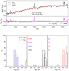 |
Fig. 4. Example of stellar population synthesis of AM 1933–422 B. Top panel: Observed and stellar population synthesis fitting (black and red lines, respectively). The inset at the bottom shows the pure emission line spectra (magenta line). Bottom panel: The left histogram shows, in bins of age, the stellar population contribution in light (solid line) and mass (dashed line) fractions. The middle histogram presents, in bins of age, the metallicity of the fitted stellar populations. The right histogram shows the population vectors in light (solid line) and mass (dashed line) fractions. |
2.4. Emission line fitting
The rest-frame emission-line spectra, free from stellar absorption contribution, have been used to fit the strongest emission lines in the optical region. To this purpose, we used the IFSCUBE1 Python package (Ruschel-Dutra & Dall’Agnol De Oliveira 2020; Ruschel-Dutra et al. 2021). The fitted emission lines are [O II]λλ3726,3729, Hδ, Hγ, [O III]λ4363, Hβ, [O III]λλ4959,5007, He Iλ5876, [O I]λ6300, Hα, [N II]λλ6548,6583, and [S II]λλ6716,6731. The emission-line profiles are fitted with Gaussians by adopting the following constraints: (i) the width and centroid velocities of emission lines from the same parent ion were constrained to the same value; (ii) the centroid velocity was allowed to vary from ±350 km s−1 relative to the velocity obtained from the redshift of each galaxy; (iii) if necessary, a broad component was added in the case of the HI lines to account for the broad line region emission. In addition, we included a first-order polynomial to reproduce the local continuum. We also applied a cut in signal-to-noise (S/N), requiring that the emission line amplitudes be larger than the noise level computed in the line region after the fit in order to have reliable emission line measurements. The emission line flux errors were estimated using the empirical relation described in Lenz & Ayres (1992), Wesson (2016). An example of the emission line fitting is shown in Fig. 5.
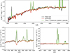 |
Fig. 5. Example of stellar population synthesis and emission line fitting for the galaxy AM 22217–490 G1. The modeled emission lines can be seen as dashed green lines and the stellar synthesis as a red line. The bottom left and right panels correspond to the spectral regions around Hβ and Hα, respectively. |
The extinction correction was made using a Balmer decrement, considering case B for recombination, with Ne = 100 cm−3 and Te = 10 000 K, given an intrinsic ratio of Hα/Hβ = 2.86 (Osterbrock & Ferland 2006) and the extinction law of Cardelli et al. (1989). In summary, the adopted ionized gas optical extinction was computed as Equation (7) of Riffel et al. (2021). The extinction corrected emission lines fluxes for the INT and CTR galaxies are listed in Tables A.3, A.4, A.5, and A.6 in Appendix https://zenodo.org/records/12528027.
3. Stellar populations analysis
Since small differences in the stellar population ages and metallicities are difficult to characterize, to analyze the stellar synthesis output properly, here we used the following binned population vectors (see Cid Fernandes et al. 2005; Riffel et al. 2009, for more details):
Additionally, following Cid Fernandes et al. (2005), we also computed the mean logarithm of the ages and the mean metallicities. The mean logarithm of the ages weighted by the stellar light (hereafter light-weighted mean age) and weighted by the stellar mass (hereafter mass-weighted mean age) are defined as follows:
 (3)
(3)
 (4)
(4)
Furthermore, the light-weighted and mass-weighted mean metallicities are defined as
 (5)
(5)
 (6)
(6)
We note that the definitions above are limited by the ages and metallicities of our stellar population base, as is described in Sect. 2.3.
The results of the stellar population synthesis modeling are summarized in the histograms shown in Fig. 6 and Table 1. In Table 1, besides presenting the mean and median properties of the INT and CTR samples, we also show the fraction of the medians of the INT and CTR sample and the p-values of corresponding KS tests. We reject the null hypothesis that the two samples were drawn from the same distribution if the p-value is < 0.01.
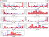 |
Fig. 6. Histograms of the stellar population synthesis modeling for INT (filled red bars) and CTR (full blue lines) samples. The histograms also show the mean (dotted vertical lines) and median (dashed vertical lines) values for both samples and the KS test p-value. The first two rows of histograms present the light-weighted properties. They present the sum of light fractions younger than 2 Gyr (x[y, io] = xy+xiy+xio), the light fractions in the older stellar populations (xo), the light-weighted mean ages, and mean metallicities. The following two rows present the mass-weighted results of the same properties. The lower right histogram shows the stellar extinction of the samples. |
Stellar population synthesis main properties derived for the INT and CTR samples.
The x[y, io]2 and xo histograms in Fig. 6 show a substantial difference between the samples’ stellar populations. The INT galaxies present higher mean and median contributions from x[y, io] than CTR galaxies, as can be also seen in Table 1. This population dominates (x[y, io] > 50%) in more than half of the INT sample (median INT x[y, io] of 55 ± 35%). The INT median contribution of x[y, io] is nearly twice that of the CTR sample (28 ± 18%). On the other hand, 3/4 of the CTR sample galaxies are dominated by the old stellar populations (median CTR xo of 72 ± 18%). Furthermore, the INT light-weighted mean ages have a median value of 1 Gyr younger than the CTR sample (see Table 1 and Fig. 6). These findings suggest that the INT sample has a larger content of stellar populations younger than 2 Gyr than the CTR sample.
These differences between the properties of the stellar populations of the INT and CTR samples are also seen in the mass-weighted properties. Table 1 shows that the INT median, m[y, io]3, is more than three times the CTR, albeit with a large scatter. This result is mainly driven by the intermediate old population (mio), which exhibits an INT median mass fraction contribution nearly five times higher than in the CTR. Consequently, the INT mass-weighted mean ages show a median value 2 Gyr younger than the CTR sample.
The samples also show differences in the mean stellar metallicities of the stellar populations. As is seen in Fig. 6 and Table 1, the light-weighted mean metallicities present similar distributions, with the INT sample presenting a slightly higher median value than the CTR. When considering the mass-weight mean metallicities, the opposite occurs, with the INT median value being smaller than that of the CTR sample. According to the KS test, however, we cannot rule out that they come from the same distribution.
The property that more clearly distinguishes the samples is the stellar extinction ( ). Figure 6 and Table 1 show that the INT sample distribution is shifted toward high
  values compared to the CTR sample. The median INT sample
  is 2.6 times higher than in the CTR. Besides the higher mean and median values, the KS test confirms that the distributions are unlikely to come from the same initial one.
As is seen in Table 1 and Fig. 6, the INT sample often presents much wider distributions, with greater standard and quartile deviations (QDs)4 in stellar populations properties compared to the CTR sample, showing that the INT galaxies span a wider range of stellar population properties. Finally, we did the test of analyzing the stellar population properties by removing the 14 INT galaxies without a CTR (see Sect. 2.2 for more details on the CTR sample selection), and found no significant changes in the overall distributions, median, and mean values.
4. Reddening effects
In the left panel of Fig. 7, we present the  distribution, which is the reddening obtained via the Hα over Hβ emission line flux ratios. As is shown in Table 2, the nebular extinction of the INT sample has higher mean and median values than the CTR. The median ionized gas extinction of the INT sample (median ± Q.D. = 3.0 ± 0.8 mag) is nearly twice the one on the CTR sample (median ± Q.D. = 1.5 ± 0.4 mag). The KS test p-value suggests that the samples are unlikely to come from the same original distribution.
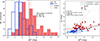 |
Fig. 7. Left panel: Histogram of the gas extinction obtained via Balmer decrement for the INT (in red) and CTR sample galaxies (in blue). The mean and median values of both samples as in Fig. 11. Right panel: Relation between stellar extinction ( |


Ionized gas and stellar extinction properties of the INT and CTR samples.
In the right panel of Fig. 7, we show  vs
vs  plot. The INT sample presents a higher dispersion on both extinctions than the CTR. Consequently, the CTR shows a stronger correlation between the two quantities than the INT galaxies. Some INT galaxies appear to be offset toward high
  and closer to the 1:1 relation. This could suggest that some of these galaxies have a significant fraction of stars in more gas-rich and star-forming regions. This will be further explored in Sect. 7.2.
5. Excitation mechanisms
Emission-line diagnostic diagrams are essential tools used to characterize the main ionization mechanisms of the gas. We applied them to compare the sources of ionization that drive the emission on the INT and CTR samples. Figure 8 presents the traditional BPT diagram (hereafter, [NII] BPT), followed by the diagrams involving [SII]λλ 6717, 6731 Å (hereafter, [SII] BPT), [OI]λ 6300 Å (hereafter, [OI] BPT), and [OII]λλ 3727, 3729 Å (hereafter, [OII] BPT) (Baldwin et al. 1981; Veilleux & Osterbrock 1987). We also used the WHAN diagram (Cid Fernandes et al. 2010, 2011) presented in Fig. 9. In all the diagrams, we plot empirical and theoretical curves (Kewley et al. 2001, 2006; Kauffmann et al. 2003; Stasińska et al. 2006; Cid Fernandes et al. 2011) to enable us to classify the main sources of ionization, which is indicated in Tables A.7 and A.8 in Appendix https://zenodo.org/records/12528027.
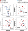 |
Fig. 8. Emission-line diagnostic diagrams used to compare the ionization mechanisms of the INT galaxies (red points) and the CTR sample (blue triangles). Filled symbols correspond to INT (CTR) galaxies whose corresponding CTR (INT) galaxy is also included on that diagram, and open symbols when it is not. Lines in the diagrams represent the theoretical (Kewley et al. 2001) and empirical (Kauffmann et al. 2003; Kewley et al. 2006) divisions applied in this work to classify the ionization sources. Each diagram shows the number of sources included in each diagram. The red cross marks the position on the diagrams of the only type I AGN found in the INT sample. |
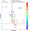 |
Fig. 9. Diagram of [NII]/Hα versus the equivalent width of Hα (WHAN diagram, Cid Fernandes et al. 2010, 2011). INT galaxies are shown as circles, and CTR galaxies are shown as triangles. Symbol colors indicate the light-weighted mean ages of the stellar populations, showing the youngest mean ages in the star-forming galaxies and the oldest in the retired galaxies. Lines represent the divisions applied in this work to obtain the sources of ionization (Stasińska et al. 2006; Kewley et al. 2006; Cid Fernandes et al. 2011). The cross marks the position on the diagram of the only type I AGN found in the INT sample. |
In Fig. 10, we show the histograms with the fractions of activity type classification derived from the diagrams in Figs. 8 and 9. In all diagrams of Fig. 8, the fraction of galaxies for which we could not measure one or more emission lines is higher in the CTR sample. In the BPT diagram, 22% (10/45 sources) of CTR galaxies are not classified, against 15% (9/59 sources) of the INT sample. A similar fraction is found on the [SII] BPT. In the last two diagrams, the absence of classification is higher. The CTR galaxies present a fraction of 49% (22/45 objects) and 62% (28/45 objects) of galaxies unclassified in the [OI] BPT and [OII] BPT, respectively. On the same diagrams, the fraction of INT galaxies that are not classified are 25% in both (15/59 sources).
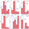 |
Fig. 10. Histograms of the dominant gas ionization mechanisms found from each diagnostic diagram. The three top and the bottom left histograms show the fractions of galaxies classified from the BPT diagrams as SF, AGN (LINER or Seyfert), and composite ([NII] BPT). For the WHAN diagram, the galaxies are classified as retired (RG), SF, strong-AGN (sAGN), and weak-AGN (wAGN). Galaxies that could not be classified in a particular diagram are shown in the histograms as unclassified. The bottom right histogram summarizes the information obtained from all the diagrams, which we divided into four categories: SF, AGN, RG, and inconclusive (INC). Galaxies included in the SF, AGN, and RG groups are those that have the same classification in at least four of the five BPT and WHAN diagrams. |
The WHAN diagram, which includes a higher number of CTR galaxies than the BPTs since several galaxies with Hα equivalent width (EW) < 3 Å may lack the other emission lines involved in the latter, suggests an excess of retired galaxies in the CTR sample, as is seen in Figs. 9 and 10. In this diagram, 33% (15/45 galaxies) of the CTR sources were classified as retired, while in the INT sample the fraction was 22% (13/59 galaxies).
The histograms of Fig. 10 show that more INT galaxies are classified as star-forming than in the CTR. In the BPTs and WHAN diagrams, between 27−59% (16−35/59 galaxies) of the INT sample are classified as star-forming, while in the case of the CTR sample, they represent between 20−55% (9−25/45 sources). The difference is more evident in the [OI] and [OII] BPT diagrams, in which 54% and 63% (32 and 37 out of 59 galaxies) of the INT sample, respectively, are classified as star-forming versus 33% and 31% (15 and 14 out of 45 galaxies) of them in the CTR sample. Our findings suggest that interactions may be responsible for the enhancement in star formation in the INT sample.
When considering the AGN classification in Fig. 10, the Seyfert or strong AGN (sAGN) classification of the INT sources outnumbers the CTR ones in all five diagrams. The diagrams with the highest excess are the [NII] BPT and WHAN, in which the INT sample contains 14−39% (8−23/59 sources) of AGN, respectively, versus 9%−29% (4−13/45 galaxies) of the CTR sample. Although the difference in the fraction of AGN is small, it indicates that nuclear activity might be enhanced due to galaxy interactions in the INT sample.
To find a consensus about the dominant source of ionization of the central region of the INT and CTR galaxies, all five diagrams were combined in the bottom right histogram of Fig. 10. This final classification was done by considering only galaxies with consistent classification in at least four out of the five diagrams. Then, these galaxies were classified into one of the following groups:
-
Star-forming (SF): Galaxies classified as star-forming.
-
Retired galaxies (RGs): Galaxies classified as retired in the WHAN diagram and as LINER in at least three BPT diagrams.
-
AGN: Galaxies classified as LINER, Seyfert, wAGN, sAGN, or composite.
It is important to note that this is a conservative approach since we require the same classification in four out of five diagrams to classify a galaxy as SF, RG, or AGN. The remaining galaxies are classified as inconclusive (INC) in the bottom right histogram of Fig. 10. As can be seen in the first rows of Table 3, we find that 47% (28/59 objects) of the INT sample and 24% (11/45 galaxies) of the CTR sample could be included in each of the three categories listed above. Only one RG was consistently found in the CTR sample. 34% (20/59 sources) of the INT sample and 16% (7/45 objects) of the CTR sample were consistently classified as SF. These results suggest that, even after using our restrictive criteria, there is an excess of 18% of SF galaxies in the INT sample relative to the CTR sample. Regarding the AGN classification, we found that they are more common in the INT sample (8/59 sources, 14%) than in the CTR sample (3/45 sources, 7%).
Classification of the galaxies in the INT and CTR samples using four distinct combinations of diagnostic diagrams.
Relaxing our criteria can reduce the number of galaxies without classification and increase the number of galaxies in both the INT and CTR samples. Table 3 presents the consistent classifications found using three out of the five diagrams (3/5 DGs), [NII] and [SII] BPTs combined with the WHAN diagram ([NII]+[SII]+WHAN), and [NII] BPT with the WHAN diagram ([NII]+WHAN). We were able to find a classification for up to 78% (46/59 galaxies) of the INT sources and 51% (23/45 galaxies) of the CTR sources. We find that the INT sample has between 1.4 to 2.2 times higher fraction of SF galaxies than the CTR sample (0.9 to 1.7 if we exclude the 14 INT galaxies without CTR galaxies). The fraction of AGN in the INT sample is between 2 and 3.4 times greater than the CTR sample (2.3 to 4 if we exclude the 14 INT galaxies without CTR galaxies). Although the fractions change with the criteria and depending on whether we consider INT galaxies with controls or not, we always obtain an excess of AGN galaxies in the INT sample relative to the CTR sample, showing the reliability of this result.
In order to further test how strong the previous results are, we only considered INT galaxies whose CTR is also classified in the same diagram(s). This has the problem that the number of galaxies is then reduced (between four and 19 in the four combinations of diagrams reported in Table 3). By doing this, we measure a fraction of AGN between 1.6 and 2.3 times greater in the INT sample than the CTR sample, confirming the previous result. However, for the fraction of SF the trend reverts, and we find between 1.2 and 1.4 times higher fraction in the CTR sample than in the INT sample. Therefore, based on the analysis done here, we conclude that the number of AGN in the interacting galaxies is larger than in the noninteracting ones, while for the SF galaxies we can neither confirm nor discard any trend.
6. Whether interactions enhance star formation
To evaluate the strength of star formation in both samples, here we consider the INT and CTR sample galaxies classified as SF in the bottom right histogram of Fig. 10 (34% of the INT and 16% of the CTR sample).
The histogram in the left panel of Fig. 11 shows the distribution of EW(Hα) of the SF galaxies and Table 4 summarizes their star formation properties. The SF galaxies in the INT sample have significantly higher EW(Hα) values (median± QD. = 40 ± 28 Å) compared to the SF CTR sample (median± QD. = 19 ± 4 Å). This result suggests the presence of younger stellar populations photoionizing the gas and contributing to this enhancement of EW(Hα) in the INT systems when compared with CTR ones.
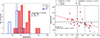 |
Fig. 11. Left panel: Distribution of EW(Hα) for the bona fide SF galaxies. Right panel: Relation between light-weighted mean ages, ⟨t*⟩L, and Hα, equivalent width, for SF galaxies. SF INT galaxies are shown as red circles, and SF CTRs as blue triangles. The dashed red line corresponds to the linear regression fit obtained for the SF INT galaxies. The linear equation, Pearson correlation coefficient (r-value), and p-value of the fit are provided in the inset. The dashed and dotted black lines indicate the mean stellar ages of 100 Myr and 500 Myr, respectively. The dash-dotted line indicates EW(Hα) = 50 Å or log(sSFR/yr−1) = −9.63. |
In the right panel of Fig. 11, we combine the stellar population synthesis modeling results with EW(Hα). Only SF INT galaxies exhibit light-weighted mean stellar ages younger than 100 Myr and EW(Hα) > 50 Å. Furthermore, as is shown in Table 4, the light-weighted mean stellar ages of SF INT galaxies have a median value of 100 Myr, while the SF CTR galaxies exhibit a median value of 1.2 Gyr. The fit of the SF INT galaxies shown in the right panel of Fig. 11 suggests an anti-correlation (Pearson r = −0.48), which is expected if there is a connection between the enhancement of EW(Hα) and the age of the stellar populations.
We can use EW(Hα) to estimate the specific star formation rate, or sSFR (sSFR = SFR/M⋆). Using equation log(sSFR/yr−1) = −11.87 + 1.32 log(EW(Hα)) from Belfiore et al. (2018), we found, as is shown in Table 4, that SF INT galaxies have a median sSFR 2.6 times higher than SF CTR galaxies. At this rate, SF INT galaxies will need less than half of the time of SF CTR galaxies to double their stellar mass. We also calculated the sSFR (see Table 4) from the stellar population modeling, using the SFR20 Myr5, and found similar results as with EW(Hα).
7. Discussion
7.1. The stellar populations and recent star formation of interacting galaxies
It is well known that interactions and mergers can induce star formation (Sanders & Mirabel 1996; Ellison et al. 2013; Knapen et al. 2015; Krabbe et al. 2017). We used stellar population synthesis modeling to confirm or discard the presence of recent star formation in our samples. Our findings reveal that more than half of the INT sample is dominated (see Table 1) by stellar populations younger than 2 Gyr (i.e., higher light-weighted fractions). The median contribution from these young stellar populations in the INT sample is nearly two times that of the CTR sample. This difference between the stellar populations of the INT and CTR samples is also detected in the mass-weighted fractions.
Regarding the stellar populations light-weighted stellar population fractions, our results agree with the findings of previous studies, mostly done in small samples or individual pairs. For instance, Krabbe et al. (2017) analyzed 15 galaxies in nine close pairs using long-slit spectroscopy. They also used STARLIGHT but with BC03 models (Bruzual & Charlot 2003). In agreement with our findings, the stellar population synthesis modeling revealed that 11 out of the 15 galaxies in their sample were dominated in light fractions by young to intermediate stellar populations (< 2 Gyr).
Bessiere et al. (2017) presented optical spectroscopy observations of 21 type-II quasars. Their study investigates the timescales of starburst and AGN triggering associated with merger events. They built stellar population models with STARBURST99 (Leitherer et al. 1999) and fitted the spectra using the routine CONFIT (Robinson et al. 2000). For most quasars, they were able to fit an 8 Gyr plus a young stellar population (YSP). They found YSP light fractions between 15%−100% and maximum YSP ages below 200 Myr. These fractions are much greater than the median values found in our INT sample for our youngest stellar populations. Despite the different models and fitting procedures, most of their quasars are in a later stage in the merging process, and have larger gas masses, both having an impact on star formation.
We also analyzed the star formation enhancement using nebular indicators. Since the Hα equivalent width is a stellar age indicator in HII regions (Copetti et al. 1986; Kennicutt 1998; Kennicutt & Evans 2012; Tacconi et al. 2020; Sánchez 2020; Sánchez et al. 2021) and it is used as a proxy to derive the sSFR, we used it to compare the bona fide SF galaxies in our INT and CTR samples. As is shown in Table 4, the median EW(Hα) for SF INT galaxies is two times higher than for the CTR sample. Higher equivalent widths in interacting systems were also found in Donzelli & Pastoriza (1997). The authors analyzed the spectra of 27 galaxies in pairs and found mean values of the equivalent width of Hα+[NII] ranging from 37−54 Å against a mean of 27 Å in visual pairs (i.e., discarded as pairs spectroscopically).
From EW(Hα) we measure a median sSFR of the SF INT galaxies 2.6 times higher than that of the SF CTR galaxies, which means that at this star formation rate, SF INT galaxies will need less than half of the time of SF CTR galaxies to double their stellar mass. The sSFRs values obtained here are compatible with the ones found in interacting gas-rich spiral galaxies in Knapen et al. (2015). In that work, the authors analyzed 1500 nearby interacting galaxies using estimates of SFR and sSFR from Querejeta et al. (2015) based on far-infrared emission and selected a control sample of isolated galaxies with similar masses and morphologies. They found that the interacting galaxies have SFRs and sSFRs up to twice higher than those measured for the control sample. Hwang et al. (2011) also studied the sSFR in interacting galaxies and found an enhancement in spiral pairs. They found the sSFR to be 1.8 up to 4.0 times higher than in noninteracting galaxies. Their sSFRs are similar to the ones from our work.
7.2. Stellar and nebular reddening.
The analysis of the stellar and ionized gas extinction revealed that the INT sample presents higher median stellar and ionized gas reddening (1.3 ± 0.4 mag and 3 ± 1 mag) than the CTR sample (0.5 ± 0.2 mag and 1.5 ± 0.4 mag, see Tables 1 and 2). These results are in agreement with the previous ones that found that the line-emitting gas is in dustier regions than the stars (Calzetti et al. 1994; Asari et al. 2007; Riffel et al. 2008, 2009, 2021; Riffel et al. 2023; Martins et al. 2013; Dametto et al. 2014; Krabbe et al. 2017).
Calzetti et al. (1994) interpreted this result as due to the fact that the ionized gas is more often associated with dust than the old stellar populations that largely contribute to the stellar continuum. The extinction ratios (see Table 2) are consistent with those reported in the literature for SF (Calzetti et al. 1994; Asari et al. 2007; Riffel et al. 2008) and AGN (Riffel et al. 2021) galaxies, which often report nebular extinctions around twice the stellar. The same was found in interacting pairs (Krabbe et al. 2017).
The interacting galaxies in our sample exhibit higher median stellar and emission-line gas reddening relative to control galaxies. This result suggests that the interacting galaxies are more frequently dustier. This result agrees with Yuan et al. (2012), who found that interacting galaxies, especially spiral pairs, present higher dust attenuation than isolated galaxies using ultraviolet data from GALEX and infrared data from Spitzer (see also Hwang et al. 2011). This is also predicted from simulations (e.g., Yutani et al. 2022) in which an increase of dust in the central regions of interacting galaxies could, in the late stages of the merging process, lead to dust-obscured galaxies (DOGs).
Some interacting galaxies in our sample were found closer to the  =
=  relation shown in Fig. 7 than others. This could indicate that the stellar populations there are associated with dusty SF regions. To confirm this hypothesis, in Fig. 12 we show the relation between the stellar and emission line extinctions in the INT sample, with colors indicating the light-weighted mean ages. The interacting galaxies above the linear fit have median light-weighted mean age of 220 ± 870 Myr (the median value is 3.1 ± 2.3 Gyr in the INT galaxies below the linear fit) meaning that they have a high amount of very hot massive stars. We checked if the distance between the points in Fig. 12 and the 1:1 relation correlates with their light-weighted mean stellar ages, but we did not find any correlation.
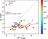 |
Fig. 12. Relation between |


7.3. Triggering of nuclear activity and star formation in interacting galaxies
In our analysis of the main sources of ionization, five different diagnostic diagrams were applied (see Sect. 5). We combine the results of the five diagnostics and require agreement in their classification on at least four diagrams for the sources to be classified as SF, RG, and AGN. Because of the lack of information in some diagnostics, combined with the inconsistencies between the classifications, it was not possible to classify the dominant ionization mechanism for 34 galaxies (76%) in the CTR sample and 31 galaxies (53%) in the INT sample. Considering the galaxies that we could classify, we measure 34% of SF, 14% of AGN, and 0% RGs in the INT sample and 16% of SF, 7% of AGN, and 2% of RGs in the CTR sample.
There are similar works in the literature addressing the classification of galaxies in terms of the dominant ionizing source using optical diagnostic diagrams using large survey data, such as the SDSS-III (York et al. 2000; Eisenstein et al. 2011) and the SDSS-IV integral field spectroscopy (hereafter IFS) survey of Mapping Nearby Galaxies at Apache Point Observatory (MaNGA, Bundy et al. 2015). It is not straightforward to compare with these works since they differ in sample and control sample selection, pair mass ratio and mergers stages, redshifts and analysis methods. Nevertheless, in the next paragraphs, we try to compare our findings with some studies.
Sabater et al. (2013) studied the dependence of the dominant ionizing source of the gas on the environment and interactions using single fiber observations of a sample of 270 000 galaxies from SDSS-III. The authors used the traditional [NII] BPT diagram to classify their sources and applied a cut on [OIII] luminosity to classify the passive galaxies. They found that the incidence of galaxy interactions decreases from SF galaxies to Seyferts to LINERs to passive galaxies.
Ellison et al. (2013) presented a study of 10 800 close pairs and 97 post-mergers using single fiber observations from the SDSS-III. A control sample of isolated galaxies was selected, taking control of the redshift, mass, and density of the environment. As in the previous case, the study used the [NII] BPT diagram, considering as AGN just Seyfert and composite galaxies. They found fractions of SF galaxies of 20% in close pairs (8% in the controls) and 40% in post-merger stages (14% in their controls). They calculated the ratio between the fractions found in the two samples and found that their interacting galaxies present a factor ∼2−3 higher in SF galaxies relative to their controls. The authors also found an increasing AGN excess with decreasing pair separation, presenting a fraction of 2.5 times more AGN in close pairs and 3.75 in post-mergers relative to the control galaxies.
Jin et al. (2021) selected a sample of 1156 galaxies in pairs and 2317 isolated galaxies from the SDSS-IV MaNGA survey. They separated the interacting galaxies in different stages of the merging process and used the [NII] and [SII] BPTs. They used the WHAN diagram only for removing the RGs from their samples. Galaxies were classified as AGN if they fell in the Seyfert or LINER regions of either of the BPT diagrams. They reported 5.5% of AGN, 6.6% of composite galaxies, 27.8% of SF, 28.1% of RGs, and 32% of lineless galaxies in the sample of pairs. For the controls, they find 5% of AGN, 10.2% of composite galaxies, 42.3% of SF, 26.7% of RG and 15.8% of lineless galaxies. The authors argue that they found no significant AGN excess in the pairs compared to the controls. In close pairs in strong interactions, however, they reported a fraction of 19.5% (AGN + composite) against 15.2% in the isolated sample.
Steffen et al. (2023) used the last SDSS-IV MaNGA data release and found 391 pairs (213 minor and 178 major mergers). The control sample was built from 7811 MaNGA galaxies without companions with Δv < 2000 km/s. The dominant ionization source was classified based on the [NII] BPT and on the WHAN diagram to remove the RGs but with a more restricted cutoff in EW(Hα) of 6 Å. The galaxy pairs exhibit 13.4% of AGN (62 composites, 18 LINERs, and 25 Seyferts) versus 11.1% in their control sample (613 composites, 70 LINERs, 126 Seyferts, and 63 broad line AGN).
In our work, we find that the INT sample has between 1.4 and 2.2 times higher fraction of SF galaxies than the controls, depending on the diagnostic diagrams used to classify the galaxies as SF (see Sect. 5). These fractions are compatible with those reported by Ellison et al. (2013). However, this excess of SF galaxies in the INT sample decreases when we exclude the 14 INT galaxies without controls (fractions from 0.9 to 1.7) and it becomes a deficit if we only consider INT (CTR) galaxies with having their twin CTR (INT) galaxy classified in the same diagram (between 1.2 and 1.4 times higher fractions of SF galaxies in the CTR than in the INT sample).
Considering the bona fide AGN that we classified here (including LINER/wAGN, Seyfert/sAGN and Composite galaxies), we find a fraction of 14% (8/59 objects). This is similar to the fractions reported in the works by Jin et al. (2021) (AGN + transition galaxies: 12%) and Steffen et al. (2023) (13%). Using different diagnostic diagrams (BPTs and WHAN) we find between 2 and 3.4 times more AGN in the INT sample than in the CTR sample, which agrees with the factor of 2.5 reported by Ellison et al. (2013) for close pairs. Even when we restrict the sample to include 1) only INT galaxies with CTR and 2) INT (CTR) galaxies having their twin CTR (INT) galaxy classified in the same diagram, we still find a higher fraction of AGN in the INT sample relative to the CTR sample, ranging from 1.6 to 4.
7.4. Interacting pairs’ properties
Many studies found younger stellar populations in the smaller member of galaxy pairs (e.g., Krabbe et al. 2008, 2011; Alonso-Herrero et al. 2012). In order to check if this is also the case for our INT pairs, we calculated their mass ratios using the stellar masses obtained from the stellar population modeling and selected the ones in which one of the galaxies is more than twice the mass of the other (M*A > 2M*B). We found that 11 of the 18 pairs with spectra satisfy this criterion. Figure 13 shows the sum of light and mass fractions younger than 2 Gyr (x[y, io] and m[y, io]) and the light- and mass-weighted mean stellar ages (⟨t⋆⟩L and ⟨t⋆⟩M) of the A and B members of the pairs. We find that the least massive galaxies in the pairs (B) have a median x[y, io] = 84 ± 26% and ⟨t⋆⟩L = 8.7 ± 0.5, while the most massive (A) have x[y, io] = 54 ± 35% and ⟨t⋆⟩L = 9.1 ± 0.7. In mass fractions, for the B galaxies in the pairs we measure a median m[y, io] = 53 ± 40% and ⟨t⋆⟩M = 9.5 ± 0.4, and for the A galaxies a median m[y, io] = 11 ± 32% and ⟨t⋆⟩M = 9.9 ± 0.3. Therefore, we find a higher fraction of young stellar populations (ages ≤2 Gyr) in the least massive galaxies of galaxy pairs with M*A > 2M*B, although we cannot ensure that the distributions are different based on the KS-test p-values that we find (see Fig. 13).
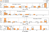 |
Fig. 13. Histograms of the light and mass fractions younger than 2 Gyr (x[y, io] and m[y, io]) and light- and mass-weighted mean stellar ages (⟨t⋆⟩L and ⟨t⋆⟩M) of the A (filled histograms) and B members (empty histograms) of INT pairs with M[A]> 2M[B]. The histograms also show the mean (dotted vertical lines), median (dashed vertical lines), and KS p-values. |
Several publications also reported that both star formation and nuclear activity are enhanced with decreasing pair separation (e.g., Ellison et al. 2013; Satyapal et al. 2014; Steffen et al. 2023). Therefore we measured the projected separation between the two members of the 18 pairs using the r′ band acquisition images (see Figs. 1 and A.1 in Appendix https://zenodo.org/records/12528027) and looked for possible trends in light- and mass-weighted stellar ages, SFRs, and/or the different BPT and WHAN diagrams considered in previous sections. Although in the case of our pairs we do not find any trend with projected distance between the pair members, we believe that this is due to the narrow range that they span, between 10 and 90 kpc, with 32 out of the 36 galaxies having projected separations ≤40 kpc (i.e., close pairs; Ellison et al. 2013).
8. Summary and conclusions
In this work, we have analyzed spectroscopic observations of 95 galaxies from a parent sample of 100 galaxies in 43 interacting system candidates from the Arp & Madore (1987) catalog. The selected galaxies are pairs and small groups. Most of them had no previous spectroscopic data.
We have found that 60 galaxies are in real interacting systems, mainly in galaxy pairs and groups. A control sample of isolated galaxies was built using SDSS spectra of galaxies matched in redshift, absolute J magnitude, and galaxy morphology to the INT sample. We compared the stellar populations and ionized gas properties of the two samples, INT and CTR, and have found the following.
-
More than half of the INT sample is dominated in light fractions by stellar populations younger than 2 Gyr. Interacting galaxies present a median fraction of these young stellar populations of 55%, compared to 28% found in the CTR sample. This difference is also found in mass fractions: 10% in the INT sample versus 3% in the CTR sample.
-
We find higher stellar and nebular extinction in the interacting galaxies relative to the control sample. The median
 and
and  of the INT sample are 2 and 2.6 times the ones found in the control sample. This suggests that our interacting galaxies are dustier.
 -
We find
 in both the INT and CTR samples, although some INT galaxies have
  . These galaxies are the ones that have the youngest stellar populations in the INT sample, which could explain their high
  values.
 -
We find an excess of AGN in the INT sample relative to the CTR sample. Depending on the diagnostic diagrams employed and the number of INT and CTR sample galaxies considered, the fraction of AGN in the INT sample relative to the CTR sample ranges between 1.6 and 4.
-
Considering the galaxy pairs in the INT sample having M*A > 2 × M*B, we find that the least massive galaxies in the pairs present higher fractions of stellar populations younger than 2 Gyr than the most massive galaxies.
Our study provides further observational evidence that interactions enhance star formation and nuclear activity in galaxies, and therefore can have a significant impact on galaxy evolution.
Data availability
Appendices A and B can be found in the Zenodo repository https://zenodo.org/records/12528027
x[y, io] = xy + xiy + xio. The x[y, io] is the sum of light-fraction contributions of stellar populations younger than 2 Gyr.
m[y, io] = my + miy + mio. The m[y, io] is the sum of mass-fraction contributions of stellar populations younger than 2 Gyr.
The QD is defined as half of the interquartile range (IQR), used as a measure of the dispersion for median values (Kenney 1939).
The star formation rate over the last 20 Myr (SFR20 Myr) was calculated following Riffel et al. (2021, 2023).
Acknowledgments
PHC and CRA acknowledge support from project “Tracking active galactic nuclei feedback from parsec to kiloparsec scales”, with reference PID2022-141105NB-I00. PHC thanks to Conselho Nacional de Desenvolvimento Científico e Tecnológico (CNPq). RR acknowledges support from the Fundación Jesús Serra and the Instituto de Astrofísica de Canarias under the Visiting Researcher Programme 2023-2025 agreed between both institutions. RR, also acknowledges support from the ACIISI, Consejería de Economía, Conocimiento y Empleo del Gobierno de Canarias and the European Regional Development Fund (ERDF) under grant with reference ProID2021010079, and the support through the RAVET project by the grant PID2019-107427GB-C32 from the Spanish Ministry of Science, Innovation and Universities MCIU. This work has also been supported through the IAC project TRACES, which is partially supported through the state budget and the regional budget of the Consejería de Economía, Industria, Comercio y Conocimiento of the Canary Islands Autonomous Community. RR also thanks to Conselho Nacional de Desenvolvimento Científico e Tecnológico (CNPq, Proj. 311223/2020-6, 304927/2017-1, 400352/2016-8, and 404238/2021-1), Fundação de amparo à pesquisa do Rio Grande do Sul (FAPERGS, Proj. 16/2551-0000251-7 and 19/1750-2), Coordenação de Aperfeiçoamento de Pessoal de Nível Superior (CAPES, Proj. 0001). ACK thanks Fundação de Amparo á Pesquisa do Estado de São Paulo (FAPESP) for the support grant 2020/16416-5 and the Conselho Nacional de Desenvolvimento Científico e Tecnológico (CNPq). The authors thank Jose Andres Hernandez Jimenez for helpful discussions. The authors thank the anonymous referee for useful and constructive suggestions.
References
- Abolfathi, B., Aguado, D. S., Aguilar, G., et al. 2018, ApJS, 235, 42 [NASA ADS] [CrossRef] [Google Scholar]
- Ahn, C. P., Alexandroff, R., Allende Prieto, C., et al. 2012, ApJS, 203, 21 [Google Scholar]
- Alam, S., Albareti, F. D., Allende Prieto, C., et al. 2015, ApJS, 219, 12 [Google Scholar]
- Alonso-Herrero, A., Rosales-Ortega, F. F., Sánchez, S. F., et al. 2012, MNRAS, 425, L46 [CrossRef] [Google Scholar]
- Araujo, B. L. C., Storchi-Bergmann, T., Rembold, S. B., Kaipper, A. L. P., & Dall’Agnol de Oliveira, B. 2023, MNRAS, 522, 5165 [NASA ADS] [CrossRef] [Google Scholar]
- Argudo-Fernández, M., Yuan, F., Shen, S., et al. 2015, Galaxies, 3, 156 [CrossRef] [Google Scholar]
- Argudo-Fernández, M., Shen, S., Sabater, J., et al. 2016, A&A, 592, A30 [NASA ADS] [CrossRef] [EDP Sciences] [Google Scholar]
- Arp, H. C., & Madore, B. 1987, A Catalogue of Southern Peculiar Galaxies and Associations (Cambridge: Cambridge University Press) [Google Scholar]
- Asari, N. V., Cid Fernandes, R., Stasińska, G., et al. 2007, MNRAS, 381, 263 [Google Scholar]
- Azevedo, G. M., Chies-Santos, A. L., Riffel, R., et al. 2023, MNRAS, 523, 4680 [NASA ADS] [CrossRef] [Google Scholar]
- Baldwin, J. A., Phillips, M. M., & Terlevich, R. 1981, PASP, 93, 5 [Google Scholar]
- Belfiore, F., Maiolino, R., Bundy, K., et al. 2018, MNRAS, 477, 3014 [Google Scholar]
- Bessiere, P. S., Tadhunter, C. N., Ramos Almeida, C., & Villar Martín, M. 2012, MNRAS, 426, 276 [NASA ADS] [CrossRef] [Google Scholar]
- Bessiere, P. S., Tadhunter, C. N., Ramos Almeida, C., & Villar Martín, M. 2014, MNRAS, 438, 1839 [NASA ADS] [CrossRef] [Google Scholar]
- Bessiere, P. S., Tadhunter, C. N., Ramos Almeida, C., Villar Martín, M., & Cabrera-Lavers, A. 2017, MNRAS, 466, 3887 [NASA ADS] [CrossRef] [Google Scholar]
- Böhm, A., Wisotzki, L., Bell, E. F., et al. 2013, A&A, 549, A46 [NASA ADS] [CrossRef] [EDP Sciences] [Google Scholar]
- Bruzual, G., & Charlot, S. 2003, MNRAS, 344, 1000 [NASA ADS] [CrossRef] [Google Scholar]
- Bundy, K., Bershady, M. A., Law, D. R., et al. 2015, ApJ, 798, 7 [Google Scholar]
- Calzetti, D., Kinney, A. L., & Storchi-Bergmann, T. 1994, ApJ, 429, 582 [Google Scholar]
- Cardelli, J. A., Clayton, G. C., & Mathis, J. S. 1989, ApJ, 345, 245 [Google Scholar]
- Cid Fernandes, R. 2018, MNRAS, 480, 4480 [NASA ADS] [CrossRef] [Google Scholar]
- Cid Fernandes, R., Mateus, A., Sodré, L., Stasińska, G., & Gomes, J. M. 2005, MNRAS, 358, 363 [Google Scholar]
- Cid Fernandes, R., Stasińska, G., Schlickmann, M. S., et al. 2010, MNRAS, 403, 1036 [Google Scholar]
- Cid Fernandes, R., Stasińska, G., Mateus, A., & Vale Asari, N. 2011, MNRAS, 413, 1687 [Google Scholar]
- Cid Fernandes, R., Pérez, E., García Benito, R., et al. 2013, A&A, 557, A86 [NASA ADS] [CrossRef] [EDP Sciences] [Google Scholar]
- Cid Fernandes, R., González Delgado, R. M., García Benito, R., et al. 2014, A&A, 561, A130 [NASA ADS] [CrossRef] [EDP Sciences] [Google Scholar]
- Cisternas, M., Jahnke, K., Inskip, K. J., et al. 2011, ApJ, 726, 57 [NASA ADS] [CrossRef] [Google Scholar]
- Copetti, M. V. F., Pastoriza, M. G., & Dottori, H. A. 1986, A&A, 156, 111 [NASA ADS] [Google Scholar]
- Cortijo-Ferrero, C., González Delgado, R. M., Pérez, E., et al. 2017a, A&A, 606, A95 [NASA ADS] [CrossRef] [EDP Sciences] [Google Scholar]
- Cortijo-Ferrero, C., González Delgado, R. M., Pérez, E., et al. 2017b, A&A, 607, A70 [NASA ADS] [CrossRef] [EDP Sciences] [Google Scholar]
- Dametto, N. Z., Riffel, R., Pastoriza, M. G., et al. 2014, MNRAS, 443, 1754 [Google Scholar]
- Davies, R. I., Burtscher, L., Rosario, D., et al. 2015, ApJ, 806, 127 [Google Scholar]
- Donzelli, C. J., & Pastoriza, M. G. 1997, ApJS, 111, 181 [NASA ADS] [CrossRef] [Google Scholar]
- Eisenstein, D. J., Weinberg, D. H., Agol, E., et al. 2011, AJ, 142, 72 [Google Scholar]
- Ellison, S. L., Patton, D. R., Mendel, J. T., & Scudder, J. M. 2011, MNRAS, 418, 2043 [NASA ADS] [CrossRef] [Google Scholar]
- Ellison, S. L., Mendel, J. T., Patton, D. R., & Scudder, J. M. 2013, MNRAS, 435, 3627 [CrossRef] [Google Scholar]
- Ellison, S. L., Viswanathan, A., Patton, D. R., et al. 2019, MNRAS, 487, 2491 [NASA ADS] [CrossRef] [Google Scholar]
- Fu, H., Steffen, J. L., Gross, A. C., et al. 2018, ApJ, 856, 93 [NASA ADS] [CrossRef] [Google Scholar]
- Gatti, M., Lamastra, A., Menci, N., Bongiorno, A., & Fiore, F. 2015, A&A, 576, A32 [NASA ADS] [CrossRef] [EDP Sciences] [Google Scholar]
- González Delgado, R. M., Cerviño, M., Martins, L. P., Leitherer, C., & Hauschildt, P. H. 2005, MNRAS, 357, 945 [Google Scholar]
- Heckman, T. M., & Best, P. N. 2014, ARA&A, 52, 589 [Google Scholar]
- Hernández-Toledo, H. M., Cortes-Suárez, E., Vázquez-Mata, J. A., et al. 2023, MNRAS, 523, 4164 [CrossRef] [Google Scholar]
- Hwang, H. S., Elbaz, D., Dickinson, M., et al. 2011, A&A, 535, A60 [NASA ADS] [CrossRef] [EDP Sciences] [Google Scholar]
- Jin, G., Dai, Y. S., Pan, H.-A., et al. 2021, ApJ, 923, 6 [NASA ADS] [CrossRef] [Google Scholar]
- Karouzos, M., Jarvis, M. J., & Bonfield, D. 2014, MNRAS, 439, 861 [NASA ADS] [CrossRef] [Google Scholar]
- Kauffmann, G., Heckman, T. M., Tremonti, C., et al. 2003, MNRAS, 346, 1055 [Google Scholar]
- Kenney, J. F. 1939, Mathematics of Statistics (New York: Van Nostrand) [Google Scholar]
- Kennicutt, R. C. 1998, ARA&A, 36, 189 [NASA ADS] [CrossRef] [Google Scholar]
- Kennicutt, R. C., & Evans, N. J. 2012, ARA&A, 50, 531 [NASA ADS] [CrossRef] [Google Scholar]
- Kewley, L. J., Heisler, C. A., Dopita, M. A., & Lumsden, S. 2001, ApJS, 132, 37 [Google Scholar]
- Kewley, L. J., Groves, B., Kauffmann, G., & Heckman, T. 2006, MNRAS, 372, 961 [Google Scholar]
- Knapen, J. H., Cisternas, M., & Querejeta, M. 2015, MNRAS, 454, 1742 [NASA ADS] [CrossRef] [Google Scholar]
- Koss, M., Mushotzky, R., Veilleux, S., & Winter, L. 2010, ApJ, 716, L125 [Google Scholar]
- Koulouridis, E., Chavushyan, V., Plionis, M., Krongold, Y., & Dultzin-Hacyan, D. 2006, ApJ, 651, 93 [NASA ADS] [CrossRef] [Google Scholar]
- Koulouridis, E., Plionis, M., Chavushyan, V., et al. 2013, A&A, 552, A135 [NASA ADS] [CrossRef] [EDP Sciences] [Google Scholar]
- Krabbe, A. C., Pastoriza, M. G., Winge, C., Rodrigues, I., & Ferreiro, D. L. 2008, MNRAS, 389, 1593 [NASA ADS] [CrossRef] [Google Scholar]
- Krabbe, A. C., Pastoriza, M. G., Winge, C., et al. 2011, MNRAS, 416, 38 [NASA ADS] [Google Scholar]
- Krabbe, A. C., Rosa, D. A., Pastoriza, M. G., et al. 2017, MNRAS, 467, 27 [NASA ADS] [CrossRef] [Google Scholar]
- Leitherer, C., Schaerer, D., Goldader, J. D., et al. 1999, ApJS, 123, 3 [Google Scholar]
- Lenz, D. D., & Ayres, T. R. 1992, PASP, 104, 1104 [NASA ADS] [CrossRef] [Google Scholar]
- Li, W., Nair, P., Irwin, J., et al. 2023, ApJ, 944, 168 [NASA ADS] [CrossRef] [Google Scholar]
- Lin, L., Patton, D. R., Koo, D. C., et al. 2008, ApJ, 681, 232 [Google Scholar]
- Lonsdale, C. J., Persson, S. E., & Matthews, K. 1984, ApJ, 287, 95 [CrossRef] [Google Scholar]
- Marian, V., Jahnke, K., Mechtley, M., et al. 2019, ApJ, 882, 141 [CrossRef] [Google Scholar]
- Martins, L. P., Rodríguez-Ardila, A., Diniz, S., Riffel, R., & de Souza, R. 2013, MNRAS, 435, 2861 [NASA ADS] [CrossRef] [Google Scholar]
- McAlpine, S., Harrison, C. M., Rosario, D. J., et al. 2020, MNRAS, 494, 5713 [NASA ADS] [CrossRef] [Google Scholar]
- Neistein, E., & Netzer, H. 2014, MNRAS, 437, 3373 [Google Scholar]
- Osterbrock, D. E., & Ferland, G. J. 2006, Astrophysics of Gaseous Nebulae and Active Galactic Nuclei (Sausalito: University Science Books) [Google Scholar]
- Pan, H.-A., Lin, L., Hsieh, B.-C., et al. 2019, ApJ, 881, 119 [NASA ADS] [Google Scholar]
- Pastoriza, M. G., Donzelli, C. J., & Bonatto, C. 1999, A&A, 347, 55 [NASA ADS] [Google Scholar]
- Patton, D. R., Carlberg, R. G., Marzke, R. O., et al. 2000, ApJ, 536, 153 [NASA ADS] [CrossRef] [Google Scholar]
- Pierce, J. C. S., Tadhunter, C. N., Gordon, Y., et al. 2022, MNRAS, 510, 1163 [Google Scholar]
- Pierce, J. C. S., Tadhunter, C., Ramos Almeida, C., et al. 2023, MNRAS, 522, 1736 [NASA ADS] [CrossRef] [Google Scholar]
- Querejeta, M., Meidt, S. E., Schinnerer, E., et al. 2015, ApJS, 219, 5 [NASA ADS] [CrossRef] [Google Scholar]
- Raimundo, S. I., Malkan, M., & Vestergaard, M. 2023, Nat. Astron., 7, 463 [NASA ADS] [CrossRef] [Google Scholar]
- Ramos Almeida, C., Tadhunter, C. N., Inskip, K. J., et al. 2011, MNRAS, 410, 1550 [NASA ADS] [Google Scholar]
- Ramos Almeida, C., Bessiere, P. S., Tadhunter, C. N., et al. 2012, MNRAS, 419, 687 [NASA ADS] [CrossRef] [Google Scholar]
- Rembold, S. B., Riffel, R., Riffel, R. A., et al. 2024, MNRAS, 527, 6722 [Google Scholar]
- Riffel, R., Pastoriza, M. G., Rodríguez-Ardila, A., & Maraston, C. 2008, MNRAS, 388, 803 [NASA ADS] [CrossRef] [Google Scholar]
- Riffel, R., Pastoriza, M. G., Rodríguez-Ardila, A., & Bonatto, C. 2009, MNRAS, 400, 273 [Google Scholar]
- Riffel, R., Mallmann, N. D., Ilha, G. S., et al. 2021, MNRAS, 501, 4064 [NASA ADS] [CrossRef] [Google Scholar]
- Riffel, R., Mallmann, N. D., Rembold, S. B., et al. 2023, MNRAS, 524, 5640 [NASA ADS] [CrossRef] [Google Scholar]
- Robinson, T. G., Tadhunter, C. N., Axon, D. J., & Robinson, A. 2000, MNRAS, 317, 922 [NASA ADS] [CrossRef] [Google Scholar]
- Rosa, D. A., Milone, A. C., Krabbe, A. C., & Rodrigues, I. 2018, Ap&SS, 363, 131 [NASA ADS] [CrossRef] [Google Scholar]
- Ruschel-Dutra, D., & Dall’Agnol De Oliveira, B. 2020, https://doi.org/10.5281/zenodo.4065550 [Google Scholar]
- Ruschel-Dutra, D., Storchi-Bergmann, T., Schnorr-Müller, A., et al. 2021, MNRAS, 507, 74 [NASA ADS] [CrossRef] [Google Scholar]
- Sabater, J., Best, P. N., & Argudo-Fernández, M. 2013, MNRAS, 430, 638 [Google Scholar]
- Sánchez, S. F. 2020, ARA&A, 58, 99 [Google Scholar]
- Sánchez, S. F., Walcher, C. J., Lopez-Cobá, C., et al. 2021, Rev. Mex. Astron. Astrofis, 57, 3 [Google Scholar]
- Sanders, D. B., & Mirabel, I. F. 1996, ARA&A, 34, 749 [Google Scholar]
- Satyapal, S., Ellison, S. L., McAlpine, W., et al. 2014, MNRAS, 441, 1297 [Google Scholar]
- Silva, A., Marchesini, D., Silverman, J. D., et al. 2021, ApJ, 909, 124 [Google Scholar]
- Silverman, J. D., Kampczyk, P., Jahnke, K., et al. 2011, ApJ, 743, 2 [NASA ADS] [CrossRef] [Google Scholar]
- Skrutskie, M. F., Cutri, R. M., Stiening, R., et al. 2006, AJ, 131, 1163 [NASA ADS] [CrossRef] [Google Scholar]
- Spergel, D. N., Bean, R., Doré, O., et al. 2007, ApJS, 170, 377 [NASA ADS] [CrossRef] [Google Scholar]
- Stasińska, G., Cid Fernandes, R., Mateus, A., Sodré, L., & Asari, N. V. 2006, MNRAS, 371, 972 [Google Scholar]
- Steffen, J. L., Fu, H., Brownstein, J. R., et al. 2023, ApJ, 942, 107 [NASA ADS] [CrossRef] [Google Scholar]
- Steinborn, L. K., Hirschmann, M., Dolag, K., et al. 2018, MNRAS, 481, 341 [NASA ADS] [CrossRef] [Google Scholar]
- Storchi-Bergmann, T., & Schnorr-Müller, A. 2019, Nat. Astron., 3, 48 [Google Scholar]
- Tacconi, L. J., Genzel, R., & Sternberg, A. 2020, ARA&A, 58, 157 [NASA ADS] [CrossRef] [Google Scholar]
- Tody, D. 1986, SPIE Conf. Ser., 627, 733 [Google Scholar]
- Tody, D. 1993, ASP Conf. Ser., 52, 173 [NASA ADS] [Google Scholar]
- Vazdekis, A., Sánchez-Blázquez, P., Falcón-Barroso, J., et al. 2010, MNRAS, 404, 1639 [NASA ADS] [Google Scholar]
- Vazdekis, A., Koleva, M., Ricciardelli, E., Röck, B., & Falcón-Barroso, J. 2016, MNRAS, 463, 3409 [Google Scholar]
- Veilleux, S., & Osterbrock, D. E. 1987, ApJS, 63, 295 [Google Scholar]
- Ventou, E., Contini, T., Bouché, N., et al. 2017, A&A, 608, A9 [NASA ADS] [CrossRef] [EDP Sciences] [Google Scholar]
- Villforth, C. 2023, Open J. Astrophys., 6, 34 [NASA ADS] [CrossRef] [Google Scholar]
- Villforth, C., Hamann, F., Rosario, D. J., et al. 2014, MNRAS, 439, 3342 [NASA ADS] [CrossRef] [Google Scholar]
- Wesson, R. 2016, MNRAS, 456, 3774 [NASA ADS] [CrossRef] [Google Scholar]
- Woods, D. F., & Geller, M. J. 2007, AJ, 134, 527 [NASA ADS] [CrossRef] [Google Scholar]
- York, D. G., Adelman, J., Anderson, J. E., et al. 2000, AJ, 120, 1579 [Google Scholar]
- Yuan, F. T., Takeuchi, T. T., Matsuoka, Y., et al. 2012, A&A, 548, A117 [NASA ADS] [CrossRef] [EDP Sciences] [Google Scholar]
- Yutani, N., Toba, Y., Baba, S., & Wada, K. 2022, ApJ, 936, 118 [NASA ADS] [CrossRef] [Google Scholar]
- Zaragoza-Cardiel, J., Smith, B. J., Rosado, M., et al. 2018, ApJS, 234, 35 [NASA ADS] [CrossRef] [Google Scholar]
All Tables
Stellar population synthesis main properties derived for the INT and CTR samples.
Classification of the galaxies in the INT and CTR samples using four distinct combinations of diagnostic diagrams.
All Figures
|
Fig. 1. Examples of r′ filter acquisition images obtained with GMOS-S of the interacting pairs and groups. The slits are represented in green, with the nuclear aperture used here shown in blue. The remaining images are shown in Fig. A.1 in Appendix https://zenodo.org/records/12528027. |
| In the text | |
|
Fig. 2. Examples of nuclear rest-frame spectra (2.2 kpc aperture) of the interacting pairs observed with GMOS-S. The main emission lines and absorption features are indicated as vertical red and blue lines, respectively. The remaining spectra are shown in Fig. A.2 in Appendix https://zenodo.org/records/12528027. |
| In the text | |
|
Fig. 3. Distribution of absolute magnitudes (using the available extended Jext 2MASS magnitudes) and redshifts for INT (red filled histograms) and CTR (blue continuous line) samples. The plot also shows the samples median, mean values, and their KS test p-values. |
| In the text | |
|
Fig. 4. Example of stellar population synthesis of AM 1933–422 B. Top panel: Observed and stellar population synthesis fitting (black and red lines, respectively). The inset at the bottom shows the pure emission line spectra (magenta line). Bottom panel: The left histogram shows, in bins of age, the stellar population contribution in light (solid line) and mass (dashed line) fractions. The middle histogram presents, in bins of age, the metallicity of the fitted stellar populations. The right histogram shows the population vectors in light (solid line) and mass (dashed line) fractions. |
| In the text | |
|
Fig. 5. Example of stellar population synthesis and emission line fitting for the galaxy AM 22217–490 G1. The modeled emission lines can be seen as dashed green lines and the stellar synthesis as a red line. The bottom left and right panels correspond to the spectral regions around Hβ and Hα, respectively. |
| In the text | |
|
Fig. 6. Histograms of the stellar population synthesis modeling for INT (filled red bars) and CTR (full blue lines) samples. The histograms also show the mean (dotted vertical lines) and median (dashed vertical lines) values for both samples and the KS test p-value. The first two rows of histograms present the light-weighted properties. They present the sum of light fractions younger than 2 Gyr (x[y, io] = xy+xiy+xio), the light fractions in the older stellar populations (xo), the light-weighted mean ages, and mean metallicities. The following two rows present the mass-weighted results of the same properties. The lower right histogram shows the stellar extinction of the samples. |
| In the text | |
|
Fig. 7. Left panel: Histogram of the gas extinction obtained via Balmer decrement for the INT (in red) and CTR sample galaxies (in blue). The mean and median values of both samples as in Fig. 11. Right panel: Relation between stellar extinction ( |
| In the text | |
|
Fig. 8. Emission-line diagnostic diagrams used to compare the ionization mechanisms of the INT galaxies (red points) and the CTR sample (blue triangles). Filled symbols correspond to INT (CTR) galaxies whose corresponding CTR (INT) galaxy is also included on that diagram, and open symbols when it is not. Lines in the diagrams represent the theoretical (Kewley et al. 2001) and empirical (Kauffmann et al. 2003; Kewley et al. 2006) divisions applied in this work to classify the ionization sources. Each diagram shows the number of sources included in each diagram. The red cross marks the position on the diagrams of the only type I AGN found in the INT sample. |
| In the text | |
|
Fig. 9. Diagram of [NII]/Hα versus the equivalent width of Hα (WHAN diagram, Cid Fernandes et al. 2010, 2011). INT galaxies are shown as circles, and CTR galaxies are shown as triangles. Symbol colors indicate the light-weighted mean ages of the stellar populations, showing the youngest mean ages in the star-forming galaxies and the oldest in the retired galaxies. Lines represent the divisions applied in this work to obtain the sources of ionization (Stasińska et al. 2006; Kewley et al. 2006; Cid Fernandes et al. 2011). The cross marks the position on the diagram of the only type I AGN found in the INT sample. |
| In the text | |
|
Fig. 10. Histograms of the dominant gas ionization mechanisms found from each diagnostic diagram. The three top and the bottom left histograms show the fractions of galaxies classified from the BPT diagrams as SF, AGN (LINER or Seyfert), and composite ([NII] BPT). For the WHAN diagram, the galaxies are classified as retired (RG), SF, strong-AGN (sAGN), and weak-AGN (wAGN). Galaxies that could not be classified in a particular diagram are shown in the histograms as unclassified. The bottom right histogram summarizes the information obtained from all the diagrams, which we divided into four categories: SF, AGN, RG, and inconclusive (INC). Galaxies included in the SF, AGN, and RG groups are those that have the same classification in at least four of the five BPT and WHAN diagrams. |
| In the text | |
|
Fig. 11. Left panel: Distribution of EW(Hα) for the bona fide SF galaxies. Right panel: Relation between light-weighted mean ages, ⟨t*⟩L, and Hα, equivalent width, for SF galaxies. SF INT galaxies are shown as red circles, and SF CTRs as blue triangles. The dashed red line corresponds to the linear regression fit obtained for the SF INT galaxies. The linear equation, Pearson correlation coefficient (r-value), and p-value of the fit are provided in the inset. The dashed and dotted black lines indicate the mean stellar ages of 100 Myr and 500 Myr, respectively. The dash-dotted line indicates EW(Hα) = 50 Å or log(sSFR/yr−1) = −9.63. |
| In the text | |
|
Fig. 12. Relation between |
| In the text | |
|
Fig. 13. Histograms of the light and mass fractions younger than 2 Gyr (x[y, io] and m[y, io]) and light- and mass-weighted mean stellar ages (⟨t⋆⟩L and ⟨t⋆⟩M) of the A (filled histograms) and B members (empty histograms) of INT pairs with M[A]> 2M[B]. The histograms also show the mean (dotted vertical lines), median (dashed vertical lines), and KS p-values. |
| In the text | |
Current usage metrics show cumulative count of Article Views (full-text article views including HTML views, PDF and ePub downloads, according to the available data) and Abstracts Views on Vision4Press platform.
Data correspond to usage on the plateform after 2015. The current usage metrics is available 48-96 hours after online publication and is updated daily on week days.
Initial download of the metrics may take a while.