| Issue |
A&A
Volume 685, May 2024
|
|
|---|---|---|
| Article Number | A136 | |
| Number of page(s) | 30 | |
| Section | Planets and planetary systems | |
| DOI | https://doi.org/10.1051/0004-6361/202346380 | |
| Published online | 17 May 2024 | |
Dynamics and potential origins of decimeter-sized particles around comet 67P/Churyumov-Gerasimenko
1
Max Planck Institute for Solar System Research,
Justus-von-Liebig-Weg 3,
37077
Göttingen,
Germany
e-mail: This email address is being protected from spambots. You need JavaScript enabled to view it.
2
Institute for Geophysics and Extraterrestrial Physics, TU Braunschweig,
Mendelssohnstraße 3,
38106
Braunschweig,
Germany
3
CNRS, Laboratoire J.-L. Lagrange,
Observatoire de la Côte d’Azur,
06304
Nice,
France
4
Aurora Technology B.V. for ESA, ESAC,
Madrid,
Spain
Received:
10
March
2023
Accepted:
16
February
2024
Abstract
Context. One of the primary goals of the European Space Agency’s Rosetta mission to comet 67P/Churyumov-Gerasimenko was to investigate the mechanisms responsible for cometary activity.
Aims. Our aim is to learn more about the ejection process of large refractory material by studying the dynamics of decimeter-sized dust particles in the coma of 67P and estimating their potential source regions.
Methods. We algorithmically tracked thousands of individual particles through four OSIRIS/NAC image sequences of 67P’s near-nucleus coma. We then traced concentrated particle groups back to the nucleus surface, and estimated their potential source regions, size distributions, and projected dynamical parameters. Finally, we compared the observed activity to dust coma simulations.
Results. We traced back 409 decimeter-sized particles to four suspected source regions. The regions strongly overlap and are mostly confined to the Khonsu-Atum-Anubis area. The activity may be linked to rugged terrain, and the erosion of fine dust and the ejection of large boulders may be mutually exclusive. Power-law indices fitted to the particle size–frequency distributions range from 3.4 ± 0.3 to 3.8 ± 0.4. Gas drag fits to the radial particle accelerations provide an estimate for the local gas production rates (Qg = 3.6 × 10⁻⁵ kg s−1 m−2), which is several times higher than our model predictions based on purely insolation-driven water ice sublimation. Our observational results and our modeling results both reveal that our particles were likely ejected with substantial nonzero initial velocities of around 0.5–0.6 m s−1.
Conclusions. Our findings strongly suggest that the observed ejection of decimeter-sized particles cannot be explained by water ice sublimation and favorable illumination conditions alone. Instead, the local structures and compositions of the source regions likely play a major role. In line with current ejection models of decimeter-sized particles, we deem an overabundance of CO2 ice and its sublimation to be the most probable driver. In addition, because of the significant initial velocities, we suspect the ejection events to be considerably more energetic than gradual liftoffs.
Key words: comets: general / zodiacal dust / comets: individual: 67P/Churyumov / Gerasimenko
© The Authors 2024
 Open Access article, published by EDP Sciences, under the terms of the Creative Commons Attribution License (https://creativecommons.org/licenses/by/4.0), which permits unrestricted use, distribution, and reproduction in any medium, provided the original work is properly cited.
This article is published in open access under the Subscribe to Open model.
Open Access funding provided by Max Planck Society.
1 Introduction
Comets are small Solar System objects that formed in the outer regions of our protoplanetary disk beyond the snowline (e.g., Weissman et al. 2020). At these heliocentric distances, water and other (super-)volatiles like CO2 can remain solid over astronomical timescales. These ices make up a significant part of cometary material, which otherwise consists mainly of refractory aggregates. Because of this ice content, comets become active once they enter the inner Solar System: their ices start to sublimate. If this happens beneath the cometary surface, the expanding gas can get trapped and build up pressure. Eventually, this pressure may overcome the gravity and tensile strength of the overlying material, expel the gas, and eject some of the refractory material along with it. The released gas and dust then form the characteristic cometary coma, tail, and trail (e.g., Agarwal et al. 2023).
Decimeter-sized particles1 are likely ejected by CO2 ice sublimation in deeper surface layers (e.g., Gundlach et al. 2020; Fulle et al. 2020; Wesołowski et al. 2020; Ciarniello et al. 2022; Davidsson et al. 2022), but the responsible mechanisms are not yet fully understood (e.g., Zakharov et al. 2022; Bischoff et al. 2023; Agarwal et al. 2023, and even less so for small particles where cohesion forces dominate, e.g., Gundlach et al. 2015; Skorov et al. 2017; Markkanen & Agarwal 2020).
Learning more about these processes was, and still is, one of the primary science goals of the European Space Agency’s Rosetta mission to comet 67P/Churyumov–Gerasimenko (e.g., Taylor et al. 2017). The spacecraft rendezvoused with 67P in August 2014 and accompanied the comet through its perihelion passage in August 2015, until Rosetta was set on an intercept course with 67P on September 30, 2016, and landed on its surface. Among the suite of Rosetta’s science instruments was the Optical, Spectroscopic, and Infrared Remote Imaging System (OSIRIS), which consisted of a wide-angle and a narrow-angle camera (WAC and NAC, Keller et al. 2007). During the rendezvous phase, these cameras recorded many image sequences of the near-nucleus coma, which also captured the motion of individual dust particles shortly after their ejection. Because the study of their dynamics can help to understand their ejection process, we developed a particle tracking algorithm for OSIRIS images in Pfeifer et al. (2022).
For the current paper we have now applied an enhanced version of this algorithm to four OSIRIS/NAC image sequences. In Sect. 2 we give an overview of the image sequences. In Sect. 3, we briefly discuss how we improved the tracking algorithm, and explain why we only focus on certain particle groups for our analysis, and how we selected them and identified their suspected source regions. In Sect. 4, we investigate these regions, determine the particle size–frequency distributions, reconstruct the local illumination conditions and surface accelerations, analyze the particle dynamics, and compare the results to dust coma simulations. Finally, in Sect. 5 we summarize our findings and conclusions.
2 Data selection
We chose the four most suitable image sequences for our analysis from a group of about 100 similar sequences. The others were rejected for various reasons (listed in Appendix B), but to summarize, we looked for (preferably complete) image sequences that were recorded in image pairs over a roughly 2-h time span and no farther than ≈ 150 km from the nucleus, and that consist of two subsequences (one short, one long), contain (trackable) sidereal objects, and show at least one concentrated group of high-quality particle tracks.
The four selected sequences were recorded by OSIRIS/NAC between December 16, 2015, and January 6, 2016 (see Table and Keller et al. 2007). They each consist of 44 images and are the result of merging two subsequences (OSIRIS activity tags "JETS_MOVIE" and "DUST_JET"). Figure 1 shows the typical timeline of such a sequence, and Table 2 lists relevant metadata (see also Pfeifer et al. 2022). In the following, we call these sequences according to their designated (Rosetta mission) short-time-planning (STP) numbers: STP087, STP088, STP089, and STP090.
As did Pfeifer et al. (2022), we used images of OSIRIS calibration level 3E (Tubiana et al. 2015, see sample images in Figs. 2 and A.1)2. Images of this level are radiometrically calibrated, corrected for in-field and solar stay-light, geometric distortion, and boresight offset (resampled), and are expressed in radiance units (W m−2 sr−1 nm−1). In preparation for the particle tracking, the images additionally underwent a number of pre-processing steps, where the diffuse coma background was removed, the bright nucleus masked out, and the point-sourcelike particles were detected (Pfeifer et al. 2022). For visual confirmation, we then also stacked the cleaned images using only the maximum value that each pixel assumed over the course of the sequence to create a "master image" (see, e.g., Fig. 2). The identified point source coordinates, on the other hand, are passed on to the tracking algorithm, where they are used to reconstruct the particle trajectories.
3 Particle tracking
3.1 Tracking algorithm
To track the detected particles, we used the algorithm described in Pfeifer et al. (2022, see this reference for definitions of technical terms used in the following), which we improved in three significant ways:
1) Because we found that for some tracks, fitting a second-order polynomial is inadequate, we now also allow fitting of third-order polynomials during the extended tracking phase, but only under the condition that the absolute jerk (i.e., change in acceleration) is lower than a certain user-defined threshold. This condition is necessary because the jerk is very sensitive to inaccurate data points. Thus, high jerk values more likely result from pointing fluctuation that we could not completely correct for or from unrelated detections that were erroneously incorporated into a track, rather than from actual physical forces that acted on the particles. Because the tracks generally have a lot more data points than the polynomials have degrees of freedom, and because their fits yield median adjusted R2 values (a measure for the goodness of fit; e.g., Ezekiel 1930; Fahrmeir et al. 2021) that are extremely close to unity (⪆0.9999), we are confident that we are not overfitting our data. Nevertheless, there are other caveats that come with the choice of polynomial degree, specifically concerning the extrapolation of such fits (see Appendix C). We therefore limit extrapolations to a maximum of 30 minutes.
2) Originally, some detections were rejected during the tracking process, even though they were located close to their track and could be visually confirmed to be part of it. We found that they were rejected because their residual offset was too large with respect to their expected location at the corresponding time, according to the fit. We now calculate the residual offset as the shortest distance to the fit, effectively dropping the timing criterion.
3) The radiance values of particle detections are now more accurate. Instead of integrating only over the member-pixels of a point source that are above a certain radiance threshold, we now integrate over all the (sub)pixels that lie within an ellipse containing most of the source’s signal (see also Bertin & Arnouts 1996; Barbary 2016). During the photometry however, we are deliberately not removing any background signal (e.g., derived from elliptical annuli around the detections), because we already removed the local background in preparation for the detection process, on a scale (16 × 16 px) very similar to typical annuli radii (≈ 11–17px; see also Pfeifer et al. 2022).
Figure 3 shows how fitting third-order polynomials in certain cases, and generally calculating the residual offset as the shortest distance to the fit, improves the particle tracking. In the demonstrated case, fitting a third-order polynomial is even necessary to track the particle at all. If a second-order polynomial were used, the tracking parameters would have to be too lenient, which would result in highly inaccurate velocity and acceleration vectors and thus predictions during tracking, causing the algorithm to go astray.
OSIRIS/NAC specifications.
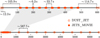 |
Fig. 1 Typical timeline of the four image sequences analyzed, in this case STP089. The other sequences deviate from this structure only by a few seconds at most. |
Metadata of the four sequences analyzed.
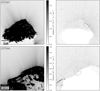 |
Fig. 2 Sample images from sequences STP087 and STP088. First images of the respective sequences on the left, master images on the right. The ellipses in the master images mark the suspected source regions of the concentrated particle groups. All images are brightness-inverted and had their contrasts improved for better readability (for sequences STP089 and STP090 see Fig. A.1). |
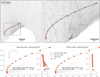 |
Fig. 3 Sample track from sequence STP089 demonstrating how fitting third-order polynomials and calculating the residual as the shortest offset instead of the time-invariant offset can significantly improve the tracking results. Full (brightness-inverted) master image on the top left, close-up on the top right. The sample track is highlighted by the gray arrow, while the orange contours indicate the corresponding point sources. |
3.2 Track selection
In Pfeifer et al. (2022), we introduced a simple but effective criterion–a miss-rate Γ < 30%–to separate genuine from ambiguous tracks, and demonstrated potential applications for our tracking algorithm with tentative first results. While we continue to use the miss-rate criterion as a means of pre-selection, we have now substantially refined the analysis that follows it.
To derive physical properties of ejected particles, such as their sizes and dynamics, it is essential to know the particle-observer distances. Chesley et al. (2020, and references therein), for example, were able to retrieve particle-observer distances and reconstruct the full 3D trajectories of particles around asteroid 101955 Bennu; but doing the same for particles near an active cometary nucleus is extremely difficult. For one, in addition to a complex gravity field, active comets have unknown gaseous environments, whose influence on the particles is complex (Skorov et al. 2016, 2018; Reshetnyk et al. 2018; Ivanovski et al. 2017a,b; Moreno et al. 2022). Secondly, if the (decimeter-sized) particles retain large amounts of water ice after ejection (Gundlach et al. 2020; Davidsson et al. 2021), they may even be outgassing themselves and produce a measurable rocket force (Kelley et al. 2013, 2015; Agarwal et al. 2016; Güttler et al. 2017). Finally, due to the aforementioned residual pointing fluctuation, our positional data is generally not precise enough to account for such effects and reconstruct 3D trajectories. We hence have to work in the 2D image plane and use a different way to approximate the particle-observer distance.
In Pfeifer et al. (2022), we made the basic assumption that particles, whose tracks started close to a central active area on the surface of 67P, and whose velocity vector pointed in the same direction as the estimated surface normal ±45°, likely originated from that area. This allowed us to use the nucleocentric distance as a proxy for the particle-observer distance.
While we still use the nucleocentric distance as an estimate for the particle-observer distance, we now change how the particles for which we make this assumption are selected. First, we find a concentrated group of particles in the master image. Such groups are key, because their tracks intersect the nucleus within a relatively well-defined area. This allows us to assume that the particles (a) were ejected only recently, and (b) share a common origin (two assumptions that are unreasonable to make about the more randomly or homogeneously distributed tracks). Then, we define an ellipse that roughly outlines their suspected source region in the first image of a sequence, placed on the nucleus close to its limb and slightly following its contour (see Fig. 2). Next, we extrapolate the 2D fits of the particle tracks back in time for a maximum of 30 minutes. Within this period, the nucleus rotates at most 14.5°, which results in a displacement of the suspected source region that we still deem acceptable. Lastly, we check whether the tracks intersect with the ellipse within a certain incidence angle range. For those that do, we assume that they likely originated from this area (see Fig. 4). Even though this approach is still relatively simple and some of the selected particles likely originated from somewhere else, in Sec. 4, we show that the general areas are nevertheless plausible.
In the past, it was also suggested that the crossing of particle "streams" can lead to apparent (artificial) features in the particle number/coma density and the average particle motion (and specifically so in the case of coma simulations using fluid dynamics, e.g., Crifo et al. 1995, 2005; Rodionov et al. 2002; Zakharov et al. 2009). More recently, Shi et al. (2018) indeed confirmed that collimated gas and dust flows can result from topographic focusing, but additionally note that apparent jetlike features can also be optical illusions that emerge from projections along the viewing direction. Since we are tracking individual particles however, and thus are not concerned with average coma densities or particle motions within certain volumes along the line of sight, the crossing of particle trajectories is irrelevant in this regard.
During the tracking procedure itself, crossing trajectories are also generally unproblematic. For the tracking algorithm to get confused and jump from one trajectory to the other, they also need to cross at the same time, and have relatively similar speeds, accelerations, and directions. While this can still happen occasionally, such cases are effectively filtered out by our acceptance thresholds and the miss-rate criterion (see Pfeifer et al. 2022). In total, we recovered 11 858 potential particle tracks from the four image sequences, of which 3626 have miss-rates less than 30%. Of those, we traced back 409 to the suspected source regions and visually inspected them several times. We are hence confident that none of the 409 particle tracks that we analyze in the following consist, or were affected by, crossing trajectories. During the entire process, we also did not see any particles colliding or breaking apart.
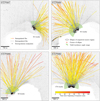 |
Fig. 4 Selected tracks from the four sequences. The fits were extrapolated back in time for a maximum of 30 min. The extrapolated curves end where they are closest to the ellipse centers. The endpoints are hence not intended to mark the exact ejection times or places. |
4 Results and discussion
4.1 Suspected source regions
To get a better idea about where the suspected source regions are located on the nucleus, we used the SPICE toolkit (spacecraft–planet–instrument–c-matrix–events, Acton 1996; ESA SPICE Service 2020) to project the ellipses onto the nucleus surface as it was oriented in the first image of each sequence. For every pixel inside the ellipses, we calculated the points of intersection between the corresponding line of sight and the nucleus shape model SHAP5 (Jorda et al. 2016, in the "cheops" reference frame). Due to 67P’s concave shape however, not every point on its highly irregular nucleus is uniquely identified by the typically-used equidistant cylindrical map projection. Hence, we instead use the recently developed quincuncial adaptive closed Kohonen (QuACK) projection (Grieger 2019; Leon-Dasi et al. 2021) to present our data. Figure 5, for example, shows how the four suspected source regions project onto the south-centered QuACK map.
As already indicated in Sec. 2, we chose the suspected source regions according to which parts in the master images looked to be most active. Because the diffuse coma and jet-like features have mostly been removed in these images, the choices were based on where the largest, concentrated groups of point-source-like particles appeared to originate from. Interestingly, the suspected source regions do not necessarily coincide with the locations of the strongest diffuse features. In other words, it seems that the ejection of large particles (likely of at least a few centimeters) does not always correlate in location, strength, or orientation with that of small (probably subcentimeter) particles (cf. images in Figs. 2 and A.1).
We also observed this seeming anti-correlation in several other sequences not discussed in detail here. In some of those cases, the spacecraft may have been too far away from the nucleus to distinguish even boulders from the diffuse dust features above its surface, and in others, the phenomenon may be explained by the fact that the sequences were recorded during 67P’s perihelion phase, when the comet was most active and dominated by water ice sublimation (e.g., Combi et al. 2020; Läuter et al. 2020), which, according to current activity models, can only eject fine dust particles (≲ 1 cm) due to its shallow sublimation front, while CO2 ice sublimation is responsible for the ejection of larger chunks (e.g., Gundlach et al. 2020; Fulle et al. 2020; Wesołowski et al. 2020; Ciarniello et al. 2022; Davidsson et al. 2022). Yet according to recent thermal modeling by Nicholas Attree (priv. comm.)4, the fine-dust erosion driven by water ice sublimation and the ejection of large particles driven by CO2 ice sublimation cannot happen simultaneously at the same location. The observed lack of large particles within the strong, diffuse dust features may therefore be evidence of this activity-based separation. Notably, Kelley et al. (2013, 2015) already observed the same phenomenon for comet 103P/Hartley 2, but they suspected dynamical processes like the rotation of the nucleus, solar radiation pressure, or rocket forces from asymmetric outgassing to be responsible.
It may also seem as if the nucleus is not homogeneously, but only locally active in this particle size regime. This observation could be biased however due to our selection criteria of the image sequences (cf. Sec. 2), as we were specifically looking for sequences with strong, local activity to fulfill our basic assumptions. Nevertheless, our data clearly show that there are times when inhomogeneous activity occurs.
As illustrated in Fig. 5, all four suspected source regions overlap substantially. While the recorded local time periods of the four sequences are very similar (with the exception of sequence STP087, see Table 3), these areas are not the only ones that were illuminated and visible during the observations (see Figs. 8–10, especially because of the different viewing geometries). We could thus have picked areas that lie much farther apart, had there been stronger activity elsewhere. This indicates that the observed activity was likely locally confined and reoccurring.
It also shows that despite our relatively simple selection process, we likely located the general areas of the source regions correctly. This is further supported by the distinct ejection cones formed by the trajectories that taper toward the ellipse centers (see Fig. 4). To some extent, these ejection cones are likely a consequence of our selection criteria (such as the incidence angle range) and the viewing geometries. Yet their shapes, orientations, and opening angles also suggest that they were likely notably affected by the local surface morphology. Since, to our knowledge, this is the first time such ejection cones have been observed or described, there are currently no theories that explain their occurrence. Their appearance is nevertheless reminiscent of meteorite impacts (e.g., Opik 1936; Arakawa et al. 2017, 2020; Wada et al. 2021), volcanic eruptions (e.g., Tsunematsu et al. 2016; Cigala et al. 2017, 2021; Schmid et al. 2020), cryovolcanism (e.g., Quick et al. 2013; Liu et al. 2016; Fagents et al. 2022), and, of course, cometary jets/geysers/outbursts (e.g., Keller et al. 1987; Wallis & Chandra Wickramasinghe 1992; Yelle et al. 2004; A’Hearn et al. 2011; Lin et al. 2017; Shi et al. 2019; Wesołowski et al. 2020). The relatively slow and decentralized release of dust particles however (i.e., resulting not from a singular responsible event, but rather many small, independent ones), from a rough, cometary terrain into the vacuum of space, seems to be unique.
According to Fig. 5, the selected particles should have been predominantly ejected from the Khonsu, Atum, and Anubis regions, and potentially also from Imhotep and Seth (following the regional definitions of El-Maarry et al. 2015, 2016, 2017b; Thomas et al. 2018). The terrains of these regions are very diverse. Generally, the relatively compact area that is covered by the suspected source regions contains almost every kind of (geomorphological) feature that was observed on the nucleus, be it smooth, or consolidated and outcropped. This includes ridges, terraces, scarps, niches, (coarse or fine grained) dust-blankets, boulders (El-Maarry et al. 2015, 2016; Ferrari et al. 2018; Thomas et al. 2015b, 2018; Leon-Dasi et al. 2021), (steep) cliffs (Attree et al. 2018a), fractures and other linear features (Giacomini et al. 2016; Lee et al. 2016), bright spots (associated with freshly exposed volatiles, Deshapriya et al. 2016, 2018; Fornasier et al. 2023), jet sources (Vincent et al. 2016a; Fornasier et al. 2019; Lai et al. 2019), and potentially even clods or "goosebumps" (Sierks et al. 2015; Davidsson et al. 2016). Khonsu in particular also contains the striking landmark dubbed "pancake feature" (El-Maarry et al. 2016), and has been found to be one of 67P’s most active regions (Deshapriya et al. 2016; Hasselmann et al. 2019).
Due to this variety in morphology, there are several locations within the suspected source regions that could be the origin of the observed activity. In the area near the pancake feature, for example, Vincent et al. (2016a) and Fornasier et al. (2019) located several jet sources, Fornasier et al. (2023) identified many bright spots (see Fig. 5), and Hasselmann et al. (2019) discovered surface changes such as boulder movements and cavity formations. All these occurrences however essentially happened throughout Rosetta’s entire rendezvous phase with 67P, and not specifically during our observational period. Nevertheless, the area near the pancake feature substantially overlaps with the suspected source regions (and even the ellipse centers) of sequences STP087 and STP089, which identifies it as a probable source of the particles associated with these regions.
The suspected source regions of sequences STP088 and STP090, on the other hand, predominantly coincide with Atum and Anubis, which are two vastly different areas. While Atum is an elevated region that mainly consists of consolidated structures like terraces, ridges, and scarps, Anubis is a flat area, which is mostly covered in smooth material, but that also displays some fractures (El-Maarry et al. 2015, 2016; Thomas et al. 2018; Leon-Dasi et al. 2021). Even though these areas have not yet been studied as closely as Khonsu, Fig. 5 shows that especially around the suspected source region of sequence STP088, Vincent et al. (2016a) and Fornasier et al. (2019) have located several jet sources, which might be related to the activity we observed. Additionally, there is a long terrace with a scarp in this area (Lee et al. 2016; Leon-Dasi et al. 2021), so the activity might have also come from an event similar to the cliff collapse discovered at the Aswan site (Pajola et al. 2016c).
In the case of sequence STP090, it is also possible that the activity was caused by retreating scarps of fine material that were reported in this area (El-Maarry et al. 2017a), or by the formation and deepening of fractures (Leon-Dasi et al. 2021), which can facilitate activity (Höfner et al. 2017). STP090’s suspected source region also includes steep cliffs located in Seth (Attree et al. 2018a), but it seems less likely that the observed particles originated from there since the cliffs were not as strongly illuminated during the observational period as the other areas (see Sec. 4.3).
Finally, the suspected source regions not only lie close to where Combi et al. (2020) estimates the four major volatiles (H2O, CO2, CO, and O2) have caused the most erosion between 67P’s inbound equinox and August 2016, but they also notably overlap with two areas that Läuter et al. (2019, 2020, 2022) estimate to be among the most active in water and CO2 production (and possibly many other species) during the perihelion phase, but also long afterward. Figure 6 shows the QuACK-map of the water emission rates predicted by Läuter et al. (2022). The data was averaged over the period between December 13, 2015, and January 14, 2016, which aligns closely with the overarching time frame of our observations. While the suspected source regions of STP087 and STP089 partly overlap with their area 1, the regions of STP088 and STP090 do so with their area 2.
Overall, we can generally associate the ejected particles with areas that contain rugged terrain or steep slopes, be it scarps, cliffs, or fractures. Such geological features are also considered to favor activity, because they (a) should make it easier for particles to overcome the local gravity and tensile strength that keep them in place (Groussin et al. 2015; Attree et al. 2018a,b), (b) can absorb and store energy more efficiently than flat or smooth areas (Höfner et al. 2017), and (c) do not get covered by loose material that could quench their activity (Vincent et al. 2016b). Additionally, we can likely link some of the observed activity to surface areas with a high concentration of jet sources and bright spots, which fits well with our assumptions: Both features indicate (recent) activity, as bright spots may be the remnants of meter-sized, water-ice-enriched blocks (WEBs, Ciarniello et al. 2022) that were exposed due to erosion driven by CO2 ice sublimation.
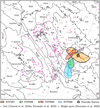 |
Fig. 5 QuACK-map of 67P’s nucleus, centered on its south pole (SP). The colored shapes show how the ellipses that mark the suspected source regions project onto the surface. The lines in the respective colors indicate the projected ellipse centers. For the geographic data such as surface regions (black lines), latitudes (dotted, light gray lines), and longitudes (dashed, gray lines), the publicly available maps provided by Leon-Dasi et al. (2021)3 were used (slightly modified). For the data of the bright spots, see also Oklay et al. (2017); Deshapriya et al. (2018); Hasselmann et al. (2019); Fornasier et al. (2016, 2017). |
Summarized findings regarding the four suspected source regions.
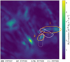 |
Fig. 6 South-centered QuACK-map of the water emission rates predicted by Läuter et al. (2022), averaged over the period between December 13, 2015, and January 14, 2016 (data kindly provided by Matthias Läuter and Tobias Kramer). Also shown are the four suspected source regions and the approximate locations of areas 1 and 2 (orange ellipses, drawn in by hand) from Läuter et al. (2022). |
4.2 Particle size-frequency distribution
Because we associated the particle groups with regions on the nucleus surface, we can use the average nucleocentric distances of the spacecraft (see Table 2) as rough estimates for the particle-observer distances. By further assuming that the particles are spherical, we can approximate their equivalent radii via
![Mathematical equation: $\[r=\sqrt{J \frac{r_{\mathrm{h}}^2 \Delta^2}{R I_{\odot}}},\]$](/articles/aa/full_html/2024/05/aa46380-23/aa46380-23-eq7.png) (1)
(1)
where r is the particle radius in m, J the particle flux averaged over all its detections in Wm−2 nm−1, rh the dimensionless heliocentric distance measured in units of AU, Δ the particle-observer distance in m, R = 0.0021 the particle reflectance (computed for decimeter-sized particles at a 90° phase angle using the model from Markkanen et al. 2018), and I⊚ = 1.565 Wm−2 nm−1 the solar flux in the NAC F22 filter at 1 AU.
For distinct size ranges, it is generally assumed that the size-frequency distribution (SFD) of cometary particles follows a power law. When it comes to particles that are found on the nucleus surface (other than fall-back material), there is good reason to believe that they mostly formed under fractal fragmentation processes like thermal fatigue or gravitational collapse (Pajola et al. 2015, 2017a; Attree et al. 2018b; Cambianica et al. 2019), which have been studied extensively for terrestrial material (e.g., Mandelbrot 1982; Turcotte 1986; Sanchidrián et al. 2014; Fowler & Scheu 2016). Impact and collisional fragmentation, as seen in asteroids for example, also produce fractal SFDs (Dohnanyi 1969; Hartmann 1969; Brown 1989), but likely only play a minor role in the case of 67P (so far, evidence for just a single impact crater has been found, Thomas et al. 2015b).
Numerous studies have determined SFDs of 67P’s surface material and fitted them with power laws (e.g., Auger et al. 2015; Mottola et al. 2015; La Forgia et al. 2015; Pommerol et al. 2015; Vincent et al. 2015, 2016b; Pajola et al. 2015, 2016a,b,c, 2017a,b, 2019; Deshapriya et al. 2016; Poulet et al. 2016; Oklay et al. 2016, 2017; Lucchetti et al. 2016, 2017; Tang et al. 2017; Hasselmann et al. 2019; Cambianica et al. 2019). Likewise, power laws have been used for a long time to fit or model the cometary dust environment (e.g., Finson & Probstein 1968a,b; Fulle 1989; Clark et al. 2004; Ishiguro 2008; Kelley et al. 2008, 2009; Agarwal et al. 2010, 2017; Fulle et al. 2010; Soja et al. 2015; Lai et al. 2016; Marschall et al. 2016, 2017, 2019, 2020b; Markkanen et al. 2018), and more recently to describe the SFDs of particles observed by Deep Impact/EPOXI’s camera system around comet 103P/Hartley 2 (Kelley et al. 2013, 2015), and Rosetta’s dust detectors and camera system around comet 67P (e.g., Rotundi et al. 2015; Merouane et al. 2016, 2017; Hilchenbach et al. 2016; Agarwal et al. 2016, 2017; Fulle et al. 2016; Rinaldi et al. 2017). There is however no proven link between the assumption of a power law and the physical origin of the particle SFD (Marco Fulle, priv. comm.). Instead, the power law is mainly of practical use when fitted to a limited size range, because it allows to easily compare different size regimes, and immediately indicates which size range dominates the cross section and volume (mass) distribution (e.g., Fulle et al. 2010, 2016; Rotundi et al. 2015; Blum et al. 2017). We therefore also use power laws to describe the SFDs of our particles.
Generally, if an SFD follows a power law, it means that the radii were drawn from a probability distribution in the form of
![Mathematical equation: $\[p(r) \propto r^{-b} \text{,}\]$](/articles/aa/full_html/2024/05/aa46380-23/aa46380-23-eq8.png) (2)
(2)
where in our context, the exponent b is often called the (differential) power-law index. A common method to fit a power law to data is to construct a histogram from the data and plot it on a log-log scale with logarithmic bins and counts. In this representation, the data form a straight line with slope −b if the histogram follows a power law, which makes it easy to determine the power-law index via least-squares linear regression, but due to systematic errors (like the arbitrary binning intervals), this approach should generally not be trusted (Clauset et al. 2009).
So instead, we rely on maximum-likelihood estimators (MLEs) and Kolmogorov–Smirnov (KS) tests (see, e.g., Feller 1948 for KS tests, but also Snodgrass et al. 2011, who nevertheless favor least-square regression). To fit our data, we use the Python-package powerlaw (Alstott et al. 2014), which is based on the statistical methods of Klaus et al. (2011) and Clauset et al. (2009, see also Virkar & Clauset 2014). Since our data are drawn from a continuous distribution, Eq. (2) can be written as
![Mathematical equation: $\[p(r)=C r^{-b} \text {,}\]$](/articles/aa/full_html/2024/05/aa46380-23/aa46380-23-eq9.png) (3)
(3)
with normalization constant
![Mathematical equation: $\[C=(b-1) r_{\min }^{b-1},\]$](/articles/aa/full_html/2024/05/aa46380-23/aa46380-23-eq10.png) (4)
(4)
where rmin is the lower fitting bound, which is required because p(r) diverges for r → 0. The MLE of b can then be computed as (Muniruzzaman 1957)
![Mathematical equation: $\[\hat{b}=1+n\left[\sum_{i=1}^n \ln \frac{r_i}{r_{\min }}\right]^{-1},\]$](/articles/aa/full_html/2024/05/aa46380-23/aa46380-23-eq11.png) (5)
(5)
where ri ≥ rmin (i = 1, ..., n) are the measured radii. We additionally used KS tests to find the rmin and ![Mathematical equation: $\[\hat{b}\]$](/articles/aa/full_html/2024/05/aa46380-23/aa46380-23-eq12.png) values that produce the best fits (although in the case of sequence STP089, we slightly restricted the allowed range for rmin due to the small number of data points)5.
values that produce the best fits (although in the case of sequence STP089, we slightly restricted the allowed range for rmin due to the small number of data points)5.
Figure 7 shows the resulting particle SFDs and fitted power laws. The size ranges of the four SFDs largely overlap, covering mostly the decimeter-scale. Only sequence STP090 differs notably from the other three, with its SFD shifted toward smaller radii, peaking below 10 cm, and containing the smallest detected particles at roughly 5 cm. In sequence STP089 on the other hand, we detected the largest particle with an equivalent radius of about 1.15 m. Many particles strongly fluctuate in brightness over the course of their tracks however (in large part likely because they are nonspherical rotators), so their mean-flux-based radii only represent the most likely average values. In contrast, the errors from residual background signals and inaccurate particle-observer distances, as well as the uncertainty in the albedo, are typically much smaller than these fluctuations. Our results therefore remain sufficiently precise, and following the terminology of Pajola et al. (2016b), the particles classify as either pebbles (<25 cm) or boulders (>25 cm).
The values of the fitted power-law indices range from 3.4 ± 0.3 to 3.8 ± 0.4 and are all within each others’ error bars, suggesting that most of the mass is contained in the larger particles. Yet most of the large particles were likely not fast enough to leave the gravitational field of the nucleus (see Figs. 12 and 13 in Sec. 4.4), and should have later fallen back onto its surface. Farther out in the coma, the SFDs in this size range might hence be a little steeper. So far however, there are no other studies that report power-law indices for coma particle SFDs in a similar size range (or time period) to corroborate our findings.
Nevertheless, our index values agree notably well with those obtained for submillimeter-sized particles, despite the likely fundamentally different ejection mechanisms: Fulle et al. (2016) report b ≈ 3.7 for dust particles captured during the perihelion phase, and Merouane et al. (2016) report b = 3.1 ± 0.5 for those captured between perihelion and April 2016 (these are currently the two observational periods that most closely match ours and for which b-values exist).
Regarding surface material, the most relevant b-values were obtained by Deshapriya et al. (2016) and Hasselmann et al. (2019), who counted boulders in the Khonsu region (no studies exist yet for Atum or Anubis). Deshapriya et al. (2016) surveyed the entire region using images recorded pre-perihelion on May 2, 2015, and report b = 4.1 +0.2/-0.3 for boulders ranging from 7 to 40 m, whereas Hasselmann et al. (2019) studied a small patch near the pancake feature in images recorded post-perihelion on June 25, 2016, and report b = 2.6 ± 0.01 for boulders ranging from 1.2 to 10 m. This significant flattening of the particle SFD over the course of the perihelion phase might indicate that most of the smaller boulders were removed from the surveyed area, while most of the larger ones remained or fell back onto it. Since our observations were recorded post-perihelion but well before June 25, 2016, the fact that our power-law indices lie in between those reported by Deshapriya et al. (2016) and Hasselmann et al. (2019) might be a reflection of this particle SFD transition.
Overall, our particles may therefore be a link between the debris studied on 67P’s surface and the particles observed and collected in its coma. Not only do they cover a size range that on the upper end overlaps with that of the typically much larger boulders counted on the nucleus surface, and on the lower end with that of the typically much smaller particles detected farther out in the coma (see also Güttler et al. 2017; Ott et al. 2017; Frattin et al. 2021; Lemos et al. 2023, 2024); but from an evolutionary standpoint, they also sit between the relatively pristine surface material which has not yet been ejected (excluding fallback material), and the more processed material found in the coma and beyond which has escaped the nucleus gravity.
4.3 Illumination and surface acceleration
Because solar irradiation fundamentally drives the activity of comets, we created QuACK-maps that show 67P’s average surface illumination during the time periods when our sequences were recorded, to estimate the insolation that our suspected source regions received. The maps were generated using the same approach as described by Grieger (2019), which accounts for the relative orientation between the solar irradiation vector and the surface normals of the QuACK shape model tiles, as well as self-shadowing effects. Because the QuACK shape model is relatively rough however (160 000 tiles), the resulting illumination maps are somewhat blurred. In reality, small-scale surface parts, such as cliff faces, may receive insolation that is much stronger than the average (Pajola et al. 2017a). Activity from such sites may be significantly enhanced, which our employed model would not reflect, but since we are mainly interested in general areas, the illumination maps are adequate.
Because the four sequences were recorded within less than a month (which corresponds to a change in sub-solar latitude of less than six degrees), the illumination conditions averaged over a whole comet day are almost identical on the respective dates and differ mostly in overall intensity. Figure 8 shows the average daily illumination for sequence STP088, which is a good representation for the entire period as its sub-solar latitude is at the center of the covered value range (see Table 2). Additionally, we created two more illumination maps for each of our sequences. The first set shows the average illumination received solely during the observational periods of the respective sequences (see Fig. 9); but because our particles were likely ejected up to half an hour before the sequences were recorded, and because the activity does not immediately follow the exposure to sunlight as temperature and gas pressure first need to build up, the other set shows the average illumination received over the 2 h (roughly 3 h and 51 min in local time) leading up to the observational periods (see Fig. 10).
According to Fig. 8, the suspected source regions clearly received some of the most sunlight over the course of a full comet day at that time. Conversely, Fig. 9 shows that this was not always the case during the observational periods. Surface areas other than the suspected source regions were illuminated just as, or even more strongly during these periods, but did not show nearly the same levels of activity in our image sequences. Yet if the back-extrapolations of our tracks are approximately correct, most of our particles should have been ejected up to half an hour before the observations started (or possibly even earlier). Figure 10 shows that during the 2 h prior to the observations, the illumination conditions for other areas (such as the neck, the small lobe, or Hapi) were a lot different, while the suspected source regions were already well illuminated. This further supports our choice of their general locations. Yet since we did not observe similar activity from areas that received comparable insolation (during either period), it also suggests that strong illumination is necessary, but not sufficient to explain the observed activity.
We thus also investigated the intensity of the local surface acceleration, aS (i.e., the sum of gravity and centrifugal acceleration). Figure 11 shows two QuACK-maps of aS, once normal to the shape model facets and once in radial direction. In both cases, the average downward accelerations within the suspected source regions are relatively high, which means that they cannot explain the localized release of decimeter-sized particles either. The local surface composition and structure therefore seem to be the most probable causes. For one, activity-enhancing topographies as discussed in Sec. 4.1 may play a role (see also Reshetnyk et al. 2021, 2022; Skorov et al. 2021, 2022a,b, 2023, who use models to explore how structural parameters such as porosity and dust layer thickness can affect the gas production rate), but more importantly, we regard a local overabundance of CO2 ice as the most likely driver of decimeter-sized particle ejection (in line with current ejection models, e.g., Gundlach et al. 2020; Fulle et al. 2020; Wesołowski et al. 2020; Ciarniello et al. 2022; Davidsson et al. 2022).
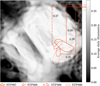 |
Fig. 8 South-centered QuACK-map of the average nucleus illumination received over a whole comet day at the time of sequence STP088 (December 26, 2015). The intensity is measured in units of the average illumination at 1 AU from the Sun at the equator of the Earth over one Earth-day during equinox. The orange shapes and lines indicate the mean values within the suspected source regions. |
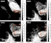 |
Fig. 9 South-centered QuACK-maps of the average surface illumination received during the respective observational periods of the four sequences. The intensity units are the same as in Fig. 8. The mean values within the suspected source regions are indicated by the orange shapes and lines, with the areas that were selected during the respective sequences highlighted in bold. The values here are generally higher than in Fig. 8 because here the illumination was averaged over time periods when the areas were mostly in sunlight, while in Fig. 8 the illumination was averaged over a whole day-and-night cycle. |
4.4 Particle dynamics
From the polynomial fits to the particle tracks we immediately obtain the projected particle velocities and accelerations. Initially, they are measured in terms of the image coordinate system (e.g., in px s−1), so to translate them into physical units, we again need to know the particle-observer distance and thus again use the nucleocentric distance as a proxy (see also Table 2).
Figure 12 shows how the radial components (relative to the nucleus’ center of mass) of the resulting projected particle velocities, υrad, distribute as a function of particle radius, and how they compare to the local escape speed, υesc. Assuming a local surface acceleration at the suspected source regions of approximately −1.8 × 10⁻⁴ m s−2 (based on the data shown in Fig. 11), we find that υesc ≈ 0.85 m s−1. Overall, roughly 75 to 91% of the selected particles are slower than this escape speed. Some particles even have negative radial velocities, reflecting the fact that some of the tracks in Fig. 4 already curve back toward the nucleus. Although these velocities are merely projected, the percentages of particles slower than the escape speed directly provide upper-limit estimates of the fall-back fractions, ϕfb. In particular, almost all particles with r ≳ 40 cm seem to be too slow to leave the gravitational field of the nucleus (although some of them may still reach escape speed later on due to gas drag acceleration). These particles may for example contribute to the dust blankets found on the northern hemisphere of the nucleus such as the Hapi region (e.g., Thomas et al. 2015a; Keller et al. 2015, 2017; Lai et al. 2016; Cambianica et al. 2020; Davidsson et al. 2021).
The sizes and radial velocities of the particles that are faster than the escape speed, on the other hand, generally fit well with those of particles detected farther out in the coma by Ott et al. (2017). Their particles are mostly centimeter-sized and on average about twice as fast as ours, which seems reasonable given that our particles are mostly decimeter-sized and still accelerating away from the nucleus.
This is illustrated by Fig. 13, which shows the projected radial particle accelerations as a function of particle radius. In this context of decimeter-sized particles, we assume that there are mainly three forces acting along the radial direction: gravity, centrifugal force, and gas drag. Solar radiation pressure and solar tides are generally several orders of magnitude weaker than these three, and therefore negligible. Rocket forces exerted by the particles themselves due to asymmetric outgassing, on the other hand, are difficult to estimate (see, e.g., Kelley et al. 2013, 2015; Agarwal et al. 2016; Güttler et al. 2017). The particles’ sublimation rate and in particular their ice fraction are still topics of debate, and may be high or insignificant, depending on the model (e.g., Davidsson et al. 2016, 2021; Blum et al. 2017, 2022; Gundlach et al. 2020; Fulle et al. 2020; Cambianica et al. 2020; Choukroun et al. 2020; Ciarniello et al. 2022). We thus also ignore rocket forces (for discussions of other minor forces that act in such scenarios, see, e.g., Chesley et al. 2020; Jiang & Schmidt 2020), and model the radial component of the particle acceleration, αrad, via
![Mathematical equation: $\[a_{\mathrm{rad}}=\frac{1}{m}\left(F_{\mathrm{G}}+F_{\mathrm{C}}+F_{\mathrm{D}}\right) \text {, }\]$](/articles/aa/full_html/2024/05/aa46380-23/aa46380-23-eq13.png) (6)
(6)
where m is the particle mass, FG and FC are the (radial components of) gravitational and centrifugal force, respectively, and
![Mathematical equation: $\[F_{\mathrm{D}}=\frac{1}{2} C_{\mathrm{D}} m_{\mathrm{g}} n_{\mathrm{g}} \sigma_{\mathrm{p}}\left|v_{\mathrm{g}}-v_{\mathrm{p}}\right|\left(v_{\mathrm{g}}-v_{\mathrm{p}}\right)\]$](/articles/aa/full_html/2024/05/aa46380-23/aa46380-23-eq14.png) (7)
(7)
is the (radial component of) gas drag, where CD is the (dimen-sionless) drag coefficient, mg the mass of a gas molecule, ng the gas number density, σp the particle cross section, and υg and υp are the radial velocities of the gas and the particles, respectively. Plugging Eq. (7) into Eq. (6) and assuming υg ≫ υp, as well as spherical particles with bulk density ρp and radius r, we get
![Mathematical equation: $\[a_{\mathrm{rad}}=a_{\mathrm{S}}+\xi r^{-1},e\]$](/articles/aa/full_html/2024/05/aa46380-23/aa46380-23-eq15.png) (8)
(8)
where as = (FG + FC)m−1 is the surface acceleration, and roughly equal to −1.8 × 10⁻⁴ m s−2 at our suspected source regions according to the data shown in Fig. 11, and
![Mathematical equation: $\[\xi=\frac{3}{2} C_{\mathrm{D}} Q_{\mathrm{g}} v_{\mathrm{g}} \rho_{\mathrm{p}}^{-1} \text {, }\]$](/articles/aa/full_html/2024/05/aa46380-23/aa46380-23-eq16.png) (9)
(9)
where ![Mathematical equation: $\[Q_{\mathrm{g}}=\frac{1}{4} m_{\mathrm{g}} n_{\mathrm{g}} v_{\mathrm{g}}\]$](/articles/aa/full_html/2024/05/aa46380-23/aa46380-23-eq17.png) (Bird 1994) is the local gas production rate at the suspected source regions.
(Bird 1994) is the local gas production rate at the suspected source regions.
The parameters that constitute ξ, however, are difficult to constrain. The particle density, for instance, might be significantly lower than the bulk density of the nucleus, if the particles lost most of their volatiles but kept their structure and thus volume intact. Likewise, the drag coefficient also depends on particle shape, macro porosity, and other parameters, and could consequently vary a lot (e.g., Skorov et al. 2016, 2018; Ivanovski et al. 2017a,b; Reshetnyk et al. 2018), and in correlation with the gas velocity and number density, the local gas production rate could even differ by one or two orders of magnitude (see also Marschall et al. 2020a,c, 2023).
Nevertheless, from fitting Eq. (8) visually to our data, we find that ξ ≈ 2 × 10⁻⁴ m2 s−2 describes the upper limit of the measured arad rather well for all four sequences (see solid curves in Fig. 13). To achieve such a value, we for example propose the following parameter combination: Cd = 4, Qg = 3.6 × 10⁻⁵ kg s−1 m−2, υg = 500m s−1, and ρp = 533 kg m−3. While the particle density value is a conservative estimate based on the nucleus bulk density (Pätzold et al. 2016) and may be notably lower, the other parameter values are based on our water activity model (mg = mH2o = 3 × 10⁻²⁶ kg, ng = 1.9 × 10¹⁸ m−3; see Fig. D.1, Sect. 4.5, and Marschall et al. 2020b), assuming that the local gas production is about five times higher than our model prediction (Qg = 7.1 × 10⁻⁶ kg s−1 m−2, which is also very similar to the peak average production rates estimated by Läuter et al. (2022), see Fig. 6 and dashed curves in Fig. 13). This fits well with our observations of strong, localized activity, likely driven by CO2 ice sublimation. Additionally, the lower bound of the measured radial accelerations also agrees particularly well with the estimated surface acceleration.
There are some measurements in Fig. 13 however, that clearly lie outside these theoretical bounds. More curiously, there is an apparent trend for outliers with radii ⪅40 cm to have radial accelerations that are much lower than the predicted surface acceleration. To investigate this trend, we looked at all the particles that exhibited downward accelerations smaller than aS at least once while they were observed. The corresponding tracks indicate that some of the outliers likely belong to particles that do not actually originate from the suspected source regions, but were instead flying in the fore- or background and just passed through the ellipses by chance. Others may have inaccurate back-extrapolated fits, and a third group of particles seem to "orbit" around the nucleus at a distance and orientation where the "downward" direction as defined by the ellipses is inadequate, and so they only seem to have such strong downward accelerations due to the 2D projection. These causes should also apply to the other outliers, but the described trend is likely at least in part a statistical effect, since most of our particles lie in this size regime (see also Fig. 7), and so we expect most outliers to lie in this size regime, too. Yet, even though under standard assumptions, solar radiation pressure and rocket forces are not strong enough to produce the measured downward accelerations, small particles may have a much higher water ice content than larger ones, which they would also lose more quickly to sublimation (Markkanen & Agarwal 2020). The observed trend might thus also be a sign of asymmetric outgassing in the anti-solar direction.
Finally, we used the extrapolation endpoints shown in Fig. 4 to roughly estimate the particle ejection velocities. As stated in the caption, these endpoints do not mark the exact ejection times or places, but simply the points where the extrapolated tracks are closest to the ellipse centers. This choice is fairly arbitrary, but since the individual particle origins are impossible to locate precisely, the endpoints nevertheless serve as useful references to roughly estimate when the particles were ejected and at what speed. Accordingly, we find that the initial particle velocities were likely distinctly nonzero. The median initial velocities obtained for the four sequences are also notably similar, centering around ≈ 0.59 m s−1 (STP087: 0.68 m s−1, STP088: 0.56 m s−1, STP089: 0.45 m s−1, STP090: 0.65 m s−1; averaged over the respective particle groups). This supports the notion that particles of such sizes are only weakly affected by gas drag, and indicates that they instead gained most of their speed from the initial ejection event. It further agrees well with a growing number of studies that postulate or measured initial particle velocities: Bischoff et al. (2019) observed the activity of dust-covered water ice in the lab and find that millimeter-sized particles were ejected with a nonzero initial velocity; Lemos et al. (2023, 2024) modeled particle tracks to recreate OSIRIS images of (mostly centimeter-sized) particles recorded farther out in the coma of 67P, and find that the simulated particles required an initial velocity of about 1 m s−1 to match the observations; Shi et al. (2024) analyzed the diurnal ejection of boulder clusters from a common source region on 67P’s nucleus, and find that their median initial velocity is likely around 0.5 m s−1; and Kwon et al. (2023) investigated the dust coma of comet C/2017 K2 and find that their models necessitate nonzero initial particle velocities to reproduce part of the observed coma structure. It therefore seems that the ejection mechanism must be considerably more energetic than a slow or gradual liftoff (see also, e.g., Yelle et al. 2004; Huebner et al. 2006; Belton 2010; Kramer & Noack 2015, 2016; Knollenberg et al. 2016; Vincent et al. 2016b; Wesołowski et al. 2020).
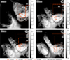 |
Fig. 10 South-centered QuACK-maps of the average surface illumination received during the 2 h prior to the respective observational periods. The figure elements and intensity scale are analogous to those in Fig. 9. |
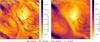 |
Fig. 11 South-centered QuACK-maps of the approximate surface acceleration, as, on 67P’s nucleus. Component parallel to the facet normal on the left, radial component on the right. The mean values within the suspected source regions are also indicated. |
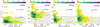 |
Fig. 12 2D histograms of the projected radial particle velocities, υrad, as a function of particle radius (for the selected particles, see Fig. 4). Because the polynomial fits to the particle tracks also approximate the particle accelerations, instead of using values averaged over a track, the particle velocities and radii were determined for each detection of a track individually and the results were weighted by the number of detections of the respective track (residence time weighting). The histogram data thus represent the weighted number of detections, Ñdet. Also shown are the approximate escape speeds at the suspected source regions, υesc (dotted line), and the corresponding maximum fall-back fractions, ϕfb (gray area). |
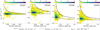 |
Fig. 13 2D histograms of the projected radial particle accelerations, arad, as a function of particle radius (for the selected particles, see Fig. 4). The histogram values were determined analogously to the description in Fig. 12. Also shown are the predicted surface acceleration, as (dotted line, see also Fig. 11), and two models (dashed and solid curves) of the particle acceleration, as described by Eqs. (8) and (9). The parameters for both curves are based on our gas models (see Sect. 4.5), but for the solid curve, a local gas production rate was assumed that is about five times higher. |
4.5 Dust coma simulations
To put our observations into perspective, we used an enhanced version of the water and dust coma modeling software by Marschall et al. (2020b) to simulate the particle dynamics around 67P and its diffuse coma during the time of our observations. The enhanced version of this software now also takes solar radiation pressure, centrifugal force, Coriolis force, and solar tides into account, and allows us to give particles an initial velocity normal to the shape model’s surface facet from which they are released. The initial velocities are drawn from a Maxwell-Boltzmann distribution defined via its peak value, υinit (which is the value we refer to as initial velocity in the following), and are assigned to all particles indiscriminately, even if the modeled gas pressure is theoretically not strong enough to lift them.
For each of the four sequences, we chose the static gas solution that best matched their respective observational conditions (see Fig. D.1). The solutions were all computed for epoch 16 of Marschall et al. (2020b), which covers the time period from Dec. 7, 2015 to Jan. 12, 2016, when 67P was roughly 1.98 AU from the Sun at a sub-solar latitude of −18.2° (which is right at the center of the sequences’ latitude value range, see Table 2). The solution setups only differ in sub-solar longitude, where we used 150° for sequence STP087, 210° for sequences STP088 and STP089, and 240° for sequence STP090. All three values almost exactly coincide with the centers of the covered sub-solar latitude value ranges of the respective sequences (see Table 2).
Based on these three gas solutions, we then simulated nine different scenarios for each of our sequences. The scenarios are defined by every combination of three different initial velocities (0, 0.25, and 0.5 m s−1) and three different activity distributions: only local (i.e., Khonsu, Atum, and Anubis), global, and nonlocal (i.e., global without local activity). For each of these runs, we simulated spherical particles in 17 different size bins distributed logarithmically over a radius range from 10−8 to 1 m, where each particle has the same bulk density as the nucleus (533 kg m−3, Pätzold et al. 2016). To reduce computation time however, we only allowed for one particle to be emitted per model facet and size regime6.
Figures D.2–D.5 show the results from the particle trajectory simulations for particle sizes similar to those we obtained from the OSIRIS data. For each sequence, initial velocity, and size bin, we randomly selected (up to) 150 simulated particles that were ejected from within the suspected source regions, and projected their trajectories onto the 2D planes of the corresponding OSIRIS/NAC FOVs (via SpiceyPy, a Python wrapper for SPICE, Annex et al. 2020). The trajectories start with the beginning of each sequence (the nucleus shapes in their initial configurations are shown for reference), and unless they leave the FOV, they represent the particle motions over a time period of up to 2 h. The simulated particles however do not (and are not intended to) retrace our observations. We merely use these simulated particle ensembles to compare them to our observations regarding their general appearance and statistical properties.
According to Figs. D.2–D.5, the initial velocities are essential for reproducing our observed particle tracks (cf. Fig. 4). Of the tested values, υinit = 0.5 m s−1 provides the best results for all sequences, which is remarkably similar to the average value we derived from the OSIRIS data (0.59 m s−1). In the case of our model, the initial velocities are also not only necessary for ejecting decimeter-sized particles at all, but also for recreating the observed ejection cones. This indicates that besides the particle speed, the shape of the ejection cones may most notably be affected by the local topography. Without the initial velocity, the simulated trajectories of the larger particles appear to "bend" predominantly in either the clockwise or counterclockwise direction, an effect caused by the viewing geometry and the rotation of the nucleus. Yet when particles are ejected with enough speed from surface areas that face in the opposite direction, their trajectories also appear to bend the other way. In the case of sequence STP090 however, even an initial velocity of 0.5 m s−1 is not enough to reproduce the almost symmetric shape of the observed ejection cone (cf. Figs. 4 and D.5).
Despite the initial velocities however, the overall projected (radial) accelerations and velocities of the simulated particles are still lower than what we measured for the real particles (cf. Figs. 12, 13, and D.6). This indicates that even higher initial velocities, locally higher gas production rates (especially of CO2, which was not included in the simulations), or lower particle bulk densities (as discussed in Sec. 4.4), may be necessary to reproduce our observations. We also did not model rocket forces, which might have a noticeable effect.
We additionally used the same simulated data from which we recovered the individual trajectories to generate images of the diffuse dust coma as it appeared in the first image of each sequence (cf. Figs. 2 and A.1). In this case, particles from every simulated size bin in the range from 10−8 to 1 m contributed. Generally, we find that the simulated images fit our observations well (but because we ran 36 different simulations, we do not present all the results here). As an example, Figs. D.7–D.10 show the dust coma simulations of sequence STP090 for all three activity distributions (local, nonlocal, and global), given υinit = 0.5 m s−1. The first three of these figures primarily illustrate how the coma simulations are affected by different particle SFDs, which are modeled according to a power law (see, e.g., Eq. (3) and the discussion in Sec. 4.2). By visually comparing the diffuse coma structures in these images to those recorded in the OSIRIS images, we find that power-law indices between 3 and 3.5 best reproduce our observations, across all sequences. This agrees well with the value range that we derived for our real, decimeter-sized particles (3.4 ± 0.3–3.8 ± 0.4, see Sec. 4.2), suggesting that a single power-law exponent can describe the SFD of both small and large particles.
By comparing the results from the three different activity distributions across all sequences, we also find further evidence that the locations of our suspected source regions are likely correct. For one, images with only local activity show strong dust features above the suspected source regions similar to our observations. Secondly, images with nonlocal activity show that the space above the suspected source regions is only significantly "contaminated" by dust features from other areas in the cases where the particle SFDs are steep. Because the corresponding particles are much smaller and faster than the particles that we observed however, their contamination is irrelevant. In the relevant particle size range, only relatively weak dust features from other areas appear above the suspected source regions (see Fig. D.10). Still, in the case of sequence STP090, such contamination might at least in part explain the missing left side of the simulated ejection cone (cf. Figs. 4 and D.5), by creating an optical illusion akin to the jet-like features described by Shi et al. (2018). Another reason might be that our gas solutions are static and do not follow the rotation of the nucleus. Depending on the viewing geometry and on how strongly the particles couple with the gas, this could also noticeably affect the projected trajectories.
Like the trajectory simulations, the coma simulations also match our observations best when the initial velocity is highest, as demonstrated by Figs. D.11–D.14 (for the case of sequence STP087). Clearly, the initial velocity strongly affects the features generated by the largest particles, which seem to make up an essential part of the simulated diffuse coma. The figures also show that different surface regions require different particle SFDs to best reproduce the observed dust features. In the case of sequence STP087 for example, the features near the suspected source region that radiate toward the top right corner are well described by a power-law index b ≈ 3, while the features on the opposite side that radiate toward the top left corner are better described by a power-law index of at least 3.5.
Finally, Fig. D.14 shows that our model failed to reproduce the strong diffuse coma features seen in the lower right corner of the first image of sequence STP087 (cf. Fig. 2). These features may have resulted from night-time activity driven by water ice sublimation and sustained by thermal lag, akin to the sunset jets discussed by Shi et al. (2016), or possibly even from CO2 ice sublimation (Gerig et al. 2018, 2020; Pinzón-Rodríguez et al. 2021).
5 Summary and conclusions
We analyzed the dynamics and potential origins of 409 decimeter-sized dust particles that were recorded in four OSIRIS/NAC image sequences of 67P’s near-nucleus dust coma between December 16, 2015, and January 6, 2016 (post-perihelion). After tracking thousands of individual dust particles though these sequences, we identified four concentrated groups of recently ejected particles and traced them back to four suspected source regions on the nucleus surface. This allowed us not only to examine their potential origins, but also to derive their approximate sizes, speeds, and accelerations. Finally, we compared our observations and results to simulations of 67P’s dust coma for further evaluation.
Although we were limited to tracking particles only in the 2D image plane and not in the full 3D environment, our data analysis provides much evidence that the general locations of the suspected source regions are likely correct:
- (i)
The particle trajectories form distinct ejection cones that taper toward the centers of the suspected source regions.
- (ii)
Even though the suspected source regions were chosen independently from one another, they turned out to be rather well confined and to strongly overlap.
- (iii)
The suspected source regions contain (or are near) areas where global activity models estimate high surface erosion and gas emission rates (Combi et al. 2020; Läuter et al. 2022).
- (iv)
In particular, the suspected source regions derived from image sequences STP087 and STP089 largely coincide with an area in the Khonsu region for which a lot of activity and surface changes have been documented (e.g., Deshapriya et al. 2016; Hasselmann et al. 2019).
- (v)
Unlike other areas, the suspected source regions were continuously well illuminated during the observational periods and the roughly 4 h in local time leading up to them.
- (vi)
Trajectory simulations of particles released from the suspected source regions generally reproduce the observed particle tracks well.
- (vii)
Comparisons between different simulations of the diffuse dust coma (local vs. nonlocal) show that most of the simulated dust features above the suspected source regions come from local activity.
Throughout this paper, we drew several conclusions regarding the nature of the observed activity:
- (i)
Instead of homogeneous activity, the ejection of large particles (⪆1 cm) can occur distinctly localized.
- (ii)
The concentrated ejection of large particles does not necessarily correlate (in strength, location, or orientation) with that of small particles (⪅1 cm) that make up the diffuse coma. This may be evidence that water-driven erosion and CO2-driven ejection of large chunks cannot happen simultaneously at the same location.
- (iii)
The suspected source regions of the particles that we traced back to the nucleus surface predominantly lie in the Khonsu-Atum-Anubis area, and the observed activity may be linked to rugged terrain or steep slopes like scarps, cliffs, or fractures.
- (iv)
The studied particles range in size from about 5 cm to 1.15 m in (equivalent) radius. Power-law fits to their SFDs best describe the data with power-law indices between 3.4 ± 0.3 and 3.8 ± 0.4. This indicates that shortly after ejection, most of the mass is still contained in the larger particles, although ultimately most of them likely did not escape the nucleus gravity. The index values also agree notably well with those obtained for submillimeter-sized particles (3.7 and 3.1 ± 0.5, Fulle et al. 2016; Merouane et al. 2016), and might reflect an SFD transition of the surface material located in the suspected source regions (Deshapriya et al. 2016; Hasselmann et al. 2019).
- (v)
Solar irradiation alone cannot explain the locality of the observed activity. Additionally, surface accelerations in the suspected source regions are relatively high, ruling out gravity and centrifugal forces as decisive factors as well.
- (vi)
The projected radial particle velocities directly provide upper limit estimates for the particle fall-back fractions, which lie between 75 and 91%. The data indicate that essentially all particles larger than 40 cm likely fell back onto the nucleus surface.
- (vii)
The distributions of the projected radial particle accelerations as functions of the particle radii are well described by the local surface acceleration (lower bound) and gas drag (upper bound). The gas drag parameters, however, are degenerate and cannot be precisely constrained. Values from our water and dust coma simulations nevertheless indicate that the local gas production rate was likely several times higher (Qg = 3.6 × 10⁻⁵ kg s−1 m−2) than the prediction by our purely insolation-driven model and the peak average production rates estimated by Läuter et al. (2022).
- (viii)
Some particles exhibit downward accelerations that are much stronger than the local surface accelerations. Most of these outliers are likely caused by inaccurate measurements and statistical effects, but their general trend might also be a sign of asymmetric outgassing.
- (ix)
Rough estimates of the initial particle velocities are distinctly nonzero and average around 0.59 m s−1, which indicates that the particles likely gained most of their speed from the initial ejection event.
- (x)
Our dynamics simulations of decimeter-sized particles in the coma of 67P support the need for higher local activity to reproduce the observed trajectories. Simulated particles larger than ≈32 cm could not be lifted from the suspected source regions without introducing initial velocities in addition to gas drag. Even with an initial velocity of ≈0.5 m s−1 the simulated particles were generally still slower than those we observed.
- (xi)
The inclusion of initial velocities also shows that they are necessary for reproducing the observed ejection cones, which indicates that the local topography plays an important role in shaping these cones.
- (xii)
Both, the simulated dynamics of individual particles, and the simulated images of the diffuse dust coma, match the observations best when the initial velocity is the highest (≈0.5 m s−1). This is further evidence that initial velocities are an essential aspect of the ejection process.
- (xiii)
The simulated images additionally reproduce our observations best given particle SFDs described by power laws with indices equal to 3 or 3.5. This agrees well with the value range that we obtained from our real particle populations, but we also found that some dust features require different size distributions to be well reproduced.
Overall, our observational and modeling results strongly suggest that the concentrated local ejection of decimeter-sized particles cannot be explained with water-driven activity and favorable illumination conditions alone. Instead, the composition and structure of the suspected source regions seem to be the deciding factors; of these, we deem an overabundance of volatiles, in particular of CO2 ice, to be the most probable cause. This is in line with current particle ejection models (e.g., Gundlach et al. 2020; Fulle et al. 2020; Wesołowski et al. 2020; Ciarniello et al. 2022; Davidsson et al. 2022), which necessitate the sublimation of CO2 ice in deeper surface layers to eject decimeter-sized particles. Additionally, our results show that decimeter-sized particles are very likely ejected with substantial nonzero initial velocities, which agrees well with other recent studies (e.g., Bischoff et al. 2019; Lemos et al. 2023, 2024; Kwon et al. 2023; Shi et al. 2024), and implies that the ejection mechanism must be considerably more energetic than a slow or gradual liftoff.
Acknowledgements
We thank the anonymous referee for their valuable feedback; Xian Shi, Nicholas Attree, Yuri Skorov, Marco Fulle, and Asmus Freitag for (proof)reading our manuscript and providing helpful comments; Miryam Merk, for statistical consulting; Sonia Fornasier, Matthias Läuter, and Tobias Kramer for providing their data; Aaron Clauset for discussing the intricacies of power-law fitting with us; and Pedro Hasselmann, Maurizio Pajola, Mohamed Ramy El-Maarry, Nicolas Thomas, Frank Preusker, Michael Combi, Koji Wada, Jean-Baptiste Vincent, Johannes Markkanen, and Giovanna Rinaldi for providing tools and discussing certain aspects of our paper. We acknowledge the operation and calibration team at MPS and the Principal Investigator Holger Sierks on behalf of the OSIRIS Team for providing the OSIRIS images and related data sets. OSIRIS was built by a consortium of the Max-Planck-Institut für Sonnensystemforschung, Göttingen, Germany; the CISAS University of Padova, Italy; the Laboratoire d’Astrophysique de Marseille, France; the Instituto de Astrofísica de Andalucia, CSIC, Granada, Spain; the Research and Scientific Support Department of the European Space Agency, Noordwijk, The Netherlands; the Instituto Nacional de Técnica Aeroespacial, Madrid, Spain; the Universidad Politéchnica de Madrid, Spain; the Department of Physics and Astronomy of Uppsala University, Sweden; and the Institut für Datentechnik und Kommunikationsnetze der Technischen Universität Braunschweig, Germany. The support of the national funding agencies of Germany (DLR), France (CNES), Italy (ASI), Spain (MEC), Sweden (SNSB), and the ESA Technical Directorate is gratefully acknowledged. We thank the Rosetta Science Ground Segment at ESAC, the Rosetta Missions Operations Centre at ESOC and the Rosetta Project at ESTEC for their outstanding work enabling the science return of the Rosetta Mission. M.P., J.A., and P.L. acknowledge funding by the ERC Starting Grant No. 757390 Comet and Asteroid Re-Shaping through Activity (CAstRA). J.A. acknowledges funding by the Volkswagen Foundation. M.P. and P.L. conducted the work in this paper in the framework of the International Max-Planck Research School (IMPRS) for Solar System Science at the University of Göttingen.
Appendix A Sample images from sequences STP089 and STP090
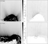 |
Fig. A.1 Sample images from sequences STP089 and STP090. The first images of the respective sequences are on the left, the master images on the right. The ellipses in the master images mark the suspected source regions of the concentrated particle groups. All images are brightness-inverted and had their contrasts improved for better readability (continuation of Fig. 2). |
Appendix B Reasons for rejection of image sequences
In the following, we list the reasons why we excluded other OSIRIS image sequences from our analysis (roughly from most to least critical): – An incomplete pair of subsequences (i.e., only one exists) or an insufficient number of images (many subsequences consist of less than twenty images). If the covered time period is long, subsequent particle detections can lie far apart, which makes particle tracking very difficult, especially if there is no "stem" of detections linked over a short interval (cf. Fig. 1), that provides accurate predictions. Conversely, if the covered time period is short, the derived particle dynamics can be unreliable because the tracks do not evolve enough for fits to be resistant against smaller deviations like pointing fluctuations or the inclusion of unrelated detections.
Binning, which severely hampers particle detection.
A lack of sidereal objects, which are needed to correct for pointing fluctuations.
An abrupt and substantial change in (commanded) camera pointing, which is nontrivial to correct for, and makes visual confirmation of particle tracks mostly impossible.
Long time gaps/periods, which make the continuous tracking of the same particles difficult and result in many particles to have left the FOV.
No concentrated group(s) of particles that seemingly originate from the same surface area (see Sec. 3.2 as to why this is important).
A low number of (reliable) tracks (e.g., due to a low number of particles).
Nucleus outside the FOV, which makes associating particles with potential source regions on its surface much more speculative.
Too large nucleocentric distances of the spacecraft, which do not allow for particles near the nucleus to be distinguishable from the diffuse coma or associated with potential source regions.
Different time signatures (i.e., images come in singles or triplets instead of pairs, which require at minimum an adaptation of the tracking algorithm).
Missing or an uneven number of images (e.g., in the used calibration levels).
Defect/artifact-riddled/incomplete images (see, e.g., the artifacts around the nucleus in the first image of sequence STP088, shown in Fig. 2).
Appendix C Caveats of polynomial fitting
As Figure 3 shows, fitting third-order polynomials is sometimes not only required for tracking particles successfully, but often simply the more appropriate choice. From a physical standpoint, third-order polynomials are justified, since the particle acceleration changes over time due to the complex gas and micro-gravity environment and the possibility for asymmetric outgassing. Even fourth-order polynomials may be fair. Yet because of residual pointing fluctuation and other effects, the positional data of our particles are not precise enough to allow for the detection of such delicate signals. In some cases, the order of the fitted polynomial can also substantially affect the derived velocity and acceleration vectors and change the extrapolated course of the track (see Fig. C.1 for an extreme example). Our ability to extrapolate particle tracks is thus limited, which is one reason why we only trace back particles for at most half an hour.
To ensure that our statistical results are nonetheless reliable, we tested how much they are affected by the order of the fitted polynomials (second or third). The most notable difference was in the track populations that intersect with the suspected source regions. Some tracks only do so when using a second- but not a third-order polynomial, and others vice versa. The corresponding radius, velocity, and acceleration distributions, however, are very similar, and do not significantly change the derived qualities. The fitted SFD power-law indices, for example, differ by no more than 0.1. Based on this analysis, we consider our statistical results reliable, and our conclusions remain unaffected.
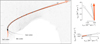 |
Fig. C.1 Same particle track shown in Fig. 3 (white circles), but this time fitted with a second-, third-, and fourth-order polynomial, each extrapolated an hour back and over two and a half hours forward in time. The plots on the right show the respective derived vertical and horizontal particle velocities and accelerations at t = 0 s. |
Appendix D Dust coma simulation results
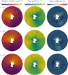 |
Fig. D.1 Properties of the three static gas solutions that we used for our dust coma models. The plots show model cross sections that slice through the suspected source regions, which are indicated by the bold dashed curves on the top left side of the nucleus. The solar directions are highlighted by the white lines. The drag coefficient plots show the results computed for global activity of 32 cm particles, which are representative for the whole relevant size range from 1 cm to 1 m. The circular artifacts in these plots, around 3 km from the nucleus, are a consequence of how the simulation domain was built (with a transition region between an inner sphere with very small cells and an outer region with much larger cells) and the low number of simulated particles. |
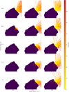 |
Fig. D.2 Trajectory simulations of up to 150 randomly selected particles ejected from within the suspected source region of sequence STP087. |
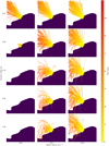 |
Fig. D.3 Trajectory simulations of up to 150 randomly selected particles ejected from within the suspected source region of sequence STP088. |
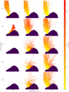 |
Fig. D.4 Trajectory simulations of up to 150 randomly selected particles ejected from within the suspected source region of sequence STP089. |
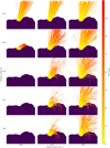 |
Fig. D.5 Trajectory simulations of up to 150 randomly selected particles ejected from within the suspected source region of sequence STP090. |
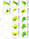 |
Fig. D.6 Projected radial accelerations and velocities of the particles shown in Fig. D.5 (sequence STP090). As with the OSIRIS data, the values were determined by fitting third-order polynomials to the projected tracks. In each subplot, the x-axis shows the projected radial velocity in m s−1, the y-axis the projected radial acceleration in m s−2, and the color bar the number of measurements, which are again weighted by the number of measurements per respective track (residence time weighting). The three bottom left panels are blank because no particles were ejected in these instances. |
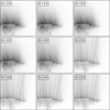 |
Fig. D.7 Coma simulations for sequence STP090 as a function of the particle SFD power-law index, b, given local activity and υirit = 0.5 m s 1. |
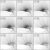 |
Fig. D.8 Coma simulations for sequence STP090 as a function of the particle SFD power-law index, b, given nonlocal activity and υinit = 0.5 m s−1. |
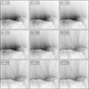 |
Fig. D.9 Coma simulations for sequence STP090 as a function of the particle SFD power-law index, b, given global activity and υinit = 0.5 m s−1. |
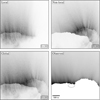 |
Fig. D.10 Comparison between coma simulations with different activity distributions given υinit = 0.5 m s−1, and the observed coma in the first image of sequence STP090. The image of the observed coma is the background signal that we subtracted during the preparation for the tracking procedure (see Sect. 2 and Pfeifer et al. 2022). The ellipse indicates the suspected source region. All images are brightness-inverted and had their contrasts improved individually for better reading. Because of this, the absolute intensity levels should not be compared across images, but only relative to other areas of the same image. |
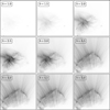 |
Fig. D.11 Global coma simulations for sequence STP087 as a function of the particle SFD power-law index, b, given υinit = 0.0 m s−1. |
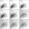 |
Fig. D.12 Global coma simulations for sequence STP087 as a function of the particle SFD power-law index, b, given υinit = 0.25 m s−1. |
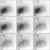 |
Fig. D.13 Global coma simulations for sequence STP087 as a function of the particle SFD power-law index, b, given υinit = 0.5 m s−1. |
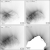 |
Fig. D.14 Comparison between global coma simulations given different initial velocities, υinit, and the observed coma in the first image of sequence STP087. The image of the observed coma is the background signal subtracted during the preparation for the tracking procedure (see Sect. 2 and Pfeifer et al. 2022). The ellipse indicates the suspected source region. All images are brightness-inverted and had their contrasts improved individually for better readability. Because of this, the absolute intensity levels should not be compared across images, but only relative to other areas of the same image. |
References
- Acton, C. H. 1996, Planet. Space Sci., 44, 65 [Google Scholar]
- Agarwal, J., Müller, M., Reach, W. T., et al. 2010, Icarus, 207, 992 [NASA ADS] [CrossRef] [Google Scholar]
- Agarwal, J., A’Hearn, M. F., Vincent, J.-B., et al. 2016, MNRAS, 462, S78 [Google Scholar]
- Agarwal, J., Della Corte, V., Feldman, P. D., et al. 2017, MNRAS, 469, s606 [NASA ADS] [CrossRef] [Google Scholar]
- Agarwal, J., Kim, Y., Kelley, M. S. P., & Marschall, R. 2023, arXiv e-prints [arXiv:2309.12759] [Google Scholar]
- Alstott, J., Bullmore, E., & Plenz, D. 2014, PLOS ONE, 9, e85777 [NASA ADS] [CrossRef] [Google Scholar]
- Annex, A. M., Pearson, B., Seignovert, B., et al. 2020, J. Open Source Softw., 5, 2050 [CrossRef] [Google Scholar]
- Arakawa, M., Wada, K., Saiki, T., et al. 2017, Space Sci. Rev., 208, 187 [NASA ADS] [CrossRef] [Google Scholar]
- Arakawa, M., Saiki, T., Wada, K., et al. 2020, Science, 368, 67 [NASA ADS] [CrossRef] [Google Scholar]
- Attree, N., Groussin, O., Jorda, L., et al. 2018a, A&A, 611, A33 [NASA ADS] [CrossRef] [EDP Sciences] [Google Scholar]
- Attree, N., Groussin, O., Jorda, L., et al. 2018b, A&A, 610, A76 [NASA ADS] [CrossRef] [EDP Sciences] [Google Scholar]
- Auger, A.-T., Groussin, O., Jorda, L., et al. 2015, A&A, 583, A35 [NASA ADS] [CrossRef] [EDP Sciences] [Google Scholar]
- A’Hearn, M. F., Belton, M. J. S., Delamere, W. A., et al. 2011, Science, 332, 1396 [CrossRef] [Google Scholar]
- Barbary, K. 2016, J. Open Source Softw., 1, 58 [Google Scholar]
- Belton, M. J. S. 2010, Icarus, 210, 881 [NASA ADS] [CrossRef] [Google Scholar]
- Bertin, E., & Arnouts, S. 1996, A&ASS, 117, 393 [NASA ADS] [CrossRef] [EDP Sciences] [Google Scholar]
- Bird, G. A. 1994, Molecular Gas Dynamics And The Direct Simulation Of Gas Flows (Oxford: Clarendon Press) [Google Scholar]
- Bischoff, D., Gundlach, B., Neuhaus, M., & Blum, J. 2019, MNRAS, 483, 1202 [Google Scholar]
- Bischoff, D., Schuckart, C., Attree, N., Gundlach, B., & Blum, J. 2023, MNRAS, 523, 5171 [NASA ADS] [CrossRef] [Google Scholar]
- Blum, J., Gundlach, B., Krause, M., et al. 2017, MNRAS, 469, S755 [Google Scholar]
- Blum, J., Bischoff, D., & Gundlach, B. 2022, Universe, 8, 381 [CrossRef] [Google Scholar]
- Brown, W. K. 1989, J. Astrophys. Astron., 10, 89 [NASA ADS] [CrossRef] [Google Scholar]
- Cambianica, P., Cremonese, G., Naletto, G., et al. 2019, A&A, 630, A15 [NASA ADS] [CrossRef] [EDP Sciences] [Google Scholar]
- Cambianica, P., Fulle, M., Cremonese, G., et al. 2020, A&A, 636, A91 [EDP Sciences] [Google Scholar]
- Chesley, S. R., French, A. S., Davis, A. B., et al. 2020, J. Geophys. Res.: Planets, 125 [Google Scholar]
- Choukroun, M., Altwegg, K., Kührt, E., et al. 2020, Space Sci. Rev., 216, 44 [CrossRef] [Google Scholar]
- Ciarniello, M., Fulle, M., Raponi, A., et al. 2022, Nat. Astron., 6, 546 [NASA ADS] [CrossRef] [Google Scholar]
- Cigala, V., Kueppers, U., Peña Fernández, J. J., et al. 2017, J. Geophys. Res.: Solid Earth, 122, 6031 [NASA ADS] [CrossRef] [Google Scholar]
- Cigala, V., Kueppers, U., Fernández, J. J. P., & Dingwell, D. B. 2021, Bull. Volcanol., 83, 53 [NASA ADS] [CrossRef] [Google Scholar]
- Clark, B. C., Green, S. F., Economou, T. E., et al. 2004, J. Geophys. Res.: Planets, 109, E12S03 [Google Scholar]
- Clauset, A., Shalizi, C. R., & Newman, M. E. J. 2009, SIAM Rev., 51, 661 [NASA ADS] [CrossRef] [Google Scholar]
- Combi, M., Shou, Y., Fougere, N., et al. 2020, Icarus, 335, 113421 [NASA ADS] [CrossRef] [Google Scholar]
- Crifo, J. F., Itkin, A. L., & Rodionov, A. V. 1995, Icarus, 116, 77 [NASA ADS] [CrossRef] [Google Scholar]
- Crifo, J. F., Loukianov, G. A., Rodionov, A. V., & Zakharov, V. V. 2005, Icarus, 176, 192 [NASA ADS] [CrossRef] [Google Scholar]
- Davidsson, B. J. R., Sierks, H., Güttler, C., et al. 2016, A&A, 592, A63 [NASA ADS] [CrossRef] [EDP Sciences] [Google Scholar]
- Davidsson, B. J. R., Birch, S., Blake, G. A., et al. 2021, Icarus, 354, 114004 [NASA ADS] [CrossRef] [Google Scholar]
- Davidsson, B. J. R., Schloerb, F. P., Fornasier, S., et al. 2022, MNRAS, 516, 6009 [NASA ADS] [CrossRef] [Google Scholar]
- Deshapriya, J. D. P., Barucci, M. A., Fornasier, S., et al. 2016, MNRAS, 462, S274 [NASA ADS] [CrossRef] [Google Scholar]
- Deshapriya, J. D. P., Barucci, M. A., Fornasier, S., et al. 2018, A&A, 613, A36 [NASA ADS] [CrossRef] [EDP Sciences] [Google Scholar]
- Dohnanyi, J. S. 1969, J. Geophys. Res., 74, 2531 [Google Scholar]
- El-Maarry, M. R., Thomas, N., Giacomini, L., et al. 2015, A&A, 583, A26 [NASA ADS] [CrossRef] [EDP Sciences] [Google Scholar]
- El-Maarry, M. R., Thomas, N., Gracia-Berná, A., et al. 2016, A&A, 593, A110 [NASA ADS] [CrossRef] [EDP Sciences] [Google Scholar]
- El-Maarry, M. R., Groussin, O., Thomas, N., et al. 2017a, Science, 355, 1392 [Google Scholar]
- El-Maarry, M. R., Thomas, N., Gracia-Berná, A., et al. 2017b, A&A, 598, C2 [NASA ADS] [CrossRef] [EDP Sciences] [Google Scholar]
- ESA SPICE Service 2020, Rosetta Operational SPICE Kernel Dataset, https://doi.org/10.5270/esa-tyidsbu [Google Scholar]
- Ezekiel, M. 1930, Methods Of Correlation Analysis (John Wily & Sons Inc) [Google Scholar]
- Fagents, S. A., Lopes, R. M. C., Quick, L. C., & Gregg, T. K. P. 2022, in Comparative Planetology, 1, Planetary Volcanism across the Solar System, eds. T. K. P. Gregg, R. M. C. Lopes, & S. A. Fagents (Elsevier), 161 [CrossRef] [Google Scholar]
- Fahrmeir, L., Kneib, T., Lang, S., & Marx, B. D. 2021, Regression: Models, Methods and Applications (Springer) [CrossRef] [Google Scholar]
- Feller, W. 1948, Ann. Math. Stat., 19, 177 [CrossRef] [Google Scholar]
- Ferrari, S., Penasa, L., La Forgia, F., et al. 2018, MNRAS, 479, 1555 [NASA ADS] [CrossRef] [Google Scholar]
- Finson, M. L., & Probstein, R. F. 1968, ApJ, 154, 327 [NASA ADS] [CrossRef] [Google Scholar]
- Finson, M. L., & Probstein, R. F. 1968b, ApJ, 154, 353 [NASA ADS] [CrossRef] [Google Scholar]
- Fornasier, S., Mottola, S., Keller, H. U., et al. 2016, Science, 354, 1566 [NASA ADS] [CrossRef] [Google Scholar]
- Fornasier, S., Feller, C., Lee, J.-C., et al. 2017, MNRAS, 469, S93 [NASA ADS] [CrossRef] [Google Scholar]
- Fornasier, S., Hoang, V. H., Hasselmann, P. H., et al. 2019, A&A, 630, A7 [NASA ADS] [CrossRef] [EDP Sciences] [Google Scholar]
- Fornasier, S., Hoang, H. V., Fulle, M., Quirico, E., & Ciarniello, M. 2023, A&A, 672, A136 [NASA ADS] [CrossRef] [EDP Sciences] [Google Scholar]
- Fowler, A. C., & Scheu, B. 2016, Proc. Roy. Soc. A: Math. Phys. Eng. Sci., 472, 20150843 [Google Scholar]
- Frattin, E., Bertini, I., Ivanovski, S. L., et al. 2021, MNRAS, 504, 4687 [NASA ADS] [CrossRef] [Google Scholar]
- Fulle, M. 1989, A&A, 217, 283 [NASA ADS] [Google Scholar]
- Fulle, M., Colangeli, L., Agarwal, J., et al. 2010, A&A, 522, A63 [NASA ADS] [CrossRef] [EDP Sciences] [Google Scholar]
- Fulle, M., Marzari, F., Corte, V. D., et al. 2016, ApJ, 821, 19 [NASA ADS] [CrossRef] [Google Scholar]
- Fulle, M., Blum, J., Rotundi, A., et al. 2020, MNRAS, 493, 4039 [CrossRef] [Google Scholar]
- Gerig, S.-B., Marschall, R., Thomas, N., et al. 2018, Icarus, 311, 1 [NASA ADS] [CrossRef] [Google Scholar]
- Gerig, S.-B., Pinzón-Rodríguez, O., Marschall, R., Wu, J.-S., & Thomas, N. 2020, Icarus, 351, 113968 [CrossRef] [Google Scholar]
- Giacomini, L., Massironi, M., El-Maarry, M. R., et al. 2016, MNRAS, 462, S352 [NASA ADS] [CrossRef] [Google Scholar]
- Grieger, B. 2019, A&A, 630, A1 [NASA ADS] [CrossRef] [EDP Sciences] [Google Scholar]
- Groussin, O., Jorda, L., Auger, A.-T., et al. 2015, A&A, 583, A32 [NASA ADS] [CrossRef] [EDP Sciences] [Google Scholar]
- Gundlach, B., Blum, J., Keller, H. U., & Skorov, Y. V. 2015, A&A, 583, A12 [NASA ADS] [CrossRef] [EDP Sciences] [Google Scholar]
- Gundlach, B., Fulle, M., & Blum, J. 2020, MNRAS, 493, 3690 [NASA ADS] [CrossRef] [Google Scholar]
- Güttler, C., Hasselmann, P. H., Li, Y., et al. 2017, MNRAS, 469, S312 [CrossRef] [Google Scholar]
- Güttler, C., Mannel, T., Rotundi, A., et al. 2019, A&A, 630, A24 [NASA ADS] [CrossRef] [EDP Sciences] [Google Scholar]
- Hartmann, W. K. 1969, Icarus, 10, 201 [NASA ADS] [CrossRef] [Google Scholar]
- Hasselmann, P. H., Barucci, M. A., Fornasier, S., et al. 2019, A&A, 630, A8 [NASA ADS] [CrossRef] [EDP Sciences] [Google Scholar]
- Hilchenbach, M., Kissel, J., Langevin, Y., et al. 2016, ApJ, 816, L32 [CrossRef] [Google Scholar]
- Höfner, S., Vincent, J.-B., Blum, J., et al. 2017, A&A, 608, A121 [Google Scholar]
- Huebner, W. F., Benkhoff, J., Capria, M.-T., et al. 2006, Heat And Gas Diffusion in Comet Nuclei (International Space Science Institute) [Google Scholar]
- Ishiguro, M. 2008, Icarus, 193, 96 [NASA ADS] [CrossRef] [Google Scholar]
- Ivanovski, S., Zakharov, V., Della Corte, V., et al. 2017a, Icarus, 282, 333 [NASA ADS] [CrossRef] [Google Scholar]
- Ivanovski, S. L., Della Corte, V., Rotundi, A., et al. 2017b, MNRAS, 469, S774 [NASA ADS] [CrossRef] [Google Scholar]
- Jiang, Y., & Schmidt, J. 2020, Heliyon, 6, e05275 [NASA ADS] [CrossRef] [Google Scholar]
- Jorda, L., Gaskell, R., Capanna, C., et al. 2016, Icarus, 277, 257 [Google Scholar]
- Keller, H. U., Delamere, W. A., Reitsema, H. J., Huebner, W. F., & Schmidt, H. U. 1987, A&A, 187, 807 [NASA ADS] [Google Scholar]
- Keller, H. U., Barbieri, C., Lamy, P., et al. 2007, Space Sci. Rev., 128, 433 [Google Scholar]
- Keller, H. U., Mottola, S., Davidsson, B., et al. 2015, A&A, 583, A34 [NASA ADS] [CrossRef] [EDP Sciences] [Google Scholar]
- Keller, H. U., Mottola, S., Hviid, S. F., et al. 2017, MNRAS, 469, S357 [Google Scholar]
- Kelley, M. S., Reach, W. T., & Lien, D. J. 2008, Icarus, 193, 572 [NASA ADS] [CrossRef] [Google Scholar]
- Kelley, M. S., Wooden, D. H., Tubiana, C., et al. 2009, AJ, 137, 4633 [NASA ADS] [CrossRef] [Google Scholar]
- Kelley, M. S., Lindler, D. J., Bodewits, D., et al. 2013, Icarus, 222, 634 [NASA ADS] [CrossRef] [Google Scholar]
- Kelley, M. S. P., Lindler, D. J., Bodewits, D., et al. 2015, Icarus, 262, 187 [NASA ADS] [CrossRef] [Google Scholar]
- Klaus, A., Yu, S., & Plenz, D. 2011, PLOS ONE, 6, e19779 [NASA ADS] [CrossRef] [Google Scholar]
- Knollenberg, J., Lin, Z. Y., Hviid, S. F., et al. 2016, A&A, 596, A89 [NASA ADS] [CrossRef] [EDP Sciences] [Google Scholar]
- Kramer, T., & Noack, M. 2015, ApJ, 813, L33 [Google Scholar]
- Kramer, T., & Noack, M. 2016, ApJ, 823, L11 [NASA ADS] [CrossRef] [Google Scholar]
- Kwon, Y. G., Opitom, C., & Lippi, M. 2023, A&A, 674, A206 [NASA ADS] [CrossRef] [EDP Sciences] [Google Scholar]
- La Forgia, F., Giacomini, L., Lazzarin, M., et al. 2015, A&A, 583, A41 [NASA ADS] [CrossRef] [EDP Sciences] [Google Scholar]
- Lai, I.-L., Ip, W.-H., Su, C.-C., et al. 2016, MNRAS, 462, S533 [NASA ADS] [CrossRef] [Google Scholar]
- Lai, I.-L., Ip, W.-H., Lee, J.-C., et al. 2019, A&A, 630, A17 [NASA ADS] [CrossRef] [EDP Sciences] [Google Scholar]
- Läuter, M., Kramer, T., Rubin, M., & Altwegg, K. 2019, MNRAS, 483, 852 [Google Scholar]
- Läuter, M., Kramer, T., Rubin, M., & Altwegg, K. 2020, MNRAS, 498, 3995 [Google Scholar]
- Läuter, M., Kramer, T., Rubin, M., & Altwegg, K. 2022, ACS Earth Space Chem., 6, 1189 [CrossRef] [Google Scholar]
- Lee, J.-C., Massironi, M., Ip, W.-H., et al. 2016, MNRAS, 462, S573 [NASA ADS] [CrossRef] [Google Scholar]
- Lemos, P., Agarwal, J., & Schröter, M. 2023, MNRAS, 519, 5775 [CrossRef] [Google Scholar]
- Lemos, P., Agarwal, J., Marschall, R., & Pfeifer, M. 2024, A&A, submitted [NASA ADS] [CrossRef] [EDP Sciences] [Google Scholar]
- Leon-Dasi, M., Besse, S., Grieger, B., & Küppers, M. 2021, A&A, 652, A52 [NASA ADS] [CrossRef] [EDP Sciences] [Google Scholar]
- Lin, Z.-Y., Knollenberg, J., Vincent, J.-B., et al. 2017, MNRAS, 469, S731 [NASA ADS] [CrossRef] [Google Scholar]
- Liu, X., Sachse, M., Spahn, F., & Schmidt, J. 2016, J. Geophys. Res.: Planets, 121, 1141 [NASA ADS] [CrossRef] [Google Scholar]
- Lucchetti, A., Cremonese, G., Jorda, L., et al. 2016, A&A, 585, L1 [NASA ADS] [CrossRef] [EDP Sciences] [Google Scholar]
- Lucchetti, A., Pajola, M., Fornasier, S., et al. 2017, MNRAS, 469, S238 [NASA ADS] [CrossRef] [Google Scholar]
- Mandelbrot, B. B. 1982, The Fractal Geometry of Nature (San Francisco: W.H. Freeman) [Google Scholar]
- Markkanen, J., & Agarwal, J. 2020, A&A, 643, A16 [NASA ADS] [CrossRef] [EDP Sciences] [Google Scholar]
- Markkanen, J., Agarwal, J., Väisänen, T., Penttilä, A., & Muinonen, K. 2018, ApJ, 868, L16 [NASA ADS] [CrossRef] [Google Scholar]
- Marschall, R., Su, C. C., Liao, Y., et al. 2016, A&A, 589, A90 [NASA ADS] [CrossRef] [EDP Sciences] [Google Scholar]
- Marschall, R., Mottola, S., Su, C. C., et al. 2017, A&A, 605, A112 [NASA ADS] [CrossRef] [EDP Sciences] [Google Scholar]
- Marschall, R., Rezac, L., Kappel, D., et al. 2019, Icarus, 328, 104 [Google Scholar]
- Marschall, R., Liao, Y., Thomas, N., & Wu, J.-S. 2020a, Icarus, 346, 113742 [CrossRef] [Google Scholar]
- Marschall, R., Markkanen, J., Gerig, S.-B., et al. 2020b, Front. Phys., 8, 227 [NASA ADS] [CrossRef] [Google Scholar]
- Marschall, R., Skorov, Y., Zakharov, V., et al. 2020c, Space Sci. Rev., 216, 130 [Google Scholar]
- Marschall, R., Davidsson, B. J. R., Rubin, M., & Tenishev, V. 2023, arXiv e-prints [arXiv:2308.05797] [Google Scholar]
- Merouane, S., Zaprudin, B., Stenzel, O., et al. 2016, A&A, 596, A87 [NASA ADS] [CrossRef] [EDP Sciences] [Google Scholar]
- Merouane, S., Stenzel, O., Hilchenbach, M., et al. 2017, MNRAS, 469, S459 [NASA ADS] [CrossRef] [Google Scholar]
- Moreno, F., Guirado, D., Muñoz, O., et al. 2022, MNRAS, 510, 5142 [NASA ADS] [CrossRef] [Google Scholar]
- Mottola, S., Arnold, G., Grothues, H.-G., et al. 2015, Science, 349, aab0232 [Google Scholar]
- Muniruzzaman, A. N. M. 1957, Calcutta Stat. Assoc. Bull., 7, 115 [CrossRef] [Google Scholar]
- Oklay, N., Sunshine, J. M., Pajola, M., et al. 2016, MNRAS, 462, S394 [NASA ADS] [CrossRef] [Google Scholar]
- Oklay, N., Mottola, S., Vincent, J.-B., et al. 2017, MNRAS, 469, S582 [NASA ADS] [CrossRef] [Google Scholar]
- Opik, E. J. 1936, Publications of the Tartu Astrofizica Observatory, 28, 1 [NASA ADS] [Google Scholar]
- Ott, T., Drolshagen, E., Koschny, D., et al. 2017, MNRAS, 469, S276 [Google Scholar]
- Pajola, M., Vincent, J.-B., Güttler, C., et al. 2015, A&A, 583, A37 [NASA ADS] [CrossRef] [EDP Sciences] [Google Scholar]
- Pajola, M., Lucchetti, A., Vincent, J.-B., et al. 2016a, A&A, 592, A2 [NASA ADS] [CrossRef] [EDP Sciences] [Google Scholar]
- Pajola, M., Mottola, S., Hamm, M., et al. 2016b, MNRAS, 462, S242 [NASA ADS] [CrossRef] [Google Scholar]
- Pajola, M., Oklay, N., Forgia, F. L., et al. 2016c, A&A, 592, A69 [NASA ADS] [CrossRef] [EDP Sciences] [Google Scholar]
- Pajola, M., Höfner, S., Vincent, J. B., et al. 2017a, Nat. Astron., 1, 0092 [NASA ADS] [CrossRef] [Google Scholar]
- Pajola, M., Lucchetti, A., Fulle, M., et al. 2017b, MNRAS, 469, S636 [Google Scholar]
- Pajola, M., Lee, J.-C., Oklay, N., et al. 2019, MNRAS, 485, 2139 [NASA ADS] [CrossRef] [Google Scholar]
- Pätzold, M., Andert, T., Hahn, M., et al. 2016, Nature, 530, 63 [CrossRef] [Google Scholar]
- Pfeifer, M., Agarwal, J., & Schröter, M. 2022, A&A, 659, A171 [NASA ADS] [CrossRef] [EDP Sciences] [Google Scholar]
- Pinzón-Rodríguez, O., Marschall, R., Gerig, S.-B., et al. 2021, A&A, 655, A20 [NASA ADS] [CrossRef] [EDP Sciences] [Google Scholar]
- Pommerol, A., Thomas, N., El-Maarry, M. R., et al. 2015, A&A, 583, A25 [NASA ADS] [CrossRef] [EDP Sciences] [Google Scholar]
- Poulet, F., Lucchetti, A., Bibring, J.-P., et al. 2016, MNRAS, 462, S23 [Google Scholar]
- Quick, L. C., Barnouin, O. S., Prockter, L. M., & Patterson, G. W. 2013, Planet. Space Sci., 86, 1 [NASA ADS] [CrossRef] [Google Scholar]
- Reshetnyk, V. M., Skorov, Y. V., Lacerda, P., Hartogh, P., & Rezac, L. 2018, Solar Syst. Res., 52, 266 [NASA ADS] [CrossRef] [Google Scholar]
- Reshetnyk, V., Skorov, Y., Vasyuta, M., et al. 2021, Solar Syst. Res., 55, 106 [NASA ADS] [CrossRef] [Google Scholar]
- Reshetnyk, V., Skorov, Y., Bentley, M., et al. 2022, Solar Syst. Res., 56, 100 [NASA ADS] [CrossRef] [Google Scholar]
- Rinaldi, G., Della Corte, V., Fulle, M., et al. 2017, MNRAS, 469, S598 [NASA ADS] [CrossRef] [Google Scholar]
- Rodionov, A. V., Crifo, J. F., Szegő, K., Lagerros, J., & Fulle, M. 2002, Planet. Space Sci., 50, 983 [NASA ADS] [CrossRef] [Google Scholar]
- Rotundi, A., Sierks, H., Della Corte, V., et al. 2015, Science, 347, aaa3905 [NASA ADS] [CrossRef] [Google Scholar]
- Sanchidrián, J. A., Ouchterlony, F., Segarra, P., & Moser, P. 2014, Int. J. Rock Mech. Mining Sci., 71, 381 [CrossRef] [Google Scholar]
- Schmid, M., Kueppers, U., Cigala, V., Sesterhenn, J., & Dingwell, D. B. 2020, Bull. Volcanol., 82, 68 [NASA ADS] [CrossRef] [Google Scholar]
- Shi, X., Hu, X., Sierks, H., et al. 2016, A&A, 586, A7 [NASA ADS] [CrossRef] [EDP Sciences] [Google Scholar]
- Shi, X., Hu, X., Mottola, S., et al. 2018, Nat. Astron., 2, 562 [NASA ADS] [CrossRef] [Google Scholar]
- Shi, X., Hu, X., Rose, M., et al. 2019, in EPSC Abstracts, 13, 2 [Google Scholar]
- Shi, X., Hu, X., Agarwal, J., et al. 2024, ApJ, 961, L16 [NASA ADS] [CrossRef] [Google Scholar]
- Sierks, H., Barbieri, C., Lamy, P. L., et al. 2015, Science, 347, aaa1044 [Google Scholar]
- Skorov, Y., Reshetnyk, V., Lacerda, P., Hartogh, P., & Blum, J. 2016, MNRAS, 461, 3410 [NASA ADS] [CrossRef] [Google Scholar]
- Skorov, Y. V., Rezac, L., Hartogh, P., & Keller, H. U. 2017, A&A, 600, A142 [NASA ADS] [CrossRef] [EDP Sciences] [Google Scholar]
- Skorov, Y., Reshetnyk, V., Rezac, L., et al. 2018, MNRAS, 477, 4896 [NASA ADS] [CrossRef] [Google Scholar]
- Skorov, Y., Reshetnyk, V., Bentley, M., et al. 2021, MNRAS, 501, 2635 [CrossRef] [Google Scholar]
- Skorov, Y., Reshetnyk, V., Bentley, M. S., et al. 2022a, MNRAS, 510, 5520 [NASA ADS] [CrossRef] [Google Scholar]
- Skorov, Y., Reshetnyk, V., Küppers, M., et al. 2022b, MNRAS, 519, 59 [CrossRef] [Google Scholar]
- Skorov, Y., Markkanen, J., Reshetnyk, V., et al. 2023, MNRAS, 522, 4781 [NASA ADS] [CrossRef] [Google Scholar]
- Snodgrass, C., Fitzsimmons, A., Lowry, S. C., & Weissman, P. 2011, MNRAS, 414, 458 [NASA ADS] [CrossRef] [Google Scholar]
- Soja, R. H., Sommer, M., Herzog, J., et al. 2015, A&A, 583, A18 [NASA ADS] [CrossRef] [EDP Sciences] [Google Scholar]
- Tang, Y., Birch, S. P. D., Hayes, A. G., de Freitas Bart, R., & Squyres, S. W. 2017, in 48th Annual Lunar and Planetary Science Conference, 2796 [Google Scholar]
- Taylor, M. G. G. T., Altobelli, N., Buratti, B. J., & Choukroun, M. 2017, Philos. Trans. Roy. Soc. A: Math. Phys. Eng. Sci., 375, 20160262 [NASA ADS] [CrossRef] [Google Scholar]
- Thomas, N., Davidsson, B., El-Maarry, M. R., et al. 2015a, A&A, 583, A17 [NASA ADS] [CrossRef] [EDP Sciences] [Google Scholar]
- Thomas, N., Sierks, H., Barbieri, C., et al. 2015b, Science, 347, aaa0440 [Google Scholar]
- Thomas, N., El Maarry, M. R., Theologou, P., et al. 2018, Planet. Space Sci., 164, 19 [NASA ADS] [CrossRef] [Google Scholar]
- Tsunematsu, K., Ishimine, Y., Kaneko, T., et al. 2016, Earth Planets Space, 68, 88 [NASA ADS] [CrossRef] [Google Scholar]
- Tubiana, C., Güttler, C., Kovacs, G., et al. 2015, A&A, 583, A46 [NASA ADS] [CrossRef] [EDP Sciences] [Google Scholar]
- Turcotte, D. L. 1986, J. Geophys. Res.: Solid Earth, 91, 1921 [NASA ADS] [CrossRef] [Google Scholar]
- Vincent, J.-B., Bodewits, D., Besse, S., et al. 2015, Nature, 523, 63 [Google Scholar]
- Vincent, J.-B., A’Hearn, M. F., Lin, Z.-Y., et al. 2016a, MNRAS, 462, S184 [Google Scholar]
- Vincent, J.-B., Oklay, N., Pajola, M., et al. 2016b, A&A, 587, A14 [NASA ADS] [CrossRef] [EDP Sciences] [Google Scholar]
- Virkar, Y., & Clauset, A. 2014, Ann. Appl. Stat., 8, 89 [CrossRef] [Google Scholar]
- Wada, K., Ishibashi, K., Kimura, H., et al. 2021, A&A, 647, A43 [NASA ADS] [CrossRef] [EDP Sciences] [Google Scholar]
- Wallis, M. K., & Chandra Wickramasinghe, N. 1992, Adv. Space Res., 12, 133 [NASA ADS] [CrossRef] [Google Scholar]
- Weissman, P., Morbidelli, A., Davidsson, B., & Blum, J. 2020, Space Sci. Rev., 216, 6 [CrossRef] [Google Scholar]
- Wesołowski, M., Gronkowski, P., & Tralle, I. 2020, Icarus, 338, 113546 [CrossRef] [Google Scholar]
- Yelle, R. V., Soderblom, L. A., & Jokipii, J. R. 2004, Icarus, 167, 30 [NASA ADS] [CrossRef] [Google Scholar]
- Zakharov, V. V., Rodionov, A. V., Lukianov, G. A., & Crifo, J. F. 2009, Icarus, 201, 358 [NASA ADS] [CrossRef] [Google Scholar]
- Zakharov, A. V., Popel, S. I., Kuznetsov, I. A., et al. 2022, Phys. Plasmas, 29, 110501 [NASA ADS] [CrossRef] [Google Scholar]
Following the classification of cometary dust by Güttler et al. (2019), we use the term "particle" as a generic term for any unspecified dust particle, independently of its size.
The data are available at the Planetary Science Archive of the European Space Agency under https://www.cosmos.esa.int/web/psa/rosetta
Maps available here: https://doi.org/10.5270/esa-kokoti7
Presented at the Rosetta Dust Workshop 2023.
Strictly speaking, a good fit alone is also not sufficient to conclude that the underlying distribution is truly a power law. In addition to a good theoretical model that explains the data, Clauset et al. (2009) recommend elaborate hypothesis testing (see, e.g., Kelley et al. 2013, 2015), but that is outside of the scope of this work.
Because of this, especially for flat particle SFDs, the simulations of the diffuse coma appear a bit patchy (Figs. D.7–D.14), since the software has to interpolate the column densities from sparse data. With large amounts of simulated particles, the patchiness disappears. For the same reason, the coma maps of the drag coefficients in Fig. D.1 show some artifacts where not enough particles passed through the affected cells.
All Tables
All Figures
|
Fig. 1 Typical timeline of the four image sequences analyzed, in this case STP089. The other sequences deviate from this structure only by a few seconds at most. |
| In the text | |
|
Fig. 2 Sample images from sequences STP087 and STP088. First images of the respective sequences on the left, master images on the right. The ellipses in the master images mark the suspected source regions of the concentrated particle groups. All images are brightness-inverted and had their contrasts improved for better readability (for sequences STP089 and STP090 see Fig. A.1). |
| In the text | |
|
Fig. 3 Sample track from sequence STP089 demonstrating how fitting third-order polynomials and calculating the residual as the shortest offset instead of the time-invariant offset can significantly improve the tracking results. Full (brightness-inverted) master image on the top left, close-up on the top right. The sample track is highlighted by the gray arrow, while the orange contours indicate the corresponding point sources. |
| In the text | |
|
Fig. 4 Selected tracks from the four sequences. The fits were extrapolated back in time for a maximum of 30 min. The extrapolated curves end where they are closest to the ellipse centers. The endpoints are hence not intended to mark the exact ejection times or places. |
| In the text | |
|
Fig. 5 QuACK-map of 67P’s nucleus, centered on its south pole (SP). The colored shapes show how the ellipses that mark the suspected source regions project onto the surface. The lines in the respective colors indicate the projected ellipse centers. For the geographic data such as surface regions (black lines), latitudes (dotted, light gray lines), and longitudes (dashed, gray lines), the publicly available maps provided by Leon-Dasi et al. (2021)3 were used (slightly modified). For the data of the bright spots, see also Oklay et al. (2017); Deshapriya et al. (2018); Hasselmann et al. (2019); Fornasier et al. (2016, 2017). |
| In the text | |
|
Fig. 6 South-centered QuACK-map of the water emission rates predicted by Läuter et al. (2022), averaged over the period between December 13, 2015, and January 14, 2016 (data kindly provided by Matthias Läuter and Tobias Kramer). Also shown are the four suspected source regions and the approximate locations of areas 1 and 2 (orange ellipses, drawn in by hand) from Läuter et al. (2022). |
| In the text | |
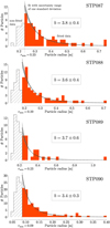 |
Fig. 7 Particle SFDs and fitted power laws of the four particle groups (Fig. 4). |
| In the text | |
|
Fig. 8 South-centered QuACK-map of the average nucleus illumination received over a whole comet day at the time of sequence STP088 (December 26, 2015). The intensity is measured in units of the average illumination at 1 AU from the Sun at the equator of the Earth over one Earth-day during equinox. The orange shapes and lines indicate the mean values within the suspected source regions. |
| In the text | |
|
Fig. 9 South-centered QuACK-maps of the average surface illumination received during the respective observational periods of the four sequences. The intensity units are the same as in Fig. 8. The mean values within the suspected source regions are indicated by the orange shapes and lines, with the areas that were selected during the respective sequences highlighted in bold. The values here are generally higher than in Fig. 8 because here the illumination was averaged over time periods when the areas were mostly in sunlight, while in Fig. 8 the illumination was averaged over a whole day-and-night cycle. |
| In the text | |
|
Fig. 10 South-centered QuACK-maps of the average surface illumination received during the 2 h prior to the respective observational periods. The figure elements and intensity scale are analogous to those in Fig. 9. |
| In the text | |
|
Fig. 11 South-centered QuACK-maps of the approximate surface acceleration, as, on 67P’s nucleus. Component parallel to the facet normal on the left, radial component on the right. The mean values within the suspected source regions are also indicated. |
| In the text | |
|
Fig. 12 2D histograms of the projected radial particle velocities, υrad, as a function of particle radius (for the selected particles, see Fig. 4). Because the polynomial fits to the particle tracks also approximate the particle accelerations, instead of using values averaged over a track, the particle velocities and radii were determined for each detection of a track individually and the results were weighted by the number of detections of the respective track (residence time weighting). The histogram data thus represent the weighted number of detections, Ñdet. Also shown are the approximate escape speeds at the suspected source regions, υesc (dotted line), and the corresponding maximum fall-back fractions, ϕfb (gray area). |
| In the text | |
|
Fig. 13 2D histograms of the projected radial particle accelerations, arad, as a function of particle radius (for the selected particles, see Fig. 4). The histogram values were determined analogously to the description in Fig. 12. Also shown are the predicted surface acceleration, as (dotted line, see also Fig. 11), and two models (dashed and solid curves) of the particle acceleration, as described by Eqs. (8) and (9). The parameters for both curves are based on our gas models (see Sect. 4.5), but for the solid curve, a local gas production rate was assumed that is about five times higher. |
| In the text | |
|
Fig. A.1 Sample images from sequences STP089 and STP090. The first images of the respective sequences are on the left, the master images on the right. The ellipses in the master images mark the suspected source regions of the concentrated particle groups. All images are brightness-inverted and had their contrasts improved for better readability (continuation of Fig. 2). |
| In the text | |
|
Fig. C.1 Same particle track shown in Fig. 3 (white circles), but this time fitted with a second-, third-, and fourth-order polynomial, each extrapolated an hour back and over two and a half hours forward in time. The plots on the right show the respective derived vertical and horizontal particle velocities and accelerations at t = 0 s. |
| In the text | |
|
Fig. D.1 Properties of the three static gas solutions that we used for our dust coma models. The plots show model cross sections that slice through the suspected source regions, which are indicated by the bold dashed curves on the top left side of the nucleus. The solar directions are highlighted by the white lines. The drag coefficient plots show the results computed for global activity of 32 cm particles, which are representative for the whole relevant size range from 1 cm to 1 m. The circular artifacts in these plots, around 3 km from the nucleus, are a consequence of how the simulation domain was built (with a transition region between an inner sphere with very small cells and an outer region with much larger cells) and the low number of simulated particles. |
| In the text | |
|
Fig. D.2 Trajectory simulations of up to 150 randomly selected particles ejected from within the suspected source region of sequence STP087. |
| In the text | |
|
Fig. D.3 Trajectory simulations of up to 150 randomly selected particles ejected from within the suspected source region of sequence STP088. |
| In the text | |
|
Fig. D.4 Trajectory simulations of up to 150 randomly selected particles ejected from within the suspected source region of sequence STP089. |
| In the text | |
|
Fig. D.5 Trajectory simulations of up to 150 randomly selected particles ejected from within the suspected source region of sequence STP090. |
| In the text | |
|
Fig. D.6 Projected radial accelerations and velocities of the particles shown in Fig. D.5 (sequence STP090). As with the OSIRIS data, the values were determined by fitting third-order polynomials to the projected tracks. In each subplot, the x-axis shows the projected radial velocity in m s−1, the y-axis the projected radial acceleration in m s−2, and the color bar the number of measurements, which are again weighted by the number of measurements per respective track (residence time weighting). The three bottom left panels are blank because no particles were ejected in these instances. |
| In the text | |
|
Fig. D.7 Coma simulations for sequence STP090 as a function of the particle SFD power-law index, b, given local activity and υirit = 0.5 m s 1. |
| In the text | |
|
Fig. D.8 Coma simulations for sequence STP090 as a function of the particle SFD power-law index, b, given nonlocal activity and υinit = 0.5 m s−1. |
| In the text | |
|
Fig. D.9 Coma simulations for sequence STP090 as a function of the particle SFD power-law index, b, given global activity and υinit = 0.5 m s−1. |
| In the text | |
|
Fig. D.10 Comparison between coma simulations with different activity distributions given υinit = 0.5 m s−1, and the observed coma in the first image of sequence STP090. The image of the observed coma is the background signal that we subtracted during the preparation for the tracking procedure (see Sect. 2 and Pfeifer et al. 2022). The ellipse indicates the suspected source region. All images are brightness-inverted and had their contrasts improved individually for better reading. Because of this, the absolute intensity levels should not be compared across images, but only relative to other areas of the same image. |
| In the text | |
|
Fig. D.11 Global coma simulations for sequence STP087 as a function of the particle SFD power-law index, b, given υinit = 0.0 m s−1. |
| In the text | |
|
Fig. D.12 Global coma simulations for sequence STP087 as a function of the particle SFD power-law index, b, given υinit = 0.25 m s−1. |
| In the text | |
|
Fig. D.13 Global coma simulations for sequence STP087 as a function of the particle SFD power-law index, b, given υinit = 0.5 m s−1. |
| In the text | |
|
Fig. D.14 Comparison between global coma simulations given different initial velocities, υinit, and the observed coma in the first image of sequence STP087. The image of the observed coma is the background signal subtracted during the preparation for the tracking procedure (see Sect. 2 and Pfeifer et al. 2022). The ellipse indicates the suspected source region. All images are brightness-inverted and had their contrasts improved individually for better readability. Because of this, the absolute intensity levels should not be compared across images, but only relative to other areas of the same image. |
| In the text | |
Current usage metrics show cumulative count of Article Views (full-text article views including HTML views, PDF and ePub downloads, according to the available data) and Abstracts Views on Vision4Press platform.
Data correspond to usage on the plateform after 2015. The current usage metrics is available 48-96 hours after online publication and is updated daily on week days.
Initial download of the metrics may take a while.