| Issue |
A&A
Volume 682, February 2024
|
|
|---|---|---|
| Article Number | A74 | |
| Number of page(s) | 14 | |
| Section | Interstellar and circumstellar matter | |
| DOI | https://doi.org/10.1051/0004-6361/202348219 | |
| Published online | 06 February 2024 | |
The GUAPOS project: G31.41+0.31 Unbiased ALMA sPectral Observational Survey
IV. Phosphorus-bearing molecules and their relation to shock tracers
1
INAF – Osservatorio Astrofisico di Arcetri,
Largo E. Fermi 5,
50125
Florence,
Italy
e-mail: This email address is being protected from spambots. You need JavaScript enabled to view it.
2
Centre for Astrochemical Studies, Max-Planck-Institute for Extraterrestrial Physics,
Giessenbachstrasse 1,
85748
Garching,
Germany
3
LERMA, Observatoire de Paris, PSL Research University, CNRS, Sorbonne Université,
92190
Meudon,
France
4
INAF – Istituto di Astrofisica e Planetologia Spaziali,
Via Fosso del Cavaliere 100,
00133
Roma,
Italy
5
Centro de Astrobiología (CSIC-INTA),
Ctra Ajalvir km 4,
28850
Torrejón de Ardoz,
Madrid,
Spain
6
Institut de Ciéncies de l’Espai (ICE, CSIC),
Can Magrans s/n,
08193,
Bellaterra, Barcelona,
Spain
7
Institut d’Estudis Espacials de Catalunya (IEEC),
Barcelona,
Spain
8
Leiden Observatory, Leiden University,
PO Box 9513,
2300 RA
Leiden,
The Netherlands
9
Department of Physics and Astronomy, University College London,
Gower Street,
London
WC1E 6BT,
UK
Received:
10
October
2023
Accepted:
21
November
2023
Abstract
Context. The astrochemistry of the important biogenic element phosphorus (P) is still poorly understood, but observational evidence indicates that P-bearing molecules are likely associated with shocks.
Aims. We study P-bearing molecules and some shock tracers towards one of the chemically richest hot molecular cores, G31.41+0.31, in the framework of the project “G31.41+0.31 Unbiased ALMA sPectral Observational Survey” (GUAPOS), which is being carried out with the Atacama Large Millimeter Array (ALMA).
Methods. We observed the molecules PN, PO, SO, SO2, SiO, and SiS through their rotational lines in the spectral range 84.05– 115.91 GHz covered by the GUAPOS project.
Results. PN is clearly detected, while PO is tentatively detected. The PN emission arises from two regions southwest of the hot core peak, named regions 1 and 2 here, and is undetected or tentatively detected towards the hot core peak. The PN and SiO lines are very similar both in spatial emission morphology and spectral shape. Region 1 is partly overlapping with the hot core and is warmer than region 2, which is well separated from the hot core and located along the outflows identified in previous studies. The SO, SO2, and SiS emissions are also detected towards the PN-emitting regions 1 and 2, but arise mostly from the hot core. Moreover, the column density ratio SiO/PN remains constant in regions 1 and 2, while SO/PN, SiS/PN, and SO2/PN decrease by about an order of magnitude from region 1 to region 2, indicating that SiO and PN have a common origin even in regions with different physical conditions. The PO/PN ratio in region 2, where PO is tentatively detected, is ~0.6–0.9, which is in line with the predictions of pure shock models.
Conclusions. Our study provides robust confirmation of previous observational evidence that PN emission is tightly associated with SiO and is likely a product of shock chemistry, as the lack of a clear detection of PN towards the hot core allows us to rule out relevant formation pathways in hot gas. We propose the PN-emitting region 2 as a new astrophysical laboratory for shock-chemistry studies.
Key words: stars: formation / ISM: molecules / ISM: individual objects: G31.41+0.31
© The Authors 2024
 Open Access article, published by EDP Sciences, under the terms of the Creative Commons Attribution License (https://creativecommons.org/licenses/by/4.0), which permits unrestricted use, distribution, and reproduction in any medium, provided the original work is properly cited.
This article is published in open access under the Subscribe to Open model. This email address is being protected from spambots. You need JavaScript enabled to view it. to support open access publication.
1 Introduction
Hot molecular cores (HMCs) are the ‘cradles’ of future high-mass stars (M ≥ 8 M⊙) and rich stellar clusters, and represent the chemically richest environment in the local interstellar medium (ISM; Bisschop et al. 2007; Fontani et al. 2007; Belloche et al. 2013; Rivilla et al. 2017). Indeed, many complex (i.e. at least six atoms) astronomical molecules have been detected for the first time towards the well-known HMCs Orion-KL (Genzel & Stutzki 1989) and Sgr B2 (e.g. Bonfand et al. 2019), including complex organic ones (COMs) such as dimethyl ether, ethanol, methyl cyanide, vinyl cyanide, and many others (McGuire 2018, 2022).
Such rich chemistry is triggered by several physical processes. First, HMCs typically harbour one or more deeply embedded protostars, which heat up their surrounding molecular gas up to temperatures of T ≥ 100 K. In this warm environment, the molecules that formed in the early cold phase in the ice mantles of dust grains sublimate back into the gas phase via thermal and non-thermal desorption (e.g. Garrod et al. 2022), and gas reactions not efficient at low temperature start to proceed and form new, more complex molecules (Garrod & Herbst 2006; Bonfand et al. 2019; Gieser et al. 2019; Barger & Garrod 2020). Second, collimated jets and molecular outflows from protostars can trigger local chemistry typical of shocked gas, such as grain sputtering and non-equilibrium chemistry (Hollenback & McKee 1989; Bachiller 1996; Tychoniec et al. 2021 ). Therefore, HMCs with a well-known physical structure are excellent astronomical laboratories for studying astrochem-istry in a variety of conditions.
In this framework, the aim of the project ‘G31.41+0.31 Unbiased ALMA sPectral Observational Survey’ (GUAPOS; Mininni et al. 2020) is to observe the full 3mm spectral window accessible with the Atacama Large Millimeter Array (ALMA) towards the well-known HMC G31.41+0.31 (G31 hereafter), which is located at a heliocentric distance of 3.75 kpc (Immer et al. 2019, see Mininni et al. 2020 for a detailed description of the source). The unbiased survey allows us to observe many transitions of different species and to confirm (or discard) their detection in a robust way. The proper identification of the species and of all their transitions is also important for the robust derivation of physical parameters, such as abundances and excitation temperatures, which are needed in order to constrain chemical models. The GUAPOS project has already provided important constraints on the formation and/or destruction routes of potential prebi-otic species such as the three isomers of C2H4O2 (Mininni et al. 2020), peptide-like bond molecules (Colzi et al. 2021), and oxygen- and nitrogen-bearing COMs (Mininni et al. 2023; López-Gallifa et al. 2023). In this work, we focus our analysis on phosphorus-bearing molecules.
Phosphorus (P) is a basic ingredient for life as we know it. P-compounds are unique in their involvement in the formation of large biomolecules thanks to their extreme structural stability and functional reactivity. For these reasons, P is a crucial component – in the form of phosphate – of nucleic acids (RNA and DNA), cellular membranes (phospholipids), and adenosine triphosphate (ATP), the key molecule for energy transfer in cells (see e.g. Macía 2005; Pasek et al. 2017). Despite its low solar abundance relative to hydrogen (P/H -3 × 10⁻⁷, Asplund et al. 2009) with respect to other biogenic elements, such as C, O, and N, its abundance in living organisms is several orders of magnitude higher than the solar abundance; for example, up to P/H ~10−3 in bacteria (e.g. Fagerbakke et al. 1996). Therefore, identifying the main source and reservoir of P in space, and understanding how its compounds form and evolve, how they are transformed and/or conserved in star-forming regions, and are finally delivered to planetary systems are of huge importance in astrophysics.
P is believed to be mainly formed in massive stars by neutron capture on silicon (Si) in hydrostatic neon-burning shells in the presupernova stage (e.g. Koo et al. 2013 and references therein), and also in explosive carbon- and neon-burning layers during supernova explosions (Woosley & Weaver 1995). In the ISM, it is less depleted than previously thought based on observations of P-bearing molecules obtained in massive star-forming regions and evolved stars (Rivilla et al. 2016; Ziurys et al. 2018). Nevertheless, a handful of P-bearing molecular species (eight in total, including the tentative detection of SiP) have been detected in the ISM, and only three of them in star-forming regions, namely PO (Rivilla et al. 2016; Lefloch et al. 2016; Wurmser & Bergner 2022), PN (Ziurys 1987; Fontani et al. 2016; Rivilla et al. 2018; Bergner et al. 2022; Wurmser & Bergner 2022), and PO+ (Rivilla et al. 2022). Single-dish observations and interferometric maps of PN and PO, the P-bearing molecules that are the easiest to detect in star-forming regions (Fontani et al. 2016; Mininni et al. 2018; Rivilla et al. 2016, 2018; Bergner et al. 2022; Wurmser & Bergner 2022) and evolved stars (Agúndez et al 2007; De Beck et al. 2013; Ziurys et al. 2018), agree with the hypothesis that PN and PO are derived from a solid phosphorus carrier, which is based on their spatial association with SiO emission, a tracer of protostellar outflows and shocks (Lefloch et al. 2016; Mininni et al. 2018; Rivilla et al. 2018; Fontani et al. 2019; Bernal et al. 2021).
Although some theoretical works have begun to determine the key reactions of the chemical network surrounding phosphorus (Fernández-Ruz et al. 2023), the reactions leading to the formation of PN and (especially) PO are far from clear. For example, Rivilla et al. (2020) proposed that to justify the observed abundances, the molecules should not be directly sputtered from the grains but formed through gas-phase photochemistry induced by ultraviolet (UV) photons from the protostar in post-shocked gas. Garcia de la Concepción et al. (2021) proposed that PO can be formed from atomic P reacting with OH, a reaction that is particularly efficient in warm environments, and Jiménez-Serra et al. (2018) also proposed mechanisms involving energetic processing. Moreover, Rivilla et al. (2020) and Bergner et al. (2022) found that PN and PO emission is cospatial with low-velocity and not with high-velocity SiO and SO emission, further complicating the simple scenario of pure grain sputtering.
Here, we study the P-bearing molecules detected in GUA-POS together with other shock tracers: the silicon-bearing molecules SiO and SiS, and the sulphur-bearing species SO and SO2. Our analysis of the aforementioned sulphur- and silicon-bearing species is limited to the regions in the core where emission from phosphorus-bearing molecules is significant. The paper is structured as follows: in Sect. 2 we describe our observations and data reduction. In Sect. 3, we present our observational results, which we then discuss in Sect. 4. Conclusions and future perspectives are given in Sect. 5.
2 Observations and data reduction
Observations towards HMC G31 were made with ALMA during Cycle 5 (project 2017.1.00501.S, P.I.: M.T. Beltrán), whereby we obtained an unbiased spectral survey in Band 3 from 84.05 GHz to 115.91 GHz. The frequency resolution is 0.49 MHz, corresponding to a velocity resolution of ~1.6 km s−1 at 90 GHz. The final angular resolution is 1″.2 (~4500 au). The primary beam is ~68″ at 84 GHz and ~50″ at 115 GHz. The pointing centre of the observations is RA(J2000) = 18h47m34″.312 and Dec(J2000) = −01° 12′45″.9. The uncertainty on the flux calibration is ~5%. For more details on the data reduction (calibration, baseline subtraction, cleaning, and line identification), we refer to Mininni et al. (2020). We performed our spectral analysis, as described in Sect. 3.3, with the MAdrid Data CUBe Analysis (MADCUBA1; Martín et al. 2019) software.
3 Results
3.1 Emission morphology
3.1.1 PN, PO, and SiO
Figure 1 shows the map of PN J = 2−1 (panel a) integrated in the velocity range with emission above 3σ rms, namely 85.7– 105.8 km s−1. As reference, the systemic velocity of G31 is 96.5 km s−1. The emission morphology is extended and located mostly towards two regions, both south of the hot core peak. The emission peak of the region showing the most intense emission is offset by −1″.6, −0″.9 from the phase centre, corresponding to ~6900 au, and is labelled 1 in Fig. 1. The second region has a complex shape with multiple peaks. The main intensity peak is offset by −3″.9,−3″.3 (corresponding to ~19000 au) from the phase centre, and is labelled region 2 in Fig 1 Towards both peaks, we extracted the PN J = 2−1 spectra, which are shown in Fig. 1. The intensity of both lines is clearly above the 3σ rms level. PO is only tentatively detected towards G31, and so we do not show the integrated map here; we refer to Sect. 3.2.2 for the analysis of this tentative detection.
Figure 1 also shows the emission of SiO J = 2−1 integrated in the same velocity range as PN J = 2−1 (85.7–105.8 km s−1, panel b). The emission morphology is in very good agreement with that of PN. In particular, SiO J = 2−1 does not peak on the hot core but towards the two PN emission regions. Evidence that PN and SiO are spatially associated was already found from both single-dish studies (Mininni et al. 2018; Rivilla et al. 2018; Fontani et al. 2019; Lefloch et al. 2016) and interferomet-ric studies (Bergner et al. 2022). The maps in Fig. 1 confirm this association very clearly. The emission from PN is less extended than that from SiO, which is perhaps due to insufficient sensitivity. To quantify this difference, we first derived the contours at half maximum of the emission of PN and SiO in region 1. The contours subtend solid angles with equivalent diameters of ~3″ and ~4″, respectively, and are therefore comparable. Second, we can quantify the expected emission of PN in the envelope detected in SiO by scaling the SiO integrated intensity by the PN/SiO abundance ratio. The average SiO integrated intensity in the envelope surrounding the emission peak 1 is ~0.4 Jy km s−1. Multiplying this value by the lowest expected PN/SiO relative abundance, which is ~0.1 as we show in Sect. 4.3, the expected integrated emission of PN is ~4 × 10⁻² Jy km s−1, which is marginally higher than the 3σ rms level in the PN map, that is 3.5 × 10⁻² Jy km s−1, and is therefore consistent with a non-detection in PN.
Moreover, SiO is also detected at higher blueshifted and red-shifted velocities with respect to the velocities detected in PN. We show the integrated emission in the blue and red wings (63.5–87 km s−1 and 102–130 km s−1, respectively) in panel c of Fig. 1. PN is undetected at these high velocities. However, the remarkable agreement between PN and SiO in the velocity range in which PN emission is significant – and where SiO emission is most intense – suggests that the two molecules have a very similar emission structure.
Panel d of Fig. 1 shows maps of the high-velocity wings of the SiO J = 5−4 line published in Beltrán et al. (2018). These maps were obtained at an angular resolution of ~0.22″, which is approximately five times higher than that of the GUAPOS maps. The orientation of the six outflows in the region and the positions of their driving sources were recently improved with ALMA (~0.09″; Beltrán et al. 2022). We can see that the PN emission is entirely to the SW of the sources driving the outflows, and can be associated with four of the six flows identified in Beltrán et al. (2022) at higher angular resolution. Thus, the complex PN emission we see in both regions 1 and 2 is probably due to the superposition of several outflow lobes. The superposition also suggests that PN is mainly associated with the blueshifted SiO outflow lobes (panel d in Fig. 1). Moreover, although region 1 is associated with both redshifted and blueshifted emission, region 2 is only detected in the blueshifted emission. This could be due to the blueshifted lobes being brighter than the red ones, although there could be other reasons for this, such as inhomogeneity of the dense gas in the clump where the hot core and outflows are embedded.
The PN emission is also clearly away from the location of the hot core, and this result is consistent with what has been observed with ALMA in the young stellar objects AFGL5142 and B1 (Rivilla et al. 2020; Bergner et al. 2022). We checked whether or not some PN emission also arises from the hot core by analysing the spectrum extracted towards the 3 mm continuum (Mininni et al. 2020). The spectrum extracted from the 3 mm continuum contour surrounding the hot core (Fig. 1) is shown in Fig. 2. We chose the 3 mm continuum contour at 20σ rms to disentangle the emission of the hot core from that of the ultracompact H II region placed NE of the hot core (Mininni et al. 2020). We also show the spectrum extracted from a beam centred on the continuum intensity peak of the hot core. We detect faint emission at ~100 km s−1 and ~80 km s−1, which is away from the systemic velocity of G31, of namely 96.5 km s−1. The feature at ~100 km s−1 is unlikely to be a nearby line because no other species have been found to emit lines at the frequency of this feature in previous GUAPOS works (Mininni et al. 2020; Colzi et al. 2021; López-Gallifa et al. 2023). Moreover, this latter feature is narrower (full width at half maximum (FWHM) of ~6 km s−1) than the lines detected towards the hot core, which have a FWHM broader than 7 km s−1 (Mininni et al. 2020, 2023; Colzi et al. 2021). The hint of an absorption feature nearby (at ~90 km s−1) suggests that this could be partially self-absorbed PN. The fact that these absorption and emission features are both more prominent towards the total hot core than towards the peak could indicate that it is PN emission from the envelope, possibly associated with narrower features, and/or partially self-absorbed in the blue part of the line. However, the candidate absorption feature is too close to the noise level in both spectra, and we therefore conclude that the emission from the hot core is lacking or negligible, as also suggested in López-Gallifa et al. (2023). The feature at -80 kms−1 could be due to n-C3H7CN 325,28 − 324,23 at 93.9839 GHz and/or gGg’-(CH2OH)2 151,14 − 142,12 at 93.9818 GHz.
We stress that we identified all the lines in the full GUAPOS spectrum towards region 2, and found no lines of other identified species that could contaminate the PN J = 2−1 line. Moreover, all lines detected towards this region were identified. Towards region 1, the identification of all species is more difficult because the full spectrum is very rich in lines. However, the clean detection towards region 2 and the lack of candidate contaminating lines from other species towards the hot core (Fig. 2) makes a contamination from other lines in region 1 also unlikely. The identification of all species in regions 1 and 2, and their comparison, goes beyond the scope of this paper, and will be the subject of a forthcoming work.
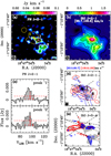 |
Fig. 1 Intensity maps of PN and SiO integrated in velocity. (a) PN J = 2−1 integrated in the range 85.7–105.8 km s−1. The white contour is the 3σ rms level of the integrated map (σ = 1.14 × 10⁻² Jy km s−1 ), while the black contours are in steps of 1σ rms. The numbered regions 1 and 2 are those used to extract the spectra of all species analysed. The synthesised beam is in the bottom-left corner. The yellow contour is the 3 mm continuum emission at 16 mJy beam−1, corresponding to 20σ rms. The yellow stars indicate the continuum sources identified by Beltrán et al. (2021). (b) Map of the intensity of SiO J = 2 − 1 integrated in the same velocity range as PN (colour scale). The PN emission regions identified in panel a are highlighted in white. Contours start at the 3σ rms level of the integrated emission (3 × 10⁻² Jy kms−1 ), and correspond to 3, 15, 30, 50, 80, and 120σ. (c) Spectra of PN J = 2 − 1 extracted from the emission peak in regions 1 (upper panel) and 2 (lower panel). The red dashed horizontal line indicates the 3σ rms level, and the vertical lines show the position in velocity of the line hyperfine components. (d) SiO J = 2 − 1 emission integrated in the velocity ranges 63.5–85.7 km s−1 (blue contours) and 105.8–130.0 km s−1 (red contours). In both cases, the starting contour is the 3σ rms level of the integrated map (1.95 × 10⁻² Jy km s−1 for the red contours, 1.62 × 10⁻² Jy km s−1 for the blue contours), and the step is 25σ. The dashed lines correspond to the six outflows identified by Beltrán et al. (2022) from SiO J = 5 − 4. The grey filled areas correspond to the PN emission regions 1 and 2 identified in panel a. (e) Same as panel d but for SiO J = 5 − 4, obtained at an angular resolution of ~0.22″ with ALMA, and already published in Beltrán et al. (2018). The integration velocity intervals are the same as in panel d. |
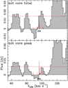 |
Fig. 2 Integrated PN J = 2−1 spectrum extracted from the hot core. The upper panel shows the spectrum extracted from the 3 mm continuum contour shown in Fig. 1. The lower panel shows the spectrum extracted from a beam around the intensity peak of the 3 mm continuum. The red vertical lines indicate the expected velocities of the hyperfine components, and their length is proportional to the relative intensity of the components. The horizontal lines illustrate the 3σ rms level. |
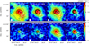 |
Fig. 3 Emission of SO, SiS, and SO2 integrated in velocity. Upper panels: velocity-integrated emission of, from left to right, SO N = 3−2, N = 2−1(2), N = 2−1(3), and N = 4−4 (see Table 1 for the spectral parameters). The integration velocity range is 85.7–105.8 km s−1 in all images to match the velocity interval where the PN emission is detected. The black contours start from the 3σ rms level of the integrated maps, which is, from left to right: 4.8 × 10⁻² Jy beam−1 km s−1; 2.5 × 10⁻² Jy beam−1 kms−1; 3.6 × 10⁻² Jy beam−1 kms−1; 2.7 × 10⁻² Jy beam−1 km s−1, and the step is of 10σ rms. The white contour corresponds to the PN integrated emission, and the numbered regions 1 and 2 are those defined in Fig. 1. The synthesised beam is illustrated in the lower-left corner. To the right of the quantum numbers, we indicate the Eup of the transition. Lower panels: same as the upper panels for the SiS J = 5−4 and J = 6−5 lines, and the |


3.1.2 SO, SiS, and SO2
Figure 3 shows the integrated intensity maps of the SO, SiS, and SO2 transitions observed in GUAPOS and detected towards the PN-emitting regions. An excitation analysis of all transitions of these species detected towards the hot core is presented in López-Gallifa et al. (2023). The SO emission arises mostly from the hot core, and shows some extended emission to the southwest, with a secondary peak towards the PN-emitting region 2 clearly visible in transitions N = 3−2 and N = 2−1(3). Therefore, overall, the bulk of the SO emission has a different morphology from that of both PN and SiO. The emission from both SiS and SO2 is also dominated by the hot core, but there is a clear secondary peak coincident with region 2. The increase in the SO, SiS, and SO2 integrated intensity towards the hot core is naturally explained if warm or hot gas-phase chemistry is boosting the formation of sulphur-bearing species. However, the SiS lines are also likely contaminated. Indeed, SiS J = 5−4 is partly blended in the hot core with a line at 90.7697 GHz, which is unidentified so far, and the SiS J = 6−5 is blended with CH3COCH3 at 108.9237 GHz and with an unidentified line detected in the hot core at 108.9216 GHz. In Sect. 3.2, we describe how such contaminations are clear closer to the hot core in region 1, and disappear in region 2.
In summary, from the integrated intensity maps of all species, the SiO emission is the most similar to the PN emission. This is further illustrated in Fig. 4, where we plot the pixel-by-pixel ratio between the PN integrated intensity map and those of SiO J = 2−1, SiS J = 5−4, SO N = 2−1(2), and  . The ratio is nearly constant (within a factor two) for SiO/PN in both regions 1 and 2, while region 1 shows an increase in the ratios SiS/PN, SO/PN, and SO2/PN by up to a factor of 10 towards the centre of the hot core. This shows that, furthermore, both PN and SiO are formed predominantly in the outflows or in their cavities, while the sulphur-bearing species are produced mostly in the hot core.
3.1.3 29SiO and 34SO
Figure 5 shows the integrated intensity maps of the lines of the less abundant but clearly detected isotopologues. Because these latter are expected to be optically thin, they should better illustrate the morphology of the molecular emission compared to the main isotopologues. Contrary to the main isotopologue, the 29SiO emission peaks on the hot core. However, this line is likely contaminated by two transitions: CH3OCHO 215,16 − 214,17 at 85.761876 GHz, and  at 85.760502 GHz. The centroid velocity of this line is expected to be displaced by about −4.5 km s−1 from 29SiO J = 2−1. Because both CH3OCHO and C2H5CN peak towards the hot core, as is the case for the other COMs detected in the region, the fact that the emission peak in the map is on the hot core is likely due to this contamination.
The emission morphologies of the 34SO lines are very similar to those of their main isotopologues: the N = 3−2 and N = 2−1(3) transitions both peak towards the hot core but have a clear secondary peak towards the PN region 2. The N = 2−1(2) line is mostly concentrated on the hot core and the secondary peak is barely visible, perhaps due to insufficient sensitivity. Therefore, the maps of the less abundant isotopologues of SO confirm the morphology of the main one, while that of SiO is different due to blending with a line arising from the hot core. However, we stress that a possible partial contamination in region 1 is also possible in the 34SO lines. In particular, the N = 2−1(2) line could be contaminated by nearby lines of CH3COOH and CH3COCH3 detected in the hot core. This would explain why the map of 34SO in this line is more concentrated towards the hot core than the others. The N = 3−2 and N = 2−1(3) could also be contaminated by nearby lines detected, but unidentified, in the hot core. In summary, the analysis of all these lines towards region 1 should therefore be regarded with caution given the strong contaminations.
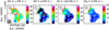 |
Fig. 4 Maps of integrated intensity ratios. The plots show the ratio between the PN integrated intensity and that of, from left to right, SiO J = 2−1. SiS J = 5−4, SO J = 2−1(2), and |

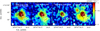 |
Fig. 5 Velocity-integrated emission of less abundant isotopologues. We show, from left to right, 29SiO J = 2−1, 34SO N = 3−2, N = 2−1(2), and N = 2−1(3). The integration velocity range is 85-101 km s−1 for 29SiO, which is the range in which PN and 29SiO are both detected. For 34SO, we used: 81–105 for the N = 3−2 line, 88–104 km s−1 for the N = 2−1(2) line, and 85.7–105.8 km s−1 for the N = 2−1(3) line. The black contours start at the 3σ rms level of the integrated intensity maps, which is, from left to right, 1.6 × 10⁻² Jy beam−1 km s−1 ; 1.8 × 10⁻² Jy beam−1 km s−1 ; 1.7 × 10⁻² Jy beam−1 km s−1 ; and 8.7 × 10⁻³ Jy beairr1 km s−1, and the step is 10σ rms. The white contour corresponds to the 3σ rms level of the integrated map of PN, and the numbered regions 1 and 2 are those defined in Fig. 1. The synthesised beam is illustrated in the bottom-left corner. |
3.2 Spectra
3.2.1 Main isotopologues
Figures 6 and 7 show the spectra of the transitions of the main isotopologues reported in Table 1, extracted at the two emitting regions of PN J = 2−1 illustrated in Fig. 1. The spectra are in brightness temperature units. The conversion from flux-density units to temperature units was performed using Eq. (1) of Fontani et al. (2021), which provides an average brightness temperature over the angular surface of each region.
The spectral profiles of SiO and PN are compared in Fig. 8, and appear similar in both regions 1 and 2. This similarity is especially apparent in the central velocity channels, while it is less clear at high velocities (≥102 km s−1, and ≤87 kms−1), where the wings detected in SiO disappear in PN. This is likely due to insufficient sensitivity in this velocity range for PN. The detection of PN in a narrower velocity range with respect to SiO has also been found through ALMA observations in the high-mass protostar AFGL5142 (Rivilla et al. 2020) and the low-mass protostar Bl-a (Bergner et al. 2022), as well as in single-dish studies (Lefloch et al. 2016; Mininni et al. 2018; Rivilla et al. 2018; Fontani et al. 2019).
Both SiS lines appear displaced (redshifted) in velocity towards region 1 with respect to PN, SiO, and SO (Fig. 6). Such a velocity shift is not seen in region 2, where the SiS velocity peak in both lines is placed very close to that of PN, SiO, and SO. We think that, in region 1, the SiS J = 5−4 line is contaminated by an unidentified line clearly detected towards the hot core at 90.7697 GHz, and the SiS J = 6−5 line is contaminated by emission of CH3COCH3 at 108.9237 GHz arising from the hot core, and by an unidentified line at 108.9216 GHz, both clearly detected towards the hot core (Mininni et al. 2023; Colzi et al. 2021).
The profiles of the SO transitions N = 2−1(2) and N = 3−2 are, overall, similar to PN in region 1 (Fig. 7), although the intensity peaks are slightly different: PN J = 2−1 and SO N = 3−2 peak at ~94 km s−1, while SO N = 2−1(2) peaks at the G31 systemic velocity, that is 96.5 km s−1. In region 2, the SO lines are narrower than those of PN and SiO, suggesting that SO could be dominated by more quiescent material, maybe surrounding the outflow lobes, towards this position rather than by shocked material.
Finally, the SO2 lines have a profile similar to that of SO in region 2, while in region 1 there are some differences: the  transition has a profile similar to that of SO, while the 31,3 − 20,2 transition shows a blended profile with the SO2 162,14 − 153,13 line (undetected in region 2) and with 13CH3OH 13−3,11 − 14−2,13 at 104.02655 GHz, which is detected towards the hot core (Mininni et al. 2023) and not towards region 2.
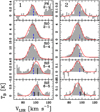 |
Fig. 6 Spectra extracted from the regions detected in PN J = 2−1. We show the transitions (from top to bottom) of PN (J = 2−1), SiO (J = 2−1 and J = 5−4) and SiS (J = 5−4 and J = 6−5). At the top of each column, we give the number of the extraction region according to the labels in Fig. 1. The blue dashed vertical lines correspond to the reference LSR velocity (96.5 km s−1; Mininni et al. 2020). The black vertical lines in the panels of the SiS J = 5−4 line correspond to an unidentified line detected in the hot core at 90.7697 GHz, and those of the J = 6−5 transition correspond to CH3COCH3 at 108.9237 GHz and to an unidentified line at 108.9216 GHz, both detected in the hot core (Mininni et al. 2023). The red curves superimposed on the lines represent the best LTE fit of the analysed molecules obtained with MAD-CUBA. For PN, we show the fit obtained fixing Tex to that of SiO, that is 26 K (see Sect. 3.3.2). |
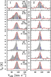 |
Fig. 7 As in Fig. 6, but showing the spectra of SO2 (J = 3−2 and J = 10 − 10) and SO (J = 2−1, J = 3−2, and J = 4−4). We keep the spectra of PN for reference in the top panels, as in Fig. 6. The black vertical lines in the spectrum of SO2 J = 3−2 are SO2 J = 16 − 15 (Table 1) and 13CH3OH J = 13 − 14 at 104.0266 GHz. |
3.2.2 Tentative detection of PO
The four lines of PO listed in Table 1 extracted from regions 1 and 2 are shown in the spectra of Fig. 9. We used MADCUBA to fit the four transitions simultaneously. The fitting method, which assumes local thermodynamic equilibrium (LTE) conditions, is fully described in Sect. 3.3.1. We have used the spectroscopic entry 047507 of the Cologne Database for Molecular Spectroscopy (CDMS), which is based on the laboratory measurements of Bailleux et al. (2002) and Kawaguchi et al. (1983), and the dipole moment determined by Kanata et al. (1988).
In region 1 (upper panel in Fig. 9), a detection of PO cannot be ruled out but it is difficult to claim due to the spectral complexity and the contamination by emission lines from other molecules (Fig. 9). In particular, the two PO transitions in the right panel of Fig. 9, namely the transitions at 109.2062 GHz and 109.2812 GHz, are blended with transitions of ethyl formate (C2H5OCHO) and ethylene glycol (aGg-CH2OH)2, respectively, as already found in source W51 (Rivilla et al. 2016). The lines contaminating the PO transitions in the left panel are not easily identifiable, as a proper determination of all contaminating species would require the study of the full GUAPOS spectrum towards this position. This goes beyond the scope of this paper and will be the subject of a forthcoming work.
In region 2 (lower panel in Fig. 9), which is less affected by nearby lines, the synthetic PO spectrum is consistent with a tentative detection. If we consider the peak intensity, the four transitions are below the 3σ rms noise, but if we consider the S/N of the line integrated intensity, the two strongest transitions, those at 108.9984 GHz and 109.2062 GHz, are consistent with a detection. The S/N of the integrated intensity can be computed from the expression ![Mathematical equation: $\int {{T_{\rm{B}}}} {\rm{d}}V/[\sigma \times \sqrt {\Delta V/FWHM} \times FWHM]$](/articles/aa/full_html/2024/02/aa48219-23/aa48219-23-eq9.png) , where ∆V is the spectral resolution in velocity. Plugging the line integrated intensity (0.51 K km s−1), the 1σ rms (0.02 K), and the FWHM obtained with MADCUBA (12 km s−1, see Table 2) into this expression, we obtain an S/N of ~6. The spectrum towards this position was smoothed in velocity by a factor 2 to increase the sensitivity. The tentative detection is supported by the fact that the emission is most likely detected towards the two lines expected to be the strongest in the quadruplet (i.e. at 108.9984 GHz and 109.2062 GHz).
, where ∆V is the spectral resolution in velocity. Plugging the line integrated intensity (0.51 K km s−1), the 1σ rms (0.02 K), and the FWHM obtained with MADCUBA (12 km s−1, see Table 2) into this expression, we obtain an S/N of ~6. The spectrum towards this position was smoothed in velocity by a factor 2 to increase the sensitivity. The tentative detection is supported by the fact that the emission is most likely detected towards the two lines expected to be the strongest in the quadruplet (i.e. at 108.9984 GHz and 109.2062 GHz).
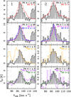 |
Fig. 8 Spectral comparison between PN, SiO, and SO. The PN J = 2−1 spectra (grey histogram) extracted from regions 1 and 2 in Fig. 1 are superimposed on SiO J = 2−1 (red histograms), SO N = 2-1(2) (magenta histograms), SO N = 3−2 (blue histograms), 29SiO J = 2-1 (orange histograms), 34SO N = 2−1(2) (purple histograms), and 34SO N = 3-2 (green histograms) extracted from the same regions. The PN line intensity scale has been appropriately multiplied to perform a consistent spectral comparison with SiO and SO. In each plot, the white vertical bars are the theoretical positions in velocity of the PN J = 2−1 hyperfine components (Table 1), with the strongest one being at the systemic velocity of 96.5 km s−1. |
3.2.3 Less abundant isotopologues
The spectra of the less abundant isotopologues, namely 29SiO, 34SO, and 33SO, extracted from regions 1 and 2 are shown in Fig. 10. We clearly detected 29SiO J = 2−1 and 34SO N = 2−1(1), 3−2, and 4−4 in both regions. The detection of 34SO N = 2−1(2) and 4−4 in region 2 is likely but difficult to confirm because it is very close to the noise level. The line profiles of the 34SO lines are overall similar in both FWHM and centroid velocity to the corresponding 32SO ones (compare Figs. 6 and 10).
The line profile of 29SiO J = 2−1 is similar to the 28SiO profile in the red wing, but this line is relatively much brighter than 28SiO in the blue wing. As already noted in Sect. 3.1.1, this excess emission is likely due to contamination from C2H5CN emission, the expected centroid velocity of which is indicated in Fig. 10.
Figure 8 shows the PN J = 2−1 line profile superimposed on the detected lines of 29SiO and 34SO. For 34SO, we use the two unblended lines N = 2−1(2) and N = 3−2. In region 2, the PN and 29SiO line profiles are very similar because29 SiO is likely less blended. The 34SO lines are very similar to PN in region 1, and are narrower in region 2. As already noted for the main isotopologue SO lines, this could be due to the fact that the SO emission is associated with more quiescent material towards this position.
We did not clearly detect any 33SO line, although towards region 1 a tentative detection of the J = 3−2 transition is possible, as shown in Fig. 10. Assuming that the line is optically thin in both less abundant isotopologues, we can verify whether or not the tentative detection in 33SO N = 3−2 is consistent with the expected line intensity: towards region 1 the 34S/33S ratio is ~5. Because the relative isotopic ratio 34S/33S is ~5.6 (Lodders 2003), the measured ratio is consistent with a tentative detection, but the 33SO line also suffers from severe blending with nearby transitions, and we therefore refrain from analysing it further.
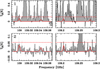 |
Fig. 9 Spectra containing the PO lines in the GUAPOS observations. Upper panel: spectrum extracted towards region 1. The red curve indicates the PO lines fitted according to the best-fit parameters in Table 2 (assuming Tex=26 K). The horizontal red dashed line corresponds to the 3σ rms level. Lower panel: same as top panel for region 2, using the fit shown in Table 2, where Tex=12 K is assumed. The observed spectra at the original frequency resolution are shown in light grey, while the spectra smoothed by a factor of 2 are shown in dark grey. |
3.3 Molecular column densities and excitation temperatures
In this section, we derive the molecular column densities, Ntot, of the analysed species. We first derive the Ntot and excitation temperature, Tex, of the molecules detected in multiple lines, namely SO, 34SO, SO2, SiS, and SiO (Sect. 3.3.1). Then, using the excitation temperature derived from these species, we compute Ntot of PN and PO (Sect. 3.3.2).
3.3.1 SO, 34SO, SO2, SiS, and SiO
The fit to the spectra of SO, 34SO, SO2, SiS, and SiO shown in Figs. 6, 7, and 10, and the derivation of the physical and spectral parameters were performed with the Spectral Line Identification and LTE Modelling (SLIM) tool of MADCUBA. Through its AUTOFIT function, SLIM produces the synthetic spectrum that best matches the data assuming LTE. The input parameters are: Tex, Ntot, radial velocity of the source (V), line FWHM, and angular size of the emission (θS). AUTOFIT assumes that V, FWHM, Tex, and θS are the same for all transitions fitted simultaneously. These input parameters have all been left free except θS, for which we can safely assume that the emission fills the telescope beam, as can be seen in Figs. 3 and 5. The results are shown in Table 2.
Let us first present the best-fit parameters of the S-bearing species. For 34So, the fit converged in region 1, leaving V, FWHM, and Ntot free, but we had to fix Tex. The best-fit Tex obtained by visual inspection is 58 K. The resulting column density in region 1 is ~1.1 × 1015 cm−2. In region 2, the fit converged, leaving all the parameters free apart from the filling factor, as explained above. The resulting Ntot is ~8 × 1013 cm−2, and Tex is 25 K. For SO, in region 1 the fit could not converge, leaving all parameters free and using all lines. We therefore did not use the N = 3−2 transition in the first instance, which has a spectral shape that suggests an excessively high optical depth. We then fitted the remaining three transitions fixing FWHM to 9 km s−1, which corresponds to the best-fit value derived from 34SO. The resulting best-fit column density and Tex are 1 × 1016 cm−2 and 60 K, respectively. In region 2, the fit converged leaving all the parameters free, and the resulting column density and Tex are ~1.2 × 1015 cm−2 and 31 K, respectively. The SO2 excitation temperature in both regions is consistent within the uncertainties with the values measured from SO (~75 K in region 1 and ~27 K in region 2), and the column densities are ~9.8 × 1015 cm−2 in region 1 and ~1.6 × 1014 cm−2 in region 2.
The fit of the lines of the Si-bearing species SiS and SiO (Fig. 6) converged leaving all parameters free except the filling factor in both regions. However, as discussed in Sect. 3.2, the SiS lines in region 1 are both strongly blended with nearby lines, some of which are from unidentified species and therefore could not be fitted simultaneously with SiS. Therefore, we only derived Ntot and Tex for region 2, where we obtain Tex ~13 K and Ntot~2.6 × 1013 cm−2. For SiO, in region 1, we derive Tex~26 K and Ntot~3.6 × 1014 cm−2, and in region 2 Tex~12 K and Ntot~1.8 × 1014 cm−2. Finally, we did not estimate the parameters for 29SiO because the line is too blended with a nearby line of C2H5CN, as discussed in Sect. 3.2.
Spectral parameters of the analysed transitions.
3.3.2 PN and PO
For PN, we cannot derive Tex from the data because we have only one transition. We therefore derived the best-fit in a range of Tex based on the minimum and maximum values obtained from the other tracers. These are 26–75 K in region 1 and 12– 30 K in region 2. The results are given in Table 2. The PN total column densities are of the order of 1013 cm−2, regardless of the region or temperature assumed. The largest PN column density is measured towards region 1 assuming Tex=75 K. We fitted the PN lines also taking the hyperfine structure into account, and derived in all cases FWHMs slightly smaller but consistent within the errors with the values obtained neglecting it.
For PO, as mentioned in Sect. 3.2.2, the PO transitions towards region 1 are significantly contaminated by brighter emission from other species. It was already noted by Rivilla et al. (2016) that the transitions at 109.2062 GHz and 109.2812 GHz are blended with transitions of ethyl formate (C2H5OCHO) and ethylene glycol (aGg-CH2OH)2, respectively. The contamination of the other two lines is less obvious and would require the analysis of the full GUAPOS spectrum towards this position, which is beyond the scope of this paper. As the presence of PO in this position cannot be confirmed, we derived an upper limit for its column density. We used the values of Tex, FWHM, and VLSR derived for PN, and used MAD CUBA to increase the value of Ntot to the maximum value that is consistent with the observing spectrum. The resulting LTE model is shown in Fig. 9, and the derived upper limit is ~1.2–1.3 (Table 2).
Regarding position 2, which is much less rich in lines, the PO transitions are not contaminated, and seem to be detected, especially the two brightest transitions. We fitted them with MADCUBA, using the same Tex, FWHM, and VLSR derived for PN. The resulting LTE fit and Ntot are shown in Fig. 9 and Table 2, respectively. We find a PO/PN ratio of ≤ 1, which is consistent with the results found in some low-mass star-forming regions (Wurmser & Bergner 2022), but is lower than the typical PO/PN ratios measured in high-mass star-forming regions (Rivilla et al. 2016, 2018) and in the comet 67P/Churyumov-Gerasimenko, where the PO/PN ratio is at least 10 (Rivilla et al. 2020).
3.3.3 Opacity of SiO and SO lines
MADCUBA estimates the line opacities as explained in Martín et al. (2019), and provides column densities already corrected for optical-depth effects. The optical depth at the line centroid velocity, τmax, computed with MADCUBA for each molecule is listed in Table 2. In case of multiple transitions, we list τmax of the line with the highest opacity. The values shown in Table 2 indicate optically thin lines in most cases except SiO, for which τmax is around 1, and SO, for which τmax is ~0.3.
For both SiO and SO lines, the opacity at line peak can also be computed from the less abundant isotopologues. Some lines of these isotopologues have the same quantum numbers as those of the main isotopologue (see Table 1). Their excitation temperatures should therefore also be comparable and the line opacity can be derived in an alternative way. If the emitting region is also the same for the two isotopologues, from the equation of radiative transfer, one can demonstrate that the ratio between the line brightness temperature of two isotopologues depends only on their relative abundance, and on the optical depth of the main isotopologue. Let us consider the case of SiO: the line intensity ratio is given by
![Mathematical equation: ${{T_{\rm{p}}^{28}} \over {T_{\rm{p}}^{29}}}\~{{1 - {{\exp }^{ - {\tau _{28}}}}} \over {1 - {{\exp }^{ - {\tau _{28}}/X[28/29]}}}},$](/articles/aa/full_html/2024/02/aa48219-23/aa48219-23-eq13.png) (1)
(1)
where  and
and  are the brightness temperatures of the two lines, τ28 is the optical depth of the main isotopologue, and X[28/29] is the 28Si/29Si relative abundance ratio. If τ28 ≪ 1, Eq. (1) states that
 ![Mathematical equation: ${{T_{\rm{p}}^{28}} \over {T_{\rm{p}}^{28}}} \sim X\left[ {{{28} \mathord{\left/ {\vphantom {{28} {29}}} \right. \kern-\nulldelimiterspace} {29}}} \right]$](/articles/aa/full_html/2024/02/aa48219-23/aa48219-23-eq16.png) , which means that the temperature ratios should be equal to the expected isotopic ratio. For SO, an equation similar to Eq. (1) is valid for the 32S/34S and 33S/34S ratios.
, which means that the temperature ratios should be equal to the expected isotopic ratio. For SO, an equation similar to Eq. (1) is valid for the 32S/34S and 33S/34S ratios.
The reference solar values for 28Si/29Si and 32SO/34SO are 19.7 (Anders & Grevesse 1989) and 22.5 (Lodders 2003), respectively. Inspection of Fig. 8 shows that, at the velocity where the 28SiO line peaks (i.e. ~94.8 kms−1), the intensity ratio between the 28SiO and the 29SiO lines is 28SiO/29 SiO~8 in region 1 and 28SiO/29SiO ~20 in region 2. This indicates that in region 2, where the isotopic ratio is very close to the solar one, both lines are likely optically thin. In region 1, the computed 28SiO/29SiO ratio gives τ28 ~ 2.35, but this is an upper limit because of the blending of 29SiO with C2H5CN. Indeed, the value computed by MADCUBA is τ28 ~ 1. In region 2 MADCUBA provides τ28 ~ 0.7, which is not consistent with optically thin lines, but is at least consistent with line opacity being smaller than that in region 1.
The32 SO/34SO ratio derived from the N = 2−1(1) line is 22 in region 2, which is consistent with optically thin emission in both lines, and 32SO/34SO~13 in region 1, which is smaller than the reference value by a factor 1.7. This ratio provides an optical depth of τ32 ~ 1.2, which is greater than the 0.34 value provided by MADCUBA, but is still consistent with moderately optically thick lines. As stated in Sect. 3.3, the N = 3−2 line is more optically thick in region 1, but it has been excluded from the fit due to its complex spectral shape that did not allow the fit to converge.
Best-fit spectral and physical parameters obtained with MADCUBA.
4 Discussion
4.1 Comparison of spatial emission between PN and shock tracers
The most direct and apparent result of this study is the similar spatial distribution of PN and the SiO J = 2−1 bulk-velocity emission. This was already found in the intermediate-/high-mass protostellar object AFGL5142 (Rivilla et al. 2020), as well as in the low-mass protostar B1-a (Bergner et al. 2022) with ALMA observations. Our findings also agree with those of these latter two works in the fact that PN does not arise from the position of the protostar(s) embedded in the hot core. The non-detection of PN towards the hot core could be explained either by insufficient atomic P to form PN, which in turn is abundant along the outflow cavities owing to grain sputtering, or to disruption of the PN molecule in the high-temperature and high-irradiation environment of the hot core. However, other species sensitive to UV photodissociation, such as methanol, are abundant towards the hot core (Mininni et al. 2023). Jiménez-Serra et al. (2018) proposed that PH3 is abundantly produced on grain surfaces via hydrogenation of P during the collapse phase. Then, upon evaporation, it is rapidly (in timescales of 104 yr) converted into PN and PO. However, both molecules are not detected clearly in the hot core, and therefore PH3 does not seem to be the main P-carrier here. The fact that PN is detected only in the shocked regions indicates that the main carrier of P is in the dust cores, where sputtering is needed to (partially or totally) destroy the grains.
The comparison between PN and SiS is less clear because the SiS emission is heavily contaminated by nearby lines close to the hot core. However, the PN line studied here has an upper level energy that is lower than those of the SiS lines (Eup ~ 7 K vs. Eup ~ 13 and ~ 18 K, respectively), and hence could be associated with (slightly) different material. If, and eventually how, the emission changes going to higher excitation lines needs to be investigated through maps of higher-J lines of PN. At present, the map of PN at the highest J at high-angular resolution is the J = 3−2 map in Bergner et al. (2022), based on observations made with ALMA towards B1-a. This map appears very similar in morphology to the PN J = 2−1 map obtained in the same work. However, the upper energy level of PN J = 3−2 is ~13.5 K, which is just a factor ≤2 higher than that of J = 2−1. It would therefore be interesting to map higher-excitation PN lines in order to check whether or not the intensity peak of the emission changes.
We also propose the PN-emitting region 2 as a new ‘hot spot’ for shocked material. This region, which is well separated from the hot core, would allow a study of the chemistry of shocked gas without the influence of the hot core, similarly to other known chemically rich, shocked protostellar spots, such as L1157–B1 (Gueth et al. 1998).
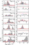 |
Fig. 10 Same as Fig. 6, but for the lines of 29SiO 7 = 2−1, ≈SO N = 2−1(2) and N = 3−2, and 34SO N = 2−1(2), N = 3−2, N = 4−4, and N = 2−1(3). The black solid vertical line in the spectrum of 29SiO 7 = 2−1 indicates the expected peak velocity of |

4.2 Comparison in velocity between PN and shock tracers
Another finding from our observations is the presence of PN only at relatively low velocities if compared with the velocities attained in the wings of the SiO and SO emission (see e.g. Fig. 6). This is also in agreement with both the high-angular-resolution studies performed towards AFGL5241 and Bl-a and the single-dish studies of Mininni et al. (2018) and Fontani et al. (2019). This could either be due to a lack of sensitivity in the high-velocity regime or to the fact that PN is only produced in relatively weak shocks. A similar behaviour is seen in young outflows (e.g. L1448-mm), where molecules such as H2S fade away rapidly for high velocities, while SiO and SO remain very bright at all velocities. One possibility could be the destruction of the onion-shell structure of dust grains where volatile species are detected at lower velocities due to the erosion of the ices and SiO and SO are also seen at high velocities because they are released from the grain cores (Jiménez-Serra et al. 2005). However, as discussed in Sect. 3.2.1, and also in Mininni et al. (2018) and Fontani et al. (2019), the fact that the line profile of PN and SiO is similar in the low(er)-velocity channels suggests that the non-detection of PN at high velocities is more likely due to the lack of sensitivity.
To quantitatively establish this, we computed the expected intensity in the wings of the SiO lines if the SiO abundance were the same as that of PN. The column-density ratio PN/SiO is <1/10 (Table 2). Figure 6 indicates that the maximum intensity in the high-velocity wings of SiO J = 2−1 is ~ 1.5 K in region 1 and ~1 K in region 2. Scaling down these values by the abundance ratio PN/SiO~l/10, which is reasonable because the emission in the wings is optically thin, one would obtain maximum intensities of 0.15 K and 0.1 K, respectively. The 1σ rms noise in the SiO J = 2−1 spectrum in region 1 is 0.1 K, and that in region 2 is 0.033 K. Thus, the intensities in the SiO wings scaled down by the PN/SiO factor would be at most 1.5 and 3 times the rms. Considering that these are upper limits, these results are consistent with a non-detection of the high-velocity wings, as we see in PN.
Concerning the PN peak velocity, in region 1, it is identical to that of SiO, and is consistent within the uncertainties with those of SO, 34SO, and SO2. In region 2, the PN peak velocity is consistent within the uncertainties with that of all the other tracers except SiO, but the difference between the two values is just ~ 1.2–1.3 km s−1, which is comparable to the velocity resolution of the observations.
4.3 Column density comparisons
Figure 11 shows the total molecular column density ratios between PN and the other species studied in this work. We plot the ratios for regions 1 and 2 calculated assuming two Tex as described in Sect. 3.3.2. The SO/PN, 34SO/PN, and S02/PN ratios are higher in region 1 by about one order of magnitude than in region 2, while the SiO/PN ratios are consistent in the two regions within the uncertainties. Because Ntot of PN remains almost constant (around 1013 cm−2) in both 1 and 2, the different ratios between the two regions arise mostly from the decrease in Ntot of SO, 34SO, and SiS by an order of magnitude. In Sect. 3.3.3, we conclude that the SiO J = 2−1 line could be affected by optical depth values higher than that provided by MADCUBA towards region 1. The upper limit on τ estimated this way is ~2.35, instead of ~0.9 obtained with MADCUBA. By correcting Ntot in Table 2 for this different T, we would obtain Ntot~6 × 1014 cm−2 towards region 1, and the SiO/PN ratios would become 66 and 24 for Tex[PN] = 12 and 60 K, respectively. Even in this case, the SiO/PN ratio for Tex[PN] = 12 would be marginally consistent with the value in region 2.
The SO/PN ratio was found to vary by orders of magnitude in the protostar AFGL5142 (Rivilla et al. 2020). In the latter source, a high-mass protostar is driving a bipolar high-velocity jet surrounded by a cavity, both clearly detected in SO. Several emission spots of PN and PO were detected along the cavity walls, but they were both undetected towards the protostar and the jet. Towards the protostar and the jet, the SO/PN ratio was of the order of 1000 or more, which is similar to the value obtained in G31 towards region 1. Along the outflow cavities, the SO/PN ratio instead drops down to ~70 – 200, which is consistent with the values we measure in region 2. As discussed in Sect. 3.3.3, the SO lines are affected by non-negligible opacities. This means that the derived total column densities of SO could be lower limits, and so the SO/PN column density ratios could be even higher. The 34SO/PN should not be affected by high optical depth effects, and even in this case the column density ratio drops by about an order of magnitude from region 1 to region 2. In summary, our study confirms that PN ans SiO are very selective tracers of outflow cavities, unlike SO and SO2.
Finally, the PO/PN ratio in region 2, where PO is tentatively detected, is ~0.6 − 0.9, and in region 1, the PO/PN upper limit is ~1.2–1.3, depending on the assumed temperature. These ratios, although in line with previous measurements on low- and highmass protostars (Rivilla et al. 2016; Lefloch et al. 2016; Wurmser & Bergner 2022), are lower than those obtained in the outflow spots of AFGL5142 (Rivilla et al. 2020), where PO/PN ≥ 1 and increases with distance from the protostar. Ratios PO/PN≤ 1 are found in the theoretical models of Jiménez-Serra et al. (2018) in the case of pure shock models, without the need for a high cosmic-ray ionisation rate, which in turn would be needed to explain PO/PN > 1.
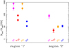 |
Fig. 11 Column density ratios between molecular species and PN. The different molecules are identified by different colours, and the measurements obtained in regions 1 and 2 are separated on the x-axis as indicated. For each molecule, we plot two values of Ntot/Ntot[PN], which correspond to the two Ntot[PN] obtained in the Tex velocity interval given in Sect. 3.3.2 (Table 2). |
5 Conclusions
In the context of the GUAPOS project, we studied P-bearing molecules towards the HMC G31 at high-angular resolution to investigate their connection with shock chemistry.
We clearly detected the PN J = 2−1 transition and several SO, SO2, SiO, and SiS rotational lines. PO lines are tentatively detected.
The integrated intensity maps indicate that the emission of PN arises from two regions, labelled regions 1 and 2 here, both southwest of the hot core peak, where four of the six outflows detected in Beltrán et al. (2022) are placed. PN is not detected towards the hot core, although region 1 is partly overlapping with it. This allows us to rule out important formation pathways in hot gas.
The PN and SiO emissions are very similar in morphology and spectral shape, both having two strong emission peaks towards regions 1 and 2, while all sulphur-bearing species emit predominantly from the hot core.
We propose that the PN-emitting region 2 is a ‘hot spot’ for shocked material well separated from the hot core, and can be used to study the chemistry of shocked gas without the influence of the hot core, similarly to other known chemically rich shocked regions powered by protostellar objects.
We derive excitation temperatures in the range of ~26–75 K in region 1, and in the range ~12–30 K in region 2. The column density ratios of all species with respect to that of PN decrease by about an order of magnitude from region 1 to region 2, except the SiO/PN ratio, which is constant within the uncertainties in both regions, further indicating a common origin of the two species.
We derive a (tentative) column density ratio PO/PN ~1 in region 2, which is in line with a pure shock model that does not need high cosmic ray ionisation rates.
An interesting follow up of our study will be to map transitions of PN at higher excitation to test whether these lines trace different (e.g. inner) material. Moreover, observing more PN lines will allow us to derive Tex for PN as well, allowing us, in turn, to compute a more accurate estimate of Ntot.
Acknowledgements
We thank the anonymous referee for their careful reading of the article and their useful comments. C.M. acknowledges funding from the European Research Council (ERC) under the European Union’s Horizon 2020 program, through the ECOGAL Synergy grant (grant ID 855130). V.M.R. has received support from the project RYC2020-029387-I funded by MCIN/AEI /10.13039/501100011033, and from the Consejo Superior de Inves-tigaciones Científicas (CSIC) and the Centro de Astrobiología (CAB) through the project 20225AT015 (Proyectos intramurales especiales del CSIC). I.J.-S. and L.C. acknowledge financial support through the Spanish grant PID2019-105552RB-C41 funded by MCIN/AEI/10.13039/501100011033. I.J.-S., L.C. and V.M.R. acknowledge also financial support through the Spanish grant PID2022-136814NBI00 funded by MCIN/AEI/10.13039/501100011033 and by “ERDF A way of making Europe”. S.V. ackowledges support from the European Research Council (ERC) Advanced grant MOPPEX 833460. This paper makes use of the following ALMA data: ADS/JAO.ALMA#2013.1.00489.S and ADS/JAO.ALMA#2017.1.00501.S.ALMA is a partnership of ESO (representing its member states), NSF (USA)and NINS (Japan), together with NRC (Canada), MOST and ASIAA (Taiwan), and KASI (Republic of Korea), in cooperation with the Republic of Chile. TheJoint ALMA Observatory is operated by ESO, AUI/NRAO and NAOJ.
References
- Agúndez, M., Cernicharo, J., & Guélin, M. 2007, ApJ, 662, L91 [CrossRef] [Google Scholar]
- Anders, E., & Grevesse, N. 1989, GeCoA, 53, 197 [NASA ADS] [CrossRef] [Google Scholar]
- Asplund, M., Grevesse, N., Sauval, A., & Jacques, S. P. 2009, ARA&A, 47, 481 [NASA ADS] [CrossRef] [Google Scholar]
- Bachiller, R. 1996, ARA&A, 34, 111 [NASA ADS] [CrossRef] [Google Scholar]
- Bailleux, S., Bogey, M., Demuynck, C., Liu, Y., & Walters, A. 2002, J. Mol. Spectrosc., 216, 465 [NASA ADS] [CrossRef] [Google Scholar]
- Barger, C. J., & Garrod, R. T. 2020, ApJ, 888, 38 [Google Scholar]
- Belloche, A., Müller, H. S. P., Menten, K. M., et al. 2013, A&A, 559, A47 [NASA ADS] [CrossRef] [EDP Sciences] [Google Scholar]
- Beltrán, M. T., Cesaroni, R., Rivilla, V. M., et al. 2018, A&A, 615, A141 [Google Scholar]
- Beltrán, M. T., Rivilla, V. M., Cesaroni, R., et al. 2021, A&A, 648, A100 [Google Scholar]
- Beltrán, M. T., Rivilla, V. M., Cesaroni, R., et al. 2022, A&A, 659, A81 [NASA ADS] [CrossRef] [EDP Sciences] [Google Scholar]
- Bergner, J. B., Burkhardt, A. M., Öberg, K. I., et al. 2022, ApJ, 927, 7 [NASA ADS] [CrossRef] [Google Scholar]
- Bernal, J. J., Koelemay, L. A., & Ziurys, L. M. 2021, ApJ, 906, 55 [NASA ADS] [CrossRef] [Google Scholar]
- Bisschop, S. E., Jørgensen, J. K., van Dishoeck, E. F., et al. 2007, A&A, 465, 913 [NASA ADS] [CrossRef] [EDP Sciences] [Google Scholar]
- Bonfand, M., Belloche, A., Garrod, R. T., et al. 2019, A&A, 628, 27 [Google Scholar]
- Colzi, L., Rivilla, V. M., Beltrán, M. T., et al. 2021, A&A, 653, 129 [Google Scholar]
- De Beck, E., Kaminski, T., Patel, N. A., et al. 2013, A&A, 558, 132 [Google Scholar]
- Endres, P., Schlemmer, S., Schilke, P., Stutzki, J., & Müller, H. S. P. 2016, J. Mol. Spectrosc., 327, 95 [NASA ADS] [CrossRef] [Google Scholar]
- Fagerbakke, K. M., Heldal, M., & Norland, S. 1996, Aquat. Microb. Ecol., 10, 15 [CrossRef] [Google Scholar]
- Fernández-Ruz, M., Jiménez-Serra, I., & Aguirre, J. 2023, ApJ, 956, 47 [CrossRef] [Google Scholar]
- Fontani, F., Pascucci, I., Caselli, P., et al. M. 2007, A&A, 470, 639 [NASA ADS] [CrossRef] [EDP Sciences] [Google Scholar]
- Fontani, F., Rivilla, V. M., Caselli, P., et al. 2016, ApJ, 822, L30 [NASA ADS] [CrossRef] [Google Scholar]
- Fontani, F., Rivilla, V. M., van der Tak, F. F. S., et al. 2019, MNRAS, 489, 4530 [CrossRef] [Google Scholar]
- Fontani, F., Barnes, A. T., Caselli, P., et al. 2021, MNRAS, 503, 4320 [NASA ADS] [CrossRef] [Google Scholar]
- García de la Concepción, J., Puzzarini, C., Barone, V., Jiménez-Serra, I., & Roncero, O. 2021, ApJ, 922, 169 [CrossRef] [Google Scholar]
- Garrod, R. T., & Herbst, E. 2006, A&A, 457, 927 [NASA ADS] [CrossRef] [EDP Sciences] [Google Scholar]
- Garrod, R. T., Jin, M., Matis, K. A., et al. 2022, ApJS, 259, 1 [NASA ADS] [CrossRef] [Google Scholar]
- Genzel, R., & Stutzki, J. 1989, ARA&A, 27, 41 [NASA ADS] [CrossRef] [Google Scholar]
- Gieser, C., Semenov, D., Beuther, H., et al. 2019, A&A, 631, 142 [Google Scholar]
- Gueth, F., Guilloteau, S., & Bachiller, R. 1998, A&A, 333, 287 [NASA ADS] [Google Scholar]
- Hollenback, D., & McKee, C. F. 1989, ApJ, 342, 306 [NASA ADS] [CrossRef] [Google Scholar]
- Immer, K., Li, J., Quiroga-Nuñez, L. H., et al. 2019, A&A, 632, A123 [NASA ADS] [CrossRef] [EDP Sciences] [Google Scholar]
- Jiménez-Serra, I., Martn-Pintado, J., Rodrǵuez-Franco, A., & Martn, S. 2005, ApJ, 627, L121 [CrossRef] [Google Scholar]
- Jiménez-Serra, I., Viti, S., Quénard, D., & Holdship, J. 2018, ApJ, 862, 128 [CrossRef] [Google Scholar]
- Kanata, H., Yamamoto, S., & Saito, M. 1988, J. Mol. Spectrosc., 131, 89 [NASA ADS] [CrossRef] [Google Scholar]
- Kawaguchi, K., Saito, S., & Hirota, E. 1983, J. Chem. Phys., 79, 629 [NASA ADS] [CrossRef] [Google Scholar]
- Koo, B.-C., Lee, Y.-H., Moon, D.-S., et al. 2013, Science, 342, 1346 [NASA ADS] [CrossRef] [Google Scholar]
- Lefloch, B., Vastel, C., Viti, S., et al. 2016, MNRAS, 462, 3937 [CrossRef] [Google Scholar]
- Lodders, K. 2003, ApJ, 591, 1220L [NASA ADS] [CrossRef] [Google Scholar]
- López-Gallifa, Á, Rivilla, V. M., Beltrán, M. T., et al. 2023, MNRAS, submitted [Google Scholar]
- Macía, E. 2005, Chem. Soc. Rev., 34, 691 [CrossRef] [Google Scholar]
- Martín, S., Martín-Pintado, J., Blanco-Sánchez, C., et al. 2019, A&A, 631, 159 [Google Scholar]
- McGuire, B. A. 2018, ApJS, 239, 17 [Google Scholar]
- McGuire, B. A. 2022, ApJS, 259, 30 [NASA ADS] [CrossRef] [Google Scholar]
- Mininni, C., Fontani, F., Rivilla, V. M., et al. 2018, MNRAS, 476, L39 [CrossRef] [Google Scholar]
- Mininni, C., Beltrán, M. T., Rivilla, V. M., et al. 2020, A&A, 644, A84 [NASA ADS] [CrossRef] [EDP Sciences] [Google Scholar]
- Mininni, C., Beltrán, M. T., Colzi, L., et al. 2023, A&A, 677, A15 [NASA ADS] [CrossRef] [EDP Sciences] [Google Scholar]
- Pasek, M. A., Gull, M., & Herschy, B. 2017, Chem. Geol., 475, 149 [NASA ADS] [CrossRef] [Google Scholar]
- Rivilla, V. M., Fontani, F., Beltrán, M. T., et al. 2016, ApJ, 826, 161 [CrossRef] [Google Scholar]
- Rivilla, V. M., Beltrán, M. T., Cesaroni, R., et al. 2017, A&A, 598, A59 [NASA ADS] [CrossRef] [EDP Sciences] [Google Scholar]
- Rivilla, V. M., Jiménez-Serra, I., Zeng, S., et al. 2018, MNRAS, 475, L30 [NASA ADS] [CrossRef] [Google Scholar]
- Rivilla, V. M., Drozdovskaya, M. N., Altwegg, K., et al. 2020, MNRAS, 492, 1180 [Google Scholar]
- Rivilla, V. M., García De La Concepción, J., Jiménez-Serra, I., et al. 2022, FrASS, 9, 9288 [NASA ADS] [Google Scholar]
- Tychoniec, L., van Dishoeck, E. F., van’t Hoff, M. L. R., et al. 2021, A&A, 655, A65 [NASA ADS] [CrossRef] [EDP Sciences] [Google Scholar]
- Wakelam, V., & Herbst, E., 2008, ApJ, 680, 371 [NASA ADS] [CrossRef] [Google Scholar]
- Woosley, S. E., & Weaver, T. A. 1995, ApJS, 101, 181 [Google Scholar]
- Wurmser, S., & Bergner, J. B. 2022, ApJ, 934, 153 [NASA ADS] [CrossRef] [Google Scholar]
- Ziurys, L. M. 1987, ApJ, 321, L81 [NASA ADS] [CrossRef] [Google Scholar]
- Ziurys, L. M., Schmidt, D. R., & Bernal, J. J. 2018, ApJ, 856, 169 [NASA ADS] [CrossRef] [Google Scholar]
MADCUBA is software developed in the Madrid Center of Astrobiology (INTA-CSIC); it enables the user to visualise and analyse single spectra and data cubes: https://cab.inta-csic.es/madcuba/
All Tables
All Figures
|
Fig. 1 Intensity maps of PN and SiO integrated in velocity. (a) PN J = 2−1 integrated in the range 85.7–105.8 km s−1. The white contour is the 3σ rms level of the integrated map (σ = 1.14 × 10⁻² Jy km s−1 ), while the black contours are in steps of 1σ rms. The numbered regions 1 and 2 are those used to extract the spectra of all species analysed. The synthesised beam is in the bottom-left corner. The yellow contour is the 3 mm continuum emission at 16 mJy beam−1, corresponding to 20σ rms. The yellow stars indicate the continuum sources identified by Beltrán et al. (2021). (b) Map of the intensity of SiO J = 2 − 1 integrated in the same velocity range as PN (colour scale). The PN emission regions identified in panel a are highlighted in white. Contours start at the 3σ rms level of the integrated emission (3 × 10⁻² Jy kms−1 ), and correspond to 3, 15, 30, 50, 80, and 120σ. (c) Spectra of PN J = 2 − 1 extracted from the emission peak in regions 1 (upper panel) and 2 (lower panel). The red dashed horizontal line indicates the 3σ rms level, and the vertical lines show the position in velocity of the line hyperfine components. (d) SiO J = 2 − 1 emission integrated in the velocity ranges 63.5–85.7 km s−1 (blue contours) and 105.8–130.0 km s−1 (red contours). In both cases, the starting contour is the 3σ rms level of the integrated map (1.95 × 10⁻² Jy km s−1 for the red contours, 1.62 × 10⁻² Jy km s−1 for the blue contours), and the step is 25σ. The dashed lines correspond to the six outflows identified by Beltrán et al. (2022) from SiO J = 5 − 4. The grey filled areas correspond to the PN emission regions 1 and 2 identified in panel a. (e) Same as panel d but for SiO J = 5 − 4, obtained at an angular resolution of ~0.22″ with ALMA, and already published in Beltrán et al. (2018). The integration velocity intervals are the same as in panel d. |
| In the text | |
|
Fig. 2 Integrated PN J = 2−1 spectrum extracted from the hot core. The upper panel shows the spectrum extracted from the 3 mm continuum contour shown in Fig. 1. The lower panel shows the spectrum extracted from a beam around the intensity peak of the 3 mm continuum. The red vertical lines indicate the expected velocities of the hyperfine components, and their length is proportional to the relative intensity of the components. The horizontal lines illustrate the 3σ rms level. |
| In the text | |
|
Fig. 3 Emission of SO, SiS, and SO2 integrated in velocity. Upper panels: velocity-integrated emission of, from left to right, SO N = 3−2, N = 2−1(2), N = 2−1(3), and N = 4−4 (see Table 1 for the spectral parameters). The integration velocity range is 85.7–105.8 km s−1 in all images to match the velocity interval where the PN emission is detected. The black contours start from the 3σ rms level of the integrated maps, which is, from left to right: 4.8 × 10⁻² Jy beam−1 km s−1; 2.5 × 10⁻² Jy beam−1 kms−1; 3.6 × 10⁻² Jy beam−1 kms−1; 2.7 × 10⁻² Jy beam−1 km s−1, and the step is of 10σ rms. The white contour corresponds to the PN integrated emission, and the numbered regions 1 and 2 are those defined in Fig. 1. The synthesised beam is illustrated in the lower-left corner. To the right of the quantum numbers, we indicate the Eup of the transition. Lower panels: same as the upper panels for the SiS J = 5−4 and J = 6−5 lines, and the |
| In the text | |
|
Fig. 4 Maps of integrated intensity ratios. The plots show the ratio between the PN integrated intensity and that of, from left to right, SiO J = 2−1. SiS J = 5−4, SO J = 2−1(2), and |
| In the text | |
|
Fig. 5 Velocity-integrated emission of less abundant isotopologues. We show, from left to right, 29SiO J = 2−1, 34SO N = 3−2, N = 2−1(2), and N = 2−1(3). The integration velocity range is 85-101 km s−1 for 29SiO, which is the range in which PN and 29SiO are both detected. For 34SO, we used: 81–105 for the N = 3−2 line, 88–104 km s−1 for the N = 2−1(2) line, and 85.7–105.8 km s−1 for the N = 2−1(3) line. The black contours start at the 3σ rms level of the integrated intensity maps, which is, from left to right, 1.6 × 10⁻² Jy beam−1 km s−1 ; 1.8 × 10⁻² Jy beam−1 km s−1 ; 1.7 × 10⁻² Jy beam−1 km s−1 ; and 8.7 × 10⁻³ Jy beairr1 km s−1, and the step is 10σ rms. The white contour corresponds to the 3σ rms level of the integrated map of PN, and the numbered regions 1 and 2 are those defined in Fig. 1. The synthesised beam is illustrated in the bottom-left corner. |
| In the text | |
|
Fig. 6 Spectra extracted from the regions detected in PN J = 2−1. We show the transitions (from top to bottom) of PN (J = 2−1), SiO (J = 2−1 and J = 5−4) and SiS (J = 5−4 and J = 6−5). At the top of each column, we give the number of the extraction region according to the labels in Fig. 1. The blue dashed vertical lines correspond to the reference LSR velocity (96.5 km s−1; Mininni et al. 2020). The black vertical lines in the panels of the SiS J = 5−4 line correspond to an unidentified line detected in the hot core at 90.7697 GHz, and those of the J = 6−5 transition correspond to CH3COCH3 at 108.9237 GHz and to an unidentified line at 108.9216 GHz, both detected in the hot core (Mininni et al. 2023). The red curves superimposed on the lines represent the best LTE fit of the analysed molecules obtained with MAD-CUBA. For PN, we show the fit obtained fixing Tex to that of SiO, that is 26 K (see Sect. 3.3.2). |
| In the text | |
|
Fig. 7 As in Fig. 6, but showing the spectra of SO2 (J = 3−2 and J = 10 − 10) and SO (J = 2−1, J = 3−2, and J = 4−4). We keep the spectra of PN for reference in the top panels, as in Fig. 6. The black vertical lines in the spectrum of SO2 J = 3−2 are SO2 J = 16 − 15 (Table 1) and 13CH3OH J = 13 − 14 at 104.0266 GHz. |
| In the text | |
|
Fig. 8 Spectral comparison between PN, SiO, and SO. The PN J = 2−1 spectra (grey histogram) extracted from regions 1 and 2 in Fig. 1 are superimposed on SiO J = 2−1 (red histograms), SO N = 2-1(2) (magenta histograms), SO N = 3−2 (blue histograms), 29SiO J = 2-1 (orange histograms), 34SO N = 2−1(2) (purple histograms), and 34SO N = 3-2 (green histograms) extracted from the same regions. The PN line intensity scale has been appropriately multiplied to perform a consistent spectral comparison with SiO and SO. In each plot, the white vertical bars are the theoretical positions in velocity of the PN J = 2−1 hyperfine components (Table 1), with the strongest one being at the systemic velocity of 96.5 km s−1. |
| In the text | |
|
Fig. 9 Spectra containing the PO lines in the GUAPOS observations. Upper panel: spectrum extracted towards region 1. The red curve indicates the PO lines fitted according to the best-fit parameters in Table 2 (assuming Tex=26 K). The horizontal red dashed line corresponds to the 3σ rms level. Lower panel: same as top panel for region 2, using the fit shown in Table 2, where Tex=12 K is assumed. The observed spectra at the original frequency resolution are shown in light grey, while the spectra smoothed by a factor of 2 are shown in dark grey. |
| In the text | |
|
Fig. 10 Same as Fig. 6, but for the lines of 29SiO 7 = 2−1, ≈SO N = 2−1(2) and N = 3−2, and 34SO N = 2−1(2), N = 3−2, N = 4−4, and N = 2−1(3). The black solid vertical line in the spectrum of 29SiO 7 = 2−1 indicates the expected peak velocity of |
| In the text | |
|
Fig. 11 Column density ratios between molecular species and PN. The different molecules are identified by different colours, and the measurements obtained in regions 1 and 2 are separated on the x-axis as indicated. For each molecule, we plot two values of Ntot/Ntot[PN], which correspond to the two Ntot[PN] obtained in the Tex velocity interval given in Sect. 3.3.2 (Table 2). |
| In the text | |
Current usage metrics show cumulative count of Article Views (full-text article views including HTML views, PDF and ePub downloads, according to the available data) and Abstracts Views on Vision4Press platform.
Data correspond to usage on the plateform after 2015. The current usage metrics is available 48-96 hours after online publication and is updated daily on week days.
Initial download of the metrics may take a while.