| Issue |
A&A
Volume 681, January 2024
|
|
|---|---|---|
| Article Number | A74 | |
| Number of page(s) | 19 | |
| Section | Interstellar and circumstellar matter | |
| DOI | https://doi.org/10.1051/0004-6361/202347710 | |
| Published online | 18 January 2024 | |
Modelling the dust emission of a filament in the Taurus molecular cloud
Department of Physics,
PO Box 64,
00014,
University of Helsinki,
Helsinki,
Finland
e-mail: This email address is being protected from spambots. You need JavaScript enabled to view it.
Received:
11
August
2023
Accepted:
20
October
2023
Abstract
Context. Dust emission is an important tool in studies of star-forming clouds as a tracer of column density. This is done indirectly via the dust evolution that is connected to the history and physical conditions of the clouds.
Aims. We examine the radiative transfer (RT) modelling of dust emission over an extended cloud region, using a filament in the Taurus molecular cloud as an example. We examine how well far-infrared (FIR) observations can be used to determine both the cloud and the dust properties.
Methods. Using different assumptions on the cloud shape, radiation field, and dust properties, we fit RT models to Herschel observations of the Taurus filament. We made further comparisons with measurements of the near-infrared extinction. The models were used to examine the degeneracies between the different cloud parameters and the dust properties.
Results. The results show a significant dependence on the assumed cloud structure and the spectral shape of the external radiation field. If these are constrained to the most likely values, the observations can be explained only if the dust FIR opacity has increased by a factor of 2–3 relative to the values in diffuse medium. However, a narrow range of FIR wavelengths provides only weak evidence of the spatial variations in dust, even in the models covering several square degrees of a molecular cloud.
Conclusions. The analysis of FIR dust emission is affected by several sources of uncertainty. Further constraints are therefore needed from observations at shorter wavelengths, especially with respect to trends in dust evolution.
Key words: ISM: clouds / infrared: ISM / submillimeter: ISM / dust, extinction / stars: formation / stars: protostars
© The Authors 2024
 Open Access article, published by EDP Sciences, under the terms of the Creative Commons Attribution License (https://creativecommons.org/licenses/by/4.0), which permits unrestricted use, distribution, and reproduction in any medium, provided the original work is properly cited.
This article is published in open access under the Subscribe to Open model. This email address is being protected from spambots. You need JavaScript enabled to view it. to support open access publication.
1 Introduction
A number of space-borne observatories have carried out observations in the near-infrared (NIR), mid-infrared (MIR), far-infrared (FIR), sub-millimetre, and millimetre wavelengths, over extended regions of the interstellar medium (ISM). These include: Planck at λ ≥ 350 µm (Tauber et al. 2010), Herschel at λ = 70–500 µm (Pilbratt et al. 2010), ISO at 2.4–250 µm (Kessler et al. 1996), AKARI at λ=1.7–180 µm (Murakami et al. 2007), Spitzer at 3.6–160 µm (Werner et al. 2004), and WISE at 3–22 µm (Wright et al. 2010). This means that many nearby clouds have been observed with the full wavelength coverage of the observable dust emission. The data have shown that the emission properties of interstellar dust are not constant at Galactic scales (Planck Collaboration XI 2014) and also change drastically between diffuse and molecular regions (Lagache et al. 1998; Cambrésy et al. 2001), even at smaller scales. One of the effects is the enhanced FIR/sub-millimetre opacity of dense molecular clouds, which is believed to be connected to the formation of ice mantles, increased grain sizes, and the formation of dust aggregates in the densest and coldest parts of the molecular clouds. A strong effect was previously observed in a filament in Taurus in Stepnik et al. (2003) and this is now known to be a common phenomenon of the densest parts of molecular clouds (Roy et al. 2013; Juvela et al. 2015b).
The changes in dust are reflected not only in the absolute opacity but also in the opacity spectral index β, which typically displays values in the range of β =1.5–2.0, depending on both the observed source and the wavelengths. Balloon-borne telescopes (Bernard et al. 1999; Dupac et al. 2003; Désert et al. 2008; Paradis et al. 2009) and the analysis of Herschel and Planck data (Paradis et al. 2010, 2012; Planck Collaboration XI 2014; Planck Collaboration Int. XXIX 2016) have revealed variations over wide sky areas. Ground-based instruments have extended the studies to millimetre wavelengths, with a resolution that is comparable to space-borne FIR data. There is evidence of the FIR spectrum getting steeper towards dense clumps and cores (Juvela et al. 2015a; Scibelli et al. 2023), but the spectrum flattens (β decreases) at longer wavelengths (Paradis et al. 2012; Planck Collaboration XI 2014). In Orion, Mason et al. (2020) found significant 3 mm and 1 cm excess over the β = 1.7 spectrum relevant to the FIR regime, which is a possible sign of the presence of extremely large grains.
Dust observations are often analysed via fits to the spectral energy distribution (SED). However, the warmest dust component within the telescope beam, including the line-of-sight (LOS) variations, has the largest effect on the SED. Therefore, the assumption of single temperature results in an overestimation |of the (mass-averaged) dust temperature (Shetty et al. 2009b; Juvela & Ysard 2012b) and the dust column densities are underestimated. With observations at more frequencies, the data can be modelled as the sum of several temperature components or a general distribution of dust temperatures (Juvela 2023). The Abel transform has been applied to the analysis of cores (Roy et al. 2014; Bracco et al. 2017), making use of the strong constraint of the spherical symmetry of the source, which is then mostly applicable for isolated cores. More generally, methods such as point process mapping (PPMAP; Marsh et al. 2015) decompose the spectrum along each line of sight into a sum of temperature components. Also, PPMAP has been applied to extended cloud regions, including cloud filaments in the Taurus molecular cloud and elsewhere Howard et al. (2019, 2021).
The simultaneous determination of the temperature and β suffers from degeneracy, which makes the results sensitive to noise and any sources of systematic errors (Shetty et al. 2009a; Veneziani et al. 2010; Juvela & Ysard 2012a). This is only partly remedied by the use of hierarchical Bayesian modelling (Kelly et al. 2012; Juvela et al. 2013), where the additional constraint comes from the assumed similarity in the (T, β) values in the observational set. With observations over a sufficiently wide wavelength range and with a sufficiently high signal-to-noise ratio (S/N), it should be possible to extract some information on the spectral index variations and even the LOS temperature variations. Both are needed for accurate optical depth estimates and better column density and mass estimates.
What the empirical SED-fitting methods lack is the requirement of physical self-consistency between the radiation field, the cloud structure, and the dust properties. Short wavelengths (from ultraviolet to NIR) determine how much energy dust absorbs and how this heating varies over the source. The energy is re-emitted at longer wavelengths, mainly in the FIR. The FIR dust properties affect the final dust temperature and, especially via β, the shape of the observed SEDs. Full self-consistency between the different wavelengths and different source regions is enforced only in a complete RT model. This should be a useful additional constraint when observations are used to study dust properties and especially their spatial variations.
The advantages of full modelling are not always self-evident. When the whole source volume is interconnected via radiation transport and the density field is complex, it is very difficult to find a model that reproduces all observations within the observational uncertainties. The predictions of a model that fits observations only approximately are naturally less reliable. In contrast, in the simple SED fits the parameters (T and possibly β) can be tuned for each pixel separately. Therefore, the observations are matched well at each position, and the main uncertainties are caused by the more naive assumptions underlying the analysis (e.g. a single temperature).
Even if a RT model does not fit the observations perfectly, the fit residuals can still provide valuable information on where the physical conditions or the dust properties differ from the model assumptions. The complexity of RT models (LOS cloud structure, spectrum and intensity of the external radiation field, positions and properties of potential embedded radiation sources, etc.) makes it difficult to cover all feasible parameter combinations. Thus, although a good fit might be reached with some RT model, the mapping of all potentially correct models (and the associated uncertainties) is hardly possible.
In this paper we construct large-scale RT models for the LDN 1506 (B212–B215) filament in the Taurus molecule cloud. The small distance (~129 pc for B215; Galli et al. 2019) and the absence of significant local heating make the region relatively easy to model. The models cover an area of 1.8 × 1.8 degrees and they are optimised to reproduce the FIR observations over the full field. The FIR emission of individual filament cross sections was already modelled in Ysard et al. (2013), suggesting clear dust evolution and increased FIR dust emissivity in the filament. Rather than trying to develop a definite model for the region and its dust property variations, we examine to what extent the FIR observations are able to constrain the dust properties. We compare models with different dust properties and investigate other factors, such as the 3D cloud density field and the external radiation field, which could confuse the evidence for dust evolution. In these models, the model parameters (apart from possible density-dependent changes in dust properties) cannot be tuned locally, so a perfect match to the observations is not to be expected. However, if the modelling were successful (and preferably without significant degeneracies), it could provide simultaneously valuable information on the dust properties, cloud mass and mass distribution, and radiation field.
The contents of the paper are the following. We present the observational data in Sect. 2 and the methods of RT modelling and employed dust models are presented in Sect.3. The results from the optimised RT models with basic dust models are presented in Sect. 4. We discuss the results in Sect. 5, where we also further investigate the dust property changes that are needed to explain the Taurus observations. The final conclusions are listed in Sect. 6.
2 Observational data
The cloud models are optimised based on 250-500 µm surface brightness observations. Measurements of NIR extinction and 160 µm emission are then used to check how well the models predict these shorter wavelength data.
2.1 Surface-brightness maps
The 250 µm, 350 µm, and 500 µm FIR surface brightness maps were all observed with the Herschel spectral and photometric imaging receiver (SPIRE) instrument, with the relative accuracy of the observations expected to be better than 2%1. The Taurus SPIRE observations were carried out as part of the Gould Belt project (PI Ph. Andre; parallel mode maps, OBS ID 1342204860 and 1342204861). The angular resolution of the observations is about 18, 26, and 37″ for the three bands in the order of increasing wavelength. For the modelling, the 250 µm and 350 µm were degraded to correspond to the Gaussian beam with the full width at half maximum (FWHM) being equal to 30″. The 500 µm data were similarly degraded to FWHM = 40″. The lower resolution relaxes the requirements for the spatial resolution of the RT models and reduces the uncertainties connected to the beam shapes. All maps were resampled onto the same 10″ pixels in galactic coordinates.
From the maps, we subtracted the background emission that was estimated as the mean value within 3.9 arcmin of the position (l,b) = (170.747 deg, −16.724deg). The details are given in Fig. 1. The data were colour-corrected for modified blackbody (MBB) spectra ∝ Bv(T) × vβ, where the temperatures were obtained from MBB fits at 40″ resolution and assuming β = 1.8. The colour corrections of the SPIRE channels are small (a couple of percent) and change only slowly as functions of temperature and spectral index. The 250 µm map is shown in Fig. 1.
We also use Herschel 160 µm maps that were observed with the photodetector array camera and spectrometer (PACS) instrument (PACS photometry maps, OBS ID 1342227304, and 1342227305). The data are convolved down to 30″ resolution and colour corrected for the same SED shape as the SPIRE channels. We assume for the PACS data a 4% uncertainty relative to the SPIRE data.
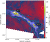 |
Fig. 1 Herschel 250 µm map of the Taurus filament. The model fits are compared mainly to the data inside the cyan contour (“filament region”), which corresponds to 10 MJy sr−1 in the background-subtracted 350 µm map. The circles labelled A-C correspond to selected small regions, in order of increasing column density, that are used in the model comparisons. The white circle shows the area used for background subtraction. |
2.2 Extinction of background stars
The NIR extinction can provide a good discriminator for different models that match the same FIR observations (Juvela et al. 2020). To estimate the NIR extinction, we use stars from the 2MASS survey (Skrutskie et al. 2006). Figure 2 shows the J-band extinction map calculated with the NICER method (Lombardi & Alves 2001) as well as the distribution of the individual stars. The area contains some 14 700 stars, 2364 of which are inside the cyan contour in Fig. 1, which we refer to as the filament region. The extinction map is made using the RV = 4 extinction law (Cardelli et al. 1989). Due to the high density of the filament region, we adopted a value above the normal ISM value of RV = 3.1, but the RV difference has a minimal effect at NIR wavelengths (Cardelli et al. 1989; Martin & Whittet 1990; Hensley & Draine 2023).
The resolution of the extinction map (2′ in Fig. 2) is restricted by the number of background stars and the stellar density decreases towards the densest regions. This results in a higher uncertainty in A (J) towards density peaks and systematic errors in regions of extinction gradients. Some or even most of the bias can be eliminated statistically (Lombardi 2009,2018). However, in the following analysis, we use the individual stars rather than the continuous extinction map. The stars probe the extinction towards discrete positions, without the uncertainty of spatial interpolation. In spite of the photometric errors and uncertainty of the intrinsic colours of the individual stars, the number of stars is sufficient for reliable comparisons with the predictions of the fitted RT models. The latter have 30″ resolution and, by construction, they do not feature any structure at scales below 10″.
3 Methods
The modelling includes the construction of the initial model setup, along with the selection of a dust model and the optimisation of the model against FIR observations. Here, the word “model” refers to the combination of the chosen density field, description of the radiation sources, and specification of the dust model.
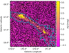 |
Fig. 2 2MASS stars (black dots) plotted on the NICER A(J) extinction map. The nominal resolution of the extinction map is 2 arcmin. |
3.1 Density field
The initial density field was constructed based on the observed 250 µm surface brightness, combined with an assumption of the line-of-sight (LOS) density profile. The absolute values or the variations in the initial mass distribution over the plane of the sky (POS) are not important because the final values will result from the model optimisation. On the other hand, the assumed LOS cloud structure is an important parameter. A larger extent means that the medium receives more radiation, leading to smaller temperature gradients and higher surface brightness per column density. We used two options for the LOS structure. The first one is a Gaussian profile that is fully determined by the FWHM of the LOS density distribution. We used three values FWHM = 0.2, 0.5, and 0.9 pc. Here FWHM = 0.2 pc is closest to the expected size of interstellar filaments, while the larger values might account for more extended cloud structures or a sheet-like geometry along the LOS direction. Alternatively, we used Plummer-type density profiles (Arzoumanian et al. 2011). Cross-sections of the column density of the main filament were fitted with the Plummer model, which were then converted to the LOS density profile under the assumption of rotational symmetry. The parameters of the Plummer fit are the central density, the size of the central flat region, and the asymptotic power-law index, p. The parameters were allowed to vary along the filament, but the p parameter was limited to the range of 1.7–3.5.
For the RT calculations, the densities were discretised onto a three-dimensional (3D) hierarchical octree grid. The modelled area is 106.7 × 106.7 arcmin in size (~3.2 square degrees) and with a pixel size of 10″, it corresponds to 640 × 640 resolution element. The octree grid has a root grid of 803 cells. With three levels of refinement, the smallest cell size thus corresponds to the 10″ pixel size and all maps of the models have the same 640 × 640 pixels as the observations. The refinement was based on volume density. By using the hierarchical discretisation, the total number of volume elements could be kept around 15 million. During the optimisation, the density field is modified based on the observed and model-predicted 350 µm surface brightness maps and the ratio in each map pixel is used to scale the densities in all cells along the same LOS. The correction changes the model column densities but does not change the original LOS density profile.
3.2 Radiation field
The dust is in the simulations heated by anisotropic background radiation. The angular distribution of the sky brightness is taken from COBE DIRBE allsky maps (Boggess et al. 1992), where the closest band is also used for frequencies outside the observed range. We only used DIRBE for the angular distribution, and the values were rescaled to match the level and spectral shape of the Mathis et al. (1983) model of the interstellar radiation field (ISRF). The strength of this external field is in RT models left as a free parameter, with the same multiplier for all frequencies. This scalar scaling parameter is optimised based on the observed and the model-predicted average surface brightness ratios Iv(250 µm)/Iv(500 µm) that are calculated over the filament region (inside the cyan contour in Fig. 1). The more diffuse regions are excluded, also because they could be subjected to different radiation fields along the LOS and could include more extended structures than in the model that is limited to a finite LOS depth.
Because the modelled region is embedded in an extended molecular cloud, we considered alternative radiation fields that have suffered AV = 0–2 magnitudes of extinction due to cloud layers outside the modelled volume. The field was attenuated according to the extinction curve of the Compiègne et al. (2011) dust model. Extinction acts to remove more energy from the shortest wavelengths. The incoming radiation was then effectively moved to longer wavelengths where it suffers less attenuation, leading to smaller temperature gradients inside the model volume. The effect is therefore qualitatively similar to the effect of a larger LOS extent of the model cloud.
Based on Planck dust optical depth maps, the LOS extinction around inside the modelled areas and outside the main filaments is AV ~ 1 mag. The scaling from 353 GHz includes large uncertainty and the visual extinction could be smaller if we assume the FIR opacity to be above the values found in diffuse regions of the Milky Way (Boulanger et al. 1996; Planck Collaboration XI 2014). Since the external layer would correspond to half of the full LOS extinction (and mutual shadowing provided by the dense filaments is quite small), the external layer is expected to correspond to less than AV = 1 mag.
The dust heating should be caused mainly by the stellar radiation field, which has some uncertainty in its level and spectral shape. Short-wavelength dust emission, such as that coming from polycyclic aromatic hydrocarbons (PAHs), could also contribute to the dust heating at high optical depths, when the short-wavelength part of the ISRF is strongly attenuated. Also this would be part of the general ISRF rather than of local origin, since the reduced abundance and excitation of PAHs reduces their emission inside dense molecular clouds. The combination of the ISRF scaling factor and the assumed external attenuation is effectively changing the balance between the heating by UV-optical and NIR-MIR radiation, whether the latter is due to PAHs or other sources. The contribution of even longer wavelengths (e.g. of the cosmic microwave background) is insignificant at the optical depths of the Taurus filaments.
We also included in some models point sources to test the effects of potential embedded sources. The luminosity of each source is left as a free parameter (reported in units of the solar luminosity) and the emission is modelled as pure blackbody radiation. The source temperature is a relevant parameter because it affects the wavelength distribution of the heating radiation and how localised the effect of each point source remains. Because of the finite resolution of the models, the temperature assigned to the sources corresponds to the escaped radiation at some 1500 au distance from the source (the minimum cell size in the models), not the intrinsic emission of an embedded (young) stellar objects. The source luminosities are optimised based on the surface brightness at 20–60″ distance of each point source. The direct LOS to the source is excluded, because that is more dependent on coarse resolution of the RT model.
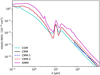 |
Fig. 3 Extinction curves of the adopted dust models. Below 70 µm the CMM-1 and CMM-2 variants are identical to CMM. |
3.3 Dust models
One of the main goals of the paper is to compare how well observations can be matched with different assumptions of the dust properties. We used three basic dust models: the Compiègne et al. (2011) model (COM, hereafter), as well as the core–mantle–mantle grains (CMM) and aggregates with ice mantles (AMMI) from the THEMIS dust model (Jones et al. 2013; Ysard et al. 2016). We also included two ad hoc variations of the CMM model. In CMM-1 the opacity spectral index β is artificially reduced by 0.3 units for all wavelengths λ > 70 µm, while keeping the 250 µm opacity unchanged. In CMM-2 the λ > 70 µm opacities are increased by 50%, with no change in β.
The extinction curves (optical depth per Hydrogen atom) of the dust models are shown in Fig. 3. It is worth noting that the absolute level of the extinction curve will have no effect on the quality of the FIR fits nor the predictions for the NIR extinction. It will affect on the mass estimates (the conversion from optical depth to mass including division with opacity κv). On the other hand, the ratio between the optical and NIR wavelengths (where dust absorbs energy) and the FIR wavelengths (where energy is re-emitted) is important for the FIR fits and especially for the predicted NIR extinction values.
In most runs, the same dust properties are used throughout the model volume. We test later also some models with a smooth transition from one set of dust properties at low densities to another at high densities. The transition is implemented with the help of fractional abundances
![Mathematical equation: $\chi = {1 \over 2} - {1 \over 2}\tanh \left[ {4.0 \times \left( {{{\log }_{10}}{n_{\rm{H}}} - {{\log }_{10}}{n_0}} \right)} \right].$](/articles/aa/full_html/2024/01/aa47710-23/aa47710-23-eq1.png) (1)
(1)
Thus, the model includes two dust components with fractional abundances χ and 1 − χ, where the values depend on the local volume density n(H) and the pre-selected density threshold n0(H).
3.4 Radiative transfer calculations
The radiative transfer calculations were carried out with the SOC Monte Carlo program (Juvela 2019), using the volume discretisation described in Sect. 3.1. Thanks to the use of hierarchical grids, the model resolution was in dense regions 10″, better than for the observations, while the run times were still manageable. To keep the Monte Carlo noise at ≲1% level (well below that of observations), we used ~ 107 photon packages per frequency for both the external field and each of the point sources. For point sources this is somewhat excessive, because the influence of each source is limited to a small region. SOC can handle spatial variations in the dust properties if, as described in Sect. 3.3, this is described using abundance variations for a finite number of dust components. A single RT run took between ~10 s and a couple of minutes, depending on the number of point sources and dust components. Because the analysis was limited to emission at long wavelengths, λ ≥ 160 µm, the stochastic heating (relevant only for small grains) was not solved, and the dust was assumed to be in equilibrium with the radiation field.
3.5 Modified blackbody fits
The optical depths of the RT models will be compared to the values obtained by fitting the SEDs with MBB functions. In the case of a single temperature component and optically thin emission, the optical depth is:
 (2)
(2)
where the dust temperature, Td, is obtained by fitting the multi-frequency observations with a MBB function:
 (3)
(3)
The dust opacity is here assumed to follow a power law of κv ∝ vβ. For this analysis, the surface brightness data are first convolved to the same resolution, which makes it possible to do the calculations for each map pixel separately.
Juvela (2023) discussed alternative SED fits, where the dust temperatures is assumed to follow a normal distribution and both the mean temperature and the width of this temperature distribution are free parameters. The fit was done with Markov chain Monte Carlo (MCMC) methods and the angular resolution of the maps at different frequencies was not required to be the same. However, in this paper, we use the observations at a common angular resolution, the same as in the case of the single-temperature fits.
4 Results
We present below results from the fitting of alternative models to the FIR observations of the Taurus B212-B215 (L1506) filament. Results are shown for single-dust models (Sect. 4.1), testing separately the potential effects of embedded sources (Sect. 4.2), before first experiments with spatial variations in the dust properties (Sect. 4.3).
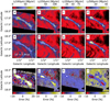 |
Fig. 4 Fit using the CMM dust model, FWHM = 0.5 pc, and AV = 0 mag. The first row of frames shows the observations, the second row the predictions of the fitted RT model, and the third row the fit residuals. The actual fit used only 250–500 µm data. The data are plotted at the resolution of the used observations, but the contours in the bottom frames show the ±4% error levels (red and blue contours, respectively) when, for clarity, the data have been smoothed to 3 arcmin resolution. |
4.1 Single-dust models
We fitted the observations with RT models with COM, CMM, CMM-1, CMM-2, and AMMI dust models (Sect. 3.3), using constant dust properties over the model volume. The optimised parameters are the column densities (adjusted pixel by pixel) and the strength of the external radiation field (a scalar parameter). Since the strength of the radiation field is optimised using the average SED in the filament region, the fit concentrates on matching the average SED shape in that area. We tested alternative models that differ regarding the LOS density profile (Sect. 3.1) and the external radiation field (Sect. 3.2).
Figure 4 presents as an example of a fit carried out with the CMM dust model, a Gaussian LOS density profile with FWHM = 0.5 pc, and no external attenuation of the ISRF. The upper frames show the observed 160–500 µm maps. The second row shows the surface brightness predictions from the RT model fitted to the 250–500 µm observations. The 160 µm map is therefore a prediction to a wavelength outside the fitted range. In the lower-left corner of the map, the RT model is extrapolated outside the SPIRE coverage in order to reduce edge effects close to the filament.
The last row of frames in Fig. 4 shows the fit residuals (percentage of the surface brightness). Because the column density is adjusted separately for each map pixel and using the observed and model-predicted 350 µm maps, the 350 µm residuals should always be close to zero. However, Fig. 4k shows one example how the fit can fail, in this case near region C (the north-eastern core). The level of the external radiation field is set based on the average signals in the filament area. However, with adopted radiation field SED and the dust properties, the model is unable to produce sufficiently high surface brightness around one position (region C). This could also happen if the core had an embedded radiation source, which is not part of the model. The positive 350 µm residuals indicate that the optimisation has at this one position increased the column density to the set upper limit (ten times the initial analytical column density estimate), and the fit in that region is incorrect.
In Fig. 4, the 250 µm and 500 µm residuals are up to a 10% level, which is thus significant compared to the relative accuracy between the SPIRE bands. At the extrapolated 160 µm wavelength the errors increase beyond 20%. The model tends to be too cold along the central filament, leading to residuals (observation minus model prediction) that are positive at 250 µm and negative at 500 µm. Because the model tries to match the average 250 µm/500 µm ratio over the whole filament region, the errors are always relative. Thus, for the optimised radiation field, the emission is too cold in the inner and too warm in the outer parts of the filament. This also means that the temperature gradients are stronger in the model than in the real cloud and the model probably has too high an optical depth at the short wavelengths responsible for the dust heating.
Figure 5 shows fits where the external radiation field is attenuated by AV = 1mag. Because the level of the radiation field is a free parameter, the effect is only to change the shape of this spectrum. As the external extinction removes energy preferentially from the short wavelengths, the model is effectively optically thinner for the remaining radiation and this should reduce the temperature variations inside the model. Compared to the previous AV = 0mag case, the fits with the CMM dust model show some improvement, and the positive 350 µm residuals cover a smaller area. The 250 µm errors are almost down to the 4% level. Interestingly, the 500 µm data, which should be less sensitive to temperature variations, show more significant variations in the residuals across the filament.
Figure 5 also shows results for two ad hoc modifications of the CMM dust model. CMM-1 has a 0.3 units lower β with no change in the 250 µm opacity and CMM-2 retains the original β but with 50% higher FIR opacity. Both CMM-1 and CMM-2 result in some improvement in the fits. The 250–500 µm fit is almost perfect with CMM-1 (with lower β), but the extrapolation to 160 µm now overestimates rather than underestimates the emission. The CMM-2 (with higher absolute FIR opacity) is close to the original CMM, but with lower errors especially at 500 µm.
The figure shows results also for two other dust models, the COM model of diffuse medium and, with its ice mantles, AMMI in principle appropriate for the densest parts of molecular clouds. Interestingly, both result in a very similar fit quality, the match to the 500 µm data being better than with CMM. Unlike the CMM model that tends to underestimate the 160 µm intensity within the filament, both COM and AMMI lead to some overestimation at this wavelength.
Instead of modifying the dust model or the radiation field, the temperature gradients can be reduced by making the cloud more extended in the LOS direction. Figure 6 shows alternative fits where the LOS density distribution corresponds FWHM of 0.2 pc, 0.5 pc, or 0.9 pc. There is a clear difference between the AV = 0mag and AV = 1mag cases, but the cloud FWHM has an even stronger effect. If the cloud is made very elongated in the LOS direction with FWHM = 0.9 pc, the fit to the 250–500 µm data is quite good, although the 160 µm emission remains overestimated.
Although interstellar filaments are expected to be narrow with FWHM ~ 0.1 pc, the FWHM parameter describes the whole cloud, where values of 0.2 pc and even 0.5 pc might still be realistic. However, the use of Plummer profiles that are derived directly from the fits to the POS filament structure (column density) should result in a better simultaneous description of both the narrow filament and the surrounding extended cloud. Figure 6 shows that this default LOS Plummer profile results in roughly similar quality of fit as the Gaussian model with FWHM = 0.5 pc. By increasing the LOS extent up to an aspect ration of 3:1, the residuals again drop to ~4% or below along the main filament.
Although the quality of the fits can be similar, different assumptions (dust, radiation field, and cloud shape) result in significantly different predictions. Figure 7 compares the NIR and FIR optical depths and the mass estimate of the fits that use different assumptions for the dust properties, the AV value of the attenuating layer, and the LOS extent of the cloud (FWHM of Gaussian density distribution). The mass estimates depend on the FIR emissivity but also indirectly on other factors that control the dust temperatures. The estimates vary by a factor of five between the COM (low FIR opacity) and AMMI (high FIR opacity) fits. However, this results directly from the different absolute dust opacities (a factor of five between AMMI and COM). The LOS cloud size is the second most important parameter, with up to 50% decrease in the mass estimates between the smallest FWHM = 0.2 pc and the largest FWHM = 0.9 pc values. The effects of the radiation field attenuation AV are only slightly smaller and are particularly clear for the more compact clouds (low FWHM). The mean optical depth τ(250 µm) varies by a factor of three and depends as much on the cloud FWHM as the dust model. The NIR and FIR optical depths are naturally correlated. There are thus similar large differences in the model-predicted τ(J) values, and direct NIR extinction measurements should be able to rule out some dust models.
Figure 8 displays a comparison of the fit quality for the models in Fig. 7. This is shown as the mean rms value of the relative error in the fitted 250–500 µm bands, which is (on average) around 5%. The plot additionally shows the rms errors of the predictions of the 160 µm surface brightness and of the J-band extinctions. The latter are calculated using the individual 2MASS stars, normalised with the formal error estimates of the AJ measurements. The SPIRE and 160 µm errors are correlated to such an extent that the addition of the 160 µm does not substantially change the conclusions reached with the SPIRE bands only. The CMM models tend to result in the worst fit. The COM and CMM-1 models give the best match to the SPIRE observations and the NIR extinctions. The CMM-2 and AMMI models are slightly worse in matching the SPIRE observations, but, compared to CMM, CMM-2 gives a much better match to NIR extinction data.
Systematic fit residuals would at first glance appear to be potential indicators of dust evolution. However, the above results show that the results are affected by multiple factors that are not related to the dust. Figure 9 shows the fit quality in region C as a function of FWHM and AV. Figure 10 is the corresponding plot for the relative residuals r (red and blue colours for positive and negative mean values of r(250 µm) – r(500 µm), respectively). As the parameters FWHM and AV are varied, the mean residual changes sign. This applies to all tested dust models and takes place over range of the (FWHM, AV) parameter space where the fit quality changes only little. Obviously, this makes it more difficult to interpret fits in terms of dust evolution. In contrast, the NIR extinction varies significantly between the dust models but is less sensitive to the FWHM and A parameters (Fig. 8).
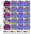 |
Fig. 5 Comparison of fit residuals in fits of single-dust models. The cloud LOS extent is FWHM = 0.5 pc and the attenuation of the external radiation field corresponds to AV = 1 mag. The rows correspond to the dust models COM, CMM, CMM-1, CMM-2, and AMMI, respectively. |
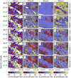 |
Fig. 6 Comparison of fit residuals for models of different cloud LOS extent. The upper three rows correspond to Gaussian LOS density profiles with FWHM equal to 0.2, 0.5, and 0.9 pc, respectively. On the fourth row the LOS profile is based on Plummer fits to the filament profile, and the last row is the same but with the cloud a factor of three longer in the LOS direction. All calculations assume an external attenuating layer of AV = 1mag. |
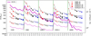 |
Fig. 7 Mass and optical depth values in selected RT models. The solid magenta line and the left axis show the estimated mass for the filament area, and the dashed magenta line and the right axis the corresponding mean optical depth τ(250 µm). The symbols show the J-band (triangles) and 250 µm (squares) optical depths (right axis) for the positions A (open symbols) and B (filled symbols). The red, black, and blue colours correspond to FWHM = 0.2, 0.5, and 0.9pc, respectively, and the small, medium, and large symbols to AV = 0, 1, and 2mag. The x-axis is also labelled according to the FWHM and AV values of the models. |
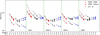 |
Fig. 8 Errors in selected model fits with the COM, CMM, CMM-1, CMM-2, and AMMI dust models. The errors are shown for the original SPIRE fit (circles) as well as for the 160 µm surface brightness (squares) and NIR extinction A(J) (triangles). For the FIR data the values are the mean relative error over the filament region. For the NIR extinction the value is the mean χ2 value that is calculated over the stars inside the filament area and using the A(J) error estimates of the individual 2MASS stars. The red, black, and blue colours correspond to FWHM = 0.2, 0.5, and 0.9 pc, respectively, and the small, medium, and large symbol sizes correspond to AV = 0, 1, and 2 mag. The x-axis is labelled according to these parameters. |
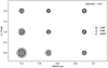 |
Fig. 9 Relative rms error for the model fits using the COM, CMM, and AMMI dust models. Errors are plotted against the FWHM (x-axis) and AV (y-axis) parameters. The data correspond to region C (cſ. Fig. 1). The diameter of the symbols is proportional to the squared error. Models with larger LOS extent and/or more extincted radiation fields tend to result in better fits. |
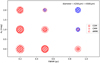 |
Fig. 10 Details are the same as in Fig. 9, but displaying the relative fit residuals (250 µm residual minus 500 µm residual) in region C. Red symbols correspond to cases where the 250 µm emission is underestimated and 500 µm emission is underestimated towards the main core. In the case of the blue symbols the situation is reversed: with larger LOS extent and large external extinction, the models overestimate rather than underestimate the dust temperature in the core. |
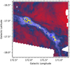 |
Fig. 11 Locations of point sources plotted on the 250 µm map of the L1506 filament. The cyan circles indicate positions of YSOs from Rebull et al. (2010), and the blue crosses the locations of hypothetical embedded sources that were added in the RT model. |
4.2 Effect of embedded point sources
The B212–B215 filament is not associated with bright stars, and YSO catalogues lists only a couple of low-luminosity sources (L < 1L⊙) that do not coincide with the cores showing the largest fit residuals. However, internal heating can significantly affect the SED of the protostellar cores relative to the surrounding filament. We tested this possibility by adding a few ad hoc point sources towards the intensity maxima in the filament of the Taurus model (Fig. 11).
The blackbody temperature of the sources was set to either 200 K or 3000 K, each run adopting the same value for all the sources. These temperatures were used to mimic different types of sources, all of which remain unresolved in our simulations. At the higher temperatures that emission is more towards the shorter wavelengths and, because of the higher optical depths, the effect should be spatially more limited. The luminosity of each source was optimised to result in zero average 250 µm residuals within 30–70″ distance of the source. The sources were places either at the exact location of the LOS density maximum or displaced by 0.2 pc along the LOS direction. The latter should lead to the effect of the sources to be spatially more extended. We note that the model cell size in dense regions is ~ 0.006 pc, much below the 0.2 pc value.
Figure 12 compares four models without point sources to the corresponding models with point sources of different temperature and LOS location. The residuals were previously seen to be largest for the smaller FWHM and AV. In these cases, the effect of point sources remains limited, partly because these models also tend to have higher optical depths (at the wavelengths relevant for dust heating). Embedded sources are not able to correct the extended positive residuals of the fits. At the same time, their effect would be locally too strong, and the observations exclude the possibility of the Taurus filament harbouring such sources (Fig. A.1). Only when the basic model already closely matches the observations, such as with FWHM = 0.5 pc and AV = 1mag, embedded sources could provide minor improvement without being very prominent in the frequency maps.
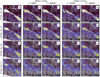 |
Fig. 12 Comparison of 250 µm fit residuals for models with hypothetical embedded sources. Each row corresponds to a combination of FWHM and AV values, as noted on the left side of the frames. Each column of frames corresponds to a different case concerning the point sources: Col. 1 is without sources, Cols. 2–3 with sources embedded at the location of the LOS density maximum, and Cols. 3–4 with sources displaced 0.2 pc along the LOS from to the density maximum. The temperatures of the point sources are given above each column of frames. |
4.3 Models with two dust components
We examined next very briefly models with spatial variations in the dust properties, using combinations of the COM, CMM, and AMMI dusts. We return in Sect. 5 to two-component models that include further modifications to the dust properties. In the RT calculations, the dust property variations are described as changes in the relative abundance of two dust species (Eq. (1)). The transition between the dust components depends on the volume density and the selected density threshold, n0. Figure 13 shows examples of how these translate to spatial distribution of the components. Because the model densities are adjusted during the model optimisation, the spatial distributions are slightly different for each dust combination and FWHM and AV values.
Figure 14 compares some two-component fits to the calculations with the single CMM dust, all with FWHM = 0.5 pc and AV = 1mag. The figure is similar to Figs. 7–8, showing the estimated masses, NIR and FIR optical depths, and the match to observations. The quality of the FIR fits (to SPIRE data and the extrapolation to 160 µm) varies only little. In the single-component tests of Fig. 8, both COM and AMMI resulted in better fits than CMM. The two-component fits are consistent with this trend: the smaller the relative abundance of the CMM dust, the better the fit. However, compared to the previous single-component models, these dust combinations provide little improvement in the FIR fits and can even increase the disagreement with the NIR extinction data.
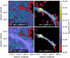 |
Fig. 13 Examples of column densities associated with the dust components in two-dust models. The plots correspond to a combination of CMM and AMMI dusts and the model parameters FWHM = 0.5 pc and AV = 1mag. The left frames show the column density associated with the dust in regions of lower volume density and the right frames the column density associated with the second dust component. The density threshold for the transition between the components is n0(H) = 1000 cm−3 in the upper and n0(H) = 3000 cm−3 in the lower frame. The cyan contour is drawn at N(H) = 1021 cm−3. |
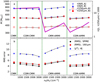 |
Fig. 14 Comparison of mass and optical depth estimates (frame a) and the quality of the fit (frame b) for models with two dust components. The results are plotted for the single-component CMM model and three dust combinations (COM-CMM, CMM-AMMI, and COM-AMMI), with density threshold n0(H1) for the transition between the two dust properties. Details of this figure are similar to Figs. 7–8, with results shown only for the case of FWHM = 0.5 pc and AV = 1mag. |
4.4 Comparison with analytical estimates
The RT modelling can serve many purposes, one of which is the study of the cloud column density structure. Column densities can be estimated also more easily using MBB fits (Sect. 3.5), but the two estimates will not be the same. An RT model gives a self-consistent description of the temperature variations within the target but does not fit the observed intensities everywhere very precisely. In contrast, MBB fits adopt a very simple model for the source (e.g. possibly a single temperature) but usually match the intensity observations better. MBB fits can use more complex assumptions but quickly suffer from the degeneracy between the fitted parameters (Juvela 2023).
Figure 15 compares optical depths with the SPIRE data (250–500 µm) at 41″ resolution. The estimates come from single-temperature MBB fits, from MBB fits with a Gaussian temperature distribution and from two selected RT models. The single-temperature calculations are taken here as the reference, although they are known to underestimate the optical depths.
The MBB fits with Gaussian temperature distribution can still be done without any priors, since they have only three free parameters (intensity, mean temperature, and width of the temperature distribution), the same as the number of observed bands. As one piece of prior information, very low temperatures Tdust < 6.5 K were excluded from the proposed temperature distributions. These fits result in higher τ values than the single-temperature fits, although the difference are only about 10% in the densest regions.
Figure 15 includes two RT models, both with FWHM = 0.5 pc and AV = 1mag. These use COM and CMM dusts for which the β values are, respectively, close to the β = 1.8 and β = 2.0 (the values also adopted for the shown MBB fits). The COM model has given a relatively good fit to the observations (Fig. 8); also, in Fig. 15 the estimates are outside the filament similar to the two MBB fits. Along the filament, the values are close to the results of the MBB fits to Gaussian temperature distributions, although the map has more noise-like fluctuations (relative to the MBB solution). The model optical depths are higher towards the densest regions, by up to 30% in region B and up to 60% in region C.
The CMM model provided a worse fit to the observations and was close to a point where it was not able to produce the observed intensity levels, especially near the C region, which can be expected to lead to higher τ values. The predicted τ values along the filament are still similar to the MBB fit with Gaussian temperature distribution solution, 5–10% above the single-temperature MBB fit. The values are higher towards the cores, by up to 40% in around region B and close to a factor of two near region C. In general, RT models should give more accurate (or more robust) estimates than simple SED fits, but only if the models also accurately match the surface brightness observations. In this case, the optical depths from the COM model might be more accurate than the predictions of the CMM model, but this also depends, for example, on the actual dust β values in the cloud. The MBB fits may look reliable, but the fact that they fit the observations to a high precision does not mean that their optical depth predictions would be accurate (Juvela 2023).
In the case of the Taurus observations mentioned above, the correct optical depths are not known. Therefore it is useful to repeat the comparison in the other direction, starting with the surface brightness maps predicted by the RT models and comparing the MBB fit results to the known optical depths of the models. The results are shown in Fig. 16, as the ratio between the MBB estimates and the now known true values. The results are qualitatively similar to the analysis of Taurus observations above. The single-temperature MBB fit underestimates the optical depth by up to ~40%, and the errors of the MBB fit with Gaussian temperature distributions is half of this and still in the same direction.
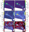 |
Fig. 15 Comparison of 250 µm optical depth estimates from MBB fits and RT models. The upper frames show the results of single-temperature MBB fits with β = 1.8 (frame a) and β = 2.0 (frame b). The second row shows the ratios between the MBB fit with a Gaussian temperature distribution and the corresponding single-temperature fit from the first row, with contours drawn at levels of ±5%. The bottom row shows the τ ratios for two RT models (FWHM = 0.5 pc, AV = 1mag) and the single-temperature MBB fits from above. The dust models are COM in frame e and CMM in frame f. |
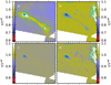 |
Fig. 16 MBB optical depth estimates calculated for synthetic observations from RT models. The uppermost frames show the results of MBB fits with a single temperature component (β = 1.8 in frame a, β = 2.0 in frame b) relative to the actual optical depths in the model. The second row shows the corresponding ratios for MBB fits with Gaussian temperature distributions. The RT models (FWHM = 0.5 pc, AV = 1mag) used either the COM (frames a and c) or the CMM dust (frames b and d). The cyan contours are drawn at the values of 0.8, 0.9, and 1.0. |
5 Discussion
The dust properties and dust evolution can be studied by comparing observations to the predictions of RT models. In this paper, we examine this using the Taurus B212-B215 (LDN 1506) filament to identify and quantify some of the factors that may affect the reliability of the conclusions derived from the modelling.
5.1 Model optimisation
In the RT modelling, we first selected the cloud shape, the dust properties, and the SED shape of the radiation field (in terms of external extinction), before optimising a set of other parameters. The optimisations were based on heuristics, which is significantly faster than blind χ2 optimisation.
The model column densities were adjusted based on the ratio of the observed and model-predicted 350 µm intensities, assuming that the surface brightness is a monotonically increasing function of the column density. Because the column density is adjusted pixel by pixel, we could expect a perfect fit at this wavelength, apart from small errors due to the model discretisation, observational artefacts, or noise at scales below the beam size. However, when the column density and radiation field were optimised, for some dust models, the intensities could be locally close to or even above what the model could produce (e.g. Fig. 4k). This also somewhat depends on the surrounding area, because of the mutual shadowing of the different parts of the cloud. Beyond the saturation point the surface brightness decreases with increasing column density. For this reason, it is important to start the model optimisation with low column densities combined with high radiation field. The problem regions can be identified from positive residuals at 350 µm (and at longer wavelengths; Fig. 6c).
If the radiation field were known, some models might be excluded already based on this saturation and observations of a single frequency. However, we included the strength of the external radiation field always as a free parameter, k(ISRF). It was updated based on the average intensity ratios Iv(250 µm)/Iv(500 µm) in the filament region, based on the knowledge that the ratio increases with increasing strength of the radiation field. The optimisation results in the correct average intensity ratio. This is similar but not exactly the same as the maximum likelihood solution (minimisation of the χ2 value summed over pixels). The distinction is not critical for the comparison of the models, especially as the fit errors are dominated by systematic and spatially correlated errors. Because the same scalar radiation field parameter applies to the whole model and also the model density field is simpler than the real cloud, a perfect fit to an extended cloud region is quite unlikely.
As described above, the optimisation always knows, based on the current solution, in which direction the free parameters are to be adjusted. Furthermore, although the number of column-density parameters was large (with over 400 000 pixels per map), these are either independent (pixels located far from each other) or strongly correlated (pixels within the same beam). This results in fast convergence and the calculations typically required only some tens of optimisation steps. Since one RT run took about 1 minute or less (down to 10 s with a single dust component and without embedded point sources), the model construction and optimisation is computationally quite feasible. The model predictions were always convolved to the resolution of the observations, which allowed us to use observational maps at different resolutions. Basic single-temperature pixel-by-pixel MBB fits can be done for small maps in a fraction of a second. However, if beam convolution is also included in the SED fitting, the run times increase and the computational advantage relative to the full RT modelling may no longer be significant (Juvela 2023).
5.2 Density fields
Compared to the POS cloud shape, the LOS structure remains poorly constrained. The LOS cloud size was also seen to have a significant effect on the dust temperature variations. In the runs with constant dust properties, the more extended models were clearly preferred for the Taurus filament. Fits to 250–500 µm data required at least FWHM = 0.5 pc, but the fits were better when the LOS cloud extent was greater (Fig. 8). Models with Plummer density profiles have given similar results, calling for larger LOS extent (e.g. with an aspect ratio of 3:1; Figs. 6q–t).
Since the fit errors were largest in areas of high column density, larger FWHM values are also needed mostly in those areas. Figure A.2 shows examples of a further test, where the FWHM is optimised as a function of the map position. A larger LOS size is indeed seen towards the cores, but the values reaching FWHM = 1.1 pc, the maximum values allowed. In the case of the Taurus filament, it is very improbable that the cloud would have such extreme elongation and just in the LOS direction. This is not necessarily the case in the analysis of isolated clumps, where the selection of bright but starless sources might be biased towards elongated sources (even filaments) that are seen along their major axis. Thus, in the absence of further information on the volume densities, the unknown cloud structure can be a significant hindrance on attempts to determine the dust properties.
In the case of the Taurus filament, the preference for longer LOS sizes could in principle be related to the source inclination, since we have so far assumed the filament to be in perpendicular to the LOS. There is some evidence that the Taurus cloud is not aligned with the plane of the sky (Roccatagliata et al. 2020; Ivanova et al. 2021), and, for example, Shimajiri et al. (2019) suggested significant 20–70 degree inclinations for the neighbouring B211/B213 filament. The inclination can increase the LOS column density without a change in the filament size perpendicular to its symmetry axis or any changes in the dust temperatures. However, when the effect of inclination was tested in practice, the fit quality changed only at ~1% level. Once the models are optimised, the LOS optical depths remain quite similar and the lower optical depth perpendicular to filament axis appear to be compensated by lower values of the external radiation field (Fig. A.3). This is similar to the conclusions of Ysard et al. (2013) regarding the effects of inclination.
One final aspect of the cloud structure that was not examined in Sect. 4 is its potential small-scale inhomogeneity. This would work in the same direction as a larger FWHM and make the model at large scales more isothermal. We tested this in the case of one model (FWHM = 0.5 pc, AV = 1mag, CMM dust) by multiplying the originally smooth density field with a Gaussian random field (standard deviation of 37%, truncated at 0) that was generated for power spectra under different power laws to compare the effects of mainly small-scale or large-scale fluctuations. However, once the model was again optimised, the differences to the original model were very small, both in terms of the fit quality and the cloud mass and ISRF estimates. Only when the density multipliers were squared (creating larger density fluctuations with a larger fraction of low-density cells), the change became noticeable, but still only at 10% level of the original fit residuals. Thus, only extreme clumpiness of the medium would alter the results.
Although the real LOS cloud extent cannot be directly measured, some limits can be extracted from line observations. Based on the densities obtained by modelling 13CO, C18O, and N2H+ observations (Pagani et al. 2010), Ysard et al. (2013) estimated for L1506C (i.e. around region B) an LOS width of at most ~0.3 pc. This is thus similar to the filament POS thickness, and models with larger FWHM (e.g. those with the 3:1 aspect ratios) appear to be unlikely in this case.
5.3 Radiation field
The radiation field was adjusted so to match the average SED shape in the filament region. This does not prevent the fits from showing spatially correlated errors at smaller spatial scales and at ~10% levels. The 250 µm and 500 µm errors are anticorre-lated, as can be expected if the dust is locally warmer or colder than in the real cloud. The residuals do not show any obvious gradients over the field, which suggests that the assumed ISRF anisotropy roughly matches the conditions in the cloud. Only the 160 µm maps might show slightly larger positive residuals on the southern side. If the ISRF were accurate outside the Taurus cloud, the part of the molecular cloud that resides between the target region and the Galactic plane could cause some shielding, which could contribute to this minor asymmetry.
The errors were always mainly correlated with the column density. The tests showed the spectral shape of the external radiation field has a clear effect on the fits, although less than the cloud FWHM. Similar to larger LOS cloud sizes, better fits were obtained by increasing the optical depth of the external attenuating cloud layer. The mechanism is also the same: once the short-wavelength photons are removed by the external layer, the model itself is heated mainly at longer wavelengths where the optical depths are lower, resulting in smaller temperature variations. The extinction was varied up to AV = 3mag but, like the 3:1 aspect ratio for the cloud shape, such high values are unlikely. In the Planck 353 GHz dust opacity map the median value over the examined area is 3.7 × 10⁻⁵. To estimate a lower limit for the LOS extinction, the 353 GHz value can be first scaled to 250 µm assuming β = 1.5, further to J-band optical depth using τ(250 µm)/τ(J) = 1.6 × 10⁻³ (Juvela et al. 2015b), and finally to visual extinction AV = 0.47mag assuming the RV = 4.0 extinction curve (Cardelli et al. 1989). On the other hand, the assumptions β = 2.0, a factor of three lower τ(250 µm)/τ(J) ratio (i.e. a value more consistent with diffuse clouds), and RV = 3.1 gives a value of 2.8mag. This applies to the full LOS extinction and gives an upper limit AV = 1.4mag for the extinction of the external layer. These are not strict limits either, since they should describe the extinction towards the main radiation sources. Due to the rest of the Taurus complex and other cloud, the extinction between the target region and the Galactic plane could be higher that between the target and the observer (or the Galactic centre).
Each fitted model gives an estimate for the ISRF strength at the boundary of the modelled volume or, for AV > 0mag, outside the assumed additional external layer. The estimates depend directly on the FIR spectral index β of the dust model and indirectly, via the dust energy balance, on the optical/FIR dust opacities. Figure 17 shows the ISRF estimates for selected models. For AV = 0mag, the values of k(ISRF) are close to one, with a scatter of some 20% and approximate agreement with the Mathis et al. (1983) ISRF model.
When AV is assumed to be larger, the k(ISRF) values are naturally larger since they describe the strength of the original field, not the field at the model boundary. According to Fig. 17, in these cases the k(ISRF) values are higher approximately by a factor eτ, where τ is the optical depth of the external layer at ~0.8 µm. The 0.8 µm optical depth thus seems to describe the effective impact of the attenuation on the dust heating. The wavelength is of course not constant but moves to larger values if the extinction is further increased. If the external attenuation is AV = 1mag, the field outside the external layer is already twice as strong as the Mathis field. Thus, in spite of the better match to the FIR observations, this makes models with AV > 1mag clearly less likely, these also being in disagreement with the direct background extinction estimates derived from Planck observations.
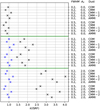 |
Fig. 17 Radiation field scaling factors k(ISRF) in case of selected single-dust models. The black crosses show the values for each combination of cloud FWHM, AV, and dust model, as listed right of the frame. In cases with AV > 0, the blue crosses show approximate values at the model boundary, if the effective attenuation is e−τ(08 µm), using the 0.8 µm optical depth of the external layer. |
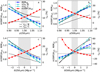 |
Fig. 18 Effects of systematic observational errors. Errors are introduced to the intensity measurements, and the frames show the effects on the filament mass M, radiation field intensity, and optical depths, τ, in sub-regions B and C. The parameters are plotted relative to those estimated with the original observations. Each frame also shows the average 250 µm residuals in the B and C regions (right y axis, dashed and continuous solid lines). The upper frames include multiplicative errors γ in the 250 µm (frame a) or 500 µm (frame b) measurements. The lower frames include additive errors δ in the same bands. The shaded regions indicate probable upper limits limits for the errors in the Taurus observations: 2% for relative calibration and (ad hoc) ±1 MJy sr−1 and ±0.5 MJy sr−1 for the 250 µm and 500 µm zero points, respectively. |
5.4 Errors in observations
Before discussing potential spatial variations of dust properties, it is worth noting that also systematic errors in the surface brightness measurements can result in variations that are correlated with the observed intensities. These could thus be misinterpreted as physical effects that would be connected to the column density and volume density variations. This is especially true for zero-point errors in the intensity measurements.
Figure 18 uses the model with FWHM = 0.5 pc, AV = 1mag, and CMM dust to illustrate the potential effects. An error is assumed to affect either the scaling or the zero point of the intensity measurements, either at 250 µm or 500 µm. The multiplicative errors (factor γ) are varied between −10% and 10%, and the additive errors in the range δ = ±3 MJy sr−1. For the SPIRE observations, the multiplicative errors should be below 2%. Additive errors could appear because of mapping artefacts (leading to errors in the difference relative to the reference regions), statistical errors in the background value derived using the reference region, or deviations from the assumption that the background SED is constant over the field. In this paper, the background subtraction was carried out using a relatively close reference region that has an absolute 350 µm surface brightness of at least 10 MJy sr−1 (Fig. 1). For the sake of discussion, the shading in Fig. 18 corresponds to ad-hoc upper limits of 1 MJy sr−1 at 250 µm and 0.5 MJy sr−1 at 500 µm for these errors.
Compared to region B, the surface brightness in region C is much closer to the level where model predictions could start to saturate, and the fits fit might behave there in an unexpected way. However, Fig. 18 shows that the behaviour is both similar and very systematic in both positions. Therefore, the estimated mass of the filament region is not unduly dependent on the fit in any single sub-region. Any errors that make the SED to appear hotter naturally decrease the mass estimates, but the effect of 2% multiplicative errors is less than 10% in the mass.
Additive errors are particularly insidious because they introduce intensity-dependent changes in the band ratios, and they can even change the sign of the residuals. In Fig. 18, this is seen only when the 500 µm measurements have zero-point errors. When the error is below δ = −0.5 MJy sr−1, the residuals in both regions B and C approach zero and they become negative for larger zero-point errors. Thus, before fit residuals can be interpreted as a sign of dust evolution, we have to be confident of sufficient absolute accuracy of the surface brightness measurements. In the Taurus data, it is unlikely that zero-point errors would explain all of the fit residuals (i.e. errors are likely to be well below 0.5 MJy sr−1 at 500 µm). However, they could still have a noticeable effect on the magnitude of the residuals, thus complicating the interpretation of the observations in terms of dust property variations. More secure conclusions could naturally be reached by investigating a set of fields, provided that all observational errors average out in a large samples.
Some zero-point errors can potentially result also from spatial variations in the SED shape of the background emission. This is not likely to be significant factor in the Taurus field, due to its high Galactic latitude (little LOS confusion) and the larger intensity contrast between the filament and the reference region. However, for compact sources this could result even in systematic effects, if the reference region is affected by limb brightening, leading to overestimation of the short-wavelength emission in the reference area compared to the target (Men’shchikov 2016).
5.5 Dust properties
Given the effects of all the other factors listed above, we consider whether something can still be said about the dust properties. In the basic single-dust models, the CMM model provided the worst fit to both the FIR data and the NIR extinction, followed by the AMMI and the COM models. The origin of the differences seems to be the same as for the other mechanisms above, lower temperature contrasts leading to better fits. First, the spectral index β is lower for COM that the other two models (∆β ~0.2), which tends to lead to higher temperatures and thus lower optical depths. Since the column densities were free parameters, the absolute level of the dust opacity is not important but the balance between the NIR and FIR opacities is. The ratios τ(250 µm)/τ(J) are for CMM and AMMI around 4.0 × 10⁻⁴ and slightly higher 4.9 × 10⁻⁴ for COM (Fig. 3). The COM models have therefore a lower optical depth at the short wavelengths, also leads to slightly a better match to the observed NIR values. The CMM-1 and CMM-2 modifications of the CMM model both go in the same direction, where the ∆β = −0.3 of CMM-1 had a larger positive effect than the 50% increase in the FIR opacity of CMM-2. The latter correspond to τ(250 µm)/τ(J) = 6 × 10⁻⁴, which is still below the value of τ(250 µm)/τ(J) = 1.6 × 10⁻³ suggested by some observations of dense clumps (Juvela et al. 2015b).
It is particularly noteworthy that all of the examined dust models have overestimated the measured NIR opacities by a large margin. This is illustrated in Fig. 19, where we plot the model values against the τ(J) estimates for the 2MASS stars. CMM is furthest and the COM and CMM-1 models closest to the observed values. The error is larger for CMM than for COM and AMMI, but the discrepancy is always significant, a factor of 2–3. This does not directly imply a similar error in the dust opacities, because the results in Fig. 8 depend in a more complex way on the model optimisation (especially on the dust temperatures).
If observations are to be fit with a single dust component, the spectral index β should be decreased or the ratio of the FIR and NIR opacities increased. Direct measurements of β are uncertain, but the typical estimates are around β = 1.8 for molecular clouds and possibly even higher in FIR observations towards dense parts of molecular clouds (Sadavoy et al. 2013; Juvela et al. 2015a, 2018; Bracco et al. 2017). The spectral index of the CMM-1 model already had a lower value of β ~ 1.7. Significantly lower β values are observed mainly at very small scales (e.g. in protostellar sources, less relevant here) and at millimetre wavelengths (Planck Collaboration Int. XVII 2014; Sadavoy et al. 2016; Mason et al. 2020). On the other hand, the dust opacity is believed to increase quite systematically from diffuse medium to molecular clouds and further to cores (Martin et al. 2012; Roy et al. 2013; Juvela et al. 2015b). In one of the earlier studies on Taurus, (Stepnik et al. 2003) concluded that the dust FIR/submm emissivity in LDN 1506 would be 3.4 times higher than in diffuse regions. Qualitatively similar conclusions were reached even for the high-latitude cloud LDN 1642, which was studied in Juvela et al. (2020). There, in addition to FIR emission and NIR extinction measurements, the need for dust with lower optical-NIR opacities was also shown by the modelling of the optical-MIR scattered light.
Based on the above, we tested a further modified dust model, CMM-3, where the FIR β was kept the same as in CMM but the FIR opacity was increased to τ(250 µm)/τ(J) = 1.2 × 10⁻³. This is a factor of three higher than in the original CMM model but still below the observed value quoted above (Juvela et al. 2015b). Figure 20 shows that CMM-3 allows for a better match to the FIR data and the 250–500 µm residuals actually do change signs between the case with FWHM = 0.2 pc and AV = 0mag and the case with FWHM = 0.5 pc and AV = 1mag. This applies even at 160 µm and the predictions for the NIR optical depth are much closer to the observations.
Thus, the observations can be explained with a model with almost the expected cloud shape and radiation field, simply by adopting the higher τ(250 µm)/τ(J) ratio. The 250–500 µm residuals are small (~10%) also outside the filament. In other words, the results do not show strong evidence for dust evolution between regions of different density. The 160 µm residuals are still positive (up to ~20%) but especially in Fig. 20b this applies to the whole field.
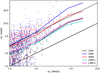 |
Fig. 19 Model predictions for τ(J) plotted against the estimates calculated for 2MASS stars. The dots represent individual stars in the filament region and the solid lines moving averages. The models correspond to AV = 1mag and FWHM = 0.5 pc and the dust models listed in the legend. The two modifications of CMM are CMM-1 (∆β = −0.3) and CMM-2 (50% increase in FIR opacity). The uncertainty of the relative zero points of the data sets is expected to be a fraction of τ(J) = 1, with little impact especially in the high-τ end of the plot. The straight black solid and dashed lines indicate, respectively, the one-to-one relationship and values higher by a factor of three. |
5.6 FIR evidence of dust evolution
Section 5.5 showed that models can match the 250–500 µm observations well, simply by assuming a high FIR-to-NIR opacity ratio (Fig. 20). Significant further fine-tuning is possible with the AV and FWHM parameters. The evidence for spatial dust property variations is not strong even at 160 µm, especially considering the potential effects of changes in the density field. Many studies have shown that higher FIR-to-NIR opacity ratios are found only in dense clouds. The lower ratios of diffuse clouds are also well constrained and correspondingly encoded in dust models (Draine 2003; Compiègne et al. 2011; Jones et al. 2013; Hensley & Draine 2023). The dust properties vary even in diffuse medium (up to 50% in the FIR-to-visual opacity ratio; Fanciullo et al. 2015) and larger changes can take place still at large scales, in the transition to molecular clouds (Roy et al. 2013; Juvela et al. 2015b; Hayashi et al. 2019). It would therefore be surprising if the dust properties remained constant over the whole area, which was well over 10 pc2 in size.
In Sect. 4.3, none of the two-component models with the COM, CMM, and AMMI dust properties resulted in significant improvement in the fits. The best combination was COM-AMMI, because those components are also individually best in fitting the FIR data. The match to NIR extinction measurements was not improved compared to the single-dust models. Therefore, a combination of different dust populations has little effect, if the dust components themselves are far from correct.
The column density was optimised for every LOS separately. This results (at least at 350 µm) to a better fit than if the densities were assumed to follow a more rigid analytical prescription. This may be particularly important when one investigates changes in the dust properties. Otherwise small differences between the assumed (analytical) density profiles and the real cloud structure could translate into artificial dust property variations in the models.
Ysard et al. (2013) used cylindrical radiative transfer models to examine the FIR observations of selected cross sections along LDN 1506 filament. With a different background subtraction, the modelling concentrated on the central ±0.2 pc part of the filament. Each cross section was optimised separately, with slightly different values of the dust and cloud parameters. A good match to both NIR extinction and FIR emission required changes in the dust properties. The models included a transition from standard diffuse-medium dust at low densities to aggregates above a sharp density threshold of ~ 1000–6000 cm−3, with a factor of ~2 increase in the 250 µm opacity. Only the low spectral index value of the adopted aggregates, β ~ 1.3, caused some problems in fitting the 500 µm observations. The FIR-to-NIR ratios of the aggregate models tested in that paper (Ossenkopf & Henning 1994; Ormel et al. 2011) were in the range of ĸ(2.2 µm/ĸ(250 µm) = 208–379. This corresponds to τ(250 µm)/τ(J) = 1 × 10⁻³ − 1.9 × 10⁻³, values that are similar or higher than in our ad-hoc CMM-3 case and in rough agreement with the earlier modelling work of Stepnik et al. (2003). At low densities, Ysard et al. (2013) adopted the dust properties from Compiègne et al. (2011). However, one can note that even the dust models developed for more diffuse Milky Way regions have significant differences in their FIR-to-NIR optical depth ratios (Guillet et al. 2018; Hensley & Draine 2023).
We used our models to attempt to find a self-consistent description for a larger cloud area. Following the above examples, we also paired a diffuse-medium dust (COM) with a dust variants with much higher FIR opacity. The other model parameters were varied in the ranges FWHM = 0.2–0.5 pc, AV = 0–1mag, and n0 = 0–3000 cm−3. For comparison, the first row of Fig. 21 shows a single-component fit with the CMM-3 dust, where the other model parameters are chosen to be between the two cases of Fig. 20 and thus nearly optimal for that dust model. The second row is a two-component fit that combines the COM and CMM-3 dusts. There is marginal improvement at 250–500 µm, and the 160 µm residuals are closer to zero, but only outside the filament. The models preferred a low value of n0, at there is little difference to the single-component fit.
We have already seen, in connection with single-dust models, that both higher FIR opacity and lower β improved the fits. On the last row of Fig. 21, COM dust is paired with another modification of CMM. The FIR opacity is increased only by a factor of two (instead of the factor of three in CMM-3) but the 250–500 µm β is also decreased to 1.72. The other parameters (FWHM, AV, n0) are the same as in the previous cases. The resulting fit to 250–500 µm is better, although the average errors were already below 5%. The main change is at 160 µm, where the average residuals are closer to zero. The lower β is compensated by higher dust temperature, which has increased the 160 µm emission from the model and reduced the average residuals closer to zero.
All three models in Fig. 20 are in good agreement with the observations of the NIR extinction. After the adoption of the CMM-3 model, the fits also appear to prefer more compact clouds shapes (FWHM < 0.5 pc) and lower cloud shielding (AV ≲ 1mag). These are both consistent with other constraints from the measurements of the volume density (this also corresponding to an approximate cylinder symmetry for the filament) and LOS extinction.
The high FIR-to-NIR opacity ratio makes the dust colder, which is compensated in the models by a stronger radiation field. These result in mass estimates that are towards the lower end of all the single-dust models in Fig. 7. All models in Fig. 20 have kISRF values close to 2, which describes the parameter describing the field outside the assumed external cloud layer. The estimated field strength also increases if β is decreased. In Fig. 20, we chose to show the model results for AV = 0.5mag, which is in best agreement with the estimates of the LOS extinction. The AV = 1mag models resulted in even slightly better fits to the 160 µm data. However, this increase in AV would also result in k(ISRF) increasing further by 0.8–1.0 units. The difference relative to models of the local ISRF may be something of a problem already for the models in Fig. 20. Also in the L 1506 models of Ysard et al. (2013), attenuated fields resulted in worse fits than the standard ISRF. However, in that case higher radiation field values were not tested. The ISRF in the solar neighbourhood is well constrained by direct and indirect observations and modelling (Mathis et al. 1983; Lehtinen & Mattila 2013; Fanciullo et al. 2015; Planck Collaboration Int. XXIX 2016; Mattila et al. 2018). It is still noteworthy that the DIRBE-observed average sky brightness is in NIR some 50% above the Mathis et al. (1983) values (Lehtinen & Mattila 1996) and the difference approaches at 5 μm a factor of two. NIR radiation is important for the dust heating in the deeper cloud layers. Nevertheless, since the Taurus filament is not likely to get significant additional heating from local radiation sources, a high k(ISRF) values of the models remain a concern.
The ratio of FIR and NIR opacities is a sensitive tracer of dust evolution. Apart from, for example, detailed spectroscopic observations of the NIR-MIR extinction curve, also dust scattering across the same wavelengths can provide useful constraints on the dust models (Lefèvre et al. 2014; Saajasto et al. 2021; Juvela et al. 2020).
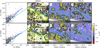 |
Fig. 20 Fits with the modified CMM-3 dust. The upper frames correspond to a FWHM = 0.2 pc and AV = 0mag model and the lower frames to a FWHM = 0.5 pc and AV = 1mag model. The leftmost frames show the model-predicted J-band optical depths against the values measured with 2MASS stars. Dots show the values for individual stars, the solid blue line is a moving average, and the straight cyan line corresponds to the one-to-one relation. The other frames show the 160, 250, and 500 µm fit residuals (rerr), where the −5% and +5% error levels are indicated with white and black contours, respectively. It is noteworthy that in the regions B and C (B212 and B215) the 250 µm and 500 µm residuals have different signs in the two models. |
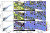 |
Fig. 21 Fits employing dust with large FIR emissivity. The left-most frames plot the model-predicted τ(J) against the observed values. The other frames show fit residuals at 160 μm, 250 μm, and 500 μm, where the −5% and +5% error levels are indicated with white and black contours, respectively. The first row shows results for a model with CMM-3 dust, and the second row for a model using a combination of COM and CMM-3. The model on the bottom row also uses two dust components, where CMM-3 is replaced with one with a lower FIR opacity (twice the value in CMM) and a lower spectral index (β ~ 1.7). The model FWHM, AV, and n0 values are listed in the second and the k(ISRF) and mass estimates of the filament region in the third frame column. |
6 Conclusions
We have modelled the FIR dust emission over an extended region of the B212-B215 filament in the Taurus molecular cloud. The goal has been to examine how the modelling results are affected by different factors and how well the dust properties can be constrained using FIR data over a limited wavelength range. We also aimed to see whether it is possible to build a self-consistent model for the larger, 16 square degree area with a large range of column densities. The fits used primarily 250–500 μm data, but the model predictions for 160 μm surface brightness and NIR extinction were also examined. We used three basic dust models from the literature (COM, CMM, and AMMI) but finally also examined what further modifications of dust opacity and opacity spectral index are needed in order to match the Taurus observations.
The use of RT modelling for the analysis of extended maps has become feasible. The three square degree maps were modelled using only ~ 15 million cells, with the run times of the individual RT runs varying between 10 s and a couple of minutes;
The models were optimised using simple heuristics for the column density and radiation field updates. This allowed for a fast convergence and the final result was usually found after some tens of iterations;
The use of the basic dust models led to small but significant differences in the FIR fit quality. Largest errors are found observed towards regions of high column density. However, the largest discrepancy was in the NIR extinction, where these models overestimated the observed NIR extinction by a factor of 2–3;
The fits are strongly affected by the assumed LOS cloud size, especially in regions of high column density and by the spectral shape of the illuminating radiation field. These effects are of similar magnitude or even larger than the differences between the tested basic dust models;
The adoption of a different dust model may cause only small changes in the fit quality and yet result in large differences in the estimates of the cloud mass (up to a factor of five for the studied models) and the radiation field intensity (up to ±30%). The mass differences are affected by the absolute values of the dust opacity, while the estimates for the optical depths varied by less than a factor of 2;
The Taurus observations could be fit, down to the 160 µm band, by adopting a dust model where the FIR opacity was increased by a factor of 2–3 (τ(250 µm)/τ(J) = (0.8 − 1.2) × 10−3). The resulting models also are in good agreement with NIR extinction observations, but require a radiation field that is twice the standard value in the solar neighbourhood;
The models are consistent with the expected dust evolution, where for example the formation of ice mantles and grain aggregates could explain the large FIR dust opacities. However, although dust can be seen to be clearly different from the normal dust in diffuse medium, the 250–500 µm or even the 160–500 µm data alone are not sufficient to unambiguously show dust property variations within the field;
The effects of dust property variations are partly degenerate with those of the poorly constrained density and radiation fields. Systematic errors in data, mainly in the zero points of the surface brightness measurements, can produce further effects that are correlated with the column density. In the case of Herschel data, the magnitude of these potential effects is small but not negligible;
The optical depths of the fitted radiative transfer models were compared to estimates from SED fitting. For the Taurus observations, single-temperature MBB fits gave expectedly the lowest values, MBB fits assuming a Gaussian temperature distribution up to 15% higher values, and radiative transfer modelling up to 50% higher values. Similar results were observed when analysing synthetic surface brightness observations from the models. However, depending on the assumed dust properties, RT models may also overestimate the optical depths and the effect can be locally significant.
To constrain the dust models further, it would be important to have multi-frequency data also on the NIR-MIR extinction and light scattering. Such observations are currently possible with the James Webb Space Telescope (JWST). As a higher mass counterpart to the Taurus filaments, the Orion molecular cloud three (OMC-3) would be a promising target, given to the clear MIR absorption seen in Spitɀer data towards its filaments (Juvela & Mannfors 2023).
Acknowledgements
M.J. acknowledges the support of the Academy of Finland Grant No. 348342.
Appendix A Additional plots
Related to the discussion in Sect. 4.2, Fig. A.1 shows the ratio of the 250 μm surface brightness maps for models with embedded radiation sources that are divided by the observed 250 μm maps. The frames corresponds to the same models as in the residual plot Fig. 12. The presence of these hypothetical embedded sources would be readily visible in the 250 μm data and they would be even more prominent at shorter wavelengths.
Figure A.2 shows additional fits, where the cloud LOS extent is optimised as a function of the sky position. These can be compared with the fits in the main paper, where the LOS FWHM value was constant over the map (e.g. Figs. 5-6). In Fig. A.2, the errors in the fitted bands (250–500 μm) are getting close to the precision of the observations. The figure quotes the [10%, 90%] percentile ranges for the pixels in the filament region. The residual maps are shown at 1 arcmin resolution, to highlight the remaining systematic errors. On the other hand, the FWHM values are ~0.5 pc or higher towards the main cores, much larger that the filament POS size and therefore unlikely to describe the real structure of the cloud.
Figure A.3 compares results for one cloud model when the filament is assumed to be either aligned with the POS or inclined by 45 degrees. The effects on the fit quality are practically invisible, and the effect on the optical depth estimates a few percentage points or less.
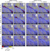 |
Fig. A.1 Ratio of modelled and observed 250 μm surface brightness maps in the case of models with ad hoc embedded sources. The models are the same as in Fig. 12. |
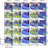 |
Fig. A.2 Examples of model fits where the LOS FWHM of the cloud is included as a free parameter. On each row, the first four frames show the 160–500 μm fit residuals, and the final frame on the right the map of the FWHM scaling (filament region only). The five rows correspond to the dust models COM, CMM, CMM-1, CMM-2, and AMMI, respectively. All calculations were done assuming AV = 1mag. The cyan contours show the outlines of the filament region, and the [10%, 90%] percentiles of the residual values are quoted in the frames (in units of percent). |
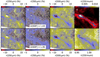 |
Fig. A.3 Comparison of model fits with different assumptions of filament inclination. The model assumes FWHM=0.5 pc and AV = 1mag and the CMM dust properties. Frames a-c show the fit residuals for the default model and frames e-g show the residuals when the filament is inclined 45 degrees with respect to POS. The corresponding scalings of the ISRF levels are given in frames b and f. Frame d shows the 250 μm optical depth for the default model, and frame h the optical depth in the inclined model relative to the default model. |
References
- Arzoumanian, D., André, P., Didelon, P., et al. 2011, A&A, 529, A6 [Google Scholar]
- Bernard, J. P., Abergel, A., Ristorcelli, I., et al. 1999, A&A, 347, 640 [NASA ADS] [Google Scholar]
- Boggess, N. W., Mather, J. C., Weiss, R., et al. 1992, ApJ, 397, 420 [Google Scholar]
- Boulanger, F., Abergel, A., Bernard, J., et al. 1996, A&A, 312, 256 [NASA ADS] [Google Scholar]
- Bracco, A., Palmeirim, P., André, P., et al. 2017, A&A, 604, A52 [NASA ADS] [CrossRef] [EDP Sciences] [Google Scholar]
- Cambrésy, L., Boulanger, F., Lagache, G., & Stepnik, B. 2001, A&A, 375, 999 [NASA ADS] [CrossRef] [EDP Sciences] [Google Scholar]
- Cardelli, J. A., Clayton, G. C., & Mathis, J. S. 1989, ApJ, 345, 245 [Google Scholar]
- Compiègne, M., Verstraete, L., Jones, A., et al. 2011, A&A, 525, A103 [Google Scholar]
- Désert, F., Macías-Pérez, J. F., Mayet, F., et al. 2008, A&A, 481, 411 [NASA ADS] [CrossRef] [EDP Sciences] [Google Scholar]
- Draine, B. T. 2003, ARA&A, 41, 241 [NASA ADS] [CrossRef] [Google Scholar]
- Dupac, X., Bernard, J., Boudet, N., et al. 2003, A&A, 404, L11 [NASA ADS] [CrossRef] [EDP Sciences] [Google Scholar]
- Fanciullo, L., Guillet, V., Aniano, G., et al. 2015, A&A, 580, A136 [NASA ADS] [CrossRef] [EDP Sciences] [Google Scholar]
- Galli, P. A. B., Loinard, L., Bouy, H., et al. 2019, A&A, 630, A137 [NASA ADS] [CrossRef] [EDP Sciences] [Google Scholar]
- Guillet, V., Fanciullo, L., Verstraete, L., et al. 2018, A&A, 610, A16 [NASA ADS] [CrossRef] [EDP Sciences] [Google Scholar]
- Hayashi, K., Mizuno, T., Fukui, Y., et al. 2019, ApJ, 884, 130 [Google Scholar]
- Hensley, B. S., & Draine, B. T. 2023, ApJ, 948, 55 [Google Scholar]
- Howard, A. D. P., Whitworth, A. P., Marsh, K. A., et al. 2019, MNRAS, 489, 962 [NASA ADS] [CrossRef] [Google Scholar]
- Howard, A. D. P., Whitworth, A. P., Griffin, M. J., Marsh, K. A., & Smith, M. W. L. 2021, MNRAS, 504, 6157 [NASA ADS] [CrossRef] [Google Scholar]
- Ivanova, A., Lallement, R., Vergely, J. L., & Hottier, C. 2021, A&A, 652, A22 [NASA ADS] [CrossRef] [EDP Sciences] [Google Scholar]
- Jones, A. P., Fanciullo, L., Köhler, M., et al. 2013, A&A, 558, A62 [NASA ADS] [CrossRef] [EDP Sciences] [Google Scholar]
- Juvela, M. 2019, A&A, 622, A79 [NASA ADS] [CrossRef] [EDP Sciences] [Google Scholar]
- Juvela, M. 2023, A&A, 673, A145 [NASA ADS] [CrossRef] [EDP Sciences] [Google Scholar]
- Juvela, M., & Mannfors, E. 2023, A&A, 671, A111 [NASA ADS] [CrossRef] [EDP Sciences] [Google Scholar]
- Juvela, M., & Ysard, N. 2012a, A&A, 541, A33 [NASA ADS] [CrossRef] [EDP Sciences] [Google Scholar]
- Juvela, M., & Ysard, N. 2012b, A&A, 539, A71 [NASA ADS] [CrossRef] [EDP Sciences] [Google Scholar]
- Juvela, M., Montillaud, J., Ysard, N., & Lunttila, T. 2013, A&A, 556, A63 [NASA ADS] [CrossRef] [EDP Sciences] [Google Scholar]
- Juvela, M., Demyk, K., Doi, Y., et al. 2015a, A&A, 584, A94 [NASA ADS] [CrossRef] [EDP Sciences] [Google Scholar]
- Juvela, M., Ristorcelli, I., Marshall, D. J., et al. 2015b, A&A, 584, A93 [NASA ADS] [CrossRef] [EDP Sciences] [Google Scholar]
- Juvela, M., He, J., Pattle, K., et al. 2018, A&A, 612, A71 [NASA ADS] [CrossRef] [EDP Sciences] [Google Scholar]
- Juvela, M., Neha, S., Mannfors, E., et al. 2020, A&A, 643, A132 [EDP Sciences] [Google Scholar]
- Kelly, B. C., Shetty, R., Stutz, A. M., et al. 2012, ApJ, 752, 55 [NASA ADS] [CrossRef] [Google Scholar]
- Kessler, M. F., Steinz, J. A., Anderegg, M. E., et al. 1996, A&A, 315, L27 [NASA ADS] [Google Scholar]
- Lagache, G., Abergel, A., Boulanger, F., & Puget, J. 1998, A&A, 333, 709 [NASA ADS] [Google Scholar]
- Lefèvre, C., Pagani, L., Juvela, M., et al. 2014, A&A, 572, A20 [NASA ADS] [CrossRef] [EDP Sciences] [Google Scholar]
- Lehtinen, K., & Mattila, K. 1996, A&A, 309, 570 [NASA ADS] [Google Scholar]
- Lehtinen, K., & Mattila, K. 2013, A&A, 549, A91 [NASA ADS] [CrossRef] [EDP Sciences] [Google Scholar]
- Lombardi, M. 2009, A&A, 493, 735 [NASA ADS] [CrossRef] [EDP Sciences] [Google Scholar]
- Lombardi, M. 2018, A&A, 615, A174 [NASA ADS] [CrossRef] [EDP Sciences] [Google Scholar]
- Lombardi, M., & Alves, J. 2001, A&A, 377, 1023 [NASA ADS] [CrossRef] [EDP Sciences] [Google Scholar]
- Marsh, K. A., Whitworth, A. P., & Lomax, O. 2015, MNRAS, 454, 4282 [Google Scholar]
- Martin, P. G., & Whittet, D. C. B. 1990, ApJ, 357, 113 [NASA ADS] [CrossRef] [Google Scholar]
- Martin, P. G., Roy, A., Bontemps, S., et al. 2012, ApJ, 751, 28 [NASA ADS] [CrossRef] [Google Scholar]
- Mason, B., Dicker, S., Sadavoy, S., et al. 2020, ApJ, 893, 13 [NASA ADS] [CrossRef] [Google Scholar]
- Mathis, J. S., Mezger, P. G., & Panagia, N. 1983, A&A, 128, 212 [NASA ADS] [Google Scholar]
- Mattila, K., Haas, M., Haikala, L. K., et al. 2018, A&A, 617, A42 [NASA ADS] [CrossRef] [EDP Sciences] [Google Scholar]
- Men’shchikov, A. 2016, A&A, 593, A71 [Google Scholar]
- Murakami, H., Baba, H., Barthel, P., et al. 2007, PASJ, 59, 369 [Google Scholar]
- Ormel, C. W., Min, M., Tielens, A. G. G. M., Dominik, C., & Paszun, D. 2011, A&A, 532, A43 [NASA ADS] [CrossRef] [EDP Sciences] [Google Scholar]
- Ossenkopf, V., & Henning, T. 1994, A&A, 291, 943 [NASA ADS] [Google Scholar]
- Pagani, L., Ristorcelli, I., Boudet, N., et al. 2010, A&A, 512, A3 [NASA ADS] [CrossRef] [EDP Sciences] [Google Scholar]
- Paradis, D., Bernard, J.-P., & Mény, C. 2009, A&A, 506, 745 [NASA ADS] [CrossRef] [EDP Sciences] [Google Scholar]
- Paradis, D., Veneziani, M., Noriega-Crespo, A., et al. 2010, A&A, 520, A8 [Google Scholar]
- Paradis, D., Paladini, R., Noriega-Crespo, A., et al. 2012, A&A, 537, A113 [NASA ADS] [CrossRef] [EDP Sciences] [Google Scholar]
- Pilbratt, G. L., Riedinger, J. R., Passvogel, T., et al. 2010, A&A, 518, A1 [NASA ADS] [CrossRef] [EDP Sciences] [Google Scholar]
- Planck Collaboration XI. 2014, A&A, 571, A11 [NASA ADS] [CrossRef] [EDP Sciences] [Google Scholar]
- Planck Collaboration, Int. XVII. 2014 A&A, 566, A55 [NASA ADS] [CrossRef] [EDP Sciences] [Google Scholar]
- Planck Collaboration Int. XXIX. 2016, A&A, 586, A132 [NASA ADS] [CrossRef] [EDP Sciences] [Google Scholar]
- Rebull, L. M., Padgett, D. L., McCabe, C. E., et al. 2010, ApJS, 186, 259 [NASA ADS] [CrossRef] [Google Scholar]
- Roccatagliata, V., Franciosini, E., Sacco, G. G., Randich, S., & Sicilia-Aguilar, A. 2020, A&A, 638, A85 [NASA ADS] [CrossRef] [EDP Sciences] [Google Scholar]
- Roy, A., Martin, P. G., Polychroni, D., et al. 2013, ApJ, 763, 55 [Google Scholar]
- Roy, A., André, P., Palmeirim, P., et al. 2014, A&A, 562, A138 [NASA ADS] [CrossRef] [EDP Sciences] [Google Scholar]
- Saajasto, M., Juvela, M., Lefèvre, C., Pagani, L., & Ysard, N. 2021, A&A, 647, A109 [NASA ADS] [CrossRef] [EDP Sciences] [Google Scholar]
- Sadavoy, S. I., Di Francesco, J., Johnstone, D., et al. 2013, ApJ, 767, 126 [Google Scholar]
- Sadavoy, S. I., Stutz, A. M., Schnee, S., et al. 2016, A&A, 588, A30 [NASA ADS] [CrossRef] [EDP Sciences] [Google Scholar]
- Scibelli, S., Shirley, Y., Schmiedeke, A., et al. 2023, MNRAS, 521, 4579 [NASA ADS] [CrossRef] [Google Scholar]
- Shetty, R., Kauffmann, J., Schnee, S., & Goodman, A. A. 2009a, ApJ, 696, 676 [NASA ADS] [CrossRef] [Google Scholar]
- Shetty, R., Kauffmann, J., Schnee, S., Goodman, A. A., & Ercolano, B. 2009b, ApJ, 696, 2234 [Google Scholar]
- Shimajiri, Y., André, P., Palmeirim, P., et al. 2019, A&A, 623, A16 [NASA ADS] [CrossRef] [EDP Sciences] [Google Scholar]
- Skrutskie, M., Cutri, R., Stiening, R., et al. 2006, AJ, 131, 1163 [Google Scholar]
- Stepnik, B., Abergel, A., Bernard, J., et al. 2003, A&A, 398, 551 [CrossRef] [EDP Sciences] [Google Scholar]
- Tauber, J. A., Mandolesi, N., Puget, J., et al. 2010, A&A, 520, A1 [NASA ADS] [CrossRef] [EDP Sciences] [Google Scholar]
- Veneziani, M., Ade, P. A. R., Bock, J. J., et al. 2010, ApJ, 713, 959 [Google Scholar]
- Werner, M. W., Roellig, T. L., Low, F. J., et al. 2004, ApJS, 154, 1 [NASA ADS] [CrossRef] [Google Scholar]
- Wright, E. L., Eisenhardt, P. R. M., Mainzer, A. K., et al. 2010, AJ, 140, 1868 [Google Scholar]
- Ysard, N., Abergel, A., Ristorcelli, I., et al. 2013, A&A, 559, A133 [NASA ADS] [CrossRef] [EDP Sciences] [Google Scholar]
- Ysard, N., Köhler, M., Jones, A., et al. 2016, A&A, 588, A44 [NASA ADS] [CrossRef] [EDP Sciences] [Google Scholar]
https://www.cosmos.esa.int/web/herschel/spire-overview gives 4% accuracy for the absolute and 1.5% for the relative SPIRE calibration.
All Figures
|
Fig. 1 Herschel 250 µm map of the Taurus filament. The model fits are compared mainly to the data inside the cyan contour (“filament region”), which corresponds to 10 MJy sr−1 in the background-subtracted 350 µm map. The circles labelled A-C correspond to selected small regions, in order of increasing column density, that are used in the model comparisons. The white circle shows the area used for background subtraction. |
| In the text | |
|
Fig. 2 2MASS stars (black dots) plotted on the NICER A(J) extinction map. The nominal resolution of the extinction map is 2 arcmin. |
| In the text | |
|
Fig. 3 Extinction curves of the adopted dust models. Below 70 µm the CMM-1 and CMM-2 variants are identical to CMM. |
| In the text | |
|
Fig. 4 Fit using the CMM dust model, FWHM = 0.5 pc, and AV = 0 mag. The first row of frames shows the observations, the second row the predictions of the fitted RT model, and the third row the fit residuals. The actual fit used only 250–500 µm data. The data are plotted at the resolution of the used observations, but the contours in the bottom frames show the ±4% error levels (red and blue contours, respectively) when, for clarity, the data have been smoothed to 3 arcmin resolution. |
| In the text | |
|
Fig. 5 Comparison of fit residuals in fits of single-dust models. The cloud LOS extent is FWHM = 0.5 pc and the attenuation of the external radiation field corresponds to AV = 1 mag. The rows correspond to the dust models COM, CMM, CMM-1, CMM-2, and AMMI, respectively. |
| In the text | |
|
Fig. 6 Comparison of fit residuals for models of different cloud LOS extent. The upper three rows correspond to Gaussian LOS density profiles with FWHM equal to 0.2, 0.5, and 0.9 pc, respectively. On the fourth row the LOS profile is based on Plummer fits to the filament profile, and the last row is the same but with the cloud a factor of three longer in the LOS direction. All calculations assume an external attenuating layer of AV = 1mag. |
| In the text | |
|
Fig. 7 Mass and optical depth values in selected RT models. The solid magenta line and the left axis show the estimated mass for the filament area, and the dashed magenta line and the right axis the corresponding mean optical depth τ(250 µm). The symbols show the J-band (triangles) and 250 µm (squares) optical depths (right axis) for the positions A (open symbols) and B (filled symbols). The red, black, and blue colours correspond to FWHM = 0.2, 0.5, and 0.9pc, respectively, and the small, medium, and large symbols to AV = 0, 1, and 2mag. The x-axis is also labelled according to the FWHM and AV values of the models. |
| In the text | |
|
Fig. 8 Errors in selected model fits with the COM, CMM, CMM-1, CMM-2, and AMMI dust models. The errors are shown for the original SPIRE fit (circles) as well as for the 160 µm surface brightness (squares) and NIR extinction A(J) (triangles). For the FIR data the values are the mean relative error over the filament region. For the NIR extinction the value is the mean χ2 value that is calculated over the stars inside the filament area and using the A(J) error estimates of the individual 2MASS stars. The red, black, and blue colours correspond to FWHM = 0.2, 0.5, and 0.9 pc, respectively, and the small, medium, and large symbol sizes correspond to AV = 0, 1, and 2 mag. The x-axis is labelled according to these parameters. |
| In the text | |
|
Fig. 9 Relative rms error for the model fits using the COM, CMM, and AMMI dust models. Errors are plotted against the FWHM (x-axis) and AV (y-axis) parameters. The data correspond to region C (cſ. Fig. 1). The diameter of the symbols is proportional to the squared error. Models with larger LOS extent and/or more extincted radiation fields tend to result in better fits. |
| In the text | |
|
Fig. 10 Details are the same as in Fig. 9, but displaying the relative fit residuals (250 µm residual minus 500 µm residual) in region C. Red symbols correspond to cases where the 250 µm emission is underestimated and 500 µm emission is underestimated towards the main core. In the case of the blue symbols the situation is reversed: with larger LOS extent and large external extinction, the models overestimate rather than underestimate the dust temperature in the core. |
| In the text | |
|
Fig. 11 Locations of point sources plotted on the 250 µm map of the L1506 filament. The cyan circles indicate positions of YSOs from Rebull et al. (2010), and the blue crosses the locations of hypothetical embedded sources that were added in the RT model. |
| In the text | |
|
Fig. 12 Comparison of 250 µm fit residuals for models with hypothetical embedded sources. Each row corresponds to a combination of FWHM and AV values, as noted on the left side of the frames. Each column of frames corresponds to a different case concerning the point sources: Col. 1 is without sources, Cols. 2–3 with sources embedded at the location of the LOS density maximum, and Cols. 3–4 with sources displaced 0.2 pc along the LOS from to the density maximum. The temperatures of the point sources are given above each column of frames. |
| In the text | |
|
Fig. 13 Examples of column densities associated with the dust components in two-dust models. The plots correspond to a combination of CMM and AMMI dusts and the model parameters FWHM = 0.5 pc and AV = 1mag. The left frames show the column density associated with the dust in regions of lower volume density and the right frames the column density associated with the second dust component. The density threshold for the transition between the components is n0(H) = 1000 cm−3 in the upper and n0(H) = 3000 cm−3 in the lower frame. The cyan contour is drawn at N(H) = 1021 cm−3. |
| In the text | |
|
Fig. 14 Comparison of mass and optical depth estimates (frame a) and the quality of the fit (frame b) for models with two dust components. The results are plotted for the single-component CMM model and three dust combinations (COM-CMM, CMM-AMMI, and COM-AMMI), with density threshold n0(H1) for the transition between the two dust properties. Details of this figure are similar to Figs. 7–8, with results shown only for the case of FWHM = 0.5 pc and AV = 1mag. |
| In the text | |
|
Fig. 15 Comparison of 250 µm optical depth estimates from MBB fits and RT models. The upper frames show the results of single-temperature MBB fits with β = 1.8 (frame a) and β = 2.0 (frame b). The second row shows the ratios between the MBB fit with a Gaussian temperature distribution and the corresponding single-temperature fit from the first row, with contours drawn at levels of ±5%. The bottom row shows the τ ratios for two RT models (FWHM = 0.5 pc, AV = 1mag) and the single-temperature MBB fits from above. The dust models are COM in frame e and CMM in frame f. |
| In the text | |
|
Fig. 16 MBB optical depth estimates calculated for synthetic observations from RT models. The uppermost frames show the results of MBB fits with a single temperature component (β = 1.8 in frame a, β = 2.0 in frame b) relative to the actual optical depths in the model. The second row shows the corresponding ratios for MBB fits with Gaussian temperature distributions. The RT models (FWHM = 0.5 pc, AV = 1mag) used either the COM (frames a and c) or the CMM dust (frames b and d). The cyan contours are drawn at the values of 0.8, 0.9, and 1.0. |
| In the text | |
|
Fig. 17 Radiation field scaling factors k(ISRF) in case of selected single-dust models. The black crosses show the values for each combination of cloud FWHM, AV, and dust model, as listed right of the frame. In cases with AV > 0, the blue crosses show approximate values at the model boundary, if the effective attenuation is e−τ(08 µm), using the 0.8 µm optical depth of the external layer. |
| In the text | |
|
Fig. 18 Effects of systematic observational errors. Errors are introduced to the intensity measurements, and the frames show the effects on the filament mass M, radiation field intensity, and optical depths, τ, in sub-regions B and C. The parameters are plotted relative to those estimated with the original observations. Each frame also shows the average 250 µm residuals in the B and C regions (right y axis, dashed and continuous solid lines). The upper frames include multiplicative errors γ in the 250 µm (frame a) or 500 µm (frame b) measurements. The lower frames include additive errors δ in the same bands. The shaded regions indicate probable upper limits limits for the errors in the Taurus observations: 2% for relative calibration and (ad hoc) ±1 MJy sr−1 and ±0.5 MJy sr−1 for the 250 µm and 500 µm zero points, respectively. |
| In the text | |
|
Fig. 19 Model predictions for τ(J) plotted against the estimates calculated for 2MASS stars. The dots represent individual stars in the filament region and the solid lines moving averages. The models correspond to AV = 1mag and FWHM = 0.5 pc and the dust models listed in the legend. The two modifications of CMM are CMM-1 (∆β = −0.3) and CMM-2 (50% increase in FIR opacity). The uncertainty of the relative zero points of the data sets is expected to be a fraction of τ(J) = 1, with little impact especially in the high-τ end of the plot. The straight black solid and dashed lines indicate, respectively, the one-to-one relationship and values higher by a factor of three. |
| In the text | |
|
Fig. 20 Fits with the modified CMM-3 dust. The upper frames correspond to a FWHM = 0.2 pc and AV = 0mag model and the lower frames to a FWHM = 0.5 pc and AV = 1mag model. The leftmost frames show the model-predicted J-band optical depths against the values measured with 2MASS stars. Dots show the values for individual stars, the solid blue line is a moving average, and the straight cyan line corresponds to the one-to-one relation. The other frames show the 160, 250, and 500 µm fit residuals (rerr), where the −5% and +5% error levels are indicated with white and black contours, respectively. It is noteworthy that in the regions B and C (B212 and B215) the 250 µm and 500 µm residuals have different signs in the two models. |
| In the text | |
|
Fig. 21 Fits employing dust with large FIR emissivity. The left-most frames plot the model-predicted τ(J) against the observed values. The other frames show fit residuals at 160 μm, 250 μm, and 500 μm, where the −5% and +5% error levels are indicated with white and black contours, respectively. The first row shows results for a model with CMM-3 dust, and the second row for a model using a combination of COM and CMM-3. The model on the bottom row also uses two dust components, where CMM-3 is replaced with one with a lower FIR opacity (twice the value in CMM) and a lower spectral index (β ~ 1.7). The model FWHM, AV, and n0 values are listed in the second and the k(ISRF) and mass estimates of the filament region in the third frame column. |
| In the text | |
|
Fig. A.1 Ratio of modelled and observed 250 μm surface brightness maps in the case of models with ad hoc embedded sources. The models are the same as in Fig. 12. |
| In the text | |
|
Fig. A.2 Examples of model fits where the LOS FWHM of the cloud is included as a free parameter. On each row, the first four frames show the 160–500 μm fit residuals, and the final frame on the right the map of the FWHM scaling (filament region only). The five rows correspond to the dust models COM, CMM, CMM-1, CMM-2, and AMMI, respectively. All calculations were done assuming AV = 1mag. The cyan contours show the outlines of the filament region, and the [10%, 90%] percentiles of the residual values are quoted in the frames (in units of percent). |
| In the text | |
|
Fig. A.3 Comparison of model fits with different assumptions of filament inclination. The model assumes FWHM=0.5 pc and AV = 1mag and the CMM dust properties. Frames a-c show the fit residuals for the default model and frames e-g show the residuals when the filament is inclined 45 degrees with respect to POS. The corresponding scalings of the ISRF levels are given in frames b and f. Frame d shows the 250 μm optical depth for the default model, and frame h the optical depth in the inclined model relative to the default model. |
| In the text | |
Current usage metrics show cumulative count of Article Views (full-text article views including HTML views, PDF and ePub downloads, according to the available data) and Abstracts Views on Vision4Press platform.
Data correspond to usage on the plateform after 2015. The current usage metrics is available 48-96 hours after online publication and is updated daily on week days.
Initial download of the metrics may take a while.