| Issue |
A&A
Volume 681, January 2024
|
|
|---|---|---|
| Article Number | A112 | |
| Number of page(s) | 26 | |
| Section | Interstellar and circumstellar matter | |
| DOI | https://doi.org/10.1051/0004-6361/202347369 | |
| Published online | 25 January 2024 | |
Spectroscopic variability of massive pre-main-sequence stars in M17★
1
Anton Pannekoek Institute, University of Amsterdam,
Science Park 904,
1098 XH
Amsterdam,
The Netherlands
e-mail: This email address is being protected from spambots. You need JavaScript enabled to view it.
2
Max Planck Institute for Astronomy,
Königstuhl 17,
69117
Heidelberg,
Germany
3
Instituut voor Sterrenkunde, KU Leuven,
Celestijnenlaan 200D bus 2401,
3001
Leuven,
Belgium
4
Leiden Observatory, Leiden University,
PO Box 9513,
2300 RA
Leiden,
The Netherlands
Received:
5
July
2023
Accepted:
1
October
2023
Abstract
Context. It is a challenge to study the formation process of massive stars: their formation time is short, there are only few of them, they are often deeply embedded, and they lie at relatively large distances. Our strategy is to study the outcome of the star formation process and to search for signatures that remain of the formation. We have access to a unique sample of (massive) pre-main-sequence (PMS) stars in the giant H II region M17. These PMS stars can be placed on PMS tracks in the Hertzsprung–Russell diagram (HRD) as we can detect their photospheric spectrum, and they exhibit spectral features indicative of the presence of a circumstellar disk. These stars are most likely in the final stage of formation.
Aims. The aim is to use spectroscopic variability as a diagnostic tool to learn about the physical nature of these massive PMS stars. More specifically, we wish to determine the variability properties of the hot gaseous disks to understand the physical origin of the emission lines, identify dominant physical processes in these disks, and to find out about the presence of an accretion flow and/or jet.
Methods. We obtained multiple-epoch (four to five epochs) VLT/X-shooter spectra of six young stars in M17 covering about a decade. Four of these stars are intermediate to massive PMS stars with gaseous disks. Using stacked spectra, we updated the spectral classification and searched for the presence of circumstellar features. With the temporal variance method (TVS), we determined the extent and amplitude of the spectral line variations in velocity space. The double-peaked emission lines in the PMS stars with gaseous disks were used to determine peak-to-peak velocities, V/R ratios, and the radial velocity of the systems. Simultaneous photometric variations were studied using VLT acquisition images.
Results. From detailed line identification in the PMS stars with gaseous disks, we identify many (double-peaked) disk features, including a new detection of CO bandhead and CI emission. In three of these stars, we detect significant spectral variability, mainly in lines originating in the circumstellar disk, in a velocity range up to 320 km s−1, which exceeds the rotational velocity of the central sources. The shortest variability timescale is about one day. We also detect long-term (months, years) variability. The ratio of the blue and red peaks in two PMS stars shows a correlation with the peak-to-peak velocity, which might be explained by a spiral-arm structure in the disk.
Conclusions. The variable PMS stars lie at similar positions in the HRD, but show significant differences in disk lines and variability. The extent and timescale of the variability differs for each star and line (sets), showing the complexity of the region where the lines are formed. We find indications for an accretion flow, slow disk winds, and/or disk structures in the hot gaseous inner disks. We find no evidence for close companions or strong accretion bursts as the cause of the variability in these PMS stars.
Key words: binaries: general / stars: formation / stars: pre-main-sequence / stars: variables: T Tauri, Herbig Ae/Be / ISM: individual objects: M17
Based on observations collected at the European Southern Observatory at Paranal, Chile (ESO program 0103.D-0099, 60.A-9404(A), 085.D-0741, 089.C-0874(A), and 091.C-0934(B).
© The Authors 2024
 Open Access article, published by EDP Sciences, under the terms of the Creative Commons Attribution License (https://creativecommons.org/licenses/by/4.0), which permits unrestricted use, distribution, and reproduction in any medium, provided the original work is properly cited.
This article is published in open access under the Subscribe to Open model. This email address is being protected from spambots. You need JavaScript enabled to view it. to support open access publication.
1 Introduction
With the advent of 8–10 m telescopes, our understanding of the formation process of massive stars has significantly improved. Massive stars likely form through disk accretion (e.g. Kuiper & Hosokawa 2018), similar to low-mass stars. Near-infrared (NIR) and optical spectra of massive young stellar objects (MYSOs) include characteristic features (CO bandhead emission, double-peaked emission lines, and NIR excess), demonstrating the presence of a circumstellar disk (Hanson et al. 1997; Bik et al. 2006).
Some MYSOs also reveal photospheric absorption lines that confirm their pre-main-sequence (PMS) nature (Ochsendorf et al. 2011), consistent with model predictions (e.g., Hosokawa et al. 2011). Others show jet emission lines (Ellerbroek et al. 2011) that are indicative of active accretion, but expose no photospheric signatures. The detailed spectroscopic properties (e.g., the presence of CO bandhead emission; Ilee et al. 2018; Poorta et al. 2023) vary from one object to the next, indicating substantial differences in the disk properties and/or PMS phase.
Variability is a key diagnostic in studying astrophysical phenomena. Variability studies have made an important contribution to our understanding of the star formation process and the PMS evolution of young low-mass stars by identifying the key physical processes (e.g., Cabrit et al. 1990; Muzerolle et al. 2004; Audard et al. 2014; Contreras Peña et al. 2017; Fischer et al. 2023). The optical/infrared variability in low-mass YSOs reveals phenomena such as accretion events in the disk, magnetospheric activity, spots, and flares (e.g., Carpenter et al. 2001; Morales-Calderón et al. 2011). In intermediate-mass stars, for instance, the Herbig Ae/Be stars, variability studies provide information on the physical structure of the disk (Ilee et al. 2014), the presence of moving structure within jets (Ellerbroek et al. 2014), the accretion rate (e.g., Mendigutía 2020; Moura et al. 2020), and the occurrence of close binaries (Baines et al. 2006).
It is difficult to study the PMS phase of massive stars because it is observationally challenging to detect them in this early phase: Massive stars are rare, their formation timescales are short, that is, 104 yr rather than 107 yr for a solar-type star, they are deeply embedded in their parental cloud (with AV ~ 10−100 mag), and they are located at relatively large distances. Therefore, little is known about the temporal behavior of MYSOs. Kumar et al. (2016) identified high-amplitude variable stars in a NIR photomeric survey, 13 sources of which qualify as MYSOs. The authors concluded that the large variations are due to episodic accretion events. Caratti o Garatti et al. (2017) and Uchiyama & Ichikawa (2019) studied the temporal behavior of an early-class MYSO and revealed events of strong mass-accretion, which were investigated with the use of the numerical models of Meyer et al. (2017). Mendigutía et al. (2011) and Moura et al. (2020) studied the temporal behavior in intermediate-mass YSOs which was likely caused by mass-accretion events and disk winds.
So far, optical and NIR variability studies of MYSOs have mainly been performed on photometric data. We are now in the position, however, to search for optical and NIR spectroscopic variability in a sample of intermediate- to high-mass PMS stars characterized by Ramírez-Tannus et al. (2017, after this: RT17). These PMS stars are embedded in the young (~1 Myr) massive star-forming region M17, the nearest giant HII region at  (Stoop et al. 2024). Interestingly, they display a photospheric spectrum at optical and NIR wavelengths while still surrounded by a disk. Through quantitative spectroscopy, they were placed on PMS evolutionary tracks that allowed constraining their age. Other properties such as the mass (estimated based on the position in the HRD), the projected rotational velocity, and extinction parameters have also been determined.
Based on single-epoch spectra, RT17 concluded that the detected disks are likely remnants of the formation process. It may well be that these remnant disks are currently being destroyed by the increasing ultraviolet (UV) flux of the contracting star and/or the onset of the radiation-driven wind (Hollenbach et al. 1994, 2000; Bik et al. 2006). A spectroscopic variability study could reveal information about these dynamic processes that affect the structure of the disk.
The aim of this paper is to search for variations in multi-epoch spectra of intermediate to massive PMS stars, and, if detected, to use this variability as a diagnostic tool to better understand the dominant physical processes involved in this phase of the formation of massive stars. This information could be used to map the disk morphology, to identify changes in the disk structure, and to study the accretion process (Mendigutía et al. 2011, 2013; Pogodin et al. 2022). In this paper, we study six stars in M17 that were identified as intermediate- to high-mass PMS stars by RT17. In four of these stars that have gaseous disks, we detect and analyze spectroscopic variations. We characterize the incidence rate and extent of the variability, as well as the timescale(s) associated with this behavior.
In the next section, we introduce the sample of PMS stars, describe the data reduction procedure, and present the photometric variability in three targets. In Sect. 3, we update the spectral classification, and in Sect. 4 we introduce the methods for studying the spectral lines that are formed in the circumstellar material and the spectroscopic variability in the stars. In Sects. 5 and 6, we identify circumstellar lines and double-peaked line properties, and in Sect. 7 we present the spectroscopic variability study, for which we applied a time-variance analysis to quantify the extent and amplitude of the variability. In the last sections, we summarize our conclusions and discuss the results in a broader perspective.
2 Observations, data reduction, and sample selection
2.1 Sample selection
The six stars B215, B243, B268, B275, B289, and B337 were selected from the spectroscopic monitoring campaign of OB stars in M17 with the X-shooter spectrograph on the ESO Very Large Telescope (VLT; Run 0103.D-0099, PI Ramírez-Tannus). All targets have three to five archival X-shooter spectra (see Table 1), which were used by RT17 to investigate the pre-main-sequence nature based on their disk signatures and/or infrared excess.
Four of the targets (B243, B268, B275, and B337) exhibit a gaseous circumstellar disk based on detected double-peaked emission lines in the spectrum, CO bandhead emission (except for B337), and IR excess originating from disks with gas and dust. The gas in the disk of three of these four systems has been modeled and observed at a relatively high inclination of ~70º for B243 (Backs et al. 2023); ~80º for B268, and ~60º for B275 (Poorta et al. 2023), that is, we apparently observe the disks fairly edge on.
The two other targets (B215 and B289) only show IR excess at λ > 2.3 µm (Chini et al. 2005), but lack emission features in the X-shooter spectrum. RT17 identified them as PMS stars with dusty disks, but the lack of NIR emission does not exclude the presence of colder gas farther out in the disk (Frost et al. 2021).
Additionally, because all targets also show photospheric absorption lines, RT17 placed the sample in the HRD. The effective temperatures (Teff) of the stars in Fig. 1 are taken from RT17 who used a fitting algorithm to compare H I, He I, and He II lines with the non-LTE stellar atmosphere code FASTWIND (Puls et al. 2005; Rivero González et al. 2012; Table 2). We updated the luminosities of the stars in the HRD with the most recent distance and extinction parameters. The luminosity (L) is determined based on the V-band magnitudes reported in RT17, bolometric corrections for PMS stars in Pecaut & Mamajek (2013), and distances reported by the Gaia Collaboration (2022). If the sources were not listed in the Gaia DR3 catalog, we adopted the average distance to M17  reported by Stoop et al. (2024) based on the Gaia DR3 parallax of 42 members of the central cluster of M17. The spectra were dereddened by Backs et al. (in prep.) using Castelli & Kurucz models (Castelli & Kurucz 2003) and the Fitzpatrick (1999) extinction law because Ramírez-Tannus et al. (2018) showed that this is a better choice for a region with relatively high Rv values such as M17. For B337, the most deeply embedded star whose blue part of the spectrum is obscured, L and Teff were determined based on its spectral type.
Different to RT17, who assumed a distance of 1980 pc (Xu et al. 2011), B243 and B268 are now closer toward the PMS track of a 5 M⊙ star instead of a 6 M⊙ star, B337 is close to the 6 M⊙ track rather than the track of a 7 M⊙ star, and B215 and B289 are both between the tracks of a 15 and 20 M⊙ star. The PMS stars with gaseous disks are at the high-mass end of the Herbig Be stars.
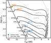 |
Fig. 1 Hertzsprung-Russell diagram of the stars in M17 with PMS evolutionary tracks from MIST (solid black lines; Dotter 2016; Choi et al. 2016; Paxton et al. 2011, 2013, 2015). The blue dots represent the PMS stars with IR excess and emission lines in their X-shooter spectrum. The orange triangles represent the PMS stars without emission lines in the X-shooter spectrum, but with IR excess λ > 2.3 µm (Chini et al. 2005). The gray striped line is the birth line, and the straight black line to the left of the figure is the ZAMS. The dotted gray lines show the isochrones. The ages are indicated in a similar color in the figure. |
2.2 Spectroscopy
For the six targets, optical to NIR observations (300–2500 nm) were obtained with the X-shooter spectrograph mounted on UT2 of the VLT (Vernet et al. 2011). This study is based on three to six epochs in the period 2009–2019. The spectra presented in RT17 comprise the first, and in some cases, the second epoch between 2009 and 2013. An additional two to three epochs were obtained in 2019 as part of a larger program in search for close binaries among the young OB stars in M17 (ESO program 0103.D-0099). We refer to Table 1 for a log of the observations and to Table A.1 for a detailed overview.
The X-shooter observations were performed under good weather conditions; the seeing ranging between 0.5″ and 1.2″ and a clear sky. The slit width used in the UVB arm (300– 590 nm) was 1″ (R 5100), except for the 2012 spectrum of B289 and the science verification spectrum of B275 in 2009, which were taken with a slit width of 0.8″ (R 6200) and 1.6″ (R 3300), respectively. For the VIS arm (550–1020 nm), a slit width of 0.9″ (R 8800) was used, except for the 2012 spectrum of B289, which had a slit width of 0.7″ (R 11 000). The NIR arm (1000– 1480 nm) observations were taken before 2019 with a slit width of 0.4″ (R 11 300) and in 2019 with a slit width of 0.6″ (R 8100). The exception for the NIR arm is the 2009 spectrum of B275, which had a slit width of 0.9″ (R 5600). All spectra were taken in nodding mode.
Overview of X-shooter epochs of the sample in M17.
2.2.1 Data reduction
The spectroscopic data were reduced with the ESO X-shooter pipeline 3.3.5 (Modigliani et al. 2010). This pipeline consists of a bias subtraction, a flat-field correction, and a wavelength calibration. The flux calibration was made with spectrophotometric standards from the ESO database. The initial reduction was made with the xsh_scired_slit_nod recipe provided in the software package from ESO. Furthermore, the Molecfit 1.5.9 tool was used to correct for the telluric sky lines (Smette et al. 2015; Kausch et al. 2015).
2.2.2 Nebular subtraction
All targets have residuals in the spectra that are caused by the subtraction of strong nebular emission in the nodding mode. As the nebular line emission varies along the slit both in strength and position, this reduction left stronger residuals for some targets that overlapped the emission features, which are broader than what can be expected from the width of a nebular emission line and the spectral resolution. To mitigate these problems, a more advanced nebular fitting routine developed by van Gelder et al. (2020; NebSub method) was applied to the four stars with severe nebular extinction that overlaps with line emission from the gaseous circumstellar disk. The contamination does not substantially affect the analysis of the remaining stars. In order to use this method, spectra obtained at different nodding positions were reduced individually in staring mode without sky subtraction. The two consecutive nodding observations of B268 on July 6 2012 are added in the staring mode, leading to a total of five instead of six observations for this object.
The NebSub method determines the strength of the forbidden nebular lines on-source and in the sky spectrum (off-source) by fitting these lines along the sky on the 2D slit because they are assumed to have a nebular contribution only. With the help of the nebular forbidden lines on-source and off-source, the scaling in strength and position is determined. This yields the nebular model spectrum that is subtracted from the source.
The nebular lines in B268, B275, and B337 were corrected with the use of models based on double Gaussian fits to the nebular lines off-source. For B243, a flat-top Gaussian function was sufficient to model the nebular contamination, where only the UVB arm of X-shooter was corrected (used for spectral classification). However, residuals remained in several lines with a strong nebular component. Because the nebular lines are very strong in He I lines, some He I with hints of circumstellar emission (e.g., the meta-stable He I line at 1083 nm), still had to be excluded from the study in this paper.
Updated spectral type and stellar parameters of our sample stars.
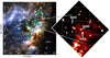 |
Fig. 2 Location of three PMS stars with gaseous disks in M17 (figure adapted from RT17). The zoomed-in region shows a VLT acquisition image taken with a 1.5′ × 1.5′ FoV technical CCD and a z′ filter. B243, B268 and B275 are in the same field of view and are indicated with the arrows. Nebular emission is present most prominently near B275 and B268. |
2.3 Photometry from acquisition images
The VLT acquisition images, taken with a 1.5′ × 1.5′ FoV technical CCD, provide photometric measurements in the z′ band of three stars in the sample that share their field of view. The z′ filter is part of the Sloan Digital Sky Survey filter system and covers the wavelength band 804–1350 nm. An example is shown in Fig. 2. The 17 observations of B243, B268, and B275 have the same time cadence as the spectroscopic data. The acquisition file of the science verification spectrum of B275 in 2009 is not available.
The acquisition images were analyzed using the aperture-photometry package Photutils (Bradley et al. 2020). The magnitudes are differential magnitudes with respect to the mean of three reference stars (circles in Fig. 3) that are close to the position of the three targets, such as to compare their magnitudes over the epochs and account for possible differences due to observing conditions.
Figure 3 shows the light curves, where the z′-band magnitudes are plotted as a function of Julian date. The differential z′ magnitudes are
 (1)
(1)
where  is the observed magnitude, and
  are the magnitudes of the reference stars i (circles in Fig. 3).
For B243 and B268, the ∆z′ magnitude varies by less than about 0.03 mag. Considering the potential variability of the reference stars (especially reference star 2), we therefore conclude that no significant photometric change is detected. Only B275 reveals significant variability; ∆z′ = 0.2 mag on timescales of hours in 2013 and ∆z′ = 0.1 mag in 2019 on a timescale of days. Unfortunately, the photometric observations with significant variability lack corresponding spectroscopic observations for B275.
3 Updating the spectral classification
Earlier classifications based on NIR spectroscopy by Hanson et al. (1997) and single-epoch X-shooter observations by RT17 can be improved by stacking the multiple spectra in this paper (we measured no radial velocity shifts between the epochs; see Sect. 7.2; nor did we measure significant variability in the lines we used for the classification). The higher signal-to-noise ratio together with the improved nebular subtraction allow the detection of weak features that enable a detailed spectral classification (Figs. 4 and 5).
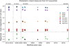 |
Fig. 3 z′-band magnitude measurements from 10 s exposures with the VLT acquisition camera. The sample includes three reference stars (circles), the mean of which was used to correct for observational differences between the acquisitions. The black-bordered stars represent acquisitions of stars in the sample with an accompanying X-shooter spectrum. |
3.1 B215
B215, previously classified as B0-B1V (RT17), shows a lack of He II lines and no C II at 426.7 nm in the stacked spectrum, implying a B1 spectral type. This is further confirmed by the He I lines 414.4 and 412.1 nm, which are about equally strong. Because there is no detection of O II at 435.0nm, the luminosity class V is confirmed (Liu et al. 2019), resulting in a B1 V classification.
3.2 B243
B243 was previously classified as B8 V (RT17) based on the He I lines (402.6, 400.9, and 447.1 nm). However, the nebula-corrected and stacked optical spectrum of all epochs reveal weaker He I lines than identified before. Because the Mg II 448.1 nm line is stronger than the He I 447.1 nm, this star is classified as a B9 star. The luminosity class is taken as III because He I 402.6 nm and Si II 412.8–413.0 nm are similar in strength (Liu et al. 2019), implying a B9 III.
3.3 B268
Earlier classifications of B268 led to B2V or B9-A0 (Hoffmeister et al. 2008, RT17). The stacked spectrum of B268 reveals relatively strong Mg II 448.1 nm lines compared to the neighboring
He I 447.1 nm, denoting a late-B or early-A type star. Additionally, because the He I 402.6 nm and 438.7 nm lines are weak, this points to a B9 star. Finally, the star is classified as B9 III, because He I 402.6 nm and Si II 412.8–413.0 nm are similar in strength (Liu et al. 2019).
3.4 B275
The B7 III classification of B275 by Ochsendorf et al. (2011) is confirmed based on a relatively strong Mg II feature at 448.1 nm compared to the He I at 447.1 nm with a ratio 3:2, indicating spectral type B7. The luminosity class is III due to the similar strength of the Si II lines at 412.8–3.0 nm and He I = 402.6 nm.
3.5 B289
This star shows He II absorption, but the He I 447.1 nm line is stronger than He II 454.0nm, so it must be an O8-O9 star. This is in line with the earlier classification of O9.7 V by RT17. The He II 420.0 nm absorption is visible in the stacked spectrum, it is weak, and thereby indicates O9-O9.7. Because He I 438.8 nm is stronger than He II 454.2 nm and He II 468.6 nm is stronger than C III 464.7/5.0/5.1 nm, the spectral type is O9.5. Si II 411.6 nm is weaker than He I 412.1 nm (Sota et al. 2011), so the classification becomes O9.5 V.
3.6 B337
The classification late-B by RT17 is adopted for the most deeply embedded star B337 based on SED fitting by Hanson et al. (1997). The stacking of the spectra did not improve the spectrum between 360 and 500 nm enough to allow for a detailed spectral classification.
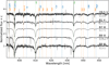 |
Fig. 4 Blue X-shooter spectrum of the PMS stars. The spectrum is stacked over all epochs and shows Balmer lines (green labels) and He I lines (orange labels). The remaining features are marked in blue. B337 is not detected in the blue due to the high extinction. The spectra of B215 and B289 were not nebula-subtracted. A sharp emission feature is present in addition to the hydrogen features. The ratio of the Mg II 448.1 nm (blue label) and He I 447.1 nm line changes with spectral type. A strong DIB is present at 443 nm (blue label). |
 |
Fig. 5 Part of the X-shooter stacked spectrum centered at the Ca II triplet. The spectra show broad photospheric profiles, and the PMS stars with gaseous disks include double-peaked emission features. The spikes are residuals from the nebular emission subtraction. Note the Ca II triplet (blue labels) and O I (blue label) emission in the Paschen series (green labels) lines. The Ca II triplet blends with Pa-13, Pa-15 and Pa-16. |
 |
Fig. 6 Diagram showing the four diagnostics used to infer (variability) properties of double-peaked emission lines. The peak-to-peak velocity corresponds to the velocity difference between the central velocities of the two peaks (orange). The heights of the peaks are divided to obtain the V/R ratio (green). The difference between the middle of the central peaks and the rest wavelength gives a central wavelength shift or radial velocity shift (purple). The equivalent width of this line is determined between −250 and −150 km s−1 and between 150 and 250 km s−1 (red). The (V/R)wing ratio is the ratio of these values. |
4 Methods
In this section, we discuss the methods we used to identify and characterize the lines originating from the circumstellar material to determine the spectral properties of the double-peaked emission lines and to measure the temporal variability of the circumstellar lines. The method section is structured in the same way as the subsequent sections, where we present the results (Sects. 5–7).
4.1 Circumstellar lines
RT17 identified emission lines that they linked to a circumstellar rotating disk. These lines are often double peaked and rest on top of a photospheric absorption line. We identified these and more circumstellar features by subtracting a stellar model from the spectrum. The stellar model was a BT-NextGen atmospheric model computed with the PHOENIX code (Hauschildt et al. 1999; Allard et al. 2012) with stellar parameters as determined by RT17 with FASTWIND modeling. The residual spectrum, referred to as the disk spectrum, shows the circumstellar material, which can have different components; a disk, a disk wind, an accretion flow, and/or a jet. They provide the opportunity of studying the structure, the dominant physical processes, and the material in the disk.
Additionally, the EW (and its errors) of the disk emission lines was calculated following Vollmann & Eversberg (2006) for low- and high-flux lines. We only determined the EW for a handful of emission lines in each star, because we only wished to measure uncontaminated lines. This is only possible for lines with little to no nebular subtraction residuals. Therefore, we excluded B337 from this procedure. The measured disk lines and the corresponding EWs are listed in Table D.2 for B243, B268, and B275.
4.2 Double-peaked line properties
The double-peaked emission lines are well pronounced, and the two peaks can be modeled with a double-Gaussian profile and a linear component, the latter to model the local continuum. Figure 6 shows a hypothetical disk-only spectral line that would result from a star model subtraction. We illustrate the four diagnostics we used to infer the characteristic line properties. Two of them are discussed in this section: (a) the peak-to-peak velocity, and (b) the V/R ratio. The other two diagnostics are discussed in Sects. 4.3.2 and 4.3.3 because they are evaluated over time.
The peak-to-peak velocity is measured as the distance between the center of the two peaks of the Gaussian model, illustrated by the orange arrows in Fig. 6. Half of this velocity yields an approximation for the projected rotational velocity of the disk region where the bulk of the line emission originates.
The heights of the blue (V) and red (R) peak of the Gaussian model were obtained after correcting the peak fluxes for the linear continuum, illustrated by the green arrows in Fig. 6. The ratio of these two peak values is the V/R ratio. The ratio is unity when the peak height is identical.
4.3 Spectroscopic variability
4.3.1 Temporal variance spectrum
Spectroscopic variability is identified in spectral lines using the temporal variance method (TVS, Fullerton et al. 1996; de Jong et al. 2001). This method compares the observed standard deviation of the flux σobs with the expected standard deviation of the flux σexp in a given wavelength bin. If the ratio of the two standard deviations is higher than unity, the variation in the spectral line between the epochs is stronger than what can be expected from the noise at that particular wavelength. When no variation is detected, the value of the TVS is randomly distributed around unity due to the noise in the data.
The σexp is calculated by averaging the standard deviation in the continuum regions around the spectral line in each epoch, yielding σcon, which is scaled by the square root of the ratio between the mean continuum flux and the mean (normalized) flux of the evaluated wavelength bin j for all epochs of observation. The σobs,j is directly calculated from observed fluxes in the wavelength bin. The ratio is given by
 (2)
(2)
where  the average continuum flux, and
  is the average flux in the wavelength bin j over all epochs. To determine the significance of the variability, the TVS value is compared to a χ2-distribution, where the degrees of freedom are given by the number of observations plus the number of lines with a similar TVS pattern. Only variability at a probability limit of 95% was considered.
In this study, we applied the TVS method to detect the line-of-sight velocity regimes that display significant variability. Assuming that the variability originates from the circumstellar disk and that the disks are in Keplerian rotation, we calculated where these velocities would originate in a rotating disk by assuming an inclination angle of the disk relative to the line of sight (based on earlier studies of these stars, Backs et al. 2023; Poorta et al. 2023). The TVS method does not produce realistic results in the central parts of lines that have a nebular contribution because residual nebular emission features between observing epochs cause a spurious variability signal. Inspection of the TVS signal generally provides a good way to distinguish between a spurious variability signal, which is often restricted to a few velocity bins, and intrinsic line variability is often observed over a wider velocity range or in multiple lines (Fullerton et al. 1996).
Anticipating the results of this study, we find that the TVS method indeed distinguishes between sources that display significant line variability and sources that do not. B243, B268, and B275 are in the first category, and B215, B289, and B337 do not show detectable variability (see Figs. C.1–C.3). In particular, the spectra of B337 are relatively noisy and nebular contamination is severe, which renders the TVS signal too weak to allow for any conclusions to be drawn. The TVS may show a marginal detection at most (in the blue peak of the Ca II triplet; see Fig. C.3).
 |
Fig. 7 Overview of O I, [O I], Fe I, Fe II, C I, and Br-γ lines in B243, B268, B275, and B337. The multiple epochs are overplotted, and the wavelengths are shown above each panel in nm. The [O I] and Fe II lines of B337 are not shown because the bluer part of the X-shooter spectrum is too noisy. All stars display some nebular emission (residuals) on the Br-γ emission (right panel). The variability between the epochs is discussed in Sect. 7. |
4.3.2 Radial velocity shift
The radial velocity of a system is measured as the difference between the central velocity of a photospheric absorption profile and the rest wavelength of the spectral line. However, the radial velocity can also be derived from double-peaked disk lines (if the disk is relatively symmetric and not circumbinary) by taking the difference between the middle of the blue and red peak and subtracting the rest wavelength value. This method was employed in this study. The striped purple arrow in Fig. 6 points to the middle velocity of the blue and red peak.
4.3.3 Variations in double-peaked line properties
We calculated the ratio of the EW in corresponding velocity intervals in the blue and red wings of the line, (V/R)wing ratio to avoid nebular contamination (not depicted in Fig. 6) and investigate the innermost parts of the disk. In Fig. 6, this is illustrated for the velocity intervals [±150, ±250] km s−1. Wherever this property is used in the analysis, the velocity interval is clearly indicated in the relevant figures. The wavelength ranges were chosen to enclose the largest interval without contamination in any of the lines. The chosen velocity regimes were the same for every line and epoch of a target.
The (V/R)wing ratios, peak-to-peak velocities, and V/R ratios were measured for each epoch in order to search for trends in their temporal variations.
5 Circumstellar lines
In this section, we describe the lines in the disk spectrum (after stacking and stellar model subtraction; see Sect. 4.1) of the four stars with gaseous disks (B243, B275, B268, and B337).
The stacked spectrum allows a detailed characterization of lines; no (inverse) PCygni profiles are identified, and the stars show (newly detected for B337) CO bandhead emission (Figs. 5–8). Other features in the disk spectrum are lines from H I, O I, and Ca II in all targets, and Na I, Mg I, C I, Fe I/Fe II, and [O I] in some.
A detailed discussion of the presence, strength, and shape of the spectral lines is provided in Appendix B. A characterization of the lines in the circumstellar spectra of the stars is given in the next section, supported by Table 3. The table consists of emission and absorption lines that are detected in the spectrum. For the latter, this means that they are not present in the star model and could not be tied to a stellar origin (see Sect. 8.3 for a discussion of this). Despite the nebular subtraction described in Sect. 2, nebular line residuals remain present in some of the lines, especially in H I. Consequently, the central several dozen km s−1 of these lines cannot be used.
All stars show H I emission. The strongest double-peaked Balmer, Paschen, and Bracket emission is present in B243, and they are weakest in B337 (Fig. 5).
O I lines are observed in all stars in absorption and emission. However, only B243, B275, and B337 have double-peaked emission at 844.6 nm and 1128.7 nm. The emission is strongest in B243, which alone shows the O I triplet at 777.4 nm in emission.
The Ca II triplet is weakest in B243. It is even weaker than the overlapping double-peaked Paschen features. In the other objects, these lines are stronger than the Paschen features. In particular, the peaks in B275 and B337 are stronger and closer together than the lines in B268. A similar trend is seen for Mg I double-peaked emission at 880.7 nm. This line is strongest for B275, weaker for B268, weakest in B337, and absent in B243.
Comparable behavior is seen in Fe II at 999.8 nm: It is strongest in B275 and absent in B243. Other Fe I and Fe II lines appear in the spectra as weak absorption or double-peaked emission in B268 and B275. The S/N of the stacked disk spectrum of B337 is too low for a detection of the weak Fe lines.
Multiple double-peaked C I emission is present in the spectra of B243 and B275, the two stars for which 0 I 844.6 nm emission is observed and that have the strongest hydrogen lines. The carbon lines are detected at wavelengths >900 nm. In B275, these lines are mostly stronger than the Fe double-peaked emission lines. One C I line is also present in B337, which shows a small O I 844.6 nm emission line.
B268 is the only star with Na I (589.0 nm and 589.6 nm) absorption. These absorption lines reside alongside narrow absorption lines originating from the interstellar medium.
Last, the CO bandheads are strongest in B268 and B275, and they are much weaker in B243 and B337 (Fig. 8). This is the first detection of CO bandhead emission in B337. The strength of this feature also depends on the continuum emission (Poorta et al. 2023).
 |
Fig. 8 Stacked NIR X-shooter spectra of the PMS stars. All sources except for B215 and B289 display CO bandhead emission (vertical dotted green lines), indicating the presence of a hot circumstellar disk. We detect CO in B337 for the first time. The dashed blue lines show the Pſund series. The narrow absorption features correspond to residuals from the telluric correction. |
Circumstellar spectrum overview in B243, B268, B275, and B337.
6 Double-peaked line properties
In this section, we discuss the results from the line diagnostics described in Sect. 4.2. B337 is not shown in this section because of a lack of double-peaked emission lines.
6.1 Peak-to-peak velocities
The peak-to-peak separation ranges between 135–180 km s−1 for B243, 220–300 km s−1 in B268, and 80–160 km s−1 for B275. Half of the peak-to-peak velocities, the so-called disk velocities, for one epoch per star are shown on the x-axis of Fig. 9.
In Fig. 9, B243 shows a trend in which the projected disk velocity is higher for higher-order hydrogen lines (indicated by the more transparent colors). This can be understood in terms of disk rotation and the lower-excitation lines (indicated by the darker colors) which are formed over a larger extent of the disk up to where the velocities are lower, with a correspondingly larger radiation area. This trend is observed in the hydrogen (green and blue), oxygen (purple) and carbon lines (red). This behavior is similarly observed in the hydrogen lines of B275 (green), while other lines are more scattered. High projected disk velocities are measured for the Ca II triplet, Mg I, and C I lines. The velocities of the O I lines in B243 and B275 are lower by some dozen km s−1, more similar to the lower excitation hydrogen lines.
6.2 V/R ratio
Figure 9 shows the V/R ratio in all stars for double-peaked lines. Remarkably, in B243 and B275 the values vary from lower to higher than unity for transitions in a single epoch, meaning that the highest peak is sometimes the red and sometimes the blue peak. A common interpretation is that the V/R ratio traces an asymmetry of the circumstellar disk. The observations suggest a higher degree of complexity (azimuthal variations, e.g., a spiral arm; see Sect. 8.1.2). B243 and the H I lines in B275 both show a trend that the lines with the lowest V/R ratio have the lowest peak velocity.
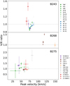 |
Fig. 9 The peak velocity (half the peak-to-peak velocity) of all double-peaked emission lines in B243, B268, and B275 is plotted against their V/R ratios. The data points represent the line properties in one epoch of each star. The emission lines in a single epoch of a star have different V/R ratios and peak velocities. For B243 and B275, the lower excitation lines form at relatively lower velocities, hence at more slowly rotating parts of the disk, and their V/R ratios are relatively lower, meaning that their red peak is stronger than the blue, than measured for the higher excitation lines. For both stars, this results in a trend of a higher V/R ratio with a higher disk velocity. The displayed epochs are for B243: 2012-07-06, B268: 2019-05-31, and B275: 2019-07-09. |
7 Spectroscopic variability
In this section, we discuss the results from characterizing the variability with the TVS method, potential radial velocity changes, and temporal variance in the line diagnostics. The methods in Sect. 4.3 were used to quantify the variability of the PMS stars.
7.1 Temporal variance spectrum
The cadence of our observations allows us to probe variations on timescales of days, months, and years. In principle, the individual nodding positions that are taken at intervals of 10–20 min might be used to also probe characteristic timescales of about an hour. On these timescales, however, no intrinsic variability is seen.
We find that the TVS method reveals significant variations in the H I, O I, Ca II, and Na I lines of B243, B268, and B275 up to velocities of ~360, ~320, and ~370 km s−1 , respectively, in both the red and blue wings of the lines. These velocities are significantly higher than the observed v sini (see Sect. 8.1.3). Hα shows the strongest variations on the shortest (about days) timescales. Lower-order hydrogen lines show more pronounced variability than their higher-order counterparts.
Generally, the velocity interval in which variability is observed is consistent in the line series, for instance, in the Paschen or Bracket series. The velocity interval and amplitude of the variability differ for different atomic species in a single source (e.g., in B243, the O I lines vary at lower velocities on the blue side than in the H I lines). Moreover, the variability detected in one atomic species may differ in the different stars (e.g., the Paschen series in B243 shows variability on the red and blue side, but the Paschen series in B275 mostly shows variability on the red side). However, for all stars, the O I lines show stronger variability at the red side than at the blue side of the lines.
To help visualize the location in the disk at which the variability originates, the 1D TVS profile was mapped to a 2D Keplerian disk model (see Sect. 4.3.1). The colors in the disk maps display the average TVS profile as measured for a series of lines in a certain object, and they are shown in the middle panels of Figs. 10–12. The height of the color bar was determined for each average TVS profile based on the highest TVS measure outside of the nebular line interval, which is not shown in the map. This leaves a blue color in the regions with a zero velocity with respect to the observer. Each velocity bin of the TVS profile is projected in a face-on view of the disk, adopting an average inclination of 70° for the sources. Inclinations of 60° or 80° do not substantially affect the projected maps. The left side of the disk map shows the blueshifted velocities, and the right side of the disk map shows the redshifted velocities.
In the following parts, we discuss the (significant) variability detected in the three PMS stars with a gaseous disk.
B243
B243 displays significant variability in the hydrogen Banner, Paschen, and Bracket series, as well as in the O I lines. We detect variability on the blue and red sides of the lines at velocities up to ~360 km s−1 in Hα and up to ~350 km s−1 for the Paschen and Bracket series (Fig. 10). The O I lines show strong variability on the red side at velocities up to ~300 km s−1, and variability up to much lower velocities of ~180 km s−1 on the blue side. The detected variations are similar for the O I lines and the H I lines, as shown in their (average) TVS profiles. However, these average H I and O I TVS profiles differ as seen on the disk maps, while the profiles of the Paschen and Bracket series are very similar to each other. The central two disk maps in Fig. 10 for the Paschen and Bracket series show a similar profile: variability on both sides of the disk that is slightly stronger on the red than on the blue side. The leftmost and rightmost maps also show strong red-side variability, but while hardly any variability is detected at the blue side of the O I lines, very strong variability is detected on the blue side of the Banner lines.
Because the Ca II triplet emission is weaker than the imposed Paschen emission, this feature was excluded from the analysis. We detect variability in all lines for the shortest probed timescale, which is four days.
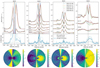 |
Fig. 10 TVS and disk maps for B243. The emission lines in B243 that display variability are shown in the upper panel (first row). The middle panel displays the TVS for each emission line (light blue) and an average profile (dark blue) calculated for each series of lines is displayed in the upper panel. The variations at the line center of the H I lines are residuals from the nebular subtraction. The TVS panel shows the continuum level as a dotted line at unity, and a gray line marking the level at which variations reach the 95% significance level. The average TVSs in the lower panels in each column are mapped onto the circles in the bottom row. They show a face-on disk view, where the TVS is mapped according to their velocity bins. The gray circles and accompanying numbers are in units of the stellar radius. The white areas are the result of the disk projection and do not have any physical meaning. |
B268
Variability in B268 is observed in the strongest hydrogen lines (up to Paδ), the Ca II triplet, O I at 777 nm triplet, and the Na I doublet. The Hα and the Pa series are characterized by a strong blue peak and variability on both sides of the feature up to 320 km s−1 for the former and up to 220 km s−1 for the latter (Fig. 11). The red-peak variations of the Ca II lines are not reliable because of residuals from the subtraction of the overlapping nebular Paschen emission lines. All three calcium lines show similar variations in the blue peak up to 160 km s−1. This variability is similar to the variability in the blue peak of the Paschen series, where the first two observations in 2019 show the weakest features of all epochs. Furthermore, variations in the Na I doublet are characterized by additional absorption that is superimposed on the red side of the interstellar Na I contribution, which is only detected in the observations of 2012 and 2013. Variations in the O I triplet are detected on the red side and are visible in all epochs.
B275
Variations in B275 are most pronounced on the red side of all emission lines, with the exception of the Ca II lines. Variability is detected at velocities up to ~370 km s−1 for the Balmer and Paschen series (Fig. 12) and up to ~320 km s−1 for the O I lines. All species vary between the 2009 observation and those in 2019. Additionally, monthly and daily variability is detected in the lower-order hydrogen lines and in the O I lines.
In the double-peaked emission of O I 844.6 nm (at ± 120 km s−1), the blue peak has a higher amplitude than the red peak, but the variability in the red peak is stronger, as shown in the TVS profile (Fig. 12). In contrast, the Ca II triplet shows a stronger red peak, and the 2009 spectrum displays stronger lines overall.
7.2 Radial velocity shifts
Earlier studies of massive young stars in M17 reported a lack of short-period binaries, revealed by the low radial velocity dispersion (σ1D) observed in single-epoch observations of a sample of 12 stars (Sana et al. 2017). Our multi-epoch approach provides the opportunity of searching for radial velocity variations (which are indicative of close binarity) in our sample stars.
No radial velocity changes of >20 km s−1 are detected based on measurements of the disk lines from one epoch to the next for all of the stars. This limit is often used for the detection of short-period binaries (Sana et al. 2013). Furthermore, the shifts in the double peaks correspond to the shifts in the radial velocity of the measured interstellar absorption lines that we measured for reference. These shifts are therefore attributed to differences in wavelength calibration between the epochs. This is supported by the estimated radial velocity shift of the interstellar absorption lines. This demonstrates the potential of using the center of the double peaks to measure radial velocity shifts.
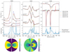 |
Fig. 11 TVS and disk maps for B268; see the caption of Fig. 10. Although the blue emission peaks are stronger, variability seems to be relatively equal on both sides. |
7.3 Peak-to-peak velocity variations
Similar to what is observed for a single epoch (Fig. 9), the peak-to-peak velocities differ among the double-peaked lines, and their respective temporal differences are generally similar.
Only small (<20 km s−1) peak-to-peak velocity variations are detected on timescales of days, months, and years for all PMS stars (Fig. E.2). The three epochs in 2019 for B243 show a marginal temporal trend in their respective variations of ~5 km s−1 for most lines. Similarly, a marginal temporal trend is seen in B268 for all epochs, but the small number of available double-peaked emission lines makes this detection less significant. The peak-to-peak velocity variations in B275 are relatively small (<l0 km s−1) for all but two Fe I/Fe II lines, which show a similar marginal temporal trend.
7.4 (V/R)wing ratio variations
For B243, the variability detected in the (V/R)wing ratio follows a similar trend for all lines, with the exception of Hα and Hβ (Fig. E.3). However, in the last epoch, a decrease in the V/Rwing ratio is observed for all lines. For the Paschen and Bracket series, the ratio reaches as high as 2.2 in the first three epochs and exceeds 3 for O I, and it subsequently decreases toward or below
1. This indicates that the red side is stronger than the blue side. The (V/R)wing ratio for Hα is below unity for all epochs.
A detailed of study of the wings of Paschen and Bracket lines in Fig. 10 shows the origin of this temporal trend of the (V/R)wing ratio, especially for the observations in 2019. All Paschen and Bracket wings in the first observation of 2019 (green line, 201907-30) show wing excess emission on the blue side compared to the other epochs. Four days later, in the second observation of 2019 (red line, 2019-08-03), this excess in the wing on the blue side has diminished in all Paschen and Bracket lines. A few weeks later, during the last observation in 2019 (purple line, 2019-09-25), we observe a wing excess on the red side of the all Paschen and Bracket lines compared to the other epochs.
We compare this with V/R ratio variations in B243, which show a similar trend for most lines (Fig. E.1). The ratio of the Paschen, Bracket, and O I lines varies between ~0.85 to ~1.3 in a single epoch, which is less than seen for the (V/R)wing ratio. During most of the epochs, most lines have a ratio >1, indicating a stronger blue than red peak flux.
In B268, the width of the nebular lines is similar to the peak-to-peak separation in the hydrogen lines. We therefore did not use the V/R ratio, but focused on the (V/R)wing ratio. The high-velocity (V/R)wing ratio for B268 is >1 for all lines at all epochs, showing that the blue wing is consistently stronger than the red wing. In the case of B275, we do not detect strong temporal variations in the V/R ratio. However, a strong decrease in the (V/R)wing ratio is observed on the longest observed timescale (2009–2019). This is due to a drop in flux on the red side of the features. No significant variations in the (V/R)wing ratio are observed on timescales of months and days. The exception to this is Hβ, which shows a decrease in the ratio on a daily timescale and an increase a few weeks later.
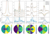 |
Fig. 12 TVS and disk maps for B275; see the caption of Fig. 10. In all lines, the red side shows more variability close to the star than the blue side. |
8 Discussion
We present an overview of the characteristics of spectroscopic and photometric variability in our sample of PMS stars and discuss scenarios that might cause this variability. We explore the scenario of a spiral arm in the disk of B243 and B275 based on the systematic differences in spectral lines in a single epoch. The sample is compared with spectroscopic variability in intermediate-mass YSOs to place the PMS stars in M17 in a pre-main-sequence evolutionary context. The properties of the variability in our sample are used as a diagnostic tool to identify a candidate MYSO in M17.
8.1 Spectroscopic variability and its possible origins
The spectroscopic variability in this study comprises differences between the spectra of the studied PMS stars (Fig. 5 and Table 3), temporal variations between all epochs in three of the four PMS stars with gaseous disks (Figs. 10–12 and C.4), and differences in the temporal variation of (series of) spectral lines in a single PMS star and among the stars (Figs. 10–12). The spectral differences and variability indicate that different physical processes are simultaneously at work in the gaseous circumstellar disks, and they suggests that (at least a subset of) these processes may act locally and/or have a time-dependent nature.
Variations are strongest in double-peaked emission lines and are observed in the peaks and in the wings of these lines. Assuming that the emission originates in a Keplerian rotating disk, the spatial origin of the peaks is related to the location where the bulk of the emission is produced and that of the wings to the innermost part of disk. In general, hot gas emitting in the optical and NIR traces the inner regions of PMS stars. The spectral lines of T Tauri and Herbig Ae/Be stars in these wavelength domains can display many variable processes due to accretion (bursts), jets, disks structures (that could be the remains of the disk formation process), disk dispersal and/or disk winds, and possibly stellar multiplicity (e.g., Mora et al. 2004; Mendigutía et al. 2011; Ellerbroek et al. 2014; Schöller et al. 2016; Contreras Peña et al. 2017; Moura et al. 2020; Stock et al. 2022; Zsidi et al. 2022).
Although a stellar origin of the variability (e.g., starspots, pulsations, or flares) cannot be excluded, the high velocities at which the variations occur and the asymmetries in them point to a circumstellar origin. Therefore, we refrain from further discussion of stellar scenarios and instead focus on possible origins associated with a circumstellar disk.
The mechanisms that we exclude as a possible cause of the observed variability are strong accretion bursts, jets, and close binaries (of similar masses). The first due to the lack of strong photometric variations (we observe a variation of 0.2 mag at most; see Sect. 8.2) and (inverse) PCygni profiles typical for such bursts. Jets are unlikely because we do not detect high-velocity components associated with forbidden emission lines, and for close binarity, we lack evidence of radial velocity variations (> 20 km s−1) and/or periodically varying light curves.
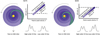 |
Fig. 13 Sketch of the disk for an epoch in B275 and B243. The positive trend of the V/R ratio and the peak-to-peak velocity might be explained by a spiral arm in the disks of B275 and B243. We show two examples of face-on inner gaseous disks with a spiral arm and line-forming regions in the disk of the higher- and lower-order HI lines, where the line region of the latter extends to the surface of the star. Typical double-peaked emission lines are shown for these HI lines. The panels that show the V/R ratio on the y-axis and the peak-to-peak velocity on the x-axis mimic the epochs shown in Fig. 9. |
8.1.1 Typical timescales of the spectral variability
The shortest measured variability timescale is a few days. This is observed in all stars with spectral variability, in the hydrogen Balmer, Paschen, and Bracket series and in O I lines. The daily variability is often stronger than variations between two epochs that are weeks or years apart, although a pronounced variation on a timescale of years is revealed in some targets (e.g., in the Paschen lines of B243 and B275, and the Na I doublet in B268). Therefore, the processes causing the line variability must include mechanisms that manifest on timescales of days and that may be transient in nature with a recurrence time up to some years at most.
8.1.2 Relation of the peak-to-peak velocity to the V/R ratio
The Paschen and Bracket lines in B243 and the Paschen lines in B275 show a positive trend in the peak-to-peak velocity to the V/R ratio, as displayed in Fig. 9 in a single epoch. For B275, this ratio changes in a single epoch from an about equal red and blue peak (V/R ~ 1) in the lower series lines (which form over a relatively large region of the disk; see e.g. Backs et al. 2023, and they therefore have lower peak-to-peak velocities) to a stronger blue peak in the higher order H I lines (which form in the inner regions of the disk, hence have relatively strong peak-to-peak velocities). This behavior cannot be reconciled in the context of an axisymmetrically rotating disk and could imply additional structure in the disk that crosses the line of sight at this particular epoch.
One option that could explain this trend is a spiral arm in the disk, where a high-density optically thin or hotter optically thick structure resides in the inner parts of the disk (moving toward the observer, hence the stronger blue peak in the high-excitation lines) that wavers out to larger distances (explaining the more or less equal red and blue peak strength in the low-excitation lines), see Fig. 13. For B243, a similar scenario may hold, but the density enhancement of the spiral arm there starts on the other side in the inner disk because the V/R ratio changes from below unity to about unity and higher in a single epoch. For this star, additional indications exist in 2019 in particular for a rotating high-density structure at high velocities (see Fig. E.3). Nevertheless, the complexity of the line of sight toward a PMS star (e.g., winds, as discussed in Sect. 8.5) complicates the identification of such a structure in all epochs. We do not attempt this in this work.
We conclude that for both B275 and B243, there is evidence for disk inhomogeneities perhaps similar to variations in the V/R4 ratio that trace the high-density part of a one-arm oscillation in Be-star disks (Telting & Kaper 1994). The fact that we detect the V/R ratio changes in one epoch more clearly than in the others could be an effect of the rotation of the structure with respect to the line of sight. Simulations of (massive) star formation show that substructures are common in the inner-disk regions of massive YSOs and PMS stars, and that they could persist throughout PMS evolution (e.g., Meyer et al. 2017; Kölligan & Kuiper 2018; Oliva & Kuiper 2020). We remark, however, that not all line variability characteristics can be explained in this way, which leaves room for other phenomena that may be at work simultaneously.
8.1.3 Variability at high velocity
To help determine the location of the spectroscopic variations in different lines might originate in the disk, we measured the maximum velocity at which significant variability is detected in each hydrogen line of the Balmer and Paschen series. This was done both on the blue and red side, and we plot this against the oscillator strength times the wavelength (“line strength”) in Fig. 14. In B243 and B268, the maximum velocity increases with increasing oscillator strength. This also is the case for the blue side of the Balmer lines in B275, but not for the red side, for which this maximum velocity is fairly constant at about 300km s−1. It might be hypothesized that the rising trends are due to an obser vational bias: for stronger lines, it is easier to detect variability up to higher velocities. However, the trend is absent on the red side in B275.
In Hα, variability is detected up to 320 km s−1 at least, signi fying that the inner disk must rotate with such high velocities.
In order to test whether this can be consistent with the lines forming in a Keplerian rotating disk, the velocity expected at a given radius for different inclination angles is shown in Fig. 15. The stellar mass and projected surface rotation velocity v sini are taken from Table 2. In this case, the maximum velocities can be explained with an inclination >55° for B243 and B268 if the disk reaches the surface of the star. For B275, only an inclination of >80° can explain the highest measured emission line velocities. This is not consistent with the inclination measurement of B275 from Poorta et al. (2023; ~60°) based on modeling of CO bandhead emission.
Alternatively, the high velocities may be explained by invoking corotation (of the inner disk), leading to the high-velocity emission originating from gas at about 3.5 R★ in the case of B243, 4 R★ for B275, and from ~8 R★ for B268. Corotation may be enforced if the disk gas is strongly coupled to a stellar surface magnetic field, as is probably the case in the innermost disk regions of T Tauri and Herbig Ae stars, where magnetospheric accretion may be at play. It is unclear whether magnetic fields play a dominant role in the accretion process of the more massive Herbig Be stars (Mendigutía 2020; Vioque et al. 2022). In this respect, it is noteworthy and surprising that an alternative to a Keplerian velocity profile seems to best fit the most luminous (hence, most massive) source B275. We conclude that for B243 and B268, the high-velocity emission may be explained by a disk that extends almost to the surface.
As the red-side variability is observed up to high velocities in B275 regardless of the studied H I line, and because the maximum Hα velocity can only be explained in a Keplerian rotating disk seen edge on, the cause of the variability might be connected to an origin different than this rotating disk. The variability at these high velocities might be caused by an accretion flow that crosses the line of sight. A magnetically forced corotating inner disk up to at least 3.5 R★ cannot be excluded as an explanation of the Ha velocity. However, this scenario seems less likely because a visual inspection of the spectral lines in Fig. 12 shows that the spectrum in 2009 displays redshifted absorption compared to the observations in 2019.
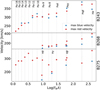 |
Fig. 14 Maximum velocity at which significant variation is observed in the TVS (over all epochs) for each star, plotted against the oscillator strength times the wavelength. The maximum velocities are determined on the red and blue side of the features. We plot the absolute blue-side velocity for convenience. The blue velocities of the Paschen lines of B275 are not shown because they do not display variability at high velocities, which makes them indistinguishable from nebular subtraction residuals (which range from ~50–80 km s−1). |
8.2 Photometric variability
B243 and B268 do not reveal significant photometric variability (Δ z’′ ≲ 0.03 mag; see Fig. 3). For B275, variations Δ z′ ~ 0.1 − 0.2 mag are seen on timescales of hours to days at two of the four observing moments in which multiple observations have been secured. T Tauri stars, the lower-mass counterpart of our sources, generally show recurring outbursts and photometric variability, often connected to episodes of (increased) mass-accretion rates (e.g., Contreras Peña et al. 2017; Cody et al. 2017; Zsidi et al. 2022), where the amplitude of the photometric variations correlates with the characteristic timescales of the events (Fischer et al. 2023). The strongest outbursts are seen in FU Orionis stars (4–6 mag on timescales of years to decades) and EX Lupi stars (2–4 mag on timescales of about a year). As we probe similar timescales of years to a decade, these types of outburst are likely excluded for our sources. For T Tauri stars, 0.5–2 mag outbursts have been observed during magnetospheric accretion events. This type of irregular and smaller accretion events might cause the small shifts in Δ z′ in B275 because it has been shown that the amplitude of the photometric variations may depend on the band that is probed (Ellerbroek et al. 2014) as well as on the inclination of the system (Kesseli et al. 2016). However, it may also be related to other phenomena that operate on timescales of hours or days, such as stellar flares, pulsations, small companions, starspots if the star is magnetic, or other phenomena that operate on dynamical or rotational timescales of the star or the innermost part of the disk (Fischer et al. 2023).
8.3 Potential origin of the emission lines
Although the behavior of the line variability is complex, certain lines show variations that appear to be correlated in time as well as in strength. Specifically, these are the O I line at 844.6 nm and 1128.7 nm, C I and H I emission in B243, B275, and (weakly) in B337, and the Ca II triplet, Mg I, and Fe I at 999.8 nm emission in B268, B275, and B337 (see Table 3). Likely, these correlations could imply that the same mechanism causes the variations.
The simultaneous presence of strong O I and H I lines is due to Bowen resonance fluorescence, where Lyβ photons excite the O I resonance line 2p  at 102.58 nm, from which they cascade through the O I at 844.6 nm and the 1128.7 nm lines follow. This has been identified as the dominant excitation mechanism of O I lines in Herbig Be stars (Mathew et al. 2018) and is a well-known phenomenon in H II regions. The link implies that O I emission is cospatial with (optically thick) H I Lyman excitation, where Ha was used by Mathew et al. (2018) as a tracer for Lyman excitation.
For B243 and B275, the velocity regimes in which variability is detected for Hα and O I agree (Figs. 10 and 12), which further underlines this connection. Both stars also show double-peaked C I emission. To our knowledge, C I emission has not been associated with any pumping by hydrogen or helium resonance lines, similar to O I. We note that the stars with the strongest O I emission also show a handful of double-peaked C I emission lines. This may imply a relation that is yet to be investigated with the (destruction of) CO molecules, which are observed as CO-bandhead emission in both stars. In literature, C I observations are only discussed in the context of T Tauri stars, where they were used as a parameter to characterize the formation of planets (McClure 2019).
We do not observe variations in the CO-bandhead emission, which consists of superpositions of many CO transitions. The superpositions complicate the detection of variability. However, relatively strong changes in the disk, in inclination, in midplane disk density or midplane disk temperature where the CO band-heads are thought to form (Ilee et al. 2018; Poorta et al. 2023) should be observable, as was shown in an extreme case during an accretion outburst, for example (Caratti o Garatti et al. 2017).
A strong Ca II triplet and Mg I and Fe I at 999.8 nm emission are simultaneously present in B268, B275, and B337, but none of the lines appears (strongly) in B243. The variability in the Ca II triplet emission is characterized by variability in the peaks in B268 and B275. The other lines do not vary.
The variability in the Ca II triplet and O I lines are not correlated, which is similar to what is observed in Be stars (Shokry et al. 2018). These authors concluded that the origin of the variability in the two species should be attributed to processes that are spatially separated, possibly caused by independent mechanisms acting in the disk.
B268 is the only star with superimposed Na I (D1 and D2) absorption lines on the sharp Na I absorption lines that arise from the ISM. Variability is detected in these lines between 2012/2013 and 2019, where the absorption has disappeared. Variability in the Na I lines is also observed in intermediate-mass YSOs (Mora et al. 2004; Mendigutía et al. 2011), where the variations are linked to the circumstellar disk.
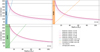 |
Fig. 15 Projected radial velocity profiles for various models. The left filled-in region in each panel denotes the stellar size. Two velocity-distance relations are plotted: 1. Corotation with the stellar surface, where the velocity increases away from the star, and 2. Keplerian rotation for several inclinations, where the velocity increases towards the star. The striped lines present the maximum Hα velocity detected in the disk (in black), determined by the extent of the variability, and the Ha velocity determined by the average of half of the peak-to-peak velocity (in gray). |
8.4 Considerations regarding mass-accretion rate estimates
As part of the final stage of formation, PMS stars undergo accretion. The rate of accretion  may help determine the evolutionary phase of the system, and when infall of material from the natal cloud has ceased, the remaining lifetime of the disk. The mass-accretion rates of T Tauri and Herbig stars are estimated from ultraviolet (UV) or Balmer-continuum excess, which is thought to be due to gas, funneled along magnetic field lines that connect the inner disk to the star, which shocks the photosphere upon impact. The exact relation between
  and the additional luminosity caused by accretion Lacc depends on several factors, including the impact velocity, the fraction of surface that is filled by accretion columns, the quiet-surface stellar temperature, and the inner-disk radius (e.g., Fairlamb et al. 2015). This additional luminosity caused by accretion is empirically found to correlate with the emission line luminosity (e.g., Mendigutía et al. 2011; Fairlamb et al. 2017). This does not suggest that all the line emission originates from the accretion stream; it may originate from both the infalling gas and gas that is in Keplerian orbit in the inner disk. For instance, Peña et al. (2017) and Backs et al. (2023) showed that hydrogen emis sion lines can be reproduced by adopting a stationary Keplerian disk model alone. The scatter in Lacc − Lline relations typically amounts to an order of magnitude (e.g., Fairlamb et al. 2017; Vioque et al. 2022). This implies that care should be taken when interpreting the resulting mass-accretion rates, especially when no direct indications of mass accretion are observed.
No UV or Balmer continuum photometry is not available for our sources. We therefore resorted to using line luminosities to obtain the mass-accretion rates. We used the lines with an equivalent width measurement in Table D.2 and SEDs from RT17 to obtain the absolute line luminosities, and we applied the relations provided in Fairlamb et al. (2017). The resulting accretion rates for each epoch are presented in Fig. 16 and Table D.1. We obtain typical values of ~10−6−10−5 M⊙ yr−1, comparable to what is found for Herbig Be stars (Mendigutía et al. 2011, 2013; Fairlamb et al. 2015; Ababakr et al. 2017; Wichittanakom et al. 2020; Vioque et al. 2022; Brittain et al. 2023).
When we adopt a typical time for our sources to arrive on the ZAMS of ~105 yr (see Fig. 1), the disk should have a mass of ~0.1 M⊙ to remain present for the full span of this remaining PMS evolution. Recent estimates of the masses of the disks of B243, B268, and B275 from ALMA continuum observations only yield masses of about 10−3 M⊙ (Poorta et al., in prep.), implying that these disks will be cleared in ~100−1000 yr for these derived mass-accretion rates. It seems unlikely that we detected these stars at such a critical time. This further emphasizes that the derived  must be handled with care.
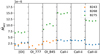 |
Fig. 16 Accretion rates from spectral line luminosities in M⊙ yr−1 for B243, B268, and B275. Each bracketed column is for a given line and shows the rates for all epochs separately. The values should be considered with care given the uncertainties associated with the applied method (see text), but they are typically ~10−6 M⊙ yr−1 for B243 and B268, and up to ~10−5 M⊙ yr−1 for B275. |
8.5 Slow disk winds and jets
In T Tauri stars, the shape and strength of (blueshifted) observed forbidden lines (Natta et al. 2014), notably [O I] at 630 nm, probably indicate the escape of gas from the PMS system, either in a slow wind emanating from the disk surface (Nisini et al. 2018), or in high-velocity jets that are emitted in the polar directions. B243 and B275, and tentatively B268, have [O I] at 630 nm in emission (see Fig. 7). The velocities at which the line is in emission range from about [−50, 50] km s−1. When the peak is observed at these velocities, which are close to the system velocity, as is the case here, it is for T Tauri stars that are classified as a low-velocity component (Edwards et al. 1987; Nisini et al. 2018). Systems that show emission lines with a high-velocity component (HVS; >200 km s−1) likely feature jets that arise from the mass-accretion process (Ellerbroek et al. 2014).
An origin of [O I] at 630 nm in a flow that is launched away from the disk surface is supported by the single-peaked nature of the line (while allowed lines coming from the disk are typically double-peaked). For a disk inclination of 70°, a jet with velocities up to 146 km s−1 beaming in the direction normal to the disk surface would also show a projected velocity of 50 km s−1. However, jets are usually associated with early stages of PMS evolution and seem at odds with the apparently low disk masses inferred by Poorta et al. (in prep.). These jets often give rise to multiple forbidden-line transitions, such as [F II], [Ni II], and [S II] (Ellerbroek et al. 2014), which are not observed in the PMS stars. A slow disk wind in B243, B268, and B275 seems a more plausible outflow model assuming that T Tauri stars and more massive PMS stars have similar disk wind and jet mechanisms.
8.6 Variability as a means to identifying circumstellar material
Three of the four stars with gaseous disks of the six PMS stars show spectroscopic variations in their optical and NIR emissio lines at relatively high velocities (> 100 km s−1). There is no observed variability in the spectra of B215 and B289 (Figs. C.1-C.2), which do not show emission lines (outside of the range affected by nebular lines >50 km s−1). B337 has emission lines, but also shows strong nebular subtraction residuals and is heavily extincted, which restricts the detection of variability in this star (Fig. C.4). This result shows that variability from the hot disk gas could be a common property in PMS stars with gaseous disks in M17, and it also shows that strong nebular emission in M17 complicates the detection of emission for stars with emission lines with velocities ~50–100 km s−1 (e.g., which originate from a fairly face-on disk). Assuming that this type of spec-troscopic variability is a more common property in PMS stars, we could use this as a diagnostic to identify stars with gaseous circumstellar material.
To test this potential diagnostic, we applied it to identify circumstellar material around the other stars from the spectro-scopic monitoring campaign of OB stars in M17 (see Sect. 2.1). Based on the TVS method, one of the stars, B205, shows significant spectroscopic variations in multiple lines up to 200 km s−1 (Fig. 17). This star was classified by Povich et al. (2017) as a B2 star by its NIR colors and J-band magnitude. Although Hanson et al. (1997) did not detect infrared excess for this source, Backs et al. (in prep.) placed this star on the PMS track in the HRD. This star might still feature a remnant gaseous disk, which would challenge our understanding of disk removal, or this star might have developed into a Be star, despite the young age of M17 (~0.65±0.25 Myr; Stoop et al. 2024). More investigation is needed to confirm or reject a pre-main-sequence nature for B205.
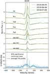 |
Fig. 17 Line profiles and TVS of B205. The upper panel shows the Balmer, Paschen, Bracket, and helium lines in several spectra of B205 taken in 2019. The lower panel shows the TVS of these spectra, indicating a significant velocity range between −150 km s−1 and 220 km s−1. The variations in the spectra appear to be strongest in the helium lines. The emission around the rest wavelength of the features is of nebular origin, as confirmed by their 2D spectra. |
9 Conclusion
This paper presented a multi-epoch study of simultaneous spectroscopic and photometric observations of six PMS stars in M17; four with gaseous disks and two PMS stars with IR excess redward of 3.0 μm. These PMS stars with observable photospheres and gaseous disks exhibit intrinsic variability (except for the most deeply embedded star).
Spectroscopic variability is observed on all timescales (especially in strong emission lines), which range from days to years, and the variablitly seems to be transient over the longer timescales of months and years. The extent and timescale of the variability differs per line and object, which shows the complexity of the physical conditions in the regions in which the different lines are formed. This leads us to posit that multiple processes are at play, causing variations in these gaseous disks.
In one epoch of B243 and B275, we observe a positive trend of the V/R ratio with projected rotational velocity as measured from different double-peaked emission lines. In both cases, the V/R ratio takes values above and below unity, which in this particular case might indicate a structure in the disk that crosses the line of sight, such as a spiral arm. Other differences in the spec tral line set show that two similar PMS stars (B243 and B268) with the same central object in terms of spectral type, age, and mass show differences in disk properties.
The weak peak-to-peak velocity variations between the epochs and the consistency in the double-peak morphology for lines in each epoch show that the bulk of the probed disk region is relatively stable or that temporal effects are adequately smeared out. This is supported by the fact that we do not observe variations in the CO bandhead emission. Variability is largely confined to the disk region close to the surface of the star and to disk structures on top of or in the relatively stable bulk of the disk.
Determining the maximum velocity of the variations shows that variability is detected at high velocities (>320 km s−1), indi cating an origin close to the surface of the stars. For B275, the highly variable velocities on the red side of the H I lines, independent of the H I line strength, indicate an origin of the variability in an accretion flow from the inner-disk region to the star. However, the lack of strong photometric variations (in all stars) shows that this flow cannot cover a significant fraction of the star or disk, and strong accretion bursts (of EX Lupi or FU Orionis type) are excluded.
The presence of a low-velocity component in [O I] at 630 nm that does not vary shows that we have to take relatively slow outflows or winds into account that could be launched from the disk.
Our PMS stars do not seem to fit the empirically determined  relation. When we assume that these objects are still accreting, the estimated mass accretion rates show much higher accretion rates than expected for these PMS stars. This might be due to a different accretion mechanism for the more massive Herbig stars, accompanied by a different
  relation that is currently not accounted for in mass-accretion estimates for the more massive PMS stars.
The spectroscopic variability shows that multiple processes are at play in these PMS stars with gaseous disks. The next step is to obtain more multi-epoch spectroscopy of a larger sample of stars to tie variability to a certain phase in the pre-main-sequence evolution and to more specifically link variations to certain disk processes.
Acknowledgements
We thank the anonymous referee for carefully reading the manuscript and many helpful and insightful comments and suggestions. We acknowledge support from the Netherlands Research School for Astronomy (NOVA). This research has made use of the SIMBAD database, operated at CDS, Strasbourg, France (Wenger et al. 2000). This research made use of Astropy, a community-developed core Python package for Astronomy (Astropy Collaboration 2022). This work has made use of data from the European Space Agency (ESA) mission Gaia (https://www.cosmos.esa.int/gaia), processed by the Gaia Data Processing and Analysis Consortium (DPAC, https://www.cosmos.esa.int/web/gaia/dpac/consortium). Funding for the DPAC has been provided by national institutions, in particular the institutions participating in the Gaia Multilateral Agreement.
Appendix A Observations
The observations for each star and date are listed in the table below and show exposure times for each observation in a particular arm.
Exposure times and S/N for each observation.
Appendix B Circumstellar lines
We provide a detailed discussion of emission and absorption lines in the spectrum for each of the four PMS stars with a gaseous disk.
Appendix B.1 B243
The spectrum of B243 is characterized by (double-) peaked line emission in H I, Ca II, and O I. The Paschen and Bracket absorption lines are superimposed with two clearly separated emission peaks. Only the strongest Balmer lines are partly visible in emission.
In particular, while photospheric wings are detectable as blue as Ba-13/Ηθ, emission is not observed in Hγ and the bluer H I lines. A narrow residual from the nebular subtraction is still present in all H I lines. For the Paschen series, this is visible as a small peak of ~50 km s−1 in width around the rest wavelength, while for the Balmer series, the contamination is broader, with a width of ~160 km s−1 at the bottom of the feature. This relatively broad range compared to the intrinsic width of nebular lines is caused by variations in the nebular emission lines along the slit, which increase the affected region during the subtraction of these lines (see Sec. 2.2.2).
The double-peaked Ca II triplet is weaker than the Paschen lines. The features blend. Therefore, only a weak blue peak of the Call appears in the wings of the Paschen lines. O I emission is observed at 844.6 nm, double-peaked in emission, and likewise for the triplet at 777.4 nm, but weaker. Additionally, the O I triplet is present in absorption at 926.2-926.6 nm. Last, the forbidden [O I] at 630.0 nm appears single-peaked in all of the spectra in emission. The C I lines appear double-peaked in emission for wavelengths longer than 900 nm. B243 shows weaker CO bandhead emission than B268 and B275.
Appendix B.2 B268
The inner core of the H I lines is strongly affected by the residuals of the nebular subtraction. Therefore, the analysis of B268 focuses on lines lacking nebular components and the broader, lower-order H I lines, which show emission. Because the width of the nebular emission is wider than the width between potential double peaks, we cannot distinguish the shape of the profile.
All H I lines show photospheric absorption. For Hβ, Hα, Paδ, Paγ, Paβ, and Brγ, this absorption is partially filled in by emission. For all of these lines, the blue side of the emission feature is stronger than the red side. The O I line at 844.6 nm is contaminated by nebular emission, and the O I triplet lines at 777.4 nm and at 926.2-926.6 nm are in absorption. [O I] 630.0 nm is single-peaked and in emission.
The Ca II emission superimposed on the Paschen lines is strongly in emission. Only the blue peak of the feature can be used for analysis due to the blend. In contrast to B243, the CaII triplet lines are broader and stronger than the blended Paschen lines. The Fe lines are weak and in absorption, except for Fe II 999.8 nm, which is single-peaked and in emission. There is double-peaked Mg I emission at 880.8 nm, and the Na I doublet (D1 and D2) shows an absorption component on the red side in addition to the interstellar one. B268 shows the first and second overtone of the CO bandhead in emission. The bandhead profiles are characterized by a strong blue shoulder.
Appendix B.3 B275
Photospheric absorption lines are observed in all H I lines in the available wavelength range. Emission starts to fill in this absorption from Hδ to longer wavelengths and is clearly visible in both wings from Hβ. Similar to the stars discussed previously, the region around the rest wavelength of several lines is affected by residuals left from the subtraction of nebular emission. This region extends from 100-170 km s−1 (see B243 and Sec. 2.2.2 for comments on the width) for the Balmer series to 50-80 km s−1 for the Paschen series. While for some Paschen lines, the double peaks are detected, for most lines, it is impossible to distinguish between a double and a single peak. For all these H I lines, the blue wing seems stronger than the red wing.
The stronger blue peak is also visible in the double-peaked O I at 844.6 nm. The O I triplets at 777.3 nm and 926.2-926.6 nm appear in absorption, and there is single-peaked [O I] emission at 630.0 nm. The Ca II triplet appears double-peaked in emission and is stronger than the Paschen lines. While the blue feature shows two equally strong peaks, the redder features have stronger red peaks. Many C I and Fe lines show as double-peaked emission that varies in strength. Only Fe II 999.8 nm exhibits a single peak. The Mg I line at 880.8 nm is observed in emission with a double-peaked profile. B275 shows first- and second-overtone CO bandhead emission. The profile shows a tiny blue shoulder.
Appendix B.4 B337
Because B337 is the most deeply embedded target, the spectrum is obscured for wavelengths shorter than 840 nm, with the exception of the Ha emission. For Hα, Paδ, Paγ, Paβ, and Brγ the emission is broader than the nebular emission, allowing for a disk detection but no further analysis.
The spectra show a double-peaked Ca II triplet, double-peaked O I emission at 844 nm, and Mg I emission at 880.8 nm, where the latter two lines only become apparent in the stacked spectrum. Fe II at 999.8 nm is in emission. This peak is broad, and because of the amount of noise in the spectrum, it is not pos sible to distinguish whether this is two peaks or one broad peak. The O I triplets at 777.3 nm and 926.2-926.6 nm are in absorption and the CO bandhead emission is weak, where the clearest detection is the second peak of the first overtone (at 2322.76 nm).
Lines detected in the spectra (star + circumstellar) of B243, B268, B275, and B337.
Appendix C TVS of B215, B289 and B337
Appendix D Equivalent width and mass-accretion rates
In this section, we present the EWs of a handful of lines and the mass-accretion rates that follow from the methods described in Sec. 4.1 for the EW and in Sec 8.4 for the mas-accretion rates. In order to measure the EW O I at 844.6 nm, which is blended with Pa-18, the average EW of Pa-17 and Pa-19 was subtracted from the EW of the blended O i and Pa-18. The Ca II triplet isblended with the Pa-16, Pa-15, and Pa-13 lines, and the EW should therefore be taken as an upper limit.
Mass-accretion rates in M⊙ year−1
EW measurements of lines without nebular contamination in B243, B268, and B275 in A. In case of the Ca II, the EWs are an upper limit
Appendix E Peak-to-peak, V/R ratio, and (V/R)wing ratio
This section shows the peak-to-peak velocities and (V/R)wing ratio for each star in each epoch. Relative changes over time are discussed in Sec. 7.3 and 7.4. The V/R ratio for each epoch in B243 is shown for comparison with changes in the (V/R)wing ratio, which is highest for this star.
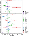 |
Fig. E.1 V/R ratio of the peaks of the double-peaked emission features in B243. Most lines follow a similar trend in ratio over the several epochs. Part of the lines are < 1 in the first three epochs, indicating a stronger red than blue peak. This changes for the last two epochs, where most of the lines have a stronger blue than red peak. |
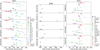 |
Fig. E.2 Peak-to-peak velocity of the double-peaked emission lines in the spectra of B243, B268, and B275 is shown on the x-axis, and the date of observation is plotted on the y-axis. The peaks are measured after subtracting the stellar feature by a double-Gaussian fit. The velocities in B243 (left figure) range between 130 km s−1 and 180 km s−1, and there is a general trend in velocity over the five epochs, which is most apparent for all lines in the last three epochs. In B268 (middle panel), the velocities range between 220km s−1 and 300 km s−1, and the velocity difference is 65 km s−1 between the Ca II triplet and Mg I peak-to-peak velocities (the legend of B275 can also be used to read the middle panel). The velocities in B275 (right panel) range from 70 km s−1 to 165 km s−1. |
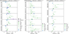 |
Fig. E.3 (V/R)wing ratio measurements of the double-peaked emission features after subtracting a star model shown on the x-axis. The observation date is plotted on the y-axis. In the left panel for B243, the EW is determined between ±100 km s−1 and ±300 km s−1; in the middle panel for B268, it is between ±90 km s−1 and ±290 km s−1, and in the right panel for B275, it is between ±90 km s−1 and ±240 km s−1. |
References
- Ababakr, K. M., Oudmaijer, R. D., & Vink, J. S. 2017, MNRAS, 472, 854 [NASA ADS] [CrossRef] [Google Scholar]
- Allard, F., Homeier, D., & Freytag, B. 2012, Philos. Trans. Roy. Soc. Lond. Ser. A, 370, 2765 [NASA ADS] [Google Scholar]
- Astropy Collaboration (Price-Whelan, A. M., et al.) 2022, ApJ, 935, 167 [NASA ADS] [CrossRef] [Google Scholar]
- Audard, M., Ábrahám, P., Dunham, M. M., et al. 2014, in Protostars and Planets VI, eds. H. Beuther, R. S. Klessen, C. P. Dullemond, & T. Henning, 387 [Google Scholar]
- Backs, F., Poorta, J., Rab, C., et al. 2023, A&A, 671, A13 [NASA ADS] [CrossRef] [EDP Sciences] [Google Scholar]
- Baines, D., Oudmaijer, R. D., Porter, J. M., & Pozzo, M. 2006, MNRAS, 367, 737 [NASA ADS] [CrossRef] [Google Scholar]
- Bik, A., Kaper, L., & Waters, L. B. F. M. 2006, A&A, 455, 561 [CrossRef] [EDP Sciences] [Google Scholar]
- Bradley, L., Sipocz, B., Robitaille, T., et al. 2020, https://doi.org/18.5281/zenodo.4844744 [Google Scholar]
- Brittain, S. D., Kamp, I., Meeus, G., Oudmaijer, R. D., & Waters, L. B. F. M. 2023, Space Sci. Rev., 219, 7 [NASA ADS] [CrossRef] [Google Scholar]
- Cabrit, S., Edwards, S., Strom, S. E., & Strom, K. M. 1990, ApJ, 354, 687 [Google Scholar]
- Caratti o Garatti, A., Stecklum, B., Garcia Lopez, R., et al. 2017, Nat. Phys., 13, 276 [Google Scholar]
- Carpenter, J. M., Hillenbrand, L. A., & Skrutskie, M. F. 2001, AJ, 121, 3160 [NASA ADS] [CrossRef] [Google Scholar]
- Castelli, F., & Kurucz, R. L. 2003, in Modelling of Stellar Atmospheres, 210, eds. N. Piskunov, W. W. Weiss, & D. F. Gray, A20 [NASA ADS] [Google Scholar]
- Chini, R., Hoffmeister, V. H., Nielbock, M., et al. 2005, in Massive Star Birth: A Crossroads ofAstrophysics, 227, eds. R. Cesaroni, M. Felli, E. Churchwell, & M. Walmsley, 145 [NASA ADS] [Google Scholar]
- Choi, J., Dotter, A., Conroy, C., et al. 2016, ApJ, 823, 102 [Google Scholar]
- Cody, A. M., Hillenbrand, L. A., David, T. J., et al. 2017, ApJ, 836, 41 [Google Scholar]
- Contreras Pefla, C., Lucas, P. W., Kurtev, R., et al. 2017, MNRAS, 465, 3039 [NASA ADS] [CrossRef] [Google Scholar]
- de Jong, J. A., Henrichs, H. F., Kaper, L., et al. 2001, A&A, 368, 601 [NASA ADS] [CrossRef] [EDP Sciences] [Google Scholar]
- Dotter, A. 2016, ApJS, 222, 8 [Google Scholar]
- Edwards, S., Cabrit, S., Strom, S. E., et al. 1987, ApJ, 321, 473 [Google Scholar]
- Ellerbroek, L. E., Kaper, L., Bik, A., et al. 2011, ApJ, 732, L9 [NASA ADS] [CrossRef] [Google Scholar]
- Ellerbroek, L. E., Podio, L., Dougados, C., et al. 2014, A&A, 563, A87 [NASA ADS] [CrossRef] [EDP Sciences] [Google Scholar]
- Fairlamb, J. R., Oudmaijer, R. D., Mendigutia, I., Ilee, J. D., & van den Ancker, M. E. 2015, MNRAS, 453, 976 [NASA ADS] [CrossRef] [Google Scholar]
- Fairlamb, J. R., Oudmaijer, R. D., Mendigutia, I., Ilee, J. D., & van den Ancker, M. E. 2017, MNRAS, 464, 4721 [NASA ADS] [CrossRef] [Google Scholar]
- Fischer, W. J., Hillenbrand, L. A., Herczeg, G. J., et al. 2023, in ASP Conf. Ser., 534, Protostars and Planets VII, 355 [NASA ADS] [Google Scholar]
- Fitzpatrick, E. L. 1999, PASP, 111, 63 [Google Scholar]
- Frost, A. J., Oudmaijer, R. D., de Wit, W. J., & Lumsden, S. L. 2021, A&A, 648, A62 [NASA ADS] [CrossRef] [EDP Sciences] [Google Scholar]
- Fullerton, A. W., Gies, D. R., & Bolton, C. T. 1996, ApJS, 103, 475 [NASA ADS] [CrossRef] [Google Scholar]
- Gaia Collaboration 2022, VizieR Online Data Catalog: I/355 [Google Scholar]
- Hanson, M. M., Howarth, I. D., & Conti, P. S. 1997, ApJ, 489, 698 [NASA ADS] [CrossRef] [Google Scholar]
- Hauschildt, P. H., Allard, F., Ferguson, J., Baron, E., & Alexander, D. R. 1999, ApJ, 525, 871 [Google Scholar]
- Hoffmeister, V. H., Chini, R., Scheyda, C. M., et al. 2008, ApJ, 686, 310 [NASA ADS] [CrossRef] [Google Scholar]
- Hollenbach, D., Johnstone, D., Lizano, S., & Shu, F. 1994, ApJ, 428, 654 [NASA ADS] [CrossRef] [Google Scholar]
- Hollenbach, D. J., Yorke, H. W., & Johnstone, D. 2000, in Protostars and Planets IV, eds. V. Mannings, A. P. Boss, & S. S. Russell, 401 [Google Scholar]
- Hosokawa, T., Omukai, K., Yoshida, N., & Yorke, H. W. 2011, Science, 334, 1250 [CrossRef] [Google Scholar]
- Ilee, J. D., Fairlamb, J., Oudmaijer, R. D., et al. 2014, MNRAS, 445, 3723 [Google Scholar]
- Ilee, J. D., Oudmaijer, R. D., Wheelwright, H. E., & Pomohaci, R. 2018, MNRAS, 477, 3360 [CrossRef] [Google Scholar]
- Kausch, W., Noll, S., Smette, A., et al. 2015, A&A, 576, A78 [NASA ADS] [CrossRef] [EDP Sciences] [Google Scholar]
- Kesseli, A. Y., Petkova, M. A., Wood, K., et al. 2016, ApJ, 828, 42 [NASA ADS] [CrossRef] [Google Scholar]
- Kölligan, A., & Kuiper, R. 2018, A&A, 620, A182 [NASA ADS] [CrossRef] [EDP Sciences] [Google Scholar]
- Kuiper, R., & Hosokawa, T. 2018, A&A, 616, A101 [NASA ADS] [CrossRef] [EDP Sciences] [Google Scholar]
- Kumar, M. S. N., Contreras Peña, C., Lucas, P. W., & Thompson, M. A. 2016, ApJ, 833, 24 [NASA ADS] [CrossRef] [Google Scholar]
- Liu, Z., Cui, W., Liu, C., et al. 2019, ApJS, 241, 32 [CrossRef] [Google Scholar]
- Mathew, B., Manoj, P., Narang, M., et al. 2018, ApJ, 857, 30 [NASA ADS] [CrossRef] [Google Scholar]
- McClure, M. K. 2019, A&A, 632, A32 [NASA ADS] [CrossRef] [EDP Sciences] [Google Scholar]
- Mendigutía, I. 2020, Galaxies, 8, 39 [Google Scholar]
- Mendigutía, I., Eiroa, C., Montesinos, B., et al. 2011, A&A, 529, A34 [EDP Sciences] [Google Scholar]
- Mendigutía, I., Brittain, S. D., Eiroa, C., et al. 2013, ApJ, 776, 44 [CrossRef] [Google Scholar]
- Meyer, D. M. A., Vorobyov, E. I., Kuiper, R., & Kley, W. 2017, MNRAS, 464, L90 [Google Scholar]
- Modigliani, A., Goldoni, P., Royer, F., et al. 2010, SPIE Conf. Ser., 7737, 773728 [Google Scholar]
- Mora, A., Eiroa, C., Natta, A., et al. 2004, A&A, 419, 225 [NASA ADS] [CrossRef] [EDP Sciences] [Google Scholar]
- Morales-Calderón, M., Stauffer, J. R., Hillenbrand, L. A., et al. 2011, ApJ, 733, 50 [CrossRef] [Google Scholar]
- Moura, T., Alencar, S. H. P., Sousa, A. P., Alecian, E., & Lebreton, Y. 2020, MNRAS, 494, 3512 [NASA ADS] [CrossRef] [Google Scholar]
- Muzerolle, J., D'Alessio, P., Calvet, N., & Hartmann, L. 2004, ApJ, 617, 406 [CrossRef] [Google Scholar]
- Natta, A., Testi, L., Alcalá, J. M., et al. 2014, A&A, 569, A5 [NASA ADS] [CrossRef] [EDP Sciences] [Google Scholar]
- Nisini, B., Antoniucci, S., Alcalá, J. M., et al. 2018, A&A, 609, A87 [EDP Sciences] [Google Scholar]
- Ochsendorf, B. B., Ellerbroek, L. E., Chini, R., et al. 2011, A&A, 536, A1 [NASA ADS] [CrossRef] [EDP Sciences] [Google Scholar]
- Oliva, G. A., & Kuiper, R. 2020, A&A, 644, A41 [NASA ADS] [CrossRef] [EDP Sciences] [Google Scholar]
- Peña, P., Sigut, T. A. A., & Landstreet, J. D. 2017, ApJ, 836, 214 [CrossRef] [Google Scholar]
- Paxton, B., Bildsten, L., Dotter, A., et al. 2011, ApJS, 192, 3 [Google Scholar]
- Paxton, B., Cantiello, M., Arras, P., et al. 2013, ApJS, 208, 4 [Google Scholar]
- Paxton, B., Marchant, P., Schwab, J., et al. 2015, ApJS, 220, 15 [Google Scholar]
- Pecaut, M. J., & Mamajek, E. E. 2013, ApJS, 208, 9 [Google Scholar]
- Pogodin, M. A., Pavlovskii, S. E., Beskrovnaya, N. G., et al. 2022, Astrophysics, 65, 31 [NASA ADS] [CrossRef] [Google Scholar]
- Poorta, J., Ramírez-Tannus, M. C., de Koter, A., et al. 2023, A&A, 676, A122 [NASA ADS] [CrossRef] [EDP Sciences] [Google Scholar]
- Povich, M. S., Busk, H. A., Feigelson, E. D., Townsley, L. K., & Kuhn, M. A. 2017, ApJ, 838, 61 [NASA ADS] [CrossRef] [Google Scholar]
- Puls, J., Urbaneja, M. A., Venero, R., et al. 2005, A&A, 435, 669 [NASA ADS] [CrossRef] [EDP Sciences] [Google Scholar]
- Ramírez-Tannus, M. C., Kaper, L., De Koter, A., et al. 2017, A&A, 604, A78 [NASA ADS] [CrossRef] [EDP Sciences] [Google Scholar]
- Ramírez-Tannus, M. C., Cox, N. L. J., Kaper, L., & de Koter, A. 2018, A&A, 620, A52 [NASA ADS] [CrossRef] [EDP Sciences] [Google Scholar]
- Rivero González, J. G., Puls, J., Najarro, F., & Brott, I. 2012, A&A, 537, A79 [NASA ADS] [CrossRef] [EDP Sciences] [Google Scholar]
- Sana, H., de Koter, A., de Mink, S. E., et al. 2013, A&A, 550, A107 [NASA ADS] [CrossRef] [EDP Sciences] [Google Scholar]
- Sana, H., Ramírez-Tannus, M. C., de Koter, A., et al. 2017, A&A, 599, A9 [Google Scholar]
- Schöller, M., Pogodin, M. A., Cahuasquí, J. A., et al. 2016, A&A, 592, A50 [NASA ADS] [CrossRef] [EDP Sciences] [Google Scholar]
- Shokry, A., Rivinius, T., Mehner, A., et al. 2018, A&A, 609, A108 [NASA ADS] [CrossRef] [EDP Sciences] [Google Scholar]
- Smette, A., Sana, H., Noll, S., et al. 2015, A&A, 576, A77 [NASA ADS] [CrossRef] [EDP Sciences] [Google Scholar]
- Sota, A., Maíz Apellániz, J., Walborn, N. R., et al. 2011, ApJS, 193, 24 [Google Scholar]
- Stock, C., McGinnis, P., Caratti o Garatti, A., Natta, A., & Ray, T. P. 2022, A&A, 668, A94 [NASA ADS] [CrossRef] [EDP Sciences] [Google Scholar]
- Stoop, M., Derkink, A., Kaper, L., et al. 2024, A&A, 681, A21 [NASA ADS] [CrossRef] [EDP Sciences] [Google Scholar]
- Telting, J. H., & Kaper, L. 1994, A&A, 284, 515 [NASA ADS] [Google Scholar]
- Uchiyama, M., & Ichikawa, K. 2019, ApJ, 883, 6 [NASA ADS] [CrossRef] [Google Scholar]
- van Gelder, M. L., Kaper, L., Japelj, J., et al. 2020, A&A, 636, A54 [NASA ADS] [CrossRef] [EDP Sciences] [Google Scholar]
- Vernet, J., Dekker, H., D'Odorico, S., et al. 2011, A&A, 536, A105 [NASA ADS] [CrossRef] [EDP Sciences] [Google Scholar]
- Vioque, M., Oudmaijer, R. D., Wichittanakom, C., et al. 2022, ApJ, 930, 39 [NASA ADS] [CrossRef] [Google Scholar]
- Vollmann, K., & Eversberg, T. 2006, Astron. Nachr., 327, 789 [Google Scholar]
- Wenger, M., Ochsenbein, F., Egret, D., et al. 2000, A&AS, 143, 9 [NASA ADS] [CrossRef] [EDP Sciences] [Google Scholar]
- Wichittanakom, C., Oudmaijer, R. D., Fairlamb, J. R., et al. 2020, MNRAS, 493, 234 [Google Scholar]
- Xu, Y., Moscadelli, L., Reid, M. J., et al. 2011, ApJ, 733, 25 [NASA ADS] [CrossRef] [Google Scholar]
- Zsidi, G., Fiorellino, E., Kóspál, Á., et al. 2022, ApJ, 941, 177 [CrossRef] [Google Scholar]
All Tables
Lines detected in the spectra (star + circumstellar) of B243, B268, B275, and B337.
EW measurements of lines without nebular contamination in B243, B268, and B275 in A. In case of the Ca II, the EWs are an upper limit
All Figures
|
Fig. 1 Hertzsprung-Russell diagram of the stars in M17 with PMS evolutionary tracks from MIST (solid black lines; Dotter 2016; Choi et al. 2016; Paxton et al. 2011, 2013, 2015). The blue dots represent the PMS stars with IR excess and emission lines in their X-shooter spectrum. The orange triangles represent the PMS stars without emission lines in the X-shooter spectrum, but with IR excess λ > 2.3 µm (Chini et al. 2005). The gray striped line is the birth line, and the straight black line to the left of the figure is the ZAMS. The dotted gray lines show the isochrones. The ages are indicated in a similar color in the figure. |
| In the text | |
|
Fig. 2 Location of three PMS stars with gaseous disks in M17 (figure adapted from RT17). The zoomed-in region shows a VLT acquisition image taken with a 1.5′ × 1.5′ FoV technical CCD and a z′ filter. B243, B268 and B275 are in the same field of view and are indicated with the arrows. Nebular emission is present most prominently near B275 and B268. |
| In the text | |
|
Fig. 3 z′-band magnitude measurements from 10 s exposures with the VLT acquisition camera. The sample includes three reference stars (circles), the mean of which was used to correct for observational differences between the acquisitions. The black-bordered stars represent acquisitions of stars in the sample with an accompanying X-shooter spectrum. |
| In the text | |
|
Fig. 4 Blue X-shooter spectrum of the PMS stars. The spectrum is stacked over all epochs and shows Balmer lines (green labels) and He I lines (orange labels). The remaining features are marked in blue. B337 is not detected in the blue due to the high extinction. The spectra of B215 and B289 were not nebula-subtracted. A sharp emission feature is present in addition to the hydrogen features. The ratio of the Mg II 448.1 nm (blue label) and He I 447.1 nm line changes with spectral type. A strong DIB is present at 443 nm (blue label). |
| In the text | |
|
Fig. 5 Part of the X-shooter stacked spectrum centered at the Ca II triplet. The spectra show broad photospheric profiles, and the PMS stars with gaseous disks include double-peaked emission features. The spikes are residuals from the nebular emission subtraction. Note the Ca II triplet (blue labels) and O I (blue label) emission in the Paschen series (green labels) lines. The Ca II triplet blends with Pa-13, Pa-15 and Pa-16. |
| In the text | |
|
Fig. 6 Diagram showing the four diagnostics used to infer (variability) properties of double-peaked emission lines. The peak-to-peak velocity corresponds to the velocity difference between the central velocities of the two peaks (orange). The heights of the peaks are divided to obtain the V/R ratio (green). The difference between the middle of the central peaks and the rest wavelength gives a central wavelength shift or radial velocity shift (purple). The equivalent width of this line is determined between −250 and −150 km s−1 and between 150 and 250 km s−1 (red). The (V/R)wing ratio is the ratio of these values. |
| In the text | |
|
Fig. 7 Overview of O I, [O I], Fe I, Fe II, C I, and Br-γ lines in B243, B268, B275, and B337. The multiple epochs are overplotted, and the wavelengths are shown above each panel in nm. The [O I] and Fe II lines of B337 are not shown because the bluer part of the X-shooter spectrum is too noisy. All stars display some nebular emission (residuals) on the Br-γ emission (right panel). The variability between the epochs is discussed in Sect. 7. |
| In the text | |
|
Fig. 8 Stacked NIR X-shooter spectra of the PMS stars. All sources except for B215 and B289 display CO bandhead emission (vertical dotted green lines), indicating the presence of a hot circumstellar disk. We detect CO in B337 for the first time. The dashed blue lines show the Pſund series. The narrow absorption features correspond to residuals from the telluric correction. |
| In the text | |
|
Fig. 9 The peak velocity (half the peak-to-peak velocity) of all double-peaked emission lines in B243, B268, and B275 is plotted against their V/R ratios. The data points represent the line properties in one epoch of each star. The emission lines in a single epoch of a star have different V/R ratios and peak velocities. For B243 and B275, the lower excitation lines form at relatively lower velocities, hence at more slowly rotating parts of the disk, and their V/R ratios are relatively lower, meaning that their red peak is stronger than the blue, than measured for the higher excitation lines. For both stars, this results in a trend of a higher V/R ratio with a higher disk velocity. The displayed epochs are for B243: 2012-07-06, B268: 2019-05-31, and B275: 2019-07-09. |
| In the text | |
|
Fig. 10 TVS and disk maps for B243. The emission lines in B243 that display variability are shown in the upper panel (first row). The middle panel displays the TVS for each emission line (light blue) and an average profile (dark blue) calculated for each series of lines is displayed in the upper panel. The variations at the line center of the H I lines are residuals from the nebular subtraction. The TVS panel shows the continuum level as a dotted line at unity, and a gray line marking the level at which variations reach the 95% significance level. The average TVSs in the lower panels in each column are mapped onto the circles in the bottom row. They show a face-on disk view, where the TVS is mapped according to their velocity bins. The gray circles and accompanying numbers are in units of the stellar radius. The white areas are the result of the disk projection and do not have any physical meaning. |
| In the text | |
|
Fig. 11 TVS and disk maps for B268; see the caption of Fig. 10. Although the blue emission peaks are stronger, variability seems to be relatively equal on both sides. |
| In the text | |
|
Fig. 12 TVS and disk maps for B275; see the caption of Fig. 10. In all lines, the red side shows more variability close to the star than the blue side. |
| In the text | |
|
Fig. 13 Sketch of the disk for an epoch in B275 and B243. The positive trend of the V/R ratio and the peak-to-peak velocity might be explained by a spiral arm in the disks of B275 and B243. We show two examples of face-on inner gaseous disks with a spiral arm and line-forming regions in the disk of the higher- and lower-order HI lines, where the line region of the latter extends to the surface of the star. Typical double-peaked emission lines are shown for these HI lines. The panels that show the V/R ratio on the y-axis and the peak-to-peak velocity on the x-axis mimic the epochs shown in Fig. 9. |
| In the text | |
|
Fig. 14 Maximum velocity at which significant variation is observed in the TVS (over all epochs) for each star, plotted against the oscillator strength times the wavelength. The maximum velocities are determined on the red and blue side of the features. We plot the absolute blue-side velocity for convenience. The blue velocities of the Paschen lines of B275 are not shown because they do not display variability at high velocities, which makes them indistinguishable from nebular subtraction residuals (which range from ~50–80 km s−1). |
| In the text | |
|
Fig. 15 Projected radial velocity profiles for various models. The left filled-in region in each panel denotes the stellar size. Two velocity-distance relations are plotted: 1. Corotation with the stellar surface, where the velocity increases away from the star, and 2. Keplerian rotation for several inclinations, where the velocity increases towards the star. The striped lines present the maximum Hα velocity detected in the disk (in black), determined by the extent of the variability, and the Ha velocity determined by the average of half of the peak-to-peak velocity (in gray). |
| In the text | |
|
Fig. 16 Accretion rates from spectral line luminosities in M⊙ yr−1 for B243, B268, and B275. Each bracketed column is for a given line and shows the rates for all epochs separately. The values should be considered with care given the uncertainties associated with the applied method (see text), but they are typically ~10−6 M⊙ yr−1 for B243 and B268, and up to ~10−5 M⊙ yr−1 for B275. |
| In the text | |
|
Fig. 17 Line profiles and TVS of B205. The upper panel shows the Balmer, Paschen, Bracket, and helium lines in several spectra of B205 taken in 2019. The lower panel shows the TVS of these spectra, indicating a significant velocity range between −150 km s−1 and 220 km s−1. The variations in the spectra appear to be strongest in the helium lines. The emission around the rest wavelength of the features is of nebular origin, as confirmed by their 2D spectra. |
| In the text | |
 |
Fig. C.1 Line profiles and TVS of B215. See the caption of Fig. 10. |
| In the text | |
 |
Fig. C.2 Line profiles and TVS of B289. See the caption of Fig. 10. |
| In the text | |
 |
Fig. C.3 Line profiles and TVS of the Ca II lines in B337. See the caption of Fig. 10. |
| In the text | |
 |
Fig. C.4 Line profiles and TVS of Ha in B337. See the caption of Fig. 10. |
| In the text | |
|
Fig. E.1 V/R ratio of the peaks of the double-peaked emission features in B243. Most lines follow a similar trend in ratio over the several epochs. Part of the lines are < 1 in the first three epochs, indicating a stronger red than blue peak. This changes for the last two epochs, where most of the lines have a stronger blue than red peak. |
| In the text | |
|
Fig. E.2 Peak-to-peak velocity of the double-peaked emission lines in the spectra of B243, B268, and B275 is shown on the x-axis, and the date of observation is plotted on the y-axis. The peaks are measured after subtracting the stellar feature by a double-Gaussian fit. The velocities in B243 (left figure) range between 130 km s−1 and 180 km s−1, and there is a general trend in velocity over the five epochs, which is most apparent for all lines in the last three epochs. In B268 (middle panel), the velocities range between 220km s−1 and 300 km s−1, and the velocity difference is 65 km s−1 between the Ca II triplet and Mg I peak-to-peak velocities (the legend of B275 can also be used to read the middle panel). The velocities in B275 (right panel) range from 70 km s−1 to 165 km s−1. |
| In the text | |
|
Fig. E.3 (V/R)wing ratio measurements of the double-peaked emission features after subtracting a star model shown on the x-axis. The observation date is plotted on the y-axis. In the left panel for B243, the EW is determined between ±100 km s−1 and ±300 km s−1; in the middle panel for B268, it is between ±90 km s−1 and ±290 km s−1, and in the right panel for B275, it is between ±90 km s−1 and ±240 km s−1. |
| In the text | |
Current usage metrics show cumulative count of Article Views (full-text article views including HTML views, PDF and ePub downloads, according to the available data) and Abstracts Views on Vision4Press platform.
Data correspond to usage on the plateform after 2015. The current usage metrics is available 48-96 hours after online publication and is updated daily on week days.
Initial download of the metrics may take a while.