| Issue |
A&A
Volume 680, December 2023
|
|
|---|---|---|
| Article Number | A92 | |
| Number of page(s) | 24 | |
| Section | Interstellar and circumstellar matter | |
| DOI | https://doi.org/10.1051/0004-6361/202347563 | |
| Published online | 15 December 2023 | |
A global view on star formation: The GLOSTAR Galactic plane survey
IX. Radio Source Catalog III: 2° < ℓ < 28°, 36° < ℓ < 40°, 56° < ℓ < 60° and |b| < 1°, VLA B-configuration★
1
National Astronomical Observatories, Chinese Academy of Sciences,
A20 Datun Road, Chaoyang District,
Beijing
100101,
PR China
e-mail: This email address is being protected from spambots. You need JavaScript enabled to view it.
2
Key Laboratory of Radio Astronomy and Technology, Chinese Academy of Sciences,
A20 Datun Road, Chaoyang District,
Beijing
100101,
PR China
3
Max-Planck-Institut für Radioastronomie (MPIfR),
Auf dem Hügel 69,
53121
Bonn,
Germany
e-mail: This email address is being protected from spambots. You need JavaScript enabled to view it.
4
IRAM,
300 rue de la piscine,
38406
Saint-Martin-d’Hères,
France
5
Centre for Astrophysics and Planetary Science, University of Kent,
Canterbury,
CT2 7NH,
UK
6
German Aerospace Center, Scientific Information,
51147
Cologne,
Germany
7
Instituto Nacional de Astrofísica, Óptica y Electrónica,
Apartado Postal 51 y 216,
72000
Puebla,
Mexico
8
National Radio Astronomy Observatory,
520 Edgemont Road,
Charlottesville,
VA
22903,
USA
9
Center for Astrophysics | Harvard & Smithsonian,
60 Garden St.,
Cambridge,
MA
02138,
USA
10
National Radio Astronomy Observatory,
PO Box O,
1003 Lopezville Rd,
Socorro,
NM
87801,
USA
11
Max Planck Institute for Astronomy,
Koenigstuhl 17,
69117
Heidelberg,
Germany
12
Department of Earth & Space Sciences, Indian Institute of Space Science and Technology,
Trivandrum
695547,
India
13
Laboratoire d’astrophysique de Bordeaux, Univ. Bordeaux, CNRS,
B18N, allée Geoffroy Saint-Hilaire,
33615
Pessac,
France
14
I. Physikalisches Institut, Universität zu Köln,
Zülpicher Str. 77,
50937
Köln,
Germany
15
Department of Physics, Indian Institute of Science,
Bangalore
560012,
India
16
Instituto de Radioastronomía y Astrofísica (IRyA), Universidad Nacional Autónoma de México,
Morelia
58089,
Mexico
Received:
26
July
2023
Accepted:
12
October
2023
Abstract
As part of the GLObal view of STAR formation in the Milky Way (GLOSTAR) survey, we present the high-resolution continuum source catalog for the regions (ℓ = 2° −28°, 36° −40°, 56° −60°, and |b| < 1.0°), observed with the Karl G. Jansky Very Large Array (VLA) in its B-configuration. The continuum images were optimized to detect compact sources on angular scales up to 4″, and have a typical noise level of 1σ ~ 0.08 mJy beam−1 for an angular resolution of 1″, which makes GLOSTAR currently the highest resolution as well as the most sensitive radio survey of the northern Galactic plane at 4–8 GHz. We extracted 13354 sources above a threshold of 5σ and 5437 sources above 7σ that represent the high-reliability catalog. We determined the in-band spectral index (α) for the sources in the 7σ-threshold catalog. The mean value is α = −0.6, which indicates that the catalog is dominated by sources emitting nonthermal radio emission. We identified the most common source types detected in radio surveys: 251 H II region candidates (113 new), 282 planetary nebulae (PNe) candidates (127 new), 784 radio star candidates (581 new), and 4080 extragalactic radio source candidates (2175 new). A significant fraction of H II regions and PNe candidates have α < −0.1 indicating that these candidates could contain radio jets, winds or outflows from high-mass and low-mass stellar objects. We identified 245 variable radio sources by comparing the flux densities of compact sources from the GLOSTAR survey and the Co-Ordinated Radio “N” Infrared Survey for High-mass star formation (CORNISH), and find that most of them are infrared quiet. The catalog is typically 95% complete for point sources at a flux density of 0.6 mJy (i.e., a typical 7σ level) and the systematic positional uncertainty is ≲ 0″.1.
Key words: catalogs / surveys / radio continuum: general / stars: formation / HII regions / techniques: interferometric
The GLOSTAR data and catalogs are available at the CDS via anonymous ftp to cdsarc.cds.unistra.fr (130.79.128.5) or via https://cdsarc.cds.unistra.fr/viz-bin/cat/J/A+A/680/A92 and at https://glostar.mpifr-bonn.mpg.de
© The Authors 2023
 Open Access article, published by EDP Sciences, under the terms of the Creative Commons Attribution License (https://creativecommons.org/licenses/by/4.0), which permits unrestricted use, distribution, and reproduction in any medium, provided the original work is properly cited.
This article is published in open access under the Subscribe to Open model.
Open Access funding provided by Max Planck Society.
1 Introduction
The GLObal view of STAR formation in the Milky Way (GLOSTAR)1 survey covers 145 deg2 of the northern Galactic plane, namely the region −2° < ℓ < 60° and |b| < 1° and the Cygnus X region (76° < ℓ < 83° and −1° < b < 2°), where ℓ and b are Galactic longitude and latitude, respectively. It used the Karl G. Jansky Very Large Array (VLA) in its B and D-configurations as well as the Effelsberg 100-m telescope at C band (4–8 GHz) to observe full polarization continuum emission, the 4.8 GHz line of formaldehyde (H2CO), the 6.7 GHz maser line of methanol (CH3OH), and several radio recombination lines (RRLs). Full details of the GLOSTAR survey have been described in an overview paper (Brunthaler et al. 2021) that, in particular discusses the results for a “pilot region” (28° < ℓ < 36°). Radio emission of young stellar objects in the Galactic centre region (−2° < ℓ < 2° and |b| < 1.0°) have been discussed in Nguyen et al. (2021). Chakraborty et al. (2020) have studied the differential sources count for the pilot region. The detections and properties of the 6.7 GHz CH3OH maser sources found in the Cygnus X region have been reported by Ortiz-León et al. (2021), and by Nguyen et al. (2022) for the region −2° < ℓ < 60° and |b| < 1.0°. Dokara et al. (2021, Dokara et al. 2023) have presented the population and properties of Galactic supernova remnants (SNRs) detected in the GLOSTAR survey. The 4.8 GHz H2CO absorption in the Cygnus X region using both the Effelsberg 100-m telescope and VLA are presented by Gong et al. (2023).
Since the GLOSTAR survey utilizes data from the VLA in two different configurations with quite different angular resolutions, two sub-catalogs have been created – a B-configuration catalog at high angular resolution (~1″) and a D-configuration catalog at low angular resolution (~18″). The sub-catalogs for the Galactic center (−2° < ℓ < 2°) and the Cygnus X region in the B-configuration and the D-configuration catalog from 2° < ℓ < 28°, 36° < ℓ < 60°, and |b| < 1.0° are in preparation (for example, Medina et al., in prep.; Ortiz-Leon et al., in prep.), while the catalogs of the pilot region (28° < ℓ < 36°) have already been published for both the D- and B-configuration data (Medina et al. 2019; Dzib et al. 2023). Table 1 summarizes the observations, sky coverage, and context of the papers of the GLOSTAR survey. The region 40° < ℓ < 56° has not been observed in the B-configuration due to limited observing time allotted for the survey. In this paper, we construct and discuss the catalog extracted from the GLOSTAR B-configuration images for the remaining region covering 2° < ℓ < 28°, 36° < ℓ < 40°, 56° < ℓ < 60°, and |b| < 1.0°.
This paper is organized as follows: Sect. 2 describes the details of the observations, data reduction, and the noise map of the survey. Section 3 presents and describes the extraction of the sources and their properties, reliability, completeness level, the in-band spectral index determination, source classification, and clustered/fragmented sources. In Sect. 4, we present the catalog and discuss the properties and Galactic distribution of the sources in our high-reliability catalog (these are sources above a 7σ detection threshold). In Sect. 5 we compare the properties of our GLOSTAR catalog with other radio continuum surveys such as CORNISH (Co-Ordinated Radio ‘N’ Infrared Survey for High-mass star formation, Hoare et al. 2012; Purcell et al. 2013), MAGPIS (The Multi-Array Galactic Plane Imaging Survey, White et al. 2005; Helfand et al. 2006), and THOR (The H I OH, Recombination line survey of the Milky Way, Bihr et al. 2015, Bihr et al. 2016; Beuther et al. 2016; Wang et al. 2018). We also discuss the properties of H II region candidates, planetary nebula candidates, extragalactic source candidates, and variable sources detected in the GLOSTAR survey. We present a summary of this work and highlight our conclusions in Sect. 6.
2 Observations and data reduction
2.1 Observations
As a part of the GLOSTAR survey, the full Stokes continuum observations were conducted with the VLA in B-configuration and covered two portions the C-band (4–8 GHz), namely 4.2–5.2 GHz and 6.4–7.4 GHz to avoid strong radio frequency interference (RFI) around 4.1 GHz and 6.3 GHz, with 16 spectral windows and 64 channels, each channel having a bandwidth of 2 MHz. The synthesized beam in B configuration at C-band is ~1″.0 and the FWHM primary beam size is ~6′.5 (Brunthaler et al. 2021). With a typical integration time of ~15 seconds per pointing, the total observation time per a 2° × 1° region is ~5 h and the root mean square (rms) noise in the images is expected to be ~ 0.08 mJy beam−1. The phase calibrators for this work, listed in Table 2, were observed every 5–10 min to correct the amplitude and phase of the interferometer data for atmospheric and instrumental effects. The absolute flux density scale was calibrated by comparing the observations of the standard flux calibrators J1331+305 (3C286) and J0137+3309 (3C48) with their models provided by the NRAO (Perley & Butler 2017). The observation and instrument parameters of the B-configuration data presented in this work are summarized in Table 2.
2.2 Data reduction, calibration and imaging
The data calibration and imaging pipelines were performed in a semi-automatic manner using the OBIT2 package (Cotton 2008) with scripts written in python, which made use of the ObitTalk interface to access tasks from the Astronomical Image Processing Software package (AIPS)3 tasks (Greisen 2003). The full details of the data reduction pipelines for the whole survey are described in the GLOSTAR overview paper Brunthaler et al. (2021). The continuum data calibration and imaging are presented in Medina et al. (2019) for D-configuration data and in Dzib et al. (2023) for B-configuration data. As a summary with additional remarks for the above references, we illustrate the pipeline logic of the calibration and imaging processes in Fig. A.1, which includes the OBIT tasks used for each step. For completeness, the process is briefly described below.
Raw data collected with the VLA were calibrated and edited following 12 major steps as shown in the left-panel of Fig A.1. The downloaded data in archival science data model (ASDM) format were converted to AIPS format using OBIT task BDFIn. The initial flagging table consists of online flags (i.e., bad data collected during the observing time) and new flags from shadowed antennas, outliers in the time and frequency domains, as well as the time domain RMS filtering of calibrator data, using OBIT tasks UVFlag, MednFlag, and AutoFlag. The following tasks were used to correct the parallactic angle (OBIT/CLCor), amplitude variations in system temperature, antenna delays relative to the reference antenna (OBIT/Calib & CLCal), amplitude and phase in channels (OBIT/BPass & BPCal), amplitude and phase in time (OBIT/Calib, SNSmo & GetJy). The various calibration steps were each followed by an editing step looking for deviant solutions and flagging the corresponding data. After the first calibration pass, the corrected flags were kept and the calibration redone by applying the previous flags. Diagnostic plots of various stages were made for each IF (spectral window as defined by Cotton 2008), polarization, antenna, and baseline, including amplitude/phase/delay vs time for all sources and amplitude/phase vs frequency for calibrators. Each plot was visually inspected to mark unflagged bad data such as large phase scatters, errant amplitudes, system-temperature spikes, and large delays. These flags were manually added to the special editing lists that were automatically applied in the pipeline. Final flagging tables and calibration solutions were produced and applied to all the data. The calibrated uv datasets in AIPS format were converted to uvfits format before proceeding to the next step of imaging.
As shown in the right panel of Fig. A.1, OBIT/MFImage was used on the calibrated uvfits data for wide-band and wide-field imaging. The imaging procedure first did a shallow CLEAN to get a crude sky model to use for flagging RFI, and then did a deeper, multifrequency CLEAN with potential self-calibration. The wideband imaging (OBIT/MFImage) in Stokes I for each pointing was made by forming a weighted combined image of the sub-band images, with the field of view of the primary beam at a given frequency. The bandpass was divided into 9 sub-bands, and a narrow sub-band image was made for each sub-band. A pixel-by-pixel spectrum was fitted to the sub-band images to determine the spectral index. A weighted fit to the spectrum of each pixel was used to estimate the flux density at the central frequency of 5.8 GHz. To improve the dynamic range, self-calibration was performed for fields with peak brightnesses that exceed a given threshold. During the imaging/deconvolution process of the B-configuration data, the baseline range was restricted to be larger than 50 kλ (corresponding to an angular size <4″), in order to reject emission from poorly mapped extended structures, which are numerous in the Galactic plane. This has a minor impact on the overall sensitivity, as discussed in Dzib et al. (2023). Each field of view consists of multiple facets and all facets are cleaned in parallel. The CLEAN facet images are combined into a single plane for each sub-band. A final 1° × 2° image was made by the mosaic process (Brunthaler et al. 2021). Here, a circular restoring Gaussian beam with an FWHM of 1″.0 and a pixel size of 0″.25 was used. Here the first few rows of pointings from the two neighboring images were also used.
Summary of the GLOSTAR papers.
2.3 The noise level
The root mean square (RMS) noise map determined from the B-configuration image of the region covered by the GLOSTAR survey, (i.e., the total area minus the Galactic center region and the Cygnus X region) is presented in Fig. 1. The data points represent RMS noise values determined over a quadratic areas with a side length of 3′.25 (i.e., half of the average primary beam FWHM, see Brunthaler et al. 2021). As expected, the noise is found to be high in fields associated with bright and extended emission (e.g., star-forming complexes, H II regions, and other bright radio-emitting sources), close to the edge of the survey regions, and those observed at low elevations or in bad weather (e.g., Helfand et al. 2006; Hoare et al. 2012; Purcell et al. 2013; Bihr et al. 2015). For instance, three of the fields show noise levels of 1 σ > 0.9 mJy, all of which are observed at relatively low declinations (δ < −17°) and located in massive star-forming complexes such as W28 A (G005.89–0.39), W31C (G010.6–0.4), and W33 (G012.8–0.2), with associated masers, compact and UC H II regions and outflows (e.g., Liu et al. 2010; Beuther et al. 2011; Qiu et al. 2012; Immer et al. 2014; Wyrowski et al. 2016; Urquhart et al. 2018; Yang et al. 2022a).
Figure 2 presents the distributions of the RMS noise level for the B-configuration images (2° < ℓ < 40° and 56° < ℓ < 60°), which include pilot region (28° < ℓ < 36°) data published by Dzib et al. (2023). The 1 σ noise level varies spatially over the fields, from ~0.05 mJy beam−1 to ~1 mJy beam−1, with a median RMS noise of ~ 0.08 mJy beam−1. About 95% of the fields show RMS values < 0.13 mJy beam−1, and only ~1% of the fields have noise levels exceeding the median value by a factor of 3 (i.e. > 0.24 mJy beam−1).
As presented in Fig. 2, the region covered in this work shows a statistically higher noise level than the already published pilot region, and the median RMS values are ~ 0.079 mJy beam−1 and ~ 0.065 mJy beam−1, respectively. This could be due to the fact that this work covers a larger sky area (68 deg2 or 79% of the total fields) with more high-noise fields than the pilot region (16 deg2). For instance, this paper covers the inner part of the GLOSTAR area that has lower declinations (δ < −4°) compared to the pilot region (δ > −4°), and has been observed at lower elevations, resulting in higher levels of noise. This is also seen in the CORNISH survey that shows a significantly higher noise for lower declination fields (Purcell et al. 2013). From Fig. 2, we can see the noise distribution of this work is bimodal with a second peak of smaller amplitude at the high noise side, which is mainly attributed to the high noise level in the inner regions with lower declinations.
In summary, the B-configuration continuum images of the GLOSTAR survey show a spatially varying noise level of ~0.05–0.13 mJy beam−1 for 95% of the covered area. The typical RMS noise ~ 0.08 mJy beam−1 is consistent with the theoretical prediction.
Summary of VLA continuum observations in B-configuration for the region (2° < ℓ < 28°, 36° < ℓ < 40°, and 56° < ℓ < 60°) of the GLOSTAR survey.
3 Source catalog construction
The source catalog presented in this work is constructed following the same strategy that was used by Dzib et al. (2023) and Medina et al. (2019) for source extraction and estimation of physical parameters.
3.1 Source extraction, fluxes, and sizes
The radio continuum sources are initially extracted using a 5 σ local noise threshold determined with the software BLOBCAT (Hales et al. 2012). BLOBCAT produces a catalog of BLOBS that contains the properties for every detected source, including peak pixel coordinates, peak and integrated flux, RMS noise levels, number of pixels comprising each source. The effective sizes can be determined from the total number of pixels comprising each source Npix and the pixel size 0″.25 as  , where the source area in arc seconds, A, is Npix × 0″.25 × 0″.25.
3.2 Astrometry
In order to estimate the astrometric accuracy of our data, we determined the position offsets of VLBA calibrators between GLOSTAR and Petrov (2021) which have (sub)milliarcsecond astrometic accuracy. We also compared the GLOSTAR with the CORNISH positions (Hoare et al. 2012) which has an angular resolution of 1″.5 and a position accuracy of 0″.1. As seen in the upper-panel of Fig. 3, we find no significant position offset between the GLOSTAR B-configuration and VLBA calibrator positions for the 44 common sources with mean offsets ± standard deviations of −0″.09 ± 0″.13 in Galactic longitude and −0″.01 ± 0″.09 in Galactic latitude, respectively. Similarly, as shown in the bottom panel of Fig. 3, we find no significant offsets between GLOSTAR and CORNISH for 699 compact common sources, with 0″.09 ± 0″.17 and 0″.05 ± 0″.14 in the Galactic longitude and latitude directions, respectively. Based on the above analysis, we conclude that the systematic positional uncertainty of our GLOSTAR B-configuration positions is ≲0″.1, which is consistent with that determined for the pilot region in Dzib et al. (2023).
3.3 Spurious source estimation
A total of 13 689 sources are detected above 5σ in the B-configuration images of the GLOSTAR region discussed in this paper (2° < ℓ < 28°, 36° < ℓ < 40°, and 56° < ℓ < 60°). It is to be noted that the number of false detections is strongly related to the signal-to-noise ratio (S/N) of sources and a significant fraction of 5σ detections are likely to be spurious or caused by residual sidelobes of nearby strong sources (Helfand et al. 2006; Purcell et al. 2013). To estimate the number of the spurious sources expected in the GLOSTAR survey, we follow the strategy used by CORNISH (Purcell et al. 2013) and run a source finder on the inverted data to extract negative detections (i.e., spurious sources), which can be done by using the tool Aegean (Hancock et al. 2012). As the cumulative distribution of spurious sources shown in Fig. 4, the false detections decrease rapidly for increasing S/Ns. For sources below 5 σ, more than two-thirds are likely spurious sources, whereas the fraction of false detections falls to about half for sources between 5 σ and 6 σ. The false detections decrease to 186 at 6.1σ. The red dashed line in Fig. 4 shows that the population of false detections is close to what is expected from Gaussian statistics, by fitting the negative detections with  (where
  is the Gaussian error function as outlined in Purcell et al. 2013). Based on this, for sources above 7 σ, less than 5 spurious sources are expected to be detected. Therefore, we use 7 σ as a threshold to split the catalog into two: a high-reliability catalog with 5497 sources above 7 σ and a low-reliability catalog with 7917 sources between 5 σ and 7 σ. The low-reliability 5–7σ threshold catalog contains many real sources as well as spurious sources (nearly half), which is listed in Table B.1. The full catalog is available in the GLOSTAR website1 and at CDS. In the following section, we present, analyze, and discuss the high-reliability 7 σ catalog, as listed in Table 3.
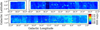 |
Fig. 1 RMS noise map of the 2° < ℓ < 40°, 56° < ℓ < 60°, and |b| < 1° region observed in B-configuration of the GLOSTAR survey. Each field is made by sampling on a size of 3′.25. High noise levels are found in the fields associated with bright emissions (the star-forming regions, H II regions, and other bright radio-emitting sources), observed at low declinations (close to the Galactic center), observed in bad weather conditions, and located at the edge area of the survey. High noise striping in Galactic Latitude is due to changes in observing conditions between scans. For B-configuration data of the “pilot region” of the GLOSTAR survey (28° < ℓ < 36°, |b| < 1°), see Dzib et al. (2023). |
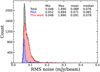 |
Fig. 2 Distributions of RMS noise level of the GLOSTAR B-configuration images (Fig. 1). The bin width is 0.002 mly beam−1. The red, blue and black histograms represent values determined for the region discussed here (2° < ℓ < 28°, 36° < ℓ < 40°, and 56° < ℓ < 60°), the pilot region (28° < ℓ < 36°) published in Dzib et al. (2023), and the combined area 2° < ℓ < 40°, 56° < ℓ < 60° area. The median RMS noise level is ~ 0.08 mJy beam−1 and 95% of the fields have a noise level < 0.13 mJy beam−1. |
3.4 Completeness
The completeness limit of the catalog can be investigated by running a source finder for added artificial point sources in the empty sky, that is, fields with few detections above 5 σ. The noise distributions vary spatially as outlined in Sect. 2.3, and hence to investigate the completeness limit of the whole survey, we chose several regions with a size of 0.5° × 0.5° that sampled all noise regimes such as high noise (~0.12 mJy beam−1), low noise (~ 0.06 mJy beam−1) and typical noise (~ 0.08 mJy beam−1). Then, one thousand artificial point sources are injected into each selected region. The position and peak flux densities of the injected sources are randomly produced from a uniform distribution, with a flux density range of 0.05–1.0 mJy. Following the same source extraction strategy described in Sect. 3.1, BLOBCAT was used to extract these added artificial sources. After 10 iterations of injection and extraction processes, the extracted results are compared with the injected source parameters to estimate the completeness. Figure 5 shows the fraction of the recovered artificial sources as a function of the peak intensity of the added artificial sources for fields with different noise levels. The completeness fraction varies among these fields, and fields with lower noise levels tend to reach the same completeness limit at lower flux density values. We find that a 95% completeness limit corresponds to ~0.35 mJy (red line in Fig. 5) for the best case of G22.5 and ~0.8 mJy (lime line in Fig. 5) for the worst case of G06.5. Typically, above ~0.6 mJy (i.e., the 7 σ-threshold detection limit for the high-reliability catalog in Sect. 3.3), the survey is 95% complete for point sources, as shown in the black line in Fig. 5 for all the selected fields.
3.5 Spectral index determination
As mentioned in Sect. 2, the GLOSTAR survey covers a wide bandwidth from 4 to 8 GHz, which was split into 9 sub-bands and each sub-band was imaged separately. We are thus able to determine the in-band spectral indices α by (1) extracting the peak flux density of each source within the sub-bands and (2) fitting the peaks to the formula Sv ∝ vα based on the scipy function curve_fit. The uncertainties in the peak flux densities are taken into account in the fitting process to estimate the uncertainty for the spectral index. When we are not able to extract the peak flux densities in all 9 sub-bands for some sources due to high noise or RFI in some sub-bands, the spectral indices are determined by fitting the remaining data points. More than 98% of the 7 σ sources have reliable data suitable for spectral fitting in at least five sub-bands. Figure 6 gives an example of the spectral index (α) fitting process for two bright sources with all 9 sub-bands and two faint sources with 5 and 6 sub-bands. With this strategy, we measured in-band spectral indices for 5430 sources in the 7σ-threshold catalog. The in-band spectral index of the 5430 sources ranges from −2.85 to 2.72, as listed in Table 5. The uncertainty in spectral index σα ranges from 0.01 to 2.63 with mean and median values of ~0.2 for both, and is strongly correlated with the S/N of the sources. Given that 97% of the 7-σ sources are compact with Yfactor < 2.0 (defined as the ratio between integrated flux density and peak flux density), the measured spectral index is not expected to be affected significantly by spatial filtering of the interferometer (due to missing short spacings).
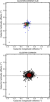 |
Fig. 3 Comparison of GLOSTAR astrometry with CORNISH and VLBI results. Top panel: offsets between GLOSTAR B-configuration positions (this work) and the positions of VLBI calibrators (black crosses, red filled ellipse) for 44 counterparts, and the offsets between CORNISH and VLBI calibrators for 75 counterparts (blue crosses, green filled ellipse). The VLBI calibrators have a (sub)milliarcsec positional accuracy (Petrov 2021). The median and standard deviation of the offsets are −0″.06 and −0″.11, suggesting a systematic positional difference of ≲0″.1 for the GLOSTAR and Very Long Baseline Array (VLBA) calibrators. Bottom panel: position offsets between the GLOSTAR B-configuration and CORNISH positions for 669 counterparts. The mean and standard deviation of the offsets are 0″.08 and 0″.16, suggesting a systematic positional difference of ≲0″.1 for the GLOSTAR and CORNISH. |
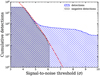 |
Fig. 4 Cumulative distribution of spurious sources (black histogram) and all detections (blue histogram) as a function of the S/N (1σ ~ 0.08 mJy), to estimate the spurious sources expected in the GLOSTAR survey. The red dashed line fitted to the negative detections indicates the expected spurious sources. Below 4.5 σ, the detections are dominated by spurious sources (occupying 93%) and the false detections decrease to 186 at 6.1 σ. Above 7 σ, fewer than 5 sources are expected to be false. |
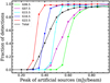 |
Fig. 5 Completeness fraction of recovered artificial sources as a function of the peak flux density of the total added artificial sources. The completeness of the selected fields with different typical noises are shown in different colors. The mean RMS values for the high, low, and typical noise regions are 0.12 mJy beam−1, 0.06 mJy beam−1, and 0.08 mJy beam−1, respectively. 95% completeness limit is reached at a flux density of ~0.35 mJy for the best case G22.5 (red line) and ~0.8 mJy for the worst case G06.5. Typically, the GLOSTAR survey in B-configuration is 95% complete to point sources at the ~0.6 mJy level (i.e., the chosen 7 σ threshold for the catalog in Sect. 3.3), as shown in black line for all the selected fields. See the completeness in Sect. 3.4 for details. |
GLOSTAR B-configuration catalog for 2° < ℓ < 28°, 36° < ℓ < 40 and 56° < ℓ < 60° and |b| < 1°.
3.6 Source classification
As outlined in the surveys of CORNISH (Purcell et al. 2013), THOR (Wang et al. 2018), and the GLOSTAR pilot (Dzib et al. 2023), the classification processes of the GLOSTAR sources were conducted based on multiwavelength counterparts and/or emission properties from the Galactic plane surveys such as the near-infrared (NIR) UKIDSS survey at J H K bands (Lucas et al. 2008), the GLIMPSE survey at 3–8 µm (Churchwell et al. 2009), the mid-infrared (MIR) WISE survey at 4–22 µm (Wright et al. 2010) and the MIPSGAL survey 24 µm (Carey et al. 2009), the far-infrared (FIR) Hi-GAL at 70–500 µm (Molinari et al. 2010), and the submillimeter (Submm) ATLASGAL survey at 870 µm (Schuller et al. 2009; Contreras et al. 2013; Csengeri et al. 2014; Urquhart et al. 2014, Urquhart et al. 2018, Urquhart et al. 2022). To search for counterparts, we adopt the beam size of these surveys as the search radius, such as 0.8″ for UKIDSS, 2″ for GLIMPSE, 6″ for WISE, and 6″ for MIPSGAL at 24 µm. We also carried out a visual inspection of the emission in different bands to look for association with extended structure. This was done by constructing three-color images from UKIDSS (red K-band 2.2 µm, green H-band 1.65 µm and blue J-band 1.2 µm), GLIMPSE (red 8.0 µm, green 4.5 µm, and blue 3.6 µm), and WISE (red 22.0 µm, green 12.0 µm and blue 4.6 µm) surveys, as well as images from the MIPSGAL, Hi-GAL, and ATLASGAL surveys.
The GLOSTAR sources are then classified as five types of candidates: H II regions, radio stars, planetary nebulae, extra-galactic sources, and others, using the criteria below:
H II regions: As ionized gas regions around massive stars are located in dense molecular clouds, H II regions are bright in the Submm, FIR, and MIR (Churchwell 2002; Anderson et al. 2012; Urquhart et al. 2013; Thompson et al. 2016; Yang et al. 2019). H II regions are also bright in the GLIMPSE three-color images due to emission from the associated polycyclic aromatic hydrocarbons (PAHs; Purcell et al. 2013; Tsai et al. 2009). Since they are deeply embedded in molecular clouds, young H II regions may still be dark or weak in NIR and even in some MIR bands (Hoare et al. 2012; Murphy et al. 2010; Yang et al. 2021). Therefore, radio sources associated with Submm and/or FIR emission are classified as H II regions.
Planetary nebulae (PNe): As ionized gas regions around young white dwarf stars (Bobrowsky et al. 1998), PNe and H II regions have similar emission properties at infrared and radio wavelengths (Anderson et al. 2012). Compared to H II regions, the spectral energy distributions (SEDs) of PNe tends to peak at shorter MIR wavelengths and fall off steeply at FIR (Anderson et al. 2012; Purcell et al. 2013), which often makes PNe undetectable in the submm range (Urquhart et al. 2013, Urquhart et al. 2018). Although some nearby PNe are detectable in the FIR (Hi-GAL) and the submm (ATLASGAL), their emission typically tends to be fainter at longer wavelengths (Anderson et al. 2012; Purcell et al. 2013). Since the SEDs typically peak in the MIR range, PNe tend to appear red in WISE and GLIMPS three-color images. Moreover, PNe are likely to be isolated point-like sources in GLIMPSE and UKIDSS images due to the absence of molecular clouds (Zhang & Kwok 2009; Hoare et al. 2012).
Radio stars: Both thermal and non-thermal radio emission from radio stars have been observed, that could arise from evolved OB stars, active stars, or active binaries, as discussec by Hoare et al. (2012). In the submm and FIR ranges, emssion from radio stars tends to be weak or absent. In the WISE, GLIMPSE, and UKIDSS three-color images of, radio stars tend to appear as blue and point-like sources (Hoare et al. 2012; Urquhart et al. 2013). Also, a GLOSTAR source is classified as a radio star if it has an NIR UKIDSS counterpart (offset <0″.8) that is suggested to be a star in the UKIDSS catalog (Lucas et al. 2008).
Extragalactic sources: extragalactic sources are usually not seen in the Submm, FIR, MIR, and NIR Galactic plane surveys (Hoare et al. 2012; Urquhart et al. 2013). Some of them are associated with very faint diffuse and/or point-like counterparts (offset < 0″.8) in the NIR UKIDSS, and the counterparts are classified as galaxies by Lucas et al. (2008).
Others: Radio sources that cannot be categorized as one of the above four types are classified as type “others”. One type in this class is the photodissociation region (PDR), namely, the interface between the ionized region and the molecular cloud, which are normally extended and bright at GLIMPSE, usually with weak or no emission in the FIR and Submm (Hoare et al. 2012).
An overall flow chart of the classification process is shown in Fig. 7 and the example sources are shown in Fig. 8. The presence or absence of emission at other wavelengths, along with the source classification is indicated in Table 3. In total, among the 5437 7 σ-threshold sources, we identify candidates of 251 H II regions, 784 radio stars, 282 PNe, 4080 extragalactic sources, and 29 Others. Among sources classified as the type “Others”, 11 are likely to be PDR region candidates (i.e., normally associated with extended emission at MIR, and only weak or no emission at FIR and SMM wavelengths; Hoare et al. 2012) while the rest are unidentified. As expected, most sources (~75%) are classified as extragalactic candidates.
To quantify the quality of the classification, we use a matching radius of 2″ for determining SIMBAD counterparts (Wenger et al. 2000), as outlined in the pilot paper of GLOSTAR (Dzib et al. 2023). Among the 5437 classified sources, 1010 are found to have SIMBAD counterparts, and more than half (542/1010) are classified as the SIMBAD type “Radio”. For the 251 H II regions candidates, 182 show SIMBAD counterparts, 95% (173/182) of which have SIMBAD types that are consistent with the expected properties of H II regions at different wavelengths, such as SIMBAD types of NIR/MIR/IR sources, molecular clouds, YSOs, star formation regions, dense cores, millimetric/submillimetric sources, and H II regions. Similarly, 166 PNe, 119 radio stars and 416 extragalactic sources have SIMBAD counterparts, with our classification being consistent with the SIMBAD type for 95% (158/166), 92% (111/119) and 97% (406/416) of PNe, radio stars and extragalactic sources respectively. In addition, the consistency of classification between this work and the CORNISH survey are 100% for H II regions and PNe, and 98% for extragalactic sources. This supports the validity of our classification criteria.
We noted that our classification criteria may misclassify a radio source if it displays the same multiband emission properties as the above source types but does not belong to any of these categories. For example, three extragalactic source candidates are found to be associated with three pulsars within a 1.1″ radius from the SIMBAD database, such as G016.8052− 01.0011 (e.g., PSR J1825-1446, Hobbs et al. 2004; Wang et al. 2020), G023.2721+00.2979 (e.g., PSR J1832-0827, Wang et al. 2001; Yao et al. 2017), and G023.3856+00.0631 (e.g., PSR J1833-0827, Tian et al. 2007; Jankowski et al. 2019). Therefore, further investigation is required to understand the nature of these candidates.
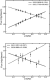 |
Fig. 6 Example of the peak flux as a function of the in-band frequency for bright sources (top panel) and faint sources (bottom panel). Each data point (circle or triangle) refers to the peak intensity at each sub-band, with the error of the peak measurement. The solid and dashed lines in the top panel show the best fit to the peak flux densities from 9 sub-bands for two bright sources: G020.0808−00.1354 (α = 1.1 ± 0.07) and G021.7700+00.8423 (α = −0.92 ± 0.04), respectively. The solid and dashed lines in the bottom panel present the spectral fitting of 5 and 6 sub-bands for two faint sources: GOll.9357+00.2871 (α = −1.7 ± 0.36) and G036.8880+01.0288 (α = 2.5 ± 0.6), respectively. |
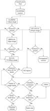 |
Fig. 7 Flowchart illustration of the radio source classification process. See the text of Sect. 3.6 for further details. |
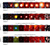 |
Fig. 8 Illustration of source types in the classification process of Sect. 3.6. From top to bottom: typical multiband images of a radio source classified as an H II region, a planetary nebula, a radio star and a extragalactic source. From left to right: three-colors composition image of UKIDSS (red = 2.2 µm, green = 1.65 µm, blue = 1.2 µm), three-color composition image of GLIMPSE (red = 8 µm, green = 4.5 µm, blue = 3.6 µm), three-color composition of WISE (red = 22 µm, green = 12 µm, blue = 4.6 µm), MIPSGAL 24 µm, Hi-GAL 70 µm, Hi-GAL 160 µm, Hi-GAL 250 µm, Hi-GAL 500 µm, and ATLASGAL 870 µm. The blue and white circle in the center show the position of radio emission. The FWHM beams of UKIDSS (0.8″), GLIMPSE (2″), WISE (6″ at 12 µm), MIPSGAL (6″ at 24 µm), Hi-GAL (6″–35″), ATLASGAL (19″) are indicated by the white circles with black hatched lines shown in the lower-left corner of each image. |
3.7 Clustered sources
Small clusters of radio sources are identified in the catalog using a friends-of-friends method (e.g., Purcell et al. 2013), that is, a source is associated with a cluster if it is located within 12″ of any other member in the catalog. Among the total of 5497 sources, 60 sources are likely to be artifacts or semi-ring-like fragmented components that have been removed from the catalog. 570 sources are found to be associated with 258 clusters. Among the 258 clusters, the majority (~84%; 216/258) harbors two radio sources. About 16% (42/258) clusters harbor more than two radio sources, with ~13% (33/258) harboring three radio sources and ~3% (9/258) having more than three sources. All cluster members of the B-configuration are usually detected as one source in the D-configuration (beam=18″) of the GLOSTAR with the D-configuration names from Medina et al. (2019) and Medina et al. (in prep.), being shown in Col. 12 of Table 3.
As mentioned in Sect. 2.2, the imaging process was restricted to have baselines of more than 50 kλ, due to which the survey is optimized to detect emission with angular size scales up to 4″. Hence, the extended sources with complex structures tend to be resolved and decomposed into multiple compact components, presented as group sources in clusters. To distinguish between adjacent but unrelated sources (top panel of Fig. 9) and resolved sources, we manually inspected each of the clustered sources. About 155 clustered members are associated with 56 clusters that are likely to trace resolved/fragmented sources, as shown in the middle-panel of Fig. 9. All the clustered sources that trace resolved sources are listed in Table 4. Some clustered sources show one or two semi-ring-like structures around the central compact bright component, suggesting that a single source that is fragmented as seen in the bottom panel of Fig. 9 and Fig. 3 of Dzib et al. (2023). The semi-ring-like fragments and the associated central compact component are regarded as one single radio source. It should be noted that the flux density is trustworthy only for the detected compact sources, and the flux of the extended sources, especially the fragmented cluster sources are underestimated due to the lack of short baselines. In the future, the combined B+D images from the GLOSTAR survey will be used for the reliable measurement of both compact and extended emissions of these resolved or fragmented sources. The imaging of the combined D+B configuration data of the entire survey is ongoing and will be published in a subsequent paper.
4 Results
We found 5497 sources above a 7 σ threshold in the region (2° < ℓ < 28°, 36° < ℓ < 40° and 56° < ℓ < 60) of GLOSTAR in B-configuration. We visually inspected the 7 σ detections and exclude 18 artifacts and 42 semi-ring-like fragmented components (see Sect. 3.7), giving a final catalog of 5437 sources. Among these 5437 sources, 251 are likely to be H II regions, 784 are candidates of radio stars, 282 are PNe candidates, and 4080 are likely to have extragalactic origins. The remaining 40 that cannot be classified into any of the above four types are regarded as “Other”, including 11 PDRs and 29 “unclear”, as mentioned in Sect. 3.6 and listed in Table 3.
4.1 Catalog description
The catalog contains 17 columns for each source, as presented in Table 3. Columns 1–8 are determined or derived by the source finder tool BLOBCAT as described in Sect. 3.1, and correspond to the Galactic name of the GLOSTAR source, Galactic longitude ℓ and latitude b, the S/N, peak flux density Speak and its uncertainty ∆Speak, integrated flux density Sint and its uncertainty ∆Sint. The Yfactor (defined as the ratio between the integrated flux density and the peak flux density, Yfactor = Sint/Speak) is listed in Col. 9. The source effective radius Reff, determined by the pixel size and the total number of pixels composing the source as outlined in Sect. 3.1, and the spectral index α, obtained by fitting the peak flux densities of the sub-band images (see Sect. 3.5), are presented in Cols. 10–11. Column 12 gives the corresponding D-configuration name from the GLOSTAR survey (Medina et al. 2019, and in prep.), which includes cluster sources as discussed in Sect. 3.7. The information about the presence or absence of counterparts in the NIR, MIR, FIR and Submm (see Sect. 3.6) are displayed in Cols. 13–16. Column 17 gives the source classification based on the multiwavelength properties as outlined in Sect. 3.6. All the columns are displayed in Table 3 for a small portion of the catalog, with full catalog available at the CDS and the GLOSTAR website1.
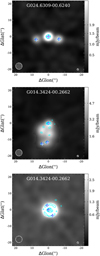 |
Fig. 9 Example of cluster sources in three cases. Top panel: the cluster sources in normal case. Middle-panel: example of clusters consists of over-resolved sources are listed in Table 4. Bottom panel: example of clusters with semi-ring-like fragments. In this case, the sources with semi-ring-like structures have been removed from the catalog. The positions of 7σ cluster sources are noted by blue and white pluses. The Galactic name of each figure refers to the source in the center position. The cyan contours are emission from B-configuration images (this work), starting at 5σ with 5σ increment. The background of each image presents the B+D configuration of GLOSTAR (Brunthaler et al. 2021). The FWHM beams of B (1″.0) and B+D configuration (4″.0) are presented by the white circles in the lower-right and lower-left corners of each image. |
GLOSTAR D-configuration sources that are detected as fragmented sources (e.g., multiple components or over-resolved of an extended source) in the B-configuration images.
4.2 Galactic distribution
To show the Galactic distributions for the whole B-conflguration catalog, we combined our work with the catalog published in Dzib et al. (2023). Figure 10 presents the distributions of GLOSTAR sources as a function of Galactic Longitude (ℓ) and Latitude (b). The full sample, the extragalactic, and Galactic sources are shown in light purple, purple, and dark purple, respectively.
As shown in the upper-panel of Fig. 10, the number of sources per 0.l°latitude bin increase gradually toward zero latitude for the total sample (light purple), which is due to the expected peak at b ~ 0.0° of the Galactic sources (dark purple). The extragalactic sources (purple) show a relatively flat distribution with Galactic latitude, which is also seen in Hoare et al. (2012) for the CORNISH survey. We note that the distribution of Galactic sources in latitude is slightly asymmetric and skewed toward b > 0°, which is also seen for the Galactic SNR distribution in GLOSTAR (Dokara et al. 2021) and in THOR (Anderson et al. 2017). This asymmetry is supported by a Shapiro–Wilk test of the Galactic source distribution in latitude that gives a statistical confidence of p-value ≪ 0.001. We found that the source counts of H II regions peaks at latitude b ~ 0.0°, as noted by Urquhart et al. (2013), while the distributions of radio stars and planetary nebulae are relatively flat along latitude from −1.0° to 1.0°.
The lower-panel of Fig. 10 shows the source counts in 2° bins of Galactic longitudes. The source counts are seen to have peaks at certain longitudes such as ℓ ≈ 10° and ℓ ≈ 26°. These correspond to locations of star formation regions such as W31, SFCl-4 (Thompson et al. 2006; Murray 2011) and W42 (Gao et al. 2019; Liu et al. 2019; Feng et al. 2021). The Kolmogorov–Smirnov (K-S) tests between the Galactic sources and the extragalactic sources give a statistical confidence p-value ≪ 0.001, which confirms that their distributions are significantly different in both Galactic longitude and latitude. The source count of extragalactic sources is seen to drop in regions with high noise such as |b| > 0.9° at the survey edges and 2°< ℓ < 8° at low declination, as shown in Fig. 1. Considering the high noise at 2°< ℓ <8°, the number of extragalactic sources per 2° longtitude bin still decrease gradually toward longitude zero, which is also seen in the distribution of non-classified sources with extragalactic origin in THOR survey (Fig. 13 of Wang et al. 2018). The number of Galactic sources per 2° longtitude bin increase toward longitude zero, which is also seen for the distributions of the resolved sources with galactic origin in the CORNISH survey (Fig. 18 of Purcell et al. 2013) and the Galactic sources (PNe and HII regions) in the THOR survey (Fig. 13 of Wang et al. 2018).
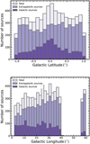 |
Fig. 10 Distribution of 6894 GLOSTAR B-configuration 7 σ–threshold sources as a function of Galactic Latitude (upper panel) and Longitude (lower panel) for the B-configuration catalog, including the catalog of this work (2° < ℓ < 28° 36° < ℓ < 40 and 56° < ℓ < 60 and |b| < 1°), as listed in Table 3 and the published pilot catalog (28° < ℓ < 36° and |b| < 1°) in Dzib etal. (2023). The bin sizes are 0.1° and 2.0° for the upper and lower panel, respectively. The blank region in Galactic longitude 40° < ℓ < 56° is not covered by the GLOSTAR survey in B-configuration. |
4.3 Source properties
In this section, we present the source properties for the high reliability (7 σ–threshold) catalog. Table 5 displays a statistical summary of the source properties for the total catalog in Table 3, the extragalactic sources, and the Galactic sources. The typical values of flux density, effective radius, and spectral index of the sources in the catalog are Sint ~ 1.0 mJy, Reff ~ 0″.8, and α ~ −0.52, indicating that the detected sources are typically compact and weak, and are dominated by extragalactic sources with non-thermal emission.
Summary of source properties of the 7 σ–threshold catalog.
4.3.1 Source effective size
Figure 11 shows the source counts as a function of source effective sizes (see Sect. 3.1) for the high reliability catalog of GLOSTAR B-conflguration (light purple), with the extragalactic and Galactic sources being shown in purple and dark purple respectively. As shown in Table 5, the effective radius of the sample ranges from 0.45″ to 2.69″, with a mean and median value of 0.86″ and 0.80″ respectively. As expected, the Galactic sources have larger sizes with a higher mean Reff compared to the extragalactic sources, and the two distributions are significantly different as suggested by the K–S test (p-value ≪ 0.001).
The effective source sizes are calculated from the total number of pixels comprising each source obtained from the BLOBCAT software (see Sect. 3.1). As discussed for the THOR survey (Bihr et al. 2016; Wang et al. 2018), the effective radius is not a good parameter to distinguish between resolved and unresolved sources. Hence, we use the parameter Yſactor (i.e., Sint/Speak in Table 3), namely, the ratio between the integrated (in units of mJy) and peak flux density (in units of mJy beam−1), to divide sources into three subsamples: extended sources (Yfactor > 2.0), compact sources (1.1 < Yfactor ≤ 2.0) and unresolved/point-like sources (Yfactor ≤ 1.1). This is identical to what was used in the pilot region of the GLOSTAR B-configuration (Dzib et al. 2023) and the D-configuration (Medina et al. 2019), as well as in previous work (e.g., Bihr et al. 2016; Yang et al. 2019). As expected, the majority of the detected sources (97% = 5255/5437 with Yfactor ≤ 2) are compact (2053 with 1.1 < Yfactor ≤ 2.0) and unresolved/point-like sources (3202 with Yfactor ≤ 1.1), due to the fact that the images are optimized for detection of compact emission (see Sect. 2.2). In the above three categories of unresolved, compact, and extended sources, 79%, 73%, and 32% of them are extragalactic sources candidates, respectively. About 98.6% of the extragalactic sources and 91% of the Galactic sources are compact and unresolved with Yfactor ≤ 2.0. The remaining 1.4% of extragalactic sources are extended with Yfactor > 2.0, which are expected to be associated with radio galaxy lobes, while the extended Galactic sources (9% of the Galactic sources) are found to be preferentially associated with H II regions and PNe.
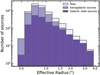 |
Fig. 11 Distribution of source effective radius for the 6894 sources in the 7 σ–threshold catalog of this work (Table 3) and the published pilot catalog in Dzib et al. (2023). |
4.3.2 Peak and integrated flux density
The peak and integrated flux densities are obtained as outputs from the source extraction tool, BLOBCAT (see Sect. 3.1). Figure 12 shows the distributions of peak and integrated flux density for the high reliability catalog (light purple), the extragalactic sources (purple), and the Galactic sources (dark purple). The decline in the source count for flux densities below 0.65 mJy is due to the non-uniform noise distribution and the resulting variation in the 7 σ detection limit over the survey region.
It is to be noted that there is a significant population of unresolved sources with Yfactor < 10, which means that their integrated flux densities (Sint) are lower than their peak intensities (Speak). While for most of the sources, the integrated flux densities and the peak intensities are still consistent within 3σ, there are a few sources where the discrepancy is significant. This could happen when the unresolved sources are (1) not fitted with enough pixels by BLOBCAT (i.e., fitted area less than beam); (2) located in negative side lobes from nearby bright sources; and (3) not cleaned properly. These are also seen in other survey catalogs generated using BLOBCAT, such as that of THOR (Bihr et al. 2016; Wang et al. 2018) and the GLOSTAR pilot region (Dzib et al. 2023; Medina et al. 2019). Therefore, for these unresolved sources with a Yfactor < 1.0, we used their peak flux densities for further analysis discussed in the following sections.
4.3.3 Spectral index
Figure 13 shows the distribution of spectral index for the full high reliability sample of this work (light purple), extragalactic (purple), and Galactic sources (dark purple). The measured in-band spectral index of this work is consistent with that measured in THOR for compact sources that are detected in both surveys, as discussed later in Sect. 5.1.3. The K-S test of the spectral index between the Galactic sources and the extragalactic sources (p-value ≪ 0.001) suggests that they are significantly different.
The spectral index is a common and useful tool for distinguishing between thermal and non-thermal radio emission, broadly corresponding to positive and negative spectral indices, respectively. The catalog is dominated by non-thermal radiation, as it includes 74% of sources with α < −0.1. The spectral index of extragalactic sources (purple) and the total sample (light purple) peaks at α ~ −0.6, as seen in the pilot paper (Dzib et al. 2023). Among the 4080 extragalactic sources, about 77% have negative spectral indices with α < −0.1, while 23% show spectral indices from thermal emission with α > −0.1. The spectral index of Galactic sources (dark purple in Fig. 13) peaks at ~ −0.2, with 67% having α < −0.1 (mainly radio stars) and the remaining 33% having α > −0.1 (mainly H II regions and planetary nebulae). This shows that the radio emission from both Galactic and extragalactic sources is dominated by non-thermal radiation. It is to be noted that the uncertainty in the spectral index is strongly correlated with the logarithm of S/N, with a correlation coefficient of ρ = −0.89 and p-value ≪ 0.001. Hence, the in-band spectral indices of weak sources just above the detection limit of 7 σ are less reliable, with their being some cases of two adjacent pixels having very different spectral indices. A similar observation was made by Rosero et al. (2016) for weak and compact radio emission in high-mass star-forming regions.
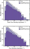 |
Fig. 12 Distributions of peak (upper panel) and integrated (lower panel) flux density for the 6894 7 σ − threshold sources of GLOSTAR B-configuration, including Table 3 and the published pilot catalog in Dzib et al. (2023). |
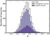 |
Fig. 13 Distribution of spectral index α for the 7 σ −threshold catalog of the GLOSTAR B-configuration, including Table 3 and the published pilot catalog in Dzib et al. (2023). |
5 Discussion
5.1 Comparison with other radio surveys
The comparison between GLOSTAR and other radio surveys allows us to discuss the consistency of peak and integrated flux densities, and positions of the detected sources. Due to the differences in spatial filtering, angular resolution, and uυ coverage, the comparisons of radio properties are valid for compact sources detected in these surveys. In this section, we compare the properties of compact sources in our catalog with other surveys such as CORNISH (e.g., Hoare et al. 2012; Purcell et al. 2013), MAGPIS (e.g., White et al. 2005; Helfand et al. 2006), and THOR (e.g., Bihr et al. 2016; Beuther et al. 2016; Wang et al. 2018).
5.1.1 The CORNISH survey
The CORNISH survey has the most similar observation setup and sky coverage to the B-configuration of the GLOSTAR survey, making it an excellent resource for a comprehensive inspection of the source properties in this study. CORNISH (Hoare et al. 2012; Purcell et al. 2013) used the VLA in B and BnA configurations at 5 GHz to conduct a Galactic plane survey from 10° < ℓ < 65° and |b| < 1°, with a resolution of 1.5″ and a median RMS noise of ~ 0.4 mly beam−1. A total of 2638 high-reliability CORNISH sources are detected above the 7σ limit (~2.5 mJy beam−1), containing extended emission on scales no greater than 14″. Compared to CORNISH, GLOSTAR in B-configuration has a similar angular resolution of 1.0″ and better sensitivity of ~ 0.08 mly beam−1 (i.e., the 7σ detection limit ~0.56 mJy beam−1), but a poorer sampling of extended emission with the images being mostly insensitive to emission on scales >4″ (see Sect. 2.2). Despite their differences in the uυ coverage, the properties of compact and unresolved sources are expected to be common in both catalogs. The comparison between GLOSTAR and CORNISH for the pilot region (28° < ℓ < 36°, |b| < 1°) has discussed in Dzib et al. (2023).
Within the overlap region of this work (10° < ℓ < 28°, 36° < ℓ < 40°, 56° < ℓ < 60°, and |b| < 1°), CORNISH detected 1210 high-reliability sources above 7σ, including 742 compact sources (defined as sources with angular sizes ≤ 1.8″ in Purcell et al. 2013). In the overlap region, GLOSTAR detected 4381 sources above 7σ, highlighting the improvement in sensitivity. Among these 742 compact CORNISH sources, we find a match of 669 GLOSTAR sources, using a circular matching threshold of 1.8″, giving a match rate of ~90%. The match rate is similar (90%=259/290) even if we only consider sources that are unresolved by CORNISH (i.e., sizes ≤ 1″.5). In spite of the improved sensitivity of the GLOSTAR survey, there are 73 sources that are detected by CORNISH but not by GLOSTAR. An examination of the location of these sources reveals that about 54% (40/73) are located at the survey edges with |b| > 1.0 that are not covered by GLOSTAR. The remaining sources are likely to be variable radio sources as discussed later in Sect. 5.6. The catalog discrepancies between CORNISH and GLOSTAR have also been discussed in the GLOSTAR pilot papers by Dzib et al. (2023) and Medina et al. (2019).
Figure 14 shows the comparison of flux densities of CORNISH and GLOSTAR for the 669 compact sources that have been detected in both surveys. We measured a mean± standard deviation of the flux ratio of 1.14 ± 0.3, demonstrating a good agreement between the two surveys. The consistency of flux measurements between CORNISH and GLOSTAR was also seen in the D-configuration catalog of the pilot region (see Fig. 11 in Medina et al. 2019). Because CORNISH (beam=1″.5) and GLSOTAR (beam=1″.0) have similar angular resolutions, we have also used these compact matching sources to infer the astrometric accuracy of the GLOSTAR survey, indicating a position uncertainty of ≲ 0″.1 for this catalog (see Fig. 3 and Sect. 3.2 for details).
Among the compact sources detected in both surveys, CORNISH has classified 17 sources as H II regions, 32 as planetary nebulae, and 577 as extragalactic sources. Among these CORNISH sources with types, GLOSTAR found all 17 H II regions and 32 planetary nebulae, as well as 569 extragalactic sources. This gives a classification match rate of 100% for H II regions and PNe, and 98% for extragalactic sources. This demonstrates a high level of agreement in classification between the two surveys.
5.1.2 The MAGPIS survey
The Multi-Array Galactic Plane Imaging survey (MAGPIS 4) observed the Galactic plane at 5 GHz between −10° < ℓ < 42° and |b| < 0.4° (White et al. 2005) and at 1.4 GHz between 5° < ℓ < 32° and |b| < 0.8° (Helfand et al. 2006), with a resolution of 6″ and a median 1σ noise of ~0.29 mJy beam−1. The detection threshold of MAGPIS was chosen to be ~5.5 σ (~ 1.4 mJy beam−1) compared to 7σ (~0.56 mJy beam−1) for GLOSTAR in this paper. Due to the differences in uv coverage, we only examine the properties of compact and unresolved sources in the catalogs of MAGPIS and GLOSTAR B-configuration (including this work and Dzib et al. 2023).
For the 5 GHz catalog in White et al. (2005), within the overlapping region of the GLOSTAR B-configuration (2° < ℓ < 40° and |b| < 0.4°), MAGPIS detected 2345 sources above 5.5 σ with angular size measurements, including 935 compact sources (defined as sources with angular sizes < 6″ in MAGPIS; White et al. 2005). In the same region, GLOSTAR detected 6216 sources above 7σ. Among the 935 compact MAGPIS sources, we find a match of 684 GLOSTAR sources above 5σ using a matching radius of 5″. The remaining sources that are detected by MAGPIS but not by GLOSTAR are extended with angular sizes greater than 4″ (i.e., the largest angular scale structure detected by GLOSTAR in B-configuration). Due to the differences in the adopted detection thresholds and the uv coverage between MAGPIS and GLOSTAR, among the 684 5σ matches, 663 are above 7σ in the high-reliability catalog of GLOSTAR. From the top panel of Fig. 15, we can see that the measured flux densities of the unresolved sources (i.e., Yfactor < 1.1) in GLOSTAR and MAGPIS are in good agreement, as was also seen in Medina et al. (2019) for the D-configuration catalog of the pilot region. The outliers that have Yfactor < 2 could be from the variable radio source sample such as G031.0777+00.1703 in Dzib et al. (2023) which is the outlier point located at the bottom-right of Fig. 15. The extended sources with Yfactor > 2 are responsible for the outliers that show higher flux densities in MAGPIS compared to GLOSTAR, which is mainly attributed to differences in uv coverage between the two surveys.
For the 1.4 GHz catalog in Helfand et al. (2006), within the overlapping region (5° < ℓ < 32° and |b| < 0.8°), MAGPIS detects 3149 sources above 5 σ, 1153 of which are compact with angular sizes < 6″sources. Using a matching radius of 5″, GLOSTAR detects 860 sources above 7 σ at 5 GHz. To compare the flux densities at the same observing frequency with MAGPIS 1.4 GHz, we extrapolated the GLOSTAR 5 GHz flux densities to the 1.4 GHz flux densities according to the spectral indices of GLOSTAR catalog. To make the 1.4 GHz extrapolated flux densities reliable, we select the 484 compact sources that have low uncertainties in their spectral indices (i.e., σα < 0.2, where 0.2 is the typical value of σα as outlined in Sect. 3.5). The bottom panel of Fig. 15 shows the comparison of 1.4 GHz flux densities of MAGPIS and GLOSTAR for the 484 compact sources detected by both surveys. This suggests that the extrapolated 1.4 GHz flux densities from GLOSTAR agree with the 1.4 GHz MAGPIS fluxes. Considering the differences in uv coverage and the observing frequency, the flux measurements of the two surveys are consistent.
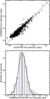 |
Fig. 14 Comparison of flux densities between GLOSTAR and CORNISH. Top panel: the comparison of flux densities for 669 compact sources detected by both CORNISH and GLOSTAR catalogs. The error bar of each point shows the uncertainty of flux. Bottom panel: the histogram of the flux density ratios of compact sources between CORNISH and GLOSTAR. The black line displays the Gaussian fit to the histogram. The dashed line presents the mean value of the distribution, with mean and standard deviation of the flux ratio from the Gaussian fit are 1.14 and 0.3, respectively. |
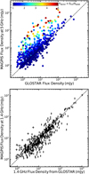 |
Fig. 15 Comparison of flux densities between GLOSTAR and MAGPIS. Top panel: The comparison of measured flux densities for 663 MAGPIS compact sources at 5 GHz (White et al. 2005) common to GLOSTAR. These compact sources are defined as sources with angular sizes < 6″ in MAGPIS. The dashed line means the flux densities are the same in MAGPIS and GLOSTAR. At the top, we show the color bar for the Yfactor (defined as Sint/Speak) of the GLOSTAR detections, indicating the emission of sources in the GLOSTAR image are unresolved (defined as Yfactor < 1.1 in Sect. 4.3.1), compact (1.1 < Yfactor < 2.0) or extended (Yfactor > 2.0). Bottom panel: The comparison of flux densities of 484 compact MAGPIS at 1.4 GHz that are also detected by GLOSTAR at 5 GHz. The 1.4 flux densities from GLOSTAR is extrapolated from the 5 GHz flux densities and spectral indices of the GLOSTAR catalog. |
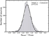 |
Fig. 16 Distribution for the difference (αBconf − αTHOR) in the measured spectral indices for 1390 compact THOR sources common to GLOSTAR in B-configuration. The black solid line means the Gaussian fit for the distribution, giving a mean value of −0.04 ± 0.03 (the error of the mean is from the Gaussian fit) and a standard deviation of 0.78. |
5.1.3 The THOR survey
The THOR survey (Bihr et al. 2015, Bihr et al. 2016; Beuther et al. 2016; Wang et al. 2018) observed HI, OH, recombination lines, and continuum of the Galactic plane between 14.5° < ℓ < 61.4° and |b| < 1.25°, using the VLA in C-configuration at 1–2 GHz. The continuum images of THOR have a 1 σ noise level of 0.3–l.0 mJy beam−1 and a typical angular resolution of ~25″. The detection threshold of THOR is set as 5 σ, and a total catalog of 10387 sources is detected above the threshold. Given the large differences in the observation setup and uv coverage between THOR and GLOSTAR in B-configuration, we can only roughly discuss the similarities and differences between the two surveys. The comparison between GLOSTAR and THOR for the pilot region (28° < ℓ < 36°, |b| < 1°) can be found in Dzib et al. (2023).
Within the region of overlap between THOR and the GLOSTAR area presented in this work (14.5° < ℓ < 28°, 36° < ℓ < 40°, 56° < ℓ < 60° and |b| < 1.0°), THOR detected 4083 sources above 5σ as reported in Wang et al. (2018). In the overlapped region, GLOSTAR detected 3650 sources above 7σ detection level. Using a matching radius of 5″, we found 2363 common sources above 5σ and 2001 matches above 1σ in the GLOSTAR survey. Among these 7σ matches, 1764 are regarded as point sources in the THOR survey, 1390 of which have had spectral indices measured by both surveys. Figure 16 shows the distribution of the difference in the measured spectral index (αBconf − αTHOR) for these sources. The mean difference in spectral index between the two surveys is −0.04 + 0.03 (the error is estimated from a Gaussian fit to the distribution in Fig. 16), with a standard deviation of 0.78. The mean value reduces to −0.02 if the matched sources are also compact (Yfactor < 2) in GLOSTAR, and down to zero if the sample is restricted to be sources that are classified as extragalactic in Sect. 3.6. The spectral indices of compact sources measured in the two surveys are thus consistent. A similar result was found in the catalog of the pilot region (Dzib et al. 2023). Figure 16 also shows the presence of a number of sources that have significant differences in spectral index measurement between THOR and GLOSTAR, such as abs(αBconf − αTHOR) > 2. This could be due to: (1) the big differences in beam sizes of THOR (~25″) and GLOSTAR in B-configuration (~1″); (2) the measurement uncertainties of spectral index measured in THOR (Bihr et al. 2016) and in this work; (3) a turnover in the radio spectra between THOR and GLOSTAR.
Among the 1764 7σ compact matches, only 130 sources have been classified by THOR, including 45 H II regions and 57 PNe candidates. The classification in THOR is consistent with our classification for 38 out of the 45 H II regions and 53 out of the 57 PNe. This gives a classification match rate of 84% (38/45) for H II regions and 92% (53/57) for PNe. Differences in classification can be caused by the differences in the matching radius used for comparison in IR surveys between the two surveys, as discussed in the GLOSTAR catalog paper of the pilot region (Dzib et al. 2023).
5.2 H II region candidates
As discussed in Sect. 3.6, radio sources with submm and FIR emission are classified as H II region candidates. These H II region candidates trace radio emission in star formation regions (SFR). In this paper, we identified 251 H II region candidates5 Among these H II regions, 138 are identified/detected by previous work using the CORNISH, THOR, and the SIMBAD database. Therefore, 113 H II regions are newly identified in this work.
The H II region candidates of this work are compact and show a mean effective angular size of 1.2″, ranging from 0.55″ to 2.69″. This indicates that the majority of them belong to the category of the most compact H II regions (e.g, Hoare et al. 2007), such as hyper-compact H II (HC H II) regions and ultra-compact H II (UC H II) regions (e.g., Kurtz 2005; Yang et al. 2021; Liu et al. 2021; Patel et al. 2023). Combined with the compact H II region candidates in Table 1 of Dzib et al. (2023), we obtain a sample of 390 H II region candidates in GLOSTAR B-configuration.
The distribution of the spectral index α for the 390 H II region candidates is shown in the top panel of Fig. 17, and α ranges from −3.70 and 2.96, with a mean value of −0.53. Considering the uncertainties of the spectral indices σα as outlined in Sect. 3.5, we choose to discuss the H II region candidates that have a reliable spectral index, that is, σα < 0.2 (where 0.2 refers to the typical value of σα in the catalog). This gives a sample of 183 H II region candidates, with −2.33 < α < 1.58, as the hatched histogram shown in the top panel of Fig. 17. Previous studies have reported positive and negative spectral indices for H II region candidates in the CORNISH survey (Kalcheva et al. 2018) and H II region candidates in the GLOSTAR pilot region (Dzib et al. 2023).
Theoretically, the radio continuum emission of an H II region is thermal and has a spectral index α (Sv ∝ vα) varying from +2 (optically thick) at low frequency to −0.1 (optically thin) at high frequency. We use the spectral index α to divide H II region candidates into two subsamples: the α < −0.1 group (66% = 120/183) and the α > −0.1 group (34% = 63/183), with mean values of α ~ −0.7 and α ~ 0.6, respectively. Considering 2 times of the uncertainties in spectral index (2 σα) for the two samples, the fraction of the α > −0.1 sample increase to about 50%. The mean spectral index of 0.6 for the α > −0.1 group refers to the thermal emission from H II regions, which is similar to the mean of α ~ 0.6 observed at 5 GHz for the young H II regions (HC H II and UC H II) sample in Yang et al. (2019) who suggest the existence of H II regions with a mix of optically thin and thick components along the line of sight.
Intriguingly, the majority (~66%) of the sample belongs to the α < −0.1 group with a mean spectral index of −0.7, which indicates that a substantial portion of radio emission in these H II region candidates is non-thermal. A number of observational studies have reported the existence of H II regions with a mixture of thermal and non-thermal radiation (e.g., Wang et al. 2018; Meng et al. 2019; Padovani et al. 2019) and dominated nonthermal emission (e.g., Wilner et al. 1999; van der Tak & Menten 2005; Rosero et al. 2019). The H II region with radio continuum α < −0.5 are considered to be dominated by non-thermal emission (Kobulnicky & Johnson 1999). Considering that 74 out of the 120 H II region candidates have α < −0.5, we suggest these are dominated by non-thermal emission, while the remaining 46 candidates with −0.5 < α < −0.1 are likely to be associated with a mixture of thermal and non-thermal radiation.
Given that the H II region candidates are identified by radio emission in star formation regions (see Sect. 3.6), it is possible that the non-thermal radio emission originates from the processes such as radio jets, shocks and outflows from highmass (van der Tak & Menten 2005) and low-mass stars (Gómez et al. 2002). We find that the α < −0.1 group is more likely to be located in clusters (see Sect. 3.7) and be associated with molecular outflows in Yang et al. (2018, Yang et al. 2022a) compared to the α > −0.1 sample, implying that the non-thermal emission arises from localized spots that are seen only when the large scale emission is filtered out by the interferometer. From Fig. 17, we can see that the α < −0.1 sample shows significantly lower values of peak flux density compared to the α > −0.1 sample, indicating that the α < −0.1 sample are relatively compact and weak. Thus, these clustered non-thermal emission spots are likely to be radio jets and outflows located in the vicinity of H II regions and in star formation regions (e.g., Wang et al. 2012; Purser et al. 2016; Rosero et al. 2016; Liu et al. 2017; Qiu et al. 2019). This is consistent with the findings of Wang et al. (2022) who suggested that most of the radio sources in the Cygnus region are radio jets and winds originating from massive young stellar objects. In Fig. 18, we displayed an example of the two H II region candidates (G024.7897 and G024.7888) that shows positive and negative in-band spectral index derived by fitting the 8 sub-bands radio images of the GLOSTAR. The H II region candidate G024.7897 (Yfactor = 1.02) with α = 1.43 ± 0.02 is supposed to be a “real” H II region, which shows extended green emission (as defined by Cyganowski et al. 2008) in Fig. C.1, and is associated with a maser-emitting UC H II region in Hu et al. (2016). In contrast, the nearby H II region candidate G024.7888 (Yfactor = 1.97) with α = −0.55 ± 0.04 is likely to be the non-thermal emission from radio jets or outflows in massive star-forming regions. Some of the sources in the catalog were confirmed as non-thermal sources through VLBI observations by Dzib et al. (2016). We note that there are many H II regions like G024.7897 that are surrounded with at least one non-thermal source like G024.7888, as shown in Fig. C.1, which is consistent with the findings in Gómez et al. (2002) who detected a cluster of non-thermal sources around a young and compact UC H II region with VLA observations and suggested these non-thermal clusters are originated from low-mass, pre–main-sequence stars.
In summary, from the α > −0.1 sample, we confirm the existence of the H II regions with a mixture of optically thin and thick thermal emission components. From the α < −0.1 sample, we find that a large fraction of compact H II region candidates are associated with non-thermal emission, suggesting that these candidates can be radio jets, winds and outflows from high-mass and low-mass young stellar objects. This further indicates that there is a significant amount of relativistic electrons that exist in star-forming regions. Further investigation is required to confirm the nature of non-thermal emissions in massive star-forming regions.
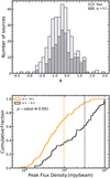 |
Fig. 17 Distributions of spectral index and peak flux densities of HII region candidates in GLOSTAR B-configuration. Top panel: the histogram of the measured spectral index for the total 390 H II region candidates of GLOSTAR B-configuration. The hatched histogram represents the 183 candidates with σα < 0.2. The bin size is 0.25. The 183 candidates are divided into two subsamples: (1) 120 H II regions with α and (2) 63 H II regions with α > −0.1, indicating non-thermal and thermal emissions, respectively. Bottom panel: the cumulative distribution of the peak flux densities for the α < −0.1 sample (orange line) and the α > −0.1 sample (black line). The orange and black vertical dashed lines show the mean values of 9.5 mJy beam−1 and 31.6 mJy beam−1 for the two subsamples, respectively. |
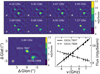 |
Fig. 18 Example of two H II region candidates with positive and negative in-band spectral index, as discussed in Sect. 5.2. The top two rows show the 8 sub-bands of the GLOSTAR image. The bottom-left panel shows the averaged image at 5.8 GHz used to extract the source, and the bottom-right panel shows the in-band spectral index fitting for the two compact H II regions candidates: the solid line for G024.7897 (Yfactor = 1.02) with α = 1.43 ± 0.02 and the dashed line for G024.7888 (Yfactor = 1.97) with α = −0.55 ± 0.04. The FWHM beam of GLOSTAR in B-configuration (1.0″) is indicated by the white circles in the lower-left corner of each image. There is a clear trend that the fluxes increase and decrease as the increasing frequencies in the sub-bands for G024.7897 and G024.7888 respectively. |
5.3 Planetary nebula candidates
We identified 282 planetary nebulae (PNe) based on the classification process described in Sect. 3.6. Among these, 155 are identified/detected by previous work and 127 PNe are new detections.
These PNe candidates are compact and their effective size range from 0.53″ to 2.46″ with a mean and standard deviation of 1.0″ and 0.3″ respectively. About 54% of the sources have effective sizes less than 1.0″. The in-band spectral indices α of the PNe candidates range from −2.75 to 1.9, with a mean value of −0.52. Combining with the 68 PNe candidates identified in the Table 1 of Dzib et al. (2023) for the pilot region, we obtained a sample of 350 PNe candidates for the GLOSTAR B-configuration catalog.
As in H II regions, from the 162 PNe candidates with σα < 0.2, two subsamples are obtained: (1) PNe candidates with α < −0.1 (62% = 100/162) and (2) PNe candidates with α > −0.1 (38% = 62/162). This is similar to observations from previous surveys such as CORNISH (Irabor et al. 2018) and the pilot region of GLOSTAR (Dzib et al. 2023), who found that PNe were found with radio emission showing both positive and negative spectral indices. This suggests that both thermal and non-thermal emission components are associated with PNe candidates. Theoretically, PNe are thus expected to have radio continuum from thermal free-free emission with −0.1 < α < 2 (e.g., Gómez et al. 2005; Tafoya et al. 2009; Qiao et al. 2016). Thus, similar to the H II region candidates, the PNe candidates with spectral index greater than and less than −0.1 are expected to be associated with thermal and non-thermal emission, respectively.
Observationally, a low spectral index threshold of α < −0.5 between 1 GHz and 20 GHz was suggested to identify non-thermal emission from planetary nebulae detected in the AT20G survey (i.e., the Australia Telescope 20 GHz survey, Chhetri et al. 2015). Planetary nebulae with both non-free-free emission components (e.g., Casassus et al. 2007; Irabor et al. 2018) and even non-thermal dominated emission (e.g., Suárez et al. 2015; Cerrigone et al. 2017; Anglada et al. 2018) have been reported before. Non-thermal emission is found in young PNe that are associated with masers (Cohen et al. 2006) or that are in the formation stage (Cerrigone et al. 2017). In our sample of sources with α < −0.1, 59 PNe candidates have α < −0.5 and thus are likely to be dominated by non-thermal emission, while the remaining 41 PNe candidates with −0.5 < α < −0.1 are thought to have both thermal and non-thermal components. The α < −0.5 candidates show significantly lower Yfactor and flux densities compared to sources of the α > −0.5 sample. This suggests that the α < −0.5 sources are denser and weaker and thus likely associated with radio jets. In short, we found a large fraction of PNe are associated with compact non-thermal emissions likely from radio jets, suggesting that these PNe candidates are very young or in the formation stage.
5.4 Extragalactic source candidates
In this paper, we identified 4080 extragalactic sources based on the classification process outlined in Sect. 3.6. This is consistent with the expected number of ~4137 estimated from the FIRST survey (White et al. 1997) and ~4100 calculated from Eq. (A2) of Anglada et al. (1998) using the 5 GHz source counts of Condon (1984) and the typical detection level (~ 0.6 mJy beam−1) of this work. Among these extragalactic sources, 1905 have been identified/detected previously in the CORNISH and THOR surveys and the SIMBAD database. Therefore, 2175 extragalactic sources are newly identified by this work.
Combining with the 1157 extragalactic source candidates in the Table 1 of Dzib et al. (2023) for the pilot region, we have a sample of 5237 extragalactic source candidates for the GLOSTAR B-configuration catalog. These extragalactic source candidates have effective sizes ranging from 0.45″ to 3.24″, with a mean value of 0.86″ and a standard deviation of 0.25″. As expected, the effective size of the extragalactic source candidates is systematically smaller than that of the Galactic sources (i.e., H II region and PNe candidates). Some extragalactic source candidates show extended radio emissions that are likely to be associated with radio galaxy lobes as suggested in the CORNISH survey (Purcell et al. 2013). The in-band spectral index α of the 4836 extragalactic source candidates are measured, ranging from −3.24 to 2.72, with a mean value of −0.58. As expected, the majority of extragalactic source candidates (77% = 3725/4836) have α < −0.1, indicative of non-thermal synchrotron emission. The remaining 23% extragalactic candidates show α > −0.1, which could be due to the spectral turnover due to synchrotron self-absorptionandfree-free absorption(e.g., Bicknell et al. 2018; Shao et al. 2022) of gigahertz peaked spectrum sources (GPS, e.g., Bicknell et al. 1997) or high-frequency peakers (HFP, e.g., Dallacasa et al. 2000), as discussed in the pilot field GLOSTAR article (Dzib et al. 2023). Given that extragalactic radio sources with α < −1.3 are expected to be high-redshift galaxies with ultra steep spectra (Wang et al. 2018), 13% (698/5237) of extragalactic candidates with α < −1.3 in this work are thus likely to be in this category. We note that there are more than 200 extragalactic candidates associated with NIR ~2 µm UKIDSS counterparts that are suggested to be galaxies by Lucas et al. (2008), which are likely to be radio galaxies in the Zone of Avoidance (e.g., Marleau et al. 2008) or quasars behind the Galactic plane (e.g., Fu et al. 2022).
5.5 Radio star candidates
In this paper, we have identified 784 radio star candidates based on the classification process in Sect. 3.6, which refers to a group of radio sources that are point-like and blue in the three-color images at near infrared UKIDSS, GLIMPSE, and WISE, but with weak or no emission at submm and FIR wavelength (due to the dispersion of natal molecular clouds), as shown in panel c of Fig. 8. Among these radio star candidates, 203 have been identified/detected by previous work in the CORNISH, THOR, and/or the SIMBAD database. Therefore, 581 radio stars are newly detected and identified by this work.
Combining the 81 radio star candidates in Table 1 of Dzib et al. (2023), a sample of 865 radio star candidates are obtained for the GLOSTAR B-configuration. These radio star candidates have effective sizes ranging from 0.51″ to 3.04″, with a mean value of 0.83″. The in-band spectral index α of the radio star candidates ranges from −2.38 to 1.94, with a mean value of − 0.41. As in H II regions, from the 278 radio stars with σα < 0.2, there are 61% (169/278) showing non-thermal emissions with α < −0.1 and 39% (109/278) showing thermal emissions with α > −0.1. This is expected as both the thermal and nonthermal radio emission from radio stars have been observed (Hoare et al. 2012).
Figure 19 shows the Galactic distributions for radio star candidates in the GLOSTAR B-configuration catalog. The number of radio star candidates per 0.1 latitude bin is relatively flat and the source counts decrease near the edges of b range possibly due to the higher noise level as discussed in Sect. 3.4. The source counts of radio star candidates per 2° longitude bin are found to increase toward low longitudes, which is consistent with the increasing of the Galactic sources toward low longitudes as discussed in Sect. 4.2. Given that there might be radio-emitting sources showing the same multiband emission properties, the nature of these radio star candidates are needed to be explored further.
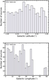 |
Fig. 19 Distributions of radio star candidates as a function of Galactic Latitude (upper panel) and Longitude (lower panel) for the GLOSTAR B-configuration catalog, including the catalog of this work (2° < 𝓁 < 28° 36° < 𝓁 < 40 and 56° < 𝓁 < 60 and |b| < 1°), as listed in Table 3 and the published pilot catalog (28° < 𝓁 < 36° and |b| < 1°) in Table 1 of Dzib et al. (2023). The bin sizes are 0.1° and 2.0° for the upper and lower panel, respectively. The blank region in Galactic longitude 40° < 𝓁 < 56° is not covered by the GLOSTAR survey in B-configuration. |
5.6 Variable sources
Variable radio sources are defined based on the ratios of peak flux densities between the GLOSTAR and CORNISH surveys for compact sources (i.e., Yfactor < 2.0), as outlined in Dzib et al. (2023). A source is considered to be a variable source if (1) it shows a flux density ratio between GLOSTAR and CORNISH larger than 2.0; (2) it is detected in CORNISH at 7σ but is not detected by GLOSTAR at 7σ; (3) it is a GLOSTAR source with a peak flux density higher than the CORNISH detection limit (2.7 mJy beam−1) but is not detected by CORNISH.
Using the criteria listed above, we identified 245 variable radio sources in this work. Together with the 49 variable sources identified in Dzib et al. (2023) for the pilot region, there are a total of 294 variable sources in the GLOSTAR B-configuration catalog. Table 6 lists the source names, peak flux densities, and the suggested source types of all these variable radio sources. The majority of variable sources in the current work (76%=186/245) are found to be extragalactic in origin or infrared quiet based on the classification of this work and CORNISH. The catalog of variable radio sources in this paper includes 12 H II regions, 5 planetary nebulae, and 4 PDRs. The variability of H II regions (e.g., Yang et al. 2022b; Dzib et al. 2023) and planetary nebulae (e.g., Cerrigone et al. 2011; Suárez et al. 2015; Yang et al. 2022b; Dzib et al. 2023) have been reported earlier, which are interesting targets for further exploration.
6 Conclusions
The GLOSTAR survey covers 145 square degrees of the Galactic plane and observes both spectral lines and continuum in the 4–8 GHz using the VLA in B- and D-configurations and the Effelsberg 100-m telescope. In this paper, we present a catalog of continuum sources in the 68 square degrees of the Galactic plane (2° < 𝓁 < 28°, 36° < 𝓁 < 40°, 56° < 𝓁 < 60° and |b| < 1°) observed with the VLA in B-configuration. The images have an angular resolution of 1″, a typical 1σ noise level of ~ 0.08 mJy beam−1, and are restricted to detect extended emission on angular scales smaller than 4″. The high and low reliability catalogs from this region are presented in Tables 3 and B.1, respectively. The main results are summarised below:
We obtained a high-reliability catalog of 5437 sources above 7σ and a low-reliability catalog of 7917 sources with S/N between 5σ and 7σ, using the source extraction tool BLOBCAT. The 1σ noise level of GLOSTAR is spatially varying and 95% of the observing fields have 1σ < 0.13 mJy beam−1. Above the 7σ detection limit, the catalog is typically complete to point sources at 95%. The systematic positional uncertainty of the GLOSTAR B-configuration in this work is ≲0″. 1;
We further investigated the high-reliability catalog (i.e., 5437 sources with S/N ≥ 7σ), with physical properties summarized in Table 5. We extracted the peak intensities from the 9 sub-bands from 4–8 GHz, and determined the inband spectral indices α for 5435 sources by fitting the peak flux density in each sub-band. The uncertainty of the spectral index is negatively correlated with the S/N. The mean value of the in-band spectral index is ~ − 0.6, and 74% of sources have α < −0.1, indicating that the catalog is dominated by non-thermal radio emission. The spectral indices of compact sources between GLOSTAR and THOR are consistent;
We classified all sources above 7 σ-threshold based on the presence or absence of counterparts/emissions in Galactic plane surveys at infrared and submillimeter wavelengths, as well as the SIMBAD database. We identified candidates of 251 H II regions, 784 radio stars, 282 PNe, 4402 extragalactic sources, and 29 others (11 PDRs and 18 unclear). The consistency in classification between GLOSTAR and CORNISH survey is 100% for H II regions and PNe, and 98% for extragalactic sources;
A significant fraction of candidates of the H II region and PNe show a spectral index α < −0.1 (or even α < −0.5), suggesting that there are significant numbers of non-thermal emission sources corresponding to radio jets, winds, and outflows in the vicinity of young H II regions and PNe. As expected, the majority of extragalactic candidates (77%) show α < −0.1, indicating non-thermal emission. The remaining 23% showing α > −0.1 are likely to be the gigahertz peak spectrum sources or high-frequency peakers. For the above three source types, the α < −0.1 group is more likely to be associated with clustered sources compared to the α > −0.1 group;
We compared the measured flux densities between GLOSTAR and other radio surveys (CORNISH, MAGPIS, and THOR), and find a high level of agreement in the flux density and spectral index for compact sources detected in these surveys. We identified 245 variable radio sources listed in Table 6 by comparing the fluxes between the GLOSTAR and CORNISH survey, and most of these variable sources are found to be infrared and submillimeter quiet.
To date, the GLOSTAR survey using VLA in its B-configuration has the highest resolution (~1.0″) and best sensitivity (1σ ~ 0.08 mJy beam−1) for the Galactic plane in the C band (4– 8 GHz). In this work, we present a continuum catalog of 13354 sources ≥ 5σ and 5437 sources ≥ 7σ detection level. From the high-reliability 7σ–threshold catalog, we identified the largest sample of candidates of H II regions, PNe, extragalactic sources, and variable sources in the Galactic plane. It is worth noting that a significant fraction of radio emission associated with massive star formation regions are non-thermal, indicating that relativistic electrons commonly exist. All the catalogs and data are available online at the GLOSTAR website6.
Catalog of 245 variable radio sources identified by this work.
Acknowledgements
We would like to thank the referee David J. Helfand for the helpful comments and suggestions on our manuscript. A.Y.Y. acknowledges support from the National Natural Science Foundation of China (NSFC) grants no. 11988101, no. 11973013, and no. 12303031. S.A.D. acknowledges the M2FINDERS project from the European Research Council (ERC) under the European Union’s Horizon 2020 research and innovation programme (grant no. 101018682). This research was partially funded by the ERC Advanced Investigator Grant GLOSTAR (247078). M.R.R. is a Jansky Fellow of the National Radio Astronomy Observatory, USA. R.D. is a member of the International Max Planck Research School (IMPRS) for Astronomy and Astrophysics at the Universities of Bonn and Cologne. A.Y. would like to thank the help of Philip Lucas and Read Mike when using the data of the UKIDSS survey. The UKIDSS survey was made with the UKIRT Wide Field Camera that was funded by the UK Particle Physics and Astronomy Research Council. This work uses information from the GLOSTAR databases at http://glostar.mpifr-bonn.mpg.de supported by the MPIfR (Max-Planck-Institut für Radioastronomie), Bonn, which is based on observations with the Karl G. Jansky Very Large Array (VLA) of NRAO (The National Radio Astronomy Observatory is a facility of the National Science Foundation operated under cooperative agreement by Associated Universities, Inc.) and 100-m telescope of the MPIfR at Effelsberg. It also made use of information from the ATLASGAL database at http://atlasgal.mpifr-bonn.mpg.de/cgi-bin/ATLASGAL_DATABASE.cgi supported by the MPIfR, Bonn, as well as information from the CORNISH database at http://cornish.leeds.ac.uk/public/index.php which was constructed with support from the Science and Technology Facilities Council of the UK. This work has used data from GLIMPSE and MIPSGAL surveys of the Spitzer Space Telescope, which is operated by the Jet Propulsion Laboratory, California Institute of Technology under a contract with NASA. This publication also makes use of data products from the Wide-field Infrared Survey Explorer, which is a joint project of the University of California, Los Angeles, and the Jet Propulsion Laboratory/California Institute of Technology, funded by the National Aeronautics and Space Administration. This paper used the data products from the Hi-GAL survey of the Herschel telescope which is an ESA space observatory with science instruments provided by European-led Principal Investigator consortia and with important participation from NASA. This research has made use of the SIM-BAD database and the VizieR catalog, operated at CDS, Strasbourg, France. This document was prepared using the collaborative tool Overleaf available at: https://www.overleaf.com/.
Appendix A The pipeline logic flowchart
In this section, we summarize the calibration and imaging steps for the continuum data reduction of the GLOSTAR survey, as discussed in Sect. 2.2 and as outlined in previous papers of GLOSTAR (e.g., Medina et al. 2019; Brunthaler et al. 2021; Dzib ret al. 2023). The logic flowcharts of the calibration and imaging pipeline with the OBIT tasks and processes are shown in Fig. A.1.
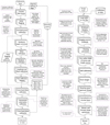 |
Fig. A.1 Flowchart illustration of the GLOSTAR calibration and imaging pipelines. See the text of Sect. 2.2 and Brunthaler et al. (2021) for more details. |
Appendix B The low-reliability catalog
As outlined in Sect. 3, the low-reliability catalog refers to the GLOSTAR sources with a signal-to-noise ratio (S/N) between 5σ and 7σ. We have identified 7917 sources between 5σ and 7σ in this work. Table A.1 lists basic parameters measured from lowreliability sources of the GLOSTAR B-configuration catalog in this work.
The B-configuration catalog of sources with S/N in the range between 5σ to 7σ in this work.
Appendix C The MIR images of H II region candidates
In Fig. C.1, we present three colors images showing the MIR emission from the 251 the H II region candidates identified by this work, based on data from the GLIMPSE survey. Only a small fraction of the MIR images is presented here and the MIR images for the full sample will be available online. Each figure is a 90″ × 90″ centered at the position of the H II region candidate that is shown in blue-white circles, and the three colors are for red, green, and blue for 8.0 µm, 4.5 µm, and 3.6 µm, respectively.
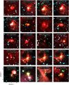 |
Fig. C.1 Three colors images (red=8.0 µm, green=4.5 µm, and blue=3.6 µm) of the H II region candidates identified in this work. Each figure is centered at the position of the identified H II region candidate that is shown in blue-white circles. The images are shown in the boxes with a size of 90″ × 90″. The blue-white pluses refer to the positions of the fragmented H II regions listed in Table 4 or the nearby compact H II regions. The beam size of 1″.0 is shown in the lower-left of each image. Only a small portion of the sample is presented here, and the MIR images for the full sample of 251 H II region candidates are available in electronic form at the Zenodo via https://zenodo.org/uploads/8054107. |
References
- Anderson, L. D., Zavagno, A., Barlow, M. J., García-Lario, P., & NoriegaCrespo, A. 2012, A&A, 537, A1 [NASA ADS] [CrossRef] [EDP Sciences] [Google Scholar]
- Anderson, L. D., Wang, Y., Bihr, S., et al. 2017, A&A, 605, A58 [NASA ADS] [CrossRef] [EDP Sciences] [Google Scholar]
- Anglada, G., Villuendas, E., Estalella, R., et al. 1998, AJ, 116, 2953 [Google Scholar]
- Anglada, G., Rodríguez, L. F., & Carrasco-González, C. 2018, A&ARv, 26, 3 [Google Scholar]
- Beuther, H., Linz, H., Henning, T., et al. 2011, A&A, 531, A26 [NASA ADS] [CrossRef] [EDP Sciences] [Google Scholar]
- Beuther, H., Bihr, S., Rugel, M., et al. 2016, A&A, 595, A32 [NASA ADS] [CrossRef] [EDP Sciences] [Google Scholar]
- Bicknell, G. V., Dopita, M. A., & O’Dea, C. P. O. 1997, ApJ, 485, 112 [NASA ADS] [CrossRef] [Google Scholar]
- Bicknell, G. V., Mukherjee, D., Wagner, A. Y., Sutherland, R. S., & Nesvadba, N. P. H. 2018, MNRAS, 475, 3493 [NASA ADS] [CrossRef] [Google Scholar]
- Bihr, S., Beuther, H., Ott, J., et al. 2015, A&A, 580, A112 [NASA ADS] [CrossRef] [EDP Sciences] [Google Scholar]
- Bihr, S., Johnston, K. G., Beuther, H., et al. 2016, A&A, 588, A97 [NASA ADS] [CrossRef] [EDP Sciences] [Google Scholar]
- Bobrowsky, M., Sahu, K. C., Parthasarathy, M., & García-Lario, P. 1998, Nature, 392, 469 [NASA ADS] [CrossRef] [Google Scholar]
- Brunthaler, A., Menten, K. M., Dzib, S. A., et al. 2021, A&A, 651, A85 [EDP Sciences] [Google Scholar]
- Carey, S. J., Noriega-Crespo, A., Mizuno, D. R., et al. 2009, PASP, 121, 76 [Google Scholar]
- Casassus, S., Nyman, L. Å., Dickinson, C., & Pearson, T. J. 2007, MNRAS, 382, 1607 [NASA ADS] [CrossRef] [Google Scholar]
- Cerrigone, L., Trigilio, C., Umana, G., Buemi, C. S., & Leto, P. 2011, MNRAS, 412, 1137 [NASA ADS] [Google Scholar]
- Cerrigone, L., Umana, G., Trigilio, C., et al. 2017, MNRAS, 468, 3450 [CrossRef] [Google Scholar]
- Chakraborty, A., Roy, N., Wang, Y., et al. 2020, MNRAS, 492, 2236 [Google Scholar]
- Chhetri, R., Ekers, R. D., Kimball, A., et al. 2015, MNRAS, 451, 3228 [NASA ADS] [CrossRef] [Google Scholar]
- Churchwell, E. 2002, ARA&A, 40, 27 [Google Scholar]
- Churchwell, E., Babler, B. L., Meade, M. R., et al. 2009, PASP, 121, 213 [Google Scholar]
- Cohen, M., Chapman, J. M., Deacon, R. M., et al. 2006, MNRAS, 369, 189 [NASA ADS] [CrossRef] [Google Scholar]
- Condon, J. J. 1984, ApJ, 287, 461 [Google Scholar]
- Contreras, Y., Schuller, F., Urquhart, J. S., et al. 2013, A&A, 549, A45 [NASA ADS] [CrossRef] [EDP Sciences] [Google Scholar]
- Cotton, W. D. 2008, PASP, 120, 439 [Google Scholar]
- Csengeri, T., Urquhart, J. S., Schuller, F., et al. 2014, A&A, 565, A75 [NASA ADS] [CrossRef] [EDP Sciences] [Google Scholar]
- Cyganowski, C. J., Whitney, B. A., Holden, E., et al. 2008, AJ, 136, 2391 [Google Scholar]
- Dallacasa, D., Stanghellini, C., Centonza, M., & Fanti, R. 2000, A&A, 363, 887 [NASA ADS] [Google Scholar]
- Dokara, R., Brunthaler, A., Menten, K. M., et al. 2021, A&A, 651, A86 [EDP Sciences] [Google Scholar]
- Dokara, R., Gong, Y., Reich, W., et al. 2023, A&A, 671, A145 [NASA ADS] [CrossRef] [EDP Sciences] [Google Scholar]
- Dzib, S. A., Ortiz-León, G. N., Loinard, L., et al. 2016, ApJ, 826, 201 [CrossRef] [Google Scholar]
- Dzib, S. A., Yang, A. Y., Urquhart, J. S., et al. 2023, A&A, 670, A9 [NASA ADS] [CrossRef] [EDP Sciences] [Google Scholar]
- Feng, H., Wang, J., Li, S., et al. 2021, PASJ, 73, 467 [NASA ADS] [CrossRef] [Google Scholar]
- Fu, Y., Wu, X.-B., Jiang, L., et al. 2022, ApJS, 261, 32 [NASA ADS] [CrossRef] [Google Scholar]
- Gao, X. Y., Reich, P., Hou, L. G., Reich, W., & Han, J. L. 2019, A&A, 623, A105 [NASA ADS] [CrossRef] [EDP Sciences] [Google Scholar]
- Gómez, Y., Rodríguez, L. F., & Garay, G. 2002, ApJ, 571, 901 [CrossRef] [Google Scholar]
- Gómez, J. F., de Gregorio-Monsalvo, I., Lovell, J. E. J., et al. 2005, MNRAS, 364, 738 [CrossRef] [Google Scholar]
- Gong, Y., Ortiz-León, G. N., Rugel, M. R., et al. 2023, A&A, 678, A130 [NASA ADS] [CrossRef] [EDP Sciences] [Google Scholar]
- Greisen, E. W. 2003, in Astrophys. Space Sci. Lib., 285, Information Handling in Astronomy – Historical Vistas, ed. A. Heck, 109 [NASA ADS] [Google Scholar]
- Hales, C. A., Murphy, T., Curran, J. R., et al. 2012, MNRAS, 425, 979 [Google Scholar]
- Hancock, P. J., Murphy, T., Gaensler, B. M., Hopkins, A., & Curran, J. R. 2012, MNRAS, 422, 1812 [Google Scholar]
- Helfand, D. J., Becker, R. H., White, R. L., Fallon, A., & Tuttle, S. 2006, AJ, 131, 2525 [Google Scholar]
- Hoare, M. G., Kurtz, S. E., Lizano, S., Keto, E., & Hofner, P. 2007, Protostars and Planets V (Tucson: University of Arizona Press), 181 [Google Scholar]
- Hoare, M. G., Purcell, C. R., Churchwell, E. B., et al. 2012, PASP, 124, 939 [Google Scholar]
- Hobbs, G., Lyne, A. G., Kramer, M., Martin, C. E., & Jordan, C. 2004, MNRAS, 353, 1311 [NASA ADS] [CrossRef] [Google Scholar]
- Hu, B., Menten, K. M., Wu, Y., et al. 2016, ApJ, 833, 18 [Google Scholar]
- Immer, K., Galván-Madrid, R., König, C., Liu, H. B., & Menten, K. M. 2014, A&A, 572, A63 [NASA ADS] [CrossRef] [EDP Sciences] [Google Scholar]
- Irabor, T., Hoare, M. G., Oudmaijer, R. D., et al. 2018, MNRAS, 480, 2423 [Google Scholar]
- Jankowski, F., Bailes, M., van Straten, W., et al. 2019, MNRAS, 484, 3691 [NASA ADS] [CrossRef] [Google Scholar]
- Kalcheva, I. E., Hoare, M. G., Urquhart, J. S., et al. 2018, A&A, 615, A103 [NASA ADS] [CrossRef] [EDP Sciences] [Google Scholar]
- Kobulnicky, H. A., & Johnson, K. E. 1999, ApJ, 527, 154 [NASA ADS] [CrossRef] [Google Scholar]
- Kurtz, S. 2005, in IAU Symp., 227, Massive Star Birth: A Crossroads of Astrophysics, eds. R. Cesaroni, M. Felli, E. Churchwell, & M. Walmsley, 111 [NASA ADS] [CrossRef] [Google Scholar]
- Liu, H. B., Ho, P. T. P., & Zhang, Q. 2010, ApJ, 725, 2190 [NASA ADS] [CrossRef] [Google Scholar]
- Liu, T., Lacy, J., Li, P. S., et al. 2017, ApJ, 849, 25 [Google Scholar]
- Liu, B., Anderson, L. D., McIntyre, T., et al. 2019, ApJS, 240, 14 [NASA ADS] [CrossRef] [Google Scholar]
- Liu, H.-L., Liu, T., Evans, Neal J., I., et al. 2021, MNRAS, 505, 2801 [NASA ADS] [CrossRef] [Google Scholar]
- Lucas, P. W., Hoare, M. G., Longmore, A., et al. 2008, MNRAS, 391, 136 [Google Scholar]
- Marleau, F. R., Noriega-Crespo, A., Paladini, R., et al. 2008, AJ, 136, 662 [NASA ADS] [CrossRef] [Google Scholar]
- Medina, S. N. X., Urquhart, J. S., Dzib, S. A., et al. 2019, A&A, 627, A175 [NASA ADS] [CrossRef] [EDP Sciences] [Google Scholar]
- Meng, F., Sánchez-Monge, Á., Schilke, P., et al. 2019, A&A, 630, A73 [NASA ADS] [CrossRef] [EDP Sciences] [Google Scholar]
- Molinari, S., Swinyard, B., Bally, J., et al. 2010, PASP, 122, 314 [Google Scholar]
- Murphy, T., Cohen, M., Ekers, R. D., et al. 2010, MNRAS, 405, 1560 [Google Scholar]
- Murray, N., 2011, ApJ, 729, 133 [NASA ADS] [CrossRef] [Google Scholar]
- Nguyen, H., Rugel, M. R., Menten, K. M., et al. 2021, A&A, 651, A88 [NASA ADS] [CrossRef] [EDP Sciences] [Google Scholar]
- Nguyen, H., Rugel, M. R., Murugeshan, C., et al. 2022, A&A, 666, A59 [NASA ADS] [CrossRef] [EDP Sciences] [Google Scholar]
- Ortiz-León, G. N., Menten, K. M., Brunthaler, A., et al. 2021, A&A, 651, A87 [EDP Sciences] [Google Scholar]
- Padovani, M., Marcowith, A., Sánchez-Monge, Á., Meng, F., & Schilke, P. 2019, A&A, 630, A72 [NASA ADS] [CrossRef] [EDP Sciences] [Google Scholar]
- Patel, A. L., Urquhart, J. S., Yang, A. Y., et al. 2023, MNRAS, 524, 4384 [NASA ADS] [CrossRef] [Google Scholar]
- Perley, R. A., & Butler, B. J. 2017, ApJS, 230, 7 [NASA ADS] [CrossRef] [Google Scholar]
- Petrov, L. 2021, AJ, 161, 14 [Google Scholar]
- Purcell, C. R., Hoare, M. G., Cotton, W. D., et al. 2013, ApJS, 205, 1 [Google Scholar]
- Purser, S. J. D., Lumsden, S. L., Hoare, M. G., et al. 2016, MNRAS, 460, 1039 [NASA ADS] [CrossRef] [Google Scholar]
- Qiao, H.-H., Walsh, A. J., Gómez, J. F., et al. 2016, ApJ, 817, 37 [CrossRef] [Google Scholar]
- Qiu, K., Zhang, Q., Beuther, H., & Fallscheer, C. 2012, ApJ, 756, 170 [Google Scholar]
- Qiu, K., Wyrowski, F., Menten, K., Zhang, Q., & Güsten, R. 2019, ApJ, 871, 141 [NASA ADS] [CrossRef] [Google Scholar]
- Rosero, V., Hofner, P., Claussen, M., et al. 2016, ApJS, 227, 25 [Google Scholar]
- Rosero, V., Hofner, P., Kurtz, S., et al. 2019, ApJ, 880, 99 [NASA ADS] [CrossRef] [Google Scholar]
- Schuller, F., Menten, K. M., Contreras, Y., et al. 2009, A&A, 504, 415 [NASA ADS] [CrossRef] [EDP Sciences] [Google Scholar]
- Shao, Y., Wagg, J., Wang, R., et al. 2022, A&A, 659, A159 [NASA ADS] [CrossRef] [EDP Sciences] [Google Scholar]
- Suárez, O., Gómez, J. F., Bendjoya, P., et al. 2015, ApJ, 806, 105 [CrossRef] [Google Scholar]
- Tafoya, D., Gómez, Y., Patel, N. A., et al. 2009, ApJ, 691, 611 [NASA ADS] [CrossRef] [Google Scholar]
- Thompson, M. A., Hatchell, J., Walsh, A. J., MacDonald, G. H., & Millar, T. J. 2006, A&A, 453, 1003 [NASA ADS] [CrossRef] [EDP Sciences] [Google Scholar]
- Thompson, M., Goedhart, S., Goedhart, S., et al. 2016, in MeerKAT Science: On the Pathway to the SKA, 15 [Google Scholar]
- Tian, W. W., Li, Z., Leahy, D. A., & Wang, Q. D. 2007, ApJ, 657, L25 [NASA ADS] [CrossRef] [Google Scholar]
- Tsai, C.-W., Turner, J. L., Beck, S. C., Meier, D. S., & Ho, P. T. P. 2009, AJ, 137, 4655 [CrossRef] [Google Scholar]
- Urquhart, J. S., Thompson, M. A., Moore, T. J. T., et al. 2013, MNRAS, 435, 400 [Google Scholar]
- Urquhart, J. S., Csengeri, T., Wyrowski, F., et al. 2014, A&A, 568, A41 [NASA ADS] [CrossRef] [EDP Sciences] [Google Scholar]
- Urquhart, J. S., König, C., Giannetti, A., et al. 2018, MNRAS, 473, 1059 [Google Scholar]
- Urquhart, J. S., Wells, M. R. A., Pillai, T., et al. 2022, MNRAS, 510, 3389 [NASA ADS] [CrossRef] [Google Scholar]
- van der Tak, F. F. S., & Menten, K. M. 2005, A&A, 437, 947 [NASA ADS] [CrossRef] [EDP Sciences] [Google Scholar]
- Wang, N., Manchester, R. N., Zhang, J., et al. 2001, MNRAS, 328, 855 [NASA ADS] [CrossRef] [Google Scholar]
- Wang, K., Zhang, Q., Wu, Y., Li, H.-b., & Zhang, H. 2012, ApJ, 745, L30 [NASA ADS] [CrossRef] [Google Scholar]
- Wang, Y., Bihr, S., Rugel, M., et al. 2018, A&A, 619, A124 [NASA ADS] [CrossRef] [EDP Sciences] [Google Scholar]
- Wang, P. F., Han, J. L., Han, L., et al. 2020, A&A, 644, A73 [NASA ADS] [CrossRef] [EDP Sciences] [Google Scholar]
- Wang, Y., Qiu, K., Cao, Y., et al. 2022, ApJ, 927, 185 [NASA ADS] [CrossRef] [Google Scholar]
- Wenger, M., Ochsenbein, F., Egret, D., et al. 2000, A&AS, 143, 9 [NASA ADS] [CrossRef] [EDP Sciences] [Google Scholar]
- White, R. L., Becker, R. H., Helfand, D. J., & Gregg, M. D. 1997, ApJ, 475, 479 [Google Scholar]
- White, R. L., Becker, R. H., & Helfand, D. J. 2005, AJ, 130, 586 [NASA ADS] [CrossRef] [Google Scholar]
- Wilner, D. J., Reid, M. J., & Menten, K. M. 1999, ApJ, 513, 775 [NASA ADS] [CrossRef] [Google Scholar]
- Wright, E. L., Eisenhardt, P. R. M., Mainzer, A. K., et al. 2010, AJ, 140, 1868 [Google Scholar]
- Wyrowski, F., Güsten, R., Menten, K. M., et al. 2016, A&A, 585, A149 [NASA ADS] [CrossRef] [EDP Sciences] [Google Scholar]
- Yang, A. Y., Thompson, M. A., Urquhart, J. S., & Tian, W. W. 2018, ApJS, 235, 3 [Google Scholar]
- Yang, A. Y., Thompson, M. A., Tian, W. W., et al. 2019, MNRAS, 482, 2681 [NASA ADS] [CrossRef] [Google Scholar]
- Yang, A. Y., Urquhart, J. S., Thompson, M. A., et al. 2021, A&A, 645, A110 [EDP Sciences] [Google Scholar]
- Yang, A. Y., Urquhart, J. S., Wyrowski, F., et al. 2022a, A&A, 658, A160 [NASA ADS] [CrossRef] [EDP Sciences] [Google Scholar]
- Yang, J., Chen, Y., Gurvits, L. I., et al. 2022b, MNRAS, 511, 280 [NASA ADS] [CrossRef] [Google Scholar]
- Yao, J. M., Manchester, R. N., & Wang, N. 2017, ApJ, 835, 29 [NASA ADS] [CrossRef] [Google Scholar]
- Zhang, Y., & Kwok, S. 2009, ApJ, 706, 252 [CrossRef] [Google Scholar]
In Appendix C, we present the MIR emission around the H II region candidates.
All Tables
Summary of VLA continuum observations in B-configuration for the region (2° < ℓ < 28°, 36° < ℓ < 40°, and 56° < ℓ < 60°) of the GLOSTAR survey.
GLOSTAR B-configuration catalog for 2° < ℓ < 28°, 36° < ℓ < 40 and 56° < ℓ < 60° and |b| < 1°.
GLOSTAR D-configuration sources that are detected as fragmented sources (e.g., multiple components or over-resolved of an extended source) in the B-configuration images.
The B-configuration catalog of sources with S/N in the range between 5σ to 7σ in this work.
All Figures
|
Fig. 1 RMS noise map of the 2° < ℓ < 40°, 56° < ℓ < 60°, and |b| < 1° region observed in B-configuration of the GLOSTAR survey. Each field is made by sampling on a size of 3′.25. High noise levels are found in the fields associated with bright emissions (the star-forming regions, H II regions, and other bright radio-emitting sources), observed at low declinations (close to the Galactic center), observed in bad weather conditions, and located at the edge area of the survey. High noise striping in Galactic Latitude is due to changes in observing conditions between scans. For B-configuration data of the “pilot region” of the GLOSTAR survey (28° < ℓ < 36°, |b| < 1°), see Dzib et al. (2023). |
| In the text | |
|
Fig. 2 Distributions of RMS noise level of the GLOSTAR B-configuration images (Fig. 1). The bin width is 0.002 mly beam−1. The red, blue and black histograms represent values determined for the region discussed here (2° < ℓ < 28°, 36° < ℓ < 40°, and 56° < ℓ < 60°), the pilot region (28° < ℓ < 36°) published in Dzib et al. (2023), and the combined area 2° < ℓ < 40°, 56° < ℓ < 60° area. The median RMS noise level is ~ 0.08 mJy beam−1 and 95% of the fields have a noise level < 0.13 mJy beam−1. |
| In the text | |
|
Fig. 3 Comparison of GLOSTAR astrometry with CORNISH and VLBI results. Top panel: offsets between GLOSTAR B-configuration positions (this work) and the positions of VLBI calibrators (black crosses, red filled ellipse) for 44 counterparts, and the offsets between CORNISH and VLBI calibrators for 75 counterparts (blue crosses, green filled ellipse). The VLBI calibrators have a (sub)milliarcsec positional accuracy (Petrov 2021). The median and standard deviation of the offsets are −0″.06 and −0″.11, suggesting a systematic positional difference of ≲0″.1 for the GLOSTAR and Very Long Baseline Array (VLBA) calibrators. Bottom panel: position offsets between the GLOSTAR B-configuration and CORNISH positions for 669 counterparts. The mean and standard deviation of the offsets are 0″.08 and 0″.16, suggesting a systematic positional difference of ≲0″.1 for the GLOSTAR and CORNISH. |
| In the text | |
|
Fig. 4 Cumulative distribution of spurious sources (black histogram) and all detections (blue histogram) as a function of the S/N (1σ ~ 0.08 mJy), to estimate the spurious sources expected in the GLOSTAR survey. The red dashed line fitted to the negative detections indicates the expected spurious sources. Below 4.5 σ, the detections are dominated by spurious sources (occupying 93%) and the false detections decrease to 186 at 6.1 σ. Above 7 σ, fewer than 5 sources are expected to be false. |
| In the text | |
|
Fig. 5 Completeness fraction of recovered artificial sources as a function of the peak flux density of the total added artificial sources. The completeness of the selected fields with different typical noises are shown in different colors. The mean RMS values for the high, low, and typical noise regions are 0.12 mJy beam−1, 0.06 mJy beam−1, and 0.08 mJy beam−1, respectively. 95% completeness limit is reached at a flux density of ~0.35 mJy for the best case G22.5 (red line) and ~0.8 mJy for the worst case G06.5. Typically, the GLOSTAR survey in B-configuration is 95% complete to point sources at the ~0.6 mJy level (i.e., the chosen 7 σ threshold for the catalog in Sect. 3.3), as shown in black line for all the selected fields. See the completeness in Sect. 3.4 for details. |
| In the text | |
|
Fig. 6 Example of the peak flux as a function of the in-band frequency for bright sources (top panel) and faint sources (bottom panel). Each data point (circle or triangle) refers to the peak intensity at each sub-band, with the error of the peak measurement. The solid and dashed lines in the top panel show the best fit to the peak flux densities from 9 sub-bands for two bright sources: G020.0808−00.1354 (α = 1.1 ± 0.07) and G021.7700+00.8423 (α = −0.92 ± 0.04), respectively. The solid and dashed lines in the bottom panel present the spectral fitting of 5 and 6 sub-bands for two faint sources: GOll.9357+00.2871 (α = −1.7 ± 0.36) and G036.8880+01.0288 (α = 2.5 ± 0.6), respectively. |
| In the text | |
|
Fig. 7 Flowchart illustration of the radio source classification process. See the text of Sect. 3.6 for further details. |
| In the text | |
|
Fig. 8 Illustration of source types in the classification process of Sect. 3.6. From top to bottom: typical multiband images of a radio source classified as an H II region, a planetary nebula, a radio star and a extragalactic source. From left to right: three-colors composition image of UKIDSS (red = 2.2 µm, green = 1.65 µm, blue = 1.2 µm), three-color composition image of GLIMPSE (red = 8 µm, green = 4.5 µm, blue = 3.6 µm), three-color composition of WISE (red = 22 µm, green = 12 µm, blue = 4.6 µm), MIPSGAL 24 µm, Hi-GAL 70 µm, Hi-GAL 160 µm, Hi-GAL 250 µm, Hi-GAL 500 µm, and ATLASGAL 870 µm. The blue and white circle in the center show the position of radio emission. The FWHM beams of UKIDSS (0.8″), GLIMPSE (2″), WISE (6″ at 12 µm), MIPSGAL (6″ at 24 µm), Hi-GAL (6″–35″), ATLASGAL (19″) are indicated by the white circles with black hatched lines shown in the lower-left corner of each image. |
| In the text | |
|
Fig. 9 Example of cluster sources in three cases. Top panel: the cluster sources in normal case. Middle-panel: example of clusters consists of over-resolved sources are listed in Table 4. Bottom panel: example of clusters with semi-ring-like fragments. In this case, the sources with semi-ring-like structures have been removed from the catalog. The positions of 7σ cluster sources are noted by blue and white pluses. The Galactic name of each figure refers to the source in the center position. The cyan contours are emission from B-configuration images (this work), starting at 5σ with 5σ increment. The background of each image presents the B+D configuration of GLOSTAR (Brunthaler et al. 2021). The FWHM beams of B (1″.0) and B+D configuration (4″.0) are presented by the white circles in the lower-right and lower-left corners of each image. |
| In the text | |
|
Fig. 10 Distribution of 6894 GLOSTAR B-configuration 7 σ–threshold sources as a function of Galactic Latitude (upper panel) and Longitude (lower panel) for the B-configuration catalog, including the catalog of this work (2° < ℓ < 28° 36° < ℓ < 40 and 56° < ℓ < 60 and |b| < 1°), as listed in Table 3 and the published pilot catalog (28° < ℓ < 36° and |b| < 1°) in Dzib etal. (2023). The bin sizes are 0.1° and 2.0° for the upper and lower panel, respectively. The blank region in Galactic longitude 40° < ℓ < 56° is not covered by the GLOSTAR survey in B-configuration. |
| In the text | |
|
Fig. 11 Distribution of source effective radius for the 6894 sources in the 7 σ–threshold catalog of this work (Table 3) and the published pilot catalog in Dzib et al. (2023). |
| In the text | |
|
Fig. 12 Distributions of peak (upper panel) and integrated (lower panel) flux density for the 6894 7 σ − threshold sources of GLOSTAR B-configuration, including Table 3 and the published pilot catalog in Dzib et al. (2023). |
| In the text | |
|
Fig. 13 Distribution of spectral index α for the 7 σ −threshold catalog of the GLOSTAR B-configuration, including Table 3 and the published pilot catalog in Dzib et al. (2023). |
| In the text | |
|
Fig. 14 Comparison of flux densities between GLOSTAR and CORNISH. Top panel: the comparison of flux densities for 669 compact sources detected by both CORNISH and GLOSTAR catalogs. The error bar of each point shows the uncertainty of flux. Bottom panel: the histogram of the flux density ratios of compact sources between CORNISH and GLOSTAR. The black line displays the Gaussian fit to the histogram. The dashed line presents the mean value of the distribution, with mean and standard deviation of the flux ratio from the Gaussian fit are 1.14 and 0.3, respectively. |
| In the text | |
|
Fig. 15 Comparison of flux densities between GLOSTAR and MAGPIS. Top panel: The comparison of measured flux densities for 663 MAGPIS compact sources at 5 GHz (White et al. 2005) common to GLOSTAR. These compact sources are defined as sources with angular sizes < 6″ in MAGPIS. The dashed line means the flux densities are the same in MAGPIS and GLOSTAR. At the top, we show the color bar for the Yfactor (defined as Sint/Speak) of the GLOSTAR detections, indicating the emission of sources in the GLOSTAR image are unresolved (defined as Yfactor < 1.1 in Sect. 4.3.1), compact (1.1 < Yfactor < 2.0) or extended (Yfactor > 2.0). Bottom panel: The comparison of flux densities of 484 compact MAGPIS at 1.4 GHz that are also detected by GLOSTAR at 5 GHz. The 1.4 flux densities from GLOSTAR is extrapolated from the 5 GHz flux densities and spectral indices of the GLOSTAR catalog. |
| In the text | |
|
Fig. 16 Distribution for the difference (αBconf − αTHOR) in the measured spectral indices for 1390 compact THOR sources common to GLOSTAR in B-configuration. The black solid line means the Gaussian fit for the distribution, giving a mean value of −0.04 ± 0.03 (the error of the mean is from the Gaussian fit) and a standard deviation of 0.78. |
| In the text | |
|
Fig. 17 Distributions of spectral index and peak flux densities of HII region candidates in GLOSTAR B-configuration. Top panel: the histogram of the measured spectral index for the total 390 H II region candidates of GLOSTAR B-configuration. The hatched histogram represents the 183 candidates with σα < 0.2. The bin size is 0.25. The 183 candidates are divided into two subsamples: (1) 120 H II regions with α and (2) 63 H II regions with α > −0.1, indicating non-thermal and thermal emissions, respectively. Bottom panel: the cumulative distribution of the peak flux densities for the α < −0.1 sample (orange line) and the α > −0.1 sample (black line). The orange and black vertical dashed lines show the mean values of 9.5 mJy beam−1 and 31.6 mJy beam−1 for the two subsamples, respectively. |
| In the text | |
|
Fig. 18 Example of two H II region candidates with positive and negative in-band spectral index, as discussed in Sect. 5.2. The top two rows show the 8 sub-bands of the GLOSTAR image. The bottom-left panel shows the averaged image at 5.8 GHz used to extract the source, and the bottom-right panel shows the in-band spectral index fitting for the two compact H II regions candidates: the solid line for G024.7897 (Yfactor = 1.02) with α = 1.43 ± 0.02 and the dashed line for G024.7888 (Yfactor = 1.97) with α = −0.55 ± 0.04. The FWHM beam of GLOSTAR in B-configuration (1.0″) is indicated by the white circles in the lower-left corner of each image. There is a clear trend that the fluxes increase and decrease as the increasing frequencies in the sub-bands for G024.7897 and G024.7888 respectively. |
| In the text | |
|
Fig. 19 Distributions of radio star candidates as a function of Galactic Latitude (upper panel) and Longitude (lower panel) for the GLOSTAR B-configuration catalog, including the catalog of this work (2° < 𝓁 < 28° 36° < 𝓁 < 40 and 56° < 𝓁 < 60 and |b| < 1°), as listed in Table 3 and the published pilot catalog (28° < 𝓁 < 36° and |b| < 1°) in Table 1 of Dzib et al. (2023). The bin sizes are 0.1° and 2.0° for the upper and lower panel, respectively. The blank region in Galactic longitude 40° < 𝓁 < 56° is not covered by the GLOSTAR survey in B-configuration. |
| In the text | |
|
Fig. A.1 Flowchart illustration of the GLOSTAR calibration and imaging pipelines. See the text of Sect. 2.2 and Brunthaler et al. (2021) for more details. |
| In the text | |
|
Fig. C.1 Three colors images (red=8.0 µm, green=4.5 µm, and blue=3.6 µm) of the H II region candidates identified in this work. Each figure is centered at the position of the identified H II region candidate that is shown in blue-white circles. The images are shown in the boxes with a size of 90″ × 90″. The blue-white pluses refer to the positions of the fragmented H II regions listed in Table 4 or the nearby compact H II regions. The beam size of 1″.0 is shown in the lower-left of each image. Only a small portion of the sample is presented here, and the MIR images for the full sample of 251 H II region candidates are available in electronic form at the Zenodo via https://zenodo.org/uploads/8054107. |
| In the text | |
Current usage metrics show cumulative count of Article Views (full-text article views including HTML views, PDF and ePub downloads, according to the available data) and Abstracts Views on Vision4Press platform.
Data correspond to usage on the plateform after 2015. The current usage metrics is available 48-96 hours after online publication and is updated daily on week days.
Initial download of the metrics may take a while.