| Issue |
A&A
Volume 674, June 2023
Gaia Data Release 3
|
|
|---|---|---|
| Article Number | A25 | |
| Number of page(s) | 52 | |
| Section | Catalogs and data | |
| DOI | https://doi.org/10.1051/0004-6361/202245353 | |
| Published online | 16 June 2023 | |
Gaia Data Release 3
Gaia scan-angle-dependent signals and spurious periods⋆
1
Department of Astronomy, University of Geneva, Chemin Pegasi 51, 1290 Versoix, Switzerland
2
Department of Astronomy, University of Geneva, Chemin d’Ecogia 16, 1290 Versoix, Switzerland
3
Institut d’Estudis Espacials de Catalunya (IEEC), c. Gran Capità, 2-4, 08034 Barcelona, Spain
4
Institut de Ciències del Cosmos (ICCUB), Universitat de Barcelona (UB), c. Martí i Franquès, 1, 08028 Barcelona, Spain
5
Lund Observatory, Department of Astronomy and Theoretical Physics, Lund University, Box 43 22100 Lund, Sweden
6
GEPI, Observatoire de Paris, Université PSL, CNRS, 5 Place Jules Janssen, 92190 Meudon, France
7
Laboratoire d’Astrophysique de Bordeaux, Univ. Bordeaux, CNRS, B18N, Allée Geoffroy Saint-Hilaire, 33615 Pessac, France
8
Institute of Astronomy, University of Cambridge, Madingley Road, Cambridge CB3 0HA, UK
9
Kavli Institute for Cosmology, Institute of Astronomy, Madingley Road, Cambridge CB3 0HA, UK
10
INAF – Osservatorio Astrofisico di Torino, Via Osservatorio 20, 10025 Pino Torinese, Italy
11
Institut d’Astrophysique et de Géophysique, Université de Liège, 19c, Allée du 6 Août, 4000 Liège, Belgium
12
F.R.S.-FNRS, Rue d’Egmont 5, 1000 Brussels, Belgium
13
RHEA for European Space Agency (ESA), Camino Bajo del Castillo, s/n, Urbanizacion Villafranca del Castillo, Villanueva de la Cañada, 28692 Madrid, Spain
14
Sednai Sàrl, 4 Rue des Marbiers, 1204 Geneva, Switzerland
15
European Space Agency (ESA), European Space Astronomy Centre (ESAC), Camino Bajo del Castillo, s/n, Urbanizacion Villafranca del Castillo, Villanueva de la Cañada, 28692 Madrid, Spain
16
Institut d’Astronomie et d’Astrophysique, Université Libre de Bruxelles CP 226, Boulevard du Triomphe, 1050 Brussels, Belgium
Received:
2
November
2022
Accepted:
13
March
2023
Abstract
Context. Gaia Data Release 3 (Gaia DR3) time series data may contain spurious signals related to the time-dependent scan angle.
Aims. We aim to explain the origin of scan-angle-dependent signals and how they can lead to spurious periods, provide statistics to identify them in the data, and suggest how to deal with them in Gaia DR3 data and in future releases.
Methods. Using real Gaia (DR3) data alongside numerical and analytical models, we visualise and explain the features observed in the data.
Results. We demonstrated with Gaia (DR3) data that source structure (multiplicity or extendedness) or pollution from close-by bright objects can cause biases in the image parameter determination from which photometric, astrometric, and (indirectly) radial velocity time series are derived. These biases are a function of the time-dependent scan direction of the instrument and thus can introduce scan-angle-dependent signals, which due to the scanning-law-induced sampling of Gaia can result in specific spurious periodic signals. Numerical simulations in which a period search is performed on Gaia time series with a scan-angle-dependent signal qualitatively reproduce the general structure observed in the spurious period distribution of photometry and astrometry, and the associated spatial distributions on the sky. A variety of statistics allows for the deeper understanding and identification of affected sources.
Conclusions. The origin of the scan-angle-dependent signals and subsequent spurious periods is well understood and is mostly caused by fixed-orientation optical pairs with a separation < 0.5″ (including binaries with P ≫ 5 y) and (cores of) distant galaxies. Although most of the sources with affected derived parameters have been filtered out from the Gaia archive nss_two_body_orbit and several vari-tables, Gaia DR3 data remain that should be treated with care (no sources were filtered from gaia_source). Finally, the various statistics discussed in the paper can be used to identify and filter affected sources and also reveal new information about them that is not available through other means, especially in terms of binarity on sub-arcsecond scale.
Key words: methods: data analysis / techniques: photometric / methods: numerical / techniques: radial velocities / astrometry
Table A.1 is also available at the CDS via anonymous ftp to cdsarc.cds.unistra.fr (130.79.128.5) or via https://cdsarc.cds.unistra.fr/viz-bin/cat/J/A+A/674/A25 and at the Gaia archive via https://gea.esac.esa.int/archive/
Corresponding author: B. Holl, e-mail: mailto: This email address is being protected from spambots. You need JavaScript enabled to view it. .
Deceased.
© The Authors 2023
 Open Access article, published by EDP Sciences, under the terms of the Creative Commons Attribution License (https://creativecommons.org/licenses/by/4.0), which permits unrestricted use, distribution, and reproduction in any medium, provided the original work is properly cited.
This article is published in open access under the Subscribe to Open model. This email address is being protected from spambots. You need JavaScript enabled to view it. to support open access publication.
1. Introduction
The ongoing processing and analyses of Gaia data by the data processing analysis consortium (DPAC) and scientific community is leading to an increasingly more detailed and refined understanding of the instrument responses and of the data properties. This paper is mainly dedicated to so-called scan-angle-dependent signals in the Gaia data, which is a product of the on-sky source structure (mainly multiplicity or extendedness), Gaia scanning law, the on-board sampling and windowing observation strategy, and on-ground observation modelling. These signals can lead to the emergence of biases in the derived parameters such as the periodicity, giving rise to specific spurious periods.
A quick overview of the paper is given in the discussion in Sect. 7, where the whole paper is condensed around several relevant topics and questions that point out the relevant sections for further reading.
To properly understand and explain the mentioned effects, we structured the paper in the following way. First, the basic Gaia observation mode and its properties are explained in Sect. 2. Then Sect. 3 discusses and demonstrates the relevant scan-angle-related modelling errors for each Gaia instrument that can be introduced in the derived data. Examples and interpretation of observed spurious period distributions are then discussed in Sect. 4. In Sect. 5 we introduce a photometric and astrometric scan-angle-dependent bias signal model and demonstrate through simulations how it qualitatively reproduces the observed spurious periods. Section 6 then focuses on statistics that can detect scan-angle-dependent signals and several other relevant features. Section 7 contains condensed discussions around the subjects related to this paper, which is followed by our concluding remarks in Sect. 8.
In Appendix A we describe the Gaia archive table data that are published with this paper for all sources with published time series in Gaia Data Release 3 (Gaia DR3), containing the statistical parameters of Sect. 6. Appendix B contains additional examples of sources that are affected by the scan-angle signal. In Appendix C we show the sky distribution of specific spurious peaks as identified in Sect. 5.4. Finally, Appendix D describes the conversion between equatorial and ecliptic scan position angles.
2. How Gaia observes the sky
We start with a brief overview of the Gaia scanning-law properties that are relevant for this study (for more details, see Gaia Collaboration 2016; Lindegren & Bastian 2010; de Bruijne et al. 2010). We only consider operations under the nominal scanning law (NSL) and ignored other non-nominal modes because they do not affect the majority of the data significantly and are not essential for the understanding of the discussed features. The NSL dictates the way in which the Gaia spacecraft scans the sky; its two fields of view are separated by 106.5°, and it rotates in a plane orthogonal to the spacecraft spin axis with a period of 6 h. Each field of view has an instantaneous coverage of about 0.5 deg2 (0.72° ×0.69°), and a source is typically observed sequentially by at least one pair of the preceding and following field of view, with decreasing frequency of longer sequences of recurring observations due to the slow and non-constant precession rate of the spin axis (see for example Eyer et al. 2017, for these all-sky sequence statistics). For observations around a certain time at a specific sky location, a low or high AC-scan velocity (see Sect. 2.3) will produce more or fewer sequences of recurring observations, respectively. If the spin axis had a fixed orientation in space, a single great circle alone would be scanned on the sky. In reality, the spacecraft orbits the second Lagrangian point (L2) of the Earth-Sun system, and thus, the spacecraft has to rotate its spin axis with a yearly cycle to keep the instrumentation behind the solar shield. To be able to acquire useful astrometric measurements throughout the sky (in terms of temporal sampling and required instrument orientation), the spin axis is made to precess at a 45° angle around the direction towards the Sun with a frequency of 5.8 cycles yr−1, which is about 63.0 d per cycle (see the left panel of Fig. 1). To be precise, this precession is around a fictitious nominal Sun direction as seen from L2 (that is, along the Earth-Sun vector), and not from Gaia orbiting L2, although the offset is always less than 0.15° (see Gaia Collaboration 2016). This gives rise to the specific observation distribution, as illustrated in the top panel of Fig. 2, along with the published Gaia DR3 source sky density in the bottom panel for comparison.
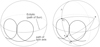 |
Fig. 1. Overview of the Gaia scanning law. Left: during the nominal scanning law, the spin axis z makes overlapping loops around the Sun at a separation of 45° and rate of 5.8 cycles yr−1. Right: one source at point a may be scanned whenever z is 90° from a, that is, on the great circle A at z1, z2, z3, etc. Reproduction with permission of Fig. 7 in Gaia Collaboration (2016). |
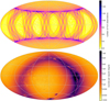 |
Fig. 2. Ecliptic coordinate plots with longitude zero at the centre and increasing to the left. Top panel: simulated number of field-of-view observations during the nominal scanning law phase of the Gaia DR3 time range. Bottom panel: sky density of the published Gaia DR3 sources. |
Because of the approximately 3:1 aspect ratio of the Gaia primary mirrors (Gaia Collaboration 2016) and matching 1:3 pixel aspect ratio (to achieve diffraction-limited sampling), the highest image sampling resolution of 58.9 mas/pixel is achieved in the so-called along-scan (AL) direction. This is the direction in which a field of view passes over a particular source due to the spinning motion of the spacecraft. Its direction is indicated by the time-dependent scan angle ψ that is illustrated in Fig. 6. The direction orthogonal to AL is called across-scan (AC), and it is sampled with a resolution of 176.8 mas/pixel. Depending on the magnitude of a detected source and the instrument, the details of the data acquisition vary, as described in Sect. 3.
The most important information in this section is that the vast majority of Gaia information is encoded and contained in the AL-scan measurement, which is taken in the direction of the scan angle over a source at a particular time.
2.1. Scan-angle distribution of source observations
The nominal scanning law not only dictates the cadence and thus total number of observations for each position on the sky (as shown in the top panel of Fig. 2), but also the associated observation scan angles. The scan angle ψ in Fig. 6 at a certain sky position and time is zero when pointing toward the local equatorial north and 90° when pointing towards the local equatorial east direction. To illustrate the all-sky scan-angle distribution in the bottom panel of Fig. 3, we collapsed all sky positions along the ecliptic longitude because the nominal scanning law induces the most distinctive scan-angle variations as a function of ecliptic latitude, as also seen in the observation counts of Fig. 3. We use the hierarchical equal area isolatitude pixelation (HEALPix) of the celestial sphere (Górski et al. 2002). The normal (equatorial-based) scan-angle would cause a sky-position-dependent offset of the scan-angles of a source due to the offset between the equatorial and ecliptic reference frame, however, thus blurring the image. To circumvent this issue, we thus introduce the ecliptic scan angle, ψecl, which is defined with respect to the ecliptic local north and east directions. It effectively is the (equatorial) scan angle plus an offset that depends on sky position, as given by Eq. (D.7).
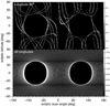 |
Fig. 3. Ecliptic scan-angle distribution for the nominal scanning law during the Gaia DR3 time range. For a certain ecliptic latitude (horizontal slice), the colour represents the occupancy percentage per 1° scan-angle bin (summing up to 100% over all scan angles) to highlight non-uniformities in the scan-angle distribution at different ecliptic latitudes. Top panel: distribution for sources along a half-circle slice at ecliptic longitude λ = 90°. Bottom panel: same as top panel, but for an all-sky uniform HEALPix grid of sources (that is, all ecliptic longitudes for a given latitude). The strong imbalance of scan angles for sources |β|≤45° has a strong impact on the propagation strength of certain scan-angle-dependent signals; see text for details. |
The top panel of Fig. 3 shows the ecliptic scan-angle distribution for sources along a half-circle slice with ecliptic longitude λ = 90°, starting at the north ecliptic pole (NEP; at ecliptic latitude β = 90°) and extending to the south ecliptic pole (SEP, at β = −90°). The specific choice of λ = 90° was made because it intersects the equatorial north pole, causing the equatorial and ecliptic scan angles to be identical for β < 66.6° and 180° offset above. We normalised the distribution of observation scan-angles over each ecliptic latitude bin with per-source normalised observation weights to compensate for the different numbers of observations of each source position. Then we colour-coded this to highlight non-uniformities in the distribution of scan angles of sources at different ecliptic latitudes: yellow means a high concentration of scan angles at the particular scan-angle bin (bin width 1°), and dark red means that it was only sampled once or twice.
Although the distribution is approximately spread out evenly towards the ecliptic poles, it becomes much tighter and imbalanced for |β|≤45°. These asymmetries become even more apparent when we combine the scan-angle distribution of sources that are uniformly distributed over the sky on a HEALPix grid level 5, as shown in the bottom panel of Fig. 3. The sources close to the ecliptic poles have indeed very similarly regularly spread scan angles (red). The feature resulting from the geometric constraints of the NSL is now very clear: a circle of avoidance for |β|< 45° centred on (ψecl, β) = (−90° ,0° ) and (90° ,0° ), with an overabundance of observations at the very specific scan angles close to the border of these circles (yellow). Additionally, for sources located at |β|∼45°, the scan angles are very clustered at ecliptic scan angles ψecl = ±90° (upper and lower parts of the yellow circles) with hardly any observations at other scan angles, that is, the dark horizontal zones. The very specific clusters in scan angle for sources with |β|≤45° have important implications for the selection function of signals that have a strong dependence on scan angle, such as astrometric orbits and the scan-angle-dependent signals we discuss here: depending on the phasing of this signal, it might or might not be detectable. For example, a signal that peaks in the circle of avoidance might be completely undetected.
Continuing with the properties of the nominal scanning law, we noted earlier that the spacecraft rotation around the Sun will induce a yearly rotation of its spin axis. In Fig. 4 we show the temporal distribution of the scan angles of five positions along the ecliptic half-circle used in the top panel of Fig. 3. The figure shows that this yearly rotation clearly dominates the temporal distribution of the scan angles of the sources. To guide the eye, we added the slope of this yearly cyclic rotation with a blue line. Depending on the ecliptic hemisphere, this gives a negative or positive slope.
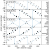 |
Fig. 4. Time series of the ecliptic scan-angle distribution during the Gaia DR3 NSL time range for five ecliptic latitudes along the half-circle slice with ecliptic longitude λ = 90° (same as the top panel of Fig. 3). Each point is semi-transparent, so that a darker colour means more observations. Blue cyclic lines illustrate the slopes due to the yearly rotation around the Sun. The histogram on the right side has a bin size of 32.7° (360/11) and shows the relative distribution of scan angles, corresponding to the top panel of Fig. 3 for the specified ecliptic latitudes. |
In addition to the yearly rotation, we have additional modulations due to the spin axis rotation around the nominal Sun direction, as is illustrated in the right panel of Fig. 1 for a source at an arbitrary position a. For simplicity, we study a source located at the north ecliptic pole (β = 90° ) in more detail, that is, the top panel of Fig. 4. In this case, all observations are generated when the spin axis crosses the ecliptic equator, which occurs at a rate of about twice the spin-axis precession rate, that is, 11.6 cycles yr−1, or approximately 31.5 d intervals. Alternating with these crossings are upwards/ahead or downwards/trailing the Sun nominal direction, which are therefore offset vertically, as is clearly visible in the distribution of data points in Fig. 4. However, to be precise, the precession rate is not constant during its 63 d period, nor during a one-year cycle (see Eq. (1) of Gaia Collaboration 2016), thus the interval between up- and downward cycles is not as symmetric as we suggested just now. This already indicates one of the reasons for the complexity and broadness of the spurious period peak distributions discussed later in Sects. 4 and 5.
The NSL scanning law observations in this section were generated by a reduced version of the astrometric global iterative solution, AGISLab (Holl et al. 2012), but the same data can be generated with the public Gaia observation forecast tool (GOST)1.
2.2. Angular coverage of extended sources
Extended objects are directly concerned by the dependence of the NSL on the ecliptic latitude. For these objects with a spatial extension, the variety of scan angles is crucial for reconstructing their structures. We define the angular coverage as the fraction of the sky area that is covered by the union of the observation windows for a particular source, relative to the ideal case of a uniform distribution in scan angles (see Fig. 3 in Ducourant et al. 2023, for an illustration, and Garcez de Oliveira Krone Martins 2011). This quantity is mainly dependent on how the scan angles are spread over the source. Preferential scan directions will result in lower angular coverage. Figure 5 presents the distribution of ∼1.3 million extragalactic sources on the sky in ecliptic coordinates, colour-coded with their angular coverage. The surface coverage of sources with |β|< 30° is frequently lower than 85%, as is well understood from the circle of avoidance in scan angles shown in Fig. 3. Only for sources with a coverage larger than 85% is the morphology of extended sources provided in Gaia DR3 data.
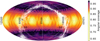 |
Fig. 5. Sky distribution in ecliptic coordinates of extragalactic sources analysed in terms of surface brightness profile in Gaia DR3, colour-coded with the angular coverage of the sources. The non-linear shader table reveals the NSL pattern. |
2.3. Across-scan velocity and scan phase
As mentioned in Sect. 2, there are variations in the AC velocity of sources transiting the focal plane. The AC-scan velocity varies sinusoidally with time, with the nominal satellite rotation period of 6 h and an amplitude of 173 mas s−1 (Gaia Collaboration 2016). This means that the AC-scan velocity varies along the great circle that is scanned on the sky by each field of view (FoV) over this 6 h rotation. The phase of this oscillation is determined by the scan phase (not to be confused with the previously discussed scan angle), which is defined as the angle between the plane containing the Sun and the spin axis and the plane spanned by the spin axis and the vector pointing exactly in between the two fields of view; see Sect. 5.2 of Gaia Collaboration (2016) and Fig. 2 of Lindegren et al. (2012) for details about the scan phase and its definition, and Sect. 3.1 for a calibration related effect. The reference point of this scan phase slowly drifts over time due to the 63 d precession of the spin axis. For several-day stretches of time, this means that for particularly narrow localised regions on the sky, the AC-scan velocity will vary slowly. When it is close to zero, it means that the succeeding great-circle passes will be able to scan this position more times, while a high AC-scan velocity will cause the source to drift out of the FoV before many passes can be made. At the time of the sinusoidal crossing of zero AC-scan velocity, some sky positions along the great circle experience a reverse of the AC-scan velocity in a period of a few days, causing them to stay within the across-scan bounds of the transiting FoVs. At some specific moments, this can cause the accumulation of very many (near-) continuous transits along a small band on the sky called a cusp, for example, 28 FoVs during ∼3.5 d. These cusps usually occur in regions on the sky with |β|≤45°.
3. Scan-angle-dependent instrument calibration features
The several instruments on board Gaia each have their own specific way of collecting data, which are processed differently to extract the most relevant science data (see Gaia Collaboration 2016 for a general overview and the references below for full details). In this section, we concentrate on the aspects of the data collection for each instrument and on the processing that is relevant to the introduction of spurious signals that are dependent on the scan angle.
Examining each instrument separately, we start with the astrometric field in Sect. 3.1, followed by the blue and red photometer instrument in Sect. 3.2, followed in turn by the radial velocity spectrometer instrument in Sect. 3.3.
3.1. Astrometric field instrument
The astrometric field (AF) instrument consists of a grid of 62 charge-coupled devices (CCDs) that are used to extract astrometric transit time information and photometric G-band flux measurements. It does so by reading out windows of a particular size around each star depending on the on-board determined magnitude on the sky mapper (SM) CCDs. Specifically, the typical sizes are 12 × 12 pixels (0.7″ × 2.1″) for G ≥ 16, and 18 × 12 pixels (1.1″ × 2.1″) for G < 16 (de Bruijne et al. 2022, Sect. 1.1.3).
In order to reduce readout noise, the pixels are collapsed in the across-scan direction during the reading process, leaving only a one-dimensional set of 12 or 18 samples containing along-scan astrometric information, and G-band photometric information. For the brightest sources (G < 13 mag), this would lead to saturation, and for these sources, the full two-dimensional window is therefore read. These windows provide the best angular resolution achievable by Gaia, which is 59 mas × 177 mas, that is, the nominal angular size of its CCD pixels. Additionally, for sources with G ≲ 12, a gating scheme reduces the integration time to prevent these very bright stars from obtaining too many saturated pixels. The proper calibration of the various gating and windowing regimes is extremely non-trivial, causing residual calibration effects to be enhanced in sources that have observations taken in multiple calibration regimes (see Sect. 6.2 for a statistic that can help to identify affected sources). Typically, the mean magnitudes of these are sources are close to a regime-changing magnitude, or they are variable stars with large amplitudes.
The instruments based on non-dispersive optics (that is, SM and AF) define the detection capabilities of Gaia. From these, we can distinguish the Gaia sources as single point-like sources, multiple point-like sources, or extended sources, although this is not yet systematically done in DR3. Multiple sources, such as pairs of stars separated by a small apparent angle (or close pairs), are especially interesting for this work. Depending on their angular separation and the sampling scheme used by Gaia, a close pair (or a multiple source, in general) can be resolved, partially resolved, or unresolved. This classification indicates the capability of Gaia or DPAC to detect the source multiplicity in all, a few, or none of the scans. Multiple sources that are resolved or partially resolved will typically lead to different source entries in the catalogue. We should note that sources can either be resolved on board, leading to different windows for each of the detected sources, or on ground, eventually leading to separate source entries for sources sharing the same acquisition windows. As of Gaia DR3, DPAC has only considered sources that were resolved (or partially resolved) on board.
For completeness, we would like to point out that the point spread function (PSF) models at close to zero AC-scan velocities (Sect. 2.3) were lacking accuracy in the Gaia DR3 data, causing systematics (at a level of up to several mmag) in the recovered fluxes that are biased as a function of the AC-scan velocity of the field of view. These scan-phase flux dependences are not included in the current study. However, because scan phase and scan angle are correlated, there is a potential for interaction between scan-angle and scan-phase dependences for two-dimensional images of which users should be aware.
3.1.1. IPD modelling error of non-point-like sources
One of the main steps in the extraction of science data from the individual AF CCD observations is the image parameter determination, IPD (Castañeda et al. 2022, Sect. 3.3.6). In the IPD procedure, a two-dimensional PSF or one-dimensional line spread function (LSF) model is fitted with a maximum likelihood procedure to the two-dimensional (G ≲ 13) or one-dimensional counts in the window around the source to estimate the position and flux of a presumed single point-like source in the window, along with the background level (see Rowell et al. 2021). In reality, this procedure involves more complex interactions with the astrometric global iterative solution (AGIS) and photometric processing to estimate the effective wave number and/or colour, and the precise calibration of the PSF and LSF profile as a function of time, focal-plane location, CCD transit position, applied gates, and time since charge injection.
Consider now that Gaia observes an asymmetric (non-point-like) object on the sky, such as a close pair or the core of a galaxy. The different observations will be sampled by the Gaia instruments with a variety of scan angles (or lack thereof), as discussed in Sect. 2.1. Because the LSF or PSF profiles are calibrated on point sources and do not account for the additional source structure resolved in the specific scan direction, this is likely to result in a bias of some sort in the estimated position or total flux. Any asymmetry in the source structure will bias the estimate differently, depending on the direction in which Gaia scans over the object, introducing a scan-angle-dependent bias signal. This effect is (partly) mitigated when a secondary peak is detected in the window data. The affected samples (pixels) are then excluded from the PSF or LSF fitting (Castañeda et al. 2022, Sect. 3.3.6), thereby diminishing the bias in position and flux. For future Gaia data releases, a more detailed image analysis is planned.
A discussion of how the source structure and environment around each of the billion Gaia sources might be estimated can be found in Sect. 7.6.
3.1.2. IPD model error statistics and scan-angle model
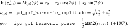
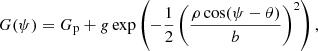
Although the IPD procedure used in Gaia DR3 does not fit for multiple peaks or non-point-like source structure, it does populate several useful statistics in the gaia_source table that give information about possible perturbations (Lindegren et al. 2021, Sect. 5). Gaia early data release 3 (EDR3) and DR3 include the following four IPD-related statistics: (1) ipd_frac_multi_peak: the percentage of windows, κ, for which the IPD algorithm has identified more than one peak, computed for all transits in which the IPD was successful. When processing each window, the IPD masks (suppresses) these secondary peaks, which typically allows for a better fit to the main peak. (2) ipd_frac_odd_win: the percentage of transits with truncated windows or multiple gate, computed for all transits in which the IPD was successful. This means that the target is likely disturbed by a brighter source close by. (3) ipd_gof_harmonic_amplitude, measuring the amplitude, aipd, of a model of the IPD goodness of fit (GoF,  ) as a function of the position angle of the scan direction; see Eq. (1) below. (4) ipd_gof_harmonic_phase, measuring the phase, φipd, of the variation of the IPD GoF (
 ) as a function of the position angle of the scan direction; see Eq. (1) below.
As described in the Gaia DR3 archive documentation (Sect. 20.1.1 of van Leeuwen et al. 2022), these two last parameters relate to a sinusoidal model fit to the natural logarithm of the IPD reduced χ2 (determined for each CCD observation) as function of scan angle, ψ, for the observations used in the astrometric solution,
 (1)
(1)
As explained in Sect. 3.1.1, the  for brighter sources (G ≲ 13) relates to a fitting using a two-dimensional PSF, and for fainter sources, it leads to a one-dimensional LSF fitting. When two sources blend, we obtain biased image parameters and a high value for the goodness of fit. This happens more easily for LSF fitting where we cannot benefit from the separation of the sources in the across-scan direction.
The main assumption in this model is that the source image to first order is axis-symmetric with respect to a certain line on the sky, parametrised by ipd_gof_harmonic_phase, which can be interpreted as the scan angle (±180°) corresponding to the worst fit. The interpretation of this direction is not straightforward. For a close binary, not detected as such by the IPD (and thus unresolved, following the nomenclature introduced at the end of Sect. 3.1), the worst fit will be along the line joining the two sources, known as the position angle. For these unresolved pairs, ipd_frac_multi_peak will be small (typically, a secondary peak is detected in fewer than 10% of the windows). This situation will happen for separations ≲0.1″. On the other hand, for a somewhat wider binary (partially resolved), the two peaks are best detected when scanning along this line, and because the secondary signal is then suppressed, this is where we obtain the best fit. For these pairs, and especially for resolved pairs, ipd_frac_multi_peak will be high (around 30 to 50%, perhaps even approaching 100% if the secondary peak is detected in nearly all scans). In this case, ipd_gof_harmonic_phase differs from the position angle of the binary (modulo 180°) by approximately ±90°. For galaxies, the angular extent is also important, but typically, the disk will be interpreted as high background by the IPD when scanning along the major axis, and this will then be the direction of the best fit. Here, ipd_gof_harmonic_phase will also differ from the position angle of the major axis (modulo 180°) by approximately ±90°.
The exact scan-angle dependence on the logarithm of  will obviously not always be well-characterised by a sinusoidal model, but it nonetheless provides us with a very useful first-order model that allows us to know the amplitude and direction (phase) of the distortion. The reference level c0 of Eq. (1) is not published.
Fabricius et al. (2021) and Gaia Collaboration (2023a) showed that the ipd_gof_harmonic_amplitude and ipd_gof_harmonic_phase are useful for identifying spurious solutions of resolved doubles. As of Gaia DR3, these are not yet correctly handled in the Gaia astrometric processing. Even though IPD is able to detect secondary peaks in the windows, no PSF or LSF fitting is attempted for them, which also means that they are not cross-matched to any source. In Sect. 6.4 we discuss the values of the IPD statistics (and others) in more detail that might be significant in relation to scan-angle-dependent signals.
We concentrated on explicit scan-angle-dependent biases from the IPD. These biases will lead to poorer astrometric and photometric solutions and will to some extent be reflected in the various astrometric and photometric quality indicators in gaia_source.
3.1.3. Demonstration of scan-angle-dependent signals resulting from IPD outputs
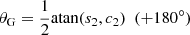
As explained in Sect. 3.1.1, IPD model errors can arise from multi-peak or non-point-like (extended) sources. The latter is also clearly demonstrated in Gaia Collaboration (2023b) for galaxies that are extended by definition. Figure 6 illustrates the main concepts involved here, such as the pixel size and proportions, the PSF, the scan angle, and the separation between the two components of an optical binary star. The Gaia scan angle is defined as ψ = 0° when the field of view is moving towards local north, and ψ = 90° towards local east, which is different from that used for HIPPARCOS (for example van Leeuwen 2007). In the following, we illustrate the main three cases described in the detailed description of ipd_gof_harmonic_phase2. All examples shown in this study are also summarised in Table 1.
 |
Fig. 6. Sky-projected illustration of the rough zones in which equal-brightness optical binary stars (two red crosses) at angular separation ρ and position angle θ can be resolved by Gaia. In the partially resolved region, the stars are resolved into two components depending on the scan angle ψi of the observation i, because of the asymmetric PSF, which has the highest spatial resolution in the along-scan direction. The bottom right inset shows a typical PSF profile (Fabricius et al. 2016) that is rotated and scaled in the background image to represent the expected PSF of the upper right component of the binary star for the given scan angle. East direction (increasing RA) is towards the left. |
Overview of source examples in this work that have scan-angle-dependent signals, along with diagnostic statistics and fitted parameters.
Case 1. A double star with separation ≲0.1″, where the GoF is expected to be higher (worse) when the scan is along the arc joining the components than in the perpendicular direction, and the ipd_frac_multi_peak should be small. Figure 7 shows an example of a partially resolved binary with the scan angle, IPD, and photometric signals. We make use of some internal information provided by the intermediate data updating system (IDU; see Fabricius et al. 2016) during its initial runs for the Gaia data release 4 (DR4), and some unpublished data of DR3. The r values in the title are Spearman correlations introduced in Sect. 6, which help determine whether this is a scan-angle-dependent signal, which in this case is very likely given that both correlations are close to 1. The top panel lists the published ipd_gof_harmonic_amplitude, ipd_gof_harmonic_phase, and ipd_frac_multi_peak as aipd, φipd, and κ, together with the time series of the IPD goodness of fit (per CCD observation) differentiated between observations detected as single peak or multiple peaks. The central panel shows the derived photometry (per field-of-view transit) in G, GBP, and GRP. For G we include two fits to the data that are detailed in Sect. 5: (1) a Pair fit (Eq. (4)), which is a generalisation of Eq. (1), leading to magnitude estimates for the primary and secondary components (Gp and Gs), their separation ρ, and their position angle θ; and (2) a small-separation simpler Sine fit (Eq. (5)) that has the same parametrisation as Eq. (1) and whose amplitude aG is comparable to that of aipd (although with a different unit); see also Fig. A.6. Depending on the separation, the phase θG is ±90° offset to φipd (as is the case here) or similar in value. This second simpler model can perform better than Eq. (4) for small separations, especially when the secondary peak is never resolved, and it is provided for all photometric sources with available time series in Appendix A. The goodness of both fits is indicated as  . The bottom panel shows an approximate reconstruction of the source environment using the source environment analysis pipeline, SEAPipe (Harrison 2011, see also Sect. 7.6). In this example, as in many other cases with partially resolved pairs, AGIS was unable to determine a full solution, and therefore only a two-parameter solution is available in DR3. As can be seen, the G-band photometry strongly depends on the scan angle, with fainter values for the scans in which IPD was able to detect and mask the secondary peak (labelled “Multi” in the top panel). In the unresolved scans (“Single”), both peaks are combined in the IPD fitting, leading to an artificially brighter value. In this case, the separation is large enough to allow for a rather high κ of 29% and a good fit with the pair model. Photometry from the blue and red photometer instruments (BP and RP, respectively) is mostly constant because of the larger windows used there. Finally, the lower (better) epoch GoF values are found in the scans in which the two peaks are not resolved, as expected. For completeness, the central panel also includes the G-band observations that were rejected during variability processing and excluded from our fitting procedure, that is, with variability_flag_g_reject = true.
 |
Fig. 7. SourceID 389636619892245248: Scan-angle signatures from a partially resolved double star with similar magnitudes and a separation of about 130 mas between the two components (determined by IDU for DR4). The top panel shows the unpublished IPD epoch GoF values determined by IDU in DR3, where we indicate the scans for which the IPD detected multiple peaks. The central panel shows the brightness in the G band and in the BP and RP photometry as provided by the epoch-photometry table published in DR3, to illustrate the differences in that instrument. It also includes the fits to G using Eq. (4) (pair model) and Eq. (5) (sinusoidal model). The bottom panel shows the image reconstructed by SEAPipe, with dashed grey circles at increasing radii in steps of 250 mas from the image centre. See text for further details. |
Case 2. A resolved binary, in which the GoF is expected to be smaller (better) when the scan is along the arc joining the two components (along the position angle), and the ipd_frac_multi_peak value should be high. Figure 8 shows an example that again shows strong variation in G-band photometry with the scan angle. With this larger separation, Eq. (4) fits the signal much better than Eq. (5). In this case, depending on the epoch, this source is assigned one-dimensional or two-dimensional windows because its magnitude is close to 13. The G-band photometry again becomes brighter, especially when the IPD is unable to detect the secondary peak, and vice versa. The separation is still too small to cause any significant variations in the larger BP and RP windows, meaning that these bands will contain the contribution from both sources. For the epoch IPD GoF, better fits (lower values) are obtained when the IPD detects and masks the secondary source, as expected. This typically occurs when the scan is made along the arc joining the two components. The value of κ (84%) is very high.
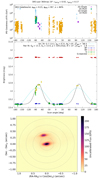 |
Fig. 8. SourceID 382074694311961856: Scan-angle signatures (top and central panels) and image reconstructed by SEAPipe (bottom panel) from a resolved double star with a separation of about 360 mas between the two components, available as two separate sources in DR3 (only one of the two sources is shown in the top and central panels). See text and Fig. 7 for further details. |
Case 3. A galaxy with elongated intensity distribution, for which a smaller GoF is expected when the scan is along the major axis of the image. Figure 9 shows an example for a galaxy candidate with G-band magnitude around 20, two-parameter AGIS solution, and the following de Vaucouleurs fitted parameters (Ducourant et al. 2023): radius 1.65″, ellipticity 0.35, and position angle 63.4°. ipd_gof_harmonic_phase takes a value of about 150°. The predicted difference is nearly 90° with respect to the correctly fitted position angle θG. This time, the variations in GBP and GRP photometry are significant because the source is very extended, as further explained in Sect. 3.2. This also causes the GBP and GRP to be brighter than the G. On the other hand, κ is zero, as expected, since this smooth extension of the source cannot be identified as secondary peaks by the IPD (except in one single transit, which was probably a spurious detection). The pair model is obviously not applicable here: after the maximum number of iterations allowed is exceeded, the best fit indicates an unrealistically low ρ value of 46 mas.
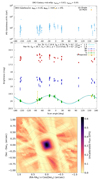 |
Fig. 9. Galaxy LEDA 2112767 (Paturel et al. 2003), sourceID 366951667785042688: Scan-angle signatures (top and central panels) and image reconstructed by SEAPipe (bottom panel). This galaxy was published in Gaia DR3 with a moderate ellipticity. See text and Fig. 7 for further details. |
Appendix B provides additional examples for the different cases. In general, the G-band photometric signal in magnitude is well modelled by Eq. (5) (which is identical to the IPD model of Eq. (1)), although there can be exceptions where Eq. (4) performs significantly better. These models seems to provide better fits on photometry than on the IPD GoF, although ipd_gof_harmonic_amplitude typically provides a reliable indication of scan-angle-dependent astrometric signals for the source. Combined with ipd_frac_multi_peak, it is a quite powerful tool for detecting extended sources or multiple point-like sources. In addition to these published quantities, Eq. (4) seems to provide very interesting fits in case of moderate separations, even allowing us to localise a neighbouring source with quite some reliability.
To further illustrate the usefulness of these IPD-related published parameters, Fig. 10 presents the density plot of the comparison of ipd_gof_harmonic_phase with the position angle for ∼914 000 galaxies measured by the Gaia surface-brightness profile fitting pipeline of the extended objects processing in the fourth coordination unit, CU4-EO (Ducourant et al. 2023; Gaia Collaboration 2023b). The two parameters agree very well (with a 90° shift, as previously explained). Sources that depart from the dense lines are quasi-circular galaxies for which the position angle is meaningless.
 |
Fig. 10. Comparison of the position angle of extended galaxies measured with Gaia data with the ipd_gof_harmonic_phase parameter. |
All G, GBP, and GRP photometry shown in this study is as published in Gaia DR3 (Riello et al. 2021; Evans et al. 2023) (unless otherwise stated). The observations flagged by the variability analyses of Eyer et al. (2023) were rejected, that is, observations with variability_flag_g_reject = true in the epoch-photometry time-series data.
3.2. Scan-angle-dependent signals in the blue and red photometer instruments
The BP and RP instruments measure a low-resolution spectrum (R ∼ 60) in the blue [300−700] nm and red [600−1100] nm part of the spectrum. For a detailed description of the instrument, we refer to Sect. 3.3.6 of Gaia Collaboration (2016). The integration of the flux within the window (aperture photometry) in the two photometers generates the GBP and GRP magnitudes. Because no LSF or PSF fitting is involved to process the data, it is less likely to introduce scan-angle-dependent model errors due to subtle LSF or PSF mismatches. However, scan-angle-dependent model errors can still be introduced through blending because the BP and RP spectra are acquired with windows that are much wider than those used for the AF observations in the AL direction, with a length of 60 pixels, corresponding to ∼3.5″. This means that more blending is expected to occur in BP and RP than in G, especially in crowded regions. How strong the crowding effect is depends on the separation between sources, but also on the scan angle, as the amount of flux from the blending source will vary depending on the mutual position of the sources and the scanning direction. An example is shown in Fig. 11.
 |
Fig. 11. Example of two sources causing blended spectra in some of the observations. The rectangular shapes show the footprint of the observing window for real transits over one of the two sources. In the transits highlighted in green, the secondary source is located beyond the window, while both sources are inside the window for grey transits. The dispersion direction is along the major side of the observing window. |
The GBP and GRP magnitudes are calculated by integrating the respective spectra, and because no deblending correction has been applied in DR3 yet, they can be affected by crowding. In Sect. 6 of Riello et al. (2021), the corrected BP and RP flux excess C* for the photometry was defined. C* is a consistency metric for the mean photometry, and it depends on the G, GBP, and GRP fluxes and the colour. We have computed the equivalent C* from epoch photometry. Figure 12 shows some examples of the variation in epoch-flux excess C* as a function of the epoch photometry. In some cases (green crosses and yellow diamonds), C* correlates with G, but it does not depend on GBP and GRP: here the two sources are close enough that every BP and RP transit contains the flux of both sources, while the amount of flux in the AF varies with the scan angle. In the other cases, GBP and GRP are instead correlated with C*, indicating that the amount of flux in BP/RP varies with the scan angle, while in G, the two sources are distant enough to prevent contamination, and G is not affected or it is affected only negligibly. The crowding evaluation was carried out in the BP/RP processing, and the crowding status in the plots is relevant only for those instruments. While the examples represent only a handful of cases, the bottom panel of Fig. 19 in Riello et al. (2021) shows this effect in a more global way: The corrected BP and RP flux excess with the colour of the sources colour-coded by blend probability clearly shows that C* is closer to zero (indicating good and consistent photometry) when the blend probability is lower than 20%.
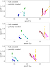 |
Fig. 12. Examples of crowding effects on the photometry for six sources, each with a different colour. From top to bottom, we show the epoch-corrected flux excess C* as a function of epoch G, GBP, and GRP. Sources shown as crosses were estimated as crowded in every BP/RP transit. Sources shown as diamonds were estimated as crowded in only a few transits. |
The examples in Fig. 12 show that sources can be strongly correlated between the epoch-corrected flux excess C* and photometric G, GBP, and GRP. We quantify this correlation using three Spearman correlations: rexf, G, rexf, BP, and rexf, RP, as detailed in Sect. 6.2 and published with this paper for all sources with published photometric time series in Gaia DR3 as described in Appendix A.
3.3. Radial velocity spectrometer
The radial velocity spectrometer (RVS; Cropper et al. 2018) produces high-resolution spectra (R ∼ 11 500) of sources between 845 and 872 nm. The light of sources observed by the RVS is dispersed (0.0245 nm pixel−1) by a grating plate, resulting in a spectrum that spreads over about 1100 pixels in the AL direction, corresponding to 65 arcsec. The RVS focal plane is composed of 12 CCDs arranged in four rows.
The wavelength range of RVS spectra contains, amongst other possible lines, the calcium triplet, which allows measuring the radial velocity for a wide range of stellar types. The RVS instrument is aimed to estimate the mean radial velocity (RV) at the end of the mission for basically all stars up until GRVS ∼ 16, and to provide time-series RV data up until GRVS ≲ 13.
3.3.1. Scan-angle-dependent signals in RVS data of astrometric binaries
The RVS does not have any internal calibration source to perform a wavelength calibration of individual spectra. The wavelength values are associated with each sample of a spectrum, assuming that the wavelength is a polynomial function of the field angles (η, ζ) of the source, that is, the position of the source in the FoV reference system (FoVRS; see Lindegren et al. 2012, for the definition of this reference system), at the time at which the sample crossed the fiducial line of the CCD. The coefficients of the above function are quantities that evolve slowly in time, and they are determined using the observations of bright stars with known radial velocity (see Sartoretti et al. 2018, for more details).
In the RVS DR3 processing, the field angles of the observed source are computed from the single-star astrometric parameters determined by AGIS (Lindegren et al. 2012). If the real position of the source in the FoVRS is different from the predicted position, the wavelength associated with the spectrum samples will be incorrect. This mismatch can be due either to a problem in the AGIS astrometric parameters of the source or to the astrometric motion along the Keplerian orbit of the star in the case of an astrometric binary. Because the RVS dispersion occurs in the AL direction, the effect of a mismatch in the position is at first order proportional to Δη, that is, the displacement projected on the AL direction. The effect on the epoch radial velocity (that is, the difference between the measured and the real RV) will be ΔRV = −0.146 ⋅ Δη, with ΔRV in km s−1, and Δη (in mas) being the difference between the real and the assumed η value.
An example of the effect of the astrometric orbit on the epoch RV of an astrometric binary, Gaia DR3 6631710606341412096, is shown in Fig. 13. The AstroSpectroSB1 solution of this source has an orbit with period of 937.0 days, a semi-axis a0 = 11.79 mas, and a parallax of 25.98 mas. See Gaia Collaboration (2023a) for the description of non–single–star (NSS) solutions. In the top panel of Fig. 13, we show the position of the source on the sky in the reference system moving with Gaia, as predicted from the AGIS single-star astrometric solution, compared with the position predicted when the astrometric orbit is included. The bottom panel shows the epoch RV data, folded in phase, as provided by the DR3 pipeline (blue dots), and the data corrected for the displacement (in red), compared with the AstroSpectroSB1 solution.
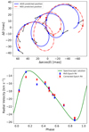 |
Fig. 13. Example demonstrating how insufficient astrometric modelling leads to incorrect RV determinations. Top panel: motion of Gaia DR3 6631710606341412096 on the sky with respect to its reference position in the reference system moving with Gaia, as predicted from the five-parameter single-star AGIS solution (solid blue line), compared with the position predicted by the NSS AstroSpectroSB1 solution (dot-dashed red line), which included the Keplerian orbit. Circles show the positions at which the epoch RV were measured, and the arrows show the scanning direction at the epoch. Bottom panel: RV data, folded in phase, as provided by the DR3 pipeline (blue dots) and the data corrected for the displacement (in red), compared with the radial velocity predicted by the AstroSpectroSB1 solution (green line). |
The bottom panel of Fig. 13 shows that the effect of the astrometric orbit on the epoch RV (not published in Gaia DR3) can, as a consequence, produce an NSS solution that is not fully correct. In the case of Gaia DR3 6631710606341412096, which was chosen from those in which the effect is strongest, the semi-amplitude of the RV curve is certainly affected, but not dramatically so. The semi-amplitude is the most affected spectroscopic orbital parameter, but the eccentricity (and the argument of periastron) might also be sensitive. However, the spectroscopic values are certainly not predominant in the combined orbital solution; the dominant constraints always come from the astrometry.
It should be noted that this effect is weaker than the epoch RV errors for the vast majority of the astrometric binaries detected by Gaia, and it is relevant only for nearby and bright astrometric binaries with a large semi-axis orbit. Using the orbit semi-axis from the published non-single star (NSS) Orbital and AstroSpectroSB1 solutions as estimate of the maximum expected Δη, we found that 1876 sources with AstroSpectroSB1 and 1024 sources with Orbital solutions have an effect on the epoch radial velocity that is stronger than the mean of epoch RV errors. The means of epoch RV errors are not published in Gaia DR3. A correction of this problem is planned for the next release.
3.3.2. Scan-angle-dependent signals in RVS data of non-point-like sources
The second situation in which the epoch radial velocities of a source receive a spurious signal that depends on the scan angle is when the source is a resolved or partially resolved binary or double star. The meaning of resolved or partially resolved is discussed in Sect. 3.1.2.
If the onboard software is not able to distinguish the two stars composing the source, a single window is generated when the source is observed. In this case, the RVS pipeline is not able to deblend the overlapping spectra of the two components, and the spectra will be processed as if it were a single star.
The absorption lines of the two components in the processed spectra will appear shifted in wavelength with respect to their expected position, proportionally to the displacement with respect to the predicted position in the FoVRS, projected on the AL direction, according to the relation ΔRV = −0.146 ⋅ Δη described in the previous section.
The RVS pipeline includes an implementation of an algorithm similar to the two-dimensional correlation technique, TodCor (Zucker & Mazeh 1994; Damerdji et al., in prep.) to identify double-lined spectra. As described in Damerdji et al. (in prep.), the algorithm has limits: When the source is fainter than GRVS = 11, or when the faintest component is more than five times fainter than the primary, or when the RV separation between the lines of the two components is below 15 km s−1, the RVS pipeline is unable to identify the spectrum as double lined.
When the blended spectra are not detected as double lined and the two components have similar radial velocities (for example, as expected in wide binary systems), the blending will result in a shift of the position of the centroid of the absorption lines. This will generate a radial velocity signal that is proportional to the separation projected on the AL direction. The spurious signal will be
 (2)
(2)
where the semi-amplitude K depends on the separation, the luminosity ratio, and the respective spectral types, while ψ and θ are the scan angle and the position angle of the secondary, respectively. Because the scanning angle has the same periodicity as the spacecraft precession, this will generate spurious NSS SB1 solutions with a similar period, as noted in Gaia Collaboration (2023a).
An example of a spurious SB1 solution due to a resolved binary is Gaia DR3 5648209549925093504. This source, as revealed by SEAPipe preliminary results shown in the top panel of Fig. 14, is composed of two stars that are separated by about 300 mas. This source has ipd_frac_multi_peak = 90 and ipd_gof_harmonic_phase = 66.4°. As explained in Sect. 3.1.3, we obtain a position angle θ ∼ ipd_gof_harmonic_phase − 90° = 336.4°, which agrees well with what is seen in the SEAPipe image.
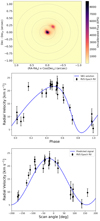 |
Fig. 14. Top panel: image of the source Gaia DR3 5648209549925093504 produced by SEAPipe. Middle panel: RV data of Gaia DR3 5648209549925093504, folded in phase, as provided by the DR3 pipeline (black dots), compared with the SB1 solution provided in DR3 (blue line). Bottom panel: RV data as a function of the scan angle ψ, compared with a sinusoidal signal as predicted by Eq. (2). |
The middle panel shows the epoch RV data, folded in phase, compared with the published SB1 solution. In the bottom panel, the epoch RV data, folded with the scan angle, are compared with the RV predicted by Eq. (2), and with K equal to the semi-amplitude of the SB1 solution. The measured RV variability is well reproduced by the scan-angle effect. This proves that this is a spurious SB1 solution. An algorithm that can identify spurious solutions like this is planned for the next release.
When the TodCor algorithm identifies the spectra as double lined, the source might be identified as a double-lined spectroscopic binary (SB2) by the NSS pipeline, with a period near the precession period. We found no spurious SB2 solution in the DR3 data.
3.3.3. Scan-angle-dependent signals in RVS data due to contamination
A third type of scan-angle-dependent signal is introduced by the contamination of a spectrum with the light from a nearby source (see Seabroke et al. 2021; Boubert et al. 2019). The RVS pipeline for DR3 (Katz et al. 2023) contains a deblending algorithm (described in Seabroke et al. 2021) that treats the case of overlap of windows of two (or more) sources. When a source is bright enough, however, its light can contaminate the spectra of nearby fainter stars even if their windows do not overlap. As discussed in more detail in Katz et al. (2023), the RVS pipeline for DR3 is not able to identify such cases. During the DR3 validation phase, a method was identified to filter out these cases, although it was only applied to the mean radial velocity. The epoch RVs of some contaminated stars were instead processed in the NSS pipeline, generating occasionally spurious SB1 solutions. One example is Gaia DR3 2006840790676091776, which is a G = 11.18 source that is contaminated by Gaia DR3 2006840790679122688 (G = 3.86) at 31.9 arcsec.
In Fig. 15 we show the spectrum of Gaia DR3 2006840790676091776, recorded in one of the contaminated transits. At wavelengths shorter than 859 nm, the spectrum is dominated by the light of the contaminating bright source Gaia DR3 2006840790679122688. The shoulder at 859 nm corresponds to the red limit of the transmission band associated with the contaminating source (and thus shifted by some 12 nm here). The solid vertical red lines show the real position of the Ca II triplet lines of Gaia DR3 2006840790676091776. The presence of the Ca II 866.452 nm from the bright contaminating source (thus also shifted) near the Ca II 854.444 nm line of the contaminated source produces a peak in the cross-correlation function when the spectrum is compared with the template (see Sartoretti et al. 2018, for details about the RV derivation), resulting in an incorrect RV.
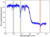 |
Fig. 15. Spectrum of Gaia DR3 2006840790676091776, contaminated by the nearby source Gaia DR3 2006840790679122688 recorded in a transit. The solid vertical red lines show the real position of the Ca II triplet lines of Gaia DR3 2006840790676091776, and the dot-dashed green lines show the position of the same lines as found by the pipeline. |
4. Spurious periods in Gaia data
4.1. Observed period structure
A clear feature observed during the data processing for Gaia DR3 is that specific periods are identified much more frequently than others. This is illustrated with several public and non-public data sets in Fig. 16. The first set (top panel) is drawn from a (unpublished) sample of about 1.6 million sources that were selected by randomly sampling from the full range of magnitude in the G-band photometric data, with an upper limit of 6000 objects per 0.05 mag interval, and then by filtering out sources with fewer than five FoV transits in the G band and those without any measurement in both GBP and GRP. They were then processed by the default variability pipeline of Eyer et al. (2023), in which only sources were selected that passed a general variability test. An unweighted periodogram was then made using generalised least-squares (Heck et al. 1985; Cumming et al. 1999; Zechmeister & Kürster 2009) (an extension of the Fourier periodogram on unevenly sampled data that is independent of the mean of the data), followed by a refinement of the period with the highest power using an unweighted multi-harmonic modelling step. The periodogram was computed between 25 cycles day−1 (about 1 h) and 7 × 10⁻⁴ cycles day−1 (1700 d), with a step size of typically 10−5 cycles day−1. We only display the 73 k sources with periods in the range 10−500 d in which most of the easily identifiable spurious peaks appear.
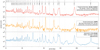 |
Fig. 16. Period distributions of (largely unpublished) Gaia data to show the diversity and (dis)similarities of various peak locations and amplitudes. See also Figs. 22–24 for comparison with period search results on simulated scan-angle signals that qualitatively reproduce these peaks. |
The second set (middle panel) is extracted from the public photometry published as part of the Gaia Andromeda photometric survey (GAPS; Evans et al. 2023). Periods and false-alarm probabilities are provided in Appendix A. The same processing and selections as for the first set were applied, resulting in 38 k sources with periods in the range 10−500 d, as shown. For the first and second dataset, we show in Fig. 17 the Baluev false-alarm probability (FAP; Baluev 2009). The FAP shows that a significant fraction of the peaks is highly significant. As a result of the initial blind source selection, both sets will contain a mix of truly photometric variable objects and spurious variables (for example galaxies and close pairs) due to induced scan-angle-dependent signals or other disturbances in the Gaia data. Most sources of each data set will not exhibit any (periodic) variability at all, however.
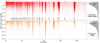 |
Fig. 17. Distribution of false-alarm probabilities of the two photometric samples shown in Fig. 16, illustrating the highly significant nature of most of the spurious periods. |
In Fig. 16, the third set (bottom panel) is a set of 1.8 million unpublished astrometric orbital solutions produced by the exoplanet pipeline on a set of stochastic sources (for details, see Sect. 5.1.1 of Holl et al. 2023).
As already illustrated by the vertical period-lines in Figs. 16 and 17 and in the figures in following sections, the positions of the main peaks are approximately centred on periods P [d],
 (3)
(3)
where 5.8 cycles yr−1 (about 63.0 d) is the precession frequency of the spin axis around the Sun during the nominal scanning law discussed in Sect. 2. The symbol n marks the number of cycles yr−1. In clearly identifiable peaks (in the marked range above 13 days), n varies from about −3 to 5. m marks the number of cycles per precession period, which starts at 0 and increases towards shorter periods (only illustrated until m = 4, but continuing beyond).
The strength and significance of the peaks significantly depends on the ecliptic latitude, which explains the difference between the top two panels of Figs. 16 and 17. This is explored in detail Sect. 5.4 and in the associated sky plots in Appendix C.
4.2. Interpreting the period peak structure
As remarked in Lebzelter et al. (2023), this structure might be interpreted as some sort of aliasing of the combined periodicities. However, the term aliasing is misleading because in this case, the signal consists of a frequency in the scan-angle domain that is mapped onto the time-domain through a sky-position-dependent transformation encoded in the NSL, in contrast to the usual aliasing (the sample aliasing), where a true frequency in a frequencygram is distributed over different frequencies due to a convolution with a specific window function. A full analysis of the origin of Eq. (3) and the resulting prevalence of expected frequencies is beyond the scope of this paper, but it might be thought of as the combined effect of different harmonics of the yearly and spin-axis period of the satellite, where the power in the harmonics comes from the deliberate non-integer fraction of cycles per year of the precession frequency, to randomise both scan-angle orientations and observation times. In addition, lower-order perturbations come from the non-constant precession phase-rate discussed in Sect. 2.1, which is also further complicated by the slightly elliptical orbit around the Sun.
These same period locations relate to expected variations in the selection function of photometric periodic sources and astrometric orbits and in the derived-parameter biases (see for example Lindegren 2022; Penoyre et al. 2022), which undoubtedly also affect the shown samples. They are part of the expected features of the data sampling and adopted source model parametrisations, however, which is not the subject of this particular study and thus is not discussed further in this paper. We do not show the period distribution below 10 d (which is only an aesthetic choice to focus on the clearest longer-period peaks), but photometric spurious peaks from scan-angle-dependent signals have been identified down to much shorter periods, and thus higher m. For example, about 1000 galaxies that were misclassified as RR Lyrae stars with periods of about 0.3 d were already identified in Gaia DR2 data (see Table C.1 of Clementini et al. 2019).
5. Simulated scan-angle signals and spurious periods
We start in Sect. 5.1 to numerically simulate the expected scan-angle-dependent bias signal in the photometric magnitudes and astrometric AL-scan centroids of the sources, mimicking those introduced through the mechanisms explained in Sect. 3. Next we provide analytical expressions for these bias signals in Sects. 5.2 and 5.3, respectively. Finally, in Sect. 5.4, we use harmonic decompositions of these analytical expressions to simulate how they propagate in the derived photometric period and astrometric (orbital) parameters when left unmodelled (as is the case for Gaia DR3), and compare them qualitatively with the observed distributions in Gaia data introduced in Sect. 4.1.
5.1. Numerical simulation of the scan-angle bias
We made a simple numerical simulation of the observation of two close sources in different scan directions in order to determine how much the observed position and magnitude of the brighter source is biased by the presence of the fainter neighbour. The simulation was noise free and used a realistic LSF, and it assumed the data processing does not suppress the signal from the fainter source. We simulated five different separations (10, 50, 100, 200, and 400 mas) and two different magnitude differences (0.5 and 2.5 mag). The result is shown in Fig. 18 for the observed magnitude and in Fig. 19 for the observed position. We note that the dependence on scan angle has a similar overall appearance for both magnitude differences, but the amplitude strongly depends on this difference.
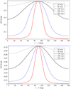 |
Fig. 18. Simulation of the magnitude bias, ΔG, for the brighter component of a close source pair for five different separations and as a function of the difference between the position angle of the scan and the position angle of the fainter component. The magnitude differences in the top panel are 0.5 mag and in the bottom panel 2.5 mag. |
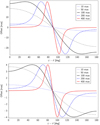 |
Fig. 19. Simulation of the positional bias for the brighter component of a close source pair for five different separations and as a function of the difference between the position angle of the scan and the position angle of the fainter component. The magnitude differences in the top panel are 0.5 mag and in the bottom panel 2.5 mag. |
When scanning at 90° relative to the position angle of the pair, the two images will overlap and we obtain the brightest flux in photometry and no effect in position. As the scan angle moves away from 90°, the effect in flux diminishes and more rapidly so for the larger separations. In position, the effect is strong as long as the two images partly overlap, and it then diminishes. The positional biases shown in Fig. 19 represent the offset in the scan direction from the position of the brighter component. In practice, for a source pair separated by less than about 50 mas, the observed position will represent the photocentre, and the variation with scan angle in the observed position with respect to the photocentre will be much smaller than the variation with respect to one of the components. For large separations, the data processing will detect the fainter source as soon as the relative scan angle is sufficiently far from 90° and will reduce its influence. The observed position will therefore not be quite as strongly affected as the figure may suggest. Depending on how observations are distributed in time and in position angle, the biased positions will distort the astrometric solution differently. The astrometric residuals with respect to this distorted solution will therefore not have the simple form shown in the figure, and this is further discussed in Sect. 5.3.
5.2. Analytical expression for photometric bias
It is clear from Fig. 18 that we can expect a star pair to produce a significant variation in the observed G magnitude with scan angle. The form and phase of this variation will strongly depend on the separation, the magnitude difference, and the position angle of the source, so that we can even estimate these three parameters from the light curve, except for a 180° ambiguity in position angle. On the other hand, following Sect. 3.2, for GBP and GRP, we do not expect a significant scan-angle dependence as long as the separation is small enough for the spectra of the two sources to be contained within the observing window.
We obtain a crude representation of the simulated variation of the observed magnitude with scan angle from the following expression, which is inspired by the discussion in Lindegren (2022):
 (4)
(4)
where
-
Gp is the magnitude of the primary component,
-
g = −2.5log(1 + 10−0.4(Gs − Gp)),
-
Gs is the magnitude of the secondary component,
-
ρ is the angular separation of the pair,
-
θ is the position angle of the secondary,
-
ψ is the position angle of the scan, and
-
b is a measure of the width of the LSF.
This can only serve as a first approximation. The problematic quantity is the width, b, which takes lower values for larger magnitude differences, where the secondary only has a small effect on the image shape. For the simulations shown in Fig. 18, values of b = 74 mas and b = 90 mas are representative for the larger and smaller magnitude difference, but we expect that higher values are needed for the actual observations. We have used b = 100 mas in the fits shown in Figs. 7–9 and tabulated in Table 1.
We note that the fundamental frequency of Eq. (4) is at twice the scan angle (as seen next in Eq. (5)) and that higher harmonics are implicitly constrained to even multiples of the scan angle. This is a relevant observation when the propagation of this bias signal into a period-detection algorithm is simulated in Sect. 5.4, where we sample several harmonic components separately. It is important to point out that we adopted the simplified assumption that the position angle does not significantly change over the mission duration and thus can be considered constant. Taking changing position angles into account would cause non-trivial distortions of the induced signal that are beyond the scope of this work.
5.3. Photometric bias model at small separations
For small separations relative to the LSF width, the expression in Eq. (4) can be approximated with the sinusoidal expression that was introduced in Eq. (1) to fit the natural logarithm of the IPD goodness of fit, which is therefore also adequate for modelling the affected G photometric signal,
 (5)
(5)
where
-
 ,
, -
 ,
, -
 .
.
From these coefficients, we find
-
 ,
, -
 ,
,
where aG is the amplitude of the magnitude variation.
We note that for a given amplitude of the sinusoid, the brightening in magnitude, g, from adding the secondary source is inversely proportional to the square of the separation.
5.4. Analytical expression for astrometric AL-scan bias
A detailed study of the astrometric bias and its effect on detection of astrometric binaries can be found in Lindegren (2022), from which we adopt the analytical expression for the astrometric AL-scan bias relative to the barycentre (their Eq. (12)),
![Mathematical equation: $$ \begin{aligned} \delta \eta = {\left\{ \begin{array}{ll} \left({\displaystyle \frac{f}{1+f}}-{\displaystyle \frac{q}{1+q}}\right) \Delta \eta&\mathrm{if\,|\Delta \eta /u|\le 0.1,}\\ [12pt] uB(f, \Delta \eta /u) - {\displaystyle \frac{q}{1+q}}\,\Delta \eta&\mathrm{if}\,0.1<|\Delta \eta /u|\le 3-f,\\ -{\displaystyle \frac{q}{1+q}}\,\Delta \eta&\mathrm{if}\,3-f < |\Delta \eta /u|, \end{array}\right.} \end{aligned} $$](/articles/aa/full_html/2023/06/aa45353-22/aa45353-22-eq19.gif) (6)
(6)
with f and q the flux and mass ratio, respectively, in the sense fainter divided by brighter. The bias is primarily a function of the projected AL separation Δη = ρcos(ψ − θ), with ρ the binary separation and θ the position angle of the binary. B(f, x) is the dimensionless anti-symmetric bias function (that is, B(f, −x) = − B(f, x)) introduced in their Appendix E, and u = 90 mas is the resolution unit of the instrument. In Fig. 20 we illustrate the shape of the δη AL-scan bias as a function of the scan angle for a fixed-orientation binary (P ≫ 5 y) with θ = 0°, mass ratio q = 0.9, flux ratio f = 0.656 (ΔG = 0.46), and separations varying between 100 and 400 mas. We are assuming f = q4 for non-giant binaries (Sect. 2.2, Lindegren 2022). Now, we consider the propagation of this signal into the astrometric source parameters. To first order, this signal (shown as the blue line in the top panels) is proportional to cos(ψ), which will be absorbed as a position bias (see Eq. (13) of Lindegren 2022), with the offset being the signal amplitude, and the direction determined by the position angle. The residual of this cosine signal (magenta line in the bottom panels) will be available to propagate into, and thus bias, other astrometric parameters, as we further examine in Sect. 5.4. These residual signals are usually of much smaller magnitude and are nearly proportional to cos(3ψ), while even higher odd harmonics appear for greater separations. We note that in Eq. (6), all harmonics are implicitly constrained to odd multiples of the scan angle. For completeness, we also show in Fig. 21 the bias signal induced by a typical binary with a mass ratio of q = 0.23 (Duquennoy & Mayor 1991) and a flux ratio of f = 2.8 × 10⁻³ (ΔG = 6.38).
 |
Fig. 20. Astrometric along-scan bias δη of Eq. (6) as a function of scan angle ψ for a flux ratio f = 0.656 (ΔG = 0.46, mass ratio q = 0.9), and position angle θ = 0°. Left to right: source separation ρ = 100, 200, 300, and 400 mas. Top panels: total bias δη (blue line), and a cosine fit (dashed red line) that will propagate into a position bias. Bottom panels: residuals of the cosine fit (magenta line) that can bias other source parameters. |
 |
Fig. 21. Same as Fig. 20, but for a flux ratio f = 2.8 × 10⁻³ (ΔG = 6.38), corresponding to the mass ratio q = 0.23 of a typical binary. |
5.5. Propagation of bias signals into derived parameters
In this section, we explore how a photometric bias signal as in Eq. (4) and an astrometric AL-scan bias signal as in Eq. (6) propagate into derived parameters such as the derived (orbital) period. Although the two equations look rather different, we have already identified in their originating sections that they can be decomposed into harmonics of even and uneven multiples of the scan angle, respectively, with the highest power usually residing in the lowest harmonic, as listed in Table 2. A generic expression for this harmonic decomposition is
![Mathematical equation: $$ \begin{aligned}&b(\psi )\,=\,c_0 + \sum _k c_k \, \cos k\psi + s_k \, \sin k\psi , \\&\mathrm{with} \quad k = {\left\{ \begin{array}{ll} \mathrm{even{:}\,photometric\,bias\,[mag]}\\ \mathrm{odd{:}\,astrometric\,AL\text{-}scan\,bias\,[mas]}\\ \end{array}\right.}\nonumber \\&\mathrm{and} \quad a_k = \sqrt{s_k^2 + c_k^2} \nonumber . \end{aligned} $$](/articles/aa/full_html/2023/06/aa45353-22/aa45353-22-eq20.gif) (7)
(7)
Because a full exploration of the parameter space of the original photometric Eq. (4) and astrometric Eq. (6) biases is beyond the scope of this study, we instead assess the properties of their propagated biases by simulating the noiseless scan-angle bias signal represented by each k individually, and qualitatively compare this to observed distributions of Fig. 16. We do this by simulating the signal for sources on a uniformly HEALPix sky grid for 20 uniformly spread position angles to obtain an impression of the general all-sky response. For photometry, we used a HEALPix grid level of 6 (∼49 k positions with a granularity of about 0.92′), leading to about one million simulations for each even k, and in astrometry level 5 (∼12 k positions with a granularity of about 1.8°), leading to ∼250 k simulations for each uneven k. To simulate the GAPS data, we simply analysed the subset of 113 level 6 HEALPix pixels within the defined 5.5° radius around the Andromeda Galaxy (that is, 2260 simulations for each even k).
Because we compared our simulations with the observed data samples introduced in Sect. 4.1, the representability for the two all-sky samples might be enhanced by weighting the output of our uniform all-sky simulation as function of the expected sky density. We avoided adding this complexity (and choice of prior) because the result already represents the data very well, as shown in the following sections.
In these simulations, we made the important implicit assumption that the (main) source of scan-angle-dependent signals arises because (close) pair stars around the resolving limit of Gaia have a fixed position angle on the sky for the duration of the Gaia mission data. For galaxies, we showed in Sect. 3.1.3 that their photometric signal is similar to that of unresolved star pairs (with a shift of the phase at which their scan-angle-dependent bias signal peaks), and thus they are equally well included in this simulation. The astrometric signal for galaxies has not been studied yet, but generally, the astrometric signal of galaxies is not well represented by a five-parameter model and ends up as a two-parameter solution.
5.5.1. Propagation of the photometric bias signal into period
To derive the most dominant photometric period generated by the noiseless photometric scan-angle bias signal, we used the same generalised least-squares method as discussed in Sect. 4.1, but now with a lower period limit of 1 d and no further modelling or frequency refinement. Changing the maximum frequency from 25 cycles d−1 to 1 speeds up the computation dramatically, while spurious peaks induced by scan-angle signal below 1 d occur infrequently. We only inspected periods longer than 10 d. The periodogram is insensitive to any offset because it is fitted as part of the method, and thus c0 of Eq. (7) was set to zero. This fit remained unweighted because we studied the propagation of a noiseless signal.
The top panel of Fig. 22 shows the observed Gaia period distribution of the unpublished all-sky sample introduced in Sect. 4.1. This histogram is in linear scale, compared to log scale in Fig. 16. The three panels below show the period distribution of our simulations in the range 10−500 d for k = 2, 4, and 6, as listed in Table 2. Although our simulations were not adjusted for the observed sky-distribution differences, the match with the k = 2 simulation is already strikingly good. We recall that this is (equivalent to) the small separation model of Eq. (5), which suggests that the vast majority of observed photometric spurious periods is due to close pairs with a fixed position angle on the sky. The propagation of the peaks for models with k = 4 and 6 shows that specific period peaks are additionally enhanced when the photometric scan-angle bias signal has higher harmonics (especially around 31.5 d), as is the case when the pair is partially resolved (Eq. (4)). We note that propagating the harmonics separately is not equivalent to propagating a multi-harmonic model itself, but it will highlight the type of periods that would become dominant in the periodogram if the harmonic itself were to become the dominant component of the bias signal, which is thought to be sufficient for the qualitative comparison we make.
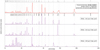 |
Fig. 22. Comparison between the unpublished observed period distribution of an all-sky photometric sample (top panel, red line, same as top panel of Fig. 16) and that predicted by our noiseless sampled bias model of Eq. (7) for different scan-angle harmonics k (purple lines in following panels). See Figs. C.2 and C.3 for ecliptic sky maps and Figs. C.4 and C.5 for spurious-period-folded time series of the most prominent peaks. |
To examine in more detail whether our simulated peaks are related to the observed peaks, we plot the position of some of the peaks of Fig. 22 on the sky and compare them with the observed sky distributions, as provided in Appendix C. In addition to the underlying density variations, the detection regions on the sky agree well. The main exception is probably the observed 182 d peak sky distribution, which appears to be not fully reproduced by our model. It might contain contributions from another calibration effect. The colour-coding also clearly shows that for |β|< 45°, the peak detection generally occurs in a relatively small fraction of the 20 sample phase steps, which is consistent with the predictions of Sect. 2.1 based on the non-uniformities in the scan-angle distribution closer to the ecliptic plane.
For the public GAPS sample, which was processed in the same way as the all-sky sample, we extracted the simulated data for the 113 HEALPix level 6 pixels within a 5.5° radius from the Andromeda galaxy (for details about the GAPS sample selection, see Evans et al. 2023). The result is shown in Fig. 23. This sample is centred around ecliptic latitude 33.4° and thus is well within the region of |β|< 45°, in which the more irregular scan-angle sampling occurs (see Sect. 2.1). The k = 2 simulation shows that the same location is generally obtained for the four highest peaks, even though the relative period distribution is not exactly reproduced. A k = 4, the 31.5 d peak might additionally be boosted by this harmonic, but we do not seem to predict the same level of boosting of the 53.7 d period as seen in the observations. Our simple simulations clearly cannot account for all detailed features, but even for such a specific sky location, it is satisfying that we detect the dominant features well.
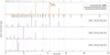 |
Fig. 23. Same as Fig. 22, but for the published GAPS photometry. The top panel (orange line) shows the same data as in the second panel of Fig. 16. The green circles in Figs. C.2 and C.3 show ecliptic sky maps of the most prominent peaks. |
5.5.2. Propagation of the astrometric bias signal into astrometric orbit
To derive the most dominant astrometric period generated by a noiseless astrometric scan-angle bias signal with an amplitude of 1 mas, we ran the genetic orbit-fitting algorithm described in the Gaia exoplanet pipeline (Holl et al. 2023) and retrieved the best-fitting Keplerian orbit. Similarly to the photometry, we simulated the response of one harmonic at a time. As listed in Table 2, these are the uneven k, starting with k = 3, and shown here until k = 7. We note that the adopted model of Eq. (6) does not contain an offset. We therefore set c0 = 0 for all simulations.
The top panel of Fig. 24 shows the observed Gaia period distribution of the unpublished all-sky stochastic sample introduced in Sect. 4.1. The three panels below show the period distribution of our simulations in the range 10−500 d for k = 3, 5, and 7, as listed in Table 2. The k = 1 simulation results in an orbital amplitude of zero because the signal is fully absorbed in the position offset. Even though our simulations were not adjusted for the observed sky-distribution differences, the match with the k = 3 simulation is promising. It contains most of the significant peaks seen in the observational data. Adding k = 5 appears to enhance the correctly identified peaks to better match the observed sample. The k = 7 simulation appears to enhance peaks that are generally not in the observed sample, however, and it might well be that this harmonic usually has very low power in the astrometric scan-angle bias signal because the companions are sufficiently well separated (and are bright enough) to be resolved individually by Gaia. This relation between higher harmonics and larger companion separation is illustrated in Figs. 20 and 21. In the same way as for the photometry, we plot the position of some of the peaks of Fig. 24 on the sky and compare them with the observed sky distributions, as provided in Appendix C. The observed and predicted location of the specific spurious periods agree well in general.
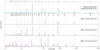 |
Fig. 24. Comparison between the unpublished period distribution of an all-sky astrometric orbit sample (top panel, blue line, same as the bottom panel of Fig. 16) and that predicted by our fits to the noiseless sampled bias model of Eq. (7) for different scan-angle harmonics k (purple lines in the following panels). See Figs. C.6 and C.7 for ecliptic sky maps of the most prominent peaks. |
To further assess the qualitative similarity of the simulations with the observed data, we additionally plot the period-eccentricity diagram in Fig. 25 (which has previously been shown in Fig. 18 of Holl et al. 2023). The overall spread of the eccentricity over the full 0−1 range in the observed data is well reproduced by our simulations (again k = 3 and k = 5 match best).
Additionally, we assess the fitted semi-major axes in Fig. 26, which for orbital fits to Gaia observations typically lie between 0.1 and 10 mas (top panel). The following panels (purple data) show that the 1 mas astrometric scan-angle bias signal is propagated into Keplerian orbital fits with semi-major axes of a few milliarcseconds, and sometimes even several dozen milliarcseconds. When this scaling relation is applied to the available (residual) bias signals of Figs. 20 and 21 (magenta lines) that broadly lie between 0.05 and 20 mas (for q = 0.23 of a typical binary and q = 0.9 of a near-equal mass binary for separations between 100 and 400 mas), it closely predicts the range of observed semi-major amplitudes.
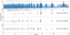 |
Fig. 26. Same unpublished data as Fig. 24, now showing the period vs fitted semi-major axis, illustrating that the observed semi-major axes typically lie between 0.1 and 10 mas (top panel), and showing that the orbital solutions fitted to the noiseless sampled bias model with amplitude 1 mas induce semi-major axes of one to several milliarcseconds (following panels). |
Lastly, we similarly verified the significance of the solution by plotting the distribution of the significance of the semi-major axes in Fig. 27. The top panel shows that a large fraction of the orbits is rather significant. This is also predicted by the simulations that are shown in the following panels (purple data).
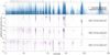 |
Fig. 27. Same unpublished data as Fig. 24, now showing the period vs fitted semi-major axis significance, illustrating the highly significant nature of most of the observed orbits (top panel), and even more so for the orbital solutions fitted to the noiseless sampled bias model with amplitude 1 mas (following panels). |
Just as for the photometric data, all these analyses seem to suggest that the vast majority of observed astrometric spurious orbital periods is due to close pairs with a fixed position angle on the sky. Although our astrometric simulations appear to be consistent with the data, we would like to caution that the high degrees of freedom of the fitted orbital model and our simplified analyses of each harmonic separately might have led to perhaps (partially) biased predictions. More in-depth analyses of the impact of astrometric bias signals on astrometric (orbital) modelling is beyond the scope of this paper, but is foreseen to be studied for Gaia DR4.
Because the offset c0 does matter in astrometry, we also ran a simulation (not shown) in which we set the offset to 1 mas, that is, c0 = 1, and the scan-angle dependent part to zero, that is, ak = 0 for all k. This effectively traces out a circle on the sky and always results in orbits with a period of 1 yr with an extremely high orbital significance (> 106) and eccentricity of about 0.033. This is twice that of the Earth’s orbit (which is 0.0167).
6. Detection of scan-angle-dependent signal
With the knowledge that potential scan-angle-dependent signals might affect the time series of some sources, the obvious question arises how they might be identified. Because photometric time series are available for a large sample of sources in Gaia DR3, we provide here several photometric diagnostics, and if they are not yet available in the Gaia DR3 archive, we publish them in a special archive table (see Appendix A) for all sources with available photometric time series. Because scan-angle-dependent signals also exist in astrometric and radial velocity time series, we are developing related diagnostics for these data that will be used in Gaia DR4 processing.
In this section, we first introduce two (partially complementary) correlation statistics: ripd described in Sect. 6.1, and rexf described in Sect. 6.2. Next we discuss the use of the small-separation binary model (Eq. (5)) described in Sect. 6.3, and finally, we describe the (combined) use of available IPD and other parameters in Sect. 6.4.
We demonstrate the distribution of these statistics for real Gaia data using the GAPS data set in Fig. 28.
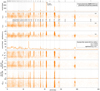 |
Fig. 28. Distribution of sources published in GAPS. The top panel shows the same data as in the second panel of Fig. 16. The following panels illustrate the distributions of various statistics that can be used to diagnose possible scan-angle-dependent signals; see text for details. An example filter has been created to show the effect on the period distribution. The total source counts are only for the period range of 10−500 d. |
6.1. Correlation with IPD model: ripd
The IPD GoF model Mipd(ψ) of Eq. (1) gives us information about the phase (and amplitude) of a potential scan-angle-dependent signal. In order to quantify how much the G, GBP, GRP is really affected by a scan-angle-dependent signal, we computed the IPD correlation: ripd. This is the Spearman correlation between a specific time series (for example G in magnitude) and the IPD GoF model sampled at the scan angles of the time-series observations:
 (8)
(8)
with i being the observation index in the time series of a source with a total of N observations, and ψi the associated scan angle. The Spearman correlation is rank based, that is, it is insensitive to the specific magnitude differences of the values and only measures the level of correlated increase or decrease between the two input time series. This means that we do not need to normalise our values, and it makes the statistic also rather robust against (small numbers of) outliers. For example, if both time series fully coherently increase and decrease as a function of scan angle, then ripd = 1, and −1 if the behaviour is inverted (that is, when one increases when the other decreases, or vice versa). This property means that ripd will be close to 1 if the signal has a scan-angle period of π like the Mipd(ψi), and is phase-coherent with the ipd_gof_harmonic_phase (the amplitude does not have any effect), as can be seen in various examples provided in Sect. 3.1. We introduced the sign 𝒮 to ensure that the correlation always gives the same value, independent of the units of the photometric input data.
Because the nominal scanning law means that scan angles do not vary smoothly between source observations separated by more than about four days (see Sect. 2.1), varying time series that do not have a scan-angle-dependent signal will create an irregular signal when ordered by scan angle and thus will have an ripd close to zero. This is even more true for data of a constant source with randomly fluctuating noise.
The table published with this paper (Appendix A) contains the IPD correlation computed for all available photometric time series with respect to G, GBP, and GRP, resulting in ripd, G, ripd, BP, and ripd, RP. Observations during the ecliptic-pole scanning law (BJD–2455197.5 < 1693.14) and those rejected by the variability analyses (variability_flag_g_reject = true in the epoch photometry) were excluded from the computation. The resulting number of observations is listed in NnoEpsl, G/BP/RP. Suggestions for minimum values for secure analyses are discussed in Appendix A. The clear correspondence of high ripd, G with the location of the spurious period peaks in the GAPS data is illustrated in Fig. 28.
A rather in-depth analyses of ripd, G on the published Gaia DR3 eclipsing binary candidates has been provided in Mowlavi et al. (2023), though no sources were filtered based on this statistic. Source filtering based on ripd, G was applied to several Gaia DR3 variability products as described in Distefano et al. (2023), Carnerero et al. (2023), and Lebzelter et al. (2023).
For completeness, we would like to point out that the correlation can be computed by the user from public data. Although the photometry is readily available, obtaining the scan angle for each observation needs more work. To do this, the particular FoV of the observations first needs to be known, which can be extracted from the transit_id3 in the epoch photometry. With the FoV, the scan angle at the time of the observation can be looked up in the commanded_scan_law4. Since this is a rather complex procedure to implement, we decided to simply pre-compute and provide these for all sources with public time series. To be precise, we used the commanded scanning law for our computations. Although this will differ slightly from the actual law, this difference is negligible for the required precision on the scan angle.
6.2. Correlation with the corrected excess flux factor: rexf
To adequately filter spurious (periods of) solar-like variable sources, Distefano et al. (2023) developed a correlation statistic based on the Spearman correlation between the G-band magnitude and corrected excess flux C*,
 (9)
(9)
using the corrected excess flux C* from Riello et al. (2021),
 (10)
(10)
where C = (IBP + IRP)/IG is the excess flux factor, IBP, IRP, and IG are the cumulative fluxes in the GBP, GRP, and G bands, and f(GBP − GRP) is the correction function defined in Table 2 of Riello et al. (2021). Observations rejected by the variability analyses (variability_flag_g_reject = true in the epoch photometry) were omitted. Because C* requires that the transit flux from all three bands is available, the resulting number of observations N3band used in the rexf correlations can occasionally be quite low (suggestions for minimum values for secure analyses are discussed in Appendix A). Sources without excess flux will have a G-band correlation rexf, G of about zero. In Sect. 3.2 and the associated Fig. 12, we report some source examples with close to zero, close to 1, and close to −1 rexf correlations for the different photometric bands. For completeness, the table published with this paper (Appendix A) contains the excess flux correlation computed for all available photometric time series with respect to G, GBP, and GRP, resulting in rexf, G, rexf, BP, and rexf, RP.
As discussed in Distefano et al. (2023), rexf, G and ripd, G are partially sensitive to the same scan-angle-dependent signals, which can also be seen from Fig. A.2, although rexf, G is also sensitive to anomalies in sources with multiple window-gate configurations and to sources with strong emission lines whose intensity is correlated with G. The clear correspondence of high rexf, G with the location of the spurious period peaks in the GAPS data is illustrated in Fig. 28.
6.3. Small-separation binary model fit diagnostics
As we showed in Sect. 5, the simple small-separation binary model (Eq. (5)) appears to be able to represent the bulk of the spurious signals observed in the Gaia data, as was illustrated in Figs. 22 and 23 in the k = 2 panels. We include the weighted fit of this model for all sources with photometric time series for all three bands G, GBP, and GRP in the table published with this paper (Appendix A). A model fit like this will be implemented in Gaia DR4 for all sources, just like the IPD parameters such as ipd_gof_harmonic_amplitude that are currently available in Gaia DR3.
For the majority of sources (that do not have any scan-angle-dependent signal), the fit will be rather poor, which is reflected in a high  , as shown in Fig. A.3. For a small subset, the
  is rather good, for instance, lower than 9, indicating that this signal is well represented by the model. However, this will also be the case for constant stars (presumably producing uncorrelated noisy observations around their mean magnitude). Therefore, either an additional threshold should be set on the fitted amplitude, or it should be combined with other statistics, as we discuss in the next section.
Figure A.5 shows the distribution of the fitted photometric model amplitude aG as function of median G magnitude. The right panel basically traces the magnitude noise-floor because most of the sources in GAPS are (almost) constant. The variable stars (left panel) cause the fitted amplitude to be inflated over a wider range, but a clear cluster with amplitudes between 0.2−0.4 mag (horizontal white lines) still stands out. That this region is related to sources with high scan-angle-dependent signals is seen in the top left inset image, which shows the same area, but now colour-coded with the median ripd, G between 0 (blue) and 1 (red), clearly highlighting the area above 0.2 mag for variable stars, and starting around 0.1 mag for the GAPS data. The second inset image shows the same colour-coding for rexf, G, clearly showing additionally regions with gate transitions at brighter magnitudes. From this figure it is clear that any cuts to aG alone should be applied with great care. For example, a fixed cut at 0.01 mag, would remove a fraction of genuine variable sources that are fainter than G-band magnitude ∼13 (as seen in the left panel), and basically all non-variable sources fainter than magnitude 19 (as seen in the right panel).
A better selection criterion seems to be the significance of aG, which is computed from the (Eq. (5)) fitted c2 and s2 and their correlation by means of Eqs. (2) and (3) of Halbwachs et al. (2023). Figures 28 and A.4 illustrate how well this statistic separates specific period peaks and how well it correlates with high values of ripd, G and rexf, G.
For sources without public time series, no fitted photometric amplitude is available, but as shown in Fig. A.6, it is strongly correlated with ipd_gof_harmonic_amplitude. The latter could therefore be used (for ipd_gof_harmonic_amplitude ≳ 0.07) as a lower-quality fall-back estimate of the photometric amplitude.
Finally, we note that we used the same selection for the observations as in Sect. 6.1, that is, we rejected outliers and excluded the period with the ecliptic poles scanning law (EPSL).
6.4. Combining different indicators
When the Gaia DR3 catalogue is used as-is, we can make use of some of the indicators previously described in Sect. 3.1.2. Statistics ipd_frac_multi_peak and ipd_gof_harmonic_amplitude seem to be the most useful indicators. The type of AGIS solution (two-parameters versus five- or six-parameters) can also indicate that the source is problematic. In general, these features can be used to apply some filters such as those listed below (a summary of the main filters can be found in Fig. 29).
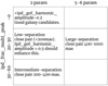 |
Fig. 29. Parameter domain map for the filters based on the main source statistics. |
– Sources with a moderate value in ipd_frac_multi_peak (for example 20 to 30) and a two-parameter astrometric solution even though enough transits are matched (that is, astrometric_params_solved = 3 and matched_transits of about 30 or more) are good candidates to be a low-separation close pair, probably below 200 mas. High values in ipd_gof_harmonic_amplitude (for example 0.5 and above) should enhance this.
– Sources with the same conditions, but a quite higher ipd_frac_multi_peak value (for example 30 to 60) should also be good close pair candidates, but this time, with a higher separation, such as 200 to 400 mas.
– Sources with a five- or six-parameter astrometric solution and moderate ipd_frac_multi_peak (for example 20 to 30) should be close pairs with higher separations, such as 400 to 1000 mas.
– In addition to these conditions, we can also check for ipd_frac_odd_win: moderate and high values (for example 20 and above) should select the weaker sources of the pairs, typically corresponding to the fainter components of the pairs, which are more strongly truncated in their windows. In contrast, low values should select the stronger sources, in which the IPD may have detected (and masked) the secondary peaks.
– When we select sources with a moderate ipd_gof_harmonic_amplitude (for example 0.2 and above) and an ipd_frac_multi_peak value of zero or nearly zero, we should find good galaxy candidates with a relatively high ellipticity. Sources with two-parameter astrometric solutions and a high number of transits (for example 30 or more) should enhance this.
In addition to these built-in features, the new indicators rexf, G and ripd, G provide even more reliable indications of scan-angle-dependent signals. Remarkably, the correlation with a corrected excess flux factor rexf, G for the G band exhibits values typically above 0.4 for close pairs, with values approaching 1.0 for very small separations. The correlation with IPD model ripd, G seems to be more useful for extended sources (where rexf, G just shows moderate values), although it also exhibits high values in many cases of close pairs.
Combining a high ripd, G (for example > 0.8) with a low  (for example < 9) potentially is a good way to select a sample of highly affected sources with a sinusoidal scan-angle-dependent signal, as shown in Fig. A.3. Many sources without particular variability easily produce a low
  when the fitted amplitude is basically set to a very low value. This criterion should therefore only be used in combination with other indicators. A better single-parameter alternative probably is the significance of aG, which we discussed in the previous section.
As must be clear from this section, there are a variety of ways to identify potential scan-angle-dependent signals. Although some are more powerful than others, it is difficult to provide a clear recipe of how to use them as this is highly dependent on (1) the sky location, (2) the use case at hand (see also the discussion in Sect. 7.5), and (3) the purity or contamination that is sought. To obtain an impression of how these indicators influence the period peaks, we refer to the visual overview in Fig. 28, which shows the distribution of the main diagnostics discussed in this section for the public GAPS data for which we provide all parameters in Appendix A. It also demonstrates a potential filter combining ripd, G, rexf, G and the significance of aG, which removes, or at least largely decreases, the spurious peaks.
7. Discussion
This section is meant to provide both a compact synthesis of this paper and answer some specific questions that may have arisen. It is to serve as a guide to available and planned developments.
7.1. Scan-angle-dependent signals in a nutshell
In Sect. 3 and Appendix B, we discuss that the Gaia instrument data reduction can introduce modelling errors (referred to as scan-angle-dependent signals) when on-sky source structure is present. This structure can be interpreted in a very broad way, covering: (1) multiple close-pair (≲1″) sources of a point-like nature; (2) extended or non-symmetric sources (for example cores of galaxies or tidally distorted stars); (3) sources with a (much) brighter neighbour close by (> 1″); and (4) combinations of any of the above. In principle, the structure can either be static, like a galaxy core or very long-period binaries (P ≫ 5 y), or dynamic, like a short-term orbital binary.
Subsequently, there are constraints on the data acquisition of sources by the Gaia instruments: (1) observations consist of pixel values extracted in a limited window around each source; (2) observations are made with a large variety of on-sky scan angles due to the scanning law of the spacecraft (Sect. 2); (3) pixels have an aspect ratio of roughly 1:3, the highest resolution of which is in the along-scan direction, that is, along the scan angle; and (4) for sources with G ≥ 13, all the data in the across-scan direction are collapsed into one-dimensional along-scan pixel counts, which enhances the effect of scan-angle-dependent signals.
The combined effect of structure, data acquisition, and the challenge of processing these data can cause scan-angle-dependent signals to appear in derived time-series values of Gaia DR3. In this paper, we abundantly demonstrate this to be the case in publicly available photometric G-band time series, but it equally exists in the (unpublished) astrometry and radial velocity time series (see Table 1 for examples).
7.2. Spurious periods in a nutshell
Examples of observed distributions of pre-cleaned spurious period peaks are shown in Sect. 4. To understand the emergence of spurious peaks caused by scan-angle-dependent signals, we need to first realise that the scan angle associated with each observation of the time series of a source is dictated by the scanning law, as explained in Sect. 2. Depending on the ecliptic position (mainly latitude) of a source, it causes different resonances in the data (Eq. (3)) that are related to harmonics of the ∼63 day spin-axis precession period and the one-year orbital period around the Sun. In Sect. 5.4 we demonstrate using simulations that we can indeed qualitatively reproduce the structure of spurious period peaks in both photometry and astrometry by propagating scan-angle-dependent bias signals. For examples of public photometry that are phase folded with their spurious period, see Appendix C.
7.3. Photometric amplitude of scan-angle-dependent signals
In Sect. 5 we introduced two models for the scan-angle signal in the G-band photometry for a close binary. The model of Eq. (4) provides a prediction of the expected amplitudes based on various parameters such as the magnitude difference, while the model of Eq. (5) is only accurate for small binary separations. The simplicity of the latter model allows it to be easily fitted to all time series and thus has been provided for the three photometric bands of all sources with published time series in Appendix A. We can use the latter fitted model parameters for sources that show a strong indication of scan-angle-dependent signals to form an idea of the amplitude of the photometric effect. From the published data, we find aG amplitudes of 0.2 − 0.4 mag for sources with G ≳ 16, as shown in Fig. A.5. From internal tests on pre-filtered data (not shown), we find that amplitudes can range even wider: from 0.05 − 0.5 mag down to G ∼ 13; the scan-angle-dependent signal for brighter magnitudes is generally weaker (but not absent; see Fig. B.2 as an example) due to the availability of two-dimensional window data.
For sources without public time series, the rather strong relation between ipd_gof_harmonic_amplitude and G photometric scan-angle model amplitude (aG) for ipd_gof_harmonic_amplitude ≳ 0.07 can also be used, as shown in Fig. A.6. This allows estimating the latter G scan-angle-dependent amplitude in magnitudes by the value of ipd_gof_harmonic_amplitude (see Sect. 6.3 for more details).
7.4. Work with scan-angle-dependent signals
As shown, multiple and extended sources can lead to scan-angle-dependent signals that can incorrectly be identified as astrophysical features of single point-like sources. The most typical example is the spurious detection of photometric variability, but we can also obtain spurious solutions of non-single stars, spurious extragalactic features, or other types of an incorrect astrophysical parameter determination. Despite the exhaustive validation made in DPAC, some of these spurious solutions may still exist, as illustrated in this paper. Fortunately, the several quality, multiplicity, and scan-angle-dependence indicators discussed in Sect. 6 (and Sect. 3.1.2) in many cases help to identify them.
7.5. Rejection of affected sources from a study
First, a possible rejection depends importantly on which parameters from the Gaia data are used. Especially when a period derived from Gaia data or other parameters is to be used that depends on the (phase-folded) shape of the time-series signal, we recommend to avoid sources that are affected in any significant way by using the statistics discussed in Sect. 6.
If this information is not needed, it needs to be determined whether the targets might exhibit some source structure (see definition Sect. 7.1) that might produce a scan-angle-dependent signal. When the targets have no source structure, then we again recommend to avoid sources that appear to be affected by scan-angle-dependent signals (at the cost of some loss of completeness due to imperfect filtering statistics) because otherwise, they might cause contaminate the sample.
When the targets have some source structure, then it becomes more delicate, as scan-angle-dependent signals might be expected to appear. For example, when binaries with long orbital periods are to be identified, we can expect a strong scan-angle-dependent signal (and potentially a Gaia periodicity at one of the spurious peaks). If the purpose is to identify these binaries, then this signal might be used as valid selection criterion. However, it must then be verified that the source is in a non-dense environment and has no nearby bright stars (that is, the signal is not caused by background or nearby polluting stars or PSF spike pollution).
7.6. Modelling the source environment around Gaia sources
Following the discussion in Sect. 3.1.1 related to the difficulty of extracting source information from a window that contains more than a single point-source, it might be wondered whether the source environment might be derived around all Gaia stars.
Starting from the fact that the AL-scan pixel size of Gaia is about 59 mas, this means that Hubble-like resolution knowledge of the environment around each of the billion stars would be obtained. Although Gaia observations can certainly be affected by sources ≥1 arcsec away (meaning ground-based priors could certainly have their merit here), many of the complications related to close-binaries affect the 0.1−1.0 arcsec regime.
It is too computer intensive to do at the IPD level, but all available two- and one-dimensional Gaia observations of a source taken under a variety of scan angles can be used to try and reconstruct its environment. This is exactly the goal of two specific work-packages in Gaia: (1) The CU4-EO surface brightness profile-fitting pipeline, which is dedicated to deriving the morphological parameters of galaxies observed by Gaia (see Ducourant et al. 2023; Gaia Collaboration 2023b), the results of which are published in the DR3 galaxy archive table, and (2) the source environment analysis pipeline (SEAPipe). The aim of SEAPipe is to combine the transit data for each source and to identify any additional sources in the local vicinity. The first operation in SEAPipe is image reconstruction, where a two-dimensional image is formed from the mostly one-dimensional transit data (G > 13 mag). The algorithm used to perform the image reconstructions is described in Harrison (2011). These images are then analysed and classified, based on whether the source is extended, whether additional sources are present, or whether the source is an isolated point source within the reconstructed image area (radius of ∼2″). The full SEAPipe analysis will be described in Harrison et al. (in prep.) and is planned to be included in Gaia DR4.
As mentioned in Sect. 3.1.1, none of these methods will be used in the IPD centroid or flux estimation. However, they can nonetheless be used for a post-Gaia re-analysis of the window data accounting for (some) of the source structure and environment, together with publicly available large-scale imaging survey data. This will allow improving the amount and accuracy of the information that can be extracted. Through the improved modelling, this might then also lead to the disappearance of scan-angle-dependent signals in the derived photometric and astrometric time series data. It seems likely that this might be beneficial for the subset of sources that were identified to be particularly non-point-like in the DPAC Gaia analyses.
7.7. Fitting and resolving multiple peaks in IDU
As shown in Sect. 3.1.2, IDU determines some quality and multiplicity indicators in the IPD, which are then combined at a source level by AGIS and later published in DR3. The ipd_frac_multi_peak relies on the detection of additional peaks in the window, as explained previously. The next desirable step would be to fit the multiple peaks found in the window (instead of just masking them, as in DR3), determining one set of image parameters per detected peak. This detection and fit could take advantage of the several AF windows available per scan, aligning them using the instrumental calibration, and a combined processing might be performed. With this, the signal-to-noise ratio would be better and the PSF or LSF subsampling would be mitigated, enhancing the secondary peaks and allowing for a better fit. With this approach, we would also achieve intra-scan consistency, that is, we would obtain consistent IPD results for each of the peaks throughout the several AF windows in each scan, avoiding swaps between the peaks. However, inter-scan consistency would also be required. This means that we need to ensure that the peaks corresponding to the same astrophysical source from all scans are consistently matched, avoiding swaps between peaks and sources. This would require quite complex cross-matching and clustering algorithms. Peak detections from one-dimensional windows would require an adequate handling of their large uncertainty in the across-scan direction.
This approach has already been implemented and executed in IDU in preparation for DR4, with very good results. The first example shown in Sect. 3.1.3 (Fig. 7) corresponds to a real, low-separation close pair that is correctly resolved with this approach. While the overall resolution for these cases has vastly improved in terms of new catalogue entries and astrometric solution, we are still evaluating the scan-angle dependence of their IPD GoF, and that of their epoch photometry when available.
7.8. Co-modelling the scan-angle-dependent signal
When it is known that time series might contain scan-angle-dependent signals, as in Gaia DR3, the most desirable option is to co-model the disturbing scan-angle signal in addition to the source signal that is searched for, for instance, following the concept of partial distance correlation presented in Binnenfeld et al. (2022). For photometry, the nuisance model could be parametrised as in Eq. (4), or to first order as in Eq. (5). This is different from the G model fit provided in Appendix A, which only fits Eq. (5) and does not fit for any source model.
8. Conclusions
We have presented an overview of the origin and background of scan-angle-dependent signals in the Gaia DR3 data for the different instruments, which are generally caused by non-point-like object structure (mainly multiplicity or extendedness) or contamination from nearby (brighter) stars. We qualitatively demonstrated that specific spurious periodic signals can be propagated into the photometric and astrometric time series when a dominating scan-angle-dependent signal is present at the right phase given the sky-position-dependent observation sampling; not all scan-angle-dependent signals therefore cause spurious periods. We would like to caution that the reverse is also true: not all features at the location of spurious periods are due to scan-angle-dependent signals, as these frequencies are specifically connected to regularities in the NSL that dictate the sampling and window function of the observations of each source. For example, BH-1, the first nearby black hole companion discovered in Gaia DR3 data (El-Badry et al. 2023; Chakrabarti et al. 2022), falls directly into a spurious period range with its 186 d orbital period and was therefore not mentioned in Gaia Collaboration (2023a).
This does not detract from our conclusion that the majority of spurious period peaks is caused by scan-angle-dependent signals originating from fixed-orientation optical pairs with a separation of < 0.5″ (including binaries with P ≫ 5 y) and (cores of) distant galaxies, as they are already well reproduced with our simple models.
For the sample of sources with published epoch photometry in Gaia DR3, several statistics are published with this paper to help identify sources that might be affected, and thus reveal information of sub-arcsecond scale structure, especially in terms of binarity.
Although the vast majority of sources that are affected by these signals have been filtered out of the Gaia DR3 archive nss_two_body_orbit and several vari tables, a certain fraction remains. Its existence should therefore be acknowledged (no sources were filtered from gaia_source). Improved modelling in the data processing will likely reduce the effect in future data releases.
See Gaia archive documentation for ipd_gof_harmonic_phase.
See transit_id in Sect. 20.7.1 of van Leeuwen et al. (2022).
See commanded_scan_law, Sect. 20.3.1 van Leeuwen et al. (2022).
Acknowledgments
We thank the anonymous referee and Floor van Leeuwen for their detailed feedback and suggestions that improved this paper. This work has, in part, been carried out within the framework of the National Centre for Competence in Research PlanetS supported by SNSF. This work presents results from the European Space Agency (ESA) space mission Gaia. Gaia data are being processed by the Gaia Data Processing and Analysis Consortium (DPAC). Funding for the DPAC is provided by national institutions, in particular the institutions participating in the Gaia MultiLateral Agreement (MLA). The Gaia mission website is https://www.cosmos.esa.int/gaia. The Gaia archive website is https://archives.esac.esa.int/gaia. Full acknowledgements are given in Appendix E. This work made use of software from Java (https://www.oracle.com/java/), POSTGRES-XL (https://www.postgres-xl.org), TBase database management system (https://github.com/Tencent/TBase), DATAGRAPH (https://www.visualdatatools.com/DataGraph/), TOPCAT (https://www.star.bris.ac.uk/~mbt/topcat/), (Taylor 2005), GNUPLOT (http://www.gnuplot.info), and MATLAB (https://www.mathworks.com/products/matlab.html).
References
- Alcock, C., Allsman, R., Alves, D. R., et al. 2000, ApJ, 542, 257 [NASA ADS] [CrossRef] [Google Scholar]
- Baluev, R. V. 2009, MNRAS, 395, 1541 [CrossRef] [Google Scholar]
- Binnenfeld, A., Shahaf, S., Anderson, R. I., & Zucker, S. 2022, A&A, 659, A189 [NASA ADS] [CrossRef] [EDP Sciences] [Google Scholar]
- Bonett, D. G., & Wright, T. A. 2000, Psychometrika, 65, 23 [CrossRef] [Google Scholar]
- Boubert, D., Strader, J., Aguado, D., et al. 2019, MNRAS, 486, 2618 [Google Scholar]
- Carnerero, M. I., Raiteri, C. M., Rimoldini, L., et al. 2023, A&A, 674, A24 (Gaia DR3 SI) [NASA ADS] [CrossRef] [EDP Sciences] [Google Scholar]
- Castañeda, J., Hobbs, D., Fabricius, C., et al. 2022, Gaia DR3 Documentation Chapter 3: Pre-processing, Gaia DR3 Documentation, European Space Agency; Gaia Data Processing and Analysis Consortium, 3. Online at https://gea.esac.esa.int/archive/documentation/GDR3/index.html [Google Scholar]
- Chakrabarti, S., Simon, J. D., Craig, P. A., et al. 2022, AAS, submitted, [arXiv:2210.05003] [Google Scholar]
- Clementini, G., Ripepi, V., Molinaro, R., et al. 2019, A&A, 622, A60 [NASA ADS] [CrossRef] [EDP Sciences] [Google Scholar]
- Cropper, M., Katz, D., Sartoretti, P., et al. 2018, A&A, 616, A5 [NASA ADS] [CrossRef] [EDP Sciences] [Google Scholar]
- Cumming, A., Marcy, G. W., & Butler, R. P. 1999, ApJ, 526, 890 [Google Scholar]
- de Bruijne, J., Siddiqui, H., Lammers, U., et al. 2010, in Relativity in Fundamental Astronomy: Dynamics, Reference Frames, and Data Analysis, eds. S. A. Klioner, P. K. Seidelmann, & M. H. Soffel, 261, 331 [NASA ADS] [Google Scholar]
- de Bruijne, J., Babusiaux, C., Brown, A., et al. 2022, Gaia DR3 Documentation Chapter 1: Introduction, Gaia DR3 documentation, European Space Agency; Gaia Data Processing and Analysis Consortium, 1. Online at https://gea.esac.esa.int/archive/documentation/GDR3/index.html [Google Scholar]
- Distefano, E., Lanzafame, A. C., Brugaletta, E., et al. 2023, A&A, 674, A20 (Gaia DR3 SI) [NASA ADS] [CrossRef] [EDP Sciences] [Google Scholar]
- Ducourant, C., Krone-Martins, A., Galluccio, L., et al. 2023, A&A, 674, A11 (Gaia DR3 SI) [NASA ADS] [CrossRef] [EDP Sciences] [Google Scholar]
- Duquennoy, A., & Mayor, M. 1991, A&A, 248, 485 [NASA ADS] [Google Scholar]
- El-Badry, K., Rix, H.-W., Quataert, E., et al. 2023, MNRAS, 518, 1057 [Google Scholar]
- Evans, D. W., Eyer, L., Busso, G., et al. 2023, A&A, 674, A4 (Gaia DR3 SI) [NASA ADS] [CrossRef] [EDP Sciences] [Google Scholar]
- Eyer, L., Mowlavi, N., Evans, D. W., et al. 2017, ArXiv e-prints [arXiv:1702.03295] [Google Scholar]
- Eyer, L., Audard, M., Holl, B., et al. 2023, A&A, 674, A13 (Gaia DR3 SI) [NASA ADS] [CrossRef] [EDP Sciences] [Google Scholar]
- Fabricius, C., Bastian, U., Portell, J., et al. 2016, A&A, 595, A3 [NASA ADS] [CrossRef] [EDP Sciences] [Google Scholar]
- Fabricius, C., Luri, X., Arenou, F., et al. 2021, A&A, 649, A5 [NASA ADS] [CrossRef] [EDP Sciences] [Google Scholar]
- Gaia Collaboration (Prusti, T., et al.) 2016, A&A, 595, A1 [NASA ADS] [CrossRef] [EDP Sciences] [Google Scholar]
- Gaia Collaboration (Arenou, F., et al.) 2023a, A&A, 674, A34 (Gaia DR3 SI) [CrossRef] [EDP Sciences] [Google Scholar]
- Gaia Collaboration (Bailer-Jones, C. A. L., et al.) 2023b, A&A, 674, A41 (Gaia DR3 SI) [NASA ADS] [CrossRef] [EDP Sciences] [Google Scholar]
- Garcez de Oliveira Krone Martins, A. 2011, PhD Thesis, University of São Paulo, Brazil and University of Bordeaux, France [Google Scholar]
- Górski, K. M., Banday, A. J., Hivon, E., & Wandelt, B. D. 2002, ASP Conf. Ser., 281, 107 [Google Scholar]
- Halbwachs, J.-L., Pourbaix, D., Arenou, F., et al. 2023, A&A, 674, A9 (Gaia DR3 SI) [NASA ADS] [CrossRef] [EDP Sciences] [Google Scholar]
- Harrison, D. L. 2011, Exp. Astron., 31, 157 [NASA ADS] [CrossRef] [Google Scholar]
- Heck, A., Manfroid, J., & Mersch, G. 1985, A&AS, 59, 63 [NASA ADS] [Google Scholar]
- Holl, B., Lindegren, L., & Hobbs, D. 2012, A&A, 543, A15 [NASA ADS] [CrossRef] [EDP Sciences] [Google Scholar]
- Holl, B., Sozzetti, A., Sahlmann, J., et al. 2023, A&A, 674, A10 (Gaia DR3 SI) [NASA ADS] [CrossRef] [EDP Sciences] [Google Scholar]
- Katz, D., Sartoretti, P., Guerrier, A., et al. 2023, A&A, 674, A5 (Gaia DR3 SI) [NASA ADS] [CrossRef] [EDP Sciences] [Google Scholar]
- Kovács, G., Zucker, S., & Mazeh, T. 2002, A&A, 391, 369 [Google Scholar]
- Lebzelter, T., Mowlavi, N., Lecoeur-Taibi, I., et al. 2023, A&A, 674, A15 (Gaia DR3 SI) [NASA ADS] [CrossRef] [EDP Sciences] [Google Scholar]
- Lindegren, L. 2022, Gaia Data Processing and Analysis Consortium (DPAC), Technical Note GAIA-C3-TN-LU-LL-136, http://www.cosmos.esa.int/web/gaia/public-dpac-documents [Google Scholar]
- Lindegren, L., & Bastian, U. 2010, EAS Publ. Ser., 45, 109 [NASA ADS] [CrossRef] [EDP Sciences] [Google Scholar]
- Lindegren, L., Lammers, U., Hobbs, D., et al. 2012, A&A, 538, A78 [NASA ADS] [CrossRef] [EDP Sciences] [Google Scholar]
- Lindegren, L., Klioner, S. A., Hernández, J., et al. 2021, A&A, 649, A2 [EDP Sciences] [Google Scholar]
- Mowlavi, N., Holl, B., Lecœur-Taïbi, I., et al. 2023, A&A, 674, A16 (Gaia DR3 SI) [NASA ADS] [CrossRef] [EDP Sciences] [Google Scholar]
- Paturel, G., Petit, C., Prugniel, P., et al. 2003, A&A, 412, 45 [NASA ADS] [CrossRef] [EDP Sciences] [Google Scholar]
- Penoyre, Z., Belokurov, V., & Evans, N. W. 2022, MNRAS, 513, 2437 [NASA ADS] [CrossRef] [Google Scholar]
- Riello, M., De Angeli, F., Evans, D. W., et al. 2021, A&A, 649, A3 [NASA ADS] [CrossRef] [EDP Sciences] [Google Scholar]
- Rowell, N., Davidson, M., Lindegren, L., et al. 2021, A&A, 649, A11 [EDP Sciences] [Google Scholar]
- Sartoretti, P., Katz, D., Cropper, M., et al. 2018, A&A, 616, A6 [NASA ADS] [CrossRef] [EDP Sciences] [Google Scholar]
- Seabroke, G. M., Fabricius, C., Teyssier, D., et al. 2021, A&A, 653, A160 [NASA ADS] [CrossRef] [EDP Sciences] [Google Scholar]
- Taylor, M. B. 2005, ASP Conf. Ser., 347, 29 [Google Scholar]
- van Leeuwen, F. 2007, Hipparcos, the New Reduction of the Raw Data: Astrophysics and Space Science Library (Springer Science+Business Media B.V.), 350 [CrossRef] [Google Scholar]
- van Leeuwen, F., de Bruijne, J., Babusiaux, C., et al. 2022, Gaia DR3 Documentation, Gaia DR3 Documentation, European Space Agency; Gaia Data Processing and Analysis Consortium, 1. Online at https://gea.esac.esa.int/archive/documentation/GDR3/index.html [Google Scholar]
- Zechmeister, M., & Kürster, M. 2009, A&A, 496, 577 [CrossRef] [EDP Sciences] [Google Scholar]
- Zucker, S., & Mazeh, T. 1994, ApJ, 420, 806 [NASA ADS] [CrossRef] [Google Scholar]
Appendix A: Gaia archive table with photometric correlation coefficients and a small-separation binary model fit for all sources with published time series
As part of this paper, the table vari_spurious_signals is published in the Gaia DR3 archive for all 11 754 237 sources with published photometric time series, that is, for sources in gaia_source with has_epoch_photometry=true. Of these, 10 509 536 sources are variables (Eyer et al. 2023) and 1 257 319 are part of GAPS (Evans et al. 2023). They can be identified in gaia_source by their phot_variable_flag=VARIABLE and in_andromeda_survey=true flags, respectively. We note that 12 618 sources overlap between the two.
This table contains the parameters listed in Table A.1 (see also the Gaia archive documentation5): the ripd and rexf correlations for the three photometric bands along with the available number of observations for each, as introduced in Sect. 6. Additionally, for the G-band photometry, it contains a fit to the small-separation binary model introduced in Sect. 5. When fewer than six observations were available for the computation of a value, we found it to be generally unusable and set the value to be missing (null). However, we caution that (much) more stringent cuts need to be applied on the number of observations for different parameter values. As illustrated in Fig. A.1, the rexf and ripd are not really meaningful for fewer than 11 points, and some biases and features disappear only above 20 or 30. This is related to the fact that for the Gaia DR3 34 months of data, the scanning law should have provided sources all over the sky with at least 15–20 observations, and sources with fewer observations are generally found in crowded regions and/or are at the faint end, which makes them more susceptible to disturbances and/or non-detections. This increase in (scan-angle-dependent) disturbances is illustrated by the rise in G-band correlations towards fewer observations. In the heat maps, we normalised the values for each number of observation bin to highlight the change in spread in the correlation distribution. True source-count distributions are provided by the histograms above and on the side of the heat maps. For a more detailed discussion of the relation between the number of points and the significance of the Spearman correlation, see for example Bonett & Wright (2000). The general increase in spread in all correlations towards fewer observations illustrates this relation.
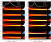 |
Fig. A.1. Correlations based on the published photometric time series in Gaia DR3. Top panels: Histograms of the number of available observations for the different correlation coefficients. Second to fourth panel rows: ipd correlation coefficients (Sect. 6.1). Fifth to seventh panel rows: Corrected excess factor correlation coefficients (Sect. 6.2). On the right side, a histogram illustrates the distribution of each correlation coefficient. The left panels contain the values for the 10.5 million variables, and the right panels show the values for the 1.3 million sources in GAPS. The heat maps are value normalised per number of observation bin to highlight the level of parameter spread. The histograms on the right sides represent the true count distribution for each parameter. |
gaia_dr3.vari_spurious_signalsGaia archive table fields. See the Gaia archive documentation for more detailed descriptions.
The parameters of the G-band photometry fit to the small-separation binary model of Eq. 5 (fields labelled scan_angle_model_*) are provided for all sources with six observations at least, but are only meaningful for sources with high G-band correlations, for instance rexf, G and/or ripd, G > 0.8 and with a sufficient number of observations, where we recommend num_obs_excl_epsl_g_fov to be above 20 or 30. Parameters outside of this scope can be an arbitrary poor fit to the data, as the model is simply not applicable: these values therefore have to be used with appropriate care. Additionally, from Sect. 6.3, the significance of the amplitude (*ampl_sig*) and  of the fit (*red_chi2*) are provided. Finally, we also provide the F2, or Gaussianised χ2.
For this model fit, we used the same observations as for ripd, that is, we excluded the ecliptic pole scanning law observations due to their highly clustered scan angles, which easily bias the effective weight of the fit to only a small scan-angle range. For more information about the various diagnostic parameters in this table, see Sect. 6.
For completeness, we include the generalised least-squares (“gls”) period search result frequency, amplitude, signal detection efficiency (SDE; see Alcock et al. 2000; Kovács et al. 2002), and Baluev false-alarm probability (Baluev 2009) at the beginning of the table, and the frequency and estimated error from a subsequent non-linear harmonic modelling (nhm), as was described in Sect. 4.1.
The additional Figs. A.2, A.3, A.4, A.5, and A.6 are presented here to support discussions in the body of this paper that are based on the data published with this paper.
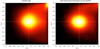 |
Fig. A.2. Density plots of the rexf, G vs ripd, G correlation with at least 20 observations for each statistic (N3band ≥ 20 and NnoEpsl, G ≥ 20). See Sect. 6 for a discussion. |
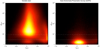 |
Fig. A.3. Density plot of the relation between ripd, G and |


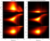 |
Fig. A.4. Density plots of various parameters in relation to the significance of aG, the amplitude of the small-separation binary model fit to the G-band photometry (Eq. 5). The white vertical line indicates a significance threshold of 6, above which the fitted amplitude is more likely due to a scan-angle-dependent signal. In the top panels, the same low |

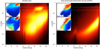 |
Fig. A.5. Density of the median G-band magnitude dependence of aG, the amplitude of the small-separation binary model fit to the G-band photometry (Eq. 5). The top left inset images shows the same data colour-coded with the median ripd, G and rexf, G, respectively, both ranging between 0 (blue) and 1 (red). See Sect. 6.3 for discussion. Plots are restricted to sources with N3band ≥ 20 and NnoEpsl, G ≥ 20. |
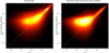 |
Fig. A.6. Density plot of the relation between ipd_gof_harmonic_amplitude and aG (the amplitude of the fit to the G-band photometry (Eq. 5). For ipd_gof_harmonic_amplitude ≳0.07, this relation is very strong (see Sects. 3.1.3, 6.3, and 7.3 for a more detailed discussion). Plots for N3band ≥ 20 and NnoEpsl, G ≥ 20. |
Appendix B: Additional examples of scan-angle-dependent signals in IPD outputs
As an extension of Sect. 3.1, the following figures show some representative examples covering different cases, such as angular separations between close pairs of sources, observations with one- and two-dimensional windows, bright nearby sources, and single sources identified (and characterised) as galaxies.
B.1. Unresolved close pairs in DR3
The first set of cases includes sources that are delivered in DR3 as single sources, but have some quality indicators or features that make them reasonable candidates to be unresolved close pairs. The following examples have been confirmed as close source pairs by IDU during the data processing for DR4.
The first example, already shown in Sect. 3.1, is taken from the outputs of query
-- ADQL query on DR3, aiming at <200mas 1D:
SELECT TOP 100 * FROM gaiadr3.gaia_source WHERE
in_andromeda_survey='TRUE'
AND phot_g_mean_mag>=14 AND phot_g_mean_mag>19
AND ipd_frac_multi_peak<30 AND ipd_frac_multi_peak>20
AND pmra IS NULL AND matched_transits>30
AND visibility_periods_used>18
AND astrometric_matched_transits > 30 ORDER BY random_index,
which corresponds to a source with just a two-parameter solution from AGIS, a very high rexf, G and ripd, G Spearman correlations (see Sect. 6), quite high IPD GoF harmonic amplitude, but a modest fraction of IPD multiple peaks. Fig. 7 shows that the epoch G magnitude strongly varies with the scan angle, whereas the GBP and GRP magnitudes both remain mostly constant. When we verified the IDU pre-DR4 data, we found that this DR3 source indeed is a close pair with a very small separation of just 130 mas, with one-dimensional windows and nearly the same magnitude in both sources. It is at the limit of the IDU on-ground detection capability of close source pairs for DR4. Figure B.1 shows another example obtained from the same query, corresponding to a close pair with a slightly larger separation of about 170 mas.
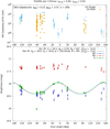 |
Fig. B.1. SourceID 388466602081536640: Scan-angle signatures. |
The next example, taken from the outputs of query
-- ADQL query on DR3, aiming at <400mas 2D:
SELECT TOP 100 * FROM gaiadr3.gaia_source WHERE
in_andromeda_survey='TRUE'
AND phot_g_mean_mag>=8 AND phot_g_mean_mag<12
AND ipd_frac_multi_peak<60 AND ipd_frac_multi_peak>30
AND pmra IS NULL AND matched_transits>30
AND visibility_periods_used>18
AND astrometric_matched_transits > 30 ORDER BY random_index,
also corresponds to a two-parameter AGIS solution, but is now bright enough to have two-dimensional windows. Again, the rexf, G and ripd, G correlations are both very high, the IPD GoF harmonic amplitude is also quite high, and the IPD multi-peak fraction is slightly higher than in the previous case, with a secondary detected (and masked) peak in basically one-third of the transits. As shown in Fig. B.2, the BP and RP magnitudes are both nearly constant again, but the G magnitude varies strongly (over 0.7 magnitudes) and is strongly correlated with the scan angle. It is worth noting that the fainter transits typically correspond to those with a secondary detected and masked peak, which means that the other peaks (in which no secondary source was detected) include unmodelled and unmitigated flux contamination. When we examined IDU pre-DR4 data, this DR3 source corresponded to a close pair with a separation of just 143 mas, a position angle of 30°, similar magnitudes, and a significant proper motion (with a very similar direction for both sources).
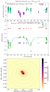 |
Fig. B.2. SourceID 378810450446502400: Scan-angle signatures and image reconstructed by SEAPipe. |
Taking the same query, we can also find Fig. B.3, with a strong and correlated G variation and very high rexf, G correlation. However, in this case, the ripd, G correlation value is lower, as is the IPD GoF harmonic amplitude, although nearly half the transits have multiple peaks. In pre-DR4 IDU, it corresponds to a close pair separated by about 350 mas, two-dimensional windows, significant proper motion (with similar vectors), and a magnitude difference of about one between them. For illustrative purposes, we also show the raw windows for some of its transits in the bottom panels of Fig. B.3. The two peaks can appear clearly separated or blended, depending on the orientation.
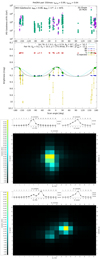 |
Fig. B.3. SourceID 385804856230839552: Scan-angle signatures (top panels) and raw windows for some of its transits (bottom panels). |
Additional examples can be found from query
-- ADQL query on DR3, aiming at 200-400mas 1D:
SELECT TOP 1000 * FROM gaiadr3.gaia_source WHERE
in_andromeda_survey='TRUE'
AND phot_g_mean_mag>=14 AND phot_g_mean_mag<19
AND ipd_frac_multi_peak>30 AND pmra IS NULL
AND matched_transits>30 AND visibility_periods_used>18
AND astrometric_matched_transits > 30 ORDER BY random_index,
which also yields a two-parameter AGIS solution, with one-dimensional windows as in the first example, but now with a higher fraction of IPD multiple peaks (nearly half the transits). The rexf, G and ripd, G correlations are very high again, as is the IPD GoF harmonic amplitude. Here, Fig. B.4 again shows the correlation with the scan angle for G, and also a number of variations in BP (although without a very clear correlation with the scan angle). Again, brighter transits correspond to those without detected secondary peaks. In IDU pre-DR4 data, this DR3 source corresponds to a close pair separated by 246 mas and feasible five-parameter astrometric solution. Because of the larger separation between the components, Eq. 4 provides a better fit and is able to reach quite good estimates for the separation and position angle. For illustrative purposes, we show two of its CCD observations in the bottom panels of Fig. B.4, similarly as in Fig. B.3, but now in one-dimensional windows. It clearly reveals the two peaks in one of the scans, and just one blended peak in another scan.
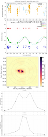 |
Fig. B.4. SourceID 382159975182923264: Scan-angle signatures, image reconstructed by SEAPipe, and two of the CCD observations taken at different scan angles. |
Further examples from the same query are shown in Fig. B.5 and Fig. B.6.
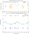 |
Fig. B.5. SourceID 376045247423005184: Scan-angle signatures. |
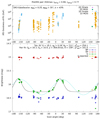 |
Fig. B.6. SourceID 385844060692409344: Scan-angle signatures. |
Finally, with the query
-- ADQL query on DR3, aiming at >400mas 1D:
SELECT TOP 1000 * FROM gaiadr3.gaia_source WHERE
in_andromeda_survey='TRUE'
AND phot_g_mean_mag>=14 AND phot_g_mean_mag<19
AND ipd_frac_multi_peak<30 AND ipd_frac_multi_peak>20
AND pmra IS NOT NULL AND matched_transits>30
AND visibility_periods_used>18
AND astrometric_matched_transits > 30 ORDER BY random_index,
we find Fig. B.7, with rather modest G variations, but it is stronger in BP and RP. The internal DR3 IDU data reveal a moderate scan-angle correlation in the epoch GoF values, although the DR3 harmonic amplitude is very small. The Spearman rexf, G and ripd, G correlations for G are rather modest, but significant. Pre-DR4 IDU data reveal a 693 mas close pair here, which is also quite nicely revealed from Eq. 4 fitting results. Yet another example from the same query is shown in Fig. B.8.
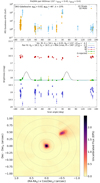 |
Fig. B.7. SourceID 385367010081173504: Scan-angle signatures and image reconstructed by SEAPipe. |
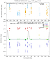 |
Fig. B.8. SourceID 387325652606842368: Scan-angle signatures. |
B.2. Resolved close pairs in DR3
The second set of examples corresponds to pairs that have been resolved as separate sources in DR3, obtained through the query plus a simplistic nearest-neighbour cross match on the result. The first example was already shown in Sect. 3.1 in Fig. 8. The second example corresponds to a DR3 pair with a separation of 954 mas and nearly the same magnitudes, one of which is shown in Fig. B.9. In this case, we still see some scan-angle effect in G (and some clear outliers that were rejected by variability processing), but BP and RP seem to be slightly more affected, which is otherwise expected due to the larger separation. Here there are very few transits with multiple detected peaks, and the IPD GoF harmonics have a small amplitude. Only the rexf, G correlation is able to indicate these effects clearly. The fit to the pair model is poor, probably due to the rejected transits.
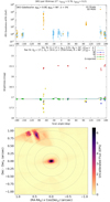 |
Fig. B.9. SourceID 379163256239241216: Scan-angle signatures and image reconstructed by SEAPipe. |
-- ADQL query on DR3, aiming at sources with many transits
-- and "intermediate" magnitudes: (leading to ~132k,
-- after which a XM can be done)
SELECT source_id,ra,ra_error,dec,dec_error,parallax,
parallax_error,pmra,pmra_error,pmdec,pmdec_error,
astrometric_params_solved,matched_transits,
ipd_gof_harmonic_amplitude,ipd_gof_harmonic_phase,
ipd_frac_multi_peak,ipd_frac_odd_win,
phot_g_n_obs,phot_g_mean_mag,phot_variable_flag
FROM gaiadr3.gaia_source
WHERE (in_andromeda_survey = 'true')
AND (matched_transits > 50)
AND (phot_g_mean_mag BETWEEN 12.0 AND 19.0),
Finally, Fig. B.10 shows another example obtained with the same query. In this case, we have three sources, with separations of 560 and 1040 mas from the source shown in the figure. As otherwise expected, the effects on both G and BP/RP are significant. Despite the rejected G measurements, the pair model appears to determine sensible values.
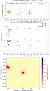 |
Fig. B.10. SourceID 388877407113709056: Scan-angle signatures and image reconstructed by SEAPipe. |
B.3. Wing of a bright star in DR3
With the query
-- ADQL query on DR3, aiming at bright stars,
-- then XM'ed with previous query:
SELECT source_id,ra,ra_error,dec,dec_error,parallax,
parallax_error,pmra,pmra_error,pmdec,pmdec_error,
astrometric_params_solved,matched_transits,
ipd_gof_harmonic_amplitude,ipd_gof_harmonic_phase,
ipd_frac_multi_peak,ipd_frac_odd_win,phot_g_n_obs,
phot_g_mean_mag,phot_variable_flag
FROM gaiadr3.gaia_source
WHERE (in_andromeda_survey = 'true')
AND (matched_transits > 50)
AND (phot_g_mean_mag < 8.0)
plus a simplistic cross match, we also obtained an example of a DR3 source that lies close to a bright source (magnitude 7.3). With this, we wished to verify whether the PSF wings of the nearby bright source can also cause scan-angle artefacts. Fig. B.11 indeed shows a remarkable peak in the flux at a specific angle, with a smaller peak at 180 degrees of it. They were both rejected by variability processing. BP and RP photometry could not be determined here, most probably due to the contamination of the bright neighbour. Interestingly, in this case, the rexf, G and ripd, G correlations are both nearly zero, as is the IPD GoF harmonics. Only the fraction of transits with multiple peaks provides an indication: Transits with multiple peaks are indeed at about the same angles at which we see the strong variations in G photometry.
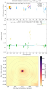 |
Fig. B.11. Example of a source affected by the PSF wing of a nearby bright source. SourceID 385771836519005184: Scan-angle signatures and image reconstructed by SEAPipe. |
B.4. Blind search for resolved or unresolved close pairs in DR3
With an adequate query on DR3 GaiaSource, making use of the several multiplicity indicators (ipd_frac_multi_peak, ipd_gof_harmonic_amplitude),
-- ADQL query on DR3, aiming at good candidates
-- to be an unresolved pair:
SELECT source_id,ra,ra_error,dec,dec_error,
matched_transits,ipd_gof_harmonic_amplitude,
ipd_gof_harmonic_phase,ipd_frac_multi_peak,
ipd_frac_odd_win,phot_g_n_obs,phot_g_mean_mag,
phot_variable_flag FROM gaiadr3.gaia_source
WHERE (in_andromeda_survey = 'true')
AND (ipd_frac_multi_peak BETWEEN 30 AND 50)
AND (ipd_gof_harmonic_amplitude >= 0.4)
AND (astrometric_params_solved = 3)
AND (phot_g_mean_mag BETWEEN 12 AND 19.0)
AND (matched_transits >= 50)
AND (ipd_frac_odd_win < 20)
we can obtain good candidates of either resolved or unresolved close pairs. From the resulting list of sources, we can obtain the public epoch photometry, which can lead to figures such as Fig. B.12, Fig. B.13, or Fig. B.14. The second source is specially interesting because the Variability flag was set for this source. All sources show the usual effects: the brighter, scan-angle-dependent G fluxes correspond to transits without a detected secondary peak. Thus, overall, it seems to demonstrate that the IDU IPD masking of secondary peaks behaved as expected. Regarding the IPD GoF harmonics, the third case shown here has one of the highest values, but in general, the Spearman rexf, G correlation seems to be a more reliable and useful indicator of contaminants. The fit to the pair model achieved in Fig. B.14 is excellent.
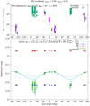 |
Fig. B.12. SourceID 367388551858425344: Scan-angle signatures. |
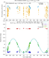 |
Fig. B.13. SourceID 383556286230747520: Scan-angle signatures. |
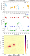 |
Fig. B.14. SourceID 380538569192874112: Scan-angle signatures and image reconstructed by SEAPipe. |
B.5. Galaxies in DR3
Finally, with the query
-- ADQL query on DR3, aiming at Galaxies with morph params:
SELECT source_id,ra,ra_error,dec,dec_error,
parallax,parallax_error,pmra,pmra_error,
pmdec,pmdec_error,astrometric_params_solved,
matched_transits,ipd_gof_harmonic_amplitude,
ipd_gof_harmonic_phase,ipd_frac_multi_peak,
ipd_frac_odd_win,phot_g_n_obs,phot_g_mean_mag,
phot_variable_flag FROM gaiadr3.gaia_source
WHERE (in_andromeda_survey = 'true')
AND (matched_transits >= 30)
AND (phot_g_mean_mag < = 20.0)
AND (in_galaxy_candidates = 'true')
AND (astrometric_params_solved = 3)
AND (source_id IN (select source_id from
gaiadr3.galaxy_candidates where
gaiadr3.galaxy_candidates.radius_de_vaucouleurs
       IS NOT NULL)),
we also tested the case of galaxies for which we even have morphological values, such as the radius. The example shown in Fig. 9 shows significant variations in all bands, but possibly a clearer scan-angle signature in G (as otherwise expected). When the internal DR3 IPD epoch GoF values are inspected, the signature is clearer. This is revealed by the higher value in the ripd, G Spearman correlation than in rexf, G. For completeness, Fig. B.15 shows another example for a high-ellipticity galaxy, and Fig. B.16 shows an example for a low-ellipticity galaxy.
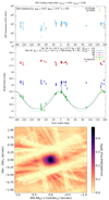 |
Fig. B.15. SourceID 364175332206026368: Scan-angle signatures and image reconstructed by SEAPipe. |
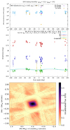 |
Fig. B.16. SourceID 373852271480563968: Scan-angle signatures and image reconstructed by SEAPipe. |
B.6. DR3 spectroscopic binaries
Gaia DR3 contains some SB1 sources whose periods are very close to the precession period of the satellite (63 days), and thus they might be spurious. In Fig. B.17 and B.18 we show two examples, which were furthermore identified as variable stars.
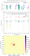 |
Fig. B.17. SourceID 415146526611154176: Scan-angle signatures and image reconstructed by SEAPipe. |
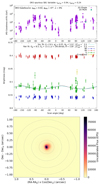 |
Fig. B.18. SourceID 5815369024263284352: Scan-angle signatures and image reconstructed by SEAPipe. |
Appendix C: Sky distribution of observed and simulated spurious period peaks
In this section, we show the sky distribution of the most prominent photometric and astrometric spurious period peaks identified in Figs. 22, 23, and 24 of Sect. 5.4. It is important to realise that the photometric and astrometric unpublished data are sampled non-uniformly over the sky, as shown in Fig. C.1. The Galactic source density is very strongly imprinted on the sky sampling, meaning that this pattern will thus naturally be present in any of the observed period subsets shown in the left panels of Figs. C.2, C.3, C.6, and C.7.
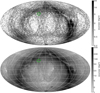 |
Fig. C.1. Ecliptic Aitoff projection with longitude zero at the centre and increasing to the left. Top: Sky density of the (unpublished) all-sky photometric sample, subsets of which for different period ranges are shown in Figs. C.2 and C.3. Bottom: Sky density of the (unpublished) all-sky astrometric sample, subsets of which for different period ranges are shown in Figs. C.6 and C.7. Both samples are introduced in Sect. 4.1. The green circle indicates the location of the GAPS catalogue (see Fig. 23). |
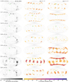 |
Fig. C.2. Ecliptic Aitoff projection of the photometric data presented in Fig. 22. Left: Source density of the photometric peaks for the all-sky sample (top panel of Fig. 22). Right: Result of the all-sky uniform simulations of our noiseless sampled bias model (panels 2 and 3 of Fig. 22). They are colour-coded with the percentage of phases (position angles) that results in this peak: A low value means that only specific phasing of the scan-angle signal will result in a particular peak being observed at the given location. The green circle indicates the location of the GAPS catalogue (see Fig. 23). In all sky plots, longitude zero is at the centre and increasing to the left. |
 |
Fig. C.4. Example public folded G-band light curves for different period peaks, derived by the multi-harmonic modelling following a generalised least-squares period search as described in Sect. 4.1. The source id is provided in the top right corner. Additional information is available in Table 1 for sources with an asterisk. In general, the sources either have very high ripd, G, rexf, G, or aG significance (but always a low false-alarm probability). |
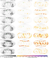 |
Fig. C.6. Ecliptic Aitoff projection of the astrometric period data presented in Fig. 24. Left: Source density of the astrometric peaks for the all-sky sample (top panel of Fig. 24). Right: Result of the all-sky uniform simulations of our noiseless sampled bias model (panels 2 and 3 of Fig. 24). They are colour-coded with the percentage of phases (position angles) that results in this peak: a low value means that only specific phasing of the scan-angle signal will result in a particular peak being observed at the given location. The green circle indicates the location of the GAPS catalogue. In all sky plots longitude zero is at the centre and increases to the left. |
In addition to the sky maps, we also include example folded time-series of public photometry for the main spurious peaks in Figs. C.4 and C.5.
Appendix D: Scan position angle in ecliptic coordinates
For use in Sect. 2.1, we here derive an expression for the position angle of a scan relative to local ecliptic north, ψecl (here generically labelled θecl), given the position of the source, (α, δ), and the position angle of the scan relative to local equatorial north, ψequ (here generically labelled θequ). Although we speak about the scan position angle, the results apply to any position angle. We therefore use the more generic position-angle symbol θ.
The geometry of the scan is shown in Fig. D.1. The difference between the two position angles, ϕ = θecl − θequ, is the angle at the source (S) in the spherical triangle it forms with the north celestial pole (NCP) and the north ecliptic pole (NEP), NCP–S–NEP, in which the other sides and angles depend on the equatorial and ecliptic coordinates of the source, (α, δ) and (λ, β), and the obliquity of the ecliptic, ϵ = 84381.41100 arcsec. From the sine theorem, we have
 (D.1)
(D.1)
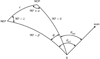 |
Fig. D.1. Geometry of the scan across a source at S relative to the north celestial pole and north ecliptic pole, as viewed from outside the celestial sphere. |
and from the cosine theorem,
 (D.2)
(D.2)
or
 (D.3)
(D.3)
From the last two equations, it is possible to solve ϕ without quadrant ambiguity, but the equations involve not only (α, δ), but also β, which may be inconvenient. However, from the cosine theorem, we also have
 (D.4)
(D.4)
which after insertion in Eq. (D.3) and division by cos δ gives
 (D.5)
(D.5)
Combination of Eqs. (D.1) and (D.5) now gives
 (D.6)
(D.6)
from which
 (D.7)
(D.7)
gives the ecliptic position angle in the interval [0, 2π). This calculation is implemented in the MATLAB function scanPaEcl reproduced below. As a test example, α = 1.1, δ = −0.5, and θequ = 1.7 gives ϕ = 0.276758777373696 and θecl = 1.9767587773737.
function [thetaEcl,phi] = scanPaEcl(alpha,delta,thetaEqu)
% Given the position of a source (alpha,delta) [rad] and the
% position angle of the scan at the source in the local
% equatorial system, thetaEqu [rad],  this function returns
% the position angle of the scan in the local ecliptic
% system, thetaEcl [rad] and (optionally) the difference phi.
%
% Lennart Lindegren 2022-05-16

% obliquity of the ecliptic [rad]:
epsilon = 84381.41100 * pi/(180*3600);

ce = cos(epsilon);
se = sin(epsilon);
ca = cos(alpha);
sa = sin(alpha);
cd = cos(delta);
sd = sin(delta);
phi = atan2(se*ca, ce*cd+se*sd*sa);
thetaEcl = mod(thetaEqu + phi, 2*pi);

end
Figure D.1 was drawn for the case when ϕ > 0, but (D.6)–(D.7) are completely general and valid across the entire sky, except at the ecliptic pole (cos β = 0), where θecl is undefined. Figure D.2 shows the distribution of ϕ for random positions.
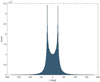 |
Fig. D.2. Histogram of ϕ for 106 random points of the sphere. |
Appendix E: Gaia acknowledgements
This work presents results from the European Space Agency (ESA) space mission Gaia. Gaia data are being processed by the Gaia Data Processing and Analysis Consortium (DPAC). Funding for the DPAC is provided by national institutions, in particular the institutions participating in the Gaia MultiLateral Agreement (MLA). The Gaia mission website is https://www.cosmos.esa.int/gaia. The Gaia archive website is https://archives.esac.esa.int/gaia.
The Gaia mission and data processing have financially been supported by, in alphabetical order by country:
-
the Algerian Centre de Recherche en Astronomie, Astrophysique et Géophysique of Bouzareah Observatory;
-
the Austrian Fonds zur Förderung der wissenschaftlichen Forschung (FWF) Hertha Firnberg Programme through grants T359, P20046, and P23737;
-
the BELgian federal Science Policy Office (BELSPO) through various PROgramme de Développement d’Expériences scientifiques (PRODEX) grants and the Polish Academy of Sciences – Fonds Wetenschappelijk Onderzoek through grant VS.091.16N, and the Fonds de la Recherche Scientifique (FNRS), and the Research Council of Katholieke Universiteit (KU) Leuven through grant C16/18/005 (Pushing AsteRoseismology to the next level with TESS, GaiA, and the Sloan DIgital Sky SurvEy – PARADISE);
-
the Brazil-France exchange programmes Fundação de Amparo à Pesquisa do Estado de São Paulo (FAPESP) and Coordenação de Aperfeicoamento de Pessoal de Nível Superior (CAPES) – Comité Français d’Evaluation de la Coopération Universitaire et Scientifique avec le Brésil (COFECUB);
-
the Chilean Agencia Nacional de Investigación y Desarrollo (ANID) through Fondo Nacional de Desarrollo Científico y Tecnológico (FONDECYT) Regular Project 1210992 (L. Chemin);
-
the National Natural Science Foundation of China (NSFC) through grants 11573054, 11703065, and 12173069, the China Scholarship Council through grant 201806040200, and the Natural Science Foundation of Shanghai through grant 21ZR1474100;
-
the Tenure Track Pilot Programme of the Croatian Science Foundation and the École Polytechnique Fédérale de Lausanne and the project TTP-2018-07-1171 ‘Mining the Variable Sky’, with the funds of the Croatian-Swiss Research Programme;
-
the Czech-Republic Ministry of Education, Youth, and Sports through grant LG 15010 and INTER-EXCELLENCE grant LTAUSA18093, and the Czech Space Office through ESA PECS contract 98058;
-
the Danish Ministry of Science;
-
the Estonian Ministry of Education and Research through grant IUT40-1;
-
the European Commission’s Sixth Framework Programme through the European Leadership in Space Astrometry (ELSA) Marie Curie Research Training Network (MRTN-CT-2006-033481), through Marie Curie project PIOF-GA-2009-255267 (Space AsteroSeismology & RR Lyrae stars, SAS-RRL), and through a Marie Curie Transfer-of-Knowledge (ToK) fellowship (MTKD-CT-2004-014188); the European Commission’s Seventh Framework Programme through grant FP7-606740 (FP7-SPACE-2013-1) for the Gaia European Network for Improved data User Services (GENIUS) and through grant 264895 for the Gaia Research for European Astronomy Training (GREAT-ITN) network;
-
the European Cooperation in Science and Technology (COST) through COST Action CA18104 ‘Revealing the Milky Way with Gaia (MW-Gaia)’;
-
the European Research Council (ERC) through grants 320360, 647208, and 834148 and through the European Union’s Horizon 2020 research and innovation and excellent science programmes through Marie Skłodowska-Curie grant 745617 (Our Galaxy at full HD – Gal-HD) and 895174 (The build-up and fate of self-gravitating systems in the Universe) and grants 687378 (Small Bodies: Near and Far), 682115 (Using the Magellanic Clouds to Understand the Interaction of Galaxies), 695099 (A sub-percent distance scale from binaries and Cepheids – CepBin), 716155 (Structured ACCREtion Disks – SACCRED), 951549 (Sub-percent calibration of the extragalactic distance scale in the era of big surveys – UniverScale), and 101004214 (Innovative Scientific Data Exploration and Exploitation Applications for Space Sciences – EXPLORE);
-
the European Science Foundation (ESF), in the framework of the Gaia Research for European Astronomy Training Research Network Programme (GREAT-ESF);
-
the European Space Agency (ESA) in the framework of the Gaia project, through the Plan for European Cooperating States (PECS) programme through contracts C98090 and 4000106398/12/NL/KML for Hungary, through contract 4000115263/15/NL/IB for Germany, and through PROgramme de Développement d’Expériences scientifiques (PRODEX) grant 4000127986 for Slovenia;
-
the Academy of Finland through grants 299543, 307157, 325805, 328654, 336546, and 345115 and the Magnus Ehrnrooth Foundation;
-
the French Centre National d’Études Spatiales (CNES), the Agence Nationale de la Recherche (ANR) through grant ANR-10-IDEX-0001-02 for the ‘Investissements d’avenir’ programme, through grant ANR-15-CE31-0007 for project ‘Modelling the Milky Way in the Gaia era’ (MOD4Gaia), through grant ANR-14-CE33-0014-01 for project ‘The Milky Way disc formation in the Gaia era’ (ARCHEOGAL), through grant ANR-15-CE31-0012-01 for project ‘Unlocking the potential of Cepheids as primary distance calibrators’ (UnlockCepheids), through grant ANR-19-CE31-0017 for project ‘Secular evolution of galaxies’ (SEGAL), and through grant ANR-18-CE31-0006 for project ‘Galactic Dark Matter’ (GaDaMa), the Centre National de la Recherche Scientifique (CNRS) and its SNO Gaia of the Institut des Sciences de l’Univers (INSU), its Programmes Nationaux: Cosmologie et Galaxies (PNCG), Gravitation Références Astronomie Métrologie (PNGRAM), Planétologie (PNP), Physique et Chimie du Milieu Interstellaire (PCMI), and Physique Stellaire (PNPS), the ‘Action Fédératrice Gaia’ of the Observatoire de Paris, the Région de Franche-Comté, the Institut National Polytechnique (INP) and the Institut National de Physique nucléaire et de Physique des Particules (IN2P3) co-funded by CNES;
-
the German Aerospace Agency (Deutsches Zentrum für Luft- und Raumfahrt e.V., DLR) through grants 50QG0501, 50QG0601, 50QG0602, 50QG0701, 50QG0901, 50QG1001, 50QG1101, 50QG1401, 50QG1402, 50QG1403, 50QG1404, 50QG1904, 50QG2101, 50QG2102, and 50QG2202, and the Centre for Information Services and High Performance Computing (ZIH) at the Technische Universität Dresden for generous allocations of computer time;
-
the Hungarian Academy of Sciences through the Lendület Programme grants LP2014-17 and LP2018-7 and the Hungarian National Research, Development, and Innovation Office (NKFIH) through grant KKP-137523 (‘SeismoLab’);
-
the Science Foundation Ireland (SFI) through a Royal Society – SFI University Research Fellowship (M. Fraser);
-
the Israel Ministry of Science and Technology through grant 3-18143 and the Tel Aviv University Center for Artificial Intelligence and Data Science (TAD) through a grant;
-
the Agenzia Spaziale Italiana (ASI) through contracts I/037/08/0, I/058/10/0, 2014-025-R.0, 2014-025-R.1.2015, and 2018-24-HH.0 to the Italian Istituto Nazionale di Astrofisica (INAF), contract 2014-049-R.0/1/2 to INAF for the Space Science Data Centre (SSDC, formerly known as the ASI Science Data Center, ASDC), contracts I/008/10/0, 2013/030/I.0, 2013-030-I.0.1-2015, and 2016-17-I.0 to the Aerospace Logistics Technology Engineering Company (ALTEC S.p.A.), INAF, and the Italian Ministry of Education, University, and Research (Ministero dell’Istruzione, dell’Università e della Ricerca) through the Premiale project ‘MIning The Cosmos Big Data and Innovative Italian Technology for Frontier Astrophysics and Cosmology’ (MITiC);
-
the Netherlands Organisation for Scientific Research (NWO) through grant NWO-M-614.061.414, through a VICI grant (A. Helmi), and through a Spinoza prize (A. Helmi), and the Netherlands Research School for Astronomy (NOVA);
-
the Polish National Science Centre through HARMONIA grant 2018/30/M/ST9/00311 and DAINA grant 2017/27/L/ST9/03221 and the Ministry of Science and Higher Education (MNiSW) through grant DIR/WK/2018/12;
-
the Portuguese Fundação para a Ciência e a Tecnologia (FCT) through national funds, grants SFRH/BD/128840/2017 and PTDC/FIS-AST/30389/2017, and work contract DL 57/2016/CP1364/CT0006, the Fundo Europeu de Desenvolvimento Regional (FEDER) through grant POCI-01-0145-FEDER-030389 and its Programa Operacional Competitividade e Internacionalização (COMPETE2020) through grants UIDB/04434/2020 and UIDP/04434/2020, and the Strategic Programme UIDB/00099/2020 for the Centro de Astrofísica e Gravitação (CENTRA);
-
the Slovenian Research Agency through grant P1-0188;
-
the Spanish Ministry of Economy (MINECO/FEDER, UE), the Spanish Ministry of Science and Innovation (MICIN), the Spanish Ministry of Education, Culture, and Sports, and the Spanish Government through grants BES-2016-078499, BES-2017-083126, BES-C-2017-0085, ESP2016-80079-C2-1-R, ESP2016-80079-C2-2-R, FPU16/03827, PDC2021-121059-C22, RTI2018-095076-B-C22, and TIN2015-65316-P (‘Computación de Altas Prestaciones VII’), the Juan de la Cierva Incorporación Programme (FJCI-2015-2671 and IJC2019-04862-I for F. Anders), the Severo Ochoa Centre of Excellence Programme (SEV2015-0493), and MICIN/AEI/10.13039/501100011033 (and the European Union through European Regional Development Fund ‘A way of making Europe’) through grant RTI2018-095076-B-C21, the Institute of Cosmos Sciences University of Barcelona (ICCUB, Unidad de Excelencia ‘María de Maeztu’) through grant CEX2019-000918-M, the University of Barcelona’s official doctoral programme for the development of an R+D+i project through an Ajuts de Personal Investigador en Formació (APIF) grant, the Spanish Virtual Observatory through project AyA2017-84089, the Galician Regional Government, Xunta de Galicia, through grants ED431B-2021/36, ED481A-2019/155, and ED481A-2021/296, the Centro de Investigación en Tecnologías de la Información y las Comunicaciones (CITIC), funded by the Xunta de Galicia and the European Union (European Regional Development Fund – Galicia 2014-2020 Programme), through grant ED431G-2019/01, the Red Española de Supercomputación (RES) computer resources at MareNostrum, the Barcelona Supercomputing Centre – Centro Nacional de Supercomputación (BSC-CNS) through activities AECT-2017-2-0002, AECT-2017-3-0006, AECT-2018-1-0017, AECT-2018-2-0013, AECT-2018-3-0011, AECT-2019-1-0010, AECT-2019-2-0014, AECT-2019-3-0003, AECT-2020-1-0004, and DATA-2020-1-0010, the Departament d’Innovació, Universitats i Empresa de la Generalitat de Catalunya through grant 2014-SGR-1051 for project ‘Models de Programació i Entorns d’Execució Parallels’ (MPEXPAR), and Ramon y Cajal Fellowship RYC2018-025968-I funded by MICIN/AEI/10.13039/501100011033 and the European Science Foundation (‘Investing in your future’);
-
the Swedish National Space Agency (SNSA/Rymdstyrelsen);
-
the Swiss State Secretariat for Education, Research, and Innovation through the Swiss Activités Nationales Complémentaires and the Swiss National Science Foundation through an Eccellenza Professorial Fellowship (award PCEFP2_194638 for R. Anderson);
-
the United Kingdom Particle Physics and Astronomy Research Council (PPARC), the United Kingdom Science and Technology Facilities Council (STFC), and the United Kingdom Space Agency (UKSA) through the following grants to the University of Bristol, the University of Cambridge, the University of Edinburgh, the University of Leicester, the Mullard Space Sciences Laboratory of University College London, and the United Kingdom Rutherford Appleton Laboratory (RAL): PP/D006511/1, PP/D006546/1, PP/D006570/1, ST/I000852/1, ST/J005045/1, ST/K00056X/1, ST/K000209/1, ST/K000756/1, ST/L006561/1, ST/N000595/1, ST/N000641/1, ST/N000978/1, ST/N001117/1, ST/S000089/1, ST/S000976/1, ST/S000984/1, ST/S001123/1, ST/S001948/1, ST/S001980/1, ST/S002103/1, ST/V000969/1, ST/W002469/1, ST/W002493/1, ST/W002671/1, ST/W002809/1, and EP/V520342/1.
The GBOT programme uses observations collected at (i) the European Organisation for Astronomical Research in the Southern Hemisphere (ESO) with the VLT Survey Telescope (VST), under ESO programmes 092.B-0165, 093.B-0236, 094.B-0181, 095.B-0046, 096.B-0162, 097.B-0304, 098.B-0030, 099.B-0034, 0100.B-0131, 0101.B-0156, 0102.B-0174, and 0103.B-0165; and (ii) the Liverpool Telescope, which is operated on the island of La Palma by Liverpool John Moores University in the Spanish Observatorio del Roque de los Muchachos of the Instituto de Astrofísica de Canarias with financial support from the United Kingdom Science and Technology Facilities Council, and (iii) telescopes of the Las Cumbres Observatory Global Telescope Network.
All Tables
Overview of source examples in this work that have scan-angle-dependent signals, along with diagnostic statistics and fitted parameters.
gaia_dr3.vari_spurious_signalsGaia archive table fields. See the Gaia archive documentation for more detailed descriptions.
All Figures
|
Fig. 1. Overview of the Gaia scanning law. Left: during the nominal scanning law, the spin axis z makes overlapping loops around the Sun at a separation of 45° and rate of 5.8 cycles yr−1. Right: one source at point a may be scanned whenever z is 90° from a, that is, on the great circle A at z1, z2, z3, etc. Reproduction with permission of Fig. 7 in Gaia Collaboration (2016). |
| In the text | |
|
Fig. 2. Ecliptic coordinate plots with longitude zero at the centre and increasing to the left. Top panel: simulated number of field-of-view observations during the nominal scanning law phase of the Gaia DR3 time range. Bottom panel: sky density of the published Gaia DR3 sources. |
| In the text | |
|
Fig. 3. Ecliptic scan-angle distribution for the nominal scanning law during the Gaia DR3 time range. For a certain ecliptic latitude (horizontal slice), the colour represents the occupancy percentage per 1° scan-angle bin (summing up to 100% over all scan angles) to highlight non-uniformities in the scan-angle distribution at different ecliptic latitudes. Top panel: distribution for sources along a half-circle slice at ecliptic longitude λ = 90°. Bottom panel: same as top panel, but for an all-sky uniform HEALPix grid of sources (that is, all ecliptic longitudes for a given latitude). The strong imbalance of scan angles for sources |β|≤45° has a strong impact on the propagation strength of certain scan-angle-dependent signals; see text for details. |
| In the text | |
|
Fig. 4. Time series of the ecliptic scan-angle distribution during the Gaia DR3 NSL time range for five ecliptic latitudes along the half-circle slice with ecliptic longitude λ = 90° (same as the top panel of Fig. 3). Each point is semi-transparent, so that a darker colour means more observations. Blue cyclic lines illustrate the slopes due to the yearly rotation around the Sun. The histogram on the right side has a bin size of 32.7° (360/11) and shows the relative distribution of scan angles, corresponding to the top panel of Fig. 3 for the specified ecliptic latitudes. |
| In the text | |
|
Fig. 5. Sky distribution in ecliptic coordinates of extragalactic sources analysed in terms of surface brightness profile in Gaia DR3, colour-coded with the angular coverage of the sources. The non-linear shader table reveals the NSL pattern. |
| In the text | |
|
Fig. 6. Sky-projected illustration of the rough zones in which equal-brightness optical binary stars (two red crosses) at angular separation ρ and position angle θ can be resolved by Gaia. In the partially resolved region, the stars are resolved into two components depending on the scan angle ψi of the observation i, because of the asymmetric PSF, which has the highest spatial resolution in the along-scan direction. The bottom right inset shows a typical PSF profile (Fabricius et al. 2016) that is rotated and scaled in the background image to represent the expected PSF of the upper right component of the binary star for the given scan angle. East direction (increasing RA) is towards the left. |
| In the text | |
|
Fig. 7. SourceID 389636619892245248: Scan-angle signatures from a partially resolved double star with similar magnitudes and a separation of about 130 mas between the two components (determined by IDU for DR4). The top panel shows the unpublished IPD epoch GoF values determined by IDU in DR3, where we indicate the scans for which the IPD detected multiple peaks. The central panel shows the brightness in the G band and in the BP and RP photometry as provided by the epoch-photometry table published in DR3, to illustrate the differences in that instrument. It also includes the fits to G using Eq. (4) (pair model) and Eq. (5) (sinusoidal model). The bottom panel shows the image reconstructed by SEAPipe, with dashed grey circles at increasing radii in steps of 250 mas from the image centre. See text for further details. |
| In the text | |
|
Fig. 8. SourceID 382074694311961856: Scan-angle signatures (top and central panels) and image reconstructed by SEAPipe (bottom panel) from a resolved double star with a separation of about 360 mas between the two components, available as two separate sources in DR3 (only one of the two sources is shown in the top and central panels). See text and Fig. 7 for further details. |
| In the text | |
|
Fig. 9. Galaxy LEDA 2112767 (Paturel et al. 2003), sourceID 366951667785042688: Scan-angle signatures (top and central panels) and image reconstructed by SEAPipe (bottom panel). This galaxy was published in Gaia DR3 with a moderate ellipticity. See text and Fig. 7 for further details. |
| In the text | |
|
Fig. 10. Comparison of the position angle of extended galaxies measured with Gaia data with the ipd_gof_harmonic_phase parameter. |
| In the text | |
|
Fig. 11. Example of two sources causing blended spectra in some of the observations. The rectangular shapes show the footprint of the observing window for real transits over one of the two sources. In the transits highlighted in green, the secondary source is located beyond the window, while both sources are inside the window for grey transits. The dispersion direction is along the major side of the observing window. |
| In the text | |
|
Fig. 12. Examples of crowding effects on the photometry for six sources, each with a different colour. From top to bottom, we show the epoch-corrected flux excess C* as a function of epoch G, GBP, and GRP. Sources shown as crosses were estimated as crowded in every BP/RP transit. Sources shown as diamonds were estimated as crowded in only a few transits. |
| In the text | |
|
Fig. 13. Example demonstrating how insufficient astrometric modelling leads to incorrect RV determinations. Top panel: motion of Gaia DR3 6631710606341412096 on the sky with respect to its reference position in the reference system moving with Gaia, as predicted from the five-parameter single-star AGIS solution (solid blue line), compared with the position predicted by the NSS AstroSpectroSB1 solution (dot-dashed red line), which included the Keplerian orbit. Circles show the positions at which the epoch RV were measured, and the arrows show the scanning direction at the epoch. Bottom panel: RV data, folded in phase, as provided by the DR3 pipeline (blue dots) and the data corrected for the displacement (in red), compared with the radial velocity predicted by the AstroSpectroSB1 solution (green line). |
| In the text | |
|
Fig. 14. Top panel: image of the source Gaia DR3 5648209549925093504 produced by SEAPipe. Middle panel: RV data of Gaia DR3 5648209549925093504, folded in phase, as provided by the DR3 pipeline (black dots), compared with the SB1 solution provided in DR3 (blue line). Bottom panel: RV data as a function of the scan angle ψ, compared with a sinusoidal signal as predicted by Eq. (2). |
| In the text | |
|
Fig. 15. Spectrum of Gaia DR3 2006840790676091776, contaminated by the nearby source Gaia DR3 2006840790679122688 recorded in a transit. The solid vertical red lines show the real position of the Ca II triplet lines of Gaia DR3 2006840790676091776, and the dot-dashed green lines show the position of the same lines as found by the pipeline. |
| In the text | |
|
Fig. 16. Period distributions of (largely unpublished) Gaia data to show the diversity and (dis)similarities of various peak locations and amplitudes. See also Figs. 22–24 for comparison with period search results on simulated scan-angle signals that qualitatively reproduce these peaks. |
| In the text | |
|
Fig. 17. Distribution of false-alarm probabilities of the two photometric samples shown in Fig. 16, illustrating the highly significant nature of most of the spurious periods. |
| In the text | |
|
Fig. 18. Simulation of the magnitude bias, ΔG, for the brighter component of a close source pair for five different separations and as a function of the difference between the position angle of the scan and the position angle of the fainter component. The magnitude differences in the top panel are 0.5 mag and in the bottom panel 2.5 mag. |
| In the text | |
|
Fig. 19. Simulation of the positional bias for the brighter component of a close source pair for five different separations and as a function of the difference between the position angle of the scan and the position angle of the fainter component. The magnitude differences in the top panel are 0.5 mag and in the bottom panel 2.5 mag. |
| In the text | |
|
Fig. 20. Astrometric along-scan bias δη of Eq. (6) as a function of scan angle ψ for a flux ratio f = 0.656 (ΔG = 0.46, mass ratio q = 0.9), and position angle θ = 0°. Left to right: source separation ρ = 100, 200, 300, and 400 mas. Top panels: total bias δη (blue line), and a cosine fit (dashed red line) that will propagate into a position bias. Bottom panels: residuals of the cosine fit (magenta line) that can bias other source parameters. |
| In the text | |
|
Fig. 21. Same as Fig. 20, but for a flux ratio f = 2.8 × 10⁻³ (ΔG = 6.38), corresponding to the mass ratio q = 0.23 of a typical binary. |
| In the text | |
|
Fig. 22. Comparison between the unpublished observed period distribution of an all-sky photometric sample (top panel, red line, same as top panel of Fig. 16) and that predicted by our noiseless sampled bias model of Eq. (7) for different scan-angle harmonics k (purple lines in following panels). See Figs. C.2 and C.3 for ecliptic sky maps and Figs. C.4 and C.5 for spurious-period-folded time series of the most prominent peaks. |
| In the text | |
|
Fig. 23. Same as Fig. 22, but for the published GAPS photometry. The top panel (orange line) shows the same data as in the second panel of Fig. 16. The green circles in Figs. C.2 and C.3 show ecliptic sky maps of the most prominent peaks. |
| In the text | |
|
Fig. 24. Comparison between the unpublished period distribution of an all-sky astrometric orbit sample (top panel, blue line, same as the bottom panel of Fig. 16) and that predicted by our fits to the noiseless sampled bias model of Eq. (7) for different scan-angle harmonics k (purple lines in the following panels). See Figs. C.6 and C.7 for ecliptic sky maps of the most prominent peaks. |
| In the text | |
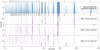 |
Fig. 25. Same unpublished data as Fig. 24, now showing the period-eccentricity relation. |
| In the text | |
|
Fig. 26. Same unpublished data as Fig. 24, now showing the period vs fitted semi-major axis, illustrating that the observed semi-major axes typically lie between 0.1 and 10 mas (top panel), and showing that the orbital solutions fitted to the noiseless sampled bias model with amplitude 1 mas induce semi-major axes of one to several milliarcseconds (following panels). |
| In the text | |
|
Fig. 27. Same unpublished data as Fig. 24, now showing the period vs fitted semi-major axis significance, illustrating the highly significant nature of most of the observed orbits (top panel), and even more so for the orbital solutions fitted to the noiseless sampled bias model with amplitude 1 mas (following panels). |
| In the text | |
|
Fig. 28. Distribution of sources published in GAPS. The top panel shows the same data as in the second panel of Fig. 16. The following panels illustrate the distributions of various statistics that can be used to diagnose possible scan-angle-dependent signals; see text for details. An example filter has been created to show the effect on the period distribution. The total source counts are only for the period range of 10−500 d. |
| In the text | |
|
Fig. 29. Parameter domain map for the filters based on the main source statistics. |
| In the text | |
|
Fig. A.1. Correlations based on the published photometric time series in Gaia DR3. Top panels: Histograms of the number of available observations for the different correlation coefficients. Second to fourth panel rows: ipd correlation coefficients (Sect. 6.1). Fifth to seventh panel rows: Corrected excess factor correlation coefficients (Sect. 6.2). On the right side, a histogram illustrates the distribution of each correlation coefficient. The left panels contain the values for the 10.5 million variables, and the right panels show the values for the 1.3 million sources in GAPS. The heat maps are value normalised per number of observation bin to highlight the level of parameter spread. The histograms on the right sides represent the true count distribution for each parameter. |
| In the text | |
|
Fig. A.2. Density plots of the rexf, G vs ripd, G correlation with at least 20 observations for each statistic (N3band ≥ 20 and NnoEpsl, G ≥ 20). See Sect. 6 for a discussion. |
| In the text | |
|
Fig. A.3. Density plot of the relation between ripd, G and |
| In the text | |
|
Fig. A.4. Density plots of various parameters in relation to the significance of aG, the amplitude of the small-separation binary model fit to the G-band photometry (Eq. 5). The white vertical line indicates a significance threshold of 6, above which the fitted amplitude is more likely due to a scan-angle-dependent signal. In the top panels, the same low |
| In the text | |
|
Fig. A.5. Density of the median G-band magnitude dependence of aG, the amplitude of the small-separation binary model fit to the G-band photometry (Eq. 5). The top left inset images shows the same data colour-coded with the median ripd, G and rexf, G, respectively, both ranging between 0 (blue) and 1 (red). See Sect. 6.3 for discussion. Plots are restricted to sources with N3band ≥ 20 and NnoEpsl, G ≥ 20. |
| In the text | |
|
Fig. A.6. Density plot of the relation between ipd_gof_harmonic_amplitude and aG (the amplitude of the fit to the G-band photometry (Eq. 5). For ipd_gof_harmonic_amplitude ≳0.07, this relation is very strong (see Sects. 3.1.3, 6.3, and 7.3 for a more detailed discussion). Plots for N3band ≥ 20 and NnoEpsl, G ≥ 20. |
| In the text | |
|
Fig. B.1. SourceID 388466602081536640: Scan-angle signatures. |
| In the text | |
|
Fig. B.2. SourceID 378810450446502400: Scan-angle signatures and image reconstructed by SEAPipe. |
| In the text | |
|
Fig. B.3. SourceID 385804856230839552: Scan-angle signatures (top panels) and raw windows for some of its transits (bottom panels). |
| In the text | |
|
Fig. B.4. SourceID 382159975182923264: Scan-angle signatures, image reconstructed by SEAPipe, and two of the CCD observations taken at different scan angles. |
| In the text | |
|
Fig. B.5. SourceID 376045247423005184: Scan-angle signatures. |
| In the text | |
|
Fig. B.6. SourceID 385844060692409344: Scan-angle signatures. |
| In the text | |
|
Fig. B.7. SourceID 385367010081173504: Scan-angle signatures and image reconstructed by SEAPipe. |
| In the text | |
|
Fig. B.8. SourceID 387325652606842368: Scan-angle signatures. |
| In the text | |
|
Fig. B.9. SourceID 379163256239241216: Scan-angle signatures and image reconstructed by SEAPipe. |
| In the text | |
|
Fig. B.10. SourceID 388877407113709056: Scan-angle signatures and image reconstructed by SEAPipe. |
| In the text | |
|
Fig. B.11. Example of a source affected by the PSF wing of a nearby bright source. SourceID 385771836519005184: Scan-angle signatures and image reconstructed by SEAPipe. |
| In the text | |
|
Fig. B.12. SourceID 367388551858425344: Scan-angle signatures. |
| In the text | |
|
Fig. B.13. SourceID 383556286230747520: Scan-angle signatures. |
| In the text | |
|
Fig. B.14. SourceID 380538569192874112: Scan-angle signatures and image reconstructed by SEAPipe. |
| In the text | |
|
Fig. B.15. SourceID 364175332206026368: Scan-angle signatures and image reconstructed by SEAPipe. |
| In the text | |
|
Fig. B.16. SourceID 373852271480563968: Scan-angle signatures and image reconstructed by SEAPipe. |
| In the text | |
|
Fig. B.17. SourceID 415146526611154176: Scan-angle signatures and image reconstructed by SEAPipe. |
| In the text | |
|
Fig. B.18. SourceID 5815369024263284352: Scan-angle signatures and image reconstructed by SEAPipe. |
| In the text | |
|
Fig. C.1. Ecliptic Aitoff projection with longitude zero at the centre and increasing to the left. Top: Sky density of the (unpublished) all-sky photometric sample, subsets of which for different period ranges are shown in Figs. C.2 and C.3. Bottom: Sky density of the (unpublished) all-sky astrometric sample, subsets of which for different period ranges are shown in Figs. C.6 and C.7. Both samples are introduced in Sect. 4.1. The green circle indicates the location of the GAPS catalogue (see Fig. 23). |
| In the text | |
|
Fig. C.2. Ecliptic Aitoff projection of the photometric data presented in Fig. 22. Left: Source density of the photometric peaks for the all-sky sample (top panel of Fig. 22). Right: Result of the all-sky uniform simulations of our noiseless sampled bias model (panels 2 and 3 of Fig. 22). They are colour-coded with the percentage of phases (position angles) that results in this peak: A low value means that only specific phasing of the scan-angle signal will result in a particular peak being observed at the given location. The green circle indicates the location of the GAPS catalogue (see Fig. 23). In all sky plots, longitude zero is at the centre and increasing to the left. |
| In the text | |
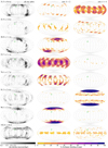 |
Fig. C.3. Fig. C.2 ctd. for longer periods of photometric data. |
| In the text | |
|
Fig. C.4. Example public folded G-band light curves for different period peaks, derived by the multi-harmonic modelling following a generalised least-squares period search as described in Sect. 4.1. The source id is provided in the top right corner. Additional information is available in Table 1 for sources with an asterisk. In general, the sources either have very high ripd, G, rexf, G, or aG significance (but always a low false-alarm probability). |
| In the text | |
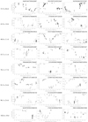 |
Fig. C.5. Fig. C.4 ctd. for longer periods of photometric data. |
| In the text | |
|
Fig. C.6. Ecliptic Aitoff projection of the astrometric period data presented in Fig. 24. Left: Source density of the astrometric peaks for the all-sky sample (top panel of Fig. 24). Right: Result of the all-sky uniform simulations of our noiseless sampled bias model (panels 2 and 3 of Fig. 24). They are colour-coded with the percentage of phases (position angles) that results in this peak: a low value means that only specific phasing of the scan-angle signal will result in a particular peak being observed at the given location. The green circle indicates the location of the GAPS catalogue. In all sky plots longitude zero is at the centre and increases to the left. |
| In the text | |
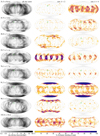 |
Fig. C.7. Fig. C.6 ctd. for longer periods of astrometric data. |
| In the text | |
|
Fig. D.1. Geometry of the scan across a source at S relative to the north celestial pole and north ecliptic pole, as viewed from outside the celestial sphere. |
| In the text | |
|
Fig. D.2. Histogram of ϕ for 106 random points of the sphere. |
| In the text | |
Current usage metrics show cumulative count of Article Views (full-text article views including HTML views, PDF and ePub downloads, according to the available data) and Abstracts Views on Vision4Press platform.
Data correspond to usage on the plateform after 2015. The current usage metrics is available 48-96 hours after online publication and is updated daily on week days.
Initial download of the metrics may take a while.