| Issue |
A&A
Volume 669, January 2023
|
|
|---|---|---|
| Article Number | A89 | |
| Number of page(s) | 14 | |
| Section | The Sun and the Heliosphere | |
| DOI | https://doi.org/10.1051/0004-6361/202244923 | |
| Published online | 16 January 2023 | |
Imaging individual active regions on the Sun’s far side with improved helioseismic holography
1
Max-Planck-Institut für Sonnensystemforschung, Justus-von-Liebig-Weg 3, 37077 Göttingen, Germany
e-mail: This email address is being protected from spambots. You need JavaScript enabled to view it.
2
Institut für Astrophysik, Georg-August-Universität Göttingen, Friedrich-Hund-Platz 1, 37077 Göttingen, Germany
3
Center for Space Science, NYUAD Institute, New York University Abu Dhabi, PO Box 129188 Abu Dhabi, UAE
4
Makutu, Inria, TotalEnergies, University of Pau, 64000 Pau, France
Received:
8
September
2022
Accepted:
8
November
2022
Abstract
Context. Helioseismic holography is a useful method for detecting active regions on the Sun’s far side and improving space weather forecasts.
Aims. We aim to improve helioseismic holography using a clear formulation of the problem, an accurate forward solver in the frequency domain, and a better understanding of the noise properties.
Methods. Building on the work of Lindsey et al. we define the forward- and backward-propagated wave fields (ingression and egression) in terms of a Green’s function. This Green’s function is computed using an accurate forward solver in the frequency domain. We analyse overlapping segments of 31 h of SDO/HMI dopplergrams, with a cadence of 24 h. Phase shifts between the ingression and the egression are measured and averaged to detect active regions on the far side.
Results. The phase maps are compared with direct extreme-ultraviolet (EUV) intensity maps from STEREO/EUVI. We confirm that medium-sized active regions can be detected on the far side with high confidence. Their evolution (and possible emergence) can be monitored on a daily time scale. Seismic maps averaged over 3 days provide an active-region detection rate as high as 75% and a false-discovery rate as low as 7% for active regions with areas above one thousandth of a hemisphere. For a large part, these improvements can be attributed to the use of a complete Green’s function (all skips) and the use of all available observations on the front side (full pupil).
Conclusions. Improved helioseismic holography enables the study of the evolution of medium-sized active regions on the Sun’s far side.
Key words: Sun: helioseismology / Sun: oscillations / Sun: activity / Sun: heliosphere
© The Authors 2023
 Open Access article, published by EDP Sciences, under the terms of the Creative Commons Attribution License (https://creativecommons.org/licenses/by/4.0), which permits unrestricted use, distribution, and reproduction in any medium, provided the original work is properly cited.
This article is published in open access under the Subscribe-to-Open model.
Open access funding provided by Max Planck Society.
1. Introduction
Detecting active regions on the far side of the Sun is potentially of great importance for space-weather forecasts (e.g., Arge et al. 2013; Hill 2018). Large active regions that emerge on the Sun’s far side will rotate into Earth’s view several days later; these may trigger coronal mass ejections (CMEs), which can damage satellites and spacecraft and endanger astronauts (e.g., Lindsey et al. 2011). It is known that far-side imaging can significantly improve models of the solar wind (Arge et al. 2013), which play an important role in space-weather forecasts.
Two approaches have been considered so far to monitor the far side of the Sun. The first solution consists of sending spacecraft to obtain a direct view of the far side. The two STEREO spacecrafts (in trailing and leading orbits) provided images of the Sun’s corona over the full range of S/C-Sun–Earth angles in the ecliptic plane (e.g., Howard et al. 2008). Solar Orbiter, now in operation, also provides direct images of the Sun from a sophisticated flight path out of the ecliptic, including magnetograms (Müller et al. 2020; Solanki et al. 2020). The other approach to imaging the far side of the Sun is helioseismology, using high-cadence data from the SDO spacecraft or the GONG ground-based network, for example. The concept of far-side helioseismology was unequivocally proven to work by Lindsey & Braun (2000b). This approach is admittedly challenging, but does not require the need to place additional spacecraft along nontrivial flight paths.
Acoustic waves propagate horizontally and are trapped in the vertical direction – they connect the Sun’s near and far sides. As acoustic waves travel faster in magnetized regions, they can inform us about the presence of active regions along their paths of propagation. Two helioseismic techniques, helioseismic holography (e.g., Lindsey & Braun 2000b, 2017; Braun & Lindsey 2002) and time–distance helioseismology (e.g., Zhao 2007; Ilonidis et al. 2009; Zhao et al. 2019) have been used to detect active regions on the far side. In the present article, we restrict our attention to helioseismic holography.
Far-side images computed using holography are publicly available. These include the JSOC/Stanford data set1and the NSO/GONG data set2. These data sets were validated by comparison with the STEREO/EUVI observations (Liewer et al. 2012, 2014, 2017) and maps of the magnetic field (González Hernández et al. 2007). Both pipelines use a delta function (single ray) representation of the Green’s function. While these far-side maps reveal large active regions on the far side, their quality is far from optimal. Several improvements have been proposed. For example, Pérez Hernández & González Hernández (2010) proposed the use of WKB approximations to the Green’s functions, and a combination of the two-skip and three-skip seismic wave paths. Felipe & Asensio Ramos (2019) used a machine-learning algorithm trained with Earth-side active regions to help detect small regions originally buried in noise (also see Broock et al. 2021).
The aim of this work is to improve holographic far-side images by taking advantage of recent theoretical and numerical advances in helioseismic imaging. In particular, we wish to work under the framework proposed by Gizon et al. (2018) to define signal and noise and we wish to use an accurate and efficient forward solver to compute the finite-wavelength Green’s functions (Gizon et al. 2017). We modify the JSOC/Stanford far-side imaging pipeline to include these updates. The resulting maps are then compared to the STEREO/EUVI observations when possible, and to other existing seismic maps.
2. Helioseismic holography
The basic steps of seismic holography are rather simple: (1) numerically propagate the observed wavefield on the Sun’s near side to target locations on the far side, (2) multiply the forward and backward propagated wavefields and measure a phase map, and then (3) subtract a reference measurement for the quiet Sun. These steps are described in detail in the following sections, and definitions are given for signal and noise.
2.1. Wave equation
Following Deubner & Gough (1984), we consider the scalar variable
 (1)
(1)
where ρ and c are the density and sound speed at position r, and ξ is the wave displacement vector at r and angular frequency ω. Ignoring terms involving gravity, this change of variable leads to a Helmholtz-like equation for ψ:
![Mathematical equation: $$ \begin{aligned} - \left[\nabla ^2 + k^2(\boldsymbol{r},\omega )\right] \psi (\boldsymbol{r},\omega ) = S(\boldsymbol{r},\omega ), \end{aligned} $$](/articles/aa/full_html/2023/01/aa44923-22/aa44923-22-eq2.gif) (2)
(2)
where k is the local wavenumber and
 (3)
(3)
In the frequency range of interest (2.5–4.5 mHz), we take the damping rate to be γ = γ0|ω/ω0|5.77, where γ0/2π = 4.29 μHz and ω0/2π = 3 mHz (Gizon et al. 2017). The quantity S in the above equation is a source term that represents wave excitation by turbulent convection. In writing the above equations, we assume the following Fourier convention:
 (4)
(4)
for any function of time f(t) that decays fast enough at infinity (±∞).
2.2. Wave propagators
The fundamental idea is to detect wave scattering by sunspots and other magnetic regions on the far side via the phase shift between the forward-propagated and the back-propagated wavefields (Lindsey & Braun 1997). At a given frequency ω, we define two integrals:
 (5)
(5)
where
![Mathematical equation: $$ \begin{aligned}&H_+ = - 2 \mathrm{i}\mathrm{Re}[k_n] G_0^*, \qquad \text{(egression} \text{ or} \text{ PB} \text{ integral),} \end{aligned} $$](/articles/aa/full_html/2023/01/aa44923-22/aa44923-22-eq6.gif) (6)
(6)
 (7)
(7)
and G0 is the causal Green’s function:
![Mathematical equation: $$ \begin{aligned} - \left[\nabla ^2 + k_0^2(\boldsymbol{r},\omega )\right] G_0(\boldsymbol{r},\boldsymbol{r}^{\prime }, \omega ) = \delta (\boldsymbol{r}-\boldsymbol{r}^{\prime }). \end{aligned} $$](/articles/aa/full_html/2023/01/aa44923-22/aa44923-22-eq8.gif) (8)
(8)
The wavenumber k0 is computed with Eq. (3) using the density ρ0(r) and sound-speed c0(r) from a 1D reference solar model (extended Model S, Fournier et al. 2017), and kn is the value of k0 at the computational boundary. Equation (8) is solved using the finite-element solver Montjoie (Duruflé 2006; Chabassier & Duruflé 2016; Gizon et al. 2017) with a radiation boundary condition applied 500 km above the solar surface (Gizon et al. 2018, Eq. (7)). The first integral, known as the egression, is an estimate of the back-propagated wavefield at the target location r. This definition, which differs from that of Lindsey & Braun (1997) by a multiplicative factor (and by the definition of the Green’s function), is based on the Porter-Bojarski integral used in the field of acoustics (PB integral, see Gizon et al. 2018, their Eq. (14)). The ingression is an estimate of the forward-propagated wavefield at the same location. Throughout this paper, the domain of integration, P, includes all the points from the center of the solar disk to angular distance 75°.
Figure 1 shows two example Green’s functions in the frequency range 2.5–4.5 mHz. The two-skip Green’s function used by the JSOC/Stanford far-side imaging pipeline (left panel) is computed under the ray-theory formalism of Lindsey & Braun (1997) and the corrections for dispersion described by Lindsey & Braun (2000a). The two-skip Green’s function is limited to separation distances in the range 115° < Δ < 172° and is used to image the far side to within a distance of 50° from the antipode of disk center (for a graphical representation of the 2 × 2 skip geometry, see Braun & Lindsey 2001). For distances from 50° to 90° from the antipode (the remaining part of the far side), a 3 × 1 skip geometry is used in the pipeline. The right panel of Fig. 1 shows the Green’s function obtained by solving Eq. (8) used under the formalism of Gizon et al. (2018). This particular Green’s function contains all spherical harmonics in the range 5 ≤ ℓ ≤ 45. It accounts for all skips, all distances, and finite wavelength effects. We refer the reader to Sect. 4.6 for a discussion about the consequences of the choice of Green’s function for imaging active regions on the far side.
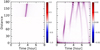 |
Fig. 1. Comparison between two choices of Green’s function used in helioseismic holography, as functions of the angular distance Δ between the source and the receiver (both on the solar surface) and time. In both cases, the frequency bandwidth is 2.5–4.5 mHz. Left panel: second-skip Green’s function based on the formalism of Lindsey & Braun (2000a; corrected ray theory) and used by the JSOC/Stanford far-side imaging pipeline. Distances from 115° to 172° are used to map the far side within 50° of the antipode to disk center. Right panel: Green’s function obtained by solving the scalar wave equation in the frequency domain (Eq. (8)). The solution is restricted to harmonic degrees in the range 5–45. |
2.3. Signal and noise
Due to the stochastic excitation of solar oscillations, the co-variance of the egression and the ingression, hereafter the holographic image intensity, is used in far-side imaging (Lindsey & Braun 2000b):
 (9)
(9)
In practice, holographic image intensities are averaged over a number of positive frequencies in the range 2.5–4.5 mHz to increase the signal-to-noise ratio (S/N):
 (10)
(10)
where N is the total number of frequencies (see Sect. 3).
In general, the quantity I is complex. We define the phase map as follows:
![Mathematical equation: $$ \begin{aligned} \Phi (\boldsymbol{r}) = \arg [ I (\boldsymbol{r}) / \langle I_{\rm 0}(\boldsymbol{r}) \rangle ] , \qquad \mathrm{(signal), } \end{aligned} $$](/articles/aa/full_html/2023/01/aa44923-22/aa44923-22-eq11.gif) (11)
(11)
where ⟨I0⟩ is a smooth reference, which is chosen to be the mean of the daily I over the quiet-Sun month of February 2019. The phase is computed with the routine angle from NumPy and takes values between −π and π. The level of realization noise is given by the standard deviation of the phase measured during the quiet-Sun period (using realizations with the same observation duration as for I; Gizon et al. 2018):
![Mathematical equation: $$ \begin{aligned} \sigma (\boldsymbol{r}) = \left( \mathrm{Var} \left[ \arg I_0 (\boldsymbol{r}) \right] \right)^{1/2} , \qquad \mathrm{(noise). } \end{aligned} $$](/articles/aa/full_html/2023/01/aa44923-22/aa44923-22-eq12.gif) (12)
(12)
The S/N is then equal to |Φ|/σ.
3. Data reduction
Helioseismology instruments do not provide us with direct access to the quantity ψ defined in Eq. (1). Instead, we may consider rough approximations of ψ, using either intensity images or Dopplergrams. Here we used full-disk Dopplergrams from SDO/HMI, each with 4096 × 4096 pixels and a spatial sampling of 0.5 arcsec and taken once every 45 s (Schou et al. 2012). Overlapping segments of 31 h were processed with a cadence of 24 h. The data set that we analyzed covers the period from May 1, 2010, to December 31, 2019. We first re-binned the individual Dopplergrams over 4 × 4 pixels, and subtracted a smooth fit. Each Dopplergram was divided by the sine of the angle between the local normal to the Sun’s surface and the line of sight in order to correct the amplitude variation due to projection. We then Postel projected each Dopplergram onto a grid with pixels separated by 0.002 rad (using bicubic interpolation). We obtained sets of 31h data cubes (2480 time steps) that track the Sun in the Carrington frame. The Dopplergrams were further binned by a factor of 8 along each spatial dimension, and were detrended at each pixel to remove the mean and the slope in time for each data cube. Values 5 sigma away from the mean (zero) were set to zero. The data cubes were transformed with respect to time using a fast Fourier transform. To circumvent the assumption of periodicity, the data sets were zero padded in time (4096 time steps), implying a frequency resolution of 5.425 μHz. A bandpass filter was applied to select frequencies in the range from 2.5 to 4.5 mHz.
4. Results
4.1. Example far-side maps
Figure 2 shows example composite maps of the solar surface in the Carrington frame for rotation CR 2147 in March 2014. In all four panels, we show the unsigned magnetic field Blos from SDO/HMI on the near side. Figure 2a shows the seismic phase Φ on the far side from one data segment of 31 h centered on March 4, 2014, using the improved wave propagators. The phase map captures the largest active regions that are also seen in the 304 Å STERERO/EUVI image on the same day on the far side (Fig. 2c), albeit with a rather low S/N. Figure 2b is similar to Fig. 2a, but the seismic phase on the far side is averaged over about three days. More precisely, we average I and I0 over three overlapping 31 h time segments centered respectively on March 3, 4, and 5, 2014; we compute Φ; and we filter out the small scales (spherical harmonic degrees l > 40). This 79 h averaged map (Fig. 2b) reveals the presence of relatively small active regions. By comparison, the 79 h averaged map from the JSOC/Stanford pipeline (Fig. 2d) appears to be more blurred.
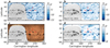 |
Fig. 2. Composite maps of the solar surface in the Carrington frame. In all panels, the near side (gray shades) shows the SDO/HMI unsigned line-of-sight magnetic field at 0:00 TAI on March 4, 2014. Panel a: far-side map using improved helioseismic holography (Φ, blue shades) applied to 31 h of SDO/HMI Dopplergrams centered on March 4, 2014. The red lines indicate the location of active region NOAA 12007 when it emerges ∼8 days later on the near side. The longitude is that of Carrington rotation 2147. Panel b: same as panel a but for a three-day average over March 3–5. A low pass spatial filter (l < 40) was applied. Panel c: far side seen by STEREO/EUVI at 304 Å. Panel d: far-side map from the standard JSOC/Stanford helioseismic pipeline (blue shades) using 3 days of data. |
Figure 3 shows the detection of a very large active region NOAA 12192 on both the near and far sides of the Sun. Figs. 3a and b are constructed the same way as in Figs. 2a and b, but for a daily map on September 29, 2014, and a three-day average over September 28–30. The large active region NOAA 12192 is clearly visible on the near side (red segments), whereas its signature is evidently captured by the phase map 13 days later on the far side (Figs. 3c and d).
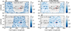 |
Fig. 3. Composite maps showing the very large active region NOAA 12192. Shown are composite maps, but for different Carrington rotations. STEREO observations are not available for comparison. Panels a,b: seismic map for September 29, 2014 (constructed as Fig. 2a) and the average over September 28–30 (constructed as Fig. 2b). The longitude is that of Carrington rotation 2155. Panels c,d: same as above, but 13 days later. Active region NOAA is very clearly seen on both the near and far sides. |
4.2. Active-region detection confidence levels
Figure 4 shows further details on how to distinguish active regions from the noisy background. Figures 4a and b show slices through the active region NOAA 12007 shown in the maps of Φ along the latitude marked by the red horizontal segments shown in Figs. 2a,b. The daily slices are plotted in Fig. 4a, and the averages over three days are shown in Fig. 4b. We clearly see the signature of this medium-size active region in the phase Φ, but there are fluctuations due to p-mode realization noise. The S/N improves when averaging over three days and filtering out the small spatial scales (see Fig. 4b).
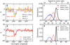 |
Fig. 4. Detection of active regions on the far side with helioseismic holography. Panel a: cuts through the phase maps of March 2014 at the latitude of active region NOAA 12007 (λ = 13.5°, see red horizontal lines in Fig. 2). The three curves correspond to March 3, 4, and 5. Panel b: the thick orange curve shows the phase when applying holography to three days at once (March 3–5). The purple curve is obtained after applying a spatial low-pass filter (l < 40). Panel c: the red curve shows the normalized distribution of the daily values of Φ in a disk of diameter 8° (∼100 Mm) centered on AR NOAA 12007 (see vertical dashed lines in panel a). In total, 14 days of data are used to track the region across the far side. The blue curve is the distribution for the very large region NOAA 12192 on October 2014 (see Fig. 3), constructed in the same way as for NOAA 12007. The black curve is the distribution of daily values in the quiet Sun, from which we measure the standard deviation of the noise, σ = 6.9°. Panel d: same as panel c, but the distributions are constructed from three-day spatially filtered maps of Φ, hence the smaller noise level σ = 2.3°. The threshold th = −3.5σ is plotted as a horizontal dashed line in panel b. We see that NOAA 12007 corresponds to a signal that is far beyond this threshold, with S/N ∼ 7. The very large active region NOAA 12192 is detected with a confidence level of nearly 100% (S/N ∼ 17). |
To quantify the detection confidence level, we show in Figs. 4c and d the distributions of the values of Φ within two active regions, NOAA 12007 and NOAA 12192 (a very large region), and we compare these distributions to the quiet Sun distributions (pure noise). The detection confidence level is high when there is little overlap between the distribution of values in an active region and the distribution corresponding to noise. For one day of data (Fig. 4c), we find that NOAA 12192 is detected with a confidence level of nearly 100%, while NOAA 12007 is detected with a S/N of about 2.5 (defining the S/N as the ratio between the mean of the active region distribution and the standard deviation of the noise; see the scale on the top axis of Fig. 4c). For three days of data (Fig. 4d), both active regions are detected with a confidence level of nearly 100% (S/Ns of 7 and 17). Therefore, time averaging and spatial filtering is an efficient means to improve the detection level of medium- and small-size active regions that do not evolve too fast.
4.3. Daily evolution of active regions on the far side
To follow the daily evolution of individual active regions from their emergence until they fade away, we cut slices at constant latitude through the maps in Fig. 2a. An example longitude–time map is shown in Fig. 5a, where daily slices with latitudes from 10° to 20° (in the north) are shown from the beginning of CR 2147 to the end of CR 2148. This map shows the evolution of individual active regions in this latitude range. In particular, we see that the active region NOAA 12007 emerges on the far side near the solar limb on February 26, 2014 (as indicated by the red arrow), grows in size into a bipolar active region, and starts to decay after it appears on the near side3. We also compare these seismic maps with STEREO/EUVI observations of the far side, and find that they show a very similar evolution of the active regions (see Figs. A.1 in the north and A.2 in the south). This demonstrates that seismic maps can be used not only to detect newly emerged regions on the far side, but also to characterize their evolution over consecutive days.
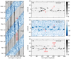 |
Fig. 5. Emergence of active regions on the far side. Panel a: longitude–time diagram extracted from the daily composite maps of Fig. 2a. Narrow bands in latitude (10° < λ < 20°) are stacked together to show the evolution of individual active regions. The blue shades correspond to the far side (daily seismic phase), and the gray shades to the near side (magnetograms, from CR 2147 to CR 2148). The red arrow indicates the time when active region NOAA 12007 emerges near the limb on the far side. Panels b–d: Carrington synoptic maps constructed by averaging the magnetograms on the near side (CR 2147 and 2148) and the seismic phase on the far side (CR 2147.5). At any spatial location, the data are averaged over 14 days in these Carrington maps. The red lines point to two particular active regions, NOAA 12007 and 12014, which are not visible in CR 2147 but visible in CR 2147.5 and 2148. |
4.4. Emergence of active regions on the far side
The right panels of Fig. 5 show three Carrington synoptic maps of the solar surface, which illustrate how to identify active regions that emerge on the far side. The top and bottom maps (Figs. 5b and d) are for Carrington rotations CR 2147 and CR 2148, respectively; they were constructed using line-of-sight magnetograms of the near side. The synoptic map in the middle (Fig. 5c) was constructed using the seismic phase on the far side and is denoted CR 2147.5. In each map, the value at a spatial location corresponds to a time average over approximately two weeks (see also, e.g., González Hernández et al. 2007). These three consecutive maps provide a picture of solar activity at times that are separated by approximately 13.5 days from one another (at fixed Carrington longitude).
Due to the long time averaging, active regions on the far side produce a sharp signature in the synoptic maps and are quite easy to distinguish from background noise. The spatial resolution is about twice the diffraction limit, or about 100 Mm. In the synoptic maps, we see a number of active regions at similar spatial locations on all three consecutive maps (Figs. 5b–d), which indicates their long lifetimes. Some other regions are not present on all three maps. For example, the two active regions highlighted by the red line segments in the figure are seen on the maps for CR 2147.5 and CR 2148, but they are not seen on the previous map CR 2147 (Fig. 5b). The active region in the north emerged on the far side (Fig. 5a) and can be identified later on the near side as active region NOAA 12007. The active region in the south emerges first near the limb as NOAA 11995, grows across the far side, and reappears on the near side as NOAA 12004 (Fig. A.2).
Synoptic maps from other Carrington rotations are shown in Fig. A.3, during both solar maximum and solar minimum. It is reassuring that the far-side maps show no false-positive detections during quiet times. This means in particular that far-side maps may provide important information for all-clear space weather predictions.
4.5. Comparisons to other seismic methods
STEREO observations of active regions on the far side have frequently been used as a reference to evaluate the validity of seismic images. We use STEREO/EUVI 304 Å maps of chromospheric emission remapped in a Carrington frame4 (averaged over 4 days) and we apply the thresholding method described by Liewer et al. (2017) to identify individual active regions on the far side. Example STEREO maps for October 2013 are shown in Fig. A.4a and the detected active regions as black regions in Fig. A.5a. The rectangular boxes around the detected active regions have areas proportional to the active region size.
In order to extract active regions from our seismic maps (three-day averages with Gaussian smoothing, Fig. A.4b), we apply a threshold to the phase Φ of th = −3.5 times the standard deviation σ = 0.045 rad = 2.6° measured from quiet-Sun maps. Following Lindsey & Braun (2017), we remove all detected regions that have an area S such that the integrated phase |∫SΦdS| is less than 30 rad per millionth of a hemisphere (1 ). Typically, this means that regions that are smaller than about 5 square degrees on the solar surface are removed. The results are shown in Fig. A.5b. The same algorithm (with th = −3σ, σ = 0.023 rad = 1.3°) is used to identify active regions from the JSOC/Stanford seismic holography “strong region maps” (five-day averages with Gaussian smoothing, Fig. A.4c) available online5. The corresponding active regions are shown in Fig. A.5c. For comparison, we also use the far-side maps obtained with time–distance helioseismology by Zhao et al. (2019). These maps are available online6 (four-day averages, [hmi.tdfsi12h] in the JSOC DRMS, see Fig. A.4d). Using the threshold in Φ of −0.06 rad proposed by Zhao et al. (2019) and removing the regions that contain no more than 10 pixels, we obtain the active regions shown in Fig. A.5d.
Assuming that the STEREO active regions represent the ground truth, we wish to assess the active-region detection rates for the three types of seismic map mentioned above. We consider an active-region detection to be a true detection if the active region detected with STEREO is also detected in a seismic map, that is, if the two active-region areas overlap. A detection is said to be false if an active region seen in a seismic map is not seen in the STEREO map, that is, if there is no overlap between active-region areas. We refer the reader to, for example, Ting (2010) and Benjamini & Hochberg (1995) for the definitions of true-positive and false-discovery rates.
Figure 6 shows the rates of true positives and false discoveries for the different seismic methods. The detection rates are applied to sets of active regions with areas above a certain value Smin. In total, 2.5 yr of data are used from January 1, 2012 to June 30, 2014, which corresponds to the period during which the two STEREO satellites observed a large fraction of the far side. We find that the JSOC/Stanford holography maps and the time–distance maps return very similar detection rates. The holography maps from this paper lead to a significantly higher true-positive detection rate and a significantly smaller false-discovery rate than the other two methods. For a minimum active region area of Smin = 1000 μhs, the true-positive rate reaches ∼75% and the false-discovery rate drops to ∼7%. This means that a proper calculation of the Green’s function is important in this problem.
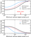 |
Fig. 6. Active-region detection statistics on the far side. The seismic maps from this work (three-day averages), the JSOC/Stanford seismic holography “strong region maps” (five-day averages), and the maps from time–distance helioseismology (Zhao et al. 2019, four-day averages) are compared with STEREO maps (four-day averages). Top panel: true-positive detection rates for the three seismic imaging methods as a function of minimum active region area Smin. The area of NOAA 12007 is S = 3.4 × 10³ μhs (red arrow and Fig. 2b). Bottom panel: false-discovery rates. The horizontal dashed line is drawn at 5%. Our improved method has a significantly smaller false-discovery rate than the other methods, in the Smin range of interest. |
Our choice of threshold, th = −3.5σ for three-day averages, can be justified a posteriori using a receiver operating characteristic (ROC) analysis (see, e.g., Flach et al. 2010). Figure 7 shows the true-positive rate versus the false-discovery rate for several values of the threshold th from −5σ to −2σ, while fixing the minimum active region area to Smin = 1000 μhs. We see that all values of th give a significantly better outcome than a purely random detection method (black dashed line with slope 1). The optimal threshold lies between th = −3.5σ and th = −3σ, where the distance to the diagonal (corresponding to a purely random detection method) is the largest in the ROC diagram.
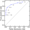 |
Fig. 7. ROC analysis: True positive rate versus false discovery rate for different thresholds in Φ (th). Our improved far-side maps (three-day averages) are used and the minimum active-region area is fixed at Smin = 1000 μhs. Random detections would fall on the black dashed line. For all thresholds th, the outcome is clearly above this diagonal. The optimal threshold, th = −3.5σ, corresponds to the point that is farthest from the diagonal. It is reported as a horizontal dashed line in Fig. 4b. |
4.6. Where does the improvement come from?
We show that the Green’s function that solves Eq. (8) leads to a significant improvement in helioseismic far-side imaging. This Green’s function differs from the simplified Green’s function used by Lindsey & Braun (2000a) in several ways (see Fig. 1): (i) all branches (all skips) are kept, (ii) all separation distances are kept, and (iii) the details of the solution in each particular branch differ (at least for the second skip). In order to investigate the contribution of these differences to the improvement, we apply several truncations to our Green’s function and compare the results to those of the JSOC/Stanford pipeline.
First, we keep only the second skip part of the Green’s function (for the branch with the shortest path) and we truncate the separation distances as in the JSOC/Stanford pipeline (115° < Δ < 172°). The resulting S/N of the active regions in the helioseismic maps is shown in the second column of Fig. 8 for two particular active regions. The improvement is only ∼10%, implying that the wave-based Green’s function is not significantly different from the ray-based function (once corrected using the “local control correlation”, see Lindsey & Braun 2000a).
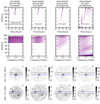 |
Fig. 8. Green’s functions and associated S/Ns of the phase maps of the far side. Top row: Green’s functions in the time–distance domain. Second row: imaginary part of Green’s functions in the frequency–distance domain. Third row: S/N for active region NOAA 12192 averaged over October 9–11, 2014. Last row: S/Ns for active region NOAA 12007 averaged over March 3–5, 2014. Panels a,e: maps using the ray-based Green’s function from the JSOC/Stanford pipeline, for focus points within 50° of the far-side disk center. Panels b,f: maps using the wave-based Green’s function restricted to the second-skip and separation distances 115°−172°. The map covers 60° within the far-side disk center. Panels c,g: same as panels b and f, but without truncating the Green’s function in separation distance. Panels d,h: same as panels c and g, but using all branches of the wave-based Green’s function, which is the approach used in the present paper. In panels a–h, the black solid lines mark the equator. The blue lines indicate locations of active regions NOAA 12192 (third row) and NOAA 12007 (last row). |
In a second step, we study the consequences of using all separation distances while keeping the second skip only. The corresponding S/Ns are shown in the third column of Fig. 8. We see that filling out the hole in the observation pupil leads to better focusing on the far side. The S/N increases by ∼10% when including all available data in the analysis (see the changes from Figs. 8b and f to Figs. 8c and g).
In a third step, we look at the relative improvement brought by letting through the other branches of the Green’s function (Fig. 8, top right panel). The corresponding changes are seen in the transition from Figs. 8c and g to Figs. 8d and h. The additional branches of the Green’s function clearly lead to the most significant improvement in S/N, at a level of 50%–100% depending on the active region.
A concise view of the three successive improvements is presented in Fig. A.6. Cuts through the active regions in the seismic maps (phases) confirm that the improvement is mostly due to the use of all the branches in the Green’s function and the use of a full observation pupil (all the available data are used as input).
5. Conclusion
We demonstrate that the spatial resolution and the S/N of helioseismic holography maps of the far side of the Sun improve when accurate propagators are used in the analysis. Here we used the finite-wavelength Green’s function computed in the frequency domain by Gizon et al. (2017), and the transparent boundary conditions determined by Fournier et al. (2017) and Barucq et al. (2018). In particular, we find that a spatial resolution of order 100 Mm can be reached, i.e. twice the size of a sunspot.
When it comes to the detection of active regions, we show in Sect. 4.5 that seismic maps averaged over three days provide a detection rate as high as ∼75% and a false-discovery rate as small as ∼7% for a minimum active region area Smin = 1000 μhs. The outcome depends sensitively on the threshold th used to identify active regions in the phase maps, as illustrated by the ROC diagram (Fig. 7). Given that the false-discovery rate is very small – which can also be verified during quiet-Sun periods – the far-side maps should be most helpful to forecast all-clear space weather conditions (see, e.g., Hill 2018).
We also show that seismic maps can be used to track the emergence and evolution of individual active regions on a daily basis as they move across the far side. This conclusion was reached using STEREO chromospheric images as a reference. The upcoming photospheric observations of the far side of the Sun by the Polarimetric and Helioseismic Imager on Solar Orbiter (Solanki et al. 2020) should provide definitive confirmation of the accuracy of far-side helioseismic holography.
We refer the reader to the time-distance helioseismology results of Zhao et al. (2019, their Fig. 9), where active region NOAA 12007 is detected in two-day averages around March 6, 2014.
Acknowledgments
We are very grateful to Charles Lindsey (NWRA/CoRA) for providing access to his helioseismic holography code and very helpful discussions. We thank Damien Fournier (MPS) for his help with the computation of the Green’s functions. We also thank an anonymous referee for constructive comments. L.G. and D.Y. acknowledge funding from the ERC Synergy Grant WHOLE SUN (#810218) and the DFG Collaborative Research Center SFB 1456 (project C04). LG acknowledges NYUAD Institute Grant G1502. H.B. acknowledges funding from the 2021-0048: Geothermica SEE4GEO of European project and the associated team program ANTS of Inria. The HMI data are courtesy of SDO (NASA) and the HMI consortium. The SDO/HMI holographic far-side images are computed and maintained by JSOC/Stanford at http://jsoc.stanford.edu/data/farside/. The SDO/HMI time-distance far-side images are made available at http://jsoc.stanford.edu/data/timed/. The EUVI maps are generated by the SECCHI team and maintained at JHUAPL, in collaboration with NRL and JPL.
References
- Arge, C. N., Henney, C. J., Hernandez, I. G., et al. 2013, AIP Conf. Ser., 1539, 11 [NASA ADS] [Google Scholar]
- Barucq, H., Chabassier, J., Duruflé, M., Gizon, L., & Leguèbe, M. 2018, ESAIM: Math. Modell. Numer. Anal., 52, 945 [CrossRef] [EDP Sciences] [Google Scholar]
- Benjamini, Y., & Hochberg, Y. 1995, J. Roy. Stat. Soc., Ser. B (Method.), 57, 289 [Google Scholar]
- Braun, D. C., & Lindsey, C. 2001, ApJ, 560, L189 [NASA ADS] [CrossRef] [Google Scholar]
- Braun, D. C., & Lindsey, C. 2002, AAS Meeting Abstracts, 200, 89.06 [NASA ADS] [Google Scholar]
- Broock, E. G., Felipe, T., & Asensio Ramos, A. 2021, A&A, 652, A132 [NASA ADS] [CrossRef] [EDP Sciences] [Google Scholar]
- Chabassier, J., & Duruflé, M. 2016, High order finite element method for solving convected helmholtz equation in radial and axisymmetric domains: application to helioseismology (Inria Bordeaux Sud-Ouest), Research Report RR-8893, https://hal.inria.fr/hal-01295077 [Google Scholar]
- Deubner, F.-L., & Gough, D. 1984, ARA&A, 22, 593 [NASA ADS] [CrossRef] [Google Scholar]
- Duruflé, M. 2006, Ph.D. Thesis, ENSTA ParisTech, France [Google Scholar]
- Felipe, T., & Asensio Ramos, A. 2019, A&A, 632, A82 [NASA ADS] [CrossRef] [EDP Sciences] [Google Scholar]
- Flach, P. A. 2010, in ROC Analysis, eds. C. Sammut, & G. I. Webb (Boston, MA: Springer, US), 869 [Google Scholar]
- Fournier, D., Leguèbe, M., Hanson, C. S., et al. 2017, A&A, 608, A109 [CrossRef] [EDP Sciences] [Google Scholar]
- Gizon, L., Barucq, H., Duruflé, M., et al. 2017, A&A, 600, A35 [NASA ADS] [CrossRef] [EDP Sciences] [Google Scholar]
- Gizon, L., Fournier, D., Yang, D., Birch, A. C., & Barucq, H. 2018, A&A, 620, A136 [NASA ADS] [CrossRef] [EDP Sciences] [Google Scholar]
- González Hernández, I., Hill, F., & Lindsey, C. 2007, ApJ, 669, 1382 [CrossRef] [Google Scholar]
- Hill, F. 2018, Space Weather, 16, 1488 [NASA ADS] [CrossRef] [Google Scholar]
- Howard, R. A., Moses, J. D., Vourlidas, A., et al. 2008, Space Sci. Rev., 136, 67 [NASA ADS] [CrossRef] [Google Scholar]
- Ilonidis, S., Zhao, J., & Hartlep, T. 2009, Sol. Phys., 258, 181 [NASA ADS] [CrossRef] [Google Scholar]
- Liewer, P. C., González Hernández, I., Hall, J. R., Thompson, W. T., & Misrak, A. 2012, Sol. Phys., 281, 3 [NASA ADS] [Google Scholar]
- Liewer, P. C., González Hernández, I., Hall, J. R., Lindsey, C., & Lin, X. 2014, Sol. Phys., 289, 3617 [NASA ADS] [CrossRef] [Google Scholar]
- Liewer, P. C., Qiu, J., & Lindsey, C. 2017, Sol. Phys., 292, 146 [NASA ADS] [CrossRef] [Google Scholar]
- Lindsey, C., & Braun, D. C. 1997, ApJ, 485, 895 [NASA ADS] [CrossRef] [Google Scholar]
- Lindsey, C., & Braun, D. C. 2000a, Science, 287, 1799 [Google Scholar]
- Lindsey, C., & Braun, D. C. 2000b, Sol. Phys., 192, 261 [Google Scholar]
- Lindsey, C., & Braun, D. C. 2017, Space Weather, 15, 761 [NASA ADS] [CrossRef] [Google Scholar]
- Lindsey, C., Braun, D., Hernández, I. G., & Donea, A. 2011, in Holography - Different Fields of Application, ed. F. A. Monroy Ramíre (London: IntechOpen) [Google Scholar]
- Müller, D., St. Cyr, O. C., Zouganelis, I., et al. 2020, A&A, 642, A1 [Google Scholar]
- Pérez Hernández, F., & González Hernández, I. 2010, ApJ, 711, 853 [CrossRef] [Google Scholar]
- Schou, J., Scherrer, P. H., Bush, R. I., et al. 2012, Sol. Phys., 275, 229 [Google Scholar]
- Solanki, S. K., del Toro Iniesta, J. C., Woch, J., et al. 2020, A&A, 642, A11 [NASA ADS] [CrossRef] [EDP Sciences] [Google Scholar]
- Ting, K. M. 2010, in Sensitivity and Specificity, eds. C. Sammut, & G. I. Webb (Boston: Springer), 901 [Google Scholar]
- Zhao, J. 2007, ApJ, 664, L139 [NASA ADS] [CrossRef] [Google Scholar]
- Zhao, J., Hing, D., Chen, R., & Hess Webber, S. 2019, ApJ, 887, 216 [NASA ADS] [CrossRef] [Google Scholar]
Appendix A: Additional figures
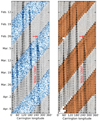 |
Fig. A.1. Longitude-time diagrams extracted from the daily composite maps for latitude bands in the north (15° ±5°). Left panel: The far-side maps are obtained from seismology and shown in blue (same as Fig. 2a). Right panel: The far-side maps are obtained from STEREO/EUVI and shown in orange. The red arrow marks the time when active region NOAA 12007 emerges. |
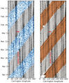 |
Fig. A.2. Same as Fig. A.1, but for latitude bands in the south (−15° ±5°). The red arrow marks the time when active region NOAA 11995 emerges (called 12014 one rotation later). |
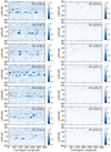 |
Fig. A.3. Seismic synoptic maps of the far side constructed as in Fig. 4c. Left panels: Carrington rotations 2144.5–2150.5 during the maximum phase of Cycle 24 (2013–2014). Right panels: Carrington rotations 2218.5–2224.5 during solar minimum in 2019. The same color scale is used for all maps. |
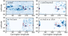 |
Fig. A.4. Detections of far-side active regions on October 15, 2013 (12:00 TAI). Panel (a): Composite EUV maps at 304 Åfrom Liewer et al. (2017; four-day averages). The detected active regions are enclosed in the red boxes. Panel (b): Seismic far-side images from this work (three-day averages). For reference, the red boxes are copied from panel (a). Panel (c): Same as panel b but for holographic far-side maps from JSOC/Stanford (five-day averages). Panel (d): Same as panel b but for time–distance far-side maps from Zhao et al. (2019; four-day averages). |
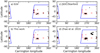 |
Fig. A.5. Detected active regions in each of the four panels of Fig. A.4 (black regions). For reference, the red boxes are copied from Fig. A.4a (EUV map). Latitudes above 60° are ignored (cf. blue contours). Such data are used to generate the true positive detection rates and the false-discovery rates discussed in Sect. 4.5. |
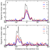 |
Fig. A.6. Signal-to-noise ratios from Fig. 8 plotted along horizontal cuts through the active regions NOAA 12192 (panel (i), see blue horizontal lines in Figs. 8a–d) and NOAA 12007 (panel (ii), see blue horizontal lines in Figs. 8e–h). |
All Figures
|
Fig. 1. Comparison between two choices of Green’s function used in helioseismic holography, as functions of the angular distance Δ between the source and the receiver (both on the solar surface) and time. In both cases, the frequency bandwidth is 2.5–4.5 mHz. Left panel: second-skip Green’s function based on the formalism of Lindsey & Braun (2000a; corrected ray theory) and used by the JSOC/Stanford far-side imaging pipeline. Distances from 115° to 172° are used to map the far side within 50° of the antipode to disk center. Right panel: Green’s function obtained by solving the scalar wave equation in the frequency domain (Eq. (8)). The solution is restricted to harmonic degrees in the range 5–45. |
| In the text | |
|
Fig. 2. Composite maps of the solar surface in the Carrington frame. In all panels, the near side (gray shades) shows the SDO/HMI unsigned line-of-sight magnetic field at 0:00 TAI on March 4, 2014. Panel a: far-side map using improved helioseismic holography (Φ, blue shades) applied to 31 h of SDO/HMI Dopplergrams centered on March 4, 2014. The red lines indicate the location of active region NOAA 12007 when it emerges ∼8 days later on the near side. The longitude is that of Carrington rotation 2147. Panel b: same as panel a but for a three-day average over March 3–5. A low pass spatial filter (l < 40) was applied. Panel c: far side seen by STEREO/EUVI at 304 Å. Panel d: far-side map from the standard JSOC/Stanford helioseismic pipeline (blue shades) using 3 days of data. |
| In the text | |
|
Fig. 3. Composite maps showing the very large active region NOAA 12192. Shown are composite maps, but for different Carrington rotations. STEREO observations are not available for comparison. Panels a,b: seismic map for September 29, 2014 (constructed as Fig. 2a) and the average over September 28–30 (constructed as Fig. 2b). The longitude is that of Carrington rotation 2155. Panels c,d: same as above, but 13 days later. Active region NOAA is very clearly seen on both the near and far sides. |
| In the text | |
|
Fig. 4. Detection of active regions on the far side with helioseismic holography. Panel a: cuts through the phase maps of March 2014 at the latitude of active region NOAA 12007 (λ = 13.5°, see red horizontal lines in Fig. 2). The three curves correspond to March 3, 4, and 5. Panel b: the thick orange curve shows the phase when applying holography to three days at once (March 3–5). The purple curve is obtained after applying a spatial low-pass filter (l < 40). Panel c: the red curve shows the normalized distribution of the daily values of Φ in a disk of diameter 8° (∼100 Mm) centered on AR NOAA 12007 (see vertical dashed lines in panel a). In total, 14 days of data are used to track the region across the far side. The blue curve is the distribution for the very large region NOAA 12192 on October 2014 (see Fig. 3), constructed in the same way as for NOAA 12007. The black curve is the distribution of daily values in the quiet Sun, from which we measure the standard deviation of the noise, σ = 6.9°. Panel d: same as panel c, but the distributions are constructed from three-day spatially filtered maps of Φ, hence the smaller noise level σ = 2.3°. The threshold th = −3.5σ is plotted as a horizontal dashed line in panel b. We see that NOAA 12007 corresponds to a signal that is far beyond this threshold, with S/N ∼ 7. The very large active region NOAA 12192 is detected with a confidence level of nearly 100% (S/N ∼ 17). |
| In the text | |
|
Fig. 5. Emergence of active regions on the far side. Panel a: longitude–time diagram extracted from the daily composite maps of Fig. 2a. Narrow bands in latitude (10° < λ < 20°) are stacked together to show the evolution of individual active regions. The blue shades correspond to the far side (daily seismic phase), and the gray shades to the near side (magnetograms, from CR 2147 to CR 2148). The red arrow indicates the time when active region NOAA 12007 emerges near the limb on the far side. Panels b–d: Carrington synoptic maps constructed by averaging the magnetograms on the near side (CR 2147 and 2148) and the seismic phase on the far side (CR 2147.5). At any spatial location, the data are averaged over 14 days in these Carrington maps. The red lines point to two particular active regions, NOAA 12007 and 12014, which are not visible in CR 2147 but visible in CR 2147.5 and 2148. |
| In the text | |
|
Fig. 6. Active-region detection statistics on the far side. The seismic maps from this work (three-day averages), the JSOC/Stanford seismic holography “strong region maps” (five-day averages), and the maps from time–distance helioseismology (Zhao et al. 2019, four-day averages) are compared with STEREO maps (four-day averages). Top panel: true-positive detection rates for the three seismic imaging methods as a function of minimum active region area Smin. The area of NOAA 12007 is S = 3.4 × 10³ μhs (red arrow and Fig. 2b). Bottom panel: false-discovery rates. The horizontal dashed line is drawn at 5%. Our improved method has a significantly smaller false-discovery rate than the other methods, in the Smin range of interest. |
| In the text | |
|
Fig. 7. ROC analysis: True positive rate versus false discovery rate for different thresholds in Φ (th). Our improved far-side maps (three-day averages) are used and the minimum active-region area is fixed at Smin = 1000 μhs. Random detections would fall on the black dashed line. For all thresholds th, the outcome is clearly above this diagonal. The optimal threshold, th = −3.5σ, corresponds to the point that is farthest from the diagonal. It is reported as a horizontal dashed line in Fig. 4b. |
| In the text | |
|
Fig. 8. Green’s functions and associated S/Ns of the phase maps of the far side. Top row: Green’s functions in the time–distance domain. Second row: imaginary part of Green’s functions in the frequency–distance domain. Third row: S/N for active region NOAA 12192 averaged over October 9–11, 2014. Last row: S/Ns for active region NOAA 12007 averaged over March 3–5, 2014. Panels a,e: maps using the ray-based Green’s function from the JSOC/Stanford pipeline, for focus points within 50° of the far-side disk center. Panels b,f: maps using the wave-based Green’s function restricted to the second-skip and separation distances 115°−172°. The map covers 60° within the far-side disk center. Panels c,g: same as panels b and f, but without truncating the Green’s function in separation distance. Panels d,h: same as panels c and g, but using all branches of the wave-based Green’s function, which is the approach used in the present paper. In panels a–h, the black solid lines mark the equator. The blue lines indicate locations of active regions NOAA 12192 (third row) and NOAA 12007 (last row). |
| In the text | |
|
Fig. A.1. Longitude-time diagrams extracted from the daily composite maps for latitude bands in the north (15° ±5°). Left panel: The far-side maps are obtained from seismology and shown in blue (same as Fig. 2a). Right panel: The far-side maps are obtained from STEREO/EUVI and shown in orange. The red arrow marks the time when active region NOAA 12007 emerges. |
| In the text | |
|
Fig. A.2. Same as Fig. A.1, but for latitude bands in the south (−15° ±5°). The red arrow marks the time when active region NOAA 11995 emerges (called 12014 one rotation later). |
| In the text | |
|
Fig. A.3. Seismic synoptic maps of the far side constructed as in Fig. 4c. Left panels: Carrington rotations 2144.5–2150.5 during the maximum phase of Cycle 24 (2013–2014). Right panels: Carrington rotations 2218.5–2224.5 during solar minimum in 2019. The same color scale is used for all maps. |
| In the text | |
|
Fig. A.4. Detections of far-side active regions on October 15, 2013 (12:00 TAI). Panel (a): Composite EUV maps at 304 Åfrom Liewer et al. (2017; four-day averages). The detected active regions are enclosed in the red boxes. Panel (b): Seismic far-side images from this work (three-day averages). For reference, the red boxes are copied from panel (a). Panel (c): Same as panel b but for holographic far-side maps from JSOC/Stanford (five-day averages). Panel (d): Same as panel b but for time–distance far-side maps from Zhao et al. (2019; four-day averages). |
| In the text | |
|
Fig. A.5. Detected active regions in each of the four panels of Fig. A.4 (black regions). For reference, the red boxes are copied from Fig. A.4a (EUV map). Latitudes above 60° are ignored (cf. blue contours). Such data are used to generate the true positive detection rates and the false-discovery rates discussed in Sect. 4.5. |
| In the text | |
|
Fig. A.6. Signal-to-noise ratios from Fig. 8 plotted along horizontal cuts through the active regions NOAA 12192 (panel (i), see blue horizontal lines in Figs. 8a–d) and NOAA 12007 (panel (ii), see blue horizontal lines in Figs. 8e–h). |
| In the text | |
Current usage metrics show cumulative count of Article Views (full-text article views including HTML views, PDF and ePub downloads, according to the available data) and Abstracts Views on Vision4Press platform.
Data correspond to usage on the plateform after 2015. The current usage metrics is available 48-96 hours after online publication and is updated daily on week days.
Initial download of the metrics may take a while.