| Issue |
A&A
Volume 674, June 2023
Solar Orbiter First Results (Nominal Mission Phase)
|
|
|---|---|---|
| Article Number | A183 | |
| Number of page(s) | 9 | |
| Section | The Sun and the Heliosphere | |
| DOI | https://doi.org/10.1051/0004-6361/202346030 | |
| Published online | 19 June 2023 | |
Direct assessment of SDO/HMI helioseismology of active regions on the Sun’s far side using SO/PHI magnetograms
1
Max-Planck-Institut für Sonnensystemforschung, Justus-von-Liebig-Weg 3, 37077 Göttingen, Germany
e-mail: This email address is being protected from spambots. You need JavaScript enabled to view it.
, This email address is being protected from spambots. You need JavaScript enabled to view it.
2
Institut für Astrophysik, Georg-August-Universität Göttingen, Friedrich-Hund-Platz 1, 37077 Göttingen, Germany
3
Center for Space Science, NYUAD Institute, New York University Abu Dhabi, PO Box 129188 Abu Dhabi, UAE
4
Makutu, Inria, TotalEnergies, University of Pau, 64000 Pau, France
5
Instituto de Astrofísica de Andalucía (IAA-CSIC), Apartado de Correos 3004, 18080 Granada, Spain
6
Univ. Paris-Sud, Institut d’Astrophysique Spatiale, UMR 8617, CNRS, Bâtiment 121, 91405 Orsay Cedex, France
7
Instituto Nacional de Técnica Aeroespacial, Carretera de Ajalvir, km 4, 28850 Torrejón de Ardoz, Spain
8
Universitat de València, Catedrático José Beltrán 2, 46980 Paterna-Valencia, Spain
9
Leibniz-Institut für Sonnenphysik, Schöneckstr. 6, 79104 Freiburg, Germany
10
Instituto Universitario “Ignacio da Riva”, Universidad Politécnica de Madrid, IDR/UPM, Plaza Cardenal Cisneros 3, 28040 Madrid, Spain
11
University of Barcelona, Department of Electronics, Carrer de Martí i Franquès, 1–11, 08028 Barcelona, Spain
12
Institut für Datentechnik und Kommunikationsnetze der TU Braunschweig, Hans-Sommer-Str. 66, 38106 Braunschweig, Germany
13
Fraunhofer Institute for High-Speed Dynamics, Ernst-Mach-Institut, EMI, Ernst-Zermelo-Str. 4, 79104 Freiburg, Germany
Received:
30
January
2023
Accepted:
27
April
2023
Abstract
Context. Earth-side observations of solar p modes can be used to image and monitor magnetic activity on the Sun’s far side. In this work, we use magnetograms of the far side obtained by the Polarimetric and Helioseismic Imager (PHI) on board Solar Orbiter (SO) to directly assess the validity of far-side helioseismic holography for the first time.
Aims. We wish to co-locate the positions of active regions in helioseismic images and magnetograms and to calibrate the helioseismic measurements in terms of the magnetic field strength.
Methods. We identified three magnetograms displaying a total of six active regions on the far side from 18 November 2020, 3 October 2021, and 3 February 2022. The first two dates are from the SO cruise phase and the third is from the beginning of the nominal operation phase. We computed contemporaneous seismic phase maps for these three dates using helioseismic holography applied to the time series of Dopplergrams from the Helioseismic and Magnetic Imager (HMI) at the Solar Dynamics Observatory (SDO).
Results. Among the six active regions seen in SO/PHI magnetograms, five of them are identified on the seismic maps at almost the same positions as on the magnetograms. One region is too weak to be detected above the seismic noise. To calibrate the seismic maps, we fit a linear relationship between the seismic phase shifts and the unsigned line-of-sight magnetic field averaged over the active region areas extracted from the SO/PHI magnetograms.
Conclusions. SO/PHI provides the strongest evidence so far that helioseismic imaging is able to provide reliable information on active regions on the far side, including their positions, areas, and the mean unsigned magnetic field.
Key words: Sun: helioseismology / Sun: photosphere / Sun: magnetic fields / Sun: activity
© The Authors 2023
 Open Access article, published by EDP Sciences, under the terms of the Creative Commons Attribution License (https://creativecommons.org/licenses/by/4.0), which permits unrestricted use, distribution, and reproduction in any medium, provided the original work is properly cited.
This article is published in open access under the Subscribe to Open model.
Open access funding provided by Max Planck Society.
1. Introduction
The solar surface provides important boundary conditions for the extrapolation of the structure and evolution of the global magnetic field into the heliosphere, where it interacts with the Earth’s magnetosphere (see, e.g., review by Owens & Forsyth 2013, and references therein). Half of the solar surface is invisible from an Earth vantage point, which leads to sizable uncertainties when modeling the heliospheric field and limits the accuracy of space weather forecasts (Arge et al. 2013; Cash et al. 2015; Wallace et al. 2022; Jain et al. 2022). This missing part of the solar surface, often referred to as the Sun’s far side, is accessible to spacecraft with large Earth-Sun-S/C angles, such as the Solar Terrestrial Relations Observatory (STEREO) and Solar Orbiter. The two STEREO spacecraft see the solar corona in the extreme ultraviolet (EUV) spectrum (Howard et al. 2008), while Solar Orbiter observes the corona, along with all the photospheric observables: intensity, Doppler velocity, and vector magnetic field (Müller et al. 2020; Solanki et al. 2020).
The Sun’s far side is also accessible to helioseismic holography (see, e.g., Lindsey & Braun 2000; Braun & Lindsey 2002), which provides information about magnetic activity in the solar near-surface layers. The input data for helioseismology consist of observations of solar acoustic oscillations from either the ground-based Global Oscillations Network Group (GONG; Harvey et al. 1996) or the Solar Dynamics Observatory (SDO; Pesnell et al. 2012) in geosynchronous orbit. This technique has been partially validated using far-side images of the chromosphere from STEREO/EUVI (Liewer et al. 2012, 2014, 2017) or photospheric magnetograms that are shifted in time to wait for active regions to come into Earth’s view (González Hernández et al. 2007). In addition to helioseismic holography, time–distance helioseismology has also been used to detect active regions on the far side and has been partially validated using STEREO chromospheric images (e.g., Zhao 2007; Zhao et al. 2019). Such a validation can only be partial since, in the first case, coronal images are not perfectly representative of the photospheric magnetic field and, in the second case, active regions evolve over daily and weekly time scales. Thanks to recent advances in computational helioseismology (Gizon et al. 2017), the detection rate of the active regions on the Sun’s far side has improved significantly: STEREO data indicate that most of the medium-sized active regions can be detected with confidence with helioseismic holography (Yang et al. 2023).
In order to be included in models of the heliospheric field or space weather, the seismic measurements need to be calibrated with respect to the photospheric magnetic field (see a preliminary attempt by Arge et al. 2013). Such calibrations have been considered on the front side using simultaneous SOHO/MDI line-of-sight magnetograms (Braun & Lindsey 2001; Lindsey & Braun 2005a,b) and on the far side using (two-week delayed) GONG synoptic magnetograms (González Hernández et al. 2007) as well as STEREO-based proxies of the unsigned photospheric magnetic field (Chen et al. 2022). However, the optimal observations needed to calibrate far-side helioseismology are contemporaneous images of the photospheric magnetic field, which were not available until the advent of Solar Orbiter (SO). The Polarimetric and Helioseismic Imager (PHI) on board SO provided line-of-sight magnetograms of the far side during the cruise and the early science phase of the mission (Solanki et al. 2020). In this paper, we aim to use these direct magnetic field measurements to assess and calibrate seismic images on the Sun’s far side using the recent improvements in helioseismic holography reported by Yang et al. (2023).
2. Observations
2.1. SO/PHI magnetograms showing far-side active regions
We use the magnetograms from the SO/PHI-Full Disk Telescope (FDT), which measures the Stokes parameters of the Fe I 6173 Å spectral line at six wavelength positions (Solanki et al. 2020). During the cruise phase, SO/PHI was only switched on occasionally within the so-called “remote-sensing checkout windows” during which it provided at most a few magnetograms per day (Zouganelis et al. 2020). Daily magnetograms covering several months of observations on the far side will be made available relatively soon; however, this data set is still undergoing processing and is not included in this work. A multi-view synoptic map for a single Carrington rotation was processed by Löschl et al. (2023). The SO/PHI raw data can be reduced and processed either on board (Albert et al. 2020) or on the ground. The on-ground data processed includes additional corrections (fringe and ghost corrections).
The present work uses SO/PHI-FDT magnetograms, each with 2048 × 2048 pixels, but with a varying spatial sampling of the solar disk due to a large range of Sun-S/C distances (highest resolution at disk center of ≈730 km reached at 0.28 au; see Solanki et al. 2020). In total, three magnetograms are analyzed, corresponding to the specific times when SO/PHI saw active regions on the far side. These data are from the cruise phase on 18 November 2020 and 3 October 2021 (processed on board) and from the nominal science phase on 3 February 2022 (processed on-ground). At the time of writing, the magnetograms have been reduced in a preliminary manner only and consequently are affected by large-scale imperfections across the field of view (different for each image). We estimate these systematics by fitting a low-order polynomial of the form  to the data using a least squares method, where x and y are the pixel coordinates and the fit applies only to the pixels that are outside of active regions. Example raw and processed magnetograms (after subtraction of the large-scale systematics) are shown in Fig. 1.
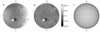 |
Fig. 1. SO/PHI-FDT observations of the Sun’s far side on 18 November 2020 during Solar Orbiter’s cruise phase. Panel a: line-of-sight magnetic field, Blos. Panel b: corrected Blos after removing the large-scale systematics by fitting a low-order polynomial (see Sect. 2.1). Panel c: continuum intensity, I. In each panel, the black dashed curve marks the solar equator and the orange dash curves highlight the latitude bands 25° ≤λ ≤ 40° in the north and −30° ≤λ ≤ −15° in the south. |
2.2. Helioseismic maps
We applied far-side helioseismic holography to series of Dopplergrams from the Helioseismic and Magnetic Imager (HMI; Schou et al. 2012) on board SDO. The data reduction process directly follows the steps described in detail by Yang et al. (2023). Helioseismic holography measures the phase shift Φ between the ingression and the egression, namely, between the forward- and the backward-propagated acoustic waves from the observed surface to any target location on the Sun’s far side. The acoustic waves propagate faster in magnetized regions on the surface, which will cause a negative shift in Φ. The maps of Φ can be used to detect individual active regions on the far side and to monitor their evolution (Yang et al. 2023).
Following Yang et al. (2023), we used seismic phase maps averaged over 79 h. These phase maps are given in Carrington coordinates (during CR 2237, 2249, and 2253) and are smoothed with a Gaussian kernel of full width 4° to remove the spatial scales smaller than half the typical wavelength on the surface of the seismic waves used in the analysis. The far-side maps centered on 18 November 2020 (Fig. 2b) and 3 October 2021 (Fig. A.1b) were computed during periods when the duty cycle of SDO/HMI Dopplergrams was almost 100%. The third phase map centered on 3 February 2022 was computed during the eclipse season of SDO (24 January–17 February 2022), a period of lower quality images and lower duty cycle (94%, 92%, and 77% on February 2, 3, and 4 2022). The lower data rate on February 4 is mainly due to snow on the receiving antenna dish. This explains the higher seismic noise for the 79-h average phase map centered on 3 February 2022 (Fig. A.1d).
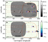 |
Fig. 2. Magnetic activity on the entire solar surface on 18 November 2020 during Carrington Rotation CR 2237. Panel a: SO/PHI-FDT magnetogram covers a large fraction of the far side, while a 3-day averaged SDO/HMI magnetogram shows magnetic activity on the near side. Four active regions identified on the far side by SO/PHI are outlined by red contours (see Table 1). Panel b: green-blue shades show the helioseismic phase Φ on the far side, deduced from acoustic oscillations observed on the near-side by SDO/HMI over 79 h between 17–19 November. The seismic phase is shown over a range corresponding to 1.5 − 6 times the standard deviation of the noise in the quiet Sun (σΦ = 2.6°). |
3. Direct assessment of helioseismic imaging
Figure 2a shows the SO/PHI line-of-sight magnetograms on 18 November 2020, which includes several active regions on the far side marked by red contours. The other two magnetograms are shown in Figs. A.1a,c. In total, we identified six far-side active regions in the collection of SO/PHI magnetograms that were available to us, including five relatively big regions and a much smaller region. The parameters of these far-side active regions are given in Table 1. Tracking these regions on the far side makes it possible to assign to each of them a NOAA number as they rotate onto the front side. Figures 2b, A.1b,d show the values of the seismic phase over a range corresponding to 1.5 − 6 times the standard deviation of the noise in the quiet Sun (σΦ = 2.6°). The five largest active regions observed by SO/PHI are clearly visible in the contemporaneous helioseismic phase maps, at almost the same positions and with similar areas as seen on the magnetograms.
Far-side active regions seen by SO/PHI.
Figure 3a shows the positions of the active regions determined from the seismic maps with respect to their true positions measured from the SO/PHI magnetograms. These positions are obtained by computing the center of gravity of the data over the corresponding active region areas. For the SO/PHI data, the active region areas are defined as the areas with magnetic field above 20 G from the unsigned magnetograms smoothed by a Gaussian kernel of width 4°. For the helioseismic data, we first identified the active regions using a detection threshold of −3.5σΦ (as proposed by Yang et al. 2023, see green curves in Fig. A.2) and then extended the active region areas using a lower threshold of −2σΦ (see blue curves in Fig. A.2). Only the data within SO/PHI’s field of view were used in the analysis. As shown in Fig. 3a, all five active regions detected in the seismic maps are within a few degrees of their true positions. This remarkable result is consistent with the resolution limit of seismic imaging (half the typical acoustic wavelength at the surface corresponds to an angular distance of approximately 4°).
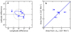 |
Fig. 3. Positions of active regions 1, 2, 4, 5, and 6 deduced from the seismic maps, with respect to their actual positions deduced from the SO/PHI magnetograms (a). The active region coordinates are computed using a center-of-gravity method, applied to each observable (Φ or Blos) within the region areas. For the SO/PHI magnetograms, the active region areas correspond to the red contours in Figs. 2 and A.1 (20 G contours from the smoothed magnetograms). For the helioseismic data, a threshold of 2σΦ is used to determine the active region areas. The blue ellipse shows the probability density function of the data points at half maximum, assuming a bivariate normal distribution. The dashed circle with a diameter 4° corresponds to the resolution limit of the seismic observations. Active region areas inferred from helioseismology versus areas measured from the SO/PHI magnetograms (b). The linear fit gives a slope of 0.98 (solid blue line). The dashed line is the 1:1 diagonal. |
Figure 3b shows that the helioseismically-determined areas of the active regions (2σΦ threshold) are similar to the true areas determined from the SO/PHI magnetic field data. While this result is encouraging, a definitive statement would require the analysis of a much larger data set. It is useful to measure active-region areas on the far side, for example, to obtain solar irradiance computations (and predictions) from various vantage points.
These aspects demonstrate that far-side helioseismic holography works well. The seismic phase shifts associated with the active regions may then be empirically related to magnetic field strength measured by SO/PHI. For the small active region in the South in Fig. 2 (active region 3), no excess signal is seen in the seismic phase maps.
4. Preliminary calibration of seismic maps
We compute the values of |Blos| and Φ averaged over the areas of the six active regions detected on the far side and outlined by the red contours (e.g., in Fig. 2) extracted from the SO/PHI-FDT magnetograms. These spatial averages over active region areas are denoted with angle brackets ⟨ ⋅ ⟩AR. As shown in Fig. 4, the data suggest a trend where ⟨Φ⟩AR decreases with ⟨|Blos|⟩AR (i.e., while increasing in absolute value).
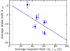 |
Fig. 4. Helioseismic phase shift Φ versus unsigned line-of-sight magnetic field |Blos|, both averaged over each of the six active regions on the far side (blue dots). Active region areas are determined from SO/PHI magnetograms (red contours in Figs. 2 and A.1). The numerical values are provided in Table 1 and the error bars refer to ±1σΦ seismic noise. The blue solid line is a linear fit with slope −0.2 deg G−1 and intercept (5 G, 0°). |
With only six data points, the exact functional relationship between the two quantities is difficult to determine. Once the zero point is fixed, we find that a linear fit is as good as a quadratic fit to describe the data (reduced χ2 of 11.1 versus 11.0). For the linear fit we obtain:
 (1)
(1)
where the quiet Sun reference |Blos|≈5 G is measured near solar minimum (see also Korpi-Lagg et al. 2022). We note that the scatter of the data points in Fig. 4 could potentially be reduced by taking into account the positions of active regions with respect to disk center in both maps. We intend to study this possibility in the future when many more active regions will be available from the SO/PHI synoptic program. Figure A.3 shows plots of the seismic phase calibrated using the transformation:
 (2)
(2)
The quantity BΦ can be understood as a seismic estimate of the unsigned magnetic field |Blos|. In Fig. A.3, both BΦ and |Blos| were averaged over the latitude bands shown in Figs. 2a,b for active region 2 (panel a) and active regions 1 and 4 (panel b) on 18 November 2020. BΦ matches reasonably well with |Blos| observed by SO/PHI for all three active regions in terms of position and shapes. With the proposed calibration, we find very similar amplitudes for BΦ and |Blos| for active regions 1 and 4 (Fig. A.3b), while a factor of two difference is seen for active region 2 (Fig. A.3a).
5. Emergence and evolution of active regions
With STEREO chromospheric images, Yang et al. (2023) showed that seismic phase maps can be used to study the evolution of active regions on the far side. By applying the scaling relation Eq. (2) to the seismic phase maps and by combining them with front side magnetograms, we can follow the evolution of active regions over multiple rotations in a consistent manner. Such a longitude-time plot combining BΦ and |Blos| is shown in Fig. 5 for the period from 23 October to 26 December 2020, where active regions NOAA 12787 (in the north), 12781/90, and 12786 (in the south) can be followed. The magnetic proxy BΦ is shown in the range 20 − 50 G on the far side, while the Earth side shows |Blos| from SDO/HMI in the same range. |Blos| from SO/PHI-FDT (orange) is shown for the date of 18 November 2020. Figure 5 gives a consistent view for the evolution of the active regions from their emergence until they disperse. In particular, we see clearly that NOAA 12781 and 12 790 refer to the same active region. Active region NOAA 12781 is shown to emerge on 28 October 2020, growing until it comes into Earth’s view, and then starts to disperse. This region later rotates on the far side, reappears on the near side as NOAA 12790, and then fades away with a total life of ≈45 days. Thus, far-side imaging (validated with SO/PHI) enables us to measure the time of emergence of active regions and to track long-lived regions across multiple Carrington rotations. Another representation of the evolution of this active region is given by Fig. A.4.
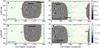 |
Fig. 5. Longitude–time diagrams based on subsets of maps such as Fig. 2b. Left panel: latitude bands in the northern hemisphere (25° ≤λ ≤ 40°, see Fig. 2) stacked in time to cover the period from 23 October to 26 December 2020. The far side shows calibrated phase maps, BΦ, in the range of 20 − 50 G (blue shades). The near side shows the unsigned line-of-sight magnetic field Blos from SDO/HMI (gray shades) in the same range. The unsigned Blos from SO/PHI-FDT for 18 November 2020 is shown in orange. Right panel: same as the left panel but for latitude bands in the southern hemisphere (−30° ≤λ ≤ −15°, see Fig. 2). The red star indicates the occurrence of an M 4.4 class flare near the limb on 29 November 2020, associated with NOAA 12790. |
6. Conclusion
In this work, we have shown how the SO/PHI magnetograms are key to validating far-side helioseismic imaging. We find that the few active regions identified on the far side are located in seismic maps at almost the same positions and with similar areas as in the SO/PHI line-of-sight magnetograms. Furthermore, the seismic phase associated with an active region can be empirically related to the average unsigned magnetic field. This work gives the strongest evidence so far that seismic imaging – as implemented by Gizon et al. (2018) and Yang et al. (2023) – provides reliable information about active regions on the Sun’s far side. This calibration is not yet perfect since only the line-of-sight component of the field is available (at the time of writing) and we only considered six active regions in three magnetograms. Once this approach is extended to the many more far-side active regions to be observed by SO/PHI, we will be able to improve the calibration of the seismic maps. This will lead to an improved understanding of the emergence and evolution of active regions over the entire solar surface.
Acknowledgments
We thank an anonymous referee for their thoughtful comments. D.Y. and L.G. acknowledge funding from ERC Synergy Grant WHOLE SUN (#810218) and Deutsche Forschungsgemeinschaft (DFG) Collaborative Research Center SFB 1456 (#432680300, project C04). L.G. acknowledges NYUAD Institute Grant G1502. H.B. acknowledges funding from the 2021–0048: Geothermica SEE4GEO of European project and the associated team program ANTS of Inria. The HMI data are courtesy of SDO (NASA) and the HMI consortium. Solar Orbiter is a space mission of international collaboration between ESA and NASA, operated by ESA. We are grateful to the ESA SOC and MOC teams for their support. The German contribution to SO/PHI is funded by the BMWi through DLR and by MPG central funds. The Spanish contribution is funded by AEI/MCIN/10.13039/501100011033/(RTI2018-096886-C5, PID2021-125325OB-C5, PCI2022-135009-2) and ERDF “A way of making Europe”, Center of Excellence Severo Ochoa Awards to IAA-CSIC (SEV-2017-0709, CEX2021-001131-S), and a Ramón y Cajal fellowship to DOS. The French contribution is funded by CNES.
References
- Albert, K., Hirzberger, J., Kolleck, M., et al. 2020, J. Astron. Telesc. Instrum. Syst., 6, 048004 [NASA ADS] [CrossRef] [Google Scholar]
- Arge, C. N., Henney, C. J., Hernandez, I. G., et al. 2013, AIP Conf. Ser., 1539, 11 [NASA ADS] [Google Scholar]
- Braun, D. C., & Lindsey, C. 2001, ApJ, 560, L189 [NASA ADS] [CrossRef] [Google Scholar]
- Braun, D. C., & Lindsey, C. 2002, The First Seismic Images of the Solar Interior and Far Side from the GONG+ Network, https://www.cora.nwra.com/~dbraun/farside-gong/ [Google Scholar]
- Cash, M. D., Biesecker, D. A., Pizzo, V., et al. 2015, Space Weather, 13, 611 [CrossRef] [Google Scholar]
- Chen, R., Zhao, J., Hess Webber, S., et al. 2022, ApJ, 941, 197 [NASA ADS] [CrossRef] [Google Scholar]
- Gizon, L., Barucq, H., Duruflé, M., et al. 2017, A&A, 600, A35 [NASA ADS] [CrossRef] [EDP Sciences] [Google Scholar]
- Gizon, L., Fournier, D., Yang, D., Birch, A. C., & Barucq, H. 2018, A&A, 620, A136 [NASA ADS] [CrossRef] [EDP Sciences] [Google Scholar]
- González Hernández, I., Hill, F., & Lindsey, C. 2007, ApJ, 669, 1382 [CrossRef] [Google Scholar]
- Harvey, J. W., Hill, F., Hubbard, R. P., et al. 1996, Science, 272, 1284 [Google Scholar]
- Howard, R. A., Moses, J. D., Vourlidas, A., et al. 2008, Space Sci. Rev., 136, 67 [NASA ADS] [CrossRef] [Google Scholar]
- Jain, K., Lindsey, C., Adamson, E., et al. 2022, ArXiv e-prints [arXiv:2210.01291] [Google Scholar]
- Korpi-Lagg, M. J., Korpi-Lagg, A., Olspert, N., & Truong, H. L. 2022, A&A, 665, A141 [NASA ADS] [CrossRef] [EDP Sciences] [Google Scholar]
- Liewer, P. C., González Hernández, I., Hall, J. R., Thompson, W. T., & Misrak, A. 2012, Sol. Phys., 281, 3 [NASA ADS] [Google Scholar]
- Liewer, P. C., González Hernández, I., Hall, J. R., Lindsey, C., & Lin, X. 2014, Sol. Phys., 289, 3617 [NASA ADS] [CrossRef] [Google Scholar]
- Liewer, P. C., Qiu, J., & Lindsey, C. 2017, Sol. Phys., 292, 146 [NASA ADS] [CrossRef] [Google Scholar]
- Lindsey, C., & Braun, D. C. 2000, Science, 287, 1799 [Google Scholar]
- Lindsey, C., & Braun, D. C. 2005a, ApJ, 620, 1107 [NASA ADS] [CrossRef] [Google Scholar]
- Lindsey, C., & Braun, D. C. 2005b, ApJ, 620, 1118 [CrossRef] [Google Scholar]
- Löschl, P., Valori, G., Hirzberger, J., et al. 2023, A&A, submitted [Google Scholar]
- Müller, D., St Cyr, O. C., Zouganelis, I., et al. 2020, A&A, 642, A1 [Google Scholar]
- Owens, M. J., & Forsyth, R. J. 2013, Liv. Rev. Sol. Phys., 10, 5 [Google Scholar]
- Pesnell, W. D., Thompson, B. J., & Chamberlin, P. C. 2012, Sol. Phys., 275, 3 [Google Scholar]
- Schou, J., Scherrer, P. H., Bush, R. I., et al. 2012, Sol. Phys., 275, 229 [Google Scholar]
- Solanki, S. K., del Toro Iniesta, J. C., Woch, J., et al. 2020, A&A, 642, A11 [NASA ADS] [CrossRef] [EDP Sciences] [Google Scholar]
- Wallace, S., Jones, S. I., Arge, C. N., Viall, N. M., & Henney, C. J. 2022, ApJ, 935, 24 [NASA ADS] [CrossRef] [Google Scholar]
- Yang, D., Gizon, L., & Barucq, H. 2023, A&A, 669, A89 [NASA ADS] [CrossRef] [EDP Sciences] [Google Scholar]
- Zhao, J. 2007, ApJ, 664, L139 [NASA ADS] [CrossRef] [Google Scholar]
- Zhao, J., Hing, D., Chen, R., & Hess Webber, S. 2019, ApJ, 887, 216 [NASA ADS] [CrossRef] [Google Scholar]
- Zouganelis, I., De Groof, A., Walsh, A. P., et al. 2020, A&A, 642, A3 [NASA ADS] [CrossRef] [EDP Sciences] [Google Scholar]
Appendix A: Additional figures
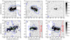 |
Fig. A.1. Same as Fig. 2, but for the other two active regions identified with SO/PHI on the far side (red contours): Active region 5 on 3 October 2021 (left panels) and active region 6 (right panels) on 3 February 2022. Both regions appear on the near side about one day later. The higher seismic noise in the right panels is due to lower-quality SDO/HMI data (see main text). |
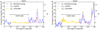 |
Fig. A.2. Contour plots of the helioseismic phase overlaid on SO/PHI unsigned magnetograms (gray scale saturated at 50 G) for far-side active regions 1 to 6 (see labels in top-left corners). The black dashed contours correspond to |Blos| = 20 G after Gaussian smoothing. The blue, green, and purple contours correspond to Φ = −2σΦ, −3.5σΦ, and −5σΦ, respectively. The red curves mark the boundaries between the far and Earth sides. Active region 3 is not detected by helioseismology. |
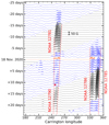 |
Fig. A.3. Plots of BΦ from far-side helioseismology for 17–19 November 2020 (blue) and unsigned line-of-sight magnetic field |Blos| on 18 November 2020 from SO/PHI (orange) and SDO/HMI (yellow). The data are averaged over the latitude band 25° ≤λ ≤ 40° in the north (a) and over the latitude band −30° ≤λ ≤ −15° in the south (b). Note: |Blos| is smoothed in longitude with a running mean over 4°. The active regions 1, 2, and 4 are indicated on the plots (see Table 1). Notice that the values shown here for active regions 1, 2, and 4 are not directly comparable to the values given in Fig. 4 because we are averaging over latitude bands and not over active region areas. |
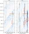 |
Fig. A.4. Average of the data from the right panel of Fig. 5 over the latitudinal band −30° ≤λ ≤ −15° in the South. The averages of BΦ are given by the blue curves (far side), the averages of |Blos| by the black curves (near side), and the average of |Blos| from SO/PHI for 18 November 2020 by the orange curve. The magnetic field data are further smoothed in longitude with a running mean over 4°. The filled areas below the curves highlight the values above 20 G. The red star indicates the same flare (M 4.4), as shown in Fig. 5. |
All Tables
All Figures
|
Fig. 1. SO/PHI-FDT observations of the Sun’s far side on 18 November 2020 during Solar Orbiter’s cruise phase. Panel a: line-of-sight magnetic field, Blos. Panel b: corrected Blos after removing the large-scale systematics by fitting a low-order polynomial (see Sect. 2.1). Panel c: continuum intensity, I. In each panel, the black dashed curve marks the solar equator and the orange dash curves highlight the latitude bands 25° ≤λ ≤ 40° in the north and −30° ≤λ ≤ −15° in the south. |
| In the text | |
|
Fig. 2. Magnetic activity on the entire solar surface on 18 November 2020 during Carrington Rotation CR 2237. Panel a: SO/PHI-FDT magnetogram covers a large fraction of the far side, while a 3-day averaged SDO/HMI magnetogram shows magnetic activity on the near side. Four active regions identified on the far side by SO/PHI are outlined by red contours (see Table 1). Panel b: green-blue shades show the helioseismic phase Φ on the far side, deduced from acoustic oscillations observed on the near-side by SDO/HMI over 79 h between 17–19 November. The seismic phase is shown over a range corresponding to 1.5 − 6 times the standard deviation of the noise in the quiet Sun (σΦ = 2.6°). |
| In the text | |
|
Fig. 3. Positions of active regions 1, 2, 4, 5, and 6 deduced from the seismic maps, with respect to their actual positions deduced from the SO/PHI magnetograms (a). The active region coordinates are computed using a center-of-gravity method, applied to each observable (Φ or Blos) within the region areas. For the SO/PHI magnetograms, the active region areas correspond to the red contours in Figs. 2 and A.1 (20 G contours from the smoothed magnetograms). For the helioseismic data, a threshold of 2σΦ is used to determine the active region areas. The blue ellipse shows the probability density function of the data points at half maximum, assuming a bivariate normal distribution. The dashed circle with a diameter 4° corresponds to the resolution limit of the seismic observations. Active region areas inferred from helioseismology versus areas measured from the SO/PHI magnetograms (b). The linear fit gives a slope of 0.98 (solid blue line). The dashed line is the 1:1 diagonal. |
| In the text | |
|
Fig. 4. Helioseismic phase shift Φ versus unsigned line-of-sight magnetic field |Blos|, both averaged over each of the six active regions on the far side (blue dots). Active region areas are determined from SO/PHI magnetograms (red contours in Figs. 2 and A.1). The numerical values are provided in Table 1 and the error bars refer to ±1σΦ seismic noise. The blue solid line is a linear fit with slope −0.2 deg G−1 and intercept (5 G, 0°). |
| In the text | |
|
Fig. 5. Longitude–time diagrams based on subsets of maps such as Fig. 2b. Left panel: latitude bands in the northern hemisphere (25° ≤λ ≤ 40°, see Fig. 2) stacked in time to cover the period from 23 October to 26 December 2020. The far side shows calibrated phase maps, BΦ, in the range of 20 − 50 G (blue shades). The near side shows the unsigned line-of-sight magnetic field Blos from SDO/HMI (gray shades) in the same range. The unsigned Blos from SO/PHI-FDT for 18 November 2020 is shown in orange. Right panel: same as the left panel but for latitude bands in the southern hemisphere (−30° ≤λ ≤ −15°, see Fig. 2). The red star indicates the occurrence of an M 4.4 class flare near the limb on 29 November 2020, associated with NOAA 12790. |
| In the text | |
|
Fig. A.1. Same as Fig. 2, but for the other two active regions identified with SO/PHI on the far side (red contours): Active region 5 on 3 October 2021 (left panels) and active region 6 (right panels) on 3 February 2022. Both regions appear on the near side about one day later. The higher seismic noise in the right panels is due to lower-quality SDO/HMI data (see main text). |
| In the text | |
|
Fig. A.2. Contour plots of the helioseismic phase overlaid on SO/PHI unsigned magnetograms (gray scale saturated at 50 G) for far-side active regions 1 to 6 (see labels in top-left corners). The black dashed contours correspond to |Blos| = 20 G after Gaussian smoothing. The blue, green, and purple contours correspond to Φ = −2σΦ, −3.5σΦ, and −5σΦ, respectively. The red curves mark the boundaries between the far and Earth sides. Active region 3 is not detected by helioseismology. |
| In the text | |
|
Fig. A.3. Plots of BΦ from far-side helioseismology for 17–19 November 2020 (blue) and unsigned line-of-sight magnetic field |Blos| on 18 November 2020 from SO/PHI (orange) and SDO/HMI (yellow). The data are averaged over the latitude band 25° ≤λ ≤ 40° in the north (a) and over the latitude band −30° ≤λ ≤ −15° in the south (b). Note: |Blos| is smoothed in longitude with a running mean over 4°. The active regions 1, 2, and 4 are indicated on the plots (see Table 1). Notice that the values shown here for active regions 1, 2, and 4 are not directly comparable to the values given in Fig. 4 because we are averaging over latitude bands and not over active region areas. |
| In the text | |
|
Fig. A.4. Average of the data from the right panel of Fig. 5 over the latitudinal band −30° ≤λ ≤ −15° in the South. The averages of BΦ are given by the blue curves (far side), the averages of |Blos| by the black curves (near side), and the average of |Blos| from SO/PHI for 18 November 2020 by the orange curve. The magnetic field data are further smoothed in longitude with a running mean over 4°. The filled areas below the curves highlight the values above 20 G. The red star indicates the same flare (M 4.4), as shown in Fig. 5. |
| In the text | |
Current usage metrics show cumulative count of Article Views (full-text article views including HTML views, PDF and ePub downloads, according to the available data) and Abstracts Views on Vision4Press platform.
Data correspond to usage on the plateform after 2015. The current usage metrics is available 48-96 hours after online publication and is updated daily on week days.
Initial download of the metrics may take a while.