| Issue |
A&A
Volume 692, December 2024
|
|
|---|---|---|
| Article Number | A182 | |
| Number of page(s) | 11 | |
| Section | The Sun and the Heliosphere | |
| DOI | https://doi.org/10.1051/0004-6361/202451625 | |
| Published online | 12 December 2024 | |
The return of FarNet-II: Generation of solar far-side magnetograms from helioseismic data
1
Instituto de Astrofísica de Canarias, 38205 C/Vía Láctea, s/n, La Laguna, Tenerife, Spain
2
Departamento de Astrofísica, Universidad de La Laguna, 38205 La Laguna, Tenerife, Spain
⋆ Corresponding author; This email address is being protected from spambots. You need JavaScript enabled to view it.
Received:
23
July
2024
Accepted:
3
October
2024
Abstract
Context. The far-side activity of the Sun can be inferred by interpreting the near-side wave field using local helioseismic techniques. However, detections are limited to strongly active regions because signal-to-noise ratio of the data is low. Recently, we developed the FarNet and FarNet-II neural networks to improve the identification of active regions on far-side seismic maps.
Aims. We aim to use FarNet-II to leverage seismic data to infer far-side magnetograms, including the magnetic field strength and polarity.
Methods. We used FarNet-II to produce sequences of 11 consecutive binned magnetograms with a 12-hour cadence of a central section of the far side, where each pixel was assigned to one of nine possible classes that define its magnetic field and polarity. The inputs to the network are sequences of phase-shift maps of the same regions, computed using helioseismic holography. We trained the network using a cross-validation approach to estimate its reliability. The targets for the training and the cross-validation were obtained from near-side Helioseismic and Magnetic Imager magnetograms, taken half a rotation later than the seismic data. The metric we used for the evaluation is the volumetric Dice, a newly defined metric that measures the overlap between the outputs and the targets. The results were compared with Solar Orbiter data from a period with far-side coverage between May 2022 and September 2022.
Results. FarNet-II achieves an average volumetric Dice of 0.249, showing a good visual superposition between the targets and outputs of the network. The comparisons of the outputs and the Solar Orbiter magnetograms are also similar.
Conclusions. FarNet-II can correctly predict the level of activity and the polarity of far-side regions using near-side seismic data. This capability can be leveraged in space-weather forecasting.
Key words: Sun: activity / Sun: helioseismology / Sun: oscillations / sunspots
© The Authors 2024
 Open Access article, published by EDP Sciences, under the terms of the Creative Commons Attribution License (https://creativecommons.org/licenses/by/4.0), which permits unrestricted use, distribution, and reproduction in any medium, provided the original work is properly cited.
This article is published in open access under the Subscribe to Open model. This email address is being protected from spambots. You need JavaScript enabled to view it. to support open access publication.
1. Introduction
Solar magnetic activity is the source of multiple phenomena that might affect technological and biological systems on Earth and its surrounding space. Space weather is the branch of astrophysics that is dedicated to studying the state of the Sun and interplanetary space in the Solar System to predict these potentially hazardous events and to help us prepare in advance. The knowledge of the solar magnetism in the whole Sun, and not only the visible hemisphere, is essential for an accurate forecast of space weather. This has two fundamental reasons. First, active regions can be precursors of large coronal mass ejections or other highly energetic events. These events could impact the Earth, even if they occur just after the active region rotates into the near-side hemisphere. Monitoring the solar far side is fundamental to addressing whether an active region can be considered potentially threatening to our technological devices. Second, the accuracy of the predictions of several space-weather parameters, such as solar irradiance or the solar wind speed, which are forecast regularly, benefit from taking the activity on the far side into account (Arge et al. 2013; Fontenla et al. 2009).
The only method that currently allows a continuous monitoring of the solar far side is far-side helioseismology. Helioseismology is a field of solar physics that uses the waves that are trapped inside the Sun to probe the solar interior. The study of the global oscillation eigenmodes is commonly known as global helioseismology. Even though it has been an important tool that provided insight into the internal structure and the dynamics of our star (Christensen-Dalsgaard 2002), it is only able to study global properties. To study local structures in the solar interior, local helioseismology techniques (Braun et al. 1987, 1992; Hill 1988; Duvall et al. 1993) are needed. Local helioseismology analyzes the whole wave field, not just the eigenfrequencies. Helioseismic holography (Lindsey & Braun 2000a) is a local helioseismology method that is based on the regression of acoustic p modes. It uses the wave field of a region of the surface, called “pupil”, to infer the properties of acoustically connected locations below the surface, called “focal points”. One of the techniques in helioseismic holography is phase-sensitive holography (Braun & Lindsey 2000). This technique integrates ideas of optical interferometry into the study of the solar interior (Lindsey & Braun 2000b). This technique can detect wave scatterers below the surface by computing two quantities: the ingression, which represents the driving term of acoustic waves traveling from the pupil to the focal point, and the egression, which is the time-reversed counterpart of ingression. Then, the correlation of the two is computed to detect a potential phase shift caused by magnetic structures in the focal point.
One of the most successful applications of phase-sensitive holography is far-side imaging (Lindsey & Braun 1990). It was first used by Lindsey & Braun (2000a). The technique leverages the transparency of the solar interior to waves of certain frequencies that propagate through the Sun in a bouncing manner because they are refracted in deep layers and reflected on the surface. Active regions have a depressed surface, the Wilson depression, because their magnetic field is strong. When acoustic waves from deep layers are reflected on the surface of an active region, they are reflected at a lower depth than the waves that arrive at the quiet Sun. This shortens the wave path. This shortening causes most of the phase shift that is detected when the waves return to the near side (Lindsey et al. 2010; Schunker et al. 2013; Felipe et al. 2017). Since the gas pressure increases exponentially with depth, the seismic signal is proportional to the logarithm of the magnetic pressure, that is, to the logarithm of the squared magnetic field strength. The relation between the magnetic field strength and the seismic signatures of far-side active regions was empirically calibrated by González Hernández et al. (2007), who compared the far-side seismic signal with the magnetic flux of the active regions after they appeared in the near hemisphere. This calibration was confirmed by MacDonald et al. (2015) using near-side data, that is, simultaneous measurements of the helioseismic phase shift and magnetic field. They also proved that the tilt and area of the active regions seen in magnetograms are consistent with their seismic counterpart. These works suggested that the seismic signal is a reliable insight based on which we can infer the size, orientation, and magnetic field strength of active regions. In contrast, the inference of the polarity of the active regions poses a challenge because the seismic signal does not contain information about it. Previous studies have employed Hale’s law to assign the polarity of an active region (Arge et al. 2013). Still, most methods that are routinely in use today do not infer the far-side magnetic field magnitude, just the presence or absence of activity in each region.
Far-side imaging achieved through phase-sensitive holography, while giving very promising results for large active regions on the far side, is not able to detect smaller and fainter activity because of the low signal-to-noise ratio of the data (González Hernández et al. 2007; Liewer et al. 2014, 2017). Felipe & Asensio Ramos (2019) developed the neural network FarNet to improve the detection of solar activity on the far side using phase-shift data. It follows a standard encoder-decoder U-net architecture (Ronneberger et al. 2015) and uses convolutional layers, batch normalization (BN; Ioffe & Szegedy 2015), and rectified linear units (ReLU; Nair & Hinton 2010). The encoder reduces the spatial size of the input while increasing the number of channels, using max-pooling (Goodfellow et al. 2016), and the decoder increases the spatial size while decreasing the number of channels, using transposed convolutions (Zeiler et al. 2010). It also uses skip connections, as does the standard U-net in Ronneberger et al. (2015), to leverage information of encoder layers on decoder operations. This accelerates the training while avoiding vanishing gradients. Broock et al. (2021) evaluated the network using an extensive dataset. They confirmed the improvement over the helioseismic standard method. Later, Broock et al. (2022) developed FarNet-II, an improved version of FarNet, which was proven to provide a significantly better performance than FarNet in the detection of far-side activity. All these methods, as we commented earlier, only infer the presence or absence of activity, and not the magnitude of the magnetic field.
Over the past decades, the seismic monitoring of the far side, and methods whose goal is to enhance detections using seismic monitoring as a basis, have proven to be reliable tools for detecting and locating active regions in the nonvisible hemisphere. However, the implementation of these detections in models to forecast the heliosphere requires not only the inference of the position of the active regions, but also their field strength and polarity. Recently, Chen et al. (2022) generated an algorithm to predict far-side unsigned magnetism from helioseismic maps, based on the idea that was proven by González Hernández et al. (2007) that the seismis signal contains information about the magnetic field magnitude. They followed the following strategy to obtain the magnetograms employed for the training. First, a neural network was trained to compute the far-side magnetic flux from Extreme Ultraviolet (EUV) data from the Atmospheric Imaging Assembly (AIA; Lemen et al. 2012) on board the Solar Dynamics Observatory (SDO). Then, this network was applied to far-side EUV observations from the Solar Terrestrial Relations Observatory (STEREO; Kaiser 2004), producing synthetic far-side magnetic flux maps. This approach is similar to the approach developed by Kim et al. (2019), but neglects the sign of the magnetic field. The synthetic magnetic flux maps were finally used as the target in another neural network that estimates far-side magnetic flux maps from time-distance seismic data (Duvall & Kosovichev 2001; Zhao 2007; Ilonidis et al. 2009; Zhao et al. 2019).
In this work, we present a new application of FarNet-II to the generation of far-side magnetograms. The far-side magnetograms obtained with this new tool were compared to direct far-side observations acquired with Solar Orbiter (Müller et al. 2020), a mission of international cooperation between ESA and NASA, operated by ESA. We find that FarNet-II accurately infers the polarity and detects most of the active regions in the observed data. The paper is organized as follows: Sect. 2 explains the phase-sensitive method, the version of FarNet-II used in this work, and the training method we performed. Sect. 3 presents the method we followed to critically evaluate the results of FarNet-II. Sect. 4 presents the results themselves. Sect. 5 compares the output magnetograms obtained with FarNet-II and direct far-side Solar Orbiter observations, and Sect. 6 presents the conclusions and discussion of the results, as well as some prospects.
2. Detection of far-side activity
2.1. Phase-sensitive seismic method
Phase-sensitive holography is one of the methods that are commonly employed for detecting far-side activity. Far-side phase-shift maps, which give wave travel-time variations, show shorter travel times, indicating magnetic field concentrations in the far-side hemisphere. These maps are computed using continuous Doppler near-side data acquired either from the Earth (Global Oscillation Network Group, GONG, Harvey et al. 1996) or from satellites, such as the Michelson Doppler Imager (MDI), Scherrer et al. (1995), or the Helioseismic and Magnetic Imager (HMI), Schou et al. (2012).
For the analysis exposed in this paper, we used far-side phase-shift maps computed with HMI Dopplergrams. These maps are routinely updated on the webpage of the Joint Science Operation Center (JSOC)1, which publishes two types of phase-shift maps: In one type, each map is computed using 24 consecutive hours of Doppler data, and in the other type, the maps are computed with 5 days of Doppler data instead.
The detection of active regions in phase-shift maps is carried out by Stanford’s Strong Active Region Discriminator (SARD)2. They routinely publish detections based on the phase-shift maps computed with 5 days of Doppler data from HMI. The algorithm identifies regions with a phase shift greater than 0.085 rad and computes the seismic strength (S) as the integral of the phase shift over a continuous region. A detection is claimed when S > 400 μHem/rad (Liewer et al. 2017), where the area is measured in millionths of hemisphere (μHem).
2.2. FarNet-II
FarNet-II (Broock et al. 2022) is an evolution of the neural network FarNet (Felipe & Asensio Ramos 2019). It improves its detection capabilities by adding long short-term memory (LSTM, Hochreiter & Schmidhuber 1997) modules, attention mechanisms, and dropout (Srivastava et al. 2014), which is a regularization method that improves generalization by randomly ignoring some nodes on specific layers of a model during training, to the original U-net model. FarNet-II computes a prediction map for each element of an input sequence of 11 consecutive seismic maps. This differs from FarNet, where a single prediction was computed only for the central map of the temporal sequence.
The LSTM modules are a variety of models that are based on recursive neural networks (RNNs, Rumelhart et al. 1986), which are used to work with sequences of data. RNNs take elements of a sequence iteratively and leverage the information extracted from the previous inputs of a sequence to compute the current outputs. LSTMs were developed to prevent the vanishing-gradient problem, an important disadvantage of RNNs. The most relevant modification of LSTMs over RNNs is the memory cell, which filters the information the model keeps from the iteration of previous sequence elements. This type of module was a late acquisition of computed vision, and some adjustments were therefore made to the first models to make them applicable to images. Images need to be flattened before entering the standard LSTM modules, and many spatial correlations were therefore lost. Then, Shi et al. (2015) developed the ConvLSTM, which translates the operations that occur into an LSTM model to apply them convolutionally. This ConvLSTM has been used on many computer vision problems (Hanson et al. 2019; Boulila et al. 2021). FarNet-II has a bidirectional presentation of the ConvLSTM architecture, applying two ConvLSTM modules to each sequence in opposite directions, and then flipping the result of the application in reverse, combining it with the one from the time-coherent direction via a concatenation and a convolution. This restores the original size of the sequence. This bidirectional LSTM application has been proven to improve the results of FarNet-II in the task of making binary predictions for far-side activity from seismic data (Broock et al. 2022).
Attention mechanisms are machine-learning tools that are used to optimize the weighted importance of different parts of the inputs in the training and operations of a neural network. The first works on these techniques were focused on translation (Bahdanau et al. 2014; Vaswani et al. 2017), but were soon also applied to computer vision in image classification (Hu et al. 2019) or semantic segmentation (Fu et al. 2019). In FarNet-II, this technique is used to weight different parts of the skip connections before they are used over the decoder tensors in the usual U-net manner. The chosen implementation was that from Fillioux (2020), based on the attention mechanism developed by Oktay et al. (2018).
The inputs to the network were sequences of 11 consecutive sections with a latitude of 144° and a longitude of 120° of far-side phase-shift maps taken every 12 hours, each one of them computed with 24 hours of Doppler data from HMI. A dropout of 50% was used on two points of the network, once on the encoder, and once on the decoder. The outputs from the initial version of FarNet-II are sequences of binary magnetograms of the same sections of the far side as the inputs, showing values near one for activity and values near zero for no activity.
Here, we present an improvement of FarNet-II that can predict quantized far-side magnetograms. The inferred magnetograms take the polarity and the amplitude into account in nine discretized levels. For this task, we found that the number of hidden layers of the U-net has to be increased by a factor of 4 because a greater complexity is required.
2.2.1. Magnetic data
We trained FarNet-II using sequences of 11 temporally consecutive sections of near-side magnetograms with a longitude of 120° and a latitude of 144°, taken with a cadence of 12 hours. These magnetograms were computed from HMI near-side disk magnetograms that we obtained from the JSOC webpage from the hmi.M_45s dataset. They were remapped to a longitude-latitude grid.
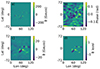 |
Fig. 1. Filtering steps for near-side magnetograms. Data are from December 10, 2015. a) HMI magnetogram. b) Phase-shift map of the same region on the far-side half one rotation earlier (13.5 days). c) Magnetogram after resizing and applying Gaussian smoothing where regions that emerged on the near side have been removed. d) Final magnetograms with nine magnetic field levels. |
We masked every active region that emerged on the near side and paired the magnetogram sequences with sequences of 11 far-side phase-shift maps from half a solar rotation before (13.5 days). These pairs of magnetogram-seismic maps probe the same region of the solar surface although they are not cotemporal. The masking process of the near-side emerged regions was the same as described in Felipe & Asensio Ramos (2019). Then, each masked magnetogram and those that did not need masking went through a Gaussian smoothing with a standard deviation of 3 degrees. Finally, each value of the magnetogram was binned into nine levels, each level representing a range in magnetic fields. The bin boundaries are listed in Table 1. These bins were chosen to be equispaced in the percentile of the magnetic field value among all the pixels of the used magnetograms, first by creating 11 equispaced levels, and then by joining the two levels at each side of the central one. Those with a magnetic field strength below ∼10 G were considered inactive points. The three most extreme limit values for the levels were manually modified to percentiles 0.2, 2.5, and 12 on the negative side and to percentiles 88, 97.5, and 99.8 on the positive side. This was made after some trial and error procedures to ensure that the representation of high magnetic field values was sufficient. The wider range of the levels with a higher magnetic field modulus was selected as a compromise between network performance and magnetic field resolution. The quantization listed in Table 1 was chosen after evaluating the performance of several different criteria using the volumetric Dice metric (see Sect. 3). We considered other quantizations, such as considering equispaced bins in the magnetic field percentile (without changing the extreme levels) and equispaced bins in the magnetic field, but they were discarded in favor of those in Table 1. The whole process we applied to the magnetograms is illustrated in Fig. 1.
Limit magnetic field values for each range represented by integer numbers between 0 and 8 in the magnetograms we used as elements of the training output sequences for FarNet-II.
2.2.2. Training
Magnetograms from May 2010 to April 2019 were used to compute the training targets, which resulted in 6071 sequences of 11 consecutive binned magnetograms taken with a cadence of 12 hours. Augmenting was applied during the training to double the available data. To do this, we flipped the images over the latitude axis and changed the polarity of the magnetograms, so that the magnetograms remained consistent with Hale’s law. We used a cross-validation scheme for the training and the evaluation, training through 33 runs and keeping 160 different consecutive sequences out of the training set for each one of them. These sequences were not superposed with training data and were used for the evaluation.
During neural network training, a loss function was computed at each iteration to quantify the discrepancy between the network-predicted outputs and the expected values for a given input. The gradients of the loss function with respect to the network weights were then calculated, indicating how the weights should be adjusted to optimize the network performance. Ideally, the loss function value should be minimized by the end of the training process, reflecting the improved accuracy of the model. The loss function minimized during this training was a variant of the hybrid focal loss proposed by Yeung et al. (2021). This loss is a mixture of the focal loss (Lin et al. 2020) and the Tversky focal loss (Abraham & Khan 2019). It is especially useful for unbalanced datasets such as ours. The representation of different classes in the training is uneven although the binning of the magnetograms is based on percentiles, because exceptions were imposed. Each FarNet-II output for a phase-shift map input was a set of nine matrices, each one containing predictions for one bin of the magnetic field (see Table 1). We applied a softmax to the output of FarNet-II to ensure that the values of the magnetic field range in every pixel can be regarded as probabilities.
The focal loss is based on the cross-entropy loss, which is ultimately based on information theory concepts. It measures the difference between two probability distributions, with a lower loss being associated with more similar probability distributions. Cross-entropy, for the binary case (one class to be predicted), can be written as
 (1)
(1)
where y and p are restricted to values in the [0,1] range and represent the ground-truth label and the predicted value, respectively. Binary cross-entropy can also be written as
 (2)
(2)
It can be simplified by defining
 (3)
(3)
so that we can write
 (4)
(4)
For the binary case, the focal loss is defined as
 (5)
(5)
where α and γ are tunable parameters. For the multiclass case, this can be generalized as
 (6)
(6)
with the subscript c indicating one specific magnetic value channel (magnetic levels for FarNet-II), and C being the total number of magnetic value channels on the outputs.
The Tversky loss is a variation of the Dice loss, which measures the boolean superposition between two tensors, with a lower loss being the result of a higher superposition. The Tversky loss can be written as
 (7)
(7)
where TI is the Tversky index, defined as
 (8)
(8)
In this expression, p0i is the probability that the pixel i belongs to the foreground (classified as the target) and p1i is the probability that the same pixel belongs to the background (classified as different from the target). The parameter N represents the number of pixels. The parameter g0i is one when the pixel belongs to the foreground and zero otherwise, and g1i takes the value of |1 − g0i|. A hyperparameter that balances the relative importance of false negatives and false positives is expressed with δ in the equation.
The focal Tversky loss takes the form
 (9)
(9)
where γt is a hyperparameter, and it can be generalized to the multiclass case with the equation
 (10)
(10)
The hybrid loss that we used in this work is defined as the following convex combination:
 (11)
(11)
using the hyperparameter λ, suggested as a modification by Yeung et al. (2022). The hybrid loss was applied over each element of the output sequence (11 predictions), and the results were then averaged over the whole sequence. The parameter β was introduced to ensure that both losses contribute to the final loss, given the large differences in their values. A value of β = 10 was used.
We performed a hyperparameter tuning for the values δ and λ. We only tuned these two hyperparameters because they were considered to be the most relevant. The remaining hyperparameters were set to the recommended values (γt = 4/3, γ = 2, α = 1) given for semantic segmentation tasks by Lin et al. (2020) and Abraham & Khan (2019). The tuning was made using a training set of which three portions of 160 sequences each were left out for validation. Each left-out portion was taken in a different period of the solar cycle, ensuring that we had a good sampling of the variable magnetic activity of the Sun. Then, we evaluated the results for each validation set using a newly defined metric that we call “volumetric Dice” (see Sect. 3). The tuning of the hyperparameters of the hybrid loss obtained using this evaluation metric yielded the values δ = 0.8 and λ = 0.2.
Both the model and the training script were written using the open-source PyTorch library (Paszke & Gross 2019). The loss function was reimplemented in PyTorch from its original implementation of Yeung et al. (2022)3. The optimization was made using the Adam optimizer (Kingma & Ba 2017), with a learning rate of 3 × 10⁻⁴ and a batch size of 2. A total of five epochs was sufficient for the validation loss to converge.
2.2.3. Postprocesing
As explained in the previous section, each FarNet-II output for a phase-shift map input is a set of nine matrices, each one containing predictions for one level of the magnetic field of the levels listed in Table 1. This means that postprocessing is needed to construct magnetogram images as those used as targets of the training. This was carried out through the application of a softmax function over the channel dimension (to transform the results into probabilities) and the determination of the channel with the highest probability for each pixel of the bidimensional map. After the highest probability channel was determined, the pixel of the 2D magnetogram was assigned the corresponding class.
3. Evaluation method
To compute the similarity between the magnetogram masks and the outputs of the network on the validation data of the cross-validation study, we used the volumetric Dice. This is a newly defined metric. It measures the overlap of magnetograms and outputs by using for each one of them a volumetric representation computed through the next steps. First, we created a cube with zeros whose dimensions are latitude, longitude, and channel. The channel dimension had a size 9, where each channel represents the magnetic range assigned to each pixel. Second, for each pixel, we set a value of one on the predicted channel (or on the target channel for the targets) and all channels with lower magnetic fields with the same sign. Finally, the Dice coefficient between the predicted and target data cubes was computed. A higher Dice means a higher similarity between them, with a volumetric Dice of one when the coincidence is absolute. This value of one is hard to achieve given the resolution of the phase-shift maps that are input to the network, which cannot lead to perfect predictions, and the inaccuracies introduced when extrapolating the magnetic field from the phase-shift, which is not a perfect proxy, but is the best that we have for the far side when cotemporal observations are lacking. The Dice coefficient is computed according to its standard definition,
 (12)
(12)
where i(lat, lon, ch) and o(lat, lon, ch) are the values of the output and target data cubes for each pixel (latitude, longitude, and channel coordinates), while ϵ is a small quantity (0.001 for this work) that prevents the Dice coefficient from being undefined.
This metric has the advantage of capturing the partial coincidence of active region detections while only taking into account results with the correct polarity. This approach offers advantages over the regular Dice coefficient because in the case of the latter, a difference of one channel between the prediction and the target would produce zero overlap. The volumetric Dice coefficient
tolerates small differences in the prediction and better suits our objectives with FarNet-II. An example is shown in Fig. 2, where the output magnetogram of FarNet-II is shown for January 30, 2014. This date was not part of the training set. Its volumetric representation is shown in panel c. Panels b and d show the target magnetogram and its volumetric representation, respectively.
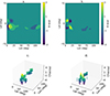 |
Fig. 2. Example of volumetric processing for the output of FarNet-II to evaluate their posterior similarity. Panel a shows the output magnetogram of FarNet-II for January 30, 2014. Panel b shows the corresponding target magnetogram. Panels c and d show the volumetric representations of the output and the target magnetograms, respectively. |
4. Results
4.1. Qualitative comparisons
Figures 3 and 4 show the FarNet-II activity predictions for two different sequences of seismic maps. For visual clarity, only 5 elements with a temporal cadence of 24 hours are displayed for each of them, instead of the full 11-element prediction. The dates of these inferences were selected to illustrate the Farnet-II performance under different activity conditions. Figure 3 shows predictions for a sequence of days near the activity maximum of cycle 24, and Fig. 4 represents predictions for a low-activity period.
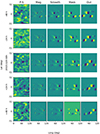 |
Fig. 3. Representation of FarNet-II predictions for activity in a sequence centered on November 20, 2013. Only 5 of the 11 elements of the sequence are shown, with a cadence of 24 hours. The first column shows the phase-shift maps we used as inputs of the network. The second column shows the related near-side magnetogram, 13.5 days later. The third column shows the smoothed magnetograms. The fourth column shows the mask and targets of the training (binned magnetograms), and the last column shows the FarNet-II outputs. |
A visual comparison of the network output (last column) and the targets of the training (fourth column) reveals a fairly good agreement, especially for large active regions. The network correctly extrapolates Hale’s law from the training data. Since FarNet-II was trained with data from solar cycle 24, the application of the network to data from odd solar cycles requires a reversion of the output polarity. Moreover, the outputs capture the tilt of the active regions. Figure 4 shows that the predicted leading spot is closer to the equator, in agreement with the target and in accordance with Joy’s law. The bottom rows in Fig. 3 show that the network cannot capture the complexity of tangled active regions as easily. In these cases, the output instead exhibits a larger bipolar region.
4.2. Quantitative comparisons
Figure 5 shows the variation in the volumetric Dice for each training in the cross-validation study, measured on the validation split, without overlap with the training data. The volumetric Dice generally exhibits values between 0.2 and 0.3, except for the last sets, which have striking high volumetric Dice values. These sets correspond to time periods with low solar activity, where maps without activity in the output and target are common. In the case of these maps, the Dice takes values closer to one, and therefore, sets with low activity tend to exhibit a higher average volumetric Dice. The mean Dice of all the validation sets is 0.249. The higher Dice for periods with significant solar activity is 0.394. This is found, for the training that left out the validation set 14, centered on December 6, 2013. In contrast, the lowest Dice of 0.035 is obtained for set 28, centered on July 27, 2017.
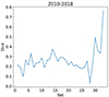 |
Fig. 5. Mean volumetric Dice as a function of the validation set for the 33 sets used in the cross-validation scheme. It is averaged for every element of the sequence for all the sequences in each set. |
Generally, the overlap between the target and the predictions of FarNet-II is high, and the predictions are mostly accurate. Figure 6 illustrates a comparison for a sample of typical values of the volumetric Dice coefficient from poor (volumetric Dice of 0.13) to excellent predictions (volumetric Dice of 0.56). Figure 6 visually approximates the meaning of the volumetric Dice by illustrating the relation between its values and the quality of the prediction. In its second row, we show an example of volumetric Dice 0.25, which is approximately the mean value achieved with FarNet-II.
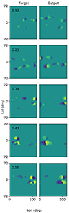 |
Fig. 6. Examples of pairs that were target-output for magnetograms predicted by FarNet-II. Each target is paired with its output in the same row. The number on the upper left side of the targets is the achieved volumetric Dices for each case. |
Figure 7 shows the correlation between the inferred and actual magnetic fields from the target data. It exhibits a clear linear correlation, which proves that the network accurately detects the magnetic field strength and polarity for most predictions. The magnetic field is slightly underestimated in general, with a preference for predictions closer to the central bins. Additionally, we find that a certain number of active regions remains undetected even for large target magnetic fields.
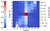 |
Fig. 7. Fraction of pixels from each magnetic level of the targets assigned to each magnetic level of the outputs. The values are normalized to the total number of pixels of this subset assigned to each level of the targets. The right y-axis shows the magnetic field intervals associated with each level. The exact limits for the magnetic field range of each level are shown in Table 1. |
5. Comparison with Solar Orbiter
Solar Orbiter (Müller et al. 2020) is a scientific observatory that was launched in February 2020 to observe the Sun at a closer distance than ever before and from vantage points that allow the observation of solar regions that are inaccessible from the Earth, such as the solar poles or the far side. One of the instruments on board Solar Orbiter is the Polarimetric and Helioseismic Imager (PHI, Solanki et al. 2020), which provides magnetograms of the surface of the Sun, among other types of data. Routine science operations started in November 2021. Between May and October 2022, a large data set with far-side coverage was acquired. This dataset is available at the Solar Orbiter Archive4. We computed the FarNet-II far-side predictions for some of the dates that are included in this dataset. The results were compared with far-side magnetograms that were directly acquired by Solar Orbiter at the same time as our predictions.
As a first step, the network was retrained with all the available data from all the training sets. The cross-validation setup is no longer necessary because we applied Farnet II to data beyond the period employed for the training. Because the network was trained in an even cycle and was applied in this section to data from an uneven cycle, the polarity of the outputs was flipped. This ensured that the predictions follow Hale’s law.
We computed outputs for dates between May 1, 2022, and September 20, 2022, for days 1, 5, 10, 15, 20, and 25 of each month, or for the closest available date. Then, we compared the outputs to the cotemporal Solar Orbiter magnetogram masks of the far side. They were computed in the same fashion as those of HMI that were employed for the training (see Sect. 2.2.1). We also compared the outputs to HMI data from 13.5 days later in the form of magnetogram masks such as those used in training. The metric used for this comparison is the same as we used for the general evaluation of the network in the previous sections, the volumetric Dice. The results of this comparison for each date are shown in Fig. 8, where the volumetric Dices from HMI and Solar Orbiter are compared. The X-axis represents HMI data, and the Y-axis represents Solar Orbiter data. Most points fall close to the diagonal, showing that the accuracy of the predictions is very similar for HMI and Solar Orbiter data. The average volumetric Dices for Solar Orbiter and HMI data were 0.32 and 0.25, respectively. Examples of representative cases and their respective volumetric Dices are shown in Fig. 9. This figure shows that for a diverse range of volumetric Dices, the network returns predictions that are similar to the magnetic masks, especially for Solar Orbiter, because its data are cotemporal with the predictions. The only case in which the predictions are qualitatively and quantitatively worse is the case with very low activity (top row). For this case, FarNet-II is not able to predict any activity.
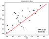 |
Fig. 8. Volumetric Dices for HMI (X-axis) and Solar Orbiter (SO in the figure) (Y-axis) for the study of Section 5. The HMI Dices are calculated for outputs from 13.5 days later than the Solar Orbiter data when activity has rotated to the near-side hemisphere, from which the HMI data are taken. The points represent data from May 1 to September 20, 2022, with a cadence of 5 days. The diagonal is shown in red for reference. The average volumetric Dices for HMI and Solar Orbiter are shown in the lower right corner. |
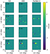 |
Fig. 9. Comparisons between the FarNet-II outputs (last column), HMI magnetogram masks from 13.5 days later (second column), and Solar Orbiter (SO in the figure) far-side magnetogram masks taken at the time of the network outputs (first column). The number in the upper left corner indicates the volumetric Dice calculated for each specific mask and the FarNet-II output for the corresponding date. |
6. Discussion and conclusions
We developed a machine-learning algorithm to predict the line-of-sight magnetic field, including its polarity, of far-side active regions. The large data set we used for the training provided enough statistics to the network to infer Hale’s and Joy’s laws and to associate the seismic signal of active regions with magnetograms that followed these two well-known empirical laws. Our results (see Sect. 4) show that the network can correctly predict the level of activity and the polarity for most of the cases. The network performance was evaluated in data sets that were similar to those employed for the training (using near-side magnetograms acquired half a rotation later than the far-side seismic maps), but also by comparing the network predictions with cotemporal magnetograms observed with Solar Orbiter.
One of the limitations of the far-side magnetogram predictions is the low spatial resolution of the far-side seismic data. The resolution of the helioseismic maps depends on the incidence angle of the waves employed for the computation, which is close to vertical for far-side helioseismology. For the wave configuration employed for the seismic data we used, the spatial resolution is about 10 degrees of arc over the solar surface (Lindsey & Braun 2017). Following the same strategy as for FarNet (Felipe & Asensio Ramos 2019) and FarNet-II (Broock et al. 2022), we performed a Gaussian smoothing of the target magnetograms. The low resolution of the network output does not compromise its application to space-weather forecasting because models of the corona and solar wind (e.g., CORHEL, Mikić et al. 1999) generally employ a smoothed photospheric radial magnetic field as a boundary condition. The models are sufficient to correctly predict the size and location of coronal holes, which are the main precursors of variation in the solar wind speed.
Another limitation is the training with magnetograms that are not cotemporal to the seismic maps. Although the method neglects the evolution of the active region magnetic configuration between the two measurements, the positive comparison of FarNet-II predictions with cotemporal magnetograms observed with Solar Orbiter supports the validity of the approach.
Our study is a new contribution to the renewed interest in far-side helioseismology. In recent years, several works have aimed to improve the predictions using neural networks (Felipe & Asensio Ramos 2019; Broock et al. 2021, 2022; Chen et al. 2022) and novel implementations of time-distance (Zhao et al. 2019) and helioseismic holography (Yang et al. 2023a,b) methods. These efforts and future works will lead to the systematic incorporation of far-side helioseismic inferences in models for space-weather forecasts.
Acknowledgments
We thank C. Lindsey, from North-West Research Associates (NWRA), for allowing us to use the routines his team built for the latitude-longitude projections of the magnetograms. We also thank C. Cid, from Universidad de Alcalá de Henares (UAH), for her invaluable ideas for future projects using FarNet-II. Financial support from grants PGC2018-097611-A-I00, PID2021-127487NB-I00, and PID2022-136563NB-I00, funded by MCIN/AEI/ 10.13039/501100011033 and by “ERDF A way of making Europe”, and grant PROID2020010059 funded by Consejería de Economía, Conocimiento y Empleo del Gobierno de Canarias and the European Regional Development Fund (ERDF) is gratefully acknowledged. TF acknowledges grant RYC2020-030307-I funded by MCIN/AEI/ 10.13039/501100011033 and by “ESF Investing in your future”. The open data policy of Solar Orbiter data is also appreciated. We acknowledge the community effort devoted to the development of the following open-source packages that were used in this work: numpy (numpy.org, Harris et al. 2020), matplotlib (matplotlib.org, Hunter 2007), PyTorch (pytorch.org, Paszke & Gross 2019), and SunPy (sunpy.org, The SunPy Community 2020), einops (Rogozhnikov 2022), and h5py (Koziol & Robinson 2018).
References
- Abraham, N., & Khan, N. M. 2019, 2019 IEEE 16th International Symposium on Biomedical Imaging (ISBI 2019), 683 [CrossRef] [Google Scholar]
- Arge, C. N., Henney, C. J., Hernandez, I. G., et al. 2013, Solar Wind 13, 1539, 11 [Google Scholar]
- Bahdanau, D., Cho, K., & Bengio, Y. 2014, ArXiv e-prints [arXiv:1409.0473] [Google Scholar]
- Boulila, W., Ghandorh, H., Khan, M. A., Ahmed, F., & Ahmad, J. 2021, ArXiv e-prints [arXiv:2103.01695] [Google Scholar]
- Braun, D., & Lindsey, C. 2000, Sol. Phys., 192, 307 [NASA ADS] [CrossRef] [Google Scholar]
- Braun, D. C., Duvall, T. L., Jr, & Labonte, B. J. 1987, ApJ, 319, L27 [NASA ADS] [CrossRef] [Google Scholar]
- Braun, D., Lindsey, C., Fan, Y., & Jefferies, S. 1992, APJ, 392, 739 [CrossRef] [Google Scholar]
- Broock, E. G., Felipe, T., & Asensio Ramos, A. 2021, A&A, 652, A9 [Google Scholar]
- Broock, E. G., Asensio Ramos, A., & Felipe, T. 2022, A&A, 667, A10 [Google Scholar]
- Chen, R., Zhao, J., Webber, S. H., et al. 2022, APJ, 941, 197 [CrossRef] [Google Scholar]
- Christensen-Dalsgaard, J. 2002, Rev. Mod. Phys., 74, 1073 [Google Scholar]
- Duvall, T. L., Jr, & Kosovichev, A. G. 2001, IAU Symp., 203, 159 [NASA ADS] [Google Scholar]
- Duvall, T. L., Jr, Jefferies, S. M., Harvey, J. W., & Pomerantz, M. A. 1993, Nature, 362, 430 [Google Scholar]
- Felipe, T., & Asensio Ramos, A. 2019, A&A, 632, A82 [NASA ADS] [CrossRef] [EDP Sciences] [Google Scholar]
- Felipe, T., Braun, D. C., & Birch, A. C. 2017, A&A, 604, A126 [NASA ADS] [CrossRef] [EDP Sciences] [Google Scholar]
- Fillioux, L. 2020, attentionblock.py, https://gist.github.com/leofillioux, accessed: 2021-11-30 [Google Scholar]
- Fontenla, J. M., Quémerais, E., González Hernández, I., Lindsey, C., & Haberreiter, M. 2009, ASR, 44, 457 [Google Scholar]
- Fu, J., Liu, J., Tian, H., et al. 2019, ArXiv e-prints [arXiv:1809.02983] [Google Scholar]
- González Hernández, I., Hill, F., & Lindsey, C. 2007, ApJ, 669, 1382 [CrossRef] [Google Scholar]
- Goodfellow, I., Bengio, Y., & Courville, A. 2016, Deep Learning (MIT Press) [Google Scholar]
- Hanson, A., Pnvr, K., Krishnagopal, S., & Davis, L. 2019, Bidirectional Convolutional LSTM for the Detection of Violence in Videos: Subvolume B, 280 [Google Scholar]
- Harris, C. R., Millman, K. J., van der Walt, S. J., et al. 2020, Nature, 585, 357 [NASA ADS] [CrossRef] [Google Scholar]
- Harvey, J. W., Hill, F., Hubbard, R. P., et al. 1996, Science, 272, 1284 [Google Scholar]
- Hill, F. 1988, ApJ, 333, 996 [Google Scholar]
- Hochreiter, S., & Schmidhuber, J. 1997, Neural Comput., 9, 1735 [CrossRef] [Google Scholar]
- Hu, J., Shen, L., Albanie, S., Sun, G., & Wu, E. 2019, ArXiv e-prints [arXiv:1709.01507] [Google Scholar]
- Hunter, J. D. 2007, CiSE, 9, 90 [Google Scholar]
- Ilonidis, S., Zhao, J., & Hartlep, T. 2009, Sol. Phys., 258, 181 [NASA ADS] [CrossRef] [Google Scholar]
- Ioffe, S., & Szegedy, C. 2015, in Proceedings of the 32nd International Conference on Machine Learning (ICML-15) (JMLR Workshop and Conference Proceedings) [Google Scholar]
- Kaiser, M. 2004, ASR, 36, 1483 [Google Scholar]
- Kim, T., Park, E., Lee, H., et al. 2019, Nat. Astron., 3, 397 [Google Scholar]
- Kingma, D. P., & Ba, J. 2017, ArXiv e-prints [arXiv:1412.6980] [Google Scholar]
- Koziol, Q., & Robinson, D. 2018, HDF5, [Computer Software] https://doi.org/10.11578/dc.20180330.1 [Google Scholar]
- Lemen, J. R., Title, A. M., Akin, D. J., et al. 2012, Sol. Phys., 275, 17 [Google Scholar]
- Liewer, P. C., González Hernández, I., Hall, J. R., Lindsey, C., & Lin, X. 2014, Sol. Phys., 289, 3617 [NASA ADS] [CrossRef] [Google Scholar]
- Liewer, P. C., Qiu, J., & Lindsey, C. 2017, Sol. Phys., 292, 146 [NASA ADS] [CrossRef] [Google Scholar]
- Lin, T. -Y., Goyal, P., Girshick, R., He, K., & Dollár, P. 2020, Focal Loss for Dense Object Detection, in {IEEE Transactions on Pattern Analysis and Machine Intelligence}, 42, 318, https://doi.org/10.1109/TPAMI.2018.2858826 [CrossRef] [Google Scholar]
- Lindsey, C., & Braun, D. C. 1990, Sol. Phys., 126, 101 [NASA ADS] [CrossRef] [Google Scholar]
- Lindsey, C., & Braun, D. C. 2000a, Science, 287, 1799 [Google Scholar]
- Lindsey, C., & Braun, D. C. 2000b, Sol. Phys., 192, 261 [Google Scholar]
- Lindsey, C., & Braun, D. 2017, Space Weather, 15, 761 [NASA ADS] [CrossRef] [Google Scholar]
- Lindsey, C., Cally, P. S., & Rempel, M. 2010, ApJ, 719, 1144 [NASA ADS] [CrossRef] [Google Scholar]
- MacDonald, G. A., Henney, C. J., Díaz Alfaro, M., et al. 2015, ApJ, 807, 21 [NASA ADS] [CrossRef] [Google Scholar]
- Mikić, Z., Linker, J. A., Schnack, D. D., Lionello, R., & Tarditi, A. 1999, Phys. Plasmas, 6, 2217 [Google Scholar]
- Müller, D., St. Cyr, O. C., Zouganelis, I., et al. 2020, A&A, 642, A1 [Google Scholar]
- Nair, V., Hinton, G. E., et al. 2010, in Proceedings of the 27th International Conference on Machine Learning (ICML-10), June 21–24, 2010, Haifa, Israel, 807 [Google Scholar]
- Oktay, O., Schlemper, J., Folgoc, L. L., et al. 2018, ArXiv e-prints [arXiv:1804.03999] [Google Scholar]
- Paszke, A., & Gross, S. 2019, Adv Neural Inf Process Syst 32 (Curran Associates, Inc.) [Google Scholar]
- Rogozhnikov, A. 2022, ICLR, https://openreview.net/forum?id=oapKSVM2bcj [Google Scholar]
- Ronneberger, O., Fischer, P., & Brox, T. 2015, ArXiv e-prints [arXiv:1505.04597] [Google Scholar]
- Rumelhart, D. E., Hinton, G. E., & Williams, R. J. 1986, Parallel Distributed Processing: Explorations in the Microstructure of Cognition, Volume 1: Foundations (MIT Press) [CrossRef] [Google Scholar]
- Scherrer, P. H., Bogart, R. S., Bush, R. I., et al. 1995, Sol. Phys., 162, 129 [Google Scholar]
- Schou, J., Scherrer, P. H., Bush, R. I., et al. 2012, Sol. Phys., 275, 229 [Google Scholar]
- Schunker, H., Gizon, L., Cameron, R. H., & Birch, A. C. 2013, A&A, 558, A130 [NASA ADS] [CrossRef] [EDP Sciences] [Google Scholar]
- Shi, X., Chen, Z., Wang, H., et al. 2015, ArXiv e-prints [arXiv:1506.04214] [Google Scholar]
- Solanki, S. K., del Toro Iniesta, J. C., Woch, J., et al. 2020, A&A, 642, A11 [NASA ADS] [CrossRef] [EDP Sciences] [Google Scholar]
- Srivastava, N., Hinton, G., Krizhevsky, A., Sutskever, I., & Salakhutdinov, R. 2014, JMLR, 15, 1929 [Google Scholar]
- The SunPy Community (Barnes, W. T., et al.) 2020, APJ, 890, 68 [CrossRef] [Google Scholar]
- Vaswani, A., Shazeer, N., Parmar, N., et al. 2017, ArXiv e-prints [arXiv:1706.03762] [Google Scholar]
- Yang, D., Gizon, L., & Barucq, H. 2023a, A&A, 669, A89 [NASA ADS] [CrossRef] [EDP Sciences] [Google Scholar]
- Yang, D., Gizon, L., Barucq, H., et al. 2023b, A&A, 674, A183 [NASA ADS] [CrossRef] [EDP Sciences] [Google Scholar]
- Yeung, M., Sala, E., Schönlieb, C.-B., & Rundo, L. 2021, Comput. Biol. Med., 137, 104815 [CrossRef] [Google Scholar]
- Yeung, M., Sala, E., Schönlieb, C.-B., & Rundo, L. 2022, CMIG, 95, 102026 [Google Scholar]
- Zeiler, M., Krishnan, D., Taylor, G., & Fergus, R. 2010, 2010 IEEE Computer Society Conference on Computer Vision and Pattern Recognition, CVPR 2010, 2528 [Google Scholar]
- Zhao, J. 2007, ApJ, 664, L139 [NASA ADS] [CrossRef] [Google Scholar]
- Zhao, J., Hing, D., Chen, R., & Hess Webber, S. 2019, ApJ, 887, 216 [NASA ADS] [CrossRef] [Google Scholar]
All Tables
Limit magnetic field values for each range represented by integer numbers between 0 and 8 in the magnetograms we used as elements of the training output sequences for FarNet-II.
All Figures
|
Fig. 1. Filtering steps for near-side magnetograms. Data are from December 10, 2015. a) HMI magnetogram. b) Phase-shift map of the same region on the far-side half one rotation earlier (13.5 days). c) Magnetogram after resizing and applying Gaussian smoothing where regions that emerged on the near side have been removed. d) Final magnetograms with nine magnetic field levels. |
| In the text | |
|
Fig. 2. Example of volumetric processing for the output of FarNet-II to evaluate their posterior similarity. Panel a shows the output magnetogram of FarNet-II for January 30, 2014. Panel b shows the corresponding target magnetogram. Panels c and d show the volumetric representations of the output and the target magnetograms, respectively. |
| In the text | |
|
Fig. 3. Representation of FarNet-II predictions for activity in a sequence centered on November 20, 2013. Only 5 of the 11 elements of the sequence are shown, with a cadence of 24 hours. The first column shows the phase-shift maps we used as inputs of the network. The second column shows the related near-side magnetogram, 13.5 days later. The third column shows the smoothed magnetograms. The fourth column shows the mask and targets of the training (binned magnetograms), and the last column shows the FarNet-II outputs. |
| In the text | |
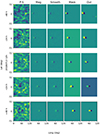 |
Fig. 4. Same as Fig. 3, but for the sequence centered on July 13, 2018. |
| In the text | |
|
Fig. 5. Mean volumetric Dice as a function of the validation set for the 33 sets used in the cross-validation scheme. It is averaged for every element of the sequence for all the sequences in each set. |
| In the text | |
|
Fig. 6. Examples of pairs that were target-output for magnetograms predicted by FarNet-II. Each target is paired with its output in the same row. The number on the upper left side of the targets is the achieved volumetric Dices for each case. |
| In the text | |
|
Fig. 7. Fraction of pixels from each magnetic level of the targets assigned to each magnetic level of the outputs. The values are normalized to the total number of pixels of this subset assigned to each level of the targets. The right y-axis shows the magnetic field intervals associated with each level. The exact limits for the magnetic field range of each level are shown in Table 1. |
| In the text | |
|
Fig. 8. Volumetric Dices for HMI (X-axis) and Solar Orbiter (SO in the figure) (Y-axis) for the study of Section 5. The HMI Dices are calculated for outputs from 13.5 days later than the Solar Orbiter data when activity has rotated to the near-side hemisphere, from which the HMI data are taken. The points represent data from May 1 to September 20, 2022, with a cadence of 5 days. The diagonal is shown in red for reference. The average volumetric Dices for HMI and Solar Orbiter are shown in the lower right corner. |
| In the text | |
|
Fig. 9. Comparisons between the FarNet-II outputs (last column), HMI magnetogram masks from 13.5 days later (second column), and Solar Orbiter (SO in the figure) far-side magnetogram masks taken at the time of the network outputs (first column). The number in the upper left corner indicates the volumetric Dice calculated for each specific mask and the FarNet-II output for the corresponding date. |
| In the text | |
Current usage metrics show cumulative count of Article Views (full-text article views including HTML views, PDF and ePub downloads, according to the available data) and Abstracts Views on Vision4Press platform.
Data correspond to usage on the plateform after 2015. The current usage metrics is available 48-96 hours after online publication and is updated daily on week days.
Initial download of the metrics may take a while.