| Issue |
A&A
Volume 669, January 2023
|
|
|---|---|---|
| Article Number | A39 | |
| Number of page(s) | 13 | |
| Section | The Sun and the Heliosphere | |
| DOI | https://doi.org/10.1051/0004-6361/202244663 | |
| Published online | 03 January 2023 | |
Stellar signal components seen in HARPS and HARPS-N solar radial velocities⋆
1
Observatoire Astronomique de l’Université de Genève, Chemin Pegasi 51, 1290 Versoix, Switzerland
e-mail: This email address is being protected from spambots. You need JavaScript enabled to view it.
2
Instituto de Astrofísica e Ciências do Espaço, Universidade do Porto, CAUP, Rua das Estrelas, 4150-762 Porto, Portugal
3
European Southern Observatory, Avenida Alonso de Cordova 3107, Santiago de Chile, Chile
4
Departamento de Física e Astronomia, Faculdade de Ciências, Universidade do Porto, Rua do Campo Alegre, 4169-007 Porto, Portugal
Received:
2
August
2022
Accepted:
7
November
2022
Abstract
Context. Radial velocity (RV) measurements induced by the presence of planets around late-type stars are contaminated by stellar signals that are on the order of a few meters per second in amplitude, even for the quietest stars. Those signals are induced by acoustic oscillations, convective granulation patterns, active regions corotating with the stellar surface, and magnetic activity cycles.
Aims. This study investigates the properties of all coherent stellar signals seen on the Sun on timescales up to its sidereal rotational period. By combining HARPS and HARPS-N solar data spanning several years, we are able to clearly resolve signals on timescales from minutes to several months.
Methods. We used a Markov chain Monte Carlo (MCMC) mixture model to determine the quality of the solar data based on the expected airmass–magnitude extinction law. We then fit the velocity power spectrum of the cleaned and heliocentric RVs with all known variability sources, to recreate the RV contribution of each component.
Results. After rejecting variations caused by poor weather conditions, we were able to improve the average intra-day root mean square (rms) value by a factor of ∼1.8. On sub-rotational timescales, we were able to fully recreate the observed rms of the RV variations. In order to also include rotational components and their strong alias peaks introduced by nightly sampling gaps, the alias powers were accounted for by being redistributed to the central frequencies of the rotational harmonics.
Conclusions. In order to enable a better understanding and mitigation of stellar activity sources, their respective impact on the total RV must be well measured and characterized. We were able to recreate RV components up to rotational timescales, which can be further used to analyze the impact of each individual source of stellar signals on the detectability of exoplanets orbiting very quiet solar-type stars and test the observational strategies of RV surveys.
Key words: stars: activity / stars: individual: Sun / techniques: radial velocities
The radial velocities are only available at the CDS via anonymous ftp to cdsarc.cds.unistra.fr (130.79.128.5) or via https://cdsarc.cds.unistra.fr/viz-bin/cat/J/A+A/669/A39
© The Authors 2023
 Open Access article, published by EDP Sciences, under the terms of the Creative Commons Attribution License (https://creativecommons.org/licenses/by/4.0), which permits unrestricted use, distribution, and reproduction in any medium, provided the original work is properly cited.
This article is published in open access under the Subscribe-to-Open model. This email address is being protected from spambots. You need JavaScript enabled to view it. to support open access publication.
1. Introduction
The external convective layers of late-type main-sequence stars give rise to several types of stellar signals seen in radial velocity (RV) measurements, with timescales ranging from minutes to years (see e.g., Kjeldsen & Bedding 1995; Saar & Donahue 1997; Schrijver & Zwaan 2000; Lindegren & Dravins 2003; Christensen-Dalsgaard 2004; Kjeldsen et al. 2005; Meunier et al. 2010, 2015; Dumusque et al. 2011a,b; Dumusque 2016). The field of astroseismology, which studies stellar oscillations induced by acoustic waves propagating in the convective layer of late-type stars, has been established for a long time (Goldreich & Keeley 1977), and is useful in the mass and age determination of main-sequence stars, and the mass and radius determination of giant stars. More recently, the importance of understanding stellar signals has been extended to the field of exoplanets. Since the first discovery of an extra-solar planet orbiting a solar-like star by Mayor & Queloz (1995), more than 7800 candidates have been detected, and the planetary status has been confirmed for 5200 of them1. A significant fraction of those planets have been either detected or confirmed using the RV technique, which allows the presence of planets to be confirmed by measuring the Doppler shift they induced on their host stars’ spectra.
For state-of-the-art spectrographs, which are able to reach sub-meter-per-second RV precision, stellar activity is the main limitation to the detection of Earth-like planets, but also more massive planets at larger separation, as it induces RV variations that are one to two orders of magnitude larger than such planets. It is therefore crucial to better understand the different types of stellar signals, and to find mitigation techniques to correct RVs from them. Our understanding of the different types of stellar signals for solar-like stars vastly improved thanks to the HARPS spectrograph (Mayor et al. 2003) at the ESO 3.6 m Telescope, which was the first instrument to reach the meter-per-second precision level, and therefore it was able to measure all the different contributions of stellar signals, from the short-term acoustic oscillations, to the long-term magnetic cycles.
On the timescale of minutes, the excitation of acoustic oscillations, known as pressure waves (or p-modes), expands and contracts the stellar surface with different types of modes (e.g., Kjeldsen & Bedding 1995; Christensen-Dalsgaard 2004; Kjeldsen et al. 2005). These oscillations have been shown to be easily averaged out by selecting an observing strategy with a sufficiently long (about 5 minutes for the Sun) exposure time (e.g., Dumusque et al. 2011b; Chaplin et al. 2019).
On timescales from dozens of minutes to a few days, granulation phenomena on various spatial scales (granulation, supergranulation, e.g., Del Moro 2004; Del Moro et al. 2004), driven by the convective motion in the external envelopes of solar-like stars, induce an RV signal with an amplitude of a few meters per second (Dumusque et al. 2011b; Cegla et al. 2013; Meunier et al. 2015). Those signals can be averaged out in RV measurements by observing a star several times per night (Dumusque et al. 2011b), in order to sample different phases of the granulation phenomena signal. However, such a strategy cannot fully mitigate the supergranulation signal due to its timescale that is longer than a day, as demonstrated in Meunier et al. (2015). There is, however, hope that granulation phenomenon signals can be mitigated by precisely measuring spectral line shape variations (Cegla et al. 2019).
Radial velocity modulations of a few meters per second on the stellar rotational timescale originate from active regions corotating with the stellar surface (e.g., Saar & Donahue 1997; Meunier et al. 2010; Dumusque et al. 2011a, 2014; Herrero et al. 2016). These regions appear in conjunction with strong magnetic surface fields. They manifest themselves as either spots, which are regions of strong magnetic field and low temperature contrast compared to the quiet star, and thus appear dark, or as faculae, which are regions of weaker magnetic field and of slightly higher temperature than the quiet star, usually surrounding spots but also found in isolation across the disk, as seen on disk-resolved images of the Sun. Spots and faculae introduce RV variations that can be decomposed to first order into two separated effects (Meunier et al. 2010; Bauer et al. 2018). The first effect arises from the flux imbalance caused by active regions as they cross the oppositely Doppler-shifted hemispheres of a star (unless it is seen pole on). The second effect arises from the suppression of convective blueshift by the strong magnetic fields of the active regions. Both of these effects cause quasi-periodic RV variations as the regions form at various latitudes (potentially depending on the phase of the magnetic cycle, as in the case of the Sun) and the variations can sometimes have stronger peaks at half the stellar period if the regions rotate in and out of view from the visible hemisphere (for stars with an inclination close to 90°).
In Sect. 2, we describe the solar telescopes and the RV data sets they have produced. In Sect. 3, we assess the quality of the RV data through a mixture model based on the expected airmass-magnitude extinction law, and show how the intraday scatter is reduced by only considering points with high quality. In Sect. 4 we compute the velocity power spectral density (VPSD) and fit its identified components using a subset of the RV data covering sub-rotational timescales. We then recreate the RVs of the fitted components, and show that we fully recover the observed root mean square (rms) variations, as a proof of concept of our methods. In Sect. 5, we extend our methods to also include rotational timescales using the entire data sets, and in Sect. 6 we discuss and conclude on the obtained results and their implications.
2. Solar observations with HARPS and HARPS-N
Due to the limitation induced by perturbing stellar signals when we want to detect small-mass exoplanets, it is essential to better understand the different types of stellar signals; in particular, their respective sources of origin and their intrinsic properties. This will allow us to design optimal mitigation techniques to clean RV measurement from these perturbations. However, to improve our understanding of stellar signals using real observations is a challenging task, due to the limited and irregular sampling of night-time observations.
The difficulty in analyzing stellar signals using stellar observations led to the HARPS-N solar telescope project: a small solar telescope, hosted at the 3.58 m TNG Telescope at the Roque de los Muchachos Observatory in La Palma, Spain, which integrates the light from the solar disk and feeds it to the HARPS-N spectrograph, providing Sun-as-a-star RV measurements (Dumusque et al. 2015; Phillips et al. 2016). Such a setup has many advantages. The Sun is a typical star among the targets that are followed up to search for exoplanets, and since we are using the same spectrograph, anything that we learn from the Sun could in principle be extended to stellar observations (for G and likely K-dwarfs). Using HARPS-N during the day prevents competing with night-time observations, providing several hours of observations per day, on every clear day, which give us an exceptional sampling to probe stellar signals from minute to year timescales. Additionally, satellites such as the Solar Dynamical Observatory (SDO, Pesnell et al. 2012) continuously observe the solar surface at high spatial resolution in different wavelengths, but also in velocity space, and comparing what is happening in the RV measurements and simultaneously at the level of the solar surface can give us clues about the origin of the different types of stellar signals (e.g., Haywood et al. 2016; Al Moulla et al. 2022; Ervin et al. 2022).
HARPS-N has been observing the Sun daily since July 2015. The HARPS-N solar telescope and the goal of the project is described in Dumusque et al. (2015) and Phillips et al. (2016). Various important scientific results have already come out from the obtained data, in terms of data reduction (e.g., Collier Cameron et al. 2019; Dumusque et al. 2021), understanding of solar activity (e.g., Maldonado et al. 2019; Milbourne et al. 2019, 2021), and data analysis to mitigate stellar activity in RV measurements (e.g., Collier Cameron et al. 2021; Langellier et al. 2021; de Beurs et al. 2022).
The HARPS Experiment of Light Integrated Over the Sun (HELIOS) is a copy of the HARPS-N solar telescope hosted at the ESO 3.6m Telescope at the La Silla Observatory in Chile, and has been feeding sunlight into HARPS since September 20182. HELIOS is a project led by the University of Geneva (PI: X. Dumusque) and the University of Porto (co-PI: P. Figueira). HARPS-N being a copy of HARPS, we expect very similar RV precision on the Sun between the HARPS-N and HARPS solar data sets. However, a significant difference comes from the fact that HARPS observes the Sun every minute, compared to every five minutes for HARPS-N, which allows us to resolve solar p-mode oscillations. With both instruments, the Sun is observed as long as possible each day, and as long as its altitude is higher than 10 degrees above the horizon.
Combining the solar observations taken with HELIOS and the HARPS-N solar telescope, the data analyzed in this paper have the following properties: (i) the HARPS data set consists of 376 observed days between September 8, 2018 and March 20, 2020 with a cadence of 1 min (30 s exposure time and 30 s read-out time); (ii) the HARPS-N data set consists of 745 observed days between July 16, 2015 and July 15, 2018 with a cadence of 5.5 min (5 min exposure time and 30 s read-out time).
3. Data quality
Without simultaneous meteorological monitoring, the solar RV observations will occasionally be influenced by clouds and, in the case of HARPS-N located in La Palma, by dust winds from the Sahara, called calima. These weather phenomena introduce one-sided outliers in the linear relation expected between the apparent magnitude of the Sun and its airmass as it traverses the sky (Bouguer’s Law; Bouguer 1729), known as extinction. This has a chromatic effect, which changes the color balance of the observed spectrum, especially at high airmass where flux at shorter wavelengths gets absorbed, introducing an RV bias. Generally, for other stars, this is corrected at first order using an atmospheric dispersion corrector (ADC) and in a second step by normalizing the continuum of extracted spectra relative to simulated spectra reproducing the flux outside the atmosphere. For our solar observations, the ADC was not used and was not needed since the chromatic images of the Sun fall on the integrating sphere, and since the color imbalance of the spectrum is mainly created by the fiber attenuation being chromatic and much stronger in the blue. However, due to the high signal-to-noise ratio (S/N) providing sufficient flux at all wavelengths, including the bluest part of the spectrum, we were able to balance the color even without an ADC. In addition to extinction, because the Sun is spatially resolved, it is also affected by differential extinction, caused when light rays from a resolved source traverse different airmass. Due to the tilt of the Sun’s rotation axis relative to the horizon normal, the differential extinction causes a flux imbalance between the redshifted and blueshifted hemispheres. To also correct for this, it is of importance to have an unbiased value of the extinction slope.
As a consequence of the non-Gaussian nature of the noise, the method of least-square fitting becomes biased and insufficient. To accurately identify outlier points, we instead made use of a Markov chain Monte Carlo (MCMC, e.g., Ford 2006; Hogg et al. 2010) algorithm, which provides the ability to simultaneously model a foreground and background population with the use of a mixture model (Foreman-Mackey 2014). In our case, the foreground population is represented by the linear airmass–magnitude relation, and the background population is represented by a Gaussian noise model that is independent of the foreground population. We followed the model framework of Collier Cameron et al. (2019), by defining the following foreground and background likelihoods (the parameters θi are described in Table 1), distinguished by the binary flag qi, indicating whether a point belongs to the foreground (1) or background (0):
 (1a)
(1a)
 (1b)
(1b)
Descriptions of foreground (fg) and background (bg) likelihood parameters.
where xi are the airmass points, yi and σi are the apparent magnitudes and their associated uncertainties given by the S/N in the 60th spectrograph spectral order, chosen for its high S/N value. It was then possible to marginalize over the binary flags, in order to reduce the dimensionality of the problem, by introducing for them a simple prior:
 (2)
(2)
where Q can be seen as the fraction of good points for a given day. In this way, it is possible to find posterior constraints for the parameters θ and Q by sampling the marginalized likelihood. More importantly, for each point we can find an estimate for the probability of being a foreground or background point, by marginalizing over the likelihood parameters:
 (3)
(3)
where n are the indices of the N times sampled parameters.
The numerical sampling was performed with the Python package emcee (Foreman-Mackey et al. 2013). We adopted the number of iterations and sampling chains from Collier Cameron et al. (2019), which are briefly described here. The chains consist of two burn-in chains, which are intended to facilitate the convergence of a third final production chain. Each chain has 32 so-called walkers per parameter, which are iterated for 10 000 steps. In the first burn-in chain, the walkers of each parameter are initiated at the center of the uniform priors (see Table 1) with an individual small perturbation. The walkers of the following two chains are initiated from the median of every 100th step of the last 2000 steps of the preceding chain.
Figures 1 and 2 show the outcome of the MCMC analysis for one day (November 11, 2019) observed with HARPS, which had a significant amount of outliers. Figure 1 shows the sampled parameter values of the walkers during the two burn-in chains and the production chain, along with the auto-correlation function (ACF) with a lag up to 400 steps. We note that all the walkers converge within the first 1000 steps of the first burn-in chain, whereas the ACF in the following chains shows a decreased correlation between neighboring steps. Figure 2 indicates the outliers for this chosen day as seen in various variables. In the airmass–magnitude plot (from which the outliers are identified), they are seen as primarily one-sided deviants from the fitted linear relation. As a function of hour angle, the outliers have a higher magnitude (lower brightness) than the arch traced by the sun as it rises and sets, and these same points correspond to RV measurements with a larger scatter than the remaining points. In the upper right panel of Fig. 2, there is a discontinuity in the magnitude at hour angle 0° due to a meridian flip by the alt-azimuth mount of the solar tracker.
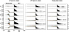 |
Fig. 1. Example of MCMC parameter chains for HARPS observations taken on November 11, 2019. The grouped columns represent the first burn-in chain (left), the second burn-in chain (middle), and the production chain (right), respectively. The left panels in each column show the sampled parameter values at each iterated step, where each colored line represent one walker and the black line represents the median of all 32 walkers. The parameter axis limits are set equal to the bounds of their uniform prior distributions (see Table 1). The right panels of each column show the ACF up to a lag of 400 steps. |
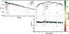 |
Fig. 2. Example of quality assessment for HARPS observations taken on November 11, 2019. Top panels: 60th spectral order magnitude, m60, as a function of airmass (left) and hour angle (right). The black line and gray area show the best fit and ±1σ interval for the estimated jitter. Data points are color-coded with their assessed quality shown in the colorbar. Points with a quality flag > 0.9 are accepted (circles), and the rest are rejected (squares). The magnitude error bars are smaller than the markers. Bottom panel: radial velocity as a function of hour angle. It should be noted that the displayed RVs are still uncorrected for differential extinction. |
The derived line slope of the airmass–magnitude relation, known as the extinction coefficient, was used to correct the RVs for differential extinction following the methodology of Collier Cameron et al. (2019). We thereafter impose a quality threshold, defined as the estimated probability of being a foreground point (see Eq. (3)), of 0.9 for all measurements. Figure 3 shows the overall improvement on the intraday rms. By correcting for differential extinction and rejecting low-quality measurements, we were able to improve the average daily rms by a factor of 1.63 and 1.96 for HARPS and HARPS-N, respectively. The higher average daily rms of HARPS compared to HARPS-N is attributed to its higher cadence (1 min instead of 5.5 min), enabling HARPS to resolve the p-mode oscillations of the Sun, which are averaged out in the HARPS-N measurements. We note that for this analysis, we also binned the HARPS measurements every 5.5 min, to equal the HARPS-N sampling and also mitigate the signal induced by stellar oscillations. After correction, we note that the binned HARPS data set reaches an average daily rms value of 0.69 m s−1, while the HARPS-N data set shows 0.53 m s−1. This is a significant difference, which is likely due to the fact that HARPS-N data are reduced with the recent ESPRESSO data reduction software (Dumusque et al. 2021), which is not the case for HARPS products. We are currently adapting this procedure for HARPS data. In Appendix A, the distribution of derived MCMC parameters are shown in Fig. A.1. Apart from c0 and μbg, which are both the scaled with the apparent magnitude of the Sun, none of the parameters indicate any correlation. The standard deviation of the background population, σbg, shows a bimodality since the sampling is unable to constrain the parameter on days without outliers on which its range is set by the bounds of the prior. Figure A.2 shows the number of outlier points per day, where HARPS points within 5.5 min from each other are only counted as one point to make the numbers comparable with HARPS-N. For most numbers of outliers per day, HARPS-N has a larger fraction of affected days than HARPS, which is indicative of the more humid and cloudy weather of La Palma compared to La Silla.
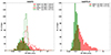 |
Fig. 3. Improvement of daily RV rms for HARPS (left panel) and HARPS-N (right panel). The histograms show the distribution of intraday rms scatter before (in red) and after (in green) removing points with quality flags < 0.9 and correcting for differential extinction with the fitted airmass-magnitude line parameters. For HARPS, we also binned the data every 5.5 min to equal the sampling of HARPS-N data and with it we averaged out the signal induced by stellar oscillations; the rms values of the binned HARPS data are shown in the fully colored histograms, and the rms values of the unbinned HARPS data are shown in the step histograms. The legend displays the average rms for the different distributions. Days with fewer than ten measurements remaining after imposing the quality flag threshold were rejected. For HARPS, the number of included days decreased from 376 to 326; for HARPS-N, the number of included days decreased from 745 to 644. |
The Python code implemented to compute the quality flags is publicly available on GitHub3, and can be easily adapted to any solar spectroscopic observations that have simultaneous recordings of the airmass and S/N.
4. Stellar components on sub-rotational timescales
Almost all kinds of ground-based astronomical data suffer from uneven temporal sampling due to poor observing conditions and limited allocated telescope time affecting our ability to collect data, but most importantly due to the diurnal cycle imposed by Earth’s rotation. And likewise, solar observations are subject to gaps due to nights. On long timescales (several months to years), these gaps introduce alias peaks in the Fourier spectra of temporal data (e.g., Dawson & Fabrycky 2010).
In Sect. 5, the observed stellar components are analyzed on all timescales, up to and including the rotational one. However, as an intermediate step, we demonstrate here the validity of our method by first applying it on a sub-rotational timescale for which alias peaks and instrumental long-term drifts are less significant.
4.1. Periodogram definition
We computed the Generalized Lomb-Scargle (GLS) periodogram (Zechmeister & Kürster 2009), which fits the RVs with a model composed of a linear combination of sinusoidal functions including constant offsets:
 (4)
(4)
where a(ν), b(ν), and c(ν) are the fitted coefficients, and ν are the sampled frequencies, ranging from 1/T, where T is the total time interval of the data, to the Nyquist frequency, 1/(2Δt), where Δt is the median of the sampled time steps, in increments of 1/T.
The GLS, as defined in Zechmeister & Kürster (2009), returns for each frequency the normalized χ2 of the best-fitted model. To calculate the power of the signal at each frequency, what is known as the velocity power spectrum (VPS), one calculates the summed squares of the sine and cosine terms:
 (5)
(5)
In order to obtain the VPSD, which is independent of the observing window, we multiplied the power by the effective length of the observing run, calculated as the inverse of the area under the window function (in units of power, see Kjeldsen et al. 2005). We note that our window function was obtained by computing the periodogram of a pure sine wave at the center-most sampled frequency. In Fig. 4, we observe that the power decays from lower to higher frequencies, in a behavior that is commonly attributed to granulation phenomena at several timescales; as the frequency increases, one identifies the emergence of the p-mode bump induced by multiple individual oscillation modes.
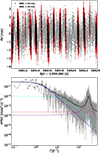 |
Fig. 4. HARPS RVs and VPSD between March 1 and 15, 2019. Top panel: HARPS RVs for which the sub-rotational components are analyzed. The original observations are shown as black dots with red error bars. The RVs recreated from the sum of all fitted VPSD components on an even time grid with the same cadence and end points as the observations are shown in gray. Bottom panel: velocity power spectral density of the observed RVs (in gray) and the modeled components (colored curves), consisting of photon noise (dotted red), oscillations (dashed purple), granulation (dash-dotted cyan) and supergranulation (dash-dotted blue). The sum of the models (solid black) is optimized with respect to the black circles, which correspond to the true VPSD averaged on logarithmically equidistant frequency steps. |
4.2. Analytical functions for power spectrum components
In order to recreate the RV contribution of each stellar component, we need to separate their power spectrum counterparts. This can be done by fitting the VPSD using analytical functions that capture the contribution of each type of stellar signal. Using analytical functions also allows us to reconstruct the RV of each component on an evenly sampled time grid. More generally, being able to reconstruct the RV on an evenly sampled time grid is crucial to test different observational strategies to mitigate stellar signal (e.g., Dumusque et al. 2011b; Dumusque 2016), or to estimate stellar contributions when searching for exoplanets (e.g., Dumusque et al. 2017; Meunier et al. 2010, 2019).
We followed the methodology of Lefebvre et al. (2008), and chose to fit the different stellar signal components with two types of analytical functions. The periodic components were fitted with a Lorentz function of the form
 (6)
(6)
where AL is the amplitude, Γ is the full-width at half-maximum (FWHM), and ν0 is the central frequency. The granulation phenomena were fitted with Harvey functions of the form
 (7)
(7)
where AH is the amplitude, τ is the characteristic timescale, and α is the power-law slope.
The fitting procedure was done with the Python module lmfit (Newville et al. 2020), which implements a Levenberg–Marquardt minimization. To reduce degeneracies from the large number of fitted parameters, we constrained our Harvey functions by setting α = 2 as in Lefebvre et al. (2008).
4.3. Recreated sub-rotational RV components
To demonstrate the validity of our method on sub-rotational timescales, we chose to recreate the contributing RV components as seen by HARPS for a duration of 15 days (i.e., roughly half the solar sidereal rotation period). We selected the part of the solar data set between March 1 and 15, 2019 (see Fig. 4). After computing the un-normalized VPSD, we binned the spectrum in 50 logarithmically equidistant frequency points and excluded the points at log10f < −0.5 where the sampling was too sparse. We then fit four components simultaneously: a constant photon noise level, one Lorentzian function for the envelope of oscillations, and two Harvey functions for granulation and supergranulation. The optimization was performed by minimizing the residual between the sum of all components and the binned true VPSD.
The individual VPSD components can be reconstructed into RVs using the following formula,
 (8)
(8)
where t are the recreated times in steps of Δt, ν and Δν are the frequencies and frequency steps of the VPSD, and ϕ(ν) is a randomly chosen phase between 0 and 2π. The upper panel of Fig. 4 shows the real RV data selected for the short timescale window, as well as the recreated RVs of the sum of the fitted components in the lower panel of the same figure. As indicated in the legend, both the real and recreated RVs have the same rms, indicating that the fitted components are able to capture all the significant stellar signals present on sub-rotational timescales. We were also able to recreate the individual RV contributions, as shown in Appendix B, where Fig. B.1 shows the RV amplitudes and rms values of all fitted components compared to the true total signal.
5. Stellar components up to rotational timescales
5.1. Combining the HARPS and HARPS-N data sets
The combination of HARPS measurements with minute-timescale cadence and HARPS-N measurements with long time coverage (3 years), enables us to resolve both low- and high-frequency stellar signals. By constructing a merged periodogram of the two data sets, we were able to simultaneously fit all the signal components. We chose to merge the periodograms in the frequency domain, rather than merging the RV data sets and performing a periodogram on the joint set. The reasoning behind this is that unless the RV sets are fully overlapping, their different cadences will cause some stellar signals to be inconsistent in the time domain, and furthermore, our cut-off for the sampled frequencies will be a poor estimate of the true Nyquist frequency.
The individual RV data sets were detrended on non-interfering timescales, adjusted for the different frequency domains each set was able to resolve. The HARPS measurements, which were used to resolve p-mode oscillations and small-scale granulation, were detrended with the inverse variance weighted daily mean in order to mitigate any day-to-day offsets induced by instability in daily wavelength solution derivation (e.g., Dumusque 2018; Trifonov et al. 2020; Dumusque et al. 2021). The HARPS-N measurements, which were used to resolve all other signals, that is to say, large-scale granulation and rationally modulated activity, were detrended with a 100-day rolling mean in order to mitigate the 11-year magnetic activity cycle and instrumental long-term drifts. Figure 5 shows the entire RV time series of both instruments before and after detrending.
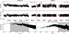 |
Fig. 5. Total RV time series and VPS for HARPS and HARPS-N. Top: radial velocity time series. Middle: HARPS-N RVs detrended by a 100-day rolling mean, and HARPS RVs detrended by a weighted daily mean. Bottom: generalized Lomb-Scargle periodogram where the gray regions are merged together. |
The VPS and VPSD were computed in the same way as in Sect. 4 on the detrended RVs. The VPSDs were then combined together by merging the HARPS-N VPSD in the frequency range f = 10−2 − 101 d−1 with the HARPS VPSD in the frequency range f = 10−1−fmax d−1, where fmax is the highest resolved frequency with HARPS. The lower limit was set by the 100-day detrending imposed on the HARPS-N RVs, and the frequency at which the VPSDs were merged was taken to be a rough mid-point between the optimal frequency windows of each detrended data set. We fit the same signal components to the VPSD as before, namely photon noise, oscillations, granulation, and supergranulation, in addition to the rotational components.
5.2. Recreated rotational RV components
The sub-rotational components were recreated as described in Sect. 4, but on a different timescale. Since the frequency scale was bounded by the total time span of the HARPS-N observations and the cadence of the HARPS observations, we chose here to recreate the components on the timescale and cadence of only the HARPS observations. This is because the longer the timescale selected, the greater the number of computed time points and the greater the number of frequencies over which the summation is performed in Eq. (8), significantly increasing the nonlinear computational time. The time span of the HARPS observations is nearly two years, and thus it is large enough to cover many rotational periods.
The rotational contributions are quasi-periodic, with a periodicity of the sidereal rotation period of the Sun of about 27 days and its harmonics. We chose to model the fundamental and first two harmonics, and fit each component with a Lorentz function, alike the p-mode oscillations. To reduce the number of free parameters, we imposed that the frequencies of the first and second harmonics were twice and thrice the value of the fundamental.
The rotational harmonics with central frequencies ν0, i (i = 0, 1, 2) convolved with the window functions of HARPS-N, which has strong daily alias peaks due to solar observations being restricted to daytime, will create aliases in the VPSD at frequencies
 (9)
(9)
where m is an integer number. Since the central frequencies of the rotational peaks are much smaller than unity, the aliases appear at roughly ν ≈ 1, 2, … d−1. The forest of peaks around the two primary aliases were also fitted with Lorentzian functions with fixed centers. Finally, since some of the spectral power was allocated from the rotational peaks to the aliases, we attempted to redistribute the alias power when recreating the rotational RV contribution. This was executed by first summing over the alias Lorentizians evaluated at the frequencies corresponding to the recreated time points. The summed alias VPSD was then proportionally divided between the rotational peaks, where each peak received a fraction:
 (10)
(10)
where the index i corresponds the ith rotational harmonic with amplitude Ai. The redistributed power was added at  , the sampled frequency closest to the central frequency of the ith rotational component. The customization of Eq. (8) for the rotational contribution thus becomes
 (11)
(11)
The alias components were not reconstructed in the same way as the other components. This is because although they might contribute to the total rms in agreement with the observed scatter, their reconstructed RVs will have periodicities that are too short, since they will be related to the frequency of the sampling gaps instead of the stellar signal from which they originate.
The fitted VPSD components are shown in Fig. 6, and the best-fit values of the coefficients of the analytical expressions are listed in Table 2, together with their estimated uncertainties. The recreated individual RV components are shown in Fig. 7, allowing for the peak-to-peak comparison of various signals. The bottom right panel shows the recreated RVs obtained from the sum of all components, which is able to capture similar structure and scatter as the true total signal. Table 3 displays the RV rms of both the observed data sets and the recreated components. We note that on the original HARPS data, we also fitted for a linear, long-term trend to remove any signal induced by the solar magnetic cycle. The RV rms obtained on HARPS measurements, 1.58 m s−1, is comparable to that obtained with HARPS-N once the long-term trend is removed (1.37 m s−1) and the contribution of the unresolved oscillations are added ( ).
).
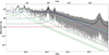 |
Fig. 6. Stellar signal components fitted to the combined HARPS and HARPS-N VPSD (solid gray curve). The dotted red curve shows the photon-noise constant. The dashed curves represent Lorentzian functions for oscillations (purple), rotation and its harmonics (green), and aliases (black), whereas dash-dotted curves represent Harvey functions for granulation (cyan) and supergranulation (blue). The solid black curve is the sum of all components, which was fitted with respect to the binned VPSD (black circles). |
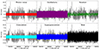 |
Fig. 7. Recreated RV components up to rotational timescales. Individual RV contributions are from the stellar signals fitted in the VPSD of Fig. 6. The components are indicated in the top of each subplot and the RV points are color-coded according to the curve colors in Fig. 6. The true total signal from the HARPS RVs (without error bars) with a linear drift subtracted is shown in gray for comparison. |
Radial velocity rms contributions.
Although the total recreated signal is visually similar in amplitude and modulation, its rms value is about 27 cm s−1 lower than that of the HARPS data, on whose timescale the RVs were simulated. We believe this discrepancy could be due to several factors associated with attempting to extend this kind of analysis to rotational timescales. The most uncertain among them is the validity of our method when used to combine correlated contributions, such as the rotational harmonics. On sub-rotational timescales, the validity of using random phases when recreating p-mode oscillations and granulation phenomena was motivated by their stochastic, and thus independent, nature. However, attributing the rotational harmonics random phases as well could lead to deconstructive interference at times when they are behaving more coherently in the real observations. Another possibly impacting factor is the influence of the solar magnetic cycle, which does not only affect the RVs with a long-term drift (which we corrected for by detrending), but also the intrinsic amplitudes and characteristic timescales of the modeled stellar signals with time.
6. Discussion and conclusions
An important step toward better understanding the origin and mechanisms of solar and stellar variability is accurately measuring the magnitude and timescales of various activity sources, allowing subsequent models to build on better constraints from observations. In this study we have assessed the quality of high-precision, high-cadence solar RVs taken with the HARPS and HARPS-N spectrographs to build a near-continuous data set suitable for investigating the typical stellar signals that are present at all timescales up to the stellar rotation period. We have analyzed the merged VPSDs of both instruments to highlight the best-resolved features from each one.
We have been able to show that using fairly simple analytical functions, one can easily estimate the RV budget of various stellar signals at different frequency ranges. On sub-rotational timescales, we were able to fully capture the significant contributions of p-mode oscillations and granulation phenomena. We find that solar oscillations induce a RV rms of 0.73 m s−1, which is fully compatible with the solar estimation performed in Chaplin et al. (2019, see Fig. 3). Regarding granulation and supergranulation, we find RV rms contributions at the level of 0.31 and 0.68 m s−1, respectively. For granulation, the derived value is significantly smaller than the outcome of the simulation performed by Meunier et al. (2015), who found 0.8 m s−1. The same study also simulated supergranulation and the authors estimated a contribution to an RV rms level between 0.28 and 1.12 m s−1. The value that we found when analyzing solar data is in the middle of this range, and therefore it is fully compatible. We note that the discrepancy between the granulation found in observations and simulations could be due to different ranges in considered frequency, since granulation induces a signal over a large range of frequencies.
We were also able to extend our analysis up to rotational timescales through the inclusion of quasi-periodic peaks originating from active magnetic regions corotating with the solar surface. By modeling both the most prominent harmonics and their associated alias peaks due to the uneven time sampling, and proportionally redistributing the integrated alias power to the central frequencies of the rotational components, we were able to reach similar peak-to-peak variations and slightly underestimated RV rms when comparing the true signals and the sum of our fitted components. In our analysis, we find that rotational modulation induces an RV rms of 0.74 m s−1 on the Sun during the minimum of its activity cycle.
The contribution of oscillations, supergranulation, and rotational activity are at very similar RV rms levels. However, they do not contribute equally when searching for exoplanets. Indeed, due to the short timescale of oscillations, their impact can be reduced to levels lower than 0.1 m s−1 by imposing exposure times longer than their typical timescale (e.g., Chaplin et al. 2019). This is not the case for supergranulation, which evolves with a timescale of up to several days. Although taking several measurements per night can reduce the impact of this stellar signal (Dumusque et al. 2011b), Meunier et al. (2015) show that even after averaging data over 5 days, the RV rms is above 0.17 m s−1. Regarding rotational activity, this stellar signal is even more complex to handle as we can no longer average out data to mitigate its impact.
Since our modeling of stellar signals can be used to generate RVs with a continuous and extremely high cadence, any realistic sampling can be reproduced, and therefore the results of this paper can be used to test observational strategies, how they can mitigate stellar signals, and influence the detection of exoplanets. It would be possible, for example, to optimize observations of further RV surveys aiming to detect Earth analogs orbiting very quiet stars.
As solar telescopes equipped with high-resolution spectrographs continue to gather near-continuous data, similar studies can be extended to cover one or several magnetic cycles. Future work could also investigate the temporal evolution of recreated RV components by splitting the available data according to the minima or maxima of such cycles.
http://exoplanet.eu (as of October 10, 2022).
Acknowledgments
We thank the anonymous referee for valuable comments which helped improve the quality of the manuscript. This work has been carried out within the framework of the National Centre of Competence in Research PlanetS supported by the Swiss National Science Foundation under grants 51NF40_182901 and 51NF40_205606. The authors acknowledge the financial support of the SNSF. This project has received funding from the European Research Council (ERC) under the European Union’s Horizon 2020 research and innovation program (grant agreement SCORE No. 851555). NCS acknowledges the support from the European Research Council through the grant agreement 101052347 (FIERCE). This work was supported by FCT – Fundação para a Ciência e a Tecnologia through national funds and by FEDER through COMPETE2020 – Programa Operacional Competitividade e Internacionalização by these grants: UIDB/04434/2020; UIDP/04434/2020.
References
- Al Moulla, K., Dumusque, X., Cretignier, M., et al. 2022, A&A, 664, A34 [NASA ADS] [CrossRef] [EDP Sciences] [Google Scholar]
- Bauer, F. F., Reiners, A., Beeck, B., et al. 2018, A&A, 610, A52 [NASA ADS] [CrossRef] [EDP Sciences] [Google Scholar]
- Bouguer, P. 1729, Essai d’Optique sur la gradation de la Lumiere (Paris: C. Jombert) [Google Scholar]
- Cegla, H. M., Shelyag, S., Watson, C. A., et al. 2013, ApJ, 763, 95 [NASA ADS] [CrossRef] [Google Scholar]
- Cegla, H. M., Watson, C. A., Shelyag, S., et al. 2019, ApJ, 879, 55 [NASA ADS] [CrossRef] [Google Scholar]
- Chaplin, W. J., Cegla, H. M., Watson, C. A., et al. 2019, AJ, 157, 163 [NASA ADS] [CrossRef] [Google Scholar]
- Christensen-Dalsgaard, J. 2004, Sol. Phys., 220, 137 [Google Scholar]
- Collier Cameron, A., Mortier, A., Phillips, D., et al. 2019, MNRAS, 487, 1082 [Google Scholar]
- Collier Cameron, A., Ford, E. B., Shahaf, S., et al. 2021, MNRAS, 505, 1699 [NASA ADS] [CrossRef] [Google Scholar]
- Dawson, R. I., & Fabrycky, D. C. 2010, ApJ, 722, 937 [Google Scholar]
- de Beurs, Z. L., Vanderburg, A., Shallue, C. J., et al. 2022, AJ, 164, 49 [NASA ADS] [CrossRef] [Google Scholar]
- Del Moro, D. 2004, A&A, 428, 1007 [NASA ADS] [CrossRef] [EDP Sciences] [Google Scholar]
- Del Moro, D., Berrilli, F., Duvall, T. L., Jr, et al. 2004, Sol. Phys., 221, 23 [CrossRef] [Google Scholar]
- Dumusque, X. 2016, A&A, 593, A5 [NASA ADS] [CrossRef] [EDP Sciences] [Google Scholar]
- Dumusque, X. 2018, A&A, 620, A47 [NASA ADS] [CrossRef] [EDP Sciences] [Google Scholar]
- Dumusque, X., Santos, N. C., Udry, S., et al. 2011a, A&A, 527, A82 [NASA ADS] [CrossRef] [EDP Sciences] [Google Scholar]
- Dumusque, X., Udry, S., Lovis, C., et al. 2011b, A&A, 525, A140 [NASA ADS] [CrossRef] [EDP Sciences] [Google Scholar]
- Dumusque, X., Boisse, I., & Santos, N. C. 2014, ApJ, 796, 132 [NASA ADS] [CrossRef] [Google Scholar]
- Dumusque, X., Glenday, A., Phillips, D. F., et al. 2015, ApJ, 814, L21 [Google Scholar]
- Dumusque, X., Borsa, F., Damasso, M., et al. 2017, A&A, 598, A133 [NASA ADS] [CrossRef] [EDP Sciences] [Google Scholar]
- Dumusque, X., Cretignier, M., Sosnowska, D., et al. 2021, A&A, 648, A103 [NASA ADS] [CrossRef] [EDP Sciences] [Google Scholar]
- Ervin, T., Halverson, S., Burrows, A., et al. 2022, AJ, 163, 272 [NASA ADS] [CrossRef] [Google Scholar]
- Ford, E. B. 2006, ApJ, 642, 505 [Google Scholar]
- Foreman-Mackey, D. 2014, https://doi.org/10.5281/zenodo.15856 [Google Scholar]
- Foreman-Mackey, D., Hogg, D. W., Lang, D., et al. 2013, PASP, 125, 306 [NASA ADS] [CrossRef] [Google Scholar]
- Goldreich, P., & Keeley, D. A. 1977, ApJ, 212, 243 [NASA ADS] [CrossRef] [Google Scholar]
- Haywood, R. D., Collier Cameron, A., Unruh, Y. C., et al. 2016, MNRAS, 457, 3637 [Google Scholar]
- Herrero, E., Ribas, I., Jordi, C., et al. 2016, A&A, 586, A131 [NASA ADS] [CrossRef] [EDP Sciences] [Google Scholar]
- Hogg, D. W., Bovy, J., & Lang, D. 2010, ArXiv e-prints [arXiv:1008.4686] [Google Scholar]
- Kjeldsen, H., & Bedding, T. R. 1995, A&A, 293, 87 [NASA ADS] [Google Scholar]
- Kjeldsen, H., Bedding, T. R., Butler, R. P., et al. 2005, ApJ, 635, 1281 [NASA ADS] [CrossRef] [Google Scholar]
- Langellier, N., Milbourne, T. W., Phillips, D. F., et al. 2021, AJ, 161, 287 [NASA ADS] [CrossRef] [Google Scholar]
- Lefebvre, S., García, R. A., Jiménez-Reyes, S. J., et al. 2008, A&A, 490, 1143 [NASA ADS] [CrossRef] [EDP Sciences] [Google Scholar]
- Lindegren, L., & Dravins, D. 2003, A&A, 401, 1185 [NASA ADS] [CrossRef] [EDP Sciences] [Google Scholar]
- Maldonado, J., Phillips, D. F., Dumusque, X., et al. 2019, A&A, 627, A118 [NASA ADS] [CrossRef] [EDP Sciences] [Google Scholar]
- Mayor, M., & Queloz, D. 1995, Nature, 378, 355 [Google Scholar]
- Mayor, M., Pepe, F., Queloz, D., et al. 2003, The Messenger, 114, 20 [NASA ADS] [Google Scholar]
- Meunier, N., Desort, M., & Lagrange, A.-M. 2010, A&A, 512, A39 [NASA ADS] [CrossRef] [EDP Sciences] [Google Scholar]
- Meunier, N., Lagrange, A.-M., Borgniet, S., et al. 2015, A&A, 583, A118 [NASA ADS] [CrossRef] [EDP Sciences] [Google Scholar]
- Meunier, N., Lagrange, A.-M., Boulet, T., et al. 2019, A&A, 627, A56 [NASA ADS] [CrossRef] [EDP Sciences] [Google Scholar]
- Milbourne, T. W., Haywood, R. D., Phillips, D. F., et al. 2019, ApJ, 874, 107 [Google Scholar]
- Milbourne, T. W., Phillips, D. F., Langellier, N., et al. 2021, ApJ, 920, 21 [NASA ADS] [CrossRef] [Google Scholar]
- Newville, M., Otten, R., Nelson, A., et al. 2020, https://doi.org/10.5281/zenodo.3814709 [Google Scholar]
- Pesnell, W. D., Thompson, B. J., & Chamberlin, P. C. 2012, Sol. Phys., 275, 3 [Google Scholar]
- Phillips, D. F., Glenday, A. G., Dumusque, X., et al. 2016, in Advances in Optical and Mechanical Technologies for Telescopes and Instrumentation II, SPIE Conf. Ser., 9912, 99126Z [Google Scholar]
- Saar, S. H., & Donahue, R. A. 1997, ApJ, 485, 319 [Google Scholar]
- Schrijver, C. J., & Zwaan, C. 2000, Solar and Stellar Magnetic Activity, 1st edn. (Cambridge: Cambridge University Press) [Google Scholar]
- Trifonov, T., Tal-Or, L., Zechmeister, M., et al. 2020, A&A, 636, A74 [NASA ADS] [CrossRef] [EDP Sciences] [Google Scholar]
- Zechmeister, M., & Kürster, M. 2009, A&A, 496, 577 [CrossRef] [EDP Sciences] [Google Scholar]
Appendix A: Statistics of MCMC parameters and outliers
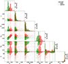 |
Fig. A.1. Corner plot of MCMC parameters. The subplots show the distribution of the daily fitted parameters described in Table 1, for both HARPS (green points) and HARPS-N (red points). The top subplot of each column shows the histogram in units of fraction of the total number of days per instrument. The dashed lines indicate the median values, and the contour curves represent the ±1σ kernel densities. |
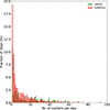 |
Fig. A.2. Outlier statistics. The histograms show the distribution of the number of outliers, i.e., points with a quality flag < 0.9, per day for HARPS (green) and HARPS-N (red). The histograms are binned between one and 100 outliers per day in steps of one. The fraction of days is relative to the number of days observed with each instrument. For HARPS and HARPS-N, 47.3% and 76.1%, respectively, of all observed days have at least one outlier. |
Appendix B: Radial velocity components on sub-rotational timescales
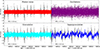 |
Fig. B.1. Recreated RV components on sub-rotational timescales. Individual RV contributions are from the stellar signals fitted in the VPSD of Fig. 4. The components are indicated in the top of each subplot and the RV points are color-coded according to the curve colors in Fig. 4. The rms of each component is shown in the lower left legend in each subplot. The true total signal (without error bars) is shown in gray for comparison. |
All Tables
All Figures
|
Fig. 1. Example of MCMC parameter chains for HARPS observations taken on November 11, 2019. The grouped columns represent the first burn-in chain (left), the second burn-in chain (middle), and the production chain (right), respectively. The left panels in each column show the sampled parameter values at each iterated step, where each colored line represent one walker and the black line represents the median of all 32 walkers. The parameter axis limits are set equal to the bounds of their uniform prior distributions (see Table 1). The right panels of each column show the ACF up to a lag of 400 steps. |
| In the text | |
|
Fig. 2. Example of quality assessment for HARPS observations taken on November 11, 2019. Top panels: 60th spectral order magnitude, m60, as a function of airmass (left) and hour angle (right). The black line and gray area show the best fit and ±1σ interval for the estimated jitter. Data points are color-coded with their assessed quality shown in the colorbar. Points with a quality flag > 0.9 are accepted (circles), and the rest are rejected (squares). The magnitude error bars are smaller than the markers. Bottom panel: radial velocity as a function of hour angle. It should be noted that the displayed RVs are still uncorrected for differential extinction. |
| In the text | |
|
Fig. 3. Improvement of daily RV rms for HARPS (left panel) and HARPS-N (right panel). The histograms show the distribution of intraday rms scatter before (in red) and after (in green) removing points with quality flags < 0.9 and correcting for differential extinction with the fitted airmass-magnitude line parameters. For HARPS, we also binned the data every 5.5 min to equal the sampling of HARPS-N data and with it we averaged out the signal induced by stellar oscillations; the rms values of the binned HARPS data are shown in the fully colored histograms, and the rms values of the unbinned HARPS data are shown in the step histograms. The legend displays the average rms for the different distributions. Days with fewer than ten measurements remaining after imposing the quality flag threshold were rejected. For HARPS, the number of included days decreased from 376 to 326; for HARPS-N, the number of included days decreased from 745 to 644. |
| In the text | |
|
Fig. 4. HARPS RVs and VPSD between March 1 and 15, 2019. Top panel: HARPS RVs for which the sub-rotational components are analyzed. The original observations are shown as black dots with red error bars. The RVs recreated from the sum of all fitted VPSD components on an even time grid with the same cadence and end points as the observations are shown in gray. Bottom panel: velocity power spectral density of the observed RVs (in gray) and the modeled components (colored curves), consisting of photon noise (dotted red), oscillations (dashed purple), granulation (dash-dotted cyan) and supergranulation (dash-dotted blue). The sum of the models (solid black) is optimized with respect to the black circles, which correspond to the true VPSD averaged on logarithmically equidistant frequency steps. |
| In the text | |
|
Fig. 5. Total RV time series and VPS for HARPS and HARPS-N. Top: radial velocity time series. Middle: HARPS-N RVs detrended by a 100-day rolling mean, and HARPS RVs detrended by a weighted daily mean. Bottom: generalized Lomb-Scargle periodogram where the gray regions are merged together. |
| In the text | |
|
Fig. 6. Stellar signal components fitted to the combined HARPS and HARPS-N VPSD (solid gray curve). The dotted red curve shows the photon-noise constant. The dashed curves represent Lorentzian functions for oscillations (purple), rotation and its harmonics (green), and aliases (black), whereas dash-dotted curves represent Harvey functions for granulation (cyan) and supergranulation (blue). The solid black curve is the sum of all components, which was fitted with respect to the binned VPSD (black circles). |
| In the text | |
|
Fig. 7. Recreated RV components up to rotational timescales. Individual RV contributions are from the stellar signals fitted in the VPSD of Fig. 6. The components are indicated in the top of each subplot and the RV points are color-coded according to the curve colors in Fig. 6. The true total signal from the HARPS RVs (without error bars) with a linear drift subtracted is shown in gray for comparison. |
| In the text | |
|
Fig. A.1. Corner plot of MCMC parameters. The subplots show the distribution of the daily fitted parameters described in Table 1, for both HARPS (green points) and HARPS-N (red points). The top subplot of each column shows the histogram in units of fraction of the total number of days per instrument. The dashed lines indicate the median values, and the contour curves represent the ±1σ kernel densities. |
| In the text | |
|
Fig. A.2. Outlier statistics. The histograms show the distribution of the number of outliers, i.e., points with a quality flag < 0.9, per day for HARPS (green) and HARPS-N (red). The histograms are binned between one and 100 outliers per day in steps of one. The fraction of days is relative to the number of days observed with each instrument. For HARPS and HARPS-N, 47.3% and 76.1%, respectively, of all observed days have at least one outlier. |
| In the text | |
|
Fig. B.1. Recreated RV components on sub-rotational timescales. Individual RV contributions are from the stellar signals fitted in the VPSD of Fig. 4. The components are indicated in the top of each subplot and the RV points are color-coded according to the curve colors in Fig. 4. The rms of each component is shown in the lower left legend in each subplot. The true total signal (without error bars) is shown in gray for comparison. |
| In the text | |
Current usage metrics show cumulative count of Article Views (full-text article views including HTML views, PDF and ePub downloads, according to the available data) and Abstracts Views on Vision4Press platform.
Data correspond to usage on the plateform after 2015. The current usage metrics is available 48-96 hours after online publication and is updated daily on week days.
Initial download of the metrics may take a while.