| Issue |
A&A
Volume 663, July 2022
|
|
|---|---|---|
| Article Number | A22 | |
| Number of page(s) | 29 | |
| Section | Extragalactic astronomy | |
| DOI | https://doi.org/10.1051/0004-6361/202142172 | |
| Published online | 04 July 2022 | |
High resolution spectral imaging of CO(7–6), [CI](2–1), and continuum of three high-z lensed dusty star-forming galaxies using ALMA
1
Aix Marseille Univ., CNRS, CNES, LAM, Marseille, France
e-mail: This email address is being protected from spambots. You need JavaScript enabled to view it.
2
NHFP Hubble Fellow, University of Texas at Austin, 2515 Speedway Stop C1400, Austin, TX, 78712
USA
3
Núcleo de Astronomía, Facultad de Ingeniería y Ciencias, Universidad Diego Portales, Av. Ejército 441, Santiago, Chile
4
Department of Astronomy, University of Illinois at Urbana-Champaign, 1002 West Green St., Urbana, IL, 61801
USA
5
Center for AstroPhysical Surveys, National Center for Supercomputing Applications, Urbana, IL, 61801
USA
6
Department of Physics and Astronomy, University of British Columbia, 6225 Agricultural Road, Vancouver, V6T 1Z1
Canada
7
National Research Council, Herzberg Astronomy and Astrophysics, 5071 West Saanich Road, Victoria, V9E 2E7
Canada
8
Department of Physics and Atmospheric Science, Dalhousie University, 6310 Coburg Road, B3H 4R2 Halifax, Canada
9
European Southern Observatory, Karl Schwarzschild Straße 2, 85748 Garching, Germany
10
Department of Astronomy, University of Florida, 211 Bryant Space Sciences Center, Gainesville, FL, 32611
USA
11
Center for Computational Astrophysics, Flatiron Institute, 162 Fifth Avenue, New York, NY, 10010
USA
12
Département de Physique, Université de Montréal, Montreal, Quebec, H3T 1J4
Canada
13
Steward Observatory, University of Arizona, 933 North Cherry Avenue, Tucson, AZ, 85721
USA
14
Department of Physics and Astronomy, University of California, Los Angeles, CA, 90095-1547
USA
15
University of Florida Informatics Institute, 432 Newell Drive, CISE Bldg E251, Gainesville, FL, 32611
USA
16
Cosmic Dawn Center (DAWN), DTU-Space, Technical University of Denmark, Elektrovej 327, 2800 Kgs. Lyngby, Denmark
17
Department of Physics, University of Illinois Urbana-Champaign, 1110 West Green Street, Urbana, IL, 61801
USA
18
Max-Planck-Institut für Radioastronomie, Auf dem Hugel 69, 53121 Bonn, Germany
Received:
8
September
2021
Accepted:
15
March
2022
Abstract
High-redshift dusty star-forming galaxies with very high star formation rates (500−3000 M⊙ yr−1) are key to understanding the formation of the most extreme galaxies in the early Universe. Characterising the gas reservoir of these systems can reveal the driving factor behind the high star formation. Using molecular gas tracers such as, high-J CO lines, neutral carbon lines, and the dust continuum, we can estimate the gas density and radiation field intensity in their interstellar media. In this paper, we present high resolution (∼0.4″) observations of CO(7−6), [CI](2−1), and dust continuum of three lensed galaxies from the South pole telescope – sub-millimetre galaxies (SPT-SMG) sample at z ∼ 3 with the Atacama Large Millimetre/submillimetre Array. Our sources have high intrinsic star formation rates (> 850 M⊙ yr−1) and rather short depletion timescales (< 100 Myr). Based on the L[CI](2−1)/LCO(7 − 6) and L[CI](2−1)/LIR ratios, our galaxy sample has similar radiation field intensities and gas densities compared to other submillimetre galaxies. We performed visibility-based lens modelling on these objects to reconstruct the kinematics in the source plane. We find that the cold gas masses of the sources are compatible with simple dynamical mass estimates using ULIRG-like values of the CO-H2 conversion factor αCO, but not Milky Way-like values. We find diverse source kinematics in our sample: SPT0103−45 and SPT2147−50 are likely rotating disks, while SPT2357−51 is possibly a major merger. The analysis presented in the paper could be extended to a larger sample to determine better statistics of morphologies and interstellar medium properties of high-z dusty star-forming galaxies.
Key words: galaxies: high-redshift / galaxies: evolution / galaxies: ISM / galaxies: kinematics and dynamics / galaxies: star formation / submillimeter: galaxies
© G. Gururajan et al. 2022
 Open Access article, published by EDP Sciences, under the terms of the Creative Commons Attribution License (https://creativecommons.org/licenses/by/4.0), which permits unrestricted use, distribution, and reproduction in any medium, provided the original work is properly cited.
1. Introduction
Large populations of dusty star-forming galaxies (DSFGs) have been observed in the high-redshift Universe (e.g. Greve et al. 2012; Casey et al. 2014; da Cunha et al. 2015). They can host star-formation rates (SFR) as high as ∼1000 M⊙ yr−1. DSFGs account for roughly ∼20% of the star formation density and ∼10% of the molecular gas content at z ∼ 1 − 5 (Swinbank et al. 2014). Typically selected at infrared and millimetre wavelengths, DSFGs are bright in submillimetre wavelengths as their ultraviolet and optical emission is mainly absorbed by the dust and re-emitted in the rest-frame far-infrared (redshifted to the submillimetre). The rapid star formation in these systems seems to be driven by not only massive gas reservoirs, but also an increase in the star formation efficiency, SFE ≡ SFR/MH2, or equivalently, short gas depletion timescales tdep ≡ MH2/SFR (e.g. Tacconi et al. 2013; Dessauges-Zavadsky et al. 2015; Béthermin et al. 2015; Aravena et al. 2016). Understanding the formation of such systems could provide key insights into the evolution of the most extreme galaxies at early times.
At 1 < z < 4, most massive galaxies have SFEs similar to local spirals, but with larger gas reservoirs (e.g. Tacconi et al. 2010; Daddi et al. 2010a; Saintonge et al. 2013; Dessauges-Zavadsky et al. 2015; Béthermin et al. 2015) possibly driven by rapid accretion of cold gas from the cosmic web (e.g. Dekel et al. 2009; Kleiner et al. 2017; Kretschmer et al. 2020; Chun et al. 2020). However, the most rapidly star-forming systems (SFR > 500 M⊙ yr−1) usually have both a large gas reservoir and a high SFE (Harris et al. 2012; Ivison et al. 2012; Tan et al. 2014; Aravena et al. 2016; Ciesla et al. 2020; Jarugula et al. 2021). These high SFEs also seem to be associated with high dense gas fractions (Oteo et al. 2017; Béthermin et al. 2018). Measuring the composition and physical properties of the gas reservoir is thus key to understanding the physical mechanisms leading to the extreme star formation observed in DSFGs.
The observed dust continuum of DSFGs can be used to derive the total infrared (IR) luminosity (LIR), which can then be used to estimate the obscured SFR (Kennicutt 1998; Kennicutt & Evans 2012). The contents of the Interstellar medium (ISM) gas reservoirs can also be observed and quantified using various tracers. The carbon monoxide (CO) emission lines and particularly the low-J transitions are common tracers of the molecular H2 gas (e.g. Greve et al. 2005; Solomon & Vanden Bout 2005; Omont 2007; Carilli & Walter 2013; Bothwell et al. 2013; Bolatto et al. 2013). Measuring the low-J CO emission thereby provides a good estimate of the total molecular gas mass of the system (e.g. Daddi et al. 2010a; Genzel et al. 2010). Together, the low-J CO lines and the IR luminosity can then be used to estimate the SFE. High-J (J ≥ 7) CO lines trace warm and dense molecular gas in active star-forming regions (e.g. Weiß et al. 2005, 2007; Carilli & Walter 2013; Yang et al. 2017).
Measurements of the molecular gas mass through low-J CO lines are limited by the need to assume αCO, the molecular gas mass-to-CO luminosity conversion factor, which is known to vary with density and metallicity (Bolatto et al. 2013), but it can also be affected by mergers (e.g. Daddi et al. 2010b; Genzel et al. 2010). At z > 3, the CO(1−0) line is difficult to detect, so most studies focus on the detection of J ≥ 3 transitions. Because αCO is based on the CO(1−0) transition, these studies must then assume or estimate the CO line excitation in order to convert the observed line luminosity to the luminosity of the ground state transition (Narayanan & Krumholz 2014; Tunnard & Greve 2016). The CO line excitation depends on the gas temperature and density, which in turn also influence many other aspects of galaxies such as the instantaneous SFR.
Alternatively, the molecular gas mass can also be traced by the two neutral carbon fine structure lines, CI(3P2 − 3P1) and CI(3P1 − 3P0), henceforth the [CI](2−1) and [CI](1−0) lines, respectively. Although initially, the [CI] emission was thought to be arising only from a thin layer between the molecular carbon and the ionised carbon regions of the photodissociation region (PDR) (Langer 1976; Tielens & Hollenbach 1985), subsequent detection of [CI] and CO in the galactic molecular clouds, revealed that the [CI] was more widely distributed across the cloud (Keene et al. 1985). This began the new prospects of using [CI] as a tracer of extended molecular gas in the galaxies (Papadopoulos et al. 2004; Papadopoulos & Greve 2004).
Unlike the CO transitions, [CI] is optically thin and thus a good tracer of the gas mass if the carbon abundance, XCI is known or can be assumed (Bisbas et al. 2015; Dunne et al. 2021). It is also less affected by physical conditions like cosmic rays, unlike CO(1−0) (e.g. Weiß et al. 2003; Papadopoulos et al. 2004; Papadopoulos & Greve 2004; Walter et al. 2011; Tomassetti et al. 2014; Bothwell et al. 2017) and the line excitation has only a small impact on the derived gas mass for typical line excitation temperatures (e.g. Walter et al. 2011; Harrington et al. 2021).
Various analyses have been conducted on the high-J CO/[CI] line ratios (e.g. Yang et al. 2017; Andreani et al. 2018; Valentino et al. 2020). This ratio has shown to be a good tracer of the density of the ISM. Andreani et al. (2018) advocate that [CI](2−1)-dominated objects (CO(7−6)/[CI](2−1) ≤ 1) are extended gas-rich disk structures with modest star formation efficiencies, while CO(7−6)-bright objects are predominately merging systems. A significant fraction of DSFGs are shown to have multiple components (e.g. Hodge et al. 2013; Karim et al. 2013) often interpreted as evidence of merging systems. The CO/[CI] ratio could be an alternative diagnostic tool for the merging status of a DSFG.
High-resolution imaging of DSFGs typically requires long integration times. Surveys like ALMA-ALPINE (Le Fèvre et al. 2020; Béthermin et al. 2020; Faisst et al. 2020) observed the very bright [CII] line emission, but even this survey could only marginally spatially resolve the sources. CO samples have mainly been observed at z < 3 and only a very small fraction of them are spatially resolved (e.g. Tacconi et al. 2013; Dessauges-Zavadsky et al. 2015; Magdis et al. 2017). In contrast, gravitationally lensed samples can provide better resolution due to the lensing magnification in shorter observation time (e.g. Bussmann et al. 2015; Spilker et al. 2016). Many samples of lensed DSFGs have been built in the recent years using the Herschel/SPIRE (Negrello et al. 2010; Bussmann et al. 2015), Atacama Cosmology Telescope (ACT, Marsden et al. 2014), South Pole Telescope (SPT, Vieira et al. 2010; Carlstrom et al. 2011) and Planck (Cañameras et al. 2015) surveys. Large follow-up campaigns were then performed using interferometers such as the Atacama Large Millimeter/sub-millimeter Array (ALMA), NOrthern Extended Millimeter Array (NOEMA) and Sub-Millimeter Array (SMA).
In this paper, we take advantage of the gravitational lensing magnification of three lensed DSFGs from the SPT sample (Vieira et al. 2013; Spilker et al. 2016; Strandet et al. 2016; Reuter et al. 2020) in order to study the resolved properties of the ISM using high resolution spectral and spatial imaging of the CO(7−6), [CI](2−1) line, and the dust continuum emission with ALMA. With this data, we analyse the kinematics and morphology of the sources. We also explore the resolved ISM properties of our sources through line and continuum ratio analysis. We perform lens modelling of the line and continuum emission of our sources to understand their source-plane morphology, explore potential differential magnification effects (e.g. Serjeant 2012; Hezaveh et al. 2012) and reconstruct the intrinsic kinematics of the sources.
The paper is structured as follows. Section 2 presents our sample and the ALMA observations of the sources. The data reduction and imaging are described in Sect. 3. The observed source morphologies and the spectra of the lines are described in Sect. 4. Section 5 presents the analysis of the kinematics of our sample. The lens modelling is presented in Sect. 6. The resolved line and continuum ratio analyses are presented in Sect. 7. Finally, a brief discussion and conclusion of our analyses are presented in Sects. 8 and 9, respectively.
Throughout this paper, we adopt a ΛCDM cosmology with Ωm = 0.3, ΩΛ = 0.7 and H0 = 70 km s−1 Mpc−1 and a Chabrier (2003) initial mass function (IMF).
2. Sample and observations
2.1. SPT-SMG APEX/SEPIA [CI] sample
Our sample of three galaxies was selected from an initial programme (PIs: Béthermin and Strandet, project number: 097.A-0973) targeting CO(7−6) and [CI](2−1) in 8 DSFGs from the SPT-SMG sample with the APEX/SEPIA instrument (on-source observation time are 492 min for SPT0103−45, 559 min for SPT2147−50 and 412 min for SPT2357−51), a precursor of the ALMA Band-5 receivers (Belitsky et al. 2018).
We reduced the data using the CLASS package of the GILDAS software1. The data quality was estimated using an automatic procedure (Zhang et al., in prep.) and the bad data were removed from the analysis. We produced spectra combining all the other data after masking the region of the line and subtracting the baselines.
We use an antenna gain of 38 Jy K−1 to obtain the APEX fluxes. We first estimate the line fluxes from the APEX spectra by summing the fluxes for all the channels in a manually defined narrow range of velocities around the line peak. The noise is estimated by computing the standard deviation of the signal (SνΔv in Jy km s−1) in line-free channels multiplied by  , where N is the number of channels used to estimate the line flux. [CI](2−1) is tentatively detected (3.24σ) in SPT0103−45, but not CO(7−6). No line is detected in SPT2147−50. For SPT2357, we tentatively detect CO(7−6) at 4.1σ, but not [CI](2−1). The results are summarised in Table 1 and are compared to ALMA fluxes in Sect. 4.2.
Continuum fluxes and integrated line intensities.
2.2. ALMA sample selection
In the APEX sample, 5 out of 8 DSFGs have at least one line tentatively detected. From these, we selected the sources with a reliable lens model to aid the interpretation (Spilker et al. 2016). Three objects match our criteria: SPT0103−45, SPT0125−50 and SPT2357−51. These sources exhibit very diverse properties. SPT0103−45 has a bright [CI](2−1) line, SPT0125−50 is brighter in CO(7−6), whereas for SPT2357−51, the CO(7−6) line is unusually broad in the APEX/SEPIA spectra2. The APEX spectra are shown in Fig. 1 (grey dotted line). We also required the sources to be observable with ALMA receivers. Unfortunately, the lines of SPT0125−50 were between the ALMA Band 4 and Band 5 frequencies and thus could not be observed. We thus observed two sources from this sample, SPT0103−45 and SPT2357−51 at high-resolution with ALMA, with the Band-5 receivers (PI: Béthermin, 2017.1.01018.S). The target sensitivity on these observations is derived from the flux estimated on the APEX spectra (see, Sect. 2.1).
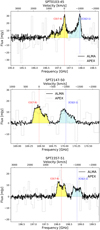 |
Fig. 1. Integrated spectra of SPT0103−45 (top panel), SPT2147−50 (middle panel) and SPT2357−51 (lower panel). The black solid line is the spectrum extracted from the ALMA observations (see Sect. 2.3). The light grey line is the APEX/SEPIA spectrum (see Sect. 2.1). Red and blue vertical dashed lines indicate the position of CO(7−6) and [CI](2−1) lines, respectively, at the reference redshift of the source. The yellow and cyan shaded areas show the integration windows used to compute integrated fluxes of the CO(7−6) and [CI](2−1) lines, respectively (see Sect. 4.3). The zero-velocity corresponds to the observed frequency of CO(7−6) line for each of the sources. |
Our third source, SPT2147−50, was not detected with APEX despite the second data reduction, showing a weak signal for CO(7−6) (Fig. 1). However, SPT2147−50 is a part of the Targeting Extremely Magnified Panchromatic Lensed Arcs and Their Extended Star formation (TEMPLATES) James Webb Space Telescope (JWST) Early Release Science programme3. The source was thus observed with ALMA in CO(7−6), [CI](2−1), and the dust continuum to aid in the interpretation of the upcoming JWST data (PI: Vieira, 2018.1.01060.S).
Figure 2 shows the line luminosity of [CI](2−1) and CO(7−6) against the IR luminosity. We compare our sources with the sample compilation presented in Valentino et al. (2020). Our sources are at the bright end of the SMG cloud. Our final sample thus consists of three sources: SPT0103−45, SPT2147−50, and SPT2357−51. Our sources are presented in Table 2.
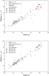 |
Fig. 2. Line luminosity of [CI](2−1) (top-panel) and CO(7−6) (bottom-panel) vs. infrared luminosity. All the luminosities in this plot are not corrected for magnification. Our sources (filled squares) are compared with the SMGs (stars), main-sequence at z ∼ 1 (diamonds), local galaxies (dots), AGN and QSO (hexagons) from the compilation of Valentino et al. (2020). |
Our sample.
2.3. ALMA observations
All our targets were observed with the ALMA 12-m array using the Band-5 receivers and in the C43-5 configuration (shortest baseline: 15 m; longest baseline: 1400 m). The requested angular resolution was 0.3″ for SPT0103−45 and SPT2357−51, and 0.4″ for SPT2147−50. This was the best possible angular resolution allowed in Band 5 during Cycle 5 and allows us to resolve the sources over several synthesised beams.
To observe CO(7−6) and [CI](2−1), two spectral windows with 1.875 GHz bandwidth and 7.813 MHz resolution (corresponding to 11−13 km s−1 velocity resolution) were used4. For each source, we also placed two other spectral windows in the other sideband to measure the continuum. The same spectral resolution was used for SPT0103−45 and SPT2357−51, while 31.25 MHz was used for SPT2147−50.
To characterise the dynamics of these systems, we need to securely constrain the position of the peak of at least one line in each synthesised beam. For SPT0103−45 and SPT2357−51, we chose the target sensitivity to obtain a 10σ detection when integrated over the full line width. We estimated the signal and the line width from the APEX spectra (Sect. 2.1) and divided the flux into the number of synthesised beams covered by the source from the previous 870 μm continuum imaging and lens model (Spilker et al. 2016). We derived a target sensitivity of 80 μJy beam−1 in a 320 km s−1 channel for SPT0103−45 and 67 μJy beam−1 in a 510 km s−1 channel for SPT2357−51. For SPT2147−50, the sensitivity was estimated by rescaling the observed continuum profile to the estimated CO and [CI] flux, aiming for a 6σ detection over 1/3 of the line width at the peak of the detection, which is equivalent to 10.4σ over the full line width. This corresponds to 100 μJy beam−1 in a bandwidth of 100 km s−1 (1/3 of the line width) or 58 μJy beam−1 in a bandwidth of 300 km s−1. The target sensitivities for the three sources are thus rather similar in the end. The details of the observations are presented in Table 3.
Observational details.
3. Data processing
3.1. Calibration
Initial calibrations were done by the observatory using the standard ALMA pipeline based on the Common Astronomy Software Applications (CASA) (McMullin et al. 2007). Since our sources are bright, we attempted to self-calibrate the phase solutions. However, many long baselines were poorly fit and were thus flagged. The beam size was consequently degraded without a significant gain in sensitivity, so we discarded the self-calibration.
3.2. Continuum imaging
To image the data, we used the CLEAN routine in CASA. The data were imaged using a pixel size of 0.04″ in order to finely sample the synthesised beam (∼10 pixels per beam). A Briggs weighting (Briggs 1995) of the visibilities, with a robust parameter of 0.5 was chosen to give the best compromise between S/N and angular resolution.
To measure the continuum, we combine the two spectral windows in the line-free sideband and the channels without line contamination in the sideband where CO(7−6) and [CI](2−1) are located. These channels are identified using a first preliminary line imaging (see Sect. 3.3). The continuum images are then generated using a multi-frequency synthesis (MFS) method (Conway et al. 1990). A first imaging is made to estimate the noise level (hereafter σnoise). We then perform a second imaging using 3σnoise from the previous imaging as the Clean threshold. The first row of Fig. 3 shows the resulting continuum maps of our sources.
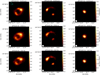 |
Fig. 3. Continuum and moment-0 maps of our sample. First row: continuum maps of (from left to right) SPT0103−45, SPT2147−50, and SPT2357−51 (see Sect. 3.2). The synthesised beam is represented as the white ellipse on the bottom left of every map. Second row: is the integrated [CI](2−1) intensity maps. Third row: is the integrated CO(7−6) intensity maps of our sources (see Sect. 4.3). |
3.3. Line imaging
Using similar parameters as for the continuum, we first image the spectral window(s) covering CO(7−6) and [CI](2−1). We then subtract the continuum directly in the uv plane using the uvcontsub CASA task. The channels that are line-free in our initial image cube are used to fit and subtract the continuum. We assume a constant continuum level (as a function of the frequency) for SPT2357−51 and a first-order polynomial for the two other sources as the first-order polynomial gave a better fit of the continuum. We then re-imaged the data to obtain a continuum-subtracted line cube. No rebinning from the native ∼12 km s−1 spectral resolution was used in the process, since the S/N per channel is sufficiently high.
3.4. Imaging performance
For the continuum, the synthesised beam major axis size is between 0.43″ and 0.48″, while the minor axis size is between 0.35″ and 0.41″. The axis ratio varies from 1.17 to 1.21.
Concerning the line cubes, for SPT0103−45 and SPT2147−50 the synthesised beam is slightly larger than for the continuum, with the major axis ranging from 0.47″ to 0.48″ and the minor axis ranging from 0.39″ to 0.42″. This is because the spectral lines are located in the lower sideband of the frequency coverage. Conversely for SPT2357−51, the continuum has a coarser resolution because the lines are in the upper sideband, so the continuum-only data is at a lower average frequency. The beam axis ratio varies from 1.12 to 1.22. Overall, all three sources have similar, nearly circular beams. We estimate the noise level at the phase centre by computing the standard deviation in the non-primary beam corrected map after masking the source. The average continuum sensitivity varies from 13 to 25 μJy beam−1. The same procedure is used channel by channel for the line cubes. The mean sensitivity per channel and the range of sensitivities per channel for every source are summarised in Table 4.
Imaging performance.
4. Integrated spectra and source morphologies
4.1. Continuum morphology
The dust continuum images are shown in the upper panels of Fig. 3. SPT0103−45 is ring-shaped, which is characteristic of strongly lensed sources (Spilker et al. 2016). The brightest region is located in the north-west (henceforth, the gem) and another bright region can be seen in the south-east. They correspond to two counter-images of the same region of the source (see Sect. 6).
SPT2147−50 exhibits an extended arc in the north-east and a compact counter-image in the south-west (see Sect. 6). The northeast arc is brighter in its most eastern part and there is a small gap with no detected continuum at the most northern part of the arc.
SPT2357−51 is also gravitationally lensed and has a very compact continuum emission compared to the other sources. The compact emission is due to the small Einstein radius of the foreground lens galaxy (θE ∼ 0.2″, Spilker et al. 2016). The resolved structure of SPT2357−51 is difficult to see visually in our default continuum image using all the line-free channels and a Briggs weighting with a robustness parameter of 0.5. In order to demonstrate the lensing geometry of this source more clearly, we re-imaged the continuum selecting only visibilities on baselines > 200 kλ, shown in Fig. A.1. We note that this image is for demonstration purposes only, as our lens modelling procedure (Sect. 6.2) fits directly to the interferometric visibilities and is not influenced by choices in imaging parameters.
The total continuum flux density is estimated from these maps by integrating the flux in an elliptical region encompassing the entire source. The continuum fluxes are tabulated in Table 1. To estimate the uncertainties of these fluxes, we select a polygonal region near the source and measure the noise rms in this region. We then re-scale this noise by the factor of  , where N is the number of synthesised beams in the elliptical region where the source flux is estimated. We combine this statistical uncertainty with the estimated 10% absolute flux calibration typical of ALMA data.
4.2. Integrated spectra
We extract the integrated spectra from the line cubes after manually selecting the emission region. This process was repeated multiple times to ensure the robustness of the method. Figure 1 shows the integrated spectra of all our sources. There is a clear detection, S/N > 14, for both the CO(7−6) and [CI](2−1) lines in all sources.
The line profiles of SPT0103−45 show a well-defined peak along with a redshifted tail in both CO and [CI] (Fig. 1, top panel). These tails extend to about +1000 km s−1. The uni-directionality of the high-velocity tail is interesting and will be further explored in Sect. 5.1. The [CI](2−1) tail is slightly blended with the CO(7−6) peak emission and cannot be well isolated. We assessed the impact of this line blending by fitting the spectrum of SPT0103−45 with the sum of three Gaussian profiles each, for CO and [CI], fixing the centre velocity relative to each line’s systemic velocity and the width of each pair of components (i.e. with a total of 12 free parameters to fit both lines simultaneously: three centre velocities, three Gaussian line widths and six amplitudes). We find that accounting for the line blending increases the [CI]/CO line ratio by ∼5% compared to the simple division illustrated in Fig. 1. We increase the uncertainty on the measured line ratio by this amount, added in quadrature to the statistical uncertainty from the noise in the data. The deblending procedure and results are further demonstrated in Appendix B.
In SPT2147−50, both the lines are broad (FWHM ∼ 550 km s−1) and asymmetric, with the redshifted side brighter than the blueshifted side of the spectra (see Fig. 1, middle panel).
For SPT2357−51, the line profiles show double peaks in both lines (see Fig. 1, bottom panel). The blueshifted peak is slightly brighter (∼2 mJy) than the redshifted peak. The nature of this double peak feature will be further explored in the Sect. 5.3.
In Fig. 1, we compare the ALMA spectral profile with the APEX/SEPIA observations. We also re-estimate the APEX line fluxes using a broader integration window corresponding to the entire width of the line seen by ALMA (blue and yellow shaded regions of Fig. 1). The results are tabulated in Table 1. While the shape of the APEX and ALMA spectra generally agree, there are differences up to 2σ in the integrated line fluxes. It is unlikely to be an interferometric effect (e.g. filtered-out large-scale emission) since the largest difference is found for SPT2357−51, the most compact source of our sample. It is more likely that the APEX spectrum is simply of lower quality than the ALMA spectra.
4.3. Line morphologies
We construct integrated intensity (i.e. moment-0) maps of the [CI](2−1) and CO(7−6) lines by summing the flux of every channel covering the line using the CASA immoments task. We define a frequency range for each line as the integration window to compute the integrated intensity from the continuum-subtracted datacubes. The integration windows are shown in Fig. 1, with CO(7−6) in yellow and [CI](2−1) in blue. For SPT0103−45, the most redshifted CO(7−6) emission is blended with the most blueshifted [CI](2−1) emission, as noted above. We thus use a narrower range to integrate the [CI](2−1) emission in order to avoid the contamination of CO(7−6) emission, but note that the line blending introduces some unavoidable uncertainty into the moment maps.
The moment-0 maps for the [CI](2−1) and CO(7−6) lines are shown in the second and third rows of Fig. 3 respectively. The line emission is more extended than the continuum emission for all sources. The compactness of the dust continuum with respect to spectral lines that trace cold gas is very common in DSFGs (e.g. Spilker et al. 2015; Calistro Rivera et al. 2018; Dong et al. 2019; Apostolovski et al. 2019).
We estimate the line intensities of the sources by selecting the region encompassing the source manually and obtaining the intensities in this region. The uncertainties are estimated similarly to the continuum emission (Sect. 3.2). The intensities are tabulated in Table 1.
5. Image-plane kinematics
5.1. SPT0103–45
The two most intriguing features in this source are the high-velocity redshifted tail visible in both lines (see Fig. 1, top panel) and the presence of a particularly bright continuum feature, which we call the ‘gem’.
Such high-velocity tails are often seen as signatures of molecular outflows driven by AGNs (e.g. Maiolino et al. 2012; Cicone et al. 2014; Florez et al. 2021; Pantoni et al. 2021) and/or supernovae (Ginolfi et al. 2020; Spilker et al. 2020a,b). However, we see high-velocity tails only in one direction which makes it unlikely to be a signature of an outflow. We further explore other explanations such as magnification effects that could result in distorting the line profiles (see Sect. 6.7).
To try to understand the nature of SPT0103−45, we extract the spectra at the pixel where the continuum flux density is maximal, i.e. at the position of the gem. Figure 4 shows the spectrum at the position of the gem, clearly showing very broad and blended lines. The high-velocity tail is almost as bright as the peak of the emission near the systemic velocity. We also reconstruct the integrated intensity map of the high-velocity emission of CO(7−6) using the integration range shown in yellow in the centre panel of Fig. 4. The 3, 5, and 10σ contours of the continuum are also plotted on the high-velocity intensity map shown in the bottom-right panel of Fig. 4. This reveals a small spatial offset between the high-velocity regions and the brightest continuum region.
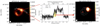 |
Fig. 4. Properties of the ‘gem’ in SPT0103−45. Left panel: is the continuum map as described in Sect. 3.2. The white line shows the direction along with the slice for the PV diagram is extracted (Fig. 6). The spectrum shown in the centre panel is extracted at the coordinates of the gem (Sect. 3.3). The frequency range represented by the yellow region is used to compute the integrated intensity of the high-velocity emission, represented in the right panel. The white contours are the 5, 10 and 15σ contours of the continuum emission. |
We then build the velocity map of the source. To avoid artifacts caused by magnification or high-velocity components, we mapped the peak velocity of each line for each line of sight instead of a moment-1 map. To do that, we extract the spectrum at each pixel and fit a linear spline to reduce the impact of the noise. We then identify the peak of emission and the velocity corresponding to it. We search for the lines in the 197.5−198.1 GHz range (727.1 to −257.5 km s−1) for [CI](2−1) and 196.5−197.38 GHz (866.2 to −45.6 km s−1) for CO(7−6). These intervals were chosen to avoid cross-contamination between the two lines in the region, where low-velocity CO(7−6) and high-velocity [CI](2−1) could overlap. To ensure that this peak is real, we require that the maximal flux determined by the spline fit should be above 3σ.
In Fig. 5, we show maps of the mean velocity of each line (i.e. moment-1 maps). To allow a better visualisation of the geometry of the source, the 3, 5, and 10σ contours of the continuum are plotted on the velocity maps. For both lines, we observe a very similar velocity gradient from east to west. However, the high-velocity regions corresponding to the redshifted tail are all located west of the gem.
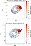 |
Fig. 5. Pixel-wise peak velocity decomposition of SPT0103−45. Top row: velocity map of the [CI](2−1) line and bottom row: CO(7−6) line. The 5, 10, and 15σ contours of the continuum emission are plotted on all velocity maps. The construction of these maps is described in Sect. 5.1. |
To further analyse the kinematics of the source, we construct position-velocity (PV) diagrams along the bright arc passing through the gem. The slice is indicated as the white line in the left panel of Fig. 4. The PV diagram is shown in Fig. 6. The zero velocity corresponds to the observed frequency of the CO(7−6) line. The PV diagrams of both lines are similar in profile. From a position 0 to 1.5 arcsec, the velocity is almost flat followed by a quick increase between 1.5 and 2 arcsec, and finally a second plateau around ∼800 km s−1. The second plateau is much fainter, which could be due to differential magnification (see Sect. 6.4).
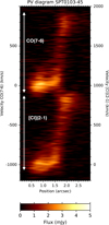 |
Fig. 6. Position-velocity diagram of SPT0103−45. The axis used to make this diagram is shown in the first panel of Fig. 4. The velocity axis on the left y-axis has the zero-velocity of the CO(7−6) observed frequency and the right y-axis has the zero-velocity centred at the [CI](2−1) observed frequency. |
5.2. SPT2147–50
The [CI](2−1) and CO(7−6) lines of SPT2147−50 are broad and asymmetric with more flux on the redshifted side (see Fig. 1). To understand the origin of the asymmetric and broad lines, we construct a pixel-wise velocity map.
Since the lines are not always symmetric even in a given pixel, we locate the line peak velocity using a similar approach as for SPT0103−45 (see Sect. 5.1). As only one single peak per line can be found along any given line of sight, we define a single velocity range from −400 to +400 km s−1 to search for the peak.
These peak velocities are then used to construct the velocity maps seen in Fig. 7. We also plotted the 3, 5, and 10σ contours of the continuum emission to better visualise the geometry of the source. The velocity maps measured independently for each line are strikingly similar. The peak velocity varies from −300 to 150 km s−1. We observe a smooth velocity gradient from east to west in the northern arc and the opposite in the south arc, as expected for a gravitationally lensed arc and counter-image (see further discussions in Sect. 6.5).
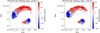 |
Fig. 7. Pixel-wise peak velocity decomposition of SPT2147−50. The velocity maps of [CI](2−1) (left) and CO(7−6) (right) are shown. The 3, 5, and 10σ contours of the continuum are overplotted on the velocity maps. The construction of these maps are described in Sect. 5.2 |
5.3. SPT2357–51
The line profile of both lines has a doubly peaked profile (see Fig. 1). A similar profile was observed for the [CII] line of SPT0346−52, which has been identified as a major merger (Litke et al. 2019). To assess whether SPT2357−51 may also be a merging system, we first examine the position-velocity diagram extracted along the right ascension axis (Fig. 8), chosen to maximise the spatial separation between the two components. It shows two clearly separated components: a western component at blueshifted velocities (henceforth, the blue component) and an eastern component at redshifted velocities (henceforth, the red component). Their peaks of emission are separated spatially by about ∼1″ and spectrally by ∼400 km s−1.
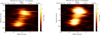 |
Fig. 8. The position-velocity diagram of the [CI](2−1) and CO(7−6) lines of SPT2357−51. The slice was taken along the RA axis. |
To characterise both components seen in the position-velocity diagram, we performed a pixel-wise decomposition of the spectra into two Gaussian components for each line.
We extract the continuum-subtracted spectrum for each pixel and fit it with four Gaussian profiles (two for each line). To ensure a physical and meaningful result, we applied several constraints. The amplitude is forced to be positive, since we do not expect to see CO(7−6) or [CI](2−1) in absorption in such a system. The line width is allowed to vary from 0 to 250 km s−1 to avoid unphysically broad components. Finally, we define a velocity range associated with each component in order to avoid overfitting one component with two Gaussians if one component is very faint. The bounds for the central velocity of the peaks were defined from the velocity separation seen in the position-velocity diagram. The red component is fitted in a velocity range between 0 and +250 km s−1 and the blue component between −150 and −300 km s−1 for both [CI](2−1) and CO(7−6) lines.
To derive uncertainties on the amplitude, width and position of our Gaussians, we measure the noise in each channel and take it into account with the fitting tool (curvefit from the scipy package). In the rest of the analysis, we only consider results for which the significance of the amplitude is higher than 3σ. The residuals are below 2.5σ for every fit.
Figure 9 shows the velocity map for each of the components of the [CI](2−1) and CO(7−6) lines along with the 3, 5, and 10σ contours from the continuum map. The velocity gradients obtained for CO(7−6) and [CI](2−1) are remarkably similar. The blue component shows a smooth velocity gradient suggestive of rotation. The velocity structure of the red component is less clear, showing essentially no coherent structure.
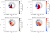 |
Fig. 9. Decomposition of the CO(7−6) and [CI](2−1) lines in SPT2357−51. The central velocity of each component from the Gaussian fitting is shown above. The fitting procedure is described in Sect. 5.3. The 3, 5, and 10σ contours from the continuum map are also plotted on the maps. We see a smooth velocity gradient for the blue component, but no discernible pattern in the red component. |
The continuum is centred on the red component while the blue component is an offset from the peak of the dust continuum. Since these two components have similar apparent line luminosities, this could indicate that the red component has a larger dust emission and/or stronger obscured star formation. This could originate from different gas metallicities or temperatures between the two components. This difference of ISM properties between the two velocity components is a clue that this object could be a merger between two galaxies. It is unlikely that differential magnification could cause the low dust emission of the blue component. Lensing is a purely geometric effect, so any given individual region must have the same magnification for the lines and the continuum. Further discussion on the geometry of this source based on lens modelling will be done in Sect. 13.
6. Lens modelling
To understand the source-plane morphology and derive the intrinsic properties of the galaxies in our sample, we perform lens modelling of both the continuum and CO/[CI] line emission. Modelling spectral velocity channels separately allows us to characterise the dynamics of these systems and quantify potential differential magnification effects both across the line profiles and in comparison to the continuum (Serjeant 2012; Hezaveh et al. 2012; Paraficz et al. 2018; Dong et al. 2019).
6.1. Method
We use the lens modelling code visilens from Spilker et al. (2016). It directly models Fourier-plane interferometric visibilities instead of the inverted image plane to limit the biases caused by correlated noise generated by the imaging algorithm. This also helps us better account for the antenna delay and the mismatched absolute flux calibration that could arise due to combining multiple observations taken on different days, which is the case for SPT2147−50. The angular resolution of our data does not allow us to make a reliable pixelated reconstruction of the source-plane.
Our model describes the foreground lens with one singular isothermal ellipsoid (SIE) profile. The profile is parametrised by the following free parameters: the position of the lens relative to the phase centre (xL, yL), the angular Einstein radius θE, L, the ellipticity eL and the position angle of the major axis ϕL. The background sources are modelled with Sérsic (1968) and/or Gaussian profiles, for both the continuum emission and each spectral channel. The position of the source (xS, yS) is defined relative to the lens position. The other parameters are total flux density (S), effective half-light major axis (aS), axis ratio (bS/aS), Sérsic index (nS), and position angle (ϕS). We note that models with substantially more freedom in the source morphology, such as a pixellated source plane (e.g. Dye et al. 2015; Hezaveh et al. 2016) are not warranted for our moderate-resolution data. Visilens uses a Monte Carlo Markov chain (MCMC) fitting procedure to sample the parameter space (Spilker et al. 2016). The best-fit parameters are then determined after the chains converge. We finally produce model dirty images, high-resolution models and source plane models from the best-fit model (see Fig. 10).
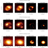 |
Fig. 10. Modelling the continuum emission of our sources. SPT0103−45 is in the first row, SPT2147−50 in the second row and SPT2357−51 in the third row. For every source, the first panel (from the left) is the dirty image of the continuum, the second is the dirty image produced by best-fit model, third is a ‘high-resolution’ image-plane model, i.e. not sampled by the uv coverage of the data and the fourth panel is the best-fit model in the source plane. In the third and fourth panels, the lensing caustics are shown in white. |
6.2. Continuum modelling
To perform the lens modelling of the continuum, we select only the data from the line-free spectral windows. We then average the two orthogonal polarisations. We choose a first estimate of the lens and source parameters using the previous modelling performed on low-resolution data by Spilker et al. (2016) and define loose reasonable priors (e.g. positive fluxes, 0 < nS < 4). We use a single component for the source profile of SPT2147−50 and SPT2357−51 but two components for SPT0103−45, as the model gave us lower residuals. We use 50 chains of 10 000 usable steps and 1000 burn-in steps to run the MCMC chains and verify the chains converged. We also check that the marginalised parameter distributions do not return a high probability for values close from the prior limits. The best-fit lens parameters for all our sources are given in Table C.1. These parameters are in agreement with the best-fit lens parameters from Spilker et al. (2016).
6.3. Line modelling
In order to model the line emission of [CI](2−1) and CO(7−6), we use the continuum-free visibilities described in Sect. 3.3. We divide the lines into frequency bins with widths that ensure that the line emission is detected at a peak S/N ≳ 8 in each channel. For SPT2147−50 and SPT2357−51, we use 50 MHz bins (∼80 km s−1). For SPT0103−45, we use 100 MHz bins (∼150 km s−1) for the redshifted tail where the emission is faint and narrower bins of 40 MHz width (∼50 km s−1) at the line peak where the S/N is high.
Since the S/N of the continuum is much higher than any of the lines, we simply fix the parameters of the lensing potential for all velocity channels of each source to those found in the continuum modelling. The source parameter starting values are also derived from the continuum analysis, but these parameters are allowed to vary. We use 40 chains of 10 000 usable steps and 1000 burn-in steps for each of the runs. We verify that the chains converged for every run. The best-fit parameters for the line modelling of SPT0103−45, SPT2147−50 and SPT2357−51 are listed in Tables C.2–C.4 respectively.
6.4. SPT0103–45
For the continuum of SPT0103−45, a single source component was insufficient to properly fit the visibilities, thus we use two Sérsic components to model the source. The best-fit model converged to a solution with an extended component (nS = 0.994 ± 0.011, see Table C.2) and a second very compact component (reff = 0.055 ± 0.002 arcsec). The maximum continuum residuals were ∼8.3σ, approximately 4% of the peak S/N in the data. This illustrates how difficult it is to model our very high S/N continuum data even with two components and suggests that a future approach with more freedom in the source plane (e.g. pixellated modelling) could be more successful. The dirty image of the data and best-fit model are shown in Fig. 10 (top-right panel) together with a high-resolution model (neglecting the Fourier-plane sampling) and the source-plane emission. The best-fit parameters of both the components are given in Table C.2. The intrinsic flux ratio of these two components is about 17, with the extended component being brighter. The nature of this second component is unclear and we cannot conclude based on our data if it is a clump in the disk, a compact neighbour, or even an artifact of the model to mimic an asymmetry of the disk in the source plane.
To model the CO(7−6) and [CI](2−1) line data in each velocity bin, a single Sérsic source was sufficient. We start our MCMC chains from the best-fit parameters of the extended continuum component. The highest residuals are < 5σ, except for one velocity bin (centred at ∼136 km s−1) for which the maximum residual was ∼7σ. In Figs. E.1 and E.2, we compare the best-fit model and the observed data for the [CI](2−1) line and the CO(7−6) line, respectively.
In Fig. 11, we plot the best-fit source position and size for every velocity bin for each of the lines. We can see a smooth velocity gradient across the source, consistent for both the lines. Emission at blueshifted velocities is close to the inner diamond caustic, while the most redshifted emission is near the outer caustic. The results thus favour a scenario in which SPT0103−45 is a rotating disk.
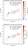 |
Fig. 11. Best-fit source positions of the channelised models of [CI](2−1) (top) and CO(7−6) (bottom) in SPT0103−45. The velocity scaled is the central velocity of each of the bins. The black square and cross, represent the positions of the extended and compact component from the continuum model, respectively. The ellipses represent the half-light ellipses of each of the model. The lensing caustics are shown in grey. |
6.5. SPT2147–50
In the case of SPT2147−50, the source was observed on three different days (see, Table 3). At each step of the MCMC code, we separately compute the likelihood of the data corresponding to each day and then combined them. To take into consideration the different atmospheric conditions and the small calibration offsets that could occur in these observations, we introduce two multiplicative amplitude re-scaling as free parameters for the latter two observations. In simple terms, these parameters account for the fact that SPT2147−50 is detected with S/N ≫ 20 while the absolute flux scale of ALMA data is quoted by the observatory to be accurate at the ∼5 − 10% level.
For both the continuum and the line models, we use a single component with a Sérsic profile. This relatively simple model is sufficient to fit our source. The continuum residuals are lower than 1.5σ and the residuals for the line modelling are always below 4σ in any velocity channel. In Fig. 10 (middle row), we show the continuum dirty image and the modelled dirty images together with the high-resolution model and the source plane model. The comparison between the model and the dirty image in each velocity channel is presented in Figs. E.3 and E.4.
The best-fit value of the Sérsic index for the continuum is 1.36 ± 0.05 (see Table C.3). This index, close to 1, is compatible with the hypothesis that the object is a rotating disk (see also Sect. 5.2). The best-fit parameters for the line and continuum modelling are presented in Table C.3. The source plane model (see Fig. 10) shows that part of this disk-like profile is near the inner caustic. Significant differential magnification effects (see Sect. 6.7) can thus be expected.
In Fig. 12, we present the source-plane reconstruction of the CO and [CI] line emission. We see a clear shift of the source position with velocity. The continuum centre of emission (in black) coincides with velocities nearest the systemic velocity. The eastern region is blue shifted, while the western region near the caustic is redshifted. The gradient is similar for both lines. Overall, the centre of emission regions at the various velocities are well aligned. This provides an additional evidence that the source could a rotating disk.
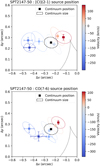 |
Fig. 12. Best-fit source position of SPT2147−50 for both [CI](2−1) (top) and CO(7−6) (bottom). The velocity scale is the central velocity of each of the bins. The black square represents the position of the continuum. The ellipses represent the half-light ellipses of each model. The lensing caustics are shown in grey. |
6.6. SPT2357−51
For SPT2357−51, the decomposition of the spectrum along the various line of sight was suggestive of a two-component system (see Sect. 5.3). However, a single source-plane Gaussian component was sufficient to model the data and gave low residuals (1.72σ), likely due to the low spatial resolution of our data and the compact lensing geometry. The best-fit parameters of the continuum lens model are presented in Table C.4. In Fig. 10 (lower panels), we present the results of our best-fit continuum model.
The same source model is used in each velocity bin. The largest residuals for each of these bins are < 5σ. In Fig. 13, we plot the position of the source for different velocities. The geometry of this source is more disturbed than the two other sources. While, there is a velocity gradient for the velocities corresponding to the blue component, the geometry associated to the red component (> 0 km s−1) is much more disturbed. The kinematics from our source-plane reconstruction are only marginally consistent with the expectation for rotation, though it is hard to constrain the emission region for the red component because the signal is emitted very close to caustics. Similar to the image-plane kinematic analysis (Sect. 5.3), we also find that the continuum is offset from the main region of gas emission. Our source-plane reconstruction thus favours the scenario of a disturbed kinematics possibly linked to a merger.
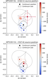 |
Fig. 13. Best-fit source position of SPT2357−51 for both [CI](2−1) (top) and CO(7−6) (bottom). The velocity scale is the central velocity of each bin. The black square represents the position of the continuum. The ellipses represent the half-light ellipses of each model. The lensing caustics are shown in grey. |
6.7. Differential magnification
From the results of the lens modelling for our sources, we find differences in the magnification between the continuum and the line emission as well as across the CO and [CI] line profiles. Figure 14 shows the magnification as a function of velocity for both CO(7−6) and the [CI](2−1) along with the continuum magnification (horizontal blue dotted line). We note that the systemic redshifts of the sources were measured from the apparent spectra (not the intrinsic spectra). We also plot the CO(7−6) and [CI](2−1) observed spectra along with the magnifications to differentiate the intrinsic features from those arising due to magnification effects.
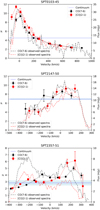 |
Fig. 14. The variation of the magnification as a function of velocity for the [CI](2−1) line (red filled squares) and the CO(7−6) line (black filled circles). The blue line is the continuum magnification and the blue shaded region indicates the 68% confidence interval. Top panel: results for SPT0104−45. Middle panel: for SPT2147-50 and bottom panel: for SPT2357−51. We also overplot the observed spectra using a dashed-line, red for [CI](2−1) and black for CO(7−6). |
For SPT0103−45, the agreement between the observed line profile (dashed lines) and the magnification profile (points and dotted lines) in Fig. 14, top panel, demonstrate that the velocity-dependent magnification is largely responsible for the line shape in this object.
For both lines, the magnification of SPT2147−50 increases towards redshifted velocities. The line profile of SPT2147−50 is similar to SPT0103−45 with respect to the magnification versus velocity, except that in this case the redshifted side is more magnified. The asymmetry of the integrated line profile is again likely due to differential magnification.
The red component of SPT2357−51, which was brighter in the continuum (see Sect. 5.3 and Fig. 9), is more magnified than the blue component. Since they have similar apparent line fluxes, the red component is thus intrinsically fainter.
For each source, we calculated the effective magnification (μeff) of each line. It is computed as the ratio between the sum of the apparent flux in all velocity bins and the sum of the intrinsic fluxes in the same bins:
 (1)
(1)
where μ is the magnification in each of the bins, Δυ is the width of the bin, and Sν is the intrinsic flux density. In our lens model, the magnification and the intrinsic flux are correlated because the total apparent flux density is very well constrained by the data. We thus do not estimate uncertainties on μeff by combining the marginalised uncertainties on the input quantities. We instead calculate the effective magnification for all MCMC steps and compute the median and the standard deviation of the obtained values. The effective magnifications are tabulated in Table 6.
For SPT2147−50 and SPT2357−51, the CO(7−6), [CI](2−1), and the continuum magnifications are similar with variations < 15%. There is thus no evidence for strong differential magnification on integrated flux measurements. For SPT0103−45, we find a larger difference between the [CI](2−1) and continuum magnification (∼24%), and between the CO(7−6) and the continuum (∼16%). Traditionally, luminosity ratios are used to mitigate magnification effects in lensed sources. This assumes implicitly that the luminosity of all the lines and the continuum are magnified in the same way. Our analysis suggests that it is a reasonable assumption in general, but can introduce small biases depending on the lensing configuration of the individual sources. In contrast, our results show that spectral line profiles can be significantly distorted by differential magnification. Differential magnification effects are more severe across the line profiles than between the dust continuum and molecular gas tracers.
7. Resolved line and continuum ratios
7.1. Ratio maps
Analysing the resolved line and continuum ratios can help to understand the ISM properties of our sources. The bolometric infrared luminosity between 8 and 1000 μm (LIR) is a well-known tracer of the SFR of galaxies (Kennicutt 1998). The [CI](2−1) line can be used as a tracer of the total molecular gas (e.g. Papadopoulos et al. 2004) and the high-J CO lines are a tracer of the dense molecular gas (e.g. Weiß et al. 2007). Combining these three tracers, we can map both the resolved star formation and gas properties in our objects. We continue our ratio analysis in the image plane. This avoids the introduction of any artifacts in the line ratio due to our parameterised models for the source-plane emission. As gravitational lensing conserves surface brightness, an image-plane analysis is also equivalent to the same analysis in the source plane, with the caveat that multiply imaged regions of the source plane appear multiple times in the image plane.
To compute the continuum to line ratios accurately and avoid resolution effects, our continuum and line maps must have comparable resolutions. In Table 4, we notice that the continuum has a slightly smaller synthesised beam size than the lines. This is a result of the frequency coverage of our data, since most data used for the continuum imaging comes from the other sideband, 12 GHz higher in frequency, that samples the uv plane at slightly higher spatial frequencies. Hence, we produce another set of continuum maps using only the line-free continuum channels from the same sideband as the lines to more closely match the synthesised beam size between lines and continuum.
To obtain physically meaningful ratios, we convert both continuum and line fluxes in each beam into apparent luminosities. For the continuum maps, we use the following conversion to derive the apparent infrared luminosity per beam (μLIR(beam)):
 (2)
(2)
where Sν, (beam) is the continuum flux density per beam measured in any pixel of the continuum map, Sν(total) is the total continuum flux density integrated over the entire source and μ LIR is the total apparent infrared luminosity determined by Reuter et al. (2020) from Herschel and ground-based photometry.
This conversion implicitly assumes that the shape of the spectral energy distribution (SED) is the same everywhere in the galaxy. This is an approximation. Using simulations, Cochrane et al. (2019) estimated the dust temperature (Tdust) gradient in star-forming galaxies (γ in Tdust = Tcenter rγ5, where r is the distance from the centre in kpc). They found a range of γ between −0.3 and −0.05. For the smallest γ and the largest source (SPT0103−45), we obtain a temperature variation by a factor of 1.4 between the centre and the half-light radius. Assuming a simple L ∝ T4 scaling, this corresponds to a factor of 3.5 in luminosity at constant flux. For γ = −0.05, the effect is much smaller, with only a 24% luminosity difference.
For the line flux maps, we use the conversion formula from Solomon et al. (1992)
 (3)
(3)
where Sline(beam)Δυ is the value obtained from the line flux maps derived in Sect. 4.3, in the units of Jy km s−1 beam−1, DL is the luminosity distance of the source in Mpc and νobs is the observed line frequency in GHz. The total line luminosities and IR luminosity corrected for magnification for all our sources are tabulated in Table 5. We use the effective magnifications of the continuum or the associated line computed in Sect. 6.7 and listed in Table 6. The uncertainties on the line luminosity ratio of SPT0103−45 are the combined uncertainties derived from the moment map luminosities and the luminosities estimated by deblending the lines (see Appendix B).
Line and infrared luminosities of the sources.
Differential magnification.
We then create L[CI](2−1)/LIR and L[CI](2−1)/LCO(7−6) ratio maps, shown in Fig. 15 using a 3σ threshold on the IR and line luminosities. SPT0103−45 has a lower [CI]/continuum ratio and marginally lower [CI]/CO ratio at the position of the gem. In SPT2147−50, the northeast part of the main arc and its southern counter-image show a lower [CI]/continuum than the western part of the arc, while no obvious features are seen in the [CI]/CO ratio map.
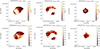 |
Fig. 15. The [CI]/continuum ratio maps are in the upper panels and the [CI]/CO line ratio maps are in the lower panels for SPT0103−45, SPT2147−50 and SPT2357−51, from left to right. The 5, 10, and 15σ contours of the continuum are plotted on the ratio maps (in magenta). The computation of these ratios are described in Sect. 7.1. The synthesised beam is represented as the black ellipse in the bottom left of every map. |
The [CI]/continuum ratio of SPT2357−51 exhibits a higher value in the centre than on the outskirts. This may be counter-intuitive, since galaxy sizes measured from gas tracers are usually larger than from the continuum (Spilker et al. 2015; Dong et al. 2019; Apostolovski et al. 2019; Fujimoto et al. 2020). This central region could correspond to the overlap of the two components of this candidate merger system (see Sect. 5.3). In this interacting region, the continuum luminosity could possibly be underestimated if the dust is warmer in the core of this object. We again see no clear pattern in the [CI]/CO ratio map. For this source, higher-resolution data would be necessary to make stronger conclusions, given the compact lensing configuration of this source.
We next compare the luminosity ratios of our sources with other lensed SMGs. Andreani et al. (2018) found LCO(7 − 6)/L[CI](2 − 1) ratios of 2.5 and 4.06 for their sample. Yang et al. (2017) found that the line ratio vary from 0.8 to 3.0 in their sample of Herschel-selected SMGs. These ratios are typically higher than we measure in our sources, i.e. 0.93 ± 0.02 for SPT0103−45, 1.2 ± 0.1 for SPT2147−50 and 1.6 ± 0.1 for SPT2357−51. Our ratios are consistent with the ratios seen in local galaxies by Kamenetzky et al. (2014, from 0.4 to 2) and close to the value for the Milky Way centre (0.91) measured by Fixsen et al. (1999). Our systems thus have less extreme line ratios than the Herschel-selected lensed galaxies of Andreani et al. (2018). Those authors claim that the LCO(7 − 6)/L[CI](2−1) ratio can be indicative of whether a system is disk-dominated (line ratio ∼1) or merger-driven (up to ∼10). According to the dynamics and the lensing reconstruction of our sources performed in Sects. 5, 6 and 8, SPT0103−45 and SPT2147−50 seem to be dominated by a rotating and extended component, consistent with their low [CI]/CO line ratios ≲1. In contrast, SPT2357−51 has a slightly higher ratio and is a possible merger candidate. These results are thus an additional indication that the LCO(7 − 6)/L[CI](2−1) ratio could be used to diagnose the kinematic nature of high-z sources. However, it may be less accurate than initially suggested by Andreani et al. (2018) and larger samples with high-resolution kinematic information will be necessary to draw stronger conclusions.
7.2. Resolved ISM properties
To identify the physical origin of the variations of these ratios across our sources, we plot L[CI](2−1)/LCO(7−6) against L[CI](2−1)/LIR for each pixel of our ratio maps (Fig. 16) to explore the heterogeneity of the ISM in our sources. In Fig. 16, we compare our sources with sample compilation presented in Valentino et al. (2020).
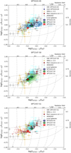 |
Fig. 16. L[CI](2 − 1)/LCO(7 − 6) versus L[CI](2 − 1)/LIR for our sources, SPT0103−45 (top) SPT2147−50 (middle), and SPT2357−51 (bottom). The global ratios of our sources are represented as squares. The pixel-wise ratios of our sources are represented as small dots. We note that since we use the data in each pixel and not each beam, the data points are not independent. The pixel-wise values are colour-coded based on the LIR of each pixel, with the darkest corresponding to the most luminous pixels. We compare our sources with the compilation presented in Valentino et al. (2020). The SMGs at z ∼ 2 − 4 are represented by golden stars (Walter et al. 2011; Alaghband-Zadeh et al. 2013; Bothwell et al. 2017; Yang et al. 2017; Andreani et al. 2018; Cañameras et al. 2018; Nesvadba et al. 2019; Dannerbauer et al. 2019; Jin et al. 2019). The main-sequence galaxies at z ∼ 1 are represented by maroon squares (Valentino et al. 2018, 2020; Bourne et al. 2019). The local FTS samples of star-forming galaxies are represented by aqua dots (Liu et al. 2015; Kamenetzky et al. 2014) and local FTS samples with AGN signatures are represented by grey diamonds (Véron-Cetty & Véron 2010; Liu et al. 2015; Kamenetzky et al. 2014). The grey dot-dashed and dashed lines are the isocontours of the UV radiation field (UUV) and the hydrogen density (nH) from the PDR models of Kaufman et al. (1999) in logarithmic values. |
Along with the ratios, in Fig. 16, we plot the radiation field and hydrogen volume density iso-contours from the photo dissociation region (PDR) modelling of Kaufman et al. (1999). The iso-density contours are mostly horizontal in this parameter space, indicating that the ratio between [CI](2−1) and CO(7−6) can be a proxy of the gas density. Similarly, the radiation-field iso-contours are almost vertical, indicating that the [CI](2−1)-to-LIR ratio is a proxy of the radiation field strength.
However, we should note that comparing the line ratios to PDR models does have caveats. There may be additional heating mechanisms that cannot be represented only with line ratios. The hot and dense PDRs can reproduce the line ratios but may not accurately reproduce the LIR as a part of the LIR may arise from the HII region. The internal properties and heating mechanisms of the sources may also be driven by the IR emission arising from the warm dust (Valentino et al. 2018).
The globally integrated ratios of our sources suggest that they have similar radiation field and densities to the compilation presented in Valentino et al. (2020). SPT0103−45 has the lowest density and radiation field strength of our three targets, while SPT2357−51 is our most extreme target in both parameters.
Turning to the pixel-wise ratios, we see that SPT0103−45 has a large variation in radiation field strength with almost uniform density, a result of the wide range in [CI]/LIR across the source. The gem region has a slightly higher radiation field strength and density compared to the global average. This region is likely a compact star-forming region close to the centre of the object (see Fig. 11). Inspection of Fig. 15 suggests that the regions closest to the gem have a stronger radiation field, possibly due to an elevated dust temperature or a high SFE producing more young stars and UV photons.
In SPT2147−50, we observe a fairly large dispersion in the gas density and the radiation field (∼0.5 dex). The kinematics and lensing reconstruction of the source (Sects. 5 and 6) suggest that the source could be a rotating disk. These variations of density could thus be caused by dynamical instabilities in this gas-rich system (Bournaud & Elmegreen 2009; Bournaud et al. 2009; Zanella et al. 2015).
The core of SPT2357−51 dominates the flux of the source (Fig. 15) and the associated pixels are very similar to the globally integrated ratios. In contrast, the outskirts of the system appear to have similar or lower densities, but higher radiation fields. Several explanations are possible. The centre of the object could be dustier, thereby preventing UV photons from penetrating the clouds. There could also be a dust temperature gradient from the outskirts to the center, which could bias our estimate of LIR and thus the radiation field strength (see Sect. 7.1).
8. Discussion
8.1. SPT0103–45
Despite having a complicated morphology in the image plane (Figs. 3 and 4) and an asymmetric observed integrated line profile (Fig. 1), SPT0103−45 seems to be compatible with a rotating disk from our lensing reconstruction (Sect. 6.4), with the asymmetry of the line profiles arising from differential magnification (Sect. 6.7).
The intrinsic SFR of SPT0103−45, after correcting for the continuum magnification derived in Sect. 6, is 1900 ± 600 M⊙ yr−1. Furthermore, using our continuum size estimates of the extended component, we compute the SFR surface density (ΣSFR) and find 69 ± 20 M⊙ yr−1 kpc−2. This is similar to typical SFR surface densities observed in SMGs (e.g. Daddi et al. 2010b; Casey et al. 2014).
We can also estimate the molecular gas mass from CO(3−2) observations from Reuter et al. (2020). We assume a CO(3−2)/CO(1−0) line ratio of 0.7 ± 0.1 from Harrington et al. (2021) and use an αCO = 3.4 M⊙ (K km s−1 pc2)−1 (where αCO is the CO-to-H2 conversion factor) from Jarugula et al. (2021). We note that the quoted value and uncertainty on the line ratio we assume is derived from and applicable to high-redshift SMGs only, the uncertainty would increase if we also considered other galaxy populations when making this assumption. In any case, we expect the uncertainty on αCO to dominate over the uncertainty in CO(3−1)/CO(1−0) line ratio. We find Mgas = (6.8 ± 2.1)×1011 M⊙ and a gas depletion timescale tdep = 360 ± 140 Myr. Instead, assuming a lower αCO = 0.8 (Downes & Solomon 1998), we find Mgas = (1.6 ± 0.5) × 1011 M⊙ and a gas depletion time scale tdep = 80 ± 40 Myr. This short depletion timescale is typical of starbursts (e.g. Daddi et al. 2010b; Béthermin et al. 2015).
Furthermore, we estimate the dynamical mass of the system using a simple approach. Assuming a simple circular Keplerian motion, the enclosed dynamical mass Mdyn can be computed using the following equation:
 (4)
(4)
where R is the radius, which we take to be half of the distance between the lowest and highest velocity components in the source plane (see Table C.2). We estimated the inclination i of the system using the b/a ratio of the continuum model (cos i = b/a). Vobs is the projected component of the circular velocity along the line of sight and is computed as half of the velocity difference between the two extreme velocity bins. This approach is an intermediate between the crude estimate based on the line width and the size (e.g. Aravena et al. 2016; Bothwell et al. 2017; Dessauges-Zavadsky et al. 2020) and a full dynamical approach (e.g. Rizzo et al. 2020; Jones et al. 2021) done on higher resolution data or unlensed objects. Contrary to the crude approach, we can take the inclination of our objects into account and obtain the circular velocity in the outskirts of the objects instead of an integrated line width. Of course, it relies on the strong assumption that these systems are dynamically relaxed disks.
We estimate the uncertainties on the result by computing Mdyn for all realisations of MCMC chains from the lens model, though we expect that systematic uncertainties in, for instance, the assumed source geometry are dominant. We find a dynamical mass Mdyn of (1.2 ± 0.5) × 1011 M⊙ using the CO(7−6) radius and velocities and (1.55 ± 0.4)×1011 M⊙ using the [CI](2−1) radius and velocities.
We find compatible values between this dynamical mass and the molecular gas mass using the lower αCO = 0.8 value. Under this assumption there is only a small difference between the dynamical and gas masses, implying that the stellar mass of the source is relatively low. We note that the dynamical mass is calculated with the radius of the mid-J CO transition which requires higher excitation temperatures, typically found in the galactic centers. In Fig. 17, the depletion timescale of SPT0103−45 is similar to the bulk SMG population. However, the short depletion time and the high SFR density corresponds to a starburst-like star formation mode, which is usually not expected in isolated disks. An αCO = 3.4 (∼4) leads to a longer depletion timescale usually found in disk galaxies, but this would also result in a strong tension with the dynamical mass. Only higher resolution data could allow us to identify a potential interaction triggering the starburst. We also cannot exclude processes linked to disk instabilities (e.g. Bournaud et al. 2007).
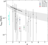 |
Fig. 17. The depletion timescale versus redshift of our sources, compared with other SPT-SMGs and other high-z SMGs. The depletion timescales for our sources are computed with the gas mass estimated from low-J CO fluxes with an αCO = 0.8. The grey shaded region represents the evolution of the depletion timescale with redshifts for main sequence galaxies. This plot is adapted from Jarugula et al. (2021). The high-redshift gravitationally lensed SPT-SMGs are from Aravena et al. (2016) and Reuter et al. (2020) and the other high-redshift SMGs are taken from Carilli et al. (2010), Walter et al. (2012), Fu et al. (2012, 2013), Ivison et al. (2013), Alaghband-Zadeh et al. (2013). The main sequence galaxies are described in Saintonge et al. (2013) as tdep = 1.5 (1 + z) α, where α is from −1.5 (Davé et al. 2012) to −1.0 (Magnelli et al. 2013), which is shown as the grey shaded region. |
8.2. SPT2147−50
The dynamics of SPT2147−50 are similar to SPT0103−45, with our source plane modelling being compatible with rotation. SPT2147−50 has a lensing-corrected SFR of 830 ± 200 M⊙ yr−1 and a ΣSFR of 30 ± 7 M⊙ yr−1 kpc−2. Bothwell et al. (2017) estimated the molecular gas mass using [CI](1−0) and found Mmol = (6.8 ± 0.5)×1010 M⊙ (after updating their magnification by our [CI](2−1)-based measurement). Aravena et al. (2016) found a smaller molecular gas mass of (2.3 ± 0.5)×1010 M⊙ using CO(2−1) (αCO = 0.8,  and updating the magnification using our CO(7−6)-based value). We derive a depletion timescale tdep = 82 ± 7 Myr using [CI](1−0) and tdep = 28 ± 9 Myr using CO(2−1). This short depletion timescale is usually associated to a starburst. If instead we compute the gas mass using a Milky Way-like αCO = 3.4, we find a gas mass of (9.9 ± 0.5)×1010 M⊙ and a depletion time tdep = 119 ± 29 Myr.
We can also compute the dynamical mass of the system using the same method as SPT0103−45. We find Mdyn = (2.5 ± 0.4)×1010 M⊙ from the CO(7−6) data and Mdyn = (3.4 ± 0.4) × 1010 M⊙ using [CI](2−1). This is very similar to a comparable dynamical estimate from Aravena et al. (2016) using only the line width and the continuum effective radius. We note that the estimate of the gas mass from CO(2−1) and using αCO = 0.8 seems to agree better with the dynamical mass than the [CI]-derived ones. In Fig. 17, we see that the depletion timescale is somewhat shorter compared to the bulk of the SMGs. Similar to SPT0103−45, using αCO = 3.4 leads to tension between the gas and dynamical masses.
8.3. SPT2357−51
The most interesting feature of this compact source is the double-peak profile of the spectrum (Fig. 1, bottom panel) seen for both lines. The PV diagram of the source (see Fig. 8), the image plane spectral modelling of the source with two components (Sect. 5.3) and the lens reconstruction (Sect. 6.6) suggest a merger between two components. The intrinsic flux ratio between the two components are 0.5:1 and 0.84:1 in CO(7−6) and [CI](2−1), respectively, with the blue component being brighter.
The blue component shows a smooth velocity gradient for both lines suggesting possible rotation or tidal streaming motions, whereas the red component exhibits a much more disturbed velocity structure. Comparing the positions of these components with the continuum emission, we notice that the red component is more centred on the continuum than the blue component. This could indicate a difference in their dust properties, with the red component being more dusty than the blue one. This could indicate a different chemical maturity of the two components which might be merging. However, it is surprising that the dustier component is the less massive one, since usually more massive galaxies are also dustier (Heinis et al. 2014; Fudamoto et al. 2020).
Using the magnification factor obtained from our continuum best-fit lens model and the LIR from Reuter et al. (2020), we compute an intrinsic SFR of 1620 ± 260 M⊙ yr−1. Based on the continuum source size from the lens modelling (Sect. 6.6), we estimate the SFR density ΣSFR to be 59 ± 10 M⊙ yr−1 kpc−2, which is similar to the other sources and typical of SMGs.
We also estimate the gas mass of the system from the CO(3−2) flux measurement from Reuter et al. (2020). Using a CO(3−2)/CO(1−0) conversion factor of 0.7 ± 0.1 from Harrington et al. (2021) and αCO = 3.4, we obtain Mgas = (1.6 ± 0.5) × 1011 M⊙ and a depletion timescale tdep = 99 ± 29 Myr. Alternatively, using an αCO = 0.8, we obtain Mgas = (3.9 ± 1.3)×1010 M⊙ and a very short depletion timescale tdep = 24 ± 9 Myr. This is much lower than the depletion timescales of the bulk of the SMG population shown in Fig. 17. Such short depletion times have also been measured in some extreme lensed SMGs but remain unusual (Béthermin et al. 2016; Ciesla et al. 2020). This reinforces the hypothesis that SPT2357−51 is an extreme starburst possibly triggered by a major merger. We do not calculate the dynamical mass of the system as we cannot assume that it is a dynamically relaxed system.
9. Conclusions
In this paper, we presented high-resolution ALMA spectral imaging of a sample of three DSFGs: SPT0103−45, SPT2147−50 and SPT2357−51. We characterised the gas reservoirs, kinematics and morphology of the sample. We performed pixel-wise velocity decomposition, visibility-based lens modelling and ratio analyses of the line and continuum emission of our sources. Our main conclusions are:
-
All the sources have high intrinsic SFRs > 800 M⊙ yr−1.
-
Our sources have comparable ISM radiation field intensities and densities as other SMGs.
-
The CO(7−6)/[CI](2−1) luminosity ratios are lower than in the lensed SMGs presented in Andreani et al. (2018) and Yang et al. (2017).
-
SPT0103−45 and SPT2147−50 are consistent with rotating starbursts with short depletion scales (< 100 Myr). However, since our tracers predominantly trace cold gas, we cannot exclude the possibility of merging with a mostly ionised or low-magnification component.
-
The dynamical mass is compatible with the gas mass of these two sources estimated assuming αCO = 0.8 but not Milky Way like values. A higher αCO results in the gas mass being much larger than the dynamical mass, which is not physical.
-
SPT2357−51 could possibly be an ongoing merger. The red and the blue components seen in the Gaussian decomposition are intrinsically different. This source is a strong starburst with a short depletion timescale of 26 ± 5 Myr.
This small sample demonstrates how powerful spatially and spectrally resolved multi-line ALMA observations can be in unveiling the nature of high-z lensed starbursts. Our analysis reveals a diversity in the morphology and dynamics of SMGs, in agreement with simulations (e.g. Hayward et al. 2011). With larger samples, more emission lines, and higher spatial resolution, we will be able to better characterise the ISM of such massive galaxies and probe into the diversity of the population.
We note that the [CI](2−1) line was also tentatively detected and broad in the initial data reduction of the APEX spectra used to write the ALMA proposal.
SPT2147−50 has only one spectral window centred on the lines with 7.813 MHz resolution. The second spectral window in the sideband has a coarser resolution (31.25 MHz).
Note that the factor relating to the spatial distribution of dust is referred to as β in Cochrane et al. (2019). We chose to refer to it using the symbol γ to avoid confusions with the dust emissivity index.
After converting from L′ (K km s−1 pc2) to L (L⊙) units.
Acknowledgments
We thank Francesco Valentino for providing the data associated with his [CI] data compilation. We thank Zhi-Yu Zhang for sharing his GILDAS/CLASS script to automatically flag bad APEX data. This paper makes use of the following ALMA data: ADS/JAO.ALMA#2017.1.01018.S, ADS/JAO.ALMA#2018.1.01060.S. ALMA is a partnership of ESO (representing its member states), NSF (USA) and NINS (Japan), together with NRC (Canada), MOST and ASIAA (Taiwan) and KASI (Republic of Korea), in cooperation with the Republic of Chile. The Joint ALMA Observatory is operated by ESO, AUI/NRAO and NAOJ. The National Radio Astronomy Observatory is a facility of the National Science Foundation operated under cooperative agreement by Associated Universities, Inc. This publication is based on data acquired with the Atacama Pathfinder Experiment (APEX). APEX is a collaboration between the Max-Planck-Institut fur Radioastronomie, the European Southern Observatory and the Onsala Space Observatory. Based on observations made with ESO Telescopes at the La Silla Paranal Observatory under programmeme ID 097.A-0973. This work was supported by the programmeme National “Physique et Chimie du Milieu Interstellaire” (PCMI) of CNRS/INSU with INC/INP co-funded by CEA and CNES. This work was supported by the programmeme National Cosmology et Galaxies (PNCG) of CNRS/INSU with INP and IN2P3, co-funded by CEA and CNES. J.S.S is supported by NASA Hubble Fellowship grant #HF2-51446 awarded by the Space Telescope Science Institute, which is operated by the Association of Universities for Research in Astronomy, Inc., for NASA, under contract NAS5-26555. M.A. acknowledges support from FONDECYT grant 1211951, ANID+PCI+INSTITUTO MAX PLANCK DE ASTRONOMIA MPG 190030, ANID+PCI+REDES 190194 and ANID BASAL project FB210003. M.A.A. and J.V. acknowledge support from the center for AstroPhysical Surveys at the National Center for Supercomputing Applications in Urbana, IL. J.V. acknowledges support from the Sloan Foundation.
References
- Alaghband-Zadeh, S., Chapman, S. C., Swinbank, A. M., et al. 2013, MNRAS, 435, 1493 [Google Scholar]
- Andreani, P., Retana-Montenegro, E., Zhang, Z.-Y., et al. 2018, A&A, 615, A142 [NASA ADS] [CrossRef] [EDP Sciences] [Google Scholar]
- Apostolovski, Y., Aravena, M., Anguita, T., et al. 2019, A&A, 628, A23 [NASA ADS] [CrossRef] [EDP Sciences] [Google Scholar]
- Aravena, M., Spilker, J. S., Bethermin, M., et al. 2016, MNRAS, 457, 4406 [Google Scholar]
- Belitsky, V., Lapkin, I., Fredrixon, M., et al. 2018, A&A, 612, A23 [NASA ADS] [CrossRef] [EDP Sciences] [Google Scholar]
- Béthermin, M., Daddi, E., Magdis, G., et al. 2015, A&A, 573, A113 [Google Scholar]
- Béthermin, M., De Breuck, C., Gullberg, B., et al. 2016, A&A, 586, L7 [NASA ADS] [CrossRef] [EDP Sciences] [Google Scholar]
- Béthermin, M., Greve, T. R., De Breuck, C., et al. 2018, A&A, 620, A115 [NASA ADS] [CrossRef] [EDP Sciences] [Google Scholar]
- Béthermin, M., Fudamoto, Y., Ginolfi, M., et al. 2020, A&A, 643, A2 [Google Scholar]
- Bisbas, T. G., Papadopoulos, P. P., & Viti, S. 2015, ApJ, 803, 37 [NASA ADS] [CrossRef] [Google Scholar]
- Bolatto, A. D., Wolfire, M., & Leroy, A. K. 2013, ARA&A, 51, 207 [CrossRef] [Google Scholar]
- Bothwell, M. S., Smail, I., Chapman, S. C., et al. 2013, MNRAS, 429, 3047 [Google Scholar]
- Bothwell, M. S., Aguirre, J. E., Aravena, M., et al. 2017, MNRAS, 466, 2825 [Google Scholar]
- Bournaud, F., & Elmegreen, B. G. 2009, ApJ, 694, L158 [CrossRef] [Google Scholar]
- Bournaud, F., Elmegreen, B. G., & Elmegreen, D. M. 2007, ApJ, 670, 237 [Google Scholar]
- Bournaud, F., Elmegreen, B. G., & Martig, M. 2009, ApJ, 707, L1 [Google Scholar]
- Bourne, N., Dunlop, J. S., Simpson, J. M., et al. 2019, MNRAS, 482, 3135 [Google Scholar]
- Briggs, D. S. 1995, Am. Astron. Soc. Meet. Abstr., 187, 112.02 [Google Scholar]
- Bussmann, R. S., Riechers, D., Fialkov, A., et al. 2015, ApJ, 812, 43 [Google Scholar]
- Calistro Rivera, G., Hodge, J. A., Smail, I., et al. 2018, ApJ, 863, 56 [Google Scholar]
- Cañameras, R., Nesvadba, N. P. H., Guery, D., et al. 2015, A&A, 581, A105 [Google Scholar]
- Cañameras, R., Yang, C., Nesvadba, N. P. H., et al. 2018, A&A, 620, A61 [Google Scholar]
- Carilli, C. L., & Walter, F. 2013, ARA&A, 51, 105 [NASA ADS] [CrossRef] [Google Scholar]
- Carilli, C. L., Daddi, E., Riechers, D., et al. 2010, ApJ, 714, 1407 [NASA ADS] [CrossRef] [Google Scholar]
- Carlstrom, J. E., Ade, P. A. R., Aird, K. A., et al. 2011, PASP, 123, 568 [CrossRef] [Google Scholar]
- Casey, C. M., Narayanan, D., & Cooray, A. 2014, Phys. Rep., 541, 45 [Google Scholar]
- Chabrier, G. 2003, PASP, 115, 763 [Google Scholar]
- Chun, K., Smith, R., Shin, J., Kim, S. S., & Raouf, M. 2020, ApJ, 889, 173 [NASA ADS] [CrossRef] [Google Scholar]
- Cicone, C., Maiolino, R., Sturm, E., et al. 2014, A&A, 562, A21 [NASA ADS] [CrossRef] [EDP Sciences] [Google Scholar]
- Ciesla, L., Béthermin, M., Daddi, E., et al. 2020, A&A, 635, A27 [NASA ADS] [CrossRef] [EDP Sciences] [Google Scholar]
- Cochrane, R. K., Hayward, C. C., Anglés-Alcázar, D., et al. 2019, MNRAS, 488, 1779 [NASA ADS] [CrossRef] [Google Scholar]
- Conway, J. E., Cornwell, T. J., & Wilkinson, P. N. 1990, MNRAS, 246, 490 [Google Scholar]
- da Cunha, E., Walter, F., Smail, I. R., et al. 2015, ApJ, 806, 110 [Google Scholar]
- Daddi, E., Bournaud, F., Walter, F., et al. 2010a, ApJ, 713, 686 [NASA ADS] [CrossRef] [Google Scholar]
- Daddi, E., Elbaz, D., Walter, F., et al. 2010b, ApJ, 714, L118 [NASA ADS] [CrossRef] [Google Scholar]
- Dannerbauer, H., Harrington, K., Díaz-Sánchez, A., et al. 2019, AJ, 158, 34 [Google Scholar]
- Davé, R., Finlator, K., & Oppenheimer, B. D. 2012, MNRAS, 421, 98 [Google Scholar]
- Dekel, A., Birnboim, Y., Engel, G., et al. 2009, Nature, 457, 451 [Google Scholar]
- Dessauges-Zavadsky, M., Zamojski, M., Schaerer, D., et al. 2015, A&A, 577, A50 [NASA ADS] [CrossRef] [EDP Sciences] [Google Scholar]
- Dessauges-Zavadsky, M., Ginolfi, M., Pozzi, F., et al. 2020, A&A, 643, A5 [NASA ADS] [CrossRef] [EDP Sciences] [Google Scholar]
- Dong, C., Spilker, J. S., Gonzalez, A. H., et al. 2019, ApJ, 873, 50 [NASA ADS] [CrossRef] [Google Scholar]
- Downes, D., & Solomon, P. M. 1998, ApJ, 507, 615 [NASA ADS] [CrossRef] [Google Scholar]
- Dunne, L., Maddox, S. J., Vlahakis, C., & Gomez, H. L. 2021, MNRAS, 501, 2573 [NASA ADS] [CrossRef] [Google Scholar]
- Dye, S., Furlanetto, C., Swinbank, A. M., et al. 2015, MNRAS, 452, 2258 [NASA ADS] [CrossRef] [Google Scholar]
- Faisst, A. L., Schaerer, D., Lemaux, B. C., et al. 2020, ApJS, 247, 61 [NASA ADS] [CrossRef] [Google Scholar]
- Fixsen, D. J., Bennett, C. L., & Mather, J. C. 1999, ApJ, 526, 207 [Google Scholar]
- Florez, J., Jogee, S., Guo, Y., et al. 2021, MNRAS, 508, 762 [NASA ADS] [CrossRef] [Google Scholar]
- Fu, H., Jullo, E., Cooray, A., et al. 2012, ApJ, 753, 134 [NASA ADS] [CrossRef] [Google Scholar]
- Fu, H., Cooray, A., Feruglio, C., et al. 2013, Nature, 498, 338 [CrossRef] [Google Scholar]
- Fudamoto, Y., Oesch, P. A., Faisst, A., et al. 2020, A&A, 643, A4 [NASA ADS] [CrossRef] [EDP Sciences] [Google Scholar]
- Fujimoto, S., Silverman, J. D., Bethermin, M., et al. 2020, ApJ, 900, 1 [Google Scholar]
- Genzel, R., Tacconi, L. J., Gracia-Carpio, J., et al. 2010, MNRAS, 407, 2091 [NASA ADS] [CrossRef] [Google Scholar]
- Ginolfi, M., Jones, G. C., Béthermin, M., et al. 2020, A&A, 633, A90 [NASA ADS] [CrossRef] [EDP Sciences] [Google Scholar]
- Greve, T. R., Bertoldi, F., Smail, I., et al. 2005, MNRAS, 359, 1165 [NASA ADS] [CrossRef] [Google Scholar]
- Greve, T. R., Vieira, J. D., Weiß, A., et al. 2012, ApJ, 756, 101 [NASA ADS] [CrossRef] [Google Scholar]
- Harrington, K. C., Weiss, A., Yun, M. S., et al. 2021, ApJ, 908, 95 [NASA ADS] [CrossRef] [Google Scholar]
- Harris, A. I., Baker, A. J., Frayer, D. T., et al. 2012, ApJ, 752, 152 [NASA ADS] [CrossRef] [Google Scholar]
- Hayward, C. C., Kereš, D., Jonsson, P., et al. 2011, ApJ, 743, 159 [CrossRef] [Google Scholar]
- Heinis, S., Buat, V., Béthermin, M., et al. 2014, MNRAS, 437, 1268 [Google Scholar]
- Hezaveh, Y. D., Marrone, D. P., & Holder, G. P. 2012, ApJ, 761, 20 [NASA ADS] [CrossRef] [Google Scholar]
- Hezaveh, Y. D., Dalal, N., Marrone, D. P., et al. 2016, ApJ, 823, 37 [Google Scholar]
- Hodge, J. A., Karim, A., Smail, I., et al. 2013, ApJ, 768, 91 [Google Scholar]
- Ivison, R. J., Smail, I., Amblard, A., et al. 2012, MNRAS, 425, 1320 [NASA ADS] [CrossRef] [Google Scholar]
- Ivison, R. J., Swinbank, A. M., Smail, I., et al. 2013, ApJ, 772, 137 [NASA ADS] [CrossRef] [Google Scholar]
- Jarugula, S., Vieira, J. D., Weiß, A., et al. 2021, ApJ, 921, 97 [NASA ADS] [CrossRef] [Google Scholar]
- Jin, S., Daddi, E., Magdis, G. E., et al. 2019, ApJ, 887, 144 [Google Scholar]
- Jones, G. C., Vergani, D., Romano, M., et al. 2021, MNRAS, 507, 3540 [NASA ADS] [CrossRef] [Google Scholar]
- Kamenetzky, J., Rangwala, N., Glenn, J., Maloney, P. R., & Conley, A. 2014, ApJ, 795, 174 [Google Scholar]
- Karim, A., Swinbank, A. M., Hodge, J. A., et al. 2013, MNRAS, 432, 2 [Google Scholar]
- Kaufman, M. J., Wolfire, M. G., Hollenbach, D. J., & Luhman, M. L. 1999, ApJ, 527, 795 [Google Scholar]
- Keene, J., Blake, G. A., Phillips, T. G., Huggins, P. J., & Beichman, C. A. 1985, ApJ, 299, 967 [NASA ADS] [CrossRef] [Google Scholar]
- Kennicutt, R. C., Jr. 1998, ARA&A, 36, 189 [Google Scholar]
- Kennicutt, R. C., & Evans, N. J. 2012, ARA&A, 50, 531 [NASA ADS] [CrossRef] [Google Scholar]
- Kleiner, D., Pimbblet, K. A., Jones, D. H., Koribalski, B. S., & Serra, P. 2017, MNRAS, 466, 4692 [Google Scholar]
- Kretschmer, M., Agertz, O., & Teyssier, R. 2020, MNRAS, 497, 4346 [NASA ADS] [CrossRef] [Google Scholar]
- Langer, W. 1976, ApJ, 206, 699 [NASA ADS] [CrossRef] [Google Scholar]
- Le Fèvre, O., Béthermin, M., Faisst, A., et al. 2020, A&A, 643, A1 [Google Scholar]
- Litke, K. C., Marrone, D. P., Spilker, J. S., et al. 2019, ApJ, 870, 80 [Google Scholar]
- Liu, D., Gao, Y., Isaak, K., et al. 2015, ApJ, 810, L14 [NASA ADS] [CrossRef] [Google Scholar]
- Magdis, G. E., Rigopoulou, D., Daddi, E., et al. 2017, A&A, 603, A93 [NASA ADS] [CrossRef] [EDP Sciences] [Google Scholar]
- Magnelli, B., Popesso, P., Berta, S., et al. 2013, A&A, 553, A132 [NASA ADS] [CrossRef] [EDP Sciences] [Google Scholar]
- Maiolino, R., Gallerani, S., Neri, R., et al. 2012, MNRAS, 425, L66 [Google Scholar]
- Marsden, D., Gralla, M., Marriage, T. A., et al. 2014, MNRAS, 439, 1556 [NASA ADS] [CrossRef] [Google Scholar]
- McMullin, J. P., Waters, B., Schiebel, D., Young, W., & Golap, K. 2007, in Astronomical Data Analysis Software and Systems XVI, eds. R. A. Shaw, F. Hill, & D. J. Bell, ASP Conf. Ser., 376, 127 [Google Scholar]
- Narayanan, D., & Krumholz, M. R. 2014, MNRAS, 442, 1411 [NASA ADS] [CrossRef] [Google Scholar]
- Negrello, M., Hopwood, R., De Zotti, G., et al. 2010, Science, 330, 800 [NASA ADS] [CrossRef] [Google Scholar]
- Nesvadba, N. P. H., Cañameras, R., Kneissl, R., et al. 2019, A&A, 624, A23 [NASA ADS] [CrossRef] [EDP Sciences] [Google Scholar]
- Omont, A. 2007, Rep. Progr. Phys., 70, 1099 [Google Scholar]
- Oteo, I., Zhang, Z. Y., Yang, C., et al. 2017, ApJ, 850, 170 [NASA ADS] [CrossRef] [Google Scholar]
- Pantoni, L., Massardi, M., Lapi, A., et al. 2021, MNRAS, 507, 3998 [CrossRef] [Google Scholar]
- Papadopoulos, P. P., & Greve, T. R. 2004, ApJ, 615, L29 [Google Scholar]
- Papadopoulos, P. P., Thi, W. F., & Viti, S. 2004, MNRAS, 351, 147 [NASA ADS] [CrossRef] [Google Scholar]
- Paraficz, D., Rybak, M., McKean, J. P., et al. 2018, A&A, 613, A34 [NASA ADS] [CrossRef] [EDP Sciences] [Google Scholar]
- Reuter, C., Vieira, J. D., Spilker, J. S., et al. 2020, ApJ, 902, 78 [NASA ADS] [CrossRef] [Google Scholar]
- Rizzo, F., Vegetti, S., Powell, D., et al. 2020, Nature, 584, 201 [Google Scholar]
- Saintonge, A., Lutz, D., Genzel, R., et al. 2013, ApJ, 778, 2 [Google Scholar]
- Serjeant, S. 2012, MNRAS, 424, 2429 [NASA ADS] [CrossRef] [Google Scholar]
- Sérsic, J. L. 1968, https://doi.org/10.5281/zenodo.2562394 [Google Scholar]
- Solomon, P. M., & Vanden Bout, P. A. 2005, ARA&A, 43, 677 [NASA ADS] [CrossRef] [Google Scholar]
- Solomon, P. M., Downes, D., & Radford, S. J. E. 1992, ApJ, 398, L29 [Google Scholar]
- Spilker, J. S., Aravena, M., Marrone, D. P., et al. 2015, ApJ, 811, 124 [NASA ADS] [CrossRef] [Google Scholar]
- Spilker, J. S., Marrone, D. P., Aravena, M., et al. 2016, ApJ, 826, 112 [NASA ADS] [CrossRef] [Google Scholar]
- Spilker, J. S., Phadke, K. A., Aravena, M., et al. 2020a, ApJ, 905, 85 [Google Scholar]
- Spilker, J. S., Aravena, M., Phadke, K. A., et al. 2020b, ApJ, 905, 86 [Google Scholar]
- Strandet, M. L., Weiss, A., Vieira, J. D., et al. 2016, ApJ, 822, 80 [NASA ADS] [CrossRef] [Google Scholar]
- Swinbank, A. M., Simpson, J. M., Smail, I., et al. 2014, MNRAS, 438, 1267 [Google Scholar]
- Tacconi, L. J., Genzel, R., Neri, R., et al. 2010, Nature, 463, 781 [Google Scholar]
- Tacconi, L. J., Neri, R., Genzel, R., et al. 2013, ApJ, 768, 74 [NASA ADS] [CrossRef] [Google Scholar]
- Tan, Q., Daddi, E., Magdis, G., et al. 2014, A&A, 569, A98 [NASA ADS] [CrossRef] [EDP Sciences] [Google Scholar]
- Tielens, A. G. G. M., & Hollenbach, D. 1985, ApJ, 291, 722 [Google Scholar]
- Tomassetti, M., Porciani, C., Romano-Diaz, E., Ludlow, A. D., & Papadopoulos, P. P. 2014, MNRAS, 445, L124 [NASA ADS] [CrossRef] [Google Scholar]
- Tunnard, R., & Greve, T. R. 2016, ApJ, 819, 161 [NASA ADS] [CrossRef] [Google Scholar]
- Valentino, F., Magdis, G. E., Daddi, E., et al. 2018, ApJ, 869, 27 [Google Scholar]
- Valentino, F., Magdis, G. E., Daddi, E., et al. 2020, ApJ, 890, 24 [Google Scholar]
- Véron-Cetty, M. P., & Véron, P. 2010, A&A, 518, A10 [Google Scholar]
- Vieira, J. D., Crawford, T. M., Switzer, E. R., et al. 2010, ApJ, 719, 763 [NASA ADS] [CrossRef] [Google Scholar]
- Vieira, J. D., Marrone, D. P., Chapman, S. C., et al. 2013, Nature, 495, 344 [Google Scholar]
- Walter, F., Weiß, A., Downes, D., Decarli, R., & Henkel, C. 2011, ApJ, 730, 18 [Google Scholar]
- Walter, F., Decarli, R., Carilli, C., et al. 2012, ApJ, 752, 93 [CrossRef] [Google Scholar]
- Weiß, A., Henkel, C., Downes, D., & Walter, F. 2003, A&A, 409, L41 [NASA ADS] [CrossRef] [EDP Sciences] [Google Scholar]
- Weiß, A., Downes, D., Walter, F., & Henkel, C. 2005, A&A, 440, L45 [Google Scholar]
- Weiß, A., Downes, D., Neri, R., et al. 2007, A&A, 467, 955 [NASA ADS] [CrossRef] [EDP Sciences] [Google Scholar]
- Yang, C., Omont, A., Beelen, A., et al. 2017, A&A, 608, A144 [NASA ADS] [CrossRef] [EDP Sciences] [Google Scholar]
- Zanella, A., Daddi, E., Le Floc’h, E., et al. 2015, Nature, 521, 54 [Google Scholar]
Appendix A: High-resolution continuum image of SPT2357-51
To visualise the continuum emission of SPT2357-51 at higher resolution than our default imaging scheme, we imaged the continuum data using only the visibilities on the longest baselines, as it samples the structure of the galaxy on the smallest scales. Figure A.1 shows the continuum image of SPT2357-51 created using only the data from baselines > 200 kλ. The spatial resolution of this image is 0.31×0.24″. We note that this image is merely for illustrative purposes because our lens modelling procedure fits directly to the visibilities, which are not affected by choices in imaging parameters.
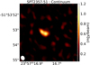 |
Fig. A.1. The continuum image of SPT2357-51 imaged using the data from baselines > 200 kλ, demonstrating the resolved structure of the galaxy and its agreement with the results of our gravitational lens modelling. |
Appendix B: De-blending the spectra of SPT0103-45
From Fig. 1 (top panel), we see that the redshifted tail of [CI](2-1) emission is blended with the CO(7-6) line. Hence we deblended these lines using multiple-Gaussian fitting, as described further in the text. We fit the CO and [CI] lines with three Gaussian profiles each, but fixed the central velocity and line width to be equal for both CO and [CI]. The resulting fit uses 12 free parameters: six Gaussian amplitudes, three central velocities, and three line widths. In the resulting best-fit line profiles (Figure B.1), we find a narrow overlap region where both CO and [CI] contribute, near ∼ + 800 km/s relative to CO(7-6). In our spatially resolved line ratio analysis, we simply divided the two lines using the frequency ranges shown in Figure 1. Compared to that method, a more detailed accounting of the line blending results in a higher CO/[CI] line ratio by ≈5%, a < 2 σ difference. This small difference is taken into account by combining the statistical uncertainties with a 5% systematic error.
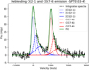 |
Fig. B.1. The Gaussian deblending of the CO and [CI] spectrum of SPT0103-45. Each of the lines are fitted with 3 Gaussian profiles. The blue fit represents the [CI](2-1) line and the red fit is the CO(7-6) line fit. The green line represents the total of both lines. |
Appendix C: Lens modelling parameters
The best-fit parameters of the lensing potential and the source profiles are tabulated in Table C.1.
Lens parameters.
Intrinsic properties of SPT0103-45.
Intrinsic properties of SPT2147-50.
Intrinsic properties of SPT2357-51.
Appendix D: Differential magnification – Intrinsic versus observed spectra for our sources
Figure D.1 shows the intrinsic spectra (from the lens modelling of the velocity bins for our sources) compared with the observed spectra.
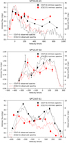 |
Fig. D.1. The intrinsic spectra for the [CI](2-1) line (red filled squares) and the CO(7-6) line (black filled circles). The top panel shows the results for SPT0103-45. The middle panel shows the results of SPT2147-50 and the bottom panel for SPT2357-51. We overplot the observed spectra using a dashed-line, red for [CI](2-1) and black for CO(7-6). |
Appendix E: Comparison between the data and the lens model in the various velocity bins
To check the agreement between our data and the lens model, we plot the dirty image of our sources in every velocity bin along with the models corresponding to the data.
SPT0103-45
The number of counter images and the source structure in the image plane varies across the velocities. In Fig. E.1 and Fig. E.2 we can see a single image in the higher velocities and two counter images in the lower velocities. We also see a nice agreement between the data and the model.
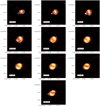 |
Fig. E.1. SPT0103-45 model-dirty images of [CI](2-1) for every velocity bin are plotted along with the 3, 5, and 7 σ contours of the dirty image. The central velocities corresponding to each of the bins are mentioned in the figures. |
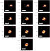 |
Fig. E.2. SPT0103-45 model-dirty image of CO(7-6) for every velocity bins is plotted along with the 3, 5, and 7 σ contours of the dirty image. The central velocity corresponding to each of the bin is mentioned in the figures. |
SPT2147-50
In Fig. E.3 and Fig. E.4, we see a good agreement between the data and the model across the velocities. The dirty image and the number of counter images vary across the velocity bins, similar to SPT0103-45. For the low velocity regions, we do not see the arc in the north, which is seen in the continuum and the higher velocity bins.
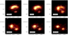 |
Fig. E.3. SPT2147-50 model-dirty image of [CI](2-1) for every velocity bins is plotted along with the 3, 5, and 7 σ contours of the dirty image. The central velocities corresponding to each of the bins are mentioned in the figures. |
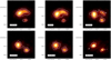 |
Fig. E.4. SPT2147-50 model-dirty image of CO(7-6) for every velocity bins is plotted along with the 3, 5, and 7 σ contours of the dirty image. The central velocities corresponding to each of the bins are mentioned in the figures. |
SPT2357-51
Similar to our other sources, we see a good agreement between the data and the model in Fig. E.5 and Fig. E.6. SPT2357-51 shows no counter images across the velocities for both of the lines.
 |
Fig. E.5. SPT2357-51 model-dirty image of [CI](2-1) for every velocity bins is plotted along with the 3, 5, and 7 σ contours of the dirty image. The central velocities corresponding to each of the bins are mentioned in the figures. |
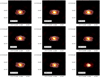 |
Fig. E.6. SPT2357-51 model-dirty image of CO(7-6) for every velocity bins is plotted along with the 3, 5, and 7 σ contours of the dirty image. The central velocities corresponding to each of the bins are mentioned in the figures. |
All Tables
All Figures
|
Fig. 1. Integrated spectra of SPT0103−45 (top panel), SPT2147−50 (middle panel) and SPT2357−51 (lower panel). The black solid line is the spectrum extracted from the ALMA observations (see Sect. 2.3). The light grey line is the APEX/SEPIA spectrum (see Sect. 2.1). Red and blue vertical dashed lines indicate the position of CO(7−6) and [CI](2−1) lines, respectively, at the reference redshift of the source. The yellow and cyan shaded areas show the integration windows used to compute integrated fluxes of the CO(7−6) and [CI](2−1) lines, respectively (see Sect. 4.3). The zero-velocity corresponds to the observed frequency of CO(7−6) line for each of the sources. |
| In the text | |
|
Fig. 2. Line luminosity of [CI](2−1) (top-panel) and CO(7−6) (bottom-panel) vs. infrared luminosity. All the luminosities in this plot are not corrected for magnification. Our sources (filled squares) are compared with the SMGs (stars), main-sequence at z ∼ 1 (diamonds), local galaxies (dots), AGN and QSO (hexagons) from the compilation of Valentino et al. (2020). |
| In the text | |
|
Fig. 3. Continuum and moment-0 maps of our sample. First row: continuum maps of (from left to right) SPT0103−45, SPT2147−50, and SPT2357−51 (see Sect. 3.2). The synthesised beam is represented as the white ellipse on the bottom left of every map. Second row: is the integrated [CI](2−1) intensity maps. Third row: is the integrated CO(7−6) intensity maps of our sources (see Sect. 4.3). |
| In the text | |
|
Fig. 4. Properties of the ‘gem’ in SPT0103−45. Left panel: is the continuum map as described in Sect. 3.2. The white line shows the direction along with the slice for the PV diagram is extracted (Fig. 6). The spectrum shown in the centre panel is extracted at the coordinates of the gem (Sect. 3.3). The frequency range represented by the yellow region is used to compute the integrated intensity of the high-velocity emission, represented in the right panel. The white contours are the 5, 10 and 15σ contours of the continuum emission. |
| In the text | |
|
Fig. 5. Pixel-wise peak velocity decomposition of SPT0103−45. Top row: velocity map of the [CI](2−1) line and bottom row: CO(7−6) line. The 5, 10, and 15σ contours of the continuum emission are plotted on all velocity maps. The construction of these maps is described in Sect. 5.1. |
| In the text | |
|
Fig. 6. Position-velocity diagram of SPT0103−45. The axis used to make this diagram is shown in the first panel of Fig. 4. The velocity axis on the left y-axis has the zero-velocity of the CO(7−6) observed frequency and the right y-axis has the zero-velocity centred at the [CI](2−1) observed frequency. |
| In the text | |
|
Fig. 7. Pixel-wise peak velocity decomposition of SPT2147−50. The velocity maps of [CI](2−1) (left) and CO(7−6) (right) are shown. The 3, 5, and 10σ contours of the continuum are overplotted on the velocity maps. The construction of these maps are described in Sect. 5.2 |
| In the text | |
|
Fig. 8. The position-velocity diagram of the [CI](2−1) and CO(7−6) lines of SPT2357−51. The slice was taken along the RA axis. |
| In the text | |
|
Fig. 9. Decomposition of the CO(7−6) and [CI](2−1) lines in SPT2357−51. The central velocity of each component from the Gaussian fitting is shown above. The fitting procedure is described in Sect. 5.3. The 3, 5, and 10σ contours from the continuum map are also plotted on the maps. We see a smooth velocity gradient for the blue component, but no discernible pattern in the red component. |
| In the text | |
|
Fig. 10. Modelling the continuum emission of our sources. SPT0103−45 is in the first row, SPT2147−50 in the second row and SPT2357−51 in the third row. For every source, the first panel (from the left) is the dirty image of the continuum, the second is the dirty image produced by best-fit model, third is a ‘high-resolution’ image-plane model, i.e. not sampled by the uv coverage of the data and the fourth panel is the best-fit model in the source plane. In the third and fourth panels, the lensing caustics are shown in white. |
| In the text | |
|
Fig. 11. Best-fit source positions of the channelised models of [CI](2−1) (top) and CO(7−6) (bottom) in SPT0103−45. The velocity scaled is the central velocity of each of the bins. The black square and cross, represent the positions of the extended and compact component from the continuum model, respectively. The ellipses represent the half-light ellipses of each of the model. The lensing caustics are shown in grey. |
| In the text | |
|
Fig. 12. Best-fit source position of SPT2147−50 for both [CI](2−1) (top) and CO(7−6) (bottom). The velocity scale is the central velocity of each of the bins. The black square represents the position of the continuum. The ellipses represent the half-light ellipses of each model. The lensing caustics are shown in grey. |
| In the text | |
|
Fig. 13. Best-fit source position of SPT2357−51 for both [CI](2−1) (top) and CO(7−6) (bottom). The velocity scale is the central velocity of each bin. The black square represents the position of the continuum. The ellipses represent the half-light ellipses of each model. The lensing caustics are shown in grey. |
| In the text | |
|
Fig. 14. The variation of the magnification as a function of velocity for the [CI](2−1) line (red filled squares) and the CO(7−6) line (black filled circles). The blue line is the continuum magnification and the blue shaded region indicates the 68% confidence interval. Top panel: results for SPT0104−45. Middle panel: for SPT2147-50 and bottom panel: for SPT2357−51. We also overplot the observed spectra using a dashed-line, red for [CI](2−1) and black for CO(7−6). |
| In the text | |
|
Fig. 15. The [CI]/continuum ratio maps are in the upper panels and the [CI]/CO line ratio maps are in the lower panels for SPT0103−45, SPT2147−50 and SPT2357−51, from left to right. The 5, 10, and 15σ contours of the continuum are plotted on the ratio maps (in magenta). The computation of these ratios are described in Sect. 7.1. The synthesised beam is represented as the black ellipse in the bottom left of every map. |
| In the text | |
|
Fig. 16. L[CI](2 − 1)/LCO(7 − 6) versus L[CI](2 − 1)/LIR for our sources, SPT0103−45 (top) SPT2147−50 (middle), and SPT2357−51 (bottom). The global ratios of our sources are represented as squares. The pixel-wise ratios of our sources are represented as small dots. We note that since we use the data in each pixel and not each beam, the data points are not independent. The pixel-wise values are colour-coded based on the LIR of each pixel, with the darkest corresponding to the most luminous pixels. We compare our sources with the compilation presented in Valentino et al. (2020). The SMGs at z ∼ 2 − 4 are represented by golden stars (Walter et al. 2011; Alaghband-Zadeh et al. 2013; Bothwell et al. 2017; Yang et al. 2017; Andreani et al. 2018; Cañameras et al. 2018; Nesvadba et al. 2019; Dannerbauer et al. 2019; Jin et al. 2019). The main-sequence galaxies at z ∼ 1 are represented by maroon squares (Valentino et al. 2018, 2020; Bourne et al. 2019). The local FTS samples of star-forming galaxies are represented by aqua dots (Liu et al. 2015; Kamenetzky et al. 2014) and local FTS samples with AGN signatures are represented by grey diamonds (Véron-Cetty & Véron 2010; Liu et al. 2015; Kamenetzky et al. 2014). The grey dot-dashed and dashed lines are the isocontours of the UV radiation field (UUV) and the hydrogen density (nH) from the PDR models of Kaufman et al. (1999) in logarithmic values. |
| In the text | |
|
Fig. 17. The depletion timescale versus redshift of our sources, compared with other SPT-SMGs and other high-z SMGs. The depletion timescales for our sources are computed with the gas mass estimated from low-J CO fluxes with an αCO = 0.8. The grey shaded region represents the evolution of the depletion timescale with redshifts for main sequence galaxies. This plot is adapted from Jarugula et al. (2021). The high-redshift gravitationally lensed SPT-SMGs are from Aravena et al. (2016) and Reuter et al. (2020) and the other high-redshift SMGs are taken from Carilli et al. (2010), Walter et al. (2012), Fu et al. (2012, 2013), Ivison et al. (2013), Alaghband-Zadeh et al. (2013). The main sequence galaxies are described in Saintonge et al. (2013) as tdep = 1.5 (1 + z) α, where α is from −1.5 (Davé et al. 2012) to −1.0 (Magnelli et al. 2013), which is shown as the grey shaded region. |
| In the text | |
|
Fig. A.1. The continuum image of SPT2357-51 imaged using the data from baselines > 200 kλ, demonstrating the resolved structure of the galaxy and its agreement with the results of our gravitational lens modelling. |
| In the text | |
|
Fig. B.1. The Gaussian deblending of the CO and [CI] spectrum of SPT0103-45. Each of the lines are fitted with 3 Gaussian profiles. The blue fit represents the [CI](2-1) line and the red fit is the CO(7-6) line fit. The green line represents the total of both lines. |
| In the text | |
|
Fig. D.1. The intrinsic spectra for the [CI](2-1) line (red filled squares) and the CO(7-6) line (black filled circles). The top panel shows the results for SPT0103-45. The middle panel shows the results of SPT2147-50 and the bottom panel for SPT2357-51. We overplot the observed spectra using a dashed-line, red for [CI](2-1) and black for CO(7-6). |
| In the text | |
|
Fig. E.1. SPT0103-45 model-dirty images of [CI](2-1) for every velocity bin are plotted along with the 3, 5, and 7 σ contours of the dirty image. The central velocities corresponding to each of the bins are mentioned in the figures. |
| In the text | |
|
Fig. E.2. SPT0103-45 model-dirty image of CO(7-6) for every velocity bins is plotted along with the 3, 5, and 7 σ contours of the dirty image. The central velocity corresponding to each of the bin is mentioned in the figures. |
| In the text | |
|
Fig. E.3. SPT2147-50 model-dirty image of [CI](2-1) for every velocity bins is plotted along with the 3, 5, and 7 σ contours of the dirty image. The central velocities corresponding to each of the bins are mentioned in the figures. |
| In the text | |
|
Fig. E.4. SPT2147-50 model-dirty image of CO(7-6) for every velocity bins is plotted along with the 3, 5, and 7 σ contours of the dirty image. The central velocities corresponding to each of the bins are mentioned in the figures. |
| In the text | |
|
Fig. E.5. SPT2357-51 model-dirty image of [CI](2-1) for every velocity bins is plotted along with the 3, 5, and 7 σ contours of the dirty image. The central velocities corresponding to each of the bins are mentioned in the figures. |
| In the text | |
|
Fig. E.6. SPT2357-51 model-dirty image of CO(7-6) for every velocity bins is plotted along with the 3, 5, and 7 σ contours of the dirty image. The central velocities corresponding to each of the bins are mentioned in the figures. |
| In the text | |
Current usage metrics show cumulative count of Article Views (full-text article views including HTML views, PDF and ePub downloads, according to the available data) and Abstracts Views on Vision4Press platform.
Data correspond to usage on the plateform after 2015. The current usage metrics is available 48-96 hours after online publication and is updated daily on week days.
Initial download of the metrics may take a while.