| Issue |
A&A
Volume 662, June 2022
|
|
|---|---|---|
| Article Number | A100 | |
| Number of page(s) | 15 | |
| Section | Extragalactic astronomy | |
| DOI | https://doi.org/10.1051/0004-6361/202141307 | |
| Published online | 24 June 2022 | |
The LOFAR Two-metre Sky Survey Deep fields
The mass dependence of the far-infrared radio correlation at 150 MHz using deblended Herschel fluxes
1
Astronomy Centre, Department of Physics & Astronomy, University of Sussex, Brighton BN1 9QH, UK
e-mail: This email address is being protected from spambots. You need JavaScript enabled to view it.
2
International Space Science Institute (ISSI), Hallerstrasse 6, 3012 Bern, Switzerland
3
SUPA, Institute for Astronomy, Royal Observatory, Blackford Hill, Edinburgh EH9 3HJ, UK
4
Centre for Astrophysics Research, University of Hertfordshire, Hatfield, Hertfordshire AL10 9AB, UK
5
INAF-IRA, Via Gobetti 101, 40129 Bologna, Italy
6
Italian ALMA Regional Centre, Via Gobetti 101, 40129 Bologna, Italy
7
INAF-Osservatorio Astronomico di Padova, Vicolo dell’Osservatorio 5, 35122 Padova, Italy
8
European Southern Observatory, Karl-Schwarzchild-Strasse 2, 85748 Garching bei München, Germany
9
Harvard-Smithsonian Center for Astrophysics, 60 Garden St., Cambridge, MA 02138, USA
10
Leiden Observatory, Leiden University, PO Box 9513 2300 RA Leiden, The Netherlands
11
National Centre for Nuclear Research, Pasteura 7, 02-093 Warsaw, Poland
12
Aix Marseille Univ. CNRS, CNES, LAM, Marseille, France
13
INAF-IAPS, Via Fosso del Cavaliere 100, 00133 Rome, Italy
14
INAF-IRA, Via P. Gobetti 101, 40129 Bologna, Italy
15
School of Physics and Astronomy, University of Nottingham, University Park, Nottingham NG7 2RD, UK
16
GEPI & USN, Observatoire de Paris, CNRS, Université Paris Diderot, 5 Place Jules Janssen, 92190 Meudon, France
17
Centre for Radio Astronomy Techniques and Technologies, Department of Physics and Electronics, Rhodes University, Grahamstown 6140, South Africa
18
Inter-university Institute for Data Intensive Astronomy, Department of Physics and Astronomy, University of the Western Cape, Robert Sobukwe Road, 7535 Bellville, Cape Town, South Africa
19
SRON Netherlands Institute for Space Research, Landleven 12, 9747 AD Groningen, The Netherlands
20
Kapteyn Astronomical Institute, University of Groningen, Postbus 800, 9700 AV Groningen, The Netherlands
Received:
11
May
2021
Accepted:
11
October
2021
Abstract
The far-infrared radio correlation (FIRC) is one of the strongest correlations in astronomy, yet a model that explains this comprehensively does not exist. The new LOFAR all Sky Survey (LoTSS) deep field, ELAIS-N1, allows exploration of this relation in previously unexplored regions of parameter space of radio frequency (150 MHz), luminosity (L150 < 1024.7), redshift (z ∼ 1), and stellar mass M* < 1011.4. We present accurate deblended far-infrared (FIR) flux measurements with robust errors at 24, 100, 160, 250, 350, and 500 μm from Spitzer and the Herschel Space Observatory using XID+. We find that the FIRC has a strong mass dependence, the evolution of which takes the form qTIR(M*) = (2.00 ± 0.01)+(−0.22 ± 0.02)(log(M/M*)−10.05). This matches recent findings in regards to the star formation rate–radio luminosity relation at 150 MHz and results from radio observations in COSMOS at 1.4 GHz with the Jansky Very Large Array (JVLA). Our results provide tighter constraints on the low-redshift end of the FIRC and at lower frequency than the COSMOS observations. In addition, we find a mild evolution with redshift, with a best fit relation qTIR(z) = (1.94 ± 0.01)(1 + z)−0.04 ± 0.01. This evolution is shallower than that suggested by previous results at 150 MHz with the differences explained by the fact that previous studies did not account for the mass dependence. Finally, we present deblended FIR fluxes for 79 609 galaxies across the LoTSS deep fields: Boötes, ELAIS-N1, and Lockman Hole.
Key words: surveys / Galaxy: evolution / infrared: galaxies / catalogs / radio continuum: galaxies
© ESO 2022
1. Introduction
It has long been known that radio emission from normal galaxies is mostly from synchrotron radiation produced by electrons in the interstellar medium (ISM) that are accelerated by supernova remnants (Condon 1992). Emission in the infrared (IR) is produced by dust heated by ultra-violet (UV) and optical radiation, which is then re-emitted in the IR (Casey et al. 2014). As both supernova and UV radiation are produced by massive stars with short lifetimes, they are both tracers of recent star formation (SF). This provides the theoretical underpinning of the well-known far-infrared radio correlation (FIRC) which was first observed by Van der Kruit (1971) and later by Condon (1992), Helou & Bicay (2002), Yun et al. (2002), who found a tight correlation between radio and total infrared (TIR 8 − 1000 μm) luminosity in local galaxies. Since then, the FIRC has been observed across a wide range of luminosities and redshifts (Murphy 2009; Sargent et al. 2010; Delhaize et al. 2017; Calistro Rivera et al. 2017). This relatively tight correlation has been used as a boundary to identify radio-loud active galactic nuclei (AGN; Del Moro et al. 2013; Calistro Rivera et al. 2017) and as a tool to calibrate the star formation rate (SFR)–radio luminosity relation (Davies et al. 2017; Gurkan et al. 2018). Radio surveys can play a unique role in studying SF in galaxies as they are not affected by dust extinction, and can cover very wide areas of the sky with high angular resolution. A well calibrated SFR–radio luminosity relation is therefore of vital importance for full exploitation of the next-generation surveys with Square Kilometre Array (SKA) precursors (ASKAP and MeerKAT), as well as for the LOFAR all-Sky Survey (LoTSS; Shimwell et al. 2019), whose second data release will cover several thousand square degrees. Understanding whether the FIRC varies with the properties of galaxies, such as redshift or stellar mass, can provide useful insight for creating a SFR–radio luminosity relation.
The FIRC is thought to originate from SF and is broadly explained by the ‘calorimeter’ theory developed by Voelk (1989), which proposes that cosmic rays (CRs) accelerated by supernova shocks lose all or most of their energy as synchrotron emission while they spiral in the galactic magnetic field. The majority of UV emission from SF regions is reprocessed by dust and emitted in the FIR, from where the supernova also originate. However, this model begins to break down when considering smaller galaxies with a lower mass, as you would expect more CRs to escape the galaxy before they have radiated most of their energy. Similarly, galaxies with a low dust mass would emit a higher amount of UV radiation as less is reprocessed, which could lead to a break in the FIRC. More complicated models have been developed to try and explain these discrepancies, such as the conspiracy model by Bell (2003). The ‘conspiracy’ is that the ‘missing’ FIR and radio emission counterbalance each other. While this preserves the FIRC, it affects its ability to calibrate the SFR–radio luminosity relation. This theory was expanded by Lacki et al. (2010) to examine the range of galactic parameters that would support a linear FIRC. These authors investigated how the radio spectrum is modified by a number of different parameters including gas density, the initial energy of CRs injected into the ISM, and the escape time of the CRs. The authors also modelled the effect of CR protons produced by supernova and their decay products, and found that the majority of galaxies (with ρgas > 0.01 g cm−3) are UV and CR calorimeters and that below this the FIRC is maintained by the standard ‘conspiracy’. However, starburst galaxies have a more complicated relationship. Their radio emission is reduced by CRs losing the majority of their energy through inverse Compton scattering and bremsstrahlung radiation. This is counteracted by the emission from secondary CR electrons produced by the decay of CR protons. These findings are supported by those of Magnelli et al. (2015) who found no change in the FIRC with specific star formation rate (sSFR).
Whether or not the FIRC is redshift dependant is still a point of contention. Some theoretical works predict redshift evolution caused by inverse Compton scattering of cosmic rays with the warmer cosmic microwave background (CMB; Murphy 2009), leading to higher flux ratios (qTIR defined as the FIR luminosity divided by the radio luminosity, to calculate qTIR; see Eq. (4)). Others suggest the FIRC should remain unchanged up to z ≃ 1.5 (Lacki et al. 2010). Observational discrepancies exist as well, with some studies finding that the median qTIR decreases with redshift (Delhaize et al. 2017; Calistro Rivera et al. 2017) whilst others have found no significant evolution with redshift (Sargent et al. 2010; Smith et al. 2014; Delvecchio et al. 2021). This topic is further complicated by potential evolution in the FIRC with luminosity (either radio or IR). If the median FIRC is different for more luminous galaxies, then when observing at higher redshift, where there is a bias towards more luminous galaxies, an apparent redshift evolution would be observed where none exists (unless steps are taken to account for this in sample selection). Using InfraRed Astronomical Satellite (IRAS) data and DR1 of the LoTSS, Wang et al. (2019) found the FIRC to be sublinear at 150 MHz for the most IR-luminous galaxies (their sample had a median redshift of z ∼ 0.05), lending evidence to this theory. Similarly, Heesen et al. (2019) also found a sublinear relation between radio and SFR (which is correlated with IR luminosity) for spatially resolved galaxies in the local Universe. In addition, the degeneracy between a redshift and luminosity evolution could result in a degeneracy between redshift and other galactic parameters, such as stellar mass. Resolving these degeneracies requires a sample of galaxies for which the selection effects are firmly understood with respect to all these parameters. Then, the evolution of the FIRC with respect to each parameter could be studied in isolation.
Recent studies found evidence that the FIRC is mass dependent, i.e. that for a fixed IR luminosity, a galaxy with a higher stellar mass will have a greater radio luminosity. Using deep COSMOS data at 1.4 GHz, Delvecchio et al. (2021) found that qTIR is linearly proportional to M* over a wide range of redshifts and stellar masses (0.1 < z < 4 and 8.5 < log(M*) < 11.5). Due to the small area of COSMOS (< 2.0 deg2), the low-redshift measurements made by these latter authors have a large uncertainty. In particular, the high-mass, low-redshift galaxies (z < 0.4) have a higher normalisation than the higher redshift (z > 0.4) galaxies. In addition, using the LoTSS deep field data in ELAIS-N1, Smith et al. (2021) found that the radio luminosity–SFR relation is mass dependant, that is, for a given radio luminosity a higher mass galaxy will have a lower SFR than a galaxy with a lower stellar mass.
Smith et al. (2014) and Read et al. (2018) showed that, as dust temperature increases, the FIRC decreases for monochromatic fluxes (fluxes were measured at 100, 160, 250, 350, and 500 μm). In addition, Molnár et al. (2018) showed that, for a sample of star-forming galaxies, the FIRC decreases more sharply with redshift for spheroid-dominated galaxies compared to spiral galaxies. This discrepancy could be attributed to possible low-level AGN activity that is boosting the radio emission but is undetected at other wavelengths. This is qualitatively supported by Sabater et al. (2019) who showed, using a mass-selected sample, that all massive galaxies have low radio emission from AGN activity. In addition, the recent discovery that the FIRC is mass dependent can help to explain these findings, as for a given stellar mass a spheroidal galaxy will usually have a higher mass.
The majority of existing studies of the FIRC have been undertaken at 1.4 GHz (Terzian 1972; Bell 2003; Sargent et al. 2010; Delhaize et al. 2017; Delvecchio et al. 2021 to name a few), whereas there are relatively few studies of the FIRC at lower frequencies. Low-frequency (150 MHz) observations have the advantage that they are not affected by contamination from thermal emission from gas ionised by nearby massive stars. This emission is more relevant at higher frequencies, and while both synchrotron and thermal emission mechanisms are linked to massive stars, the interplay between these two mechanisms is not known. Using wide-area LOFAR data combined with SDSS, Gurkan et al. (2018) found the radio–SFR relation was best fitted by a broken power law at 150 MHz, also finding that for a given SFR there is a mass dependence on the radio luminosity. A further discovery by Gurkan et al. (2018) was that galaxies not classified as star forming had a greater radio luminosity than would be predicted from their SFR, implying low-level AGN activity. Read et al. (2018), Smith et al. (2021) expanded on this latter study, finding that the FIRC varies explicitly with stellar mass and redshift. A redshift evolution was also found by Calistro Rivera et al. (2017) using a radio-selected sample from LOFAR data at 150 MHz in Boötes.
This work expands on previous studies at 150 MHz by using new, deep LOFAR observations in ELAIS-N1 (with an rms noise of 20 μJy) that overlap with deep optical data, covering 7.15 deg2 in total, (Sabater et al. 2021) and new deblended Herschel fluxes provided through the Herschel Extragalactic Legacy Project (HELP; Hurley et al. 2017; Vaccari & Consortium 2015). Here, we therefore cover three times the area of the Jansky Very Large Array (JVLA) survey in COSMOS (Smolčić et al. 2017) while reaching a similar depth (assuming a spectral index of −0.7) allowing us to probe brighter radio and FIR luminosities, which are rarer (Gruppioni et al. 2013; Sabater et al. 2019). In addition, making use of the XID+ tool (Hurley et al. 2017) to obtain more accurate deblended fluxes for the FIR allows us to push to fainter galaxies in the FIR. Finally, new, aperture-matched optical and photometric redshifts, produced as part of the LoTSS deep fields data release (Kondapally et al. 2021; Duncan et al. 2021), allow us to create multiple mass-complete samples out to a redshift of one and investigate whether or not the presence of low-level AGN activity biases the FIRC by observing the relation with stellar mass. In Sect. 2 we discuss the optical, radio, and FIR datasets used and the physical parameters that are estimated from them. In Sect. 3 we discuss how these datasets are cross-matched to form a joint catalogue and give details on how FIR fluxes were measured for each radio galaxy in the three deep fields (Boötes, ELAIS-N1 and Lockman). Section 4 details how our mass complete sample was constructed in ELAIS-N1 and how AGN were removed from this sample. In Sect. 5 we present our measurement of the FIRC and validate our methods by comparing with the simulated infrared dusty extragalactic sky (SIDES) simulation (Béthermin et al. 2017). In Sect. 6 we compare our results with previous measurements of the FIRC and discuss the implications of the FIRC dependence on stellar mass. In addition, we examine the non-linearity of the FIRC at 150 MHz and investigate the dispersion around the FIRC. Throughout this work, we assume a ΛCDM with Ωm = 0.3, ΩΛ = 0.7, and H0 = 70 km s−1 Mpc−1.
2. Data
Here we present an outline of the datasets and data products used for this work.
2.1. 150 MHz radio data
As part of the LOFAR all Sky Survey (Shimwell et al. 2017), deep radio observations have been taken in selected fields (Boötes, ELAIS-N1, and Lockman Hole). A full description of the method used to produce the radio image and source catalogue can be found in Tasse et al. (2021) for Boötes and Lockman-Hole and Sabater et al. (2021) for ELAIS-N1. The radio coverage extends well beyond the optical and FIR datasets, and so only a subset of the radio sources can be used. The overlapping area and the properties of the radio catalogues are summarised in Table 1. All radio observations have an angular resolution of 6″.
Description of the radio data available in each of the LoTSS deep fields.
2.2. Optical and near-infrared
To create a homogeneous catalogue from the UV to near-infrared (NIR; Kondapally et al. 2021) produced new photometric catalogues in the ELAIS-N1 and Lockman-Hole (Brown et al. 2008 have already created a homogenous catalogue in Boötes). In ELAIS-N1 and Lockman Hole, this was done by first generating pixel-matched mosaics from a range of deep, wide-area optical, NIR, and mid-infrared (MIR) surveys. Sources were then detected using deep χ2 detection images (Szalay et al. 1999), which incorporated multi-band information with photometry extracted using SEXTRACTOR (Bertin 1996) in UV to MIR bands at various apertures. The full details of the catalogue-generation process are described in Kondapally et al. (2021). In Boötes, the existing I-band and 4.5 μm catalogues of Brown et al. (2007, 2008) were cross-matched to generate the multi-wavelength catalogue.
2.3. Far-infrared
The FIR data used in this project are from three different instruments: Spectral and Photometric Imaging Receiver (SPIRE, Griffin et al. 2010) and Photodetector Array Camera and Spectrometer (PACS, Poglitsch et al. 2010) taken from the Herschel Multi-Tiered Extragalactic Survey (HerMes) project (Oliver et al. 2012) as well as the Multi-band Imaging Photometer for Spitzer (MIPS Rieke et al. 2004), taken from the Spitzer mission. These images have been collected and homogenised as part of the HELP (Herschel Extragalactic Legacy Project) project. All FIR fluxes were measured using XID+ (Hurley et al. 2017). XID+ is a Bayesian probabilistic deblending tool that measures the contribution of galaxies detected at shorter wavelengths (with higher resolutions) to the FIR images. This is done by modelling the observed maps as a combination of flux from every source, as well as the contribution from instrumental and confusion noise (Σint and Σconf). Using Bayes theorem (Eq. (1)), XID+ explores the flux posterior for every galaxy in the prior list (si) with Hamiltonian Monte Carlo (HMC, Safarzadeh et al. 2014),
 (1)
(1)
where d is the map, si is the flux of the sources in the prior list, Σint is the instrumental noise and Σconf is the confusion noise. There are several advantages of using XID+ to measure the flux posterior for sources from a prior list instead of cross-matching blind FIR catalogues to optical catalogues. Firstly, it allows multiple galaxies to be detected within a single beam, including sources whose pixel S/N is below 3σ. In addition, the full posterior allows us to accurately measure flux errors.
The prior list from the HELP XID+ run is constructed from galaxies detected at optical wavelengths, which are less affected by confusion. Fluxes for each galaxy are taken as the 50th percentile of the flux posterior and the 84th and 16th percentiles are taken as the upper and lower errors, respectively. To ensure that the measured fluxes are not dominated by the prior, we can look at the faintest sources. If a galaxy included in the prior list does not contribute to the FIR maps, then its flux posterior will be dominated by a convolution of the prior and the flux distribution of the map (a Gaussian skewed towards zero). These faint sources would all have a high skew (defined here as the 84th–50th percentile divided by the 50th–16th percentile as opposed to measuring the skew of Gaussian fit to the posterior). By looking at the skew as a function of flux we can find the flux at which the majority of galaxies become skewed (see Fig. 1) by eye. The flux posterior of galaxies whose flux is below these cutoffs are dominated by the uniform prior, as the map is providing little to no information. As the posterior flux is dominated by the uniform flux prior and noise level of the map, the posterior of these sources has not been informed by the data and so XID+ flags these sources. These flags are included in the FIR flux catalogues.
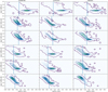 |
Fig. 1. Skew of the XID+ fluxes for all MIPS, PACS, and SPIRE bands in the three LOFAR deep fields. The contours show the density of the LOFAR sources whose multi-wavelength counterpart was originally undetected in the FIR. The histogram beneath the contours shows the distribution of all FIR sources in the LOFAR catalogues. The vertical lines show the flux below which a source’s posterior is dominated by the prior. |
The FIR fluxes that are available from HELP are at 24 (from Spitzer MIPS observations), 100, 160, 250, 350, and 500 μm (from Herschel PACS and SPIRE respectively, Pilbratt et al. 2010) which required two different prior lists for XID+, one for 24 μm and one for the longer wavelengths (due to the differences in resolution between MIPS and PACS + SPIRE). The prior list for 24 μm was constructed from a subset of the HELP masterlist. This was created by merging optical, NIR, and MIR catalogues that overlap with the Herschel observations, the details of which can be found in Shirley et al. (2019). This is necessary because if the 24 μm prior list were instead comprised of the entire HELP masterlist then XID+ would find a large degeneracy in the galaxy fluxes due to the high source density relative to the MIPS resolution. To remove this degeneracy, we exclude sources from the prior list that are expected to have a negligible 24 μm flux density. To this end, a number of cuts were applied to the merged catalogue to select sources that have significant emission at 24 μm. The prior list used for deblending the MIPS observations was constructed by only including objects detected by Spitzer (3.6−8.0 μm) and at shorter wavelengths. These cuts select objects most likely to be bright at 24 μm while removing artifacts from Spitzer. The PACS and SPIRE prior list was constructed by only considering objects from the 24 μm prior list whose 24 μm flux density was greater than the cutoff flux (Fig. 1; this is the same 24 μm flux density cut used to define the PACS and SPIRE prior list) as there is a correlation between flux at 24 μm and flux measured from PACS and SPIRE. A uniform flux prior was used for MIPS, PACS, and SPIRE.
For each galaxy, we can also examine the goodness of fit of the flux posterior. By looking at the flux distribution of a pixel, we can evaluate how likely we are to draw the measured pixel flux. If on average the pixels to which a given source is contributing are more than 2σ away from the true value then we flag that source as having an unreliable flux. This can be caused by missing a source from our prior list that is contributing to the map or because the included source does not contribute to the map.
Additional FIR bands were available from MIPS (70 and 160 μm) and PACS (70 μm) as well as 850 μm from SCUBA-2. However, the additional data from PACS and MIPS are of very low sensitivity and would therefore add very little value. The SCUBA-2 data typically probe higher redshift galaxies while LOFAR predominantly observes lower redshift star-forming galaxies. In addition, there are only several thousand galaxies detected in the SCUBA-2 Cosmology Legacy Survey (S2CLS; Geach et al. 2017) survey in Lockman-Hole and these can be cross-matched to the LOFAR catalogue by a simple nearest neighbour cross-match. This was done by Ramasawmy et al. (2021) and found only tens of matches, and so it has not been included in the data release.
2.4. Physical parameters and SED fitting
Photometric redshifts were measured for the full multi-wavelength catalogues using the method outlined in Duncan et al. (2021), which is briefly summarised here. By combining Gaussian processes and template fitting using a hierarchical Bayesian framework, photometric redshifts were estimated from multi-band photometry spanning from the near-ultraviolet (NUV) to NIR. The Gaussian processes were trained on galaxies with a spectroscopically confirmed redshift.
SEDs were computed for each radio source with a multi-wavelength cross-match using five different SED fitting codes: BAGPIPES (Carnall et al. 2019), MAGPHYS (Da Cunha et al. 2008), AGNFITTER (Calistro Rivera et al. 2016), and CIGALE using two different AGN models: namely those of Fritz et al. (2006) and Stalevski et al. (2016). A full comparison of the results of each of the SED-fitting codes is presented by Best et al. (in prep.). Here we give a brief description. Good agreement was found between all the codes for the stellar mass, SFR, and dust luminosity, with some small scatter, but no systematic offsets. The codes differ in their treatment of AGN; both BAGPIPES and MAGPHYS do not contain any AGN components in their models whereas AGNFITTER and CIGALE do. As a general rule, when there is no significant AGN activity in a galaxy, MAGPHYS and BAGPIPES obtain better fits than either AGNFITTER or CIGALE as with fewer parameters they are able to better explore their parameter space. On the other hand, MAGPHYS and BAGPIPES do not provide good fits for the majority of AGN, which are better fit by CIGALE and AGNFITTER. A comparison of the results of the different codes therefore allows identification of sources with AGN features; a full description of the AGN identification method is presented in Sect. 4.2.
3. Cross-matching
3.1. Radio to multi-wavelength
The radio sources were cross-matched to the multi-wavelength catalogue using a combination of likelihood ratio (LR) and manual cross-matching as described in Kondapally et al. (2021). Likelihood ratios are calculated using the formula from (Sutherland & Saunders 1992):
 (2)
(2)
where q(m, c) is the combined magnitude colour distribution of the true radio counterparts, n(m, c) is the normalised magnitude colour distribution of all multi-wavelength sources, and f(r) is the probability of the separation between the radio and multi-wavelength source.
Manual cross-matching was carried out for sources that were deemed unsuitable for LR cross-matching and were then visually inspected using the LOFAR galaxy zoo platform. Unsuitable sources included extended sources, sources with multiple Gaussian components, and clustered sources. Members of the LOFAR consortium inspected the optical/NIR postage stamps around the radio source overlaid with the radio contours and made their best interpretation in regards to the true multi-wavelength counterpart. Each radio galaxy was inspected by five different members and then if a consensus had been reached on the galaxy counterpart(s) then this was taken. If no clear consensus had been reached, then either the galaxy would not be assigned a counterpart, or it would be sent to an expert workflow where it was inspected in more detail. This choice depended on the reason for no consensus being reached and is discussed in full in Kondapally et al. (2021).
3.2. Far-infrared cross-matching
We used the following procedure to measure the FIR flux from the radio sources. First we cross-matched the LOFAR multi-wavelength counterparts with the HELP prior list using a search radius of 0.5″, which corresponds to the positional uncertainty of the Spitzer IRAC sources. If there is a source from the HELP prior list within 0.5″ then the FIR fluxes measured for that source were assigned to the radio counterpart. If the radio source has no multi-wavelength counterpart or there is no HELP prior list source within 0.5″ then XID+ is rerun around each of these sources using the same prior list as HELP but with the addition of the radio source (using the position of the multi-wavelength counterpart if there is one, otherwise the radio position is used) and a uniform flux prior is used. For the HELP XID+ run, the FIR maps were divided into tiles of equal area based on the HEALPIX tiling system, which were individually run through XID+. As the XID+ run for LOFAR uses circular regions (with a radius of 60″), because we did not need to rerun XID+ across the entire deep fields, we compared the fluxes we measured for the non-radio-galaxy counterparts to their fluxes measured in HELP. The results can be seen in Fig. 2 and show good agreement between the two measurements within their measured uncertainty (i.e. ≈60% of sources agree within one uncertainty). The results are symmetric about the x = y line apart from a subset of sources that are brighter in HELP than in the LOFAR run. These sources are all close to the new radio galaxy that was added to the prior list. We would expect them to be fainter in the LOFAR run as the flux in the map is being assigned to the radio source. In total we have FIR fluxes for 79 609 galaxies with detections at 150 MHz across the three deep fields.
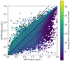 |
Fig. 2. Comparison between the flux measured with XID+ using the HELP and LOFAR prior lists. The colour shows the average distance from the LOFAR source for all sources in that bin (and hence the centre of the rerun region). We note the asymmetry about the x = y line on the right hand side of the plot where sources are brighter with the HELP prior compared to the LOFAR prior. This discrepancy is caused by the inclusion of the radio source in the LOFAR prior that causes sources in the HELP prior to have less flux assigned to them. The flux measurement from the LOFAR prior list is consistent with the measurement using the HELP prior list. |
4. Sample creation
4.1. Mass selection
To investigate how the FIRC depends on redshift and stellar mass we need to construct mass-complete samples, and we use the MAGPHYS SED fits from Smith et al. (2021) in ELAIS-N1 to construct these. Smith et al. (2021) used MAGPHYS to measure the SED for galaxies in the LOFAR catalogues with a 3.6 μm flux density > 10 μJy and estimated the completeness in stellar mass as a function of redshift using the method from Pozzetti et al. (2010). We created two samples using this information – one with z < 1.0 and M* > 1010.45, and the other with z < 0.4 and M* > 1010.05– to investigate the dependence of the FIRC on redshift and stellar mass, respectively (Fig. 3). We shall refer to these samples as the redshift sample and the mass sample.
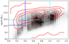 |
Fig. 3. Stellar mass–redshift distribution of the Smith et al. (2021) SED fits. The red contours show the distribution for galaxies with a detection at 150 MHz and the grey histogram shows the distribution for the galaxies without a detection at 150 MHz. The dark blue lines show the region selected for our mass sample and the light blue lines show the region selected for our redshift sample. |
MAGPHYS uses energy balance to match UV/optical and FIR templates so that the energy attenuated by dust in the UV/optical is equal to the energy radiated in the FIR. This energy balance allows an estimate of the TIR luminosity even when there are no individual FIR flux measurements, which ensures that all galaxies in our sample have a TIR luminosity measurement (Fig. A.1 shows the distribution of galaxies with less than one detection in SPIRE and PACS). The effect of using the energy balance approach when a galaxy has no individual detections from PACS or SPIRE is validated in Fig. A.1 to ensure that no systematic bias is introduced from the SED fitting. In addition, Małek et al. (2018) tested the use of energy balance in measuring TIR luminosities by measuring the TIR luminosity for galaxies when their FIR fluxes were included and excluded and found the results to be in good agreement. This analysis was carried out using CIGALE rather than magphys but the energy balance principle used in both SED fitters is the same and gives us confidence that there is no systematic bias in the TIR luminosity measurements for galaxies with no PACS or SPIRE fluxes.
Not all galaxies have a radio detection and therefore an upper limit on the radio flux is calculated (detailed in next paragraph). We then impose a cut on specific star formation rate (sSFR, SFR/M*) to select star-forming galaxies. For a galaxy to be considered as star forming, it must be no more than 0.6 dex below the main sequence (MS). We calculate the MS for each galaxy using Eq. (A.1) from Sargent et al. (2014) depending on its stellar mass and redshift. We use 0.6 dex as this corresponds to two standard deviations away from the MS (the effects of changing the offset from 0.6 dex are discussed in Sect. 6.1). This cut removes passive galaxies from our sample while not excluding starburst galaxies. Lacki et al. (2010) showed that starburst galaxies should theoretically lie along the FIRC and Magnelli et al. (2015) found this to be true in COSMOS. Therefore, we do not apply a cut above the SF main sequence. Table 2 shows how the different cuts reduce the number of galaxies in our sample (we also remove AGN from our sample and this is discussed in Sect. 4.2).
Number of galaxies in our sample after each cut is made.
For galaxies with a radio detection, we calculated their rest-frame luminosity at 150 MHz using
 (3)
(3)
where L150 is the rest-frame luminosity at 150 MHz, α is the radio spectral index, and S150 is the measured flux at 150 MHz. We take the spectral index to be −0.60 which is the spectral index measured between 150 MHz and 325 MHz in Calistro Rivera et al. (2017) which is appropriate to use for our sample of z < 1 galaxies as the highest rest frame frequency in our sample is 300 MHz. For the sources with no radio detection, we calculate a limit on their radio luminosity by taking the flux at 150 MHz to be 5σ, where σ is the rms noise in the pixel that contains the galaxy. This assumes that the undetected radio sources are spatially unresolved, which is valid due to the large angular resolution (6″) and is consistent with the threshold used to detect radio sources with PYBDSF (Tasse et al. 2021; Sabater et al. 2021).
4.2. AGN identification
The FIRC is believed to originate from radio and FIR emission linked to SF. The removal of AGN is essential for accurate measurement of this relation and its scatter. AGN can contribute to a galaxy’s SED in the IR and radio and thus could contaminate the FIRC.
Galaxies in our sample were identified as AGN if they were flagged as AGN in Duncan et al. (2021) – which includes AGN identified using their NIR colours following the criteria in Donley et al. (2012) –, had bright X-ray counterparts, were spectroscopically identified as AGN, or are part of the Million Quasar Catalog (Flesch 2019). In addition, Best et al. (in prep.) identified AGN in radio-detected sources (at 150 MHz) using the four different SED fits described in Sect. 2.4 as well as looking for evidence of excess radio emission based on the SFR–radio relation or extended radio emission. Finally, as part of selecting galaxies with a reliable MAGPHYS SED we excluded fits that had a poor χ2 (see Smith et al. 2012 for more details). Smith et al. (2021) found that 94% of galaxies flagged as AGN in Best et al. (in prep.) are also flagged by this method, and so we can be confident that AGN have been removed even if they are undetected in the radio.
5. Far-infrared radio correlation
We parameterise the FIRC using qTIR (the log ratio of the TIR to radio luminosity), defined as
 (4)
(4)
noting that LTIR is divided by the central frequency of 3.75 × 10¹² to make it dimensionless, and calculate qTIR for every galaxy in our sample. If a galaxy has an upper limit on its radio luminosity, then we calculate a lower limit of qTIR for that galaxy. We can then measure the median qTIR of our sample of galaxies using a survival analysis to account for the lower limits in qTIR. The survival analysis works by redistributing the lower limits assuming they follow the same underlying distribution, without making any assumptions as to the form of this distribution. This is implemented using the LIFELINES PYTHON package (Davidson-Pilon et al. 2021), which uses the Kaplan Meier estimator (Kaplan & Meier 1958), which in turn has had multiple applications within astronomy (Schmitt 1985). The median qTIR of our sample was measured by bootstrapping the survival analysis. This was done by repeating the measurement of the median using survival analysis 1000 times on a random 90% of our sample and the median measured for each of these samples. The median qTIR was taken as the mean of the distribution of medians from our bootstrapped samples and the error was taken as the standard deviation of the samples.
In the following sections, we describe how we validated our methodology by adding radio emission to the simulated IR dusty extragalactic sky (SIDES; Béthermin et al. 2017) simulation using a simple model. We then describe how the FIRC varies with different physical parameters.
5.1. SIDES FIRC simulation
To validate our methodology, we created a simulation of our samples using the SIDES simulation (Béthermin et al. 2017). SIDES simulates galaxies by generating their stellar mass from stellar mass functions. These galaxies are then matched to dark matter halos by abundance matching. Galaxies are then assigned to be either star forming or quiescent with the probability of a galaxy being star forming depending on its stellar mass and redshift. The FIR properties of the galaxies are then calculated based on their SFR; if a galaxy is quiescent then it has no FIR emission. It should be noted that AGN are not included in the SIDES simulation.
To ensure that our sample selection does not introduce any significant bias, we selected a mass-complete sample from the SIDES simulation using the same selection criteria as those used to create our real mass sample (i.e. M* > 1010.05 and z < 0.4) and removed galaxies based on their sSFR using the method described in Sect. 4.1. As the SIDES simulation does not include radio emission we created a simple model to add emission at 150 MHz to the SIDES galaxies that have log(M*) > 10.05 and z < 0.4. This was done by first giving each galaxy a qTIR value drawn from a Gaussian distribution with mean 1.8 and standard deviation 0.35. These parameters were chosen to provide a reasonable match to the qTIR distribution of the mass-complete sample. It should be noted that the distributions do not completely match and it is clear that the real qTIR distribution is not Gaussian. However, for the purposes of validating our method we do not need to perfectly reproduce our data. As we are measuring the median q we are unaffected by the small number of galaxies with low q values. As every galaxy has a qTIR value assigned to it, we can compute its radio luminosity and flux at 150 MHz and then determine whether or not it would be included in our radio catalogue (i.e. if S150 MHz > 0.1 mJy). If a galaxy would not have been detected then we computed the upper limit of its radio luminosity using Eq. (3) and taking the upper limit on its flux to be 0.1 mJy (0.1 mJy is the average 5σ rms noise) and then recalculated its qTIR using Eq. (4). We then performed a survival analysis on the simulated galaxies to measure the median of the ‘observed’ qTIR distribution, taking lower limits of qTIR into account, and found it to agree with the true median within the measured uncertainty (Fig. 4).
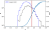 |
Fig. 4. Distribution of qTIR values from the SIDES simulation for galaxies with M* > 1010.45 and z < 1. The blue histogram is for lower limits of qTIR and the black histogram is for direct detections. The black vertical line (behind the dashed red line) marks the median of the sample, as measured using survival analysis and the red dashed vertical line shows the true median. The slight overestimation of the median is caused by the greater number of lower limits compared to direct detections. The blue line is the CDF of the entire sample, measured using survival analysis. |
We then modified our simple model to incorporate an evolution of qTIR with stellar mass. To do this, we set the mean of the Gaussian distribution used to draw qTIR to a function of stellar mass, μ = N(1 + M*)γ.
To investigate whether qTIR evolves with stellar mass, we divided our simulated galaxies into ten stellar mass bins such that the bins had an equal number of galaxies in them. The median qTIR in each bin was then measured using a survival analysis. We can then fit a power law of the form,
 (5)
(5)
with N and γ as free parameters. To measure the value of the free parameters, we bootstrapped our data by taking a random 90% of our data and fitting the power law to it using the method outlined above. We then took the value of the free parameters to be the median of the 1000 individual values measured, with an uncertainty equal to the standard deviation of the individual values. Using this method we were able to recover the intrinsic (measured by using all the radio luminosities rather than a combination of radio luminosities and upper limits for those with S150 MHz > 0.1 mJy) parameters of the power law within 1σ (Figs. 5 and 6). Therefore, if qTIR evolves with stellar mass in our LOFAR sample we are confident that we could recover the power-law parameters for that evolution.
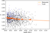 |
Fig. 5. Evolution of qTIR with M* for the SIDES simulation (M* > 1010.05 and z < 0.4) when qTIR is drawn from a Gaussian distribution whose mean is M* dependent. The orange points are the measured medians in their bins and the orange line is the fit to the medians. The red crosses and line are the true medians and fit; the red line is beneath the orange line. |
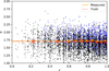 |
Fig. 6. Evolution of qTIR with redshift for the SIDES simulation (M* > 1010.45 and z < 1.0) when qTIR is drawn from a Gaussian distribution whose mean is M* dependent. The orange points are the measured medians in their bins and the orange line is the fit to the medians. The red crosses and line are the true medians and fit. |
Additionally, we are able to check whether a dependence of the FIRC on stellar mass would cause an observed evolution of the FIRC with redshift. We measured the evolution of qTIR with redshift for a simulated sample of galaxies whose qTIR varies with stellar mass. We found no observed evolution of qTIR with redshift in this scenario. This gives us confidence that if we observe evolution of qTIR with redshift in our redshift sample, then the evolution is genuine and not an artifact of any observed variation with stellar mass.
Finally, we investigated the case where we have more galaxies with upper limits on their radio luminosity than measurements. To change this, we artificially raised the flux limit (0.5 mJy for the mass sample and 0.25 for the redshift sample, which gives a ratio of detections to upper limits of ≃0.5) above which a galaxy is detectable at 150 MHz, and remeasured the evolution of qTIR with stellar mass and redshift. We found that having significantly more lower limits on q than direct detections does not cause a significant bias in our results. Even in the lowest mass bin, or highest redshift bin, respectively, where the ratio of detections to upper limits is less than 0.5. These simulations give us confidence that we can correctly measure the underlying parameters that describe the evolution of qTIR with both stellar mass and redshift.
5.2. FIRC with stellar mass and redshift
For our redshift sample we measured the median q = 1.879 ± 0.002 (Fig. 7) with typical uncertainties on individual measurements of q of 0.1 − 0.2 dex. We investigated the evolution of qTIR with redshift within our redshift sample using the method outlined in the previous section. By fitting a power law to measure the redshift evolution we can compare with the results of Delhaize et al. (2017) and Calistro Rivera et al. (2017). The fit parameters can be seen in Table 3 (we also fit a linear function). The results can be seen in Fig. 8 where we show how the median qTIR of our sample changes with redshift. The orange line shows our measured relation which shows a much shallower evolution compared to that found by Calistro Rivera et al. (2017) and Delhaize et al. (2017) (red and green lines, respectively). We also investigated the evolution of qTIR with stellar mass. This was done by repeating the above methodology with our mass sample to investigate how qTIR depends on stellar mass and the results can be seen in Fig. 9.
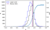 |
Fig. 7. Distribution of qTIR values for the redshift sample with M* > 1010.2 and z< 1. The black histogram is the qTIR distribution for galaxies that are detected at 150MHz. The blue histogram is the distribution of lower limits of qTIR for galaxies that have an upper limit at 150MHz and therefore their qTIR is a lower limit. The vertical line marks the median of the sample, as measured using survival analysis and the purple line shows the median qTIR from Molnár et al. (2021), measured at 1.4 GHz and converted to 150MHz using α = −0.78 |
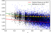 |
Fig. 8. Variation of the FIRC at 150 MHz with redshift for the redshift sample. The black points are direct detections in the radio and the blue points are undetected in the radio and are therefore lower limits in q. The orange points are the median qTIR measured using survival analysis in each redshift bin and the orange line is the power law fit to those points. The red line is the fit from Calistro Rivera et al. (2017) and the green line is the fit from Delhaize et al. (2017) converted to 150 MHz with a spectral index of −0.78. |
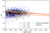 |
Fig. 9. Variation of the FIRC at 150 MHz with stellar mass for our mass sample. The blue points are upper limits of radio luminosity (lower limit on q) and the black points are for direct detections. The orange points are the median qTIR measured using survival analysis in each stellar mass bin and the orange line is the linear fit to those points. The light blue crosses are the median qTIR within each bin measured using the method described in Smith et al. (2021), while the yellow points are the median qTIRs measured with stacking. The red lines are the linear fit from Eq. (6) of Delvecchio et al. (2021) at the median redshift of our sample converted to 150 MHz with three spectral indices (see legend). |
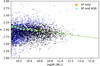 |
Fig. 10. Variation of the FIRC at 150 MHz with stellar mass for our mass sample. The blue points are upper limits of radio luminosity (lower limit on q) and the black points are for direct detections. The orange points are the median qTIR within each stellar mass bin measured using the survival analysis on only SF galaxies, and the orange line is a linear fit to these medians. The light blue crosses and line are the same but when AGN are included in the sample. We note how the blue crosses overlap with the orange points. |
Fit parameters for different samples.
Finally, we investigated the joint evolution of the FIRC with redshift and stellar mass using a sample of galaxies with z < 0.4 and M* > 1010.45 (giving 1171 galaxies detected at 150 MHz and 281 galaxies with upper limits on their flux at 150 MHz). The sample was split into four redshift bins with an equal number of galaxies in each bin and then each redshift bin is split into four stellar mass bins that all have an equal number of galaxies in them. We then fit the combined evolution using the method described above and find an evolution of the form qTIR(z, M*) = (1.98 ± 0.02)(1 + z)0.02 ± 0.04 + ( − 0.22 ± 0.03)log(M*)−10.45.
To further validate our results, we remeasured the median qTIR in our stellar mass bins using two alternative methods. Firstly, we employed the method from Smith et al. (2021). Briefly, in this method the PDF of the stellar mass versus qTIR plane is constructed by sampling from the radio flux posterior and TIR luminosity posterior of an individual galaxy. These posteriors, for galaxies detected at 150 MHz, are taken to be Gaussian distributions with mean equal to the measured value (for the TIR luminosity we used to 50th percentile output from magphys) and standard deviation equal to the error on that mean. For each posterior sample, we can calculate its radio luminosity and therefore its qTIR. The 150 MHz flux posterior for galaxies undetected at 150 MHz is taken to be a Gaussian with mean equal to the flux in the pixel where the galaxy is located, and standard deviation equal to the error of the flux in that pixel. Samples with a negative 150 MHz luminosity are set to the arbitrary limit of 1017 W Hz−1, and similarly, negative TIR luminosities are set to 106 L⊙. The samples are then summed in the stellar mass versus qTIR plane to measure the combined PDF. Within each of our stellar mass bins we can then measure the median qTIR from the combined PDF and compare it to the median qTIR measured using survival analysis (Fig. 9). The second method employed is stacking. Instead of measuring the upper limit of the flux at 150 MHz of each undetected radio galaxy, we measured the average flux at 150 MHz for all galaxies within the same stellar mass bin. This was done for all galaxies regardless of whether they were detected or not as the vast majority of our sample is unresolved at 150 MHz, and so the pixel flux is equal to the total flux. This was done by taking the mean of the fluxes in the pixels in which the undetected galaxies (undetected at 150 MHz) were located (we tested using the median flux instead of the mean and found the answers to be within one standard deviation of each other). This mean flux was converted into a radio luminosity using the mean redshift of those galaxies. The mean qTIR was similarly calculated using the mean TIR luminosity and the results can be seen in Fig. 9. We note that our crude stacking method does not account for any bias caused by galaxy clustering. Therefore, our stacked radio luminosities are likely higher than the true value, which would cause the median qTIR to be lower than the true value and could explain why stacking produces a systematically lower qTIR. The good agreement between all three methods give us further confidence that our method (survival analysis) is able to accurately measure the true evolution of our samples.
5.3. FIRC non-linearity
There has been little research done into whether the FIRC is non-linear at 150 MHz. Wang et al. (2019) found a sublinear relation between radio luminosity for a sample of low-redshift galaxies with high IR luminosities. To test whether the slope of the FIRC is 1, we binned the galaxies from our redshift sample (as this has more galaxies in it) into ten dust luminosity bins, spaced so that there is an equal number of galaxies in each bin. In each bin, we found the median qTIR using the method detailed in Sect. 5.2 and converted that median qTIR to a radio luminosity using Eq. (4) and taking LTIR to be at the centre of the bin. We then fit a linear relation to these data points of the form LTIR = β1 L150 MHz + β0 and found β1 = 0.90 ± 0.01, β0 = −9.8 ± 0.3 (Fig. 11). This shows a statistically significant deviation from a linear FIRC. However, due to the variation of qTIR with mass, it is difficult to disentangle the two relations and say whether the variation with mass causes the non-linearity or vice versa, as our sample is not complete in LTIR (we consider this in more detail below). Smith et al. (2021) found a non-linear relation between SFR and L150 (Eq. (1) in their paper) with slope 0.945 ± 0.07 (when substituting SFR with LTIR and converted to the same form as our relation). While the slopes are > 5σ apart, the difference can be attributed to the assumption that LTIR ∝ SFR. Any slight deviations from this assumption would cause a difference in the slopes between our work and that of Smith et al. (2021). In addition, we find a shallower slope than that observed by Wang et al. (2019) who found a slope of 0.77. However, their sample was constructed from IRAS-detected galaxies across the hetdex region (∼400 deg2) that by construction will be bright in the IR and have a median redshift of ∼0.05. It is hard to match their sample selection as we have few galaxies with such a low redshift because of the smaller area covered by the LoTSS observations in ELAIS-N1.
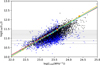 |
Fig. 11. Total-infrared luminosity (8 − 1000 μm) measured using MAGPHYS vs. radio luminosity at 150 MHz for all galaxies. The horizontal lines show the bins that the galaxies were divided into such that each bin contains an equal number of galaxies. The orange points are the median qTIR measured using survival analysis in each LTIR bin and the orange line is the linear fit to those points (we note that the orange points are often behind the cyan and red crosses). Blue data points are upper limits on radio luminosity and black points are direct detections at 150 MHz. The red line is the linear relation we would expect if our galaxies followed the main sequence measured by Schreiber et al. (2015) and the light blue line is that expected if they followed the main sequence measured by Leslie et al. (2020). |
6. Discussion
Here we present our results in the context of past studies (Sect. 6.1), how our sample selection and assumptions affect the observed variation of qTIR with stellar mass (Sect. 6.2), whether or not the FIRC being non-linear at 150 MHz is consistent with the main sequence (Sect. 5.3), and the causes for the dispersion around the FIRC (Sect. 6.4).
6.1. Comparison with past measurements
Our results have a similar normalisation to those of Delhaize et al. (2017) (study done in COSMOS at 1.4 GHz) but show a shallower evolution, which is likely caused by the observed evolution in stellar mass that results in galaxies with lower stellar masses having higher qTIR. The sample used by Delhaize et al. (2017) did not have a cut in stellar mass, and so they would expect to see higher qTIR values at low redshift, where low-mass galaxies are observable and conversely lower qTIR at high redshift. This would explain their apparently stronger evolution with redshift. Similarly, Calistro Rivera et al. (2017) did not use a mass-complete sample. This similarly biased their results towards lower qTIR values and explains the majority of the differences between our results and theirs. We can directly confirm this by modifying our sample to match the selections used in Calistro Rivera et al. (2017). To do so, we only included galaxies with a peak flux at 150 MHz > 0.6 mJy and then reran the analysis described in Sect. 5.2, with  ; the results are shown in Fig. 12. Using a radio-selected sample brings us into much better agreement with Calistro Rivera et al. (2017). In conclusion, the evolution in redshift observed in most other studies appears to be a result of their incomplete sample selection with respect to stellar mass.
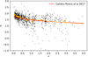 |
Fig. 12. Evolution of qTIR with redshift only using radio sources with peak flux > 0.6 mJy to mirror the sample selection of Calistro Rivera et al. (2017). We note the improved agreement between our fit (orange line) and the fit from Calistro Rivera et al. (2017) (red line) compared to using a mass-complete sample (Fig. 8). |
This contrasts with the results of Delvecchio et al. (2021) (Fig. 9), who used a mass-complete sample measured at 3 GHZ and then corrected to 1.4 GHZ with  , showing relatively little evolution with redshift but a clear dependency on stellar mass. These authors found good agreement between their sample and the results of Delhaize et al. (2017) when considering high-redshift galaxies. These are dominated by high-mass galaxies, and so the sample used in Delhaize et al. (2017) is close to the mass-complete one used in Delvecchio et al. (2021). Meanwhile, we found a steeper relation between qTIR and stellar mass and a higher normalisation than Delvecchio et al. (2021). Our tests with the SIDES simulation showed that our use of the survival analysis is able to accurately recover the true relation of our sample. So, unless some of the underlying assumptions used in our work are incorrect (such as choice of spectral index, which is examined in the following section) then we are confident that the differences are caused by the different frequencies used in our works. We expect to have a different ratio of thermal to synchrotron emission at the respective frequencies of our study and that of Delvecchio et al. (2021), and these differences could result in a different normalisation and slope.
Finally, Fig. 7 shows a reasonable agreement between the median qTIR of our redshift sample and that of Molnár et al. (2021). Their sample was constructed from low-redshift SDSS galaxies at 1.4 GHz, and so some differences are expected. We converted their median to 150 MHz using a spectral index of −0.73 and a higher spectral index would also explain the difference (see the following section for a more in-depth discussion on the choice of spectral index).
6.2. Mass evolution
Our results are based on several choices and assumptions made during our analysis and sample selection. Here we examine how changing those assumptions affects our results, focusing on: choice of spectral index, different FIR versus radio depths, removal of AGN, and selection of SF galaxies.
We used the spectral index measured in Calistro Rivera et al. (2017) of  , the mean of a Gaussian fitted to the observed distribution. Alternatively, we could have taken the mean of the distribution itself (−0.63), but Fig. 13 shows that the choice of spectral index makes little difference to the normalisation of our measured relation and no difference to the slope (solid lines). This is due to the small redshift range that our stellar mass sample was constructed in (z < 0.4), meaning that any correction to the rest frame frequency will be minor even at z = 0.4. However, when comparing to Delvecchio et al. (2021), the choice of
  has a big impact on the difference in normalisation between our results. We used
  as it is the mean of the
  distribution measured in Calistro Rivera et al. (2017). These latter authors also fit a Gaussian to the spectral index distribution with a mean of −0.73. Regardless, even if we use the higher spectral index we still find that their q1.4 = 2.53 becomes q150 = 1.82 which is still 0.2 dex below our results and can only explain 0.07 dex of the difference. Alternatively, Calistro Rivera et al. (2017) show
  as a function of redshift and find a large variation at low redshift, with results varying between −0.85 and −0.59 for z < 0.5. Taking the highest spectral index would put our results and those of Delvecchio et al. (2021) in good agreement (shown in Fig. 9). In addition, we investigated whether the different choices of spectral index used to convert to rest frame frequencies of 150 MHz and 1.4 GHz respectively could account for the difference. We converted their relation back to the observed frequency of 3 GHz using their assumed spectral index of −0.75 and then reconverted to 1.4 GHz. The subsequent conversion from 1.4 GHz to 150 MHz and converting our results from the observed frame to 150 MHz were all done with the same spectral index and the results can be seen in Fig. 13. This shows that the choice of spectral index only has a minor effect on the normalisation of our fit, which is to be expected due to the low redshift of our stellar mass sample. However, if the spectral index is closer to −0.6 then our normalisation would be in better agreement with that of Delvecchio et al. (2021). Overall, we are confident that varying
  within reasonable values has little to no impact on our measured relations but the choice of
  does greatly affect comparisons with work done at higher frequencies.
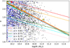 |
Fig. 13. Effect of different spectral indices on the linear fit of the FIRC with stellar mass and how our fits compare to those of Delvecchio et al. (2021). The solid lines show our relation depending on the choice of spectral index (see legend) and the dashed line shows the fit from Delvecchio et al. (2021) when converted to 150 MHz with the same spectral index. The black points show galaxies that are detected at 150 MHz and the blue points show galaxies that have upper limits on there flux at 150 MHz. |
Next we consider the difference in FIR versus radio depth. Our sample is created from an IRAC-selected sample and then limited to a mass-complete sample of star-forming galaxies. As the measurements of IR luminosity are done using MAGPHYS and an energy balance, there are many galaxies with a TIR luminosity measurement that are not detected in any individual FIR bands. This makes our sample deeper in the IR than the radio, in contrast to the sample used by Delvecchio et al. (2021) whose radio data were deeper than their IR data. We investigated whether this difference in depths could explain the measured discrepancy between our results. This was done by imposing a cut on the IR flux (calculated dividing the IR luminosity by  ) and then increasing this cut over a range of 2.0 dex. The greatest change in normalisation was ∼0.1 dex, obtained by imposing a harsh cut in our sample (Fig. 14) that has no physical motivation. In addition, such a harsh cut in TIR flux would likely be introducing significant bias towards lower qTIR values. Finally, it is worth emphasising that the maximum effect this can have on the normalisation of our linear fit is to decrease it by ∼0.1 dex which still leaves us with a significant disagreement with Delvecchio et al. (2021) when taking the nominal value of
  .
.
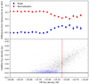 |
Fig. 14. Top: difference of linear fit parameters compared to Delvecchio et al. (2021) depending on the limit applied to the TIR flux. The red and blue points show the normalisation and slope of the linear fit, respectively, for all galaxies with a TIR flux density to the right of the point. It can be seen that imposing increasingly strict cuts on the TIR flux density does not cause any significant bias in our results and does not explain the difference between our fit and that of Delvecchio et al. (2021) until the TIR flux cut starts to significantly cut into our radio-detected galaxies. Bottom: TIR flux density calculated by dividing the TIR luminosity by |

We consider the impact that removing AGN has on our results. We remeasured the evolution of qTIR with stellar mass but with AGN host galaxies included in the sample (all AGN were re-added to the sample) to see how they affect our results (Fig. 10). We can see that the inclusion of AGN does not significantly affect our results. This is due to the fact that we are fitting to the median qTIR within each redshift or stellar mass bin and so we are not as affected by outliers or the relatively low fraction of AGN within our sample (< 10%). The galaxies with the lowest qTIR values are potentially unidentified radio-loud AGN or galaxies with a low dust mass (and therefore the TIR luminosity does not map the full SFR).
Finally, we investigated the impact of how we remove passive galaxies from our sample. Both our mass sample and redshift sample define a passive galaxy as one that is more than 0.6 dex below the main sequence. This offset below the main sequence was chosen to match ≃2σ where σ is the dispersion in the main sequence. However, choosing to set the offset between 0.3 and 0.9 dex would be equally justified. We investigated the effect that changing this offset has on our results and found that the slope and normalisation of the linear fit to qTIR(M*) vary by 0.02 and 0.01 respectively. The change in normalisation is the same as our uncertainty on the normalisation and the variation in slope is only marginally greater than our uncertainty. While varying our SF galaxy criteria does have a minor impact on the measured relation, the impact is similar to the random error of our measured distributions.
6.3. Main-sequence prediction of FIRC
The SFR of a galaxy is known to be correlated with its mass and this MS has been observed many times (Schreiber et al. 2015; Leslie et al. 2020). For a given galaxy in our redshift sample, we know its radio luminosity (or upper limit), mass, and redshift, and so we are able to calculate its predicted SFR using the MS relations measured in Schreiber et al. (2015) and Leslie et al. (2020) and therefore its TIR luminosity using the relation from Kennicutt (1998). We can then bin our galaxies on their predicted TIR luminosity so that there is an equal number of galaxies in each bin. In each bin, we can compute the median qTIR using a survival analysis and see how we would expect the slope of the FIRC to vary based purely on predictions from the MS relations. We can see from Fig. 11 that the predicted non-linearity is in agreement with our observed non-linearity. This could imply that the physics causing the observed non-linearity is the same that causes the MS. This in turn could help calibrate the SFR–radio luminosity relation. However, if the relation between SFR and stellar mass, which in turn causes a change in TIR luminosity, results in a change in the relation between radio and TIR luminosity, we would expect the radio luminosity to be similarly affected, but this does not seem to be the case. Resolving such issues is beyond the scope of this work. However, we hope to address such topics in the near future.
6.4. FIRC dispersion
A little-explored property of the FIRC is the cause for the dispersion. While the FIRC is surprisingly linear, with the standard deviation being 0.2, qTIR values still span a range of 1.5 dex when considering only the detected galaxies. Understanding what affects the deviation of a galaxy from the median qTIR can provide some insight into the underlying physics behind the FIRC. For high-mass galaxies, stellar mass does affect the median qTIR, and it could also affect the dispersion. These galaxies are most likely to have low-level AGN emission (Sabater et al. 2019) and a large low-mass stellar population. Either of these could boost the radio or FIR emission of the galaxy through mechanisms that are unrelated to SF. Other parameters that could affect where a galaxy lies on the FIRC are SFR and sSFR, as the mechanisms governing the FIRC may begin breaking down for starburst galaxies (though this was not observed by Magnelli et al. 2015 or predicted by Lacki et al. 2010). Finally, the steepness of the radio spectra is indicative of how recent the SF in a galaxy has occurred and may cause a galaxy to lie off the FIRC as the FIR and radio may be less sensitive to SF that has occurred more or less recently.
In order to investigate for this effect, we also included proxies for the angular and physical size of the galaxy. These were taken as the ratio of the total radio flux divided by the peak radio flux and as the difference in magnitude in the r band between 1−2, 1−3, and 1−6″. These proxies for angular size were converted to a measure of physical size by multiplying them by the distance to the galaxy. Finally, a proxy for gas surface density was created by dividing SFR by physical size as this is one of the key parameters used in Lacki et al. (2010). All of these parameters were fed into a neural network to predict the difference between a galaxy’s qTIR value and the median qTIR (Δq). We found that the neural network had no significant ability to predict Δq when compared to the intrinsic scatter of the Δq distribution.
The lack of predictive power of the neural network could be caused by several factors. Firstly, the parameters that govern the radio and FIR emission, such as magnetic field strength, are difficult to directly measure. Without a way to proxy these measurements, it is difficult to constrain exactly the qTIR value that a given galaxy should have. In addition, the measurements of SFR from MAGPHYS measure the combined SFR detected in the UV, optical, and FIR. If the measured SFR is imperfect because of the dust geometry of the galaxy, then the galaxy may lie off the FIRC.
Further work is required to explain the scatter in the FIRC. We are unable to accurately assess the error in LTIR caused by unusual dust geometry. In addition, we have no measure of the radio spectral index, which may explain a portion of the scatter.
If some of the SFR is unobscured, either due to lower-than-expected dust mass or the geometry of the galaxy, then the galaxy may not lie on the FIRC and we would be unable to measure this from the features we provided to the neural network.
7. Conclusions
In this work, we measured FIR fluxes for all radio sources in the LoTSS deep fields. These fluxes were then used to derive the FIRC at 150 MHz using data from LoTSS (Shimwell et al. 2019) and Herschel (Oliver et al. 2012) used in combination with a mass-complete sample (Kondapally et al. 2021; Duncan et al. 2021) of star-forming galaxies to measure the FIRC. The TIR luminosity is measured using MAGPHYS (Da Cunha et al. 2008), which uses energy balance to infer the IR luminosity when FIR fluxes are not measured, enabling IR luminosity measurements for all galaxies in our sample. To account for non-detections in the radio and FIR we use survival analysis and upper limits on the radio flux for galaxies that are undetected at 150 MHz. We investigate the evolution of qTIR with redshift and stellar mass and compare to the recent results from Delvecchio et al. (2021) using the JVLA. Our main results are listed below.
-
We measured fluxes at 24, 100, 160, 250, 350, and 500 μm for 79 609 galaxies across the LoTSS deep fields. In addition, we provide flags to identify sources whose flux is unreliable. The flags are based on the goodness of fit of the flux posterior to the map and whether it is dominated by the prior. The fluxes are available in the LOFAR deep fields data release (column descriptions can be found online1).
-
We validated our methods by creating a simple model based on galaxies created as part of the SIDES simulation (Béthermin et al. 2017). Radio luminosities were added to star-forming galaxies by generating qTIR values from a Gaussian distribution, whose mean evolved as a power law that mimicked the observed distribution from our mass-complete sample. We determined whether a galaxy would be detected in the radio or not. We found that we were able to recover the true distribution parameters (the true mean and power-law parameters) from the simple model when we had more detected galaxies then undetected galaxies (at 150 MHz).
-
The FIRC was measured at 150 MHz with a mass-complete sample of star-forming galaxies. We also examined the evolution of qTIR with redshift and stellar mass, finding a power-law relation for both, of the form q(z) = 1.94 ± 0.01(1 + z)−0.04 ± 0.01. Similarly the evolution with stellar mass was found to have a linear relation, of the form q(M*) = (2.00 ± 0.01)+(−0.22 ± 0.02)(log(M*)−10.05).
-
Comparing with previous results we found a significant difference between our evolution with stellar mass and that of Delvecchio et al. (2021). Neither our different treatment of AGN nor the different radio versus FIR depths can explain the difference. However, our choice of spectral index from Calistro Rivera et al. (2017) could affect our result as we used the median
 instead of
  which was observed at low redshift. More work is needed to better understand the radio spectra in order to know whether or not using a higher spectral index would explain the discrepancy between our results. We also observe a significant difference between our redshift evolution and that of Calistro Rivera et al. (2017). However, this can be explained by our different sample selections.
 -
We investigated the non-linearity of the FIRC at 150 MHz and found that LTIR(M*) = 0.90 ± 0.01 L150 − 9.8 ± 0.3. This relation is in good agreement with that found by Smith et al. (2021) in the SFR–radio luminosity plane and Molnár et al. (2021) at 1.4 GHz. In addition, the non-linearity observed agrees with predictions from the MS (Schreiber et al. 2015; Leslie et al. 2020). Future work is needed to explore whether both relations originate from the same physical processes.
Acknowledgments
We thank the anonymous referee for their useful comments and suggestions which have improved the content and presentation of the paper. I.M. acknowledges support from STFC via grant ST/R505146/1. S.O. and P.D.H. acknowledges support from the Science and Technology Facilities Council (grant number ST/T000473/1). M.T.S. acknowledges support from a Scientific Exchanges visitor fellowship (IZSEZO_202357) from the Swiss National Science Foundation. K.M. is supported by the Polish National Science Centre grant UMO-2018/30/E/ST9/00082. R.K. acknowledges support from the Science and Technology Facilities Council (STFC) through an STFC studentship via grant ST/R504737/1. I.P. acknowledges support from INAF under the SKA/CTA PRIN “FORECaST” and the PRIN MAIN STREAM “SAuROS” projects. MB acknowledges support from INAF under the SKA/CTA PRIN “FORECaST” and the PRIN MAIN STREAM “SAuROS” projects and from the Ministero degli Affari Esteri e della Cooperazione Internazionale – Direzione Generale per la Promozione del Sistema Paese Progetto di Grande Rilevanza ZA18GR02. R.K.C. is grateful for the support of the John Harvard Distinguished Science Fellowship. J.S. is grateful for support from the UK STFC via grant ST/R000972/1. This paper is based (in part) on data obtained with the International LOFAR Telescope (ILT) under project codes LC0_015, LC2_024, LC2_038, LC3_008, LC4_008, LC4_034 and LT10_01. LOFAR (Van Haarlem et al. 2013) is the Low Frequency Array designed and constructed by ASTRON. It has observing, data processing, and data storage facilities in several countries, which are owned by various parties (each with their own funding sources), and which are collectively operated by the ILT foundation under a joint scientific policy. The ILT resources have benefitted from the following recent major funding sources: CNRS-INSU, Observatoire de Paris and Université d’Orléans, France; BMBF, MIWF-NRW, MPG, Germany; Science Foundation Ireland (SFI), Department of Business, Enterprise and Innovation (DBEI), Ireland; NWO, The Netherlands; The Science and Technology Facilities Council, UK; Ministry of Science and Higher Education, Poland.
References
- Bell, E. F. 2003, ApJ, 586, 794 [Google Scholar]
- Berta, S., Lutz, D., Santini, P., et al. 2013, A&A, 551, A100 [NASA ADS] [CrossRef] [EDP Sciences] [Google Scholar]
- Bertin, E. 1996, A&AS, 117, 393 [NASA ADS] [CrossRef] [EDP Sciences] [Google Scholar]
- Béthermin, M., Wu, H. Y., Lagache, G., et al. 2017, A&A, 607, A89 [NASA ADS] [CrossRef] [EDP Sciences] [Google Scholar]
- Brown, M. J. I., Dey, A., Jannuzi, B. T., et al. 2007, ApJ, 654, 858 [Google Scholar]
- Brown, M. J. I., Zheng, Z., White, M., et al. 2008, ApJ, 682, 937 [Google Scholar]
- Calistro Rivera, G., Lusso, E., Hennawi, J. F., & Hogg, D. W. 2016, ApJ, 833, 98 [Google Scholar]
- Calistro Rivera, G., Williams, W. L., Hardcastle, M. J., et al. 2017, MNRAS, 469, 3468 [Google Scholar]
- Carnall, A. C., Leja, J., Johnson, B. D., et al. 2019, ApJ, 873, 44 [Google Scholar]
- Casey, C. M., Narayanan, D., & Cooray, A. 2014, Phys. Rep., 541, 45 [Google Scholar]
- Condon, J. 1992, ARA&A, 30, 575 [Google Scholar]
- Da Cunha, E., Charlot, S., & Elbaz, D. 2008, MNRAS, 388, 1595 [NASA ADS] [CrossRef] [Google Scholar]
- Davidson-Pilon, C., Kalderstam, J., Jacobson, N., et al. 2021, https://doi.org/10.5281/zenodo.4579431 [Google Scholar]
- Davies, L. J. M., Huynh, M. T., Hopkins, A. M., et al. 2017, MNRAS, 466, 2312 [Google Scholar]
- Del Moro, A., Alexander, D. M., Mullaney, J. R., et al. 2013, A&A, 549, A59 [NASA ADS] [CrossRef] [EDP Sciences] [Google Scholar]
- Delhaize, J., Smolčić, V., Delvecchio, I., et al. 2017, A&A, 602, A4 [NASA ADS] [CrossRef] [EDP Sciences] [Google Scholar]
- Delvecchio, I., Daddi, E., Sargent, M. T., et al. 2021, A&A, 647, A25 [Google Scholar]
- Donley, J. L., Koekemoer, A. M., Brusa, M., et al. 2012, ApJ, 748, 142 [Google Scholar]
- Duncan, K. J., Kondapally, R., Brown, M. J. I., et al. 2021, A&A, 648, A21 [Google Scholar]
- Flesch, E. W. 2019, ArXiv e-prints [arXiv:1912.05614] [Google Scholar]
- Fritz, J., Franceschini, A., & Hatziminaoglou, E. 2006, MNRAS, 366, 767 [Google Scholar]
- Geach, J. E., Dunlop, J. S., Halpern, M., et al. 2017, MNRAS, 465, 1789 [Google Scholar]
- Griffin, M. J., Abergel, A., Abreu, A., et al. 2010, A&A, 518, L3 [EDP Sciences] [Google Scholar]
- Gruppioni, C., Pozzi, F., Rodighiero, G., et al. 2013, MNRAS, 432, 23 [Google Scholar]
- Gurkan, G., Hardcastle, M. J., Smith, D. J. B., et al. 2018, MNRAS, 475, 3010 [Google Scholar]
- Heesen, V., Buie, E., Huff, C. J., et al. 2019, A&A, 622, A8 [NASA ADS] [CrossRef] [EDP Sciences] [Google Scholar]
- Helou, G., & Bicay, M. D. 2002, ApJ, 415, 93 [Google Scholar]
- Hurley, P. D., Oliver, S., Betancourt, M., et al. 2017, MNRAS, 464, 885 [Google Scholar]
- Kaplan, E. L., & Meier, P. 1958, J. Am. Stat. Assoc., 53, 457 [Google Scholar]
- Kennicutt, R. C., Jr. 1998, ApJ, 498, 541 [Google Scholar]
- Kondapally, R., Best, P. N., Hardcastle, M. J., et al. 2021, A&A, 648, A104 [NASA ADS] [CrossRef] [EDP Sciences] [Google Scholar]
- Lacki, B. C., Thompson, T. A., & Quataert, E. 2010, ApJ, 717, 1 [Google Scholar]
- Leslie, S. K., Schinnerer, E., Liu, D., et al. 2020, ApJ, 899, 58 [Google Scholar]
- Magnelli, B., Ivison, R. J., Lutz, D., et al. 2015, A&A, 573, A45 [NASA ADS] [CrossRef] [EDP Sciences] [Google Scholar]
- Małek, K., Buat, V., Roehlly, Y., et al. 2018, A&A, 620, A50 [Google Scholar]
- Mandal, S., Prandoni, I., Hardcastle, M. J., et al. 2021, A&A, 648, A5 [EDP Sciences] [Google Scholar]
- Molnár, D. C., Sargent, M. T., Delhaize, J., et al. 2018, MNRAS, 475, 827 [Google Scholar]
- Molnár, D. C., Sargent, M. T., Leslie, S., et al. 2021, MNRAS, 504, 118 [CrossRef] [Google Scholar]
- Murphy, E. J. 2009, ApJ, 706, 482 [Google Scholar]
- Oliver, S. J., Bock, J., Altieri, B., et al. 2012, MNRAS, 424, 1614 [NASA ADS] [CrossRef] [Google Scholar]
- Pilbratt, G. L., Riedinger, J. R., Passvogel, T., et al. 2010, A&A, 518, L1 [NASA ADS] [CrossRef] [EDP Sciences] [Google Scholar]
- Poglitsch, A., Waelkens, C., Geis, N., et al. 2010, A&A, 518, L2 [NASA ADS] [CrossRef] [EDP Sciences] [Google Scholar]
- Pozzetti, L., Bolzonella, M., Zucca, E., et al. 2010, A&A, 523, A13 [NASA ADS] [CrossRef] [EDP Sciences] [Google Scholar]
- Ramasawmy, J., Geach, J. E., Hardcastle, M. J., et al. 2021, A&A, 648, A14 [NASA ADS] [CrossRef] [EDP Sciences] [Google Scholar]
- Read, S. C., Smith, D. J., Gürkan, G., et al. 2018, MNRAS, 480, 5625 [CrossRef] [Google Scholar]
- Rieke, G. H., Young, E. T., Engelbracht, C. W., et al. 2004, ApJS, 154, 25 [Google Scholar]
- Sabater, J., Best, P. N., Hardcastle, M. J., et al. 2019, A&A, 622, A17 [NASA ADS] [CrossRef] [EDP Sciences] [Google Scholar]
- Sabater, J., Best, P. N., Tasse, C., et al. 2021, A&A, 648, A2 [EDP Sciences] [Google Scholar]
- Safarzadeh, M., Ferguson, H. C., Lu, Y., Inami, H., & Somerville, R. S. 2014, ApJ, 798, 91 [CrossRef] [Google Scholar]
- Sargent, M. T., Schinnerer, E., Murphy, E., et al. 2010, ApJ, 714, 190 [Google Scholar]
- Sargent, M. T., Daddi, E., Béthermin, M., et al. 2014, ApJ, 793, 19 [NASA ADS] [CrossRef] [Google Scholar]
- Schmitt, J. H. M. M. 1985, ApJ, 293, 178 [NASA ADS] [CrossRef] [Google Scholar]
- Schreiber, C., Pannella, M., Elbaz, D., et al. 2015, A&A, 575, A74 [NASA ADS] [CrossRef] [EDP Sciences] [Google Scholar]
- Shimwell, T. W., Röttgering, H. J., Best, P. N., et al. 2017, A&A, 598, A104 [NASA ADS] [CrossRef] [EDP Sciences] [Google Scholar]
- Shimwell, T. W., Tasse, C., Hardcastle, M. J., et al. 2019, A&A, 622, A1 [NASA ADS] [CrossRef] [EDP Sciences] [Google Scholar]
- Shirley, R., Roehlly, Y., Hurley, P. D., et al. 2019, MNRAS, 490, 634 [Google Scholar]
- Smith, D. J., Dunne, L., da Cunha, E., et al. 2012, MNRAS, 427, 703 [NASA ADS] [CrossRef] [Google Scholar]
- Smith, D. J., Jarvis, M. J., Hardcastle, M. J., et al. 2014, MNRAS, 445, 2232 [NASA ADS] [CrossRef] [Google Scholar]
- Smith, D. J. B., Haskell, P., Gürkan, G., et al. 2021, A&A, 648, A6 [EDP Sciences] [Google Scholar]
- Smolčić, V., Novak, M., Delvecchio, I., et al. 2017, A&A, 602, A6 [NASA ADS] [CrossRef] [EDP Sciences] [Google Scholar]
- Stalevski, M., Ricci, C., Ueda, Y., et al. 2016, MNRAS, 458, 2288 [Google Scholar]
- Sutherland, W., & Saunders, W. 1992, MNRAS, 259, 413 [Google Scholar]
- Szalay, A. S., Connolly, A. J., Szokoly, G. P. 1999, AJ, 117, 68 [NASA ADS] [CrossRef] [Google Scholar]
- Tasse, C., Shimwell, T., Hardcastle, M. J., et al. 2021, A&A, 648, A1 [EDP Sciences] [Google Scholar]
- Terzian, Y. 1972, Symp. Int. Astron. Union, 44, 75 [NASA ADS] [CrossRef] [Google Scholar]
- Vaccari, M., & Consortium, T. H. 2015, HELP: The Herschel Extragalactic Legacy Project and The Coming of Age of Multi-Wavelength Astrophysics, Tech. Rep. [Google Scholar]
- Van der Kruit, P. C. 1971, A&A, 15, 110 [Google Scholar]
- Van Haarlem, M. P., Wise, M. W., Gunst, A. W., et al. 2013, A&A, 556, A2 [NASA ADS] [CrossRef] [EDP Sciences] [Google Scholar]
- Voelk, H. J. 1989, A&A, 218, 67 [NASA ADS] [Google Scholar]
- Wang, L., Gao, F., Duncan, K. J., et al. 2019, A&A, 631, A109 [NASA ADS] [CrossRef] [EDP Sciences] [Google Scholar]
- Yun, M. S., Reddy, N. A., & Condon, J. J. 2002, ApJ, 554, 803 [Google Scholar]
Appendix A: Energy balance assumption
Using the SED fits from Smith et al. (2021) we are relying on the energy balance approach used by magphys when there are no PACS or SPIRE fluxes to help constrain the FIR. Firstly, Figure A.1 shows that no part of the parameter space is dominated by galaxies that are dependant on the energy balance, and so the affect of any systematic bias, if any exists, would be minimal. As a second check we can compare the νLν at 24μm with the SFR measured from magphys. νLν at 24μm is a tracer of SF Rieke et al. (2004) and so by comparing their ratio for different subsamples we can see whether there are any significant deviations in this ratio between the subsamples. To calculate νLν at 24μm we k-corrected the measured Lν using the red galaxy template from Berta et al. (2013). Figure A.2 shows the comparison between galaxies with one or less detection from PACS or SPIRE compared to galaxies with more than one detection. We can see that the peak of both distributions are within ≃0.2 dex of each other, lending further evidence that relying on the energy balance from magphys does not cause a bias in measurements of SFR (and hence TIR luminosity as the two are tightly correlated). The small offset is likely caused by a poor choice of SED template for the k-correction. The subsample with few FIR detections is more likely to be populated by fainter galaxies or those at higher redshift and a different template may be needed to accurately measure their νLν at 24μm.
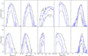 |
Fig. A.1. How galaxies are distributed, split by their observed fluxes and which sample they are in. The black line shows how the galaxies that are detected at 150 MHz are distributed and the blue line is for galaxies undetected at 150 MHz. If the line is dotted then it shows galaxies that have one unflagged (see section 2.3) flux from PACS or SPIRE and if solid then it has more than one unflagged flux from PACS or SPIRE. We can see that no part of the parameter space is dominated by galaxies that have one or less unflagged flux in PACS or SPIRE. |
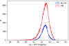 |
Fig. A.2. Comparison of νLν/SFR measured from magphys for the 3.6μm-selected sample in ELAIS-N1. The blue histogram shows the results for galaxies with one or less unflagged flux from PACS or SPIRE while the red histogram shows the results for galaxies with more than one unflagged flux from PACS or SPIRE. |
All Tables
All Figures
|
Fig. 1. Skew of the XID+ fluxes for all MIPS, PACS, and SPIRE bands in the three LOFAR deep fields. The contours show the density of the LOFAR sources whose multi-wavelength counterpart was originally undetected in the FIR. The histogram beneath the contours shows the distribution of all FIR sources in the LOFAR catalogues. The vertical lines show the flux below which a source’s posterior is dominated by the prior. |
| In the text | |
|
Fig. 2. Comparison between the flux measured with XID+ using the HELP and LOFAR prior lists. The colour shows the average distance from the LOFAR source for all sources in that bin (and hence the centre of the rerun region). We note the asymmetry about the x = y line on the right hand side of the plot where sources are brighter with the HELP prior compared to the LOFAR prior. This discrepancy is caused by the inclusion of the radio source in the LOFAR prior that causes sources in the HELP prior to have less flux assigned to them. The flux measurement from the LOFAR prior list is consistent with the measurement using the HELP prior list. |
| In the text | |
|
Fig. 3. Stellar mass–redshift distribution of the Smith et al. (2021) SED fits. The red contours show the distribution for galaxies with a detection at 150 MHz and the grey histogram shows the distribution for the galaxies without a detection at 150 MHz. The dark blue lines show the region selected for our mass sample and the light blue lines show the region selected for our redshift sample. |
| In the text | |
|
Fig. 4. Distribution of qTIR values from the SIDES simulation for galaxies with M* > 1010.45 and z < 1. The blue histogram is for lower limits of qTIR and the black histogram is for direct detections. The black vertical line (behind the dashed red line) marks the median of the sample, as measured using survival analysis and the red dashed vertical line shows the true median. The slight overestimation of the median is caused by the greater number of lower limits compared to direct detections. The blue line is the CDF of the entire sample, measured using survival analysis. |
| In the text | |
|
Fig. 5. Evolution of qTIR with M* for the SIDES simulation (M* > 1010.05 and z < 0.4) when qTIR is drawn from a Gaussian distribution whose mean is M* dependent. The orange points are the measured medians in their bins and the orange line is the fit to the medians. The red crosses and line are the true medians and fit; the red line is beneath the orange line. |
| In the text | |
|
Fig. 6. Evolution of qTIR with redshift for the SIDES simulation (M* > 1010.45 and z < 1.0) when qTIR is drawn from a Gaussian distribution whose mean is M* dependent. The orange points are the measured medians in their bins and the orange line is the fit to the medians. The red crosses and line are the true medians and fit. |
| In the text | |
|
Fig. 7. Distribution of qTIR values for the redshift sample with M* > 1010.2 and z< 1. The black histogram is the qTIR distribution for galaxies that are detected at 150MHz. The blue histogram is the distribution of lower limits of qTIR for galaxies that have an upper limit at 150MHz and therefore their qTIR is a lower limit. The vertical line marks the median of the sample, as measured using survival analysis and the purple line shows the median qTIR from Molnár et al. (2021), measured at 1.4 GHz and converted to 150MHz using α = −0.78 |
| In the text | |
|
Fig. 8. Variation of the FIRC at 150 MHz with redshift for the redshift sample. The black points are direct detections in the radio and the blue points are undetected in the radio and are therefore lower limits in q. The orange points are the median qTIR measured using survival analysis in each redshift bin and the orange line is the power law fit to those points. The red line is the fit from Calistro Rivera et al. (2017) and the green line is the fit from Delhaize et al. (2017) converted to 150 MHz with a spectral index of −0.78. |
| In the text | |
|
Fig. 9. Variation of the FIRC at 150 MHz with stellar mass for our mass sample. The blue points are upper limits of radio luminosity (lower limit on q) and the black points are for direct detections. The orange points are the median qTIR measured using survival analysis in each stellar mass bin and the orange line is the linear fit to those points. The light blue crosses are the median qTIR within each bin measured using the method described in Smith et al. (2021), while the yellow points are the median qTIRs measured with stacking. The red lines are the linear fit from Eq. (6) of Delvecchio et al. (2021) at the median redshift of our sample converted to 150 MHz with three spectral indices (see legend). |
| In the text | |
|
Fig. 10. Variation of the FIRC at 150 MHz with stellar mass for our mass sample. The blue points are upper limits of radio luminosity (lower limit on q) and the black points are for direct detections. The orange points are the median qTIR within each stellar mass bin measured using the survival analysis on only SF galaxies, and the orange line is a linear fit to these medians. The light blue crosses and line are the same but when AGN are included in the sample. We note how the blue crosses overlap with the orange points. |
| In the text | |
|
Fig. 11. Total-infrared luminosity (8 − 1000 μm) measured using MAGPHYS vs. radio luminosity at 150 MHz for all galaxies. The horizontal lines show the bins that the galaxies were divided into such that each bin contains an equal number of galaxies. The orange points are the median qTIR measured using survival analysis in each LTIR bin and the orange line is the linear fit to those points (we note that the orange points are often behind the cyan and red crosses). Blue data points are upper limits on radio luminosity and black points are direct detections at 150 MHz. The red line is the linear relation we would expect if our galaxies followed the main sequence measured by Schreiber et al. (2015) and the light blue line is that expected if they followed the main sequence measured by Leslie et al. (2020). |
| In the text | |
|
Fig. 12. Evolution of qTIR with redshift only using radio sources with peak flux > 0.6 mJy to mirror the sample selection of Calistro Rivera et al. (2017). We note the improved agreement between our fit (orange line) and the fit from Calistro Rivera et al. (2017) (red line) compared to using a mass-complete sample (Fig. 8). |
| In the text | |
|
Fig. 13. Effect of different spectral indices on the linear fit of the FIRC with stellar mass and how our fits compare to those of Delvecchio et al. (2021). The solid lines show our relation depending on the choice of spectral index (see legend) and the dashed line shows the fit from Delvecchio et al. (2021) when converted to 150 MHz with the same spectral index. The black points show galaxies that are detected at 150 MHz and the blue points show galaxies that have upper limits on there flux at 150 MHz. |
| In the text | |
|
Fig. 14. Top: difference of linear fit parameters compared to Delvecchio et al. (2021) depending on the limit applied to the TIR flux. The red and blue points show the normalisation and slope of the linear fit, respectively, for all galaxies with a TIR flux density to the right of the point. It can be seen that imposing increasingly strict cuts on the TIR flux density does not cause any significant bias in our results and does not explain the difference between our fit and that of Delvecchio et al. (2021) until the TIR flux cut starts to significantly cut into our radio-detected galaxies. Bottom: TIR flux density calculated by dividing the TIR luminosity by |
| In the text | |
|
Fig. A.1. How galaxies are distributed, split by their observed fluxes and which sample they are in. The black line shows how the galaxies that are detected at 150 MHz are distributed and the blue line is for galaxies undetected at 150 MHz. If the line is dotted then it shows galaxies that have one unflagged (see section 2.3) flux from PACS or SPIRE and if solid then it has more than one unflagged flux from PACS or SPIRE. We can see that no part of the parameter space is dominated by galaxies that have one or less unflagged flux in PACS or SPIRE. |
| In the text | |
|
Fig. A.2. Comparison of νLν/SFR measured from magphys for the 3.6μm-selected sample in ELAIS-N1. The blue histogram shows the results for galaxies with one or less unflagged flux from PACS or SPIRE while the red histogram shows the results for galaxies with more than one unflagged flux from PACS or SPIRE. |
| In the text | |
Current usage metrics show cumulative count of Article Views (full-text article views including HTML views, PDF and ePub downloads, according to the available data) and Abstracts Views on Vision4Press platform.
Data correspond to usage on the plateform after 2015. The current usage metrics is available 48-96 hours after online publication and is updated daily on week days.
Initial download of the metrics may take a while.