| Issue |
A&A
Volume 667, November 2022
|
|
|---|---|---|
| Article Number | A30 | |
| Number of page(s) | 30 | |
| Section | Extragalactic astronomy | |
| DOI | https://doi.org/10.1051/0004-6361/202142877 | |
| Published online | 01 November 2022 | |
Deciphering the radio–star formation correlation on kpc scales
II. The integrated infrared–radio continuum and star formation–radio continuum correlations
1
Université de Strasbourg, CNRS, Observatoire Astronomique de Strasbourg, UMR 7550, 67000 Strasbourg, France
e-mail: This email address is being protected from spambots. You need JavaScript enabled to view it.
2
Astronomical Observatory, Jagiellonian University, Kraków, Poland
Received:
10
December
2021
Accepted:
13
July
2022
Abstract
Given the multiple energy-loss mechanisms of cosmic-ray (CR) electrons in galaxies, the tightness of the infrared (IR)–radio continuum correlation is surprising. As the radio continuum emission at GHz frequencies is optically thin, this offers the opportunity to obtain unbiased star formation rates (SFRs) from radio-continuum flux-density measurements. The calorimeter theory can naturally explain the tightness of the far-infrared (FIR)–radio correlation but makes predictions that do not agree with observations. Noncalorimeter models often have to involve a conspiracy to maintain the tightness of the FIR–radio correlation. We extended a published analytical model of galactic disks by including a simplified prescription for the synchrotron emissivity. The galactic gas disks of local spiral galaxies, low-z starburst galaxies, high-z main sequence star-forming galaxies, and high-z starburst galaxies are treated as turbulent clumpy accretion disks. The magnetic field strength is determined by the equipartition between the turbulent kinetic and the magnetic energy densities. Our fiducial model, which includes neither galactic winds nor CR electron secondaries, reproduces the observed radio continuum spectral energy distributions of most (∼70%) of the galaxies. Except for the local spiral galaxies, fast galactic winds can potentially make the conflicting models agree with observations. The observed IR–radio correlations are reproduced by the model within 2σ of the joint uncertainty of model and data for all datasets. The model agrees with the observed SFR–radio correlations within ∼4σ. Energy equipartition between the CR particles and the magnetic field only approximately holds in our models of main sequence star-forming galaxies. If a CR electron calorimeter is assumed, the slope of the IR–radio correlation flattens significantly. Inverse Compton losses are not dominant in the starburst galaxies because in these galaxies not only the gas density but also the turbulent velocity dispersion is higher than in normal star-forming galaxies. Equipartition between the turbulent kinetic and magnetic field energy densities then leads to very high magnetic field strengths and very short synchrotron timescales. The exponents of our model SFR–radio correlations at 150 MHz and 1.4 GHz are very close to one.
Key words: galaxies: ISM / galaxies: magnetic fields / galaxies: star formation / radio continuum: galaxies
© B. Vollmer et al. 2022
 Open Access article, published by EDP Sciences, under the terms of the Creative Commons Attribution License (https://creativecommons.org/licenses/by/4.0), which permits unrestricted use, distribution, and reproduction in any medium, provided the original work is properly cited.
This article is published in open access under the Subscribe-to-Open model. This email address is being protected from spambots. You need JavaScript enabled to view it. to support open access publication.
1. Introduction
One of the tightest correlations in astronomy is the relation between the integrated radio continuum (synchrotron) and the far-infrared (FIR) emission (Helou et al. 1985; Condon 1992; Mauch & Sadler 2007; Yun et al. 2001; Bell 2003; Farrah et al. 2003; Appleton et al. 2004; Kovács et al. 2006; Murphy 2009; Sargent et al. 2010; Jarvis et al. 2010; Basu et al. 2015; Magnelli et al. 2015; Delhaize et al. 2017; Read et al. 2018; Thomson et al. 2019; Algera et al. 2020; Molnár et al. 2021; Delvecchio et al. 2021). This relation holds over five orders of magnitude in various types of galaxies, including starbursts. The common interpretation of the correlation is that both emission types are proportional to star formation: the radio emission via (i) the cosmic ray (CR) source term caused by supernova explosions and the turbulent amplification of the small-scale magnetic field (small-scale dynamo e.g., Schleicher & Beck 2013) and (ii) the FIR emission via the dust heating, mainly through massive stars.
In local galaxies, the correlation between the star formation rate (SFR) and the radio continuum emission is as tight as the correlation involving the FIR emission (Bell 2003; Murphy et al. 2011; Heesen et al. 2014, 2019; Boselli et al. 2015; Li et al. 2016; Brown et al. 2017; Gürkan et al. 2018; Wang et al. 2019; Smith et al. 2021). As the radio continuum emission at GHz frequencies is optically thin, this offers the opportunity to obtain unbiased SFRs from radio continuum flux density measurements (e.g., Davies et al. 2017). The possible contribution of an active galactic nucleus (AGN) has to be recognized and subtracted, if possible. Whereas the exponents – which are close to unity – and normalizations of the FIR– and star formation–radio continuum correlations are well studied, the detailed physics that lead to these relations are not thoroughly understood.
Radio continuum emission observed at frequencies below a few GHz is usually dominated by synchrotron emission, which is emitted by CR electrons with relativistic velocities that spiral around galactic magnetic fields. The magnetic field can be regular, meaning structured on large scales (kpc), or tangled on small scales via turbulent motions. The turbulent magnetic field has an isotropic and an anisotropic component. The total magnetic field B is the quadratic sum of the ordered and turbulent magnetic field components. The ordered magnetic field includes the large-scale regular magnetic field, and the anisotropic small-scale magnetic field. Anisotropic small-scale magnetic fields can be produced by a large-scale gas and associated magnetic field compression.
The energy loss caused by synchrotron emission depends on the magnetic field strength and the electron energy or Lorentz factor γ:
 (1)
(1)
where B = 10 μG is the typical magnetic field strength in local spiral galaxies (e.g., Beck 2015). A CR electron with energy E emits most of its energy at a critical frequency νc where
 (2)
(2)
where α is the pitch angle of the particle’s path with respect to the magnetic field direction. The timescale for synchrotron emission is
 (3)
(3)
For the calculation of the mean energy of CR electrons, we use the mean frequency calculated via the expectation value of x = ν/νc, where
 (4)
(4)
with the synchrotron kernel G(x) given by Eq. (D.3) of Aharonian et al. (2010). This yields
 (5)
(5)
Cosmic-ray particles are mainly produced in supernova shocks via Fermi acceleration. However, the relativistic electrons do not stay at the location of their creation. They propagate either via diffusion, or by streaming with the Alfvén velocity. In addition, CR electrons can be transported into the halo by advection, meaning a galactic wind. During the transport process, the CR electron loses energy via synchrotron emission. The associated diffusion–advection–loss equation for the CR electron density n reads as
 (6)
(6)
where D is the diffusion coefficient, E the CR electron energy, u the advective flow velocity, v the streaming velocity, p the CR electron pressure, Q the source term, and b(E) the rate of energy loss. The first part of the right-hand side of Eq. (6) is the diffusion term, followed by the synchrotron loss, advection, streaming, adiabatic energy gain or loss, and the source terms. The advection and adiabatic terms are only important for the transport in a vertical direction. Energy can be lost via inverse Compton radiation, bremsstrahlung, pion or ionization energy loss, and most importantly synchrotron emission (e.g., Murphy 2009; Lacki et al. 2010).
Voelk (1989) developed a calorimeter theory, assuming that CR electrons lose their energy before escaping galaxies, with most of the energy radiated as synchrotron radio emission. In addition, galaxies are assumed to be optically thick to ultraviolet (UV) light from massive young stars, which is absorbed by dust and re-radiated in the FIR. The calorimeter theory can naturally explain the tightness of the FIR–radio correlation. However, in the Milky Way, the inferred diffusive escape time is shorter than the typical estimated synchrotron cooling time casting doubt on the validity of the electron calorimeter assumption. In addition, calorimeter theory predicts a spectral index α ∼ −1 (Sν ∝ να), which is in conflict with the observed spectral indices of α ∼ −0.7 to −0.8 for normal galaxies (Vollmer et al. 2005, 2010).
On the other hand, noncalorimeter models (Helou & Bicay 1993; Niklas & Beck 1997; Murphy 2009; Lacki et al. 2010) often have to invoke ‘conspiracy’ to maintain the tightness of the FIR–radio correlation. Murphy (2009) stated that to keep a fixed ratio between the FIR and nonthermal radio continuum emission of a normal star-forming galaxy, the CR electrons of which typically lose most of their energy to synchrotron radiation and inverse Compton scattering, requires a nearly constant ratio between galaxy magnetic field and radiation field energy densities. Lacki et al. (2010) found that the correlation is caused by a combination of the efficient cooling of CR electrons (calorimetry) in starbursts and a conspiracy of several factors. For lower surface density galaxies, the decreasing radio emission caused by CR escape is balanced by the decreasing FIR emission caused by the low effective UV dust opacity. In starbursts, bremsstrahlung, ionization, and inverse Compton cooling decrease the radio emission, but they are countered by secondary electrons and positrons and the dependence of synchrotron frequency on energy, both of which increase the radio emission. Lacki et al. (2010) predicted spectral exponents α, which were significantly steeper than those derived from observations of normal galaxies.
Vollmer et al. (2017) developed an analytical 1D model of turbulent clumpy star-forming galactic disks and applied it to well-defined samples of local spiral galaxies, ultraluminous infrared galaxies (ULIRGs), high-z star-forming galaxies, and high-z starburst galaxies. The model has a large-scale part: (gas surface density, volume density, disk height, turbulent driving length scale, velocity dispersion, gas viscosity, volume filling factor, and molecular fraction), which is governed by vertical pressure equilibrium, the Toomre Q parameter, conservation of the turbulent energy flux, a relation between the gas viscosity and the gas surface density, a star-formation recipe, and a simple closed-box model for the gas metallicity; and a small-scale part: (nonself-gravitating and self-gravitating gas clouds) governed by turbulent scaling relations. The model yields radial profiles of molecular line and IR emission. The global metallicities, total IR luminosities and dust spectral energy distributions (SEDs), dust temperature, CO luminosities, and spectral line energy density distributions (SLEDs) of the four galaxy samples could be reproduced by the model.
In this work, we added a recipe for the nonthermal radio continuum emission of the galactic disks and compare the results to available radio and IR observations of starforming galaxies at various redshifts. The recipe includes (i) energy equipartition between the turbulent kinetic energy of the gas and the magnetic field and (ii) CR energy-loss terms as described in Murphy (2009) and Lacki et al. (2010). The Lacki et al. (2010) model assumes a gas surface density Σg and scale height. Moreover, the SFR per area is given by a Schmidt–Kennicutt law  and the strength of the magnetic field is linked to the gas surface density via a power law. The advantage of our analytical model is that it gives access to radial profiles of the gas and star formation volume densities and to the gas velocity dispersion. With these quantities, the CR electron source term and cooling times can be evaluated. The IR and radio luminosities of a given galaxy are directly calculated by the model.
2. The analytical model
The theory of clumpy gas disks (Vollmer & Beckert 2003; Vollmer & Leroy 2011; Vollmer et al. 2017) provides the large-scale and small-scale properties of galactic gas disks. Large-scale properties considered are the gas surface density, density, disk height, turbulent driving length scale, velocity dispersion, gas viscosity, volume filling factor, and molecular fraction. Small-scale properties are the mass, size, density, turbulent, free-fall, and molecular formation timescales of the most massive self-gravitating gas clouds. These quantities depend on the stellar surface density, the angular velocity, the disk radius R, and three additional parameters, which are the Toomre parameter Q of the gas, the mass accretion rate Ṁ, and the ratio δ between the driving length scale of turbulence and the cloud size. The large-scale part of the model disk is governed by vertical pressure equilibrium, the Toomre Q parameter, conservation of the turbulent energy flux via Ṁ, a relation between the gas viscosity and the gas surface density, a star-formation recipe, and a simple closed-box model for the gas metallicity. We used the modified version of the large-scale model presented in Vollmer et al. (2021), which is presented in Appendix A, with a constant relating supernova energy input to star formation ξ = 9.2 × 10⁻⁶ pc2 yr−2. This modified version treats the turbulent scaling relations in a physically more consistent way than the old version. The model equations are equivalent to those of Vollmer et al. (2017) with ξ = 4.6 × 10⁻⁶ pc2 yr−2 (see Appendix A). The factor of two between the constants is within the uncertainties of the underlying observations, the Galactic SFR, the supernova explosion rate, and the fraction of supernova energy injected into ISM turbulence. We verified that both descriptions of the large-scale part lead to comparable results within the uncertainties. We used a constant Q parameter for all galaxies except for NGC 628, NGC 3198, NGC 3351, NGC 5055, NGC 5194, and NGC 7331 where we assumed the radial profiles of Vollmer & Leroy (2011), which increase toward the galaxy centers.
The small-scale part is divided into two parts according to gas density: nonself-gravitating and self-gravitating gas clouds. The mass fraction at a given density is determined by a density probability distribution involving the overdensity and the Mach number. Both density regimes are governed by different observed scale relations. The dense gas clouds are mechanically heated by turbulence. In addition, they are heated by CRs. The gas temperature of the molecular gas is calculated through the equilibrium between gas heating and cooling via molecular line emission (CO, H2, H2O). No photodissociation regions were included in the model.
For the calculations of the model IR emission, we refer to Sects. 2.1.3 and 8 of Vollmer et al. (2017). Briefly, the dust is heated by the interstellar UV and optical radiation field. We assume that the UV radiation is emitted by young massive stars whose surface density is proportional to the SFR per unit area  . The optical light stems from the majority of disks stars. The contributions of each component were chosen such that the normalizations of
  and stellar mass surface density Σ* are set by observations of the interstellar radiation field at the solar radius. In addition, the local Galactic SFR is assumed to be
  pc−2 yr−1. The model does not assume an explicit initial mass function (IMF). In the presence of dust and gas, the interstellar radiation field is attenuated. For this attenuation, we adopted the mean extinction of a sphere of constant density. We assumed a dust mass absorption coefficient of the following form:
 (7)
(7)
with λ0 = 250 μm, κ0 = 0.48 m2 kg−1 (Dale et al. 2012), and a gas-to-dust ratio of  (including helium; Rémy-Ruyer et al. 2014). We allowed for energy transfer between dust and gas due to collisions. The dust temperature of a gas cloud of given density and size illuminated by the local mean radiation field is calculated by solving the equilibrium between radiative heating and cooling and the heat transfer between gas and dust. The IR emission of the diffuse warm neutral medium is taken into account.
The model inputs are the rotation curve and the radial profiles of the stellar mass surface density and the Toomre Q parameter. The constant mass accretion rate Ṁ is determined by the integrated SFR Ṁ∗ of the galaxy: for a given Toomre Q parameter, a higher SFR leads to a higher turbulent velocity dispersion, which in turn leads to a higher turbulent viscosity and thus a higher Ṁ (see appendix of Vollmer & Leroy 2011). The model results are radial profiles of the large- and small-scale properties of the galactic disk, the molecular line emission, and the IR emission at multiple wavelengths.
The free-free radio continuum emission from electrons in H II regions around ionizing young massive stars is expected to be closely connected to the warm dust emission that is heated by the same stars (e.g., Condon 1992). Although the CR electrons responsible for synchrotron emission also originate from supernova remnants located within star formation regions, the synchrotron–IR correlation is not as tight as the free–free–IR correlation locally, as a result of the propagation of CR electrons from their places of birth (e.g., Tabatabaei et al. 2013). The smallest scale on which the synchrotron–IR correlation holds is approximately the propagation length of CR electrons, which is ≳0.5 kpc at ν = 5 GHz and ≳1 kpc at ν = 1.4 GHz in massive local spiral galaxies (e.g., Tabatabaei et al. 2013; Vollmer et al. 2020). Therefore, only the large-scale part detailed in Appendix A was used for the calculations of the model radio continuum emission.
We assumed a stationary CR electron density distribution (∂n/∂t = 0; Eq. (6)). The CR electrons are transported into the halo through diffusion or advection where they lose their energy via adiabatic losses or where the energy loss through synchrotron emission is so small that the emitted radio continuum emission cannot be detected. Furthermore, we assumed that the source term of CR electrons is proportional to the SFR per unit volume  . For the energy distribution of the CR electrons, the standard assumption is a power law with index q, which leads to a power law of the radio continuum spectrum with index −(q − 1)/2 (e.g., Beck 2015).
Under these assumptions, the synchrotron emissivity is given by the density per unit energy interval of the primary CR electrons, where E is the energy,  , and
, and
 (8)
(8)
This is equivalent to the approach of Werhahn et al. (2021a) who set the CR proton luminosity proportional to the SFR and the primary CR electron luminosity proportional to the proton luminosity if fixed shapes of the primary electron and proton energy spectra are assumed.
The effective lifetime of synchrotron-emitting CR electrons teff is given by
 (9)
(9)
For the characteristic timescales, we follow the prescriptions of Lacki et al. (2010). The diffusion timescale based on observations of beryllium isotope ratios at the solar circle (Connell 1998; Webber et al. 2003) is
 (10)
(10)
where the mean energy E is calculated via the mean synchrotron frequency of Eq. (5). The CR escape time through advection by galactic winds is
 (11)
(11)
where H is the disk height in parsecs and vrot the rotation velocity in km s−1. This timescale is drastically increased if the star formation surface density is lower than the Heckman limit of  M⊙ yr−1 pc−2 (Heckman et al. 2002). The characteristic time for bremsstrahlung is
 (12)
(12)
and that for inverse Compton energy losses is
 (13)
(13)
where U is the interstellar radiation field. The timescale of ionization-energy loss is
 (14)
(14)
The magnetic field strength B is calculated under the assumption of energy equipartition between the turbulent kinetic energy of the gas and the magnetic field:
 (15)
(15)
where ρ is the total midplane density of the gas and vturb its turbulent velocity dispersion.
Secondary CR electrons can be produced via collisions between the interstellar medium (ISM) and CR protons. The proton lifetime to pion losses (Mannheim & Schlickeiser 1994) is
 (16)
(16)
The effective lifetime of CR protons is given by
 (17)
(17)
where the proton diffusion timescale is  times shorter than the CR electron diffusion timescale (Appendix B.3 of Werhahn et al. 2021b). The CR electron secondary fraction is given by
 (18)
(18)
(Werhahn et al. 2021b). In models that include CR electron secondaries, the CR electron density is multiplied by (1 + ηsec).
With ν = CBE2, the synchrotron emissivity of Eq. (8) becomes
 (19)
(19)
The constant is  . With the CR electron density n0 and Eq. (3), the classical expression ϵν ∝ n0B(q + 1)/2ν(1 − q)/2 is recovered. The factor ξ was chosen such that the radio–IR correlations measured by Yun et al. (2001) and Molnár et al. (2021) are reproduced within 2σ (Fig. 8). As it was not possible to exactly match the correlation offsets of Yun et al. (2001) and Molnár et al. (2021) at the same time, our choice represents the best compromise (last column of Table 3). We assume q = 2 as our fiducial model but also investigated the case of q = 2.3. The gas density ρ, turbulent gas velocity dispersion vturb, and interstellar radiation field U are directly taken from the analytical model of Vollmer et al. (2017).
Following Tsang (2007) and Beck & Krause (2005), the synchrotron emissivity is given by
 (20)
(20)
with a(s) = 3q/2/(4π(q + 1)) Γ((3s + 19)/12) Γ((3s − 1)/12), αf is the fine structure constant, h the Planck constant, and νL the Larmor frequency. Furthermore, the number density of relativistic electrons in the interval of Lorentz factor γ to γ + dγ is n0γ−qdγ. From the combination of Eqs. (19) and (20), we calculated the total number density of CR electrons  . The integration limits correspond to CR electron energies of E1 = 1 GeV and E2 = 100 GeV. In addition, we used q = 2.
The synchrotron luminosity was calculated via
 (21)
(21)
where τ = τff + τsync is the optical depth caused by free-free and synchrotron self-absorption. We also calculated the synchrotron luminosity using the thickness of the thin star-forming disk ldriv instead of the height of the gas disk H. In this case we had to increase the normalization ξ by 0.1 dex to reproduce the radio–IR correlations measured by Yun et al. (2001) and Molnár et al. (2021). Moreover, the model slopes of these correlations increased by 0.1 (e.g., from 1.0 to 1.1). On the other hand, the radio SEDs of NGC 628 and NGC 3184 are better reproduced by the model using ldriv than by the model using H as disk thickness. We did not use the thickness of the gas disk (2 × H) because we did not want to deviate too much from  (see Appendix A) in the case of an electron calorimeter (Fig. 11), where Iν is the specific intensity and
  and
and  are the SFR per unit area and unit volume, respectively. As most spiral galaxies host a thick disk of radio continuum emission (Krause et al. 2018), we think that using a vertical integration length greater than the thickness of the thin star-forming disk is appropriate.
For the free-free absorption we used
 (22)
(22)
where the height of the star-forming disk is assumed to be of the order of the turbulent driving length scale. For the optical depth of synchrotron self-absorption, we used the formalism described by Tsang (2007).
Optically thin thermal emission was added according to the recipe of Murphy et al. (2012)
 (23)
(23)
with an electron temperature of Te = 8000 K.
For the galaxies at high redshifts, the inverse Compton (IC) losses from the cosmic microwave background (CMB) are taken into account via the IC equivalent magnetic field:
 (24)
(24)
3. The galaxy samples
Most galaxies form stars at a rate proportional to their stellar mass. The tight relation between star formation and stellar mass is called the main sequence of star forming galaxies, in place from redshift ∼0 up to ∼4 (e.g., Speagle et al. 2014). Galaxies with much higher SFRs than predicted by the main sequence are called starburst galaxies. Two of our four galaxy samples consist of main sequence galaxies (local spirals and high-z star-forming galaxies) and the other two are starburst samples (low-z starbursts/ULIRGs and high-z starbursts). We note that high-z and dusty starburst galaxies with SFRs higher than 200 M⊙ yr−1 are usually called submillimeter (submm) galaxies (e.g., Bothwell et al. 2013).
The sample of local spiral galaxies (Table B.1) with masses in excess of 1010 M⊙ is taken from Leroy et al. (2008). The gas masses were derived from IRAM 30 m CO(2−1) HERACLES (Leroy et al. 2009) and VLA H I THINGS (Walter et al. 2008) data. The SFR was derived from Spitzer MIR and GALEX UV data (Leroy et al. 2008). The total-IR (TIR) luminosities are taken from Dale et al. (2012).
The low-z starburst/ULIRG sample (Table B.2) was taken from Downes & Solomon (1998). These authors derived the spatial extent, rotation velocity, gas mass, and dynamical mass Mdyn for local ULIRGs from PdB interferometric CO-line observations. The TIR luminosities were taken from Graciá-Carpio et al. (2008). The SFRs were derived by applying a conversion factor of Ṁ∗/LTIR = 1.7 × 10⁻¹⁰ M⊙ yr−1  .
.
The high-z star-forming sample (Table B.4) was taken from PHIBSS (Tacconi et al. 2013), the IRAM PdB high-z blue sequence CO(3−2) survey of the molecular gas properties in massive, main sequence star-forming galaxies at z = 1 − 1.5. For our purpose, we only took the disk galaxies from PHIBSS based on their kinematical and structural properties (Tacconi et al. 2013). The vast majority of the sample galaxies belong to the star-formation main sequence. Only four out of 42 galaxies can be qualified as starburst galaxies. Their SFRs are based on the sum of the observed UV- and IR-luminosities, or an extinction-corrected Hα luminosity. The quoted TIR luminosities were derived from SEDs (for wavelengths ≤70 μm) by Barro et al. (2011). Following Vollmer et al. (2017), we assumed flat rotation curves for galactic radii R > 0.5 kpc (vrot = vmax(1−exp(−R/0.1 kpc))). This assumption led to acceptable agreement between the model and observed CO flux densities.
The high-z starburst galaxy sample (Table B.3) was drawn from Genzel et al. (2010). The TIR luminosities are based on the 850 μm flux densities (Genzel et al. 2010). Observationally derived TIR luminosities are available for eight out of the ten galaxies of this sample (Kovács et al. 2006; Valiante et al. 2009; Chapman et al. 2010; Magnelli et al. 2012).
Many of the starburst galaxies are interaction-induced mergers. For these galaxies, a disk model might be questionable. However, as the two rotating nuclear disks of the prototypical local starburst galaxy Arp 220 are resolved by ALMA (Scoville et al. 2017) and these disks are sources of intense radio continuum emission (Rovilos et al. 2002), we think that a disk model is appropriate for these systems.
For all model calculations, we used a scaling between the driving length scale and the size of the largest self-gravitating structures of δ = 5 (Eq. (A.9)). Our model results are not sensitive to a variation of δ by a factor of 2 (Lizée et al. 2022). The Toomre Q parameters were chosen such that the model CO luminosities match the observed CO luminosities (Vollmer et al. 2017). The mass-accretion rate was set by the observed SFR. Vollmer et al. (2017) estimated the overall model uncertainties to be ∼0.3 dex.
4. The LTIR–SFR conversion factor
The TIR luminosity is frequently used to estimate the SFR of galaxies (Kennicutt 1998). The TIR luminosity to SFR conversion factor (Ṁ∗/LTIR) depends on how efficiently stellar light is absorbed by dust and re-radiated in the IR (e.g., Inoue et al. 2000). The dust can be heated by ionizing UV emission of a young stellar population or nonionizing emission of an older stellar population. As the light of starburst galaxies is dominated by the youngest stellar populations (see Fig. 5 of Madau & Dickinson 2014), whereas the light of older stellar populations significantly contributes to dust heating in the main sequence star-forming galaxies, one expects higher Ṁ∗/LTIR for starburst galaxies than for main sequence star-forming galaxies. Indeed, Rowlands et al. (2014) showed that the TIR-luminosity-to-SFR conversion factor can be significantly lower for galaxies with LTIR < 3 × 10¹¹ L⊙ than for galaxies with LTIR > 3 × 10¹¹ L⊙ (their Fig. 7), where it corresponds to the Kennicutt (1998) value. These authors stated that “galaxies with a significant contribution to the IR luminosity from the diffuse ISM (mostly powered by stars older than 10 Myr) lie further from the Kennicutt (1998) relation”.
In the framework of theoretically derived TIR luminosities, Ṁ∗/LTIR depends on the assumed initial mass function (IMF). A Salpeter IMF (Kennicutt 1998) leads to Ṁ∗/LTIR = 1.7 × 10⁻¹⁰ M⊙ yr−1  , a Kroupa et al. (1993) IMF to a lower conversion factor of Ṁ∗/LTIR = 1.1 × 10⁻¹⁰ M⊙ yr−1
  , and a Chabrier (2003) IMF to Ṁ∗/LTIR = 1.0 × 10⁻¹⁰ M⊙ yr−1
  . Whereas Genzel et al. (2010) and Tacconi et al. (2013) assumed a Chabrier IMF, Graciá-Carpio et al. (2008) assumed a Salpeter IMF. If the SFR is derived by a combination of 24 μm and far-ultraviolet (FUV) or Hα emission, Ṁ∗/LTIR can be calculated with the observed TIR luminosity.
The TIR luminosity to SFR conversion factor of the local spiral galaxies calculated in this way is Ṁ∗/LTIR = 0.9 × 10⁻¹⁰ M⊙ yr−1  with an uncertainty of 30%. Our model reproduces the observed TIR luminosities within a factor of two (Fig. 1). It turned out that the SFRs of the local starburst galaxies calculated with Ṁ∗/LTIR = 1.7 × 10⁻¹⁰ M⊙ yr−1
  lead to model IR SEDs and TIR luminosities that are consistent with observations (Figs. 1 and 6). The mean conversion factor of the high-z star-forming galaxies calculated with the TIR luminosities of Barro et al. (2011) is Ṁ∗/LTIR = 1.4 × 10⁻¹⁰ M⊙ yr−1
  with an uncertainty of a factor of two. We had to enhance the SFRs of the high-z starburst galaxies by a factor of two to reproduce the observed IR SEDs (Fig. C.6) and the observed CO luminosities (Fig. 10 of Vollmer et al. 2017). For the maximum observed TIR luminosities (Table B.3) and the enhanced SFRs, the conversion factor is Ṁ∗/LTIR = (1.7 ± 0.4) × 10−10 M⊙ yr−1
  . For the observationally derived TIR luminosities of Genzel et al. (2010) and the enhanced SFRs, the conversion factor is Ṁ∗/LTIR = 2 × 10⁻¹⁰ M⊙ yr−1
  .
.
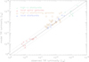 |
Fig. 1. Model TIR luminosity as a function of the TIR luminosity derived from observations. The solid line corresponds to the one-to-one correlation. The dotted lines are located at distances of ±0.3 dex from the solid line. |
The model SFR–IR correlations are presented in Fig. 2. The IR luminosities are measured at 70 μm and between 8 μm and 1000 μm (TIR). We note that there are two high-z starburst galaxies that have significantly lower IR luminosities than the majority of the high-z starburst galaxies. The slopes of both log-log correlations are close to unity, that is, the correlation is close to linear. The slope of the log(SFR)–log(70 μm) correlation is 1.08 ± 0.05, and that of the log(SFR)–log(TIR) correlation is 0.97 ± 0.04.
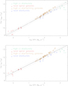 |
Fig. 2. Upper panel: model SFR–70 μm correlation. Lower panel: model SFR–TIR correlation. The solid and dotted lines represent an outlier-resistant linear regression and its uncertainty. The dashed line corresponds to a linear correlation. |
At a given SFR, the low-z starburst galaxies are more similar to the high-z star-forming galaxies in terms of 70 μm luminosities than in terms of TIR luminosities. One might expect the opposite trend because of the higher dust temperatures of the low-z starburst galaxies (⟨Tdust⟩ = 44 K; Vollmer et al. 2017) compared to the high-z star-forming galaxies (⟨Tdust⟩ = 31 K; Vollmer et al. 2017). However, inspection of the two associated modified Planck curves normalized by the TIR luminosity corroborated our result.
The monochromatic and TIR luminosities of the high-z star-forming galaxies are about 50% higher than those of the low-z starbursts at the same SFR. The model TIR luminosity to SFR conversion factors are (0.9 ± 0.4, 1.5 ± 0.4, 0.7 ± 0.2, and 2.4 ± 1.7) × 10−10 M⊙ yr−1  for the local spiral, local starburst, high-z star-forming, and high-z starburst galaxies, respectively. The starburst galaxies therefore show significantly higher TIR luminosity to SFR conversion factors than the main sequence star-forming galaxies. This trend is consistent with the conversion factors based on the observed TIR luminosities for the local galaxies. On the other hand, the model conversion factor of the high-z star-forming galaxies is lower and that of the high-z starburst galaxies is higher than the corresponding conversion factors based on the observationally derived TIR luminosities.
We note that the SFRs of the high-z star-forming galaxies given by Tacconi et al. (2013) lead to model IR spectral density distributions for 14 out of 22 galaxies with well-sampled VizieR SEDs, which are consistent with observations (Fig. C.2). Out of the 16 galaxies with LTIR, model/LTIR, Barro > 1.4, 13 galaxies have a well-sampled VizieR IR SED. Nine of these 13 galaxies have model IR SEDs that are consistent with the VizieR IR SEDs. Within the high-z starburst sample, the model IR SEDs of SMMJ123549+6215 and SMMJ123707+6214 are consistent with the VizieR IR SEDs, whereas they are significantly lower than the VizieR SEDs for SMMJ163650+4057 and SMMJ163658+4105 (Fig. C.6).
We conclude that our model TIR-luminosity-to-SFR conversion factors for the local galaxies are consistent with observations. As expected, the conversion factor of the local spiral galaxies is lower than that of the local starburst galaxies because of additional dust heating in the spiral galaxies by older stellar populations (Rowlands et al. 2014). We might expect the same trend for the high-z galaxies, as predicted by our model. However, the available observationally derived TIR luminosities lead to a common Ṁ∗/LTIR ∼ 1.3 × 10⁻¹⁰ M⊙ yr−1  for the high-z main sequence and starburst galaxies.
5. Results
The velocities of ionized winds are typically hundreds of km s−1 at large radii (several kpc; Veilleux et al. 2005; Heckman et al. 2015). The CR electron advection timescale is tadv = L/vwind, where L is the height of the radio continuum emission and vwind is the mean velocity between z = 0 and z = L. As galactic winds are accelerating with increasing height, the mean wind velocity up to z = L is uncertain. For simplicity, we set L = H. We calculated different wind models (Table 1): with a slow ( ), medium velocity (
 ), and fast wind (
 ). In addition, we calculated models with and without secondary CR electrons, set q = 2.0 and 2.3 (Eq. (8)), and replaced equipartition between the turbulent kinetic and magnetic energy density by (i) B = 5.3 × (Σ/10 M⊙ yr−1) μG (Parker limit; Lacki et al. 2010) where Σ is the gas surface density and (ii)
  μG. The normalizations of the magnetic field strength were chosen such that the model integrated radio continuum emission of the local spiral galaxies are close to observations.
Models.
Before the presentation of the integrated radio continuum spectra calculated by our model, we present the radial profiles of the magnetic field strength, CR electron density and optical depth, and the synchrotron and energy loss timescales of the fiducial model.
5.1. Magnetic field strength and CR density
The median radial profiles of the magnetic field strength, CR electron density, and free-free optical depths of the four galaxy samples are presented in Fig. 3. Whereas the median magnetic field strengths of the low-z starburst and high-z star-forming galaxies are similar within the inner 3 kpc, they are three to four times higher and lower in the high-z starburst galaxies and local spiral galaxies, respectively. The magnetic field strengths in the central kpc are about ∼30 μG, ∼0.5 mG, and ∼2 mG in the local spirals, low-z starbursts/high-z galaxies, and high-z starburst galaxies. This is due to the fact that the turbulent velocity dispersion increases with the SFR (Eq. (A.10)) and the magnetic field strength is proportional to the turbulent velocity dispersion (Eq. (15)).
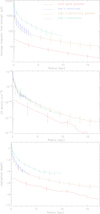 |
Fig. 3. Model median radial profiles of the magnetic field strength (upper panel), CR electron density (middle panel), and free-free optical depth at ν = 1.4 GHz (lower panel) for the four galaxy samples with the associated semi-interquartile ranges. The jumps at R > 10 kpc are caused by taking the median of models with the different radial sizes. |
The median radial profiles of the CR electron density at R > 2 kpc have approximately exponential shapes. The ratios between the profiles of the different samples are significantly smaller than those of the profiles of the magnetic field strength. The CR electron densities of the low-z starbursts, high-z starburst galaxies, and high-z star-forming galaxies are similar, and that of the local spiral galaxies is about a factor of three smaller at a given radius. The exponential scale lengths of the magnetic field strength and the CR electron density are presented in Table 2.
Scale lengths of the magnetic field and the CR electron density in kpc.
The median radial profiles of the free-free optical depths at ν = 1.4 GHz of all galaxy samples are significantly smaller than unity except for the central ∼100 pc of the low-z starbursts and high-z starburst galaxies. Therefore, free-free absorption is expected to play a role in the centers of low-z starbursts and high-z starburst galaxies. Synchrotron self-absorption is negligible for all galaxies in all samples.
5.2. Energy-loss timescales
The radial profiles of the different median model energy-loss timescales (Sect. 2) at 150 MHz, 1.4 GHz, and 5 GHz for the four galaxy samples are presented in Figs. 4 and 5. In the local spiral galaxies the synchrotron, IC, and ionic timescales for ν = 150 MHz are similar for 3 kpc ≲ R ≲ 9 kpc, whereas the bremsstrahlung timescale is about a factor of three lower. At ν = 1.4 GHz, the synchrotron, IC, and bremsstrahlung timescales are similar for 3 kpc ≲ R ≲ 9 kpc, whereas the ionic timescale is about a factor of ten higher. Within the inner 3 kpc, bremsstrahlung leads to the smallest energy loss timescales. At ν = 5 GHz, bremsstrahlung becomes less important because of the decreasing synchrotron and IC timescales with increasing frequency. The advection of CR electrons by galactic winds does not play a role in local spiral galaxies.
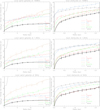 |
Fig. 4. Radial profiles of the different median model timescales for the local spirals (left panels) and low-z starbursts (right panels) at ν = 1.4 GHz (upper panels) and ν = 5 GHz (lower panels) with the associated semi-interquartile ranges. |
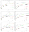 |
Fig. 5. Radial profiles of the different median model timescales for the high-z star-forming galaxies (left panels) and high-z starburst galaxies (right panels) at ν = 1.4 GHz (upper panels) and ν = 5 GHz (lower panels) with the associated semi-interquartile ranges. |
The situation is different in the low-z starbursts. Due to the high magnetic field strengths, the synchrotron timescale is by far the smallest timescale at ν = 5 GHz. At ν = 1.4 GHz, the ionic and bremsstrahlung timescales are comparable to the synchrotron timescale in the inner few hundred parsecs. A fast ( ) wind leads to timescales comparable to the synchrotron timescale. Thus, fast winds are expected to significantly decrease the radio continuum emission of low-z starbursts at ν ≲ 1.4 GHz. At ν = 150 MHz, the ionic timescale is a factor of about three lower than the synchrotron timescale at all radii. The ionic timescale thus sets the CR electron energy loss timescale at this frequency.
In the high-z star-forming galaxies, synchrotron losses dominate within the effective radius (about half of the radial ranges shown in Figs. 4 and 5) at ν = 5 GHz and ν = 1.4 GHz, whereas ionic and bremsstrahlung losses dominate at ν = 150 MHz. Bremsstrahlung losses contribute in the centers, whereas IC losses become more and more important at larger radii. The latter losses dominate beyond the effective radius at all frequencies. Medium velocity winds play an important role for the energy loss of CR electrons within the central 5 kpc.
In the high-z starburst galaxies, the magnetic field strength is so high that the synchrotron losses dominate at all radii at ν = 5 GHz and ν = 1.4 GHz. At ν = 150 MHz, ionic losses dominate for radii smaller than 4 kpc. Energy losses due to galactic winds do not play any role in these galaxies.
5.3. Infrared and radio continuum SEDs
The IR and radio continuum SEDs of the four galaxy samples are presented in Figs. 6 and C.1–C.6. The observed IR and radio continuum flux densities were extracted from the CDS/VizieR database (Ochsenbein et al. 2000). The comparison with Figs. C.1–C.4 of Vollmer et al. (2017) show the significant increase of IR flux density measurements in the VizieR data over the last five years. As stated in Vollmer et al. (2017), the IR SEDs of the galaxies in all samples are reproduced by the model in a satisfactory way.
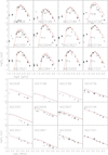 |
Fig. 6. Local spiral galaxies. Crosses mark the observations, and lines show the models. Upper panels: IR SEDs. Data points with significantly lower flux densities are due to measurements within smaller apertures. Lower panels: radio continuum SEDs. Solid red line: Fiducial model. Dashed red line: Wind model. Dashed blue line: sec+wind model. Dotted blue line: sec+fastwind model. |
The different model radio continuum SEDs of the local spiral galaxies (Fig. 6) are very close to each other because neither winds nor secondary CR electrons have a significant effect on the CR electron distributions. The models reproduce the observed radio continuum SEDs within about 50%, except for NGC 628 and NGC 3184 where the model overpredicts the flux densities by a factor of two, and for NGC NGC 3351 where the model overpredicts the flux densities at ν > 1 GHz by a factor of three. Given that the model IR SED also overestimates the VizieR IR SED, the assumed SFR (Leroy et al. 2008) might be overestimated by about a factor of two.
Within the low-z starburst sample, the influence of a wind on the radio continuum SED in models without secondary CR electrons is only significant in three out of nine galaxies. The models with secondaries and a medium velocity wind always lead to significantly higher radio continuum flux densities than observed. Overall, the model that is closest to observations is the fiducial model with a medium-velocity wind (wind; Table 1). The model radio continuum SEDs of IRAS 17208–0014 and IRAS 23365+3604 overpredict the observed SEDs by factors of two to three.
Only 8 out of 44 high-z star-forming galaxies have radio continuum flux density measurements mainly at ν = 1.4 GHz in VizieR. Of these, five model flux densities are close to the observed values whereas two model flux densities are significantly higher and one flux density is significantly lower than observed.
Six out of ten high-z starburst galaxies have radio continuum flux density measurements in VizieR. Four model radio SEDs are close to observations. The remaining two model SEDs overpredict the observed radio continuum flux densities by a factor of ∼3.
We conclude that the observed radio continuum SEDs of most of the local galaxies (spirals and low-z starbursts) and high-z galaxies (main sequence and starbursts) are reproduced by the fiducial model in a satisfactory way. On the other hand, the model significantly overpredicts the observed radio continuum SEDs of ∼25% of the low-z galaxies and ∼35% of the high-z galaxies.
5.4. Alternative magnetic field strength and CR energy distribution prescriptions
The influence of the different recipes for the magnetic field strength can best be recognized in the radio continuum SEDs of the low-z starburst sample (Fig. 7). The radio continuum SEDs of the models involving (i) equipartition between the turbulent kinetic and magnetic energy densities and (ii) B = 5.3 × (Σ/10 M⊙ yr−1) μG are similar. Compared to equipartition, the latter recipe leads to ∼10% higher radio continuum flux densities. On the other hand, the recipe  G leads to radio continuum flux densities, which are significantly smaller than observed (up to a factor of ten) for five out of nine low-z starbursts. Models of IRAS 17208–004, Arp 220D, and IRAS 23365+3604 with faster winds naturally lead to better reproductions of the observed radio continuum SEDs. We therefore believe that the recipe involving only the gas density does not reproduce the available observations and should be discarded.
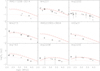 |
Fig. 7. Radio continuum SEDs of the low-z starbursts. Solid line: Fiducial model. Dashed line: B = 5.3 × (Σ/10 M⊙ yr−1) μG. Dotted line: |
The use of an exponent for the energy dependence of the primary CR injection of q = 2.3 instead of q = 2.0 leads to ∼50% higher CR electron densities than those of the fiducial model and to exponents of the IR–radio correlations that are higher by ∼0.1 compared to the exponents of the fiducial model. Furthermore, the radio continuum SEDs become steeper and the radio continuum luminosities of the low-z starbursts, high-z star-forming, and high-z starburst galaxies become ∼50% higher compared to the values of the fiducial model. Therefore, the q = 2.3 models are less good at reproducing the radio continuum emission of the low-z starburst and high-z galaxy samples.
5.5. The IR–radio correlation
As our fiducial model is our preferred model, we only show and discuss the SFR–IR, IR–radio, and SFR–radio correlations for this model.
The monochromatic (70, 100, 160 μm) and TIR–radio correlations of all four samples are shown in Fig. 8. We calculated the slopes and offsets of the correlation using an outlier-resistant bisector fit. The results can be found together with the correlation scatter in Fig. 8.
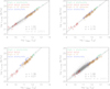 |
Fig. 8. Upper left: 70 μm–1.4 GHz correlation. Upper right: 100 μm–1.4 GHz correlation. Lower left: 160 μm–1.4 GHz correlation. Lower right: TIR–1.4 GHz correlation. Colored symbols show model galaxies. Black solid and dotted lines mark the model linear regression. Gray dots show observations. |
The exponents derived from the bisector fits of the monochromatic IR–radio correlations increase with increasing wavelength from 1.00 at 70 μm to 1.15 at 100 μm, and 1.38 at 160 μm. The exponent of the TIR–radio correlation is 1.08. These slopes are consistent with those derived with a Bayesian approach, the uncertainties of which are about 0.05 (Table 3). The corresponding exponents found by Molnár et al. (2021) are 1.01 ± 0.01, 1.05 ± 0.09, and 1.17 ± 0.13 at 60, 100, and 160 μm. That of the TIR–radio correlation is 1.11 ± 0.01. There is therefore agreement within 0.2, 1.0, 1.5, and 0.6σ of the joint uncertainty of model and data. The associated scatters of the data around the power-law correlation are ∼0.2 dex for all four correlations.
Correlation fits with Bayesian approach.
Furthermore, we used the Bayesian approach to linear regression with errors in both directions (Kelly 2007). We assumed uncertainties on the TIR and radio luminosities of 0.2 dex for the local galaxies and 0.3 dex for the high-z galaxies. For a direct comparison we also calculated the slopes and offsets for the data of Yun et al. (2001; uncertainties of 0.05 dex in both directions) and Molnár et al. (2021; symmetrized mean TIR luminosity uncertainties). As small deviations of the correlation slope lead to large deviations of the offset at log(LIR) = 0, we decided to calculate the offsets at an IR luminosity of 1010 L⊙. The resulting slopes and offsets derived by the Bayesian approach are presented in Table 3. There is agreement between the slopes within 0.5σ and between the offsets within 2σ of the joint uncertainty of model and data for both datasets.
Bell (2003) assembled a diverse sample of local galaxies from the literature with FUV, optical, IR, and radio luminosities and found a nearly linear radio–IR correlation. The left panel of Fig. 9 shows the direct comparison between our local model galaxies (spirals and low-z starbursts) and the compilation of Bell (2003). As before, we assumed uncertainties of 0.2 dex for the model TIR and radio luminosities. There is agreement between the slopes within 0.1σ and between the offsets within 0.4σ of the joint uncertainty of model and data (Table 3).
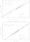 |
Fig. 9. TIR–1.4 GHz correlations. Colored symbols show model galaxies. Black solid and dotted lines show the model linear regression. Upper panel: gray solid and dotted lines show the observed linear regression (Basu et al. 2015). Lower panel: gray error bars show data from Bell (2003). Gray solid and dashed lines mark the observed linear regression (Bell 2003). |
Basu et al. (2015) studied the radio–TIR correlation in star-forming galaxies chosen from the PRism MUltiobject Survey up to redshift of 1.2 in the XMM-LSS field, employing the technique of image stacking. These authors found a exponent of the TIR–1.4 GHz correlation of 1.11 ± 0.04. The upper left panels of Fig. 9 show the direct comparison between our model galaxies (local and high-redshift) and those of Basu et al. (2015) show comparable exponents and scatters. There is agreement between the slopes within 0.4σ of the joint uncertainty of model and data (Table 3).
The radio–FIR correlation is generally quantified via the parameter qIR defined as qIR = log(LIR/Lradio). Following Helou et al. (1985), we define for the bolometric case
 (25)
(25)
We compared the TIR luminosity integrated between 8 and 1000 μm, the FIR luminosity, which is typically integrated between 40 and 120 μm (for a consistent comparison with our model, we integrated the model IR SEDs between 70 μm and 160 μm), and the monochromatic luminosity at 70 μm.
We compiled IR-to-radio luminosity ratios for different galaxy types from the literature (Table 4) and compared them to the values of our model qIR (Table 5). We divided our samples into local galaxies (spirals and low-z starbursts) and total sample (spirals, low-z starbursts, high-z star-forming, and high-z starburst galaxies). The literature samples are relatively well matched to the model samples in terms of IR luminosity and redshift ranges (Table 4). In the cases where two groups determined qIR independently for a given galaxy sample, the values are consistent, except for the TIR–radio correlation of high-z starburst galaxies, where the difference exceeds 0.3 dex between the value of Thomson et al. (2019) and that of Algera et al. (2020).
Galaxy samples for the calculation of IR-to-radio luminosity ratios.
IR-to-radio ratio.
As expected, the IR-to-radio luminosity ratios of the different models are comparable for the local spirals. Moreover, the inclusion of a wind increases qIR whereas the inclusion of secondaries decreases qIR. The magnetic field strength recipe involving the gas surface density (model Bsigma) does not significantly change qIR, whereas the recipe involving the gas density (model Brho) leads to the highest qIR values for all galaxy samples except the local spirals and high-z starburst galaxies. As these values are significantly higher than the observed ones, we can discard model Brho.
The TIR-to-radio luminosity ratios of our fiducial model are consistent (within 0.2 dex or 2σ) with observations for the local high-z star-forming galaxies and the total sample. The TIR-to-radio luminosity ratios of the high-z starburst galaxies is consistent within 0.5σ with those of Algera et al. (2020) and Thomson et al. (2019). However, it is 6σ higher than the value found by Thomson et al. (2014). The model TIR-to-radio luminosity ratios of the low-z starbursts deviate from the observed value by 0.3 dex or 3σ. Based on the observed high qTIR of the low-z starbursts, a median velocity or fast galactic wind is needed in the absence or presence of secondary CR electrons, respectively.
The FIR-to-radio luminosity ratios of our fiducial model are consistent with observations (within 0.7σ) for the local galaxies and the high-z star-forming galaxies. The model FIR-to-radio luminosity ratios of the high-z starburst galaxies deviate from the observed value by 0.3 dex (or 2σ). The 70 μm-to-radio luminosity ratios of our fiducial model are consistent with observations (within 1σ) for the low-z starbursts, local galaxies, and the total sample. The production of secondary CR electrons, which decreases qIR, is not needed in the framework of our model. We conclude that our fiducial model of the main sequence star-forming galaxies is consistent with the available IR-to-radio luminosity ratios determined by observations. The low-z starburst models probably need a galactic wind.
5.6. The SFR–radio correlation
The model SFR–1.4 GHz and SFR–150 MHz correlations are presented in Fig. 10 together with the observed correlations. The SFRs were derived using different methods and the correlations were derived for different samples (Table 6). The exponents of the SFR–radio correlations based on SED-fitting methods are smaller than the exponents based on IR luminosities and extinction-corrected Hα. For SFRs derived through extinction-corrected Hα and IR luminosities, the exponents tend to unity if low-z starbursts with Ṁ∗ > 10 M⊙ yr−1 are included in the sample. It appears that the exponent of the SFR–150 MHz correlation is somewhat steeper than that of the SFR–1.4 GHz correlation.
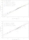 |
Fig. 10. Upper panel: SFR–1.4 GHz correlation. Lower panel: SFR–150 MHz correlation. Colored lines show observed correlations. Plus symbols mark model galaxies. |
Exponents of the SFR–radio correlation.
We found an exponent of the model SFR–1.4 GHz correlation for the combined sample of 1.05 ± 0.04. The normalization is log(L1.4 GHz/(W Hz−1)) = 21.43 ± 0.08 with an additional systematic uncertainty of ±0.15 stemming from the comparison between the model and observed IR–radio offsets measured by Yun et al. (2001) and Molnár et al. (2021). The slope is close to that of Heesen et al. (2014), somewhat steeper than those of Bell (2003) and Murphy et al. (2011), and shallower than that of Boselli et al. (2015). However, the model radio luminosities are a factor of two higher than the radio luminosities observed by Boselli et al. (2015). Alternatively, dividing the SFRs of these authors by a factor of two would make the model and observed correlations identical. The model slope is close to (1σ) that found by Heesen et al. (2014), lower (4σ) than that of Brown et al. (2017), and significantly higher (19σ) than that of Gürkan et al. (2018).
The exponent of the model SFR–150 MHz correlation for the combined sample is 0.99 ± 0.05. This is consistent with the exponents found by Gürkan et al. (2018; 1.6σ) and Smith et al. (2021; 1σ). The slope found by Wang et al. (2019) is higher by 5σ than our model slope. The normalization of the model correlation is log(L150 MHz/(W Hz−1)) = 21.93 ± 0.1.
We conclude that the observed SFR–radio correlation can be reproduced by our fiducial model in a reasonable way (within ∼4σ). The model exponents are very close to one.
6. Discussion
The agreement between the slopes of the model and observed IR–radio correlation (2σ) is better than that between the slopes of the model and observed SFR–radio correlation (4σ). We note that, whereas the SFR is an input quantity, the IR emission is calculated by the model. The poorer agreement for the SFR–radio correlation is at least partly due to the relatively large scatter of the different measurements (1.10 ± 0.16 at 1.4 GHz and 1.15 ± 0.17 at 150 MHz; Table 6). This observational scatter should be decreased by about a factor of two before we can think about improvements of the model. Possible improvements are a better inclusion of radio halos (Eq. (21); Krause et al. 2018), a more sophisticated description of the vertical CR electron diffusion (Eq. (10)), the explicit inclusion of CR protons, and a better description of the IR emission of the warm ISM.
Gürkan et al. (2018), Smith et al. (2021), and Delvecchio et al. (2021) found a mass-dependent IR–radio correlation. Galaxies of higher masses have lower IR-to-radio luminosity ratios. Unfortunately, the mass range of our model galaxy samples is not broad enough to show a mass dependence of qIR.
In Sect. 5.3 it was shown that our fiducial model overpredicts the radio continuum emission of 25% of the low-z starbursts. Our low-z starburst sample (log(⟨LTIR/L⊙⟩) = 12) has a lower model TIR-to-radio luminosity ratio than the local spiral sample (Sect. 5.5). This is contrary to the observed TIR-to-radio luminosity ratios, which are higher for the low-z starbursts than for the local spiral galaxies. For the high-z starburst galaxies, the situation is less clear. Whereas our fiducial model overpredicts the radio continuum emission of 35% of the high-z starburst galaxies, the model IR-to-radio luminosity ratios are significantly higher than those found by Thomson et al. (2014) but are comparable to those found by Thomson et al. (2019) and Algera et al. (2020) (Table 5). The latter authors ascribe the difference with respect to Thomson et al. (2014) to the fact that they used a stacking technique, which allowed them to reach lower IR and radio luminosities. We might observe such a trend in our low-z starburst model compared to observations. However, the high-z starburst galaxies of Table B.3 have rather low IR-to-radio luminosity ratios (qTIR = 2.2) despite their high TIR luminosities (log(⟨LTIR/L⊙⟩) = 13). Significantly higher TIR-to-radio luminosity ratios can be achieved via fast galactic winds in the absence of secondary CR electrons.
Models including secondary CR electrons are also viable for low-z starbursts and high-z galaxies but only in the presence of fast galactic winds (Table 5). The simple prescription of the advection timescale based on the rotation velocity (Eq. (11)) is not sufficient to yield model radio luminosities that are comparable to observations. We note that the wind velocities measured by Rupke et al. (2002) of ∼500 km s−1 correspond to a medium- velocity wind ( ). However, the low-z starburst models with secondary CR electrons need a fast wind of ten times this latter velocity to reproduce observations (Table 5).
As stated in Sect. 1, noncalorimeter models often have to involve a conspiracy to maintain the tightness of the FIR–radio correlation. The fiducial models closest to CR electron calorimeters are the models of the starburst galaxies (low-z starburst and high-z starburst galaxies; right panels of Fig. 5). The situation changes if fast winds are added to the models. Lacki et al. (2010) stated that IC cooling alone is very quick in starbursts, implying that electrons cannot escape from these galaxies before losing most of their energy (Condon et al. 1991; Thompson et al. 2006). This is not the case in our starburst samples (low-z starbursts and high-z starburst galaxies, upper panels of Figs. 4 and 5). The synchrotron timescale is much smaller than the IC timescale. This is due to equipartition between the turbulent kinetic and magnetic field energy densities. It is not only the density that is enhanced in the starburst galaxies but also the turbulent velocity dispersion (Downes & Solomon 1998; Genzel et al. 2010; Tacconi et al. 2013; Vollmer et al. 2017). This is why our model starburst galaxies can be considered as close to CR electron calorimeters. On the other hand, the model spiral galaxies and high-z star-forming galaxies are not CR electron calorimeters. In both galaxies, energy losses due to bremsstrahlung and IC cooling are important.
To quantify the effect of the different CR electron energy losses, we made model calorimeter calculations by setting tdiff = twind = tIC = tbrems = tion = 0. The resulting IR–radio correlations are shown in Fig. 11 and can be directly compared to the upper left and lower right panels of Fig. 8. As expected, the radio continuum luminosities of all galaxies increase: those of the high-z starburst galaxies by ∼0.3 dex, and those of the local spiral galaxies by ∼0.8 dex. Most importantly, the slope of the correlation flattens (0.9 instead of 1.1 at 70 μm and 1.0 instead of 1.2 for the TIR). We note that the exponent is not unity in our fiducial model because the SFR–FIR correlation is slightly superlinear. This slope is significantly different from the observed slope (see Table 6). Furthermore, the model radio continuum SEDs of the calorimeter model have much steeper slopes than observed for the local spiral galaxies, low-z starbursts, and high-z starburst galaxies.
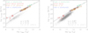 |
Fig. 11. Calorimeter models. TIR–1.4 GHz correlation. Colored symbols mark the model galaxies, black solid and dotted lines show the model linear regression, and gray dots show observations. |
For a further investigation of the influence of the different CR electron energy loss times on the TIR–1.4 GHz correlation, we set all timescales but one to zero. The slopes and normalizations of the resulting TIR–radio correlation are presented in Table D.1 and Fig. D.1. Advective and ionic energy losses do not play a role in our models. The slope and normalization of our fiducial model are set by diffusion, bremsstrahlung, and IC losses.
Averaged over sufficiently long length- and timescales, the CR distribution may achieve energy equipartition with the magnetic field (Beck & Krause 2005). It is not known whether or not most synchrotron sources are in equipartition between the CR particle and magnetic field energy densities, but radio astronomers often assume so because it is physically plausible (CRs and magnetic fields have a common source of energy, which are supernova explosions, and CRs are confined by magnetic fields) and this allows estimation of the relativistic particle energies and the magnetic field strengths of radio sources with measured luminosities and sizes. However, as stated by Seta et al. (2018), there is no compelling observational or theoretical reason to expect a tight correlation between the CR particle and the magnetic field energy densities across all scales. For a recent review on CR–magnetic field equipartition; see Seta & Beck (2019). Most of the energy of CRs is carried by protons and heavier particles, and therefore the equipartition assumption relies on the assumption that relativistic electrons are distributed similarly to the heavier CR particles. Energy equipartition can therefore be written as
 (26)
(26)
where η is the fraction of energy in heavy CR particles, me the electron mass, and c the speed of light. For strong shocks in nonrelativistic gas, η ∼ 40 (Beck & Krause 2005). This corresponds to a proton-to-electron number ratio of 40 which is only a factor of two lower than the observed value (e.g., Yoshida 2008). We caution the reader that the calculation of the CR electron energy density strongly depends on the assumed lower energy cutoff γ2 and on the exponent of nCRe(γ).
The ratios between the magnetic and CR electron energy densities are presented for the different galaxy samples in Fig. 12. The ratios UB/Ue of most of the local spiral galaxies are between 10 and 20, consistent with resonant scattering of Alfvén waves within the turbulent ISM (Beck & Krause 2005). The majority of the high-z star-forming galaxies have UB/Ue ∼ 200, which is higher than the value predicted for strong shocks (UB/Ue ∼ 40; Beck & Krause 2005). The starburst galaxies have much higher ratios (UB/Ue > 100). This is expected because the variation of the magnetic field strengths between the different samples is much larger than that of the CR electron densities (Fig. 3). Our result is consistent with the findings of Yoast-Hull et al. (2016) who found a significantly larger magnetic field energy density than the CR energy density in starburst galaxies. We therefore conclude that energy equipartition between the CR particles and the magnetic field approximately holds in our models of star-forming galaxies.
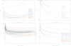 |
Fig. 12. Ratios between the magnetic and CR electron energy densities. Upper left: local spiral galaxies. Upper right: low-z starbursts. Lower left: high-z star-forming galaxies. The kink in the radial profiles is caused by the sudden onset of a galactic wind. Lower right: high-z starburst galaxies. |
7. Conclusions
In galaxies, not all the injected energy of CR electrons is radiated via synchrotron emission, meaning that galaxies cannot be treated as electron calorimeters. Multiple energy losses of CR electrons decrease the synchrotron emission: IC losses, bremsstrahlung, diffusion of CR electrons into the galactic halo, advection of CR electrons by galactic wind, and ionic losses. The mixture of these losses shapes the radio continuum SED. We extended the analytical model of galactic disks of Vollmer et al. (2017) by including a simplified prescription for the synchrotron emissivity (Eq. (19)). The galactic gas disks are treated as turbulent clumpy accretion disks. The different losses are taken into account via their characteristic timescales. The magnetic field strength is determined by the equipartition between the turbulent kinetic and the magnetic energy densities. In this way, the radio luminosities of the Vollmer et al. (2017) model galaxies were calculated: local spiral galaxies, low-z starburst galaxies, high-z main sequence star-forming galaxies, and high-z starburst galaxies. Based on the comparison between our model galaxies and available observations, we come to the following conclusions:
-
The exponents of the model log(SFR)–log(70 μm) and log(SFR)–log(TIR) correlations are close to one (1.09 ± 0.02 and 0.98 ± 0.03; Sect. 4).
-
The ratio between the magnetic field strength of the different samples is much higher than the ratio between the CR electron densities. Free-free absorption mainly affects the centers of the starburst galaxies (low-z starbursts and high-z starbursts) at frequencies lower than 1 GHz (Sect. 5.1).
-
In local spiral galaxies and high-z star-forming galaxies, IC energy losses and losses due to bremsstrahlung are significant in the outer and inner disks, respectively. At low frequencies (ν ∼ 150 MHz) ionic losses become important in the inner disks. The models of the starburst galaxies are close to calorimetric if no fast galactic winds are included (Sect. 5.2).
-
The observed radio continuum SEDs of most (∼70%) of the galaxies are reproduced by the fiducial model in a satisfactory way. Except for the local spiral galaxies, fast galactic winds can potentially make conflicting models agree with observations (Sect. 5.3).
-
The comparison with data of Yun et al. (2001), Bell (2003), Basu et al. (2015), and Molnár et al. (2021) shows agreement within 2σ between the model and observed IR–radio correlations. Our fiducial model is also consistent with the available IR-to-radio luminosity ratios determined by observations. Only the low-z starburst models probably need a galactic wind (Sect. 5.5).
-
The observed SFR–radio correlations at 150 MHz and 1.4 GHz can be reproduced by our fiducial model within ∼4σ of the joint uncertainty of model and data for both datasets. The model exponents are 0.99 ± 0.05 and 1.05 ± 0.04 at 150 MHz and 1.4 GHz, respectively (Sect. 5.6).
-
Advective and ionic energy losses do not play a significant role in our model TIR–1.4 GHz correlations. The slope and normalization of our fiducial model are set by diffusion, bremsstrahlung, and inverse Compton losses. If a CR electron calorimeter is assumed, the slope of the IR–1.4 GHz correlation flattens: 0.9 instead of 1.1 at 70 μm and 1.0 instead of 1.2 for the TIR (Fig. 11).
-
Equipartition between the turbulent kinetic and magnetic field energy densities seems to be realized in the gas disks of star-forming and starburst galaxies.
-
Energy equipartition between the CR particles and the magnetic field only approximately holds in our models of main sequence star-forming galaxies (Fig. 12).
-
Inverse Compton losses are not dominant in the starburst galaxies because in these galaxies, not only the gas density but also the turbulent velocity dispersion is higher than in normal star-forming galaxies. Equipartition between the turbulent kinetic and magnetic field energy densities then leads to very high magnetic field strengths and very short synchrotron timescales.
Our fiducial model reproduces the available IR and radio data in a satisfactory way. However, the role of CR electron secondaries and galactic winds must still be elucidated in the framework of our model. In particular, our simple prescription of the wind timescale (Eq. (11)) is not able to reproduce the available data in the presence of CR electron secondaries. The inclusion of a sample of luminous IR galaxies bridging parameter space between local spirals and low-z starburst galaxies will certainly be helpful.
Acknowledgments
We would like to thank R. Beck and the anonymous referee for their comments, which helped to significantly improve the article.
References
- Aharonian, F. A., Kelner, S. R., & Prosekin, A. Y. 2010, Phys. Rev. D, 82, 043002 [Google Scholar]
- Algera, H. S. B., Smail, I., Dudzevičiūtė, U., et al. 2020, ApJ, 903, 138 [Google Scholar]
- Appleton, P. N., Fadda, D. T., Marleau, F. R., et al. 2004, ApJS, 154, 147 [Google Scholar]
- Barro, G., Pérez-González, P. G., Gallego, J., et al. 2011, ApJS, 193, 30 [Google Scholar]
- Basu, A., Wadadekar, Y., Beelen, A., et al. 2015, ApJ, 803, 51 [NASA ADS] [CrossRef] [Google Scholar]
- Beck, R., & Krause, M. 2005, Astron. Nachr., 326, 414 [Google Scholar]
- Beck, R. 2015, A&ARv, 24, 4 [Google Scholar]
- Bell, E. F. 2003, ApJ, 586, 794 [Google Scholar]
- Boselli, A., Fossati, M., Gavazzi, G., et al. 2015, A&A, 579, A102 [NASA ADS] [CrossRef] [EDP Sciences] [Google Scholar]
- Bothwell, M. S., Smail, I., Chapman, S. C., et al. 2013, MNRAS, 429, 3047 [Google Scholar]
- Brown, M. J. I., Moustakas, J., Kennicutt, R. C., et al. 2017, ApJ, 847, 136 [Google Scholar]
- Chabrier, G. 2003, ApJ, 586, L133 [NASA ADS] [CrossRef] [Google Scholar]
- Chapman, S. C., Ivison, R. J., Roseboom, I. G., et al. 2010, MNRAS, 409, L13 [NASA ADS] [CrossRef] [Google Scholar]
- Condon, J. J., Huang, Z.-P., Yin, Q. F., et al. 1991, ApJ, 378, 65 [NASA ADS] [CrossRef] [Google Scholar]
- Condon, J. J. 1992, ARA&A, 30, 575 [Google Scholar]
- Connell, J. J. 1998, ApJ, 501, L59 [NASA ADS] [CrossRef] [Google Scholar]
- Dale, D. A., Aniano, G., Engelbracht, C. W., et al. 2012, ApJ, 745, 95 [NASA ADS] [CrossRef] [Google Scholar]
- Davies, L. J. M., Huynh, M. T., Hopkins, A. M., et al. 2017, MNRAS, 466, 2312 [Google Scholar]
- Delhaize, J., Smolčić, V., Delvecchio, I., et al. 2017, A&A, 602, A4 [NASA ADS] [CrossRef] [EDP Sciences] [Google Scholar]
- Delvecchio, I., Daddi, E., Sargent, M. T., et al. 2021, A&A, 647, A123 [NASA ADS] [CrossRef] [EDP Sciences] [Google Scholar]
- Downes, D., & Solomon, P. M. 1998, ApJ, 507, 615 [NASA ADS] [CrossRef] [Google Scholar]
- Elmegreen, B. G. 1989, ApJ, 338, 178 [NASA ADS] [CrossRef] [Google Scholar]
- Farrah, D., Afonso, J., Efstathiou, A., et al. 2003, MNRAS, 343, 585 [Google Scholar]
- Genzel, R., Tacconi, L. J., Gracia-Carpio, J., et al. 2010, MNRAS, 407, 2091 [NASA ADS] [CrossRef] [Google Scholar]
- Graciá-Carpio, J., García-Burillo, S., Planesas, P., et al. 2008, A&A, 479, 703 [NASA ADS] [CrossRef] [EDP Sciences] [Google Scholar]
- Gürkan, G., Hardcastle, M. J., Smith, D. J. B., et al. 2018, MNRAS, 475, 3010 [Google Scholar]
- Heckman, T. M., Norman, C. A., Strickland, D. K., et al. 2002, ApJ, 577, 691 [NASA ADS] [CrossRef] [Google Scholar]
- Heckman, T. M., Alexandroff, R. M., Borthakur, S., et al. 2015, ApJ, 809, 147 [NASA ADS] [CrossRef] [Google Scholar]
- Heesen, V., Brinks, E., Leroy, A. K., et al. 2014, AJ, 147, 103 [NASA ADS] [CrossRef] [Google Scholar]
- Heesen, V., Buie, E., Huff, C. J., et al. 2019, A&A, 622, A8 [NASA ADS] [CrossRef] [EDP Sciences] [Google Scholar]
- Helou, G., & Bicay, M. D. 1993, ApJ, 415, 93 [Google Scholar]
- Helou, G., Soifer, B. T., & Rowan-Robinson, M. 1985, ApJ, 298, L7 [Google Scholar]
- Inoue, A. K., Hirashita, H., & Kamaya, H. 2000, PASJ, 52, 539 [NASA ADS] [CrossRef] [Google Scholar]
- Jarvis, M. J., Smith, D. J. B., Bonfield, D. G., et al. 2010, MNRAS, 409, 92 [Google Scholar]
- Kelly, B. C. 2007, ApJ, 665, 1489 [Google Scholar]
- Kennicutt, R. C. 1998, ARA&A, 36, 189 [NASA ADS] [CrossRef] [Google Scholar]
- Kovács, A., Chapman, S. C., Dowell, C. D., et al. 2006, ApJ, 650, 592 [CrossRef] [Google Scholar]
- Krause, M., Irwin, J., Wiegert, T., et al. 2018, A&A, 611, A72 [NASA ADS] [CrossRef] [EDP Sciences] [Google Scholar]
- Kregel, M., van der Kruit, P. C., & de Grijs, R. 2002, MNRAS, 334, 646 [NASA ADS] [CrossRef] [Google Scholar]
- Kroupa, P., Tout, C. A., & Gilmore, G. 1993, MNRAS, 262, 545 [NASA ADS] [CrossRef] [Google Scholar]
- Krumholz, M. R., Dekel, A., & McKee, C. F. 2012, ApJ, 745, 69 [Google Scholar]
- Lacki, B. C., Thompson, T. A., & Quataert, E. 2010, ApJ, 717, 1 [Google Scholar]
- Larson, R. B. 1981, MNRAS, 194, 809 [Google Scholar]
- Leroy, A. K., Walter, F., Brinks, E., et al. 2008, AJ, 136, 2782 [Google Scholar]
- Leroy, A. K., Walter, F., Bigiel, F., et al. 2009, AJ, 137, 4670 [Google Scholar]
- Li, J.-T., Beck, R., Dettmar, R.-J., et al. 2016, MNRAS, 456, 1723 [NASA ADS] [CrossRef] [Google Scholar]
- Licquia, T. C., & Newman, J. A. 2015, ApJ, 806, 96 [NASA ADS] [CrossRef] [Google Scholar]
- Lizée, T., Vollmer, B., Braine, J., et al. 2022, A&A, 663, A152 [NASA ADS] [CrossRef] [EDP Sciences] [Google Scholar]
- Madau, P., & Dickinson, M. 2014, ARA&A, 52, 415 [Google Scholar]
- Magnelli, B., Lutz, D., Santini, P., et al. 2012, A&A, 539, A155 [NASA ADS] [CrossRef] [EDP Sciences] [Google Scholar]
- Magnelli, B., Ivison, R. J., Lutz, D., et al. 2015, A&A, 573, A45 [NASA ADS] [CrossRef] [EDP Sciences] [Google Scholar]
- Mannheim, K., & Schlickeiser, R. 1994, A&A, 286, 983 [NASA ADS] [Google Scholar]
- Mauch, T., & Sadler, E. M. 2007, MNRAS, 375, 931 [Google Scholar]
- Molnár, D. C., Sargent, M. T., Leslie, S., et al. 2021, MNRAS, 504, 118 [CrossRef] [Google Scholar]
- Murphy, E. J. 2009, ApJ, 706, 482 [Google Scholar]
- Murphy, E. J., Chary, R.-R., Dickinson, M., et al. 2011, ApJ, 732, 126 [NASA ADS] [CrossRef] [Google Scholar]
- Murphy, E. J., Bremseth, J., Mason, B. S., et al. 2012, ApJ, 761, 97 [Google Scholar]
- Niklas, S., & Beck, R. 1997, A&A, 320, 54 [NASA ADS] [Google Scholar]
- Ochsenbein, F., Bauer, P., & Marcout, J. 2000, A&AS, 143, 23 [NASA ADS] [CrossRef] [EDP Sciences] [Google Scholar]
- Read, S. C., Smith, D. J. B., Gürkan, G., et al. 2018, MNRAS, 480, 5625 [Google Scholar]
- Rémy-Ruyer, A., Madden, S. C., Galliano, F., et al. 2014, A&A, 563, A31 [Google Scholar]
- Rovilos, E., Diamond, P. J., Lonsdale, C. J., et al. 2002, Proceedings of the 6th EVN Symposium, 179 [Google Scholar]
- Rowlands, K., Dunne, L., Dye, S., et al. 2014, MNRAS, 441, 1017 [NASA ADS] [CrossRef] [Google Scholar]
- Rozwadowska, K., Vissani, F., & Cappellaro, E. 2021, New Astron., 83, 101498 [NASA ADS] [CrossRef] [Google Scholar]
- Rupke, D. S., Veilleux, S., & Sanders, D. B. 2002, ApJ, 570, 588 [NASA ADS] [CrossRef] [Google Scholar]
- Sargent, M. T., Schinnerer, E., Murphy, E., et al. 2010, ApJ, 714, L190 [Google Scholar]
- Schleicher, D. R. G., & Beck, R. 2013, A&A, 556, A142 [NASA ADS] [CrossRef] [EDP Sciences] [Google Scholar]
- Scoville, N., Murchikova, L., Walter, F., et al. 2017, ApJ, 836, 66 [Google Scholar]
- Seta, A., & Beck, R. 2019, Galaxies, 7, 45 [NASA ADS] [CrossRef] [Google Scholar]
- Seta, A., Shukurov, A., Wood, T. S., et al. 2018, MNRAS, 473, 4544 [NASA ADS] [CrossRef] [Google Scholar]
- Smith, D. J. B., Haskell, P., Gürkan, G., et al. 2021, A&A, 648, A6 [EDP Sciences] [Google Scholar]
- Speagle, J. S., Steinhardt, C. L., Capak, P. L., et al. 2014, ApJS, 214, 15 [NASA ADS] [CrossRef] [Google Scholar]
- Tabatabaei, F. S., Berkhuijsen, E. M., Frick, P., et al. 2013, A&A, 557, A129 [NASA ADS] [CrossRef] [EDP Sciences] [Google Scholar]
- Tacconi, L. J., Neri, R., Genzel, R., et al. 2013, ApJ, 768, 74 [NASA ADS] [CrossRef] [Google Scholar]
- Thompson, T. A., Quataert, E., Waxman, E., et al. 2006, ApJ, 645, 186 [NASA ADS] [CrossRef] [Google Scholar]
- Thomson, A. P., Ivison, R. J., Simpson, J. M., et al. 2014, MNRAS, 442, 577 [NASA ADS] [CrossRef] [Google Scholar]
- Thomson, A. P., Smail, I., Swinbank, A. M., et al. 2019, ApJ, 883, 204 [Google Scholar]
- Thornton, K., Gaudlitz, M., Janka, H.-T., et al. 1998, ApJ, 500, 95 [CrossRef] [Google Scholar]
- Tsang, O. 2007, PhD Dissertation, Ruperto-Carola University of Heidelberg, Germany [Google Scholar]
- Valiante, E., Lutz, D., Sturm, E., et al. 2009, ApJ, 701, 1814 [NASA ADS] [CrossRef] [Google Scholar]
- Veilleux, S., Cecil, G., & Bland-Hawthorn, J. 2005, ARA&A, 43, 769 [NASA ADS] [CrossRef] [Google Scholar]
- Voelk, H. J. 1989, A&A, 218, 67 [NASA ADS] [Google Scholar]
- Vollmer, B., & Beckert, T. 2003, A&A, 404, 21 [NASA ADS] [CrossRef] [EDP Sciences] [Google Scholar]
- Vollmer, B., & Leroy, A. K. 2011, AJ, 141, 24 [Google Scholar]
- Vollmer, B., Davoust, E., Dubois, P., et al. 2005, A&A, 431, 1177 [NASA ADS] [CrossRef] [EDP Sciences] [Google Scholar]
- Vollmer, B., Gassmann, B., Derrière, S., et al. 2010, A&A, 511, A53 [NASA ADS] [CrossRef] [EDP Sciences] [Google Scholar]
- Vollmer, B., Gratier, P., Braine, J., et al. 2017, A&A, 602, A51 [NASA ADS] [CrossRef] [EDP Sciences] [Google Scholar]
- Vollmer, B., Soida, M., Beck, R., et al. 2020, A&A, 633, A144 [NASA ADS] [CrossRef] [EDP Sciences] [Google Scholar]
- Vollmer, B., Braine, J., Mazzilli-Ciraulo, B., et al. 2021, A&A, 647, A138 [CrossRef] [EDP Sciences] [Google Scholar]
- Walter, F., Brinks, E., de Blok, W. J. G., et al. 2008, AJ, 136, 2563 [Google Scholar]
- Wang, L., Gao, F., Duncan, K. J., et al. 2019, A&A, 631, A109 [NASA ADS] [CrossRef] [EDP Sciences] [Google Scholar]
- Webber, W. R., McDonald, F. B., & Lukasiak, A. 2003, ApJ, 599, 582 [NASA ADS] [CrossRef] [Google Scholar]
- Werhahn, M., Pfrommer, C., & Girichidis, P. 2021a, MNRAS, 505, 3295 [NASA ADS] [CrossRef] [Google Scholar]
- Werhahn, M., Pfrommer, C., Girichidis, P., et al. 2021b, MNRAS, 505, 3273 [NASA ADS] [CrossRef] [Google Scholar]
- Yoast-Hull, T. M., Gallagher, J. S., & Zweibel, E. G. 2016, MNRAS, 457, L29 [NASA ADS] [CrossRef] [Google Scholar]
- Yoshida, K. 2008, Adv. Space Res., 42, 477 [NASA ADS] [CrossRef] [Google Scholar]
- Yun, M. S., Reddy, N. A., & Condon, J. J. 2001, ApJ, 554, 803 [Google Scholar]
Appendix A: The large-scale model
Following Vollmer & Leroy (2011), the ISM is considered as a single turbulent gas in vertical hydrostatic equilibrium. The turbulent pressure is  , where
  is the total 3D velocity dispersion that takes into account both the turbulent velocity dispersion vturb and a constant thermal velocity vtherm = cs = 6 km s−1. Following Elmegreen (1989), hydrostatic pressure equilibrium is given by
 (A.1)
(A.1)
where Σ is the total gas surface density, Σ⋆ is the stellar surface density, and  is the vertical stellar velocity dispersion. Given the stellar surface density and the stellar length scale of the disk l⋆, the vertical stellar velocity dispersion is given according to Kregel et al. 2002):
 (A.2)
(A.2)
Turbulence in the ISM is mainly maintained by energy input via supernova explosions giving rise to a turbulent driving length scale ldriv. The energy per unit time which is dissipated by turbulence is
 (A.3)
(A.3)
where ν is the viscosity of the gas defined as ν = vturb,3Dldriv with the 3D turbulent velocity dispersion  . If we define the surface density of the gas as Σ = ρH and assume the integration over the volume ∫dV = V = AH, we can connect the energy input into the ISM by SNe directly to the SFR with the assumption of a constant initial mass function as:
 (A.4)
(A.4)
where ĖSN is the energy injected by the supernovae, ΔA is the unit area, and  is the SFR. The factor ξ relates the energy injection of supernovae to the SFR; it is considered to be radially independent and its canonical value was estimated from observations in the Milky Way. In the presence of a high-disk-mass accretion rate, the energy injection through the gain of potential energy can be important. In this case, Eq. (A.4) becomes
 (A.5)
(A.5)
where Ṁ is the mass accretion rate and Ω is the angular velocity.
The energy released into the ISM per mass turned into stars is
 (A.6)
(A.6)
where ṄSN is the number of SN per time and  the kinetic energy input from a single SN. Thornton et al. (1998) modeled SN explosions in different environments and showed that the kinetic energy of the remnants is about ten percent of the total SN energy irrespective of the density and metallicity of the ambient medium. The SN energy input into the ISM is thus
  ergs. The integrated number of SNe type II in the Galaxy is taken to be ṄSN ∼ 1/60 yr−1 (Rozwadowska et al. 2021). The Galactic SFR is taken to be M* = 1.6 M⊙ yr−1 (Licquia & Newman 2015). With a kinetic to total SN energy fraction of 16%, one obtains ξ = 9.2 × 10⁻⁸ (pc/yr)2, a factor two higher than the value used by Vollmer & Beckert (2003) and Vollmer & Leroy (2011).
The clumpiness of the model implies that the density of a single gas cloud ρcl depends directly on the average density of the disk ρ. In the model, these two quantities are linked by the volume filling factor ϕv, such that  . Following Vollmer & Leroy (2011), the SFR per unit volume is given by
 (A.7)
(A.7)
For self-gravitating clouds with a Virial parameter of unity, the turbulent crossing time tturb,cl equals twice the free-fall time tturb,cl (Vollmer et al. 2021):
 (A.8)
(A.8)
where lcl and vturb, cl are respectively the size and the turbulent 3D velocity dispersion of a single gas cloud. Following Larson’s law (Larson 1981), we can simplify the expression of the turbulent crossing time:
 (A.9)
(A.9)
where δ is the scaling between the driving length scale and the size of the largest self-gravitating structures, such as δ = ldriv/lcl. This leads to a SFR per volume of
 (A.10)
and  . This recipe is close to the prescription suggested by Krumholz et al. (2012)
 (A.11)
where ϵff is the star formation efficiency per free-fall time. The relevant size scale for the density entering tff is that corresponding to the outer scale of the turbulence that regulates the SFR, which corresponds to ldriv in our model.
Turbulent viscosity redistributes the angular momentum within the disk. Assuming a continuous and nonzero external gas mass accretion  , the simplified time evolution of the disk surface density is given by:
 (A.12)
The mass-accretion rate within the disk is
 (A.13)
With the approximation ∂/∂R ∼ R and vrot = ΩR, one obtains
 (A.14)
where the viscosity of the gas ν is defined as
 (A.15)
In addition, the model assumes the radial profiles of the Toomre Q parameter derived by Vollmer & Leroy (2011) with
 (A.16)
The Toomre Q parameter is used as a measure of the gas content of the disk, with Q = 1 for the maximum disk gas mass.
Our large-scale analytical model of a turbulent, star-forming galactic disks is made of Eq. A.1, Eq. A.4 together with Eq. A.10, Eq. A.14, and Eq. A.16.
Appendix B: The galaxy samples
Local spiral galaxies.
Ultraluminous infrared galaxies.
Submillimeter galaxies.
High-z star-forming disk galaxies.
Appendix C: SEDs and radio SEDs
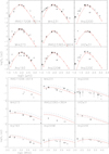 |
Fig. C.1. Low-z starbursts. Crosses mark the observations, and lines show the models. Upper panels: IR SEDs. Lower panels: Radio continuum SEDs. Solid red line: Fiducial model. Dashed red line: Wind model. Dashed blue line: sec+wind model. Dotted blue line: sec+fastwind model. Data points with significantly lower flux densities are due to measurements within smaller apertures. |
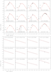 |
Fig. C.2. High-z star-forming galaxies. Crosses mark the observations, and lines show the models. Upper panels: IR SEDs. Lower panels: Radio continuum SEDs. Solid red line: Fiducial model. Dashed red line: Wind model. Dashed blue line: sec+wind model. Dotted blue line: sec+fastwind model. |
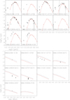 |
Fig. C.6. Submillimeter galaxies. Crosses mark the observations, and lines show the models. Upper panels: IR SEDs. Lower panels: Radio continuum SEDs. Solid red line: Fiducial model. Dashed red line: Wind model. Dashed blue line: sec+wind model. Dotted blue line: sec+fastwind model. |
Appendix D: The influence of different CRe energy loss times on the TIR–radio correlation
TIR-1.4 GHz correlations.
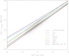 |
Fig. D.1. TIR–1.4 GHz correlation. Gray points: Molnár et al. (2021). Colored lines: Models involving different CRe energy-loss timescales (see Table D.1). |
All Tables
All Figures
|
Fig. 1. Model TIR luminosity as a function of the TIR luminosity derived from observations. The solid line corresponds to the one-to-one correlation. The dotted lines are located at distances of ±0.3 dex from the solid line. |
| In the text | |
|
Fig. 2. Upper panel: model SFR–70 μm correlation. Lower panel: model SFR–TIR correlation. The solid and dotted lines represent an outlier-resistant linear regression and its uncertainty. The dashed line corresponds to a linear correlation. |
| In the text | |
|
Fig. 3. Model median radial profiles of the magnetic field strength (upper panel), CR electron density (middle panel), and free-free optical depth at ν = 1.4 GHz (lower panel) for the four galaxy samples with the associated semi-interquartile ranges. The jumps at R > 10 kpc are caused by taking the median of models with the different radial sizes. |
| In the text | |
|
Fig. 4. Radial profiles of the different median model timescales for the local spirals (left panels) and low-z starbursts (right panels) at ν = 1.4 GHz (upper panels) and ν = 5 GHz (lower panels) with the associated semi-interquartile ranges. |
| In the text | |
|
Fig. 5. Radial profiles of the different median model timescales for the high-z star-forming galaxies (left panels) and high-z starburst galaxies (right panels) at ν = 1.4 GHz (upper panels) and ν = 5 GHz (lower panels) with the associated semi-interquartile ranges. |
| In the text | |
|
Fig. 6. Local spiral galaxies. Crosses mark the observations, and lines show the models. Upper panels: IR SEDs. Data points with significantly lower flux densities are due to measurements within smaller apertures. Lower panels: radio continuum SEDs. Solid red line: Fiducial model. Dashed red line: Wind model. Dashed blue line: sec+wind model. Dotted blue line: sec+fastwind model. |
| In the text | |
|
Fig. 7. Radio continuum SEDs of the low-z starbursts. Solid line: Fiducial model. Dashed line: B = 5.3 × (Σ/10 M⊙ yr−1) μG. Dotted line: |
| In the text | |
|
Fig. 8. Upper left: 70 μm–1.4 GHz correlation. Upper right: 100 μm–1.4 GHz correlation. Lower left: 160 μm–1.4 GHz correlation. Lower right: TIR–1.4 GHz correlation. Colored symbols show model galaxies. Black solid and dotted lines mark the model linear regression. Gray dots show observations. |
| In the text | |
|
Fig. 9. TIR–1.4 GHz correlations. Colored symbols show model galaxies. Black solid and dotted lines show the model linear regression. Upper panel: gray solid and dotted lines show the observed linear regression (Basu et al. 2015). Lower panel: gray error bars show data from Bell (2003). Gray solid and dashed lines mark the observed linear regression (Bell 2003). |
| In the text | |
|
Fig. 10. Upper panel: SFR–1.4 GHz correlation. Lower panel: SFR–150 MHz correlation. Colored lines show observed correlations. Plus symbols mark model galaxies. |
| In the text | |
|
Fig. 11. Calorimeter models. TIR–1.4 GHz correlation. Colored symbols mark the model galaxies, black solid and dotted lines show the model linear regression, and gray dots show observations. |
| In the text | |
|
Fig. 12. Ratios between the magnetic and CR electron energy densities. Upper left: local spiral galaxies. Upper right: low-z starbursts. Lower left: high-z star-forming galaxies. The kink in the radial profiles is caused by the sudden onset of a galactic wind. Lower right: high-z starburst galaxies. |
| In the text | |
|
Fig. C.1. Low-z starbursts. Crosses mark the observations, and lines show the models. Upper panels: IR SEDs. Lower panels: Radio continuum SEDs. Solid red line: Fiducial model. Dashed red line: Wind model. Dashed blue line: sec+wind model. Dotted blue line: sec+fastwind model. Data points with significantly lower flux densities are due to measurements within smaller apertures. |
| In the text | |
|
Fig. C.2. High-z star-forming galaxies. Crosses mark the observations, and lines show the models. Upper panels: IR SEDs. Lower panels: Radio continuum SEDs. Solid red line: Fiducial model. Dashed red line: Wind model. Dashed blue line: sec+wind model. Dotted blue line: sec+fastwind model. |
| In the text | |
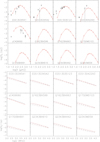 |
Fig. C.3. Same as Fig. C.2. |
| In the text | |
 |
Fig. C.4. Same as Fig. C.2. |
| In the text | |
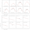 |
Fig. C.5. Same as Fig. C.2. |
| In the text | |
|
Fig. C.6. Submillimeter galaxies. Crosses mark the observations, and lines show the models. Upper panels: IR SEDs. Lower panels: Radio continuum SEDs. Solid red line: Fiducial model. Dashed red line: Wind model. Dashed blue line: sec+wind model. Dotted blue line: sec+fastwind model. |
| In the text | |
|
Fig. D.1. TIR–1.4 GHz correlation. Gray points: Molnár et al. (2021). Colored lines: Models involving different CRe energy-loss timescales (see Table D.1). |
| In the text | |
Current usage metrics show cumulative count of Article Views (full-text article views including HTML views, PDF and ePub downloads, according to the available data) and Abstracts Views on Vision4Press platform.
Data correspond to usage on the plateform after 2015. The current usage metrics is available 48-96 hours after online publication and is updated daily on week days.
Initial download of the metrics may take a while.