| Issue |
A&A
Volume 693, January 2025
|
|
|---|---|---|
| Article Number | A267 | |
| Number of page(s) | 20 | |
| Section | Extragalactic astronomy | |
| DOI | https://doi.org/10.1051/0004-6361/202451607 | |
| Published online | 24 January 2025 | |
Predicting HCN, HCO+, multitransition CO, and dust emission of star-forming galaxies
Extension to luminous infrared galaxies and the role of cosmic-ray ionization
1
Université de Strasbourg, CNRS, Observatoire Astronomique de Strasbourg, UMR 7550, 67000 Strasbourg, France
2
Laboratoire d’astrophysique de Bordeaux, Univ. Bordeaux, CNRS, B18N, allée Geoffroy Saint-Hilaire, 33615 Pessac, France
3
Astronomical Observatory, Jagiellonian University, ul. Orla 171, 30-244 Kraków, Poland
⋆ Corresponding author; This email address is being protected from spambots. You need JavaScript enabled to view it.
Received:
22
July
2024
Accepted:
27
November
2024
Abstract
The specific star formation rate of star-forming main sequence galaxies significantly decreased since z ∼ 1.5 because the molecular gas fraction and star formation efficiency decreased. The gas velocity dispersion decreased within the same redshift range and is apparently correlated with the star formation efficiency (inverse of the molecular gas depletion time). However, the radio–infrared (IR) correlation has not changed significantly since z ∼ 1.5. The theory of turbulent clumpy star-forming gas disks together with the scaling relations of the interstellar medium describes the large- and small-scale properties of galactic gas disks. We extend our previous work on the IR multitransition molecular line, and radio continuum emission of local and high-z star-forming and starburst galaxies to local and z ∼ 0.5 luminous IR galaxies. The model reproduces the IR luminosities, CO, HCN, and HCO+ line luminosities, and the CO spectral line energy distributions of these galaxies. We derived CO(1–0) and HCN(1–0) conversion factors for all galaxy samples. The relation between the star formation rate per unit area and the H2 surface density cannot be fit simply for all redshifts. The star formation efficiency, the product of the gas turbulent velocity dispersion, and the angular velocity of the galaxies are tightly correlated. Galaxies with lower stellar masses can in principle compensate their gas consumption via star formation by radial viscous gas accretion. The limiting stellar mass increases with redshift. The radio continuum emission is directly proportional to the density of cosmic-ray (CR) electrons, but the molecular line emission depends on the CR ionization rate via the gas chemistry. The normalization of the CR ionization rate we found for the different galaxy samples is higher by about a factor of three to five than the normalization for the solar neighborhood. This means that the mean yield of low-energy CR particles for a given star formation rate per unit area is higher by about three to ten times in external galaxies than was observed by Voyager I.
Key words: galaxies: evolution / galaxies: ISM / galaxies: magnetic fields / galaxies: star formation
© The Authors 2025
 Open Access article, published by EDP Sciences, under the terms of the Creative Commons Attribution License (https://creativecommons.org/licenses/by/4.0), which permits unrestricted use, distribution, and reproduction in any medium, provided the original work is properly cited.
This article is published in open access under the Subscribe to Open model. This email address is being protected from spambots. You need JavaScript enabled to view it. to support open access publication.
1. Introduction
The star formation process has changed with time, and a theory of star formation must account for these changes. The density of the cosmic star formation rate (SFR) declined by a factor of approximately ten since the peak at z ∼ 2, which is often referred to as ‘cosmic noon’ (Madau et al. 1998; Hopkins & Beacom 2006). The mean SFR (Ṁ∗) per stellar mass (specific SFR; hereafter sSFR) decreases simultaneously, such that star-forming galaxies form a main sequence in star-formation to stellar mass space (e.g., Brinchmann et al. 2004; Daddi et al. 2007; Elbaz et al. 2007; Noeske et al. 2007a,b; Salim et al. 2007; Whitaker et al. 2012). Galactic starbursts, such as ultraluminous infrared galaxies (ULIRGs) or submillimeter galaxies, represent outliers from the main sequence. The slope and offset of the Ṁ∗–M* main-sequence relation change with redshift (Speagle et al. 2014). The most prominent change is the significant increase in the sSFR (Ṁ∗/M∗) with redshift. Pannella et al. (2015) estimated that the sSFR of a galaxy with M* ∼ 3 × 10¹⁰ M⊙ was six times higher at z = 1 than today. The slope and scatter of this correlation and the evolution of its normalization with cosmic time contain crucial and still poorly known information on galaxy evolution (e.g., Karim et al. 2011; Rodighiero et al. 2011; Wuyts et al. 2011; Sargent et al. 2012).
The gas content of a galaxy largely determines its SFR, but the redshift appears to play a role as well. In local star-forming galaxies, the molecular gas depletion time is correlated with the sSFR (Saintonge et al. 2017). Since z ∼ 1.5, the mean molecular gas fraction (Mmol/M*) decreased by about a factor of four and the molecular gas depletion time, defined as M(H2)/SFR, the inverse of the star formation efficiency (SFE = SFR/M(H2)), increased from shorter than one billion years to about 2 Gyr today (Tacconi et al. 2013, 2020). The high gas velocity dispersion of z ∼ 2 disks is well established (Förster Schreiber & Wuyts 2020). Typical velocity dispersions of the ionized gas are ∼45 km s−1 at z ∼ 2, compared with ∼25 km s−1 at z ∼ 0, and this varies as vturb ∼ 23 + 10z km s−1 (Förster Schreiber & Wuyts 2020). Molecular gas measurements at z > 0 are rare, but follow a similar evolution, albeit with velocity dispersions that are ∼10–15 km s−1 lower (Übler et al. 2019). Weak or no trends are found between the gas velocity dispersion and global galaxy parameters such as M*, SFR, or the SFR surface density (Genzel et al. 2011; Johnson et al. 2018; Übler et al. 2019).
Vollmer et al. (2017; hereafter V17) studied the gas content and associated SFR in main-sequence and starburst galaxies at z = 0 and z ∼ 1–2 in detail. The time-dependent gas chemistry of the turbulent gas clouds was taken into account to produce model IR, CO, HCN, and HCO+ fluxes for comparison with observations. Our relatively simple analytical model appeared to capture the essential physics of clumpy galactic gaseous disks. Most importantly, the model yielded radial profiles of the H2 surface density and the gas velocity dispersion.
There are only few observations of the molecular gas in galaxies during the long period between cosmic noon and now. The Plateau de Bure high-z Blue Sequence Survey 2 (PHIBSS2) sample of luminous infrared galaxies (LIRGs) at z ∼ 0.5 (Freundlich et al. 2019, hereafter F19), which lie within the scatter of the main sequence, provides observations of a large sample during this critical period in the history of the Universe. F19 found a mean molecular gas fraction Mmol/M* = 0.28 ± 0.04 and a depletion time tdep = M(H2)/SFR 0.84 ± 0.07 Gyr compared to the local value of tdep = 2.2 Gyr, with a scatter of 0.3 dex (Leroy et al. 2013). These authors argued that the SFR is mainly driven by the molecular gas fraction (see also Tacconi et al. 2020). The large molecular gas reservoirs fueling star formation are thought to be maintained by a continuous supply of fresh gas from the cosmic web and minor mergers (e.g., Kereš et al. 2005, 2009; Ocvirk et al. 2008; Sancisi et al. 2008; Dekel et al. 2009). However, as shown by the lower tdep in the past, the SFR also varies with redshift. Our model tries to explain (i) the link between the molecular gas depletion time and the gas velocity dispersion and (ii) the evolution of these quantities with redshift.
One of the tightest correlations in astronomy is the relation between the radio continuum (synchrotron) and the far-infrared dust emission (e.g., Yun et al. 2001; Bell 2003; Basu et al. 2015; Molnár et al. 2021). Given the multiple energy-loss mechanisms of cosmic-ray (CR) electrons in galaxies, the tightness of the infrared (IR)–radio continuum correlation is surprising. Vollmer et al. (2022; hereafter V22) extended the analytical model of V17 by including a simplified prescription for the synchrotron emissivity. The magnetic field strength is determined by the equipartition between the turbulent kinetic and the magnetic energy densities. The observed IR-radio correlations for local and high-z SF and starburst galaxies were reproduced by the model within 2σ of the joint uncertainty of model and data for all datasets.
In this work, we extend the models of V17 and V22 to local and z ∼ 0.5 LIRGs to determine whether our model reproduces the radio continuum and molecular line emission of these strongly star-forming galaxies, which fill the gap of model galaxies between 5 × 10¹⁰ (local star-forming galaxies) and 3 × 10¹¹ L⊙ (ULIRGs and high-z star-forming galaxies) in Vollmer et al. (2017; their Fig. 4). The V17 model for the molecular line emission and the V22 model for the radio continuum emission are applied to the extended galaxy sample. The new modeling aspect is the calculation of the CR ionization rate based on the model radio continuum emission, which is calibrated by observations. These ionization rates are used to calculate the molecular abundances (Sect. 2.1.4 in V17). In contrast to V17, the molecular line emission is calculated by RADEX (van der Tak et al. 2007).
The integrated IR, molecular line, and radio continuum emissions of the local and z ∼ 0.5 LIRGs are calculated to confirm our model and study differences (e.g., dust temperature, radio spectral index, and spectral line energy distribution) for different galaxy parameters. The model results for all galaxy samples are used to study the gas supply for star formation by radial accretion within the galactic disks. In addition, the molecular line emission is used to constrain the CR ionization rate. On the one hand, ionization by CR heats the gas, so that the molecular line emission depends on the density of the CR protons and affects the gas chemistry. On the other hand, the radio continuum emission is proportional to the density of the cosmic ray (CR) electrons. The combination of the molecular line emission and radio continuum models thus (i) verifies the validity of our model and (ii) yields the CR ionization rate in external galaxies, which can be compared to the Galactic and local CR ionization rates. Our estimate of the extragalactic CR ionization rates is complementary to those obtained from measurements of HCO+/CO, OH/CO (Gaches et al. 2019; Luo et al. 2023), DCO+/HCO+ (Caselli et al. 1998), HCO+/N2H+ (Ceccarelli et al. 2014), or H3+ (Indriolo et al. 2015; Neufeld & Wolfire 2017).
This article is structured as follows: The galaxy samples are presented in Sect. 2. An important input for the analytic model is the galactic rotation curve. The extraction of these curves for the PHIBSS2 sample is described in Sect. 3. The analytical model of turbulent clumpy star-forming gas disks and their IR, molecular line, and radio continuum emission is described in Sect. 4. The model results are presented in Sect. 5. The molecular gas depletion times, gas viscosity, and accretion rates are discussed in Sects. 6.2 and 6.3. Sect. 6.4 is devoted to the CR ionization fraction. The meaning of the variables used for the model of the gas disk (Sect. 4.1 and Appendix A), the CR ionization rate and molecular abundances (Sect. 4.2), radio continuum and molecular line emission (Sect. 4.3 and Appendix B) are given in Tables C.1, C.2, and C.3, respectively.
2. Galaxy samples
Most galaxies form stars at a rate proportional to their stellar mass. The tight relation between star formation and stellar mass is called the main sequence of star-forming galaxies. It is in place from redshift ∼0 up to ∼4 (e.g., Speagle et al. 2014). Galaxies with much higher SFRs than predicted by the main sequence are called starburst galaxies.
In addition to the four galaxy samples presented in V17 (local and high-z star-forming and starburst galaxies) we included the PHIBSS2 intermediate-redshift (z ∼ 0.5 − 0.8) main-sequence galaxies, which are luminous infrared galaxies (LIRGs; LIR > 1011 L⊙), and local LIRGs that resemble high-z main-sequence galaxies in terms of fmol and σv (DYNAMO; Green et al. 2014; Fisher et al. 2019). Three of our six galaxy samples consist of main-sequence galaxies (local spirals, intermediate-z, and high-z star-forming galaxies), and three are starburst samples (low-z LIRGS and starbursts or ULIRGs, high-z starbursts). High-z and dusty starburst galaxies with SFRs higher than 200 M⊙ yr−1 are called submillimeter (submm) galaxies (e.g., Bothwell et al. 2013). The physical properties of the galaxies are given in Tables B.1 to B.4 of V17.
F19 measured mean fmol and tdep across the main sequence at z ∼ 0.5 to study the connection between star formation and molecular gas and its evolution with redshift. The PHIBSS2 LIRGs naturally fill the luminosity gap between the local main-sequence galaxies and the high-z main-sequence and starburst galaxies. PHIBSS2 represents the first systematic census of molecular gas in this redshift range. Our local LIRG sample is a subset of the DYnamics of Newly Assembled Massive Objects (DYNAMO) survey galaxies (Green et al. 2014), which were identified as disk galaxies and for which CO measurements are available (Fisher et al. 2019). Ten out of 14 galaxies of this sample are LIRGs, and the IR luminosities of the other galaxies are LIR < 1011 L⊙. We added the galaxy IRAS 08339+6517 (Fisher et al. 2022; LIR > 1011 L⊙) to our local LIRG sample. The LIRGs are described in Table D.1 (F19) and the local LIRGs in Table D.2.
3. PHIBSS2 rotation curves
The rotation curve is a crucial model input because it defines the depth of the gravitational potential. For the local star-forming galaxies, we used the parameterized rotation curves of Leroy et al. (2009). For all other galaxy samples except for PHIBSS2, we assumed constant rotation curves.
Since the signal-to-noise ratio of the PHIBSS2 CO observations is quite low, the derived CO line widths are quite uncertain. However, PHIBSS2 has the advantage of providing HST I-band images, which can be converted into a radial mass profile using a constant mass-to-light ratio. In this way, a realistic rotation curve can be obtained. As a cross-check, we produced mock CO spectra based on our model calculations. The line widths of these mock data are consistent with the observed CO line widths. F19 performed single Sérsic fits with galfit (Peng et al. 2002, 2010) on publicly available high-resolution (0.03 arcsec per pixel) HST Advanced Camera for Survey (ACS) images in the F814W I-band. This band is optimal as it is available for all the galaxies of the sample and probes the blue stellar population at z = 0.5–0.8 while avoiding the rest-frame UV light from very young stars. Since we have no additional photometric imaging data, we did not take dust reddening into account. At the PHIBSS2 redshifts, the rest-frame g–r color becomes approximately i–z. The integrated i–z color of the PHIBSS2 galaxies is about g–r ∼ 0.5. According to Fig. 6 of Bell (2003), we expect an uncertainty of about a factor of two on the mass-to-light ratio and thus on the estimate of the mass surface density. Since the inner part of the galaxies, where a bulge might be present, are thought to be redder than the disk, the mass surface density can be underestimated by up to a factor of two there.
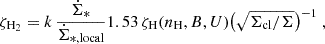
Based on the position of the galaxy center, the inclination, and the position angle obtained by galfit, we produced radial profiles of the I-band surface brightness for each galaxy after masking any sources that did not belong to the galaxy (Fig. 1).
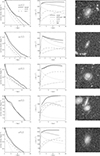 |
Fig. 1. PHIBSS2 stellar surface density profiles and rotation curves. Left panels: Decomposition of the stellar surface density profiles (bulge with a Sérsic index n = 4 and a disk with n = 1). Middle panel: Rotation curve decomposition (bulge, disk, and dark matter). Right panels: HST i-band images (F19) with the galaxy delimited by an ellipse. |
The mass surface density profile was then obtained by normalizing the integral of the Sérsic fit by the total stellar mass obtained by an SED fit (Table D.1). Each profile was further decomposed into two components: a disk component with a Sérsic index of n = 1, and a spherical bulge component with n = 4 (see Section 3.4 of F19). These components were optimized to fit the inner part of the profiles with their high surface density. Finally, we added a dark matter component to obtain flat rotation curves. To do this, the mass ratio of the dark matter halo and the stellar mass content of MDM/M* = 20 was assumed to agree with the findings of Moster et al. (2013), for example. The halo mass profile was determined using the standard description (e.g., van den Bosch 2001). The rotation curve was determined based on the enclosed mass at each distance from the galaxy center. Most of the rotation curves steeply rise in the inner kiloparsec and become flat at radii larger than half the maximum radius.
As a verification, we compared the maximum (model) rotation velocity of the PHIBSS2 galaxies (Fig. 2) with the z = 0 Tully-Fisher relation (e.g., Bell & de Jong 2001; Di Teodoro et al. 2021). For stellar masses lower than M* ∼ 5 × 10¹⁰ M⊙, the relation has the expected slope  (Bell & de Jong 2001). At higher masses, the scatter increases significantly.
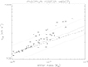 |
Fig. 2. PHIBSS2 galaxies (F19). Maximum rotation velocity as a function of the stellar mass. The dashed and dotted black lines show vrot ∝ M*β with β = 0.22 and 0.25, respectively. The dotted gray lines show a scatter of 0.15 dex (Di Teodoro et al. 2021). |
Fig. 2 shows that 9 of the 59 model PHIBSS2 galaxies have rotation velocities slightly in excess of the Tully-Fisher relation for a dispersion of 0.15 dex (Di Teodoro et al. 2021). These maximum rotation velocities come from the bright compact stellar disks rather than the dark matter (dash-dotted line in Fig. 1). Since the model reproduces the observed CO fluxes reasonably well, these high rotation velocities may well be real.
4. Analytical model
Galactic gas disks are modeled as turbulent clumpy star-forming accretion disks. The turbulent nature of the ISM is taken into account by applying scaling relations for the gas density and velocity dispersion to gas clouds of given sizes. The scaling relations change when the clouds become self-gravitating. The cloud temperature is calculated via the balance of heating and cooling. In this way, the gas density, temperature, and velocity dispersion were determined for each cloud. The molecular abundances depend on the density, temperature, and cosmic-ray ionization rate, which was calculated by using a steady-state model calibrated by the cosmic-ray ionization in the solar neighborhood. The molecular abundances, gas density, velocity dispersion, and temperature served as input for the calculation of the molecular line emission. The radio continuum emission was calculated via a steady-state model calibrated by the observed IR-radio correlations. We performed simulations to predict the emission at many different wavelengths of observed galaxies.
4.1. Gas disk
We used the analytical model described in V17 and Lizée et al. (2022) with a minor modification concerning the self-gravitating gas clouds (see Fig. 2 of V17). This model was also used in V22 to calculate the integrated radio continuum emission of the galaxies. The model considers the warm, cool neutral, and molecular phases of the interstellar medium as a single turbulent gas in vertical hydrostatic equilibrium. The gas is assumed to be clumpy, so that the local density is enhanced relative to the average density of the disk. Using the local density, the freefall time tl, ff of an individual cloud controls the timescale for star formation.
Compared to the version presented in V17, we improved the code by making it modular and permitting the use of RADEX (van der Tak et al. 2007). Since the code now calculates the IR and line emission at a given radius, we set the mass fraction of the self-gravitating clouds with respect to the diffuse clouds (Eq. (7) of V17) y = 0.5 for all galaxies, which is the mean value of all galaxies modeled in V17. We verified that this modification does not change the results by more than ∼30%. In addition, we divided the Toomre parameter Q adopted for the local starburst galaxies in V17 by a factor of two (except for Arp 220E and Arp 220W). This modification led to CO spectral line energy distributions (SLED), which better reproduce the available observations (see Sect. 6.1).
The model simultaneously calculates radial profiles of Σgas, σv, the SFR, and the volume-filling factor, all of which are large-scale properties, and at small scales fmol and the IR SED and molecular line emission. The molecular line emission was calculated via RADEX. For the details of our analytical model, we refer to Appendix A of Lizée et al. (2022). The stellar mass profile is given by the Sérsic fit to the observations, so that the calculations are of the gas distribution and kinematics. The dust was an assumed constant mass fraction (1% of the hydrogen mass).
The rotation curve and the surface density profile of the stellar disk served as model inputs. The model contains three main free parameters: (i) the Toomre parameter Q of the gas, where a Q = 1 disk is a disk with a maximum gas content, (ii) the external accretion rate Ṁ, where an increasing Ṁ at constant Q increases vturb, and (iii) δ = ldriv/lcl (see Appendix C for the meaning of the variables). For each radius R, the model yields the SFR per unit area  , the HI emission, and the IR continuum and molecular line emission for a given set of Q, Ṁ, and δ. Lizée et al. (2022) showed that these radial profiles do not significantly depend on δ for 2 ≤ δ ≤ 10. We thus set δ = 5. The constant that links the rate of energy injection by supernovae to the SFR was set at ξ = 9.2 × 10⁻⁸ (pc yr−1)2 (Eq. (A.5)).
The details of the gas disk model are described in Appendix A.
4.2. Cosmic-ray ionization rate
V17 and Lizée et al. (2022) used a constant CR ionization rate. We calculated the CR ionization rate, which was then injected into the time-dependent gas-grain code Nautilus, which uses the total H2 CR ionization rate ζH2 as input (Wakelam et al. 2012). Cosmic rays with energies above 1 MeV interact with atoms and molecules of the interstellar medium. These high-energy particles can directly ionize a species. This direct process is dominant for H2, H, O, N, He, and CO. Electrons produced in the direct process can cause secondary ionization before they are thermalized. In addition to secondary ionization, the electrons produced in direct cosmic-ray ionization can electronically excite molecular and atomic hydrogen. The radiative relaxation of H2 (and H) produces UV photons that ionize and dissociate molecules. Whereas direct ionization is dominant for CO, secondary ionization and dissociation are dominant for HCN. The CR ionization rate thus affects the chemical abundances.
The spectral particle density of cosmic rays is related to the mean flux or spectrum through
 (1)
(1)
where v(E) is the velocity of a particle with energy E. The ionization rate of hydrogen by cosmic rays is
 (2)
(2)
where ϕs accounts for secondary electrons, and σ(E) is the ionization cross-section. Following Cummings et al. (2016), we set the integration limits to 3 MeV and 107 MeV and ϕs = 0.5. Moreover, we used the Spitzer & Tomasko (1968) formula for the ionization cross-section σ(E).
The CR nucleons (mainly protons) loose energy by the combined effects of ionization and Coulomb losses, adiabatic deceleration, and pion production. To calculate the local (solar neighborhood) CR density spectra of electrons and protons, we followed Pohl (1993). The equilibrium spectrum of CR protons is given by np=
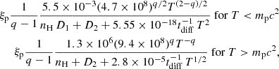 (3)
(3)
where tdiff is the diffusion timescale, D1 = 1 + 0.85 ne/nH, D2 = 1, and q = 2.3 for the CR protons and electrons. Here, T is the kinetic energy, E is the total energy, and T = E for relativistic particles. We used q = 2.3 as expected for superbubbles created by multiple SN remnants (Vieu et al. 2022).
For electrons, ionization and Coulomb losses, non-thermal bremsstrahlung, adiabatic deceleration, inverse Compton losses, and synchrotron emission have to be taken into account (e.g., Lacki et al. 2010). The equilibrium spectrum of CR electrons is given by
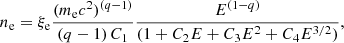 (4)
(4)
with C1 = 4.2 × 10⁷nH, C2 = (8.57 × 10⁻¹⁶ + 6.34 × 10⁻¹⁶) nH, C3 = 6.4 × 10⁻²⁶U + 2.6 × 10⁻²⁵B2, and C4 = 2.2 × 10⁻²⁰, where U is the galactic radiation field. The factors C1 to C4 were adapted to the values used by V22.
For the local ISM, we assumed a density of nH = 0.8 cm−3, a magnetic field strength B = 6 μG (Haverkorn et al. 2015), which is close to the value observed by the voyager spacecrafts (B = 5 μG; Burlaga et al. 2023), a diffusion timescale tdiff = 26 Myr (Lacki et al. 2010), and an electron density ne = 0.1 nH.
The normalization factors of proton and electron spectra, ξp and ξe were chosen such that the observed local CR intensities, averaged over a solid angle, J(E), were recovered. (middle panel of Fig. 3; Cummings et al. 2016; Aguilar et al. 2019). The resulting proton and electron spectra are presented in the upper panel of Fig. 3. The corresponding injection spectra (Eqs. (3) and (4) of Pohl 1993) are shown in the lower panel of Fig. 3. The resulting total number rates of CR electrons and protons are the same, as is often assumed (e.g., Sect. 2 of Pohl 1993).
 |
Fig. 3. Cosmic rays in the solar neighborhood. Upper panel: Model CR particle density spectra. Middle panel: CR energy spectra. The solid black line shows the CR electron model (Pohl 1993), the solid red line shows the CR proton model (Pohl 1993), the solid blue line shows the GALPROP model fit to observations by Cummings et al. (2016), and triangles shows Voyager 1 data (Cummings et al. 2016) and AMS data (Aguilar et al. 2019). Lower panel: CR injection spectra. |
In the solar neighborhood, the CR energy density is ϵCR = ∫n(E) E dE = 0.9 eV cm−3, and that of the magnetic field is also ϵB = 0.9 eV cm−3, following energy equipartition. When we assume that CR ionization of atomic hydrogen due to nuclei with Z > 1 amounts to 1.7 times that due to protons (Cummings et al. 2016), the total CR ionization rate is ζH = 1.6 × 10⁻¹⁷ s−1 (Cummings et al. 2016).
The CR ionization rate was predicted to decrease with the cloud column density (e.g., Padovani et al. 2009). This is because cosmic rays of low energy, which are most effective at ionization, lose all their energy due to ionization losses while traversing high column densities of gas (e.g., Cravens & Dalgarno 1978). Padovani et al. (2022) presented three models for the decrease in the ionization rate with gas column density with ζH2 ∝ N−β, where N is the gas column density and 0.2 ≤ β ≤ 0.6. For simplicity, we adopted an exponent of 0.5.
To calculate the cosmic-ray ionization rate at a given distance R from the center of a galaxy, we set nH to the gas density of the analytical galaxy model (Sect. 4.1), used the interstellar radiation field U and the magnetic field strength of the galaxy model at R, and multiplied ξp and ξe with  of the galaxy model. We further set
  and ζH2 = 2.3/1.5 ζH (Glassgold & Langer 1974). The final expression for the CR ionization rate of molecular hydrogen is
 (5)
(5)
where  is the local Galactic SFR per unit area (Elia et al. 2022). Σcl and Σ are the cloud and disk surface density. The local CR ionization rate (Cummings et al. 2016) corresponds to k = 1.
In our fiducial model, we used a higher CR ionization rate (k = 3) and also calculated a second model with k = 9. k = 9 approximates the value found in the diffuse ISM (AV < 0.3) of the Galaxy (Indriolo et al. 2015; Neufeld & Wolfire 2017).
4.3. Radio continuum emission
As stated in V22, the smallest scale on which the synchrotron–IR correlation holds is approximately the propagation length of CR electrons, which is ≳0.5 kpc at ν = 5 GHz and ≳1 kpc at ν = 1.4 GHz in massive local spiral galaxies (e.g., Tabatabaei et al. 2013; Vollmer et al. 2020). Therefore, only the large-scale part of the gas disk model (Sect. 4.1) was used to calculate the model radio continuum emission.
Following V22, we assumed a stationary CR electron density distribution (∂n/∂t = 0). The CR electrons are transported into the halo through diffusion or advection where they lose their energy via adiabatic losses or where the energy loss through synchrotron emission is so small that the emitted radio continuum emission cannot be detected. Furthermore, we assumed that the source term of CR electrons is proportional to the SFR per unit volume  . For the energy distribution of the CR electrons, the standard assumption is a power law with index q, which leads to a power law of the radio continuum spectrum with index −(q − 1)/2 (e.g., Beck 2015). The details of the radio continuum model are described in Appendix B.
4.4. Molecular abundances and line emission
To determine the chemical abundances, we used seven Nautilus grids for CR ionization rates of (1.3, 3.0, 6.5, 30, 130, 650, 6500)×10−17 s−1 and varied the time, gas density, and gas temperature. The chemical abundances were calculated by interpolating the four-dimensional Nautilus grid with the CR ionization rate of Eq. (5).
The line emission was calculated with RADEX using the inputs as calculated above. The total emission is highly dependent on the gas mass surface densities (and hence filling factors). These come from the local gas densities, and the prescription which decides whether gas is atomic or molecular based on the competition between the molecular formation time and the freefall time. The details are described in Sect. 2.1.1 and 2.4 of V17.
5. Model results
The IR, molecular line, and radio continuum luminosities were calculated with the analytical model presented in the previous section for each of the galaxies of the six samples (local SF galaxies and starbursts, local and z ∼ 0.5 LIRGs, high-z SF galaxies and starbursts). The molecular line emission was calculated by RADEX with input parameters taken from the analytical model. Unlike V17, the CO, HCN, HCO+ abundances were calculated with the variable CR ionization rate given by Eq. (5).
The model input parameters for each galaxy were the stellar surface density profile, the rotation curve, the Toomre Q parameter, and the integrated SFR. All parameters were derived or constrained by observations (Leroy et al. 2009; Downes & Solomon 1998; Genzel et al. 2010; Tacconi et al. 2013; Freundlich et al. 2019; Fisher et al. 2019). We assumed constant rotation curves for the starburst galaxies and the high-z star-forming galaxies. To better reproduce the IR SEDs, we increased the SFRs of the PHIBSS2 galaxies by a factor of 1.5 (Fig. 4). To better reproduce the CO luminosities, we increased the stellar masses by the same factor, which led to an increase in the rotation velocities by a factor of  (Fig. 5). Both factors are within the uncertainties of the observational estimates via SED fitting (0.3 dex for the mass estimate; Roediger & Courteau 2015) and combined UV and IR luminosities (0.2 dex for the SFR; Leroy et al. 2009). The use of a starburst attenuation law in the SED fitting can indeed underestimate the galaxy mass (e.g., Buat et al. 2019). For internal consistency, the PHIBSS stellar masses were also increased by a factor of 1.5.
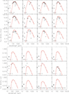 |
Fig. 4. Infrared spectral energy distributions. Red pluses and solid line: model SED. Red dashed line: modified Planck fit for temperature determination. Black crosses: VizieR photometry. The errors bars are shown, if present in the VizieR tables, but often barely visible. Upper panel: z ∼ 0.5 LIRGs. Lower panel: local LIRGs. |
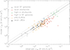 |
Fig. 5. Model CO luminosities as a function of the observed CO luminosities. The model CO transition corresponds to the observed transition. The lines correspond to the one-to-one relation with a scatter of a factor of two. |
5.1. Metallicity, dust SED, TIR luminosity, and dust temperature
Following V17, our leaky-box model used an effective yield, meaning that enriched gas can escape and be accreted from the circumgalactic medium. This led to a gas metallicity of
 (6)
(6)
with
 (7)
(7)
This avoided a severe underestimation of the metallicities of the ULIRG and high-z star-forming galaxy samples. The oxygen abundance was then 12+log(O/H) = log(Z/Z⊙)+8.7, with 12+log(O/H) = 8.7 being the solar oxygen abundance (Asplund et al. 2005).
Fig. 6 shows the metallicity distributions of our samples, with excellent agreement with V17 and observations for the local and high-z SF galaxies. However, the model metallicities of half of the starburst galaxies show metallicities that are two to four times higher than observed. The mean model metallicity of the local LIRGs is 12+log(O/H) = 9.0 ± 0.2, which is very close to the mean value of six DYNAMO galaxies of 12 + log(O/H) ∼ 9.1 (Lenkić et al. 2021). The mean model metallicity of the z ∼ 0.5 LIRGs is roughly solar, 12+log(O/H) = 8.6 ± 0.2. This is lower by about a factor of two than the mean gas metallicity found for 0.5 ≤ z ≤ 0.7 galaxies with a comparable stellar mass and sSFRs 12 + log(O/H)∼8.9; Guo et al. 2016).
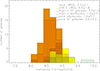 |
Fig. 6. Distribution of galaxy metallicities. The solid black line shows the local SF galaxies. The dotted blue line shows local starbursts. The dashed green line shows high-z starbursts. The dash-dotted red line shows high-z SF galaxies. The yellow line shows local LIRGs. The orange line shows z ∼ 0.5 LIRGs. The solar metallicity is assumed to be 12+log(O/H) = 8.7. |
Following V17, we extracted all available photometric data points for our galaxy samples from the CDS VizieR database1 for a direct comparison between the model and the observed dust SED. Since the flux densities were determined within different apertures, we only took the highest flux densities for a given wavelength range around a central wavelength λ0 (0.75 ≤ λ/λ0 ≤ 1.25). In this way, only the outer envelope of the flux density distribution was selected. Since our dust model does not include stochastically heated small grains and PAHs, the observed IR flux densities for λ ≲ 50 μm cannot be reproduced by the model.
We assumed a dust mass absorption coefficient of the following form:
 (8)
(8)
with λ0 = 250 μm, κ0 = 0.48 m2kg−1 (Dale et al. 2012), and a gas-to-dust ratio of  (including helium; Rémy-Ruyer et al. 2014). The exponent was β = 2 for the starburst galaxies and β = 1.5 for the star-forming galaxies and LIRGs.
The model dust IR SEDs of the local and z ∼ 0.5 LIRGs are presented in Fig. 4 and Figs. D.12 to D.14.
Infrared flux densities at λ > 100 μm are only available for two DYNAMO galaxies and IRAS 08339+6517 (local LIRGs). For these three galaxies, the models reproduce the observations very well. More data are available for the PHIBSS2 galaxies (z ∼ 0.5 LIRGs), and the model dust IR SEDs reproduce the observations. For 80% of the model galaxies, the fluxes are close to the observed values. For 8 out of 59 galaxies, the peak model flux is higher by a factor of two than the observed SED, and for two galaxies, it is lower by a factor of two.
The model and observed 10 μm to 1000 μm luminosities (hereafter TIR) are presented in the upper panel of Fig. 7. The TIR luminosities of the DYNAMO and PHIBSS2 galaxies were estimated by LTIR = 1010×SFR (Calzetti 2013). The model and observed TIR luminosities agree within a factor of two. The model local LIRGs are slightly underestimated, and z ∼ 0.5 LIRGs are slightly overestimated (see the upper panel of Fig. 7).
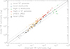 |
Fig. 7. Model total IR luminosity as a function of the observed TIR luminosity of the galaxies. The lines correspond to an outlier-resistant linear bisector fit and its dispersion. |
We fit modified Planck functions with β = 1.5 to the model dust IR SEDs to derive the dust temperatures. The modified Planck functions are shown as dashed red lines in Fig. 4 and Figs. D.12 to D.14. The resulting distributions of the dust temperatures for the different galaxy samples are presented in Fig. 8. The dust temperatures of the local and z ∼ 0.5 LIRGs lie between 20 K and 30 K, with a mean of 27 K for both samples. This is intermediate between those of the local and high-z SF galaxies.
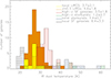 |
Fig. 8. Model distribution of dust temperatures. Black solid line: local SF galaxies. Blue dotted line: local starbursts. Green dashed line: high-z starbursts. Red dash-dotted line: high-z SF galaxies. Yellow: local LIRGs. Orange: z ∼ 0.5 LIRGs. |
5.2. Integrated CO, HCN(1 − 0), and HCO+(1 − 0) fluxes
The model and observed CO luminosities are shown in Fig. 5: CO(2–1) for the local SF galaxies and LIRGs, CO(1–0) for local LIRGs and starbursts, and CO(3–2) for all high-z galaxies. The transitions vary due to instruments and source redshifts. The use of a nonconstant ionization rate changes the CO emission, such that LCO for high-z SF galaxies is ∼50% lower and 50% higher for high-z starbursts than in V17. The effect is weaker at low redshift.
The model and observed LTIR–LHCN relations are compared in Fig. 9. The model LHCN of the local galaxies agree with those in V17, but the high-z galaxies are higher by factor of 1.5 to 2 than in V17, primarily due to the variable CR rate (Eq. 5). The model LTIR–LHCN relations of the local SF and LIRGs and that of most z ∼ 0.5 galaxies are higher by a factor of two than observed. The low model LHCN of high-z starburst galaxies is consistent with the results of Rybak et al. (2022), who only detected one out of six z ∼ 3 starburst galaxies in the HCN(1–0) line. The model LHCN of the local starbursts is broadly consistent with observations (upper panel of Fig. 10). Furthermore, the HCO+(1–0) luminosities of the local starbursts are fully consistent with observations (lower panel of Fig. 10).
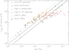 |
Fig. 9. Model HCN(1–0) luminosities as a function of the model TIR luminosities. The upper solid line corresponds to L′HCN/LTIR = 980 (Jiménez-Donaire et al. 2019), and the dashed lines are offset by a factor of 0.5 and 2. The lower solid line corresponds to a 2.3 lower L′HCN/LTIR as found for luminous IR galaxies by García-Burillo et al. (2012). |
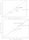 |
Fig. 10. Model HCN(1–0) (upper panel) and HCO+(1-0) (lower panel) luminosity as a function of the observed HCN(1–0)/HCO+(1-0) luminosity (Graciá-Carpio et al. 2008). The solid line corresponds to the one-to-one relation, and the dotted lines show a dispersion of 0.3 dex. The dashed lines correspond to a robust bisector fit. |
The new model, with a CR ionization rate calculated rather than injected, yields results as good (within less than a factor of two) as V17 and has the advantage of revealing in which type of galaxy the CR ionization rate significantly modifies the molecular line emission. For example, the model CO luminosities of the high-z SFR galaxies are lower by about 50%, whereas those of the high-z starbursts are higher by about 50% than those obtained by V17. Whereas the agreement between the model and observed CO luminosities becomes somewhat worse for the high-z star-forming galaxies, it becomes somewhat better for the high-z starbursts. V17 assumed a constant value of the CR ionization rate for each galaxy sample. A high CR ionization rate has the effect of a high direct ionization of CO (see Sect. 4.2) and thus a decrease in the CO abundance and line flux. It thus appears that V17 under- and overestimated the CR ionization rate in the high-z SFR galaxies and starbursts, respectively.
5.3. CO spectral line energy distributions
The CO SLEDs normalized to the CO(1–0) and CO(2–1) fluxes (expressed in Jy km s−1) are presented in Fig. 11.
 |
Fig. 11. Mean model CO SLEDs of our galaxy samples. The dotted line corresponds to a constant brightness temperature. The high-z SF galaxy sample was divided into a z ∼ 1.5 (solid red) and a z > 2 (dashed red) subsample. IRAS 08339+6517 is shown by the dashed black line. |
For the inner Milky Way, the new mean model CO SLED reproduces the CO(3–2)/CO(2–1) line ratio (Fixsen et al. 1999) better than V17. Kamenetzky et al. (2016) observed Jupper > 6 transitions of CO in galaxies with TIR luminosities from 3 × 10¹¹ to 1012 L⊙ and LTIR > 1012 L⊙, which are shown with model ULIRG CO SLEDs in Fig. 12. The high-J transitions have higher luminosities than observed, as in V17, although the shapes of the CO SLEDs are comparable. The model and observed CO SLEDS of five local ULIRGs (Rosenberg et al. 2015) are shown in the upper panel of Fig. 12. The CO(5–4) luminosities are well reproduced, and the higher CO transitions are reproduced within a factor of two, except for Mrk 231, for which they are overestimated. The lower transitions were not observed by Kamenetzky et al. (2016).
 |
Fig. 12. CO SLEDs of local starburst galaxies (ULIRGs). Upper panel: the black boxes linked by black lines represent the observed mean CO SLEDs of ULIRGs with total IR luminosities between 3 × 10¹¹ and 1012 L⊙ and higher than 1012 L⊙, respectively (from Kamenetzky et al. 2016). Lower panels: model (pluses) and observed CO SLEDs (Rosenberg et al. 2015; triangles). |
The CO model SLEDs of the high-z SF galaxies can be compared to the results of Boogaard et al. (2020) for z ∼ 1.5 and Valentino et al. (2020) for z > 2. The maximum of the mean CO SLED is observed at Jup = 5 at z ∼ 1.5 and Jup = 7 at z ∼ 2.5. As in V17, the maximum of the model CO SLED is found at Jup = 4 at z ∼ 1.5 and Jup = 5 at z > 2. The model CO SLEDs normalized to the CO(1–0) and CO(2–1) fluxes are compatible with the available observations. The mean model CO SLEDs of LIRGs are identical within 1σ, and the mean model SLED normalized to CO(1–0) is consistent with the observations of five DYNAMO galaxies by Lenkić et al. (2021).
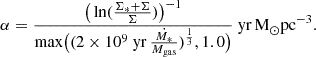
5.4. Integrated CO and HCN conversion factors
Since the integrated H2 mass and the line emission were calculated within the model (V17), the integrated mass-to-light conversion factors can be determined (Fig. 13).
 |
Fig. 13. CO(1–0) conversion factors for our galaxy samples in units of M⊙(K km s−1pc2)−1. |
The mean model conversion factor of local spirals (⟨αCO(1 − 0)⟩ = 6.4 ± 3.3 M⊙(K km s−1pc2)−1) is higher than but consistent within 1σ with the commonly used value of αCO(1 − 0) = 4.3 M⊙(K km s−1pc2)−1 (Bolatto et al. 2013, Chiang et al. 2024).
The mean conversion factor of the local and high-redshift starburst galaxies (⟨αCO⟩∼1.3 ± 0.4 M⊙(K km s−1pc2)−1) is about twice that of observed high-z starburst galaxies (αCO = 0.8 M⊙(K km s−1pc2)−1 (Downes & Solomon 1998). The model αCO(1 − 0) of high-z star-forming galaxies is ⟨αCO⟩ = 3.5 ± 1.8 M⊙(K km s−1pc2)−1, which is close to the ⟨αCO⟩ = 3.7 ± 2.1 M⊙(K km s−1pc2)−1 for the LIRGs, regardless of redshift, and it is similar to the standard MW value.
The HCN conversion factor is usually interpreted as the HCN(1–0) flux (K km s−1) divided by the column density of dense gas (n ≥ 3 × 104 cm−3; e.g., Gao & Solomon 2004), or equivalently, the ratio of the HCN luminosity (K km s−1pc2) to the dense gas mass (upper panel of Fig. 14). In addition, the HCN(1–0)–MH2 conversion factor (lower panel of Fig. 14) might also be a useful quantity. The canonical HCN(1–0)–dense gas conversion factor is αHCN = 10 M⊙(K km s−1pc−1)−1 (Gao & Solomon 2004).
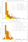 |
Fig. 14. HCN conversion factors in units of M⊙(K km s−1pc2)−1. Upper panel: HCN(1–0)–dense gas conversion factors; lower panel: HCN(1-0)–MH2 conversion factors for our galaxy samples. |
The model HCN(1–0)–dense gas conversion factors of the local and high-z star-forming and starburst galaxies are consistent with the canonical value. The HCN conversion factors of the local and z ∼ 0.5 LIRGs are lower by about a factor of two than those of local and high-z star-forming and starburst galaxies.
Whereas the HCN(1-0)–MH2 conversion factors of the local and high-z starbursts and high-z SF galaxies are consistent within 1σ with those given by V17, the HCN conversion factor of the local SF galaxies is twice that of V17. Interestingly, the conversion factors of the local and z ∼ 0.5 LIRGs are about the same and close to that of the high-z starbursts.
5.5. Integrated radio continuum emission
The model radio continuum emission at 150 MHz and 1.4 GHz was calculated using the framework presented in Sect. 4.3. The monochromatic (70, 100, 160 μm) and TIR–radio correlations of all six samples are shown in Fig. 15. The radio continuum luminosities at 1.4 GHz are consistent with those of V22, except for the high-z starburst galaxies, whose radio luminosities are about twice those of V22. The difference is caused by the different exponent of the CR energy distribution (Eq. (B.1) with q = 2.3 instead of q = 2 in V22). The local and z ∼ 0.5 LIRGs nicely fall on and complement the correlations of the other galaxy samples that were highlighted by V17.
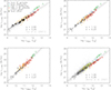 |
Fig. 15. IR-radio correlations. Upper left: 70 μm – 1.4 GHz correlation. Upper right: 100 μm – 1.4 GHz correlation. Lower left: 160 μm – 1.4 GHz correlation. Lower right: TIR – 1.4 GHz correlation. The colored and black symbols show model galaxies. For clarity, the z ∼ 0.5 LIRGs are shown as yellow diamonds in the lower right panel. The solid and dotted black lines mark the model linear regression. The gray dots show the observations. |
We calculated the slopes and offsets of the correlation using an outlier-resistant bisector fit. The results together with the correlation scatter are shown in Fig. 15. Furthermore, we used a Bayesian approach to linear regression with errors in both directions (Kelly 2007). We assumed uncertainties on the TIR and radio luminosities of 0.2 dex for the local galaxies and 0.3 dex for the high-z galaxies.
In agreement with V22, the exponents derived from the bisector fits of the monochromatic IR–radio correlations increase with increasing wavelength from 0.94 at 70 μm to 1.12 at 100 μm and to 1.41 at 160 μm. The exponent of the TIR–radio correlation is 1.06. These slopes are consistent with those derived with a Bayesian approach, the uncertainties of which are about 0.04.
Beck (2015) studied the radio–TIR correlation in star-forming galaxies chosen from the PRism MUltiobject Survey up to redshift 1.2 in the XMM-LSS field, employing the technique of image stacking. These authors found an exponent of the TIR–1.4 GHz correlation of 1.11 ± 0.04. The lower panel of Fig. 16 shows the direct comparison between our model galaxies (local and high-redshift galaxies) and those of Beck (2015). The model and data show comparable exponents and scatters.
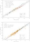 |
Fig. 16. TIR–1.4 GHz correlations. The symbols show the model galaxies. Black solid and dotted lines show the model linear regression. Upper panel: Gray solid and dashed lines show the observed linear regression (Beck 2015). Lower panel: Orange error bars show data from Bell (2003). Gray solid and dashed lines mark the observed linear regression (Bell 2003). |
(Bell 2003) assembled a diverse sample of local galaxies from the literature with FUV, optical, IR, and radio luminosities. They found a nearly linear radio–IR correlation. The upper panel of Fig. 16 shows the direct comparison between our local model galaxies (spirals and low-z starbursts) and the compilation of Bell (2003). The slopes agree within 1σ and between the offsets within 0.4σ of the joint uncertainty of model and data.
The resulting correlations between the 1.4 GHz/150 MHz luminosity and the SFR are presented in Fig. 17. The model slopes of the log-log correlation are 1.07 ± 0.04 at 1.4 GHz and 1.05 ± 0.05 at 150 MHz. Both correlations are thus slightly superlinear. Whereas the slope of the 1.4 GHz correlation is consistent with the correlation reported by V17, the slope of the 150 MHz correlation is slightly higher than that obtained by V17. The two model correlations are consistent with existing estimates based on observations (Fig. 17).
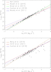 |
Fig. 17. Upper panel: SFR–1.4 GHz correlation. Lower panel: SFR–150 MHz correlation. The colored lines show observed correlations. The pluses mark the model galaxies. The dashed black lines in both panels correspond to outlier-resistant linear bisector fits. |
6. Discussion
Our modeling of the six galaxy samples at different redshifts reproduced the available observations within a factor of two. The principal open parameter of the large-scale model of the turbulent star-forming galactic disk is the Toomre parameter, which is expected to be not much higher than unity. The influence of the Toomre parameter Q on the molecular line emission of the local starburst galaxies is discussed in Sect. 6.1.
The model yields the gas mass, velocity dispersion, the turbulent driving length scale, and the gas viscosity ν = vturbldriv. The resulting star formation efficiencies are discussed with respect to the gas velocity dispersion in Sect. 6.2. The radial gas transport within the galactic disks via the turbulent gas viscosity is discussed in Sect. 6.3.
6.1. Effect of the Toomre Q parameter
To investigate the effect of the Toomre Q parameter on the CO SLEDs of the local starburst galaxies, we increased Q by factors of 1.5, 2, 2, 2, and 1.5. The resulting CO SLEDs are presented in Fig. 18. The comparison with Fig. 12 shows that a higher Q leads to a significantly steeper CO SLED. We interpret this behavior as being caused by an increased gas velocity dispersion with increasing Q. The higher velocity dispersion leads to a higher turbulent heating, and thus, to higher gas temperatures. The high gas temperature in turn leads to higher brightness temperatures of the high-J CO transitions. The agreement between the model and observed SLEDs with higher values of Q is much worse than that of the fiducial values (Fig. 12). This strongly supports that the values of Q in local starburst galaxies are low.
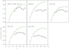 |
Fig. 18. CO SLEDs of the local starburst galaxies with 1.5 to two times higher Q values compared to Fig. 12. Black triangles: Rosenberg et al. (2015). Green lines: models. |
6.2. Molecular gas depletion time and gas velocity dispersion
Within our analytical model, the only energy source for turbulence is stellar feedback (Sect. 4). As stated in Sect. 4.1, our star formation prescription leads to an SFR per unit area, which is proportional to the gas pressure (Fig. A.1), as is expected if star formation is pressure-regulated and feedback-modulated (Ostriker & Kim 2022). Since our model reproduces the molecular line and radio continuum emission of the six galaxy samples, we conclude that the energy injection via stellar feedback is sufficient to maintain the observed level of turbulence in these galaxies.
The ΣSFR − ΣH2 correlation of our model galaxies is presented in the upper panel of Fig. 19. For the area calculation, the stellar scale length was adopted. The log-log relation cannot be fit with a single slope or offset. Despite similar ΣH2, the local LIRG SFRs are higher by up to about five times than the local SF galaxies. Perhaps surprisingly, the local and high-z starbursts and the local and z ∼ 0.5 LIRGs have comparable star formation efficiencies. The slopes of the log(ΣSFR)−log(ΣH2) correlation are 1.2, 1.7, 2.0, 1.1, 1.4, and 2.3 for local SF galaxies and starbursts, local and z ∼ 0.5 LIRGs, and high-z SF galaxies and starbursts, respectively (as derived by the IDL routine robust_linefit). Only the local and high-z starbursts and the local LIRGs show slopes higher than 1.5. We interpret these steep slopes as a result of the compactness of these galaxies. Small galaxy sizes lead to deep potential wells, short dynamical times, and high gas densities.
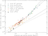 |
Fig. 19. Star formation rate per unit area as a function of the molecular gas surface density. The dotted lines show linear and square fits to guide the eye. The dashed lines show robust fits to the different galaxy samples. |
The molecular gas depletion time as a function of the sSFR of the model galaxies is presented in the upper panel of Fig. 20. The slope of the log-log relation is −0.61, and the scatter is 0.12 dex. The local and high-z starbursts show by far the largest scatter. The slope of the observed log-log relation (−0.56; Saintonge et al. 2017; middle panel of Fig. 20) is consistent with that of the model relation. The observed scatter is larger by a factor of two than the model scatter. We conclude that the tight observed tdep, H2–sSFR relation is well reproduced by the SF galaxy models. The molecular gas depletion time as a function of redshift is presented in the lower panel of Fig. 20). The depletion time decreases with redshift as (1 + z)−0.58 up to z ∼ 1.5 and seems to become constant for z ≳ 2. The exponent of −0.58 is consistent with that found by Tacconi et al. (2018) for galaxies at z < 0.7 (−0.62; their Fig. 4).
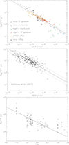 |
Fig. 20. Molecular gas depletion time. Upper panel: as a function of the sSFR for the model galaxies. Middle panel: as a function of the sSFR for the observations from Saintonge et al. (2017). Lower panel: as a function of redshift for the model galaxies. The lines correspond to an outlier-resistant linear bisector fit and its dispersion. |
Silk (1997) suggested that the SFR and the gas mass are related by the dynamical time: SFE∝Ω−1. This relation with respect to the molecular gas is shown in the upper panel of Fig. 21. The slope of the log-log relation is 1.1. The Ω dependence captures the difference between the SF galaxies and starbursts. However, the scatter of 0.4 is quite large and the z ∼ 0.5 LIRGs do not follow the relation. The log(SFE)−log(Vturb) relation has a slope of 1.3 and is considerably tighter (0.20 dex; see also Fisher et al. 2019). Only the starburst galaxies do not follow this relation.
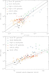 |
Fig. 21. Star formation efficiency. Upper panel: Star formation efficiency with respect to the molecular gas as a function of the angular velocity Ω. The lines correspond to an outlier-resistant linear bisector fit and its dispersion. Lower panel: Star formation efficiency with respect to the molecular gas as a function of the turbulent velocity dispersion. The fit only applies to the SF galaxies. |
The turbulent velocity dispersion increases with the SFR, the SFR per unit area, and the gas fraction (Fig. 22). However, the scatter of these trends is large. The relation between the velocity dispersion and the gas fraction of the SF galaxies has a scatter of 0.4 dex (see also Girard et al. 2021). The slope of the log-log relation is unity.
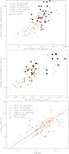 |
Fig. 22. Model turbulent velocity as a function of the SFR (upper panel), the SFR per unit area (middle panel), and the gas fraction (lower panel). The filled circles and boxes correspond to observed values (Downes & Solomon 1998; Cresci et al. 2009; Tacconi et al. 2013; Girard et al. 2021; Nestor Shachar et al. 2023). The lines correspond to an outlier-resistant linear bisector fit and its dispersion. |
The log(SFE)−log(vturbΩ) correlation for the starburst galaxies yields the lowest scatter (0.21 dex) The slope is 0.87 (see lower panel of Fig. 23). The reason for this behavior is the star formation prescription  (Eq. (A.4)). With H ∼ vturbΩ−1, we obtain
  . With
  (upper panel of Fig. 23), we obtain the almost linear relation between the SFE and (vturb × Ω).
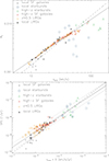 |
Fig. 23. Upper panel: Inverse of the overdensity of selfgravitating clouds as a function of the turbulent velocity dispersion. The solid line corresponds to an outlier-resistant linear bisector fit, and the dashed line shows ΦV = vturb/(1 km s−1)/7000. Lower panel: Star formation efficiency with respect to the molecular gas as function of (vturb × Ω). The solid and dotted lines correspond to an outlier-resistant linear bisector fit and its dispersion. The dashed line corresponds to SFE = 10−3 vturbΩ. |
6.3. Gas viscosity
The turbulent viscosity of the gas is given by ν = vturb ldriv. To investigate the importance of radial gas accretion with respect to the SFR, we evaluated the star formation timescale ( ) and the viscous timescale (tvisc = R2/ν) at the effective radius of each galaxy. Fig. 24 shows the model tvisc/t* ratio versus stellar mass for the SF galaxies (top) and starbursts (bottom). Most starburst galaxies have tvisc/t* ≤ 2, which means that the radial gas transport can approximately compensate for the mass loss via star formation.
 |
Fig. 24. Fraction tvisc/t* as a function of the stellar mass of the model galaxies. Upper panel: SF galaxies. The tvisc/t* fractions of the star-forming galaxies should thus be taken as lower limits with an uncertainty of a factor of two towards higher values. The dashed lines are observed trends with stellar mass. Lower panel: Starburst galaxies. |
The situation is different for the SF galaxies (upper panel of Fig. 24). Only a minority of the SF galaxies have tvisc/t* ≤ 2. The direct comparison with the spatially resolved models of the local SF galaxies (Lizée et al. 2022) shows that our tvisc/t* fractions can be underestimated by up to a factor of three. The tvisc/t* fractions of the star-forming galaxies should thus be taken as lower limits with an uncertainty of a factor of two toward higher values. Our conclusions are not significantly affected by this uncertainty. A trend appears where tvisc/t* increases with stellar mass, such that replenishment becomes more difficult at high mass, at least at the effective radius (see also Vollmer & Leroy 2011). Robust bisector fits of the log-log relations lead to slopes of 1.2 for the local starbursts and LIRGs, 1.5 for the z ∼ 0.5 LIRGs, and 1.3 for the high-z SF galaxies. The trends with a log-log slope of 1.4 are shown as dashed lines in the upper panel of Fig. 24. In addition, there seems to be an offset related to redshift. The lines cross tvisc/t* = 2 at higher stellar masses for increasing redshift: M(z = 0)∼2 × 10¹⁰ M⊙, M(z = 0.5)∼4 × 10¹⁰ M⊙, and M(z = 1.5)∼8 × 10¹⁰ M⊙. They cross tvisc/t* = 1 at M(z = 0)∼1 × 10¹⁰ M⊙, M(z = 0.5)∼2 × 10¹⁰ M⊙, and M(z = 1.5)∼5 × 10¹⁰ M⊙. This means that galaxies below these limiting masses can in principle compensate for their gas consumption via star formation by radial viscous gas accretion.
6.4. Cosmic-ray ionization rate
There is a discrepancy of about a factor of ten between the measurements of low-energy cosmic rays by Voyager 1 in the solar neighborhood (ζH ∼ 2 10−17 s−1; Cummings et al. 2016) and the astronomical inferences toward many lines of sight and at several galactocentric radii (ζH ∼ 2 10−16 s−1, e.g., Indriolo et al. 2015, Neufeld & Wolfire 2017). New estimates of the gas density in diffuse molecular clouds led to a significantly smaller discrepancy (a factor of ∼3; Obolentseva et al. 2024). As described in Sect. 4.2, the CR ionization fraction was calculated for a given gas density, radiation field, and magnetic field strength. The only free parameter was the overall normalization of the CR ionization rate (parameter k in Eq. (5)). For k = 1, the CR ionization rate measured in the solar neighborhood was recovered for the conditions of the local ISM. In the following, we estimate k based on the molecular line emission and radio continuum emission.
The molecular line emission depends on the CR ionization rate, which is taken into account by Nautilus. In all previous sections, we showed the results for k = 3, which led to results closest to the available molecular line and radio continuum observations. Motivated by the observed CR ionization rate at several galactocentric radii, we set k = 9. In this case, the CO(1–0) and HCN(1–0) fluxes are significantly lower than observed (Fig. 25). The k = 9 model can thus be discarded.
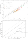 |
Fig. 25. Models with k = 9 instead of k = 3. Upper panel: Model CO flux of the galaxies of the different samples as a function of the observed CO flux. Lower panel: Model HCN(1–0) flux as a function of the observed HCN(1–0) flux for the local starburst galaxies. |
The question now is whether ζH really varies with NH (Eq. (5)). We calculated the k = 3 model without the NH dependence on ζH, and the CO(1–0) and HCN(1–0) fluxes became significantly lower than observed (Fig. 26). We conclude that ζH indeed varies with NH.
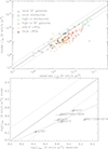 |
Fig. 26. Models without the dependence of ζH on the gas column density. Upper panel: Model CO flux of the galaxies of the different samples as a function of the observed CO flux. Lower panel: Model HCN(1–0) flux as a function of the observed HCN(1–0) flux for the local starburst galaxies. |
On the other hand, the density of the CR electrons can be calculated from the radio continuum model (Sect. 4.3). Cosmic-ray electrons with energy E emit most of their energy at the frequency νs (e.g., Eq. (5) of V22), where
 (9)
(9)
with E = γm0c2 for high Lorentz factors γ. The Lorentz factor of electrons emitting at 1.4 GHz γ1.4 was calculated by inverting Eq. (9). The CR electron density at a frequency of 1.4 GHz was then calculated using Eq. (B.13) with the model spectral index α12 calculated between 1 and 2 GHz,
 (10)
(10)
To normalize the CR electron density at 1.4 GHz to that based on the normalization found in the solar neighborhood, we used Eq. (4) evaluated at the energy corresponding to an emission frequency of 1.4 GHz (Eq. (9)) (ne, neighborhood) with the ISM conditions from the analytical model (Sect. 4.2). The final overdensity of CR electrons is  . Consistent results were found for frequencies of 15 and 150 MHz.
The visual inspection of the corresponding radial profiles  showed variations typically with a decreasing
  with increasing radius. We calculated the mean of all
  for the different galaxy samples. The results are presented in Table 1.
Overdensity of CR electrons with respect to the solar neighborhood.
The overdensities of CR electrons with respect to the solar neighborhood range between 2 and 10. Based on Eq. (1), we assumed that  .
.
The mean of  from the radio continuum observations is about 4–5. This compares well to the value of k = 3 found from the molecular line emission. We thus conclude that the normalization of the CR ionization rate found for the different galaxy samples is higher by about a factor of three to five than the normalization for the solar neighborhood. The mean yield of low-energy CR particles for a given SFR per unit area is thus higher by about three to five times in external galaxies than the yield in the solar neighborhood. This is two to three times less than the discrepancy of a factor of ten between measurements of low-energy cosmic rays by Voyager 1 in the solar neighborhood and the astronomical inferences toward many lines of sight and at several galactocentric radii. It agrees well with the recent measurements of Obolentseva et al. (2024). Given the large uncertainties of the measured CR ionization rates (Dalgarno 2006), the two findings are broadly consistent. It seems thus that the low-energy CR particles found in the solar neighborhood by Voyager 1 are underabundant by about a factor of 5 ± 4 with respect to the mean at the solar radius. We can only speculate that this is caused by the 3D geometry of the magnetic field in the Local Bubble (Alves et al. 2018), leading to an increased escape of CR particles and/or preventing them from entering the solar neighborhood.
7. Summary and conclusions
The theory of turbulent clumpy star-forming gas disks (Vollmer & Beckert 2003) provides the large- and small-scale properties of galactic gas disks. Within this model, stellar feedback provides the energy injection to maintain turbulence. Stars are formed according to  (Eq. (A.4)), where the inverse of the overdensity of self-gravitating clouds ΦV is proportional to the gas velocity dispersion vturb (upper panel of Fig. 23). This prescription leads to a SFR per unit area that is proportional to the gas pressure (Fig. A.1), as is expected if star formation is regulated by pressure and modulated by feedback (Ostriker & Kim 2022). Moreover, the radially averaged star formation efficiencies per freefall time range between 0.004 and 0.075, which is broadly within the range of the canonical value of ϵff ∼ 0.01 (Krumholz et al. 2012).
We extended the work of V17 on local and high-z SF and starburst galaxies by (i) adding local and z ∼ 0.5 LIRG samples, (ii) including RADEX, and (iii) adding a CR ionization fraction that was proportional to the star formation surface density (Eq. (5)). These newly added galaxy samples fill the gap in total IR luminosity between the local and high-z SF galaxies well. The gas chemistry computed by the Nautilus code depends on the CR ionization rate, which was calculated following the analytical model of Pohl (1993) using the local density, magnetic field strength, and radiation field of our analytical model. The injection rate of CR particles is proportional to the SFR per unit area (Eq. (5)). In the current version of the code, the molecular line emission is calculated by RADEX. The model reproduces the IR luminosities, CO, HCN, and HCO+ line luminosities, and the CO SLEDs of the LIRGs (Figs. 4 to 12). We derived the model CO(1–0) and HCN(1–0) conversion factors for all galaxy samples (Figs. 13 and 14).
Since the model yields the H2 masses, the relation between the star formation per unit area and H2 surface density (Kennicutt-Schmidt law) can be established. The log-log relation cannot be fit with a single line or a single offset (Fig. 19). As observed, the SFE varies linearly with the sSFR (Fig. 20). Moreover, the log(SFE)–log(vturb) relation has a small scatter of 0.20 dex with an exponent of 1.3 (lower panel of Fig. 21). The reason for this behavior is that the ΦV is approximately proportional to vturb (upper panel of Fig. 23). The lowest scatter of 0.21 dex for the sample including the starburst galaxies was obtained for the log-log relation between the SFE and the product of vturb and Ω (lower panel of Fig. 23).
The model also yielded the gas viscosity ν = vturbldriv and thus the viscous timescale tvisc. In addition to tvisc/t* increasing with stellar mass, there seems to be an offset related to redshift. At z = 0, tvisc/t* = 1 at M ∼ 1 × 10¹⁰ M⊙, M(z = 0.5)∼2 × 10¹⁰ M⊙, and M(z = 1.5)∼5 × 10¹⁰ M⊙. This means that galaxies more easily compensate for their gas consumption by radial viscous gas accretion at higher redshifts.
As a second step, we calculated the radio continuum emission of the galaxies of the different samples following the framework of V22. Compared to the previous work, we used a spectral index of the injection CR electrons of 2.3 instead of 2.0. This higher exponent is expected for superbubbles that are created by multiple SN remnants (Vieu et al. 2022). The local and z ∼ 0.5 LIRGs fit the existing radio-IR and radio-SFR relations well (Figs. 15–17).
Whereas the radio continuum emission is directly proportional to the density of CR electrons, the molecular line emission depends on the CR ionization rate via the gas chemistry (Nautilus). Thus, the two emission mechanisms depend on the density of the CR particles. Since CR protons and electrons are provided by the same sources (mainly SN remnants), the application of the radio continuum and molecular line emission models to observations should lead to coherent CR particle densities. We showed in Sect. 6.4 that this is approximately the case and that the mean yield of low-energy CR particles for a given SFR is higher by about a factor of three to five than in the solar neighborhood.
Data availability
Appendices C and D can be found on Zenodo (https://doi.org/10.5281/zenodo.14264985).
Acknowledgments
This research has made use of the VizieR catalogue access tool, CDS, Strasbourg, France (DOI: 10.26093/cds/vizier). The original description of the VizieR service was published in 2000, A&AS 143, 23. We would like to thank the referee for their careful reading and constructive comments.
References
- Abril-Melgarejo, V., Epinat, B., Mercier, W., et al. 2021, A&A, 647, A152 [NASA ADS] [CrossRef] [EDP Sciences] [Google Scholar]
- Aguilar, M., Ali Cavasonza, L., Alpat, B., et al. 2019, Phys. Rev. Lett., 122, 101101 [NASA ADS] [CrossRef] [Google Scholar]
- Alves, M. I. R., Boulanger, F., Ferrière, K., et al. 2018, A&A, 611, L5 [NASA ADS] [CrossRef] [EDP Sciences] [Google Scholar]
- Asplund, M., Grevesse, N., & Sauval, A. J. 2005, ASP Conf. Ser., 336, 25 [Google Scholar]
- Basu, A., Wadadekar, Y., Beelen, A., et al. 2015, ApJ, 803, 51 [NASA ADS] [CrossRef] [Google Scholar]
- Beck, R. 2015, A&ARv, 24, 4 [Google Scholar]
- Bell, E. F. 2003, ApJ, 586, 794 [Google Scholar]
- Bell, E. F., & de Jong, R. S. 2001, ApJ, 550, 212 [Google Scholar]
- Bertoldi, F., & McKee, C. F. 1992, ApJ, 395, 140 [NASA ADS] [CrossRef] [Google Scholar]
- Bolatto, A. D., Wolfire, M., & Leroy, A. K. 2013, ARA&A, 51, 207 [CrossRef] [Google Scholar]
- Boogaard, L. A., van der Werf, P., Weiss, A., et al. 2020, ApJ, 902, 109 [NASA ADS] [CrossRef] [Google Scholar]
- Bothwell, M. S., Smail, I., Chapman, S. C., et al. 2013, MNRAS, 429, 3047 [Google Scholar]
- Brinchmann, J., Charlot, S., White, S. D. M., et al. 2004, MNRAS, 351, 1151 [Google Scholar]
- Buat, V., Ciesla, L., Boquien, M., et al. 2019, A&A, 632, A79 [NASA ADS] [CrossRef] [EDP Sciences] [Google Scholar]
- Burlaga, L. F., Pogorelov, N., Jian, L. K., et al. 2023, ApJ, 953, 135 [NASA ADS] [CrossRef] [Google Scholar]
- Calzetti, D. 2013, Secular Evolution of Galaxies, 419 [CrossRef] [Google Scholar]
- Caselli, P., Walmsley, C. M., Terzieva, R., et al. 1998, ApJ, 499, 234 [NASA ADS] [CrossRef] [Google Scholar]
- Ceccarelli, C., Dominik, C., López-Sepulcre, A., et al. 2014, ApJ, 790, L1 [Google Scholar]
- Chiang, I.-D., Sandstrom, K. M., Chastenet, J., et al. 2024, ApJ, 964, 18 [NASA ADS] [CrossRef] [Google Scholar]
- Cravens, T. E., & Dalgarno, A. 1978, ApJ, 219, 750 [NASA ADS] [CrossRef] [Google Scholar]
- Cresci, G., Hicks, E. K. S., Genzel, R., et al. 2009, ApJ, 697, 115 [Google Scholar]
- Cummings, A. C., Stone, E. C., Heikkila, B. C., et al. 2016, ApJ, 831, 18 [CrossRef] [Google Scholar]
- Daddi, E., Dickinson, M., Morrison, G., et al. 2007, ApJ, 670, 156 [NASA ADS] [CrossRef] [Google Scholar]
- Dale, D. A., Aniano, G., Engelbracht, C. W., et al. 2012, ApJ, 745, 95 [NASA ADS] [CrossRef] [Google Scholar]
- Dalgarno, A. 2006, Proc. Nat. Academy Sci., 103, 12269 [NASA ADS] [CrossRef] [Google Scholar]
- Dekel, A., Birnboim, Y., Engel, G., et al. 2009, Nature, 457, 451 [Google Scholar]
- Di Teodoro, E. M., Posti, L., Ogle, P. M., et al. 2021, MNRAS, 507, 5820 [NASA ADS] [CrossRef] [Google Scholar]
- Downes, D., & Solomon, P. M. 1998, ApJ, 507, 615 [NASA ADS] [CrossRef] [Google Scholar]
- Elbaz, D., Daddi, E., Le Borgne, D., et al. 2007, A&A, 468, 33 [NASA ADS] [CrossRef] [EDP Sciences] [Google Scholar]
- Elia, D., Molinari, S., Schisano, E., et al. 2022, ApJ, 941, 162 [NASA ADS] [CrossRef] [Google Scholar]
- Fisher, D. B., Bolatto, A. D., White, H., et al. 2019, ApJ, 870, 46 [NASA ADS] [CrossRef] [Google Scholar]
- Fisher, D. B., Bolatto, A. D., Glazebrook, K., et al. 2022, ApJ, 928, 169 [NASA ADS] [CrossRef] [Google Scholar]
- Fixsen, D. J., Bennett, C. L., & Mather, J. C. 1999, ApJ, 526, 207 [Google Scholar]
- Förster Schreiber, N. M., & Wuyts, S. 2020, ARA&A, 58, 661 [Google Scholar]
- Freundlich, J., Combes, F., Tacconi, L. J., et al. 2019, A&A, 622, A105 [NASA ADS] [CrossRef] [EDP Sciences] [Google Scholar]
- Gaches, B. A. L., Offner, S. S. R., & Bisbas, T. G. 2019, ApJ, 878, 105 [NASA ADS] [CrossRef] [Google Scholar]
- Gao, Y., & Solomon, P. M. 2004, ApJ, 606, 271 [NASA ADS] [CrossRef] [Google Scholar]
- Graciá-Carpio, J., García-Burillo, S., Planesas, P., et al. 2008, A&A, 479, 703 [NASA ADS] [CrossRef] [EDP Sciences] [Google Scholar]
- García-Burillo, S., Usero, A., Alonso-Herrero, A., et al. 2012, A&A, 539, A8 [Google Scholar]
- Genzel, R., Tacconi, L. J., Graciá-Carpio, J., et al. 2010, MNRAS, 407, 2091 [NASA ADS] [CrossRef] [Google Scholar]
- Genzel, R., Newman, S., Jones, T., et al. 2011, ApJ, 733, 101 [Google Scholar]
- Girard, M., Fisher, D. B., Bolatto, A. D., et al. 2021, ApJ, 909, 12 [NASA ADS] [CrossRef] [Google Scholar]
- Glassgold, A. E., & Langer, W. D. 1974, ApJ, 193, 73 [NASA ADS] [CrossRef] [Google Scholar]
- Green, A. W., Glazebrook, K., McGregor, P. J., et al. 2014, MNRAS, 437, 1070 [Google Scholar]
- Guo, Y., Koo, D. C., Lu, Y., et al. 2016, ApJ, 822, 103 [NASA ADS] [CrossRef] [Google Scholar]
- Haverkorn, M., Akahori, T., Carretti, E., et al. 2015, Advancing Astrophysics with the Square Kilometre Array (AASKA14), 96 [Google Scholar]
- Hersant, F., Wakelam, V., Dutrey, A., Guilloteau, S., & Herbst, E. 2009, A&A, 493, L49 [NASA ADS] [CrossRef] [EDP Sciences] [Google Scholar]
- Hopkins, A. M., & Beacom, J. F. 2006, ApJ, 651, 142 [NASA ADS] [CrossRef] [Google Scholar]
- Indriolo, N., Neufeld, D. A., Gerin, M., et al. 2015, ApJ, 800, 40 [NASA ADS] [CrossRef] [Google Scholar]
- Jiménez-Donaire, M. J., Bigiel, F., Leroy, A. K., et al. 2019, ApJ, 880, 127 [CrossRef] [Google Scholar]
- Johnson, H. L., Harrison, C. M., Swinbank, A. M., et al. 2018, MNRAS, 474, 5076 [NASA ADS] [CrossRef] [Google Scholar]
- Kamenetzky, J., Rangwala, N., Glenn, J., Maloney, P. R., & Conley, A. 2016, ApJ, 829, 93 [Google Scholar]
- Karim, A., Schinnerer, E., Martínez-Sansigre, A., et al. 2011, ApJ, 730, 61 [Google Scholar]
- Kauffmann, G., Heckman, T. M., White, S. D. M., et al. 2003, MNRAS, 341, 33 [Google Scholar]
- Kelly, B. C. 2007, ApJ, 665, 1489 [Google Scholar]
- Kereš, D., Katz, N., Weinberg, D. H., et al. 2005, MNRAS, 363, 2 [CrossRef] [Google Scholar]
- Kereš, D., Katz, N., Fardal, M., et al. 2009, MNRAS, 395, 160 [CrossRef] [Google Scholar]
- Krumholz, M. R., & McKee, C. F. 2005, ApJ, 630, 250 [Google Scholar]
- Krumholz, M. R., Dekel, A., & McKee, C. F. 2012, ApJ, 745, 69 [Google Scholar]
- Lacki, B. C., Thompson, T. A., & Quataert, E. 2010, ApJ, 717, 1 [Google Scholar]
- Larson, R. B. 1981, MNRAS, 194, 809 [Google Scholar]
- Lenkić, L., Bolatto, A. D., Fisher, D. B., et al. 2021, MNRAS, 506, 3916 [CrossRef] [Google Scholar]
- Leroy, A. K., Walter, F., Bigiel, F., et al. 2009, AJ, 137, 4670 [Google Scholar]
- Leroy, A. K., Walter, F., Sandstrom, K., et al. 2013, AJ, 146, 19 [Google Scholar]
- Lizée, T., Vollmer, B., Braine, J., et al. 2022, A&A, 663, A152 [NASA ADS] [CrossRef] [EDP Sciences] [Google Scholar]
- Luo, G., Zhang, Z.-Y., Bisbas, T. G., et al. 2023, ApJ, 942, 101 [NASA ADS] [CrossRef] [Google Scholar]
- Madau, P., Pozzetti, L., & Dickinson, M. 1998, ApJ, 498, 106 [NASA ADS] [CrossRef] [Google Scholar]
- Molnár, D. C., Sargent, M. T., Leslie, S., et al. 2021, MNRAS, 504, 118 [CrossRef] [Google Scholar]
- Moster, B. P., Naab, T., & White, S. D. M. 2013, MNRAS, 428, 3121 [Google Scholar]
- Murphy, E. J., Bremseth, J., Mason, B. S., et al. 2012, ApJ, 761, 97 [Google Scholar]
- Nestor Shachar, A., Price, S. H., Förster Schreiber, N. M., et al. 2023, ApJ, 944, 78 [NASA ADS] [CrossRef] [Google Scholar]
- Neufeld, D. A., & Wolfire, M. G. 2017, ApJ, 845, 163 [Google Scholar]
- Noeske, K. G., Faber, S. M., Weiner, B. J., et al. 2007a, ApJ, 660, L47 [NASA ADS] [CrossRef] [Google Scholar]
- Noeske, K. G., Weiner, B. J., Faber, S. M., et al. 2007b, ApJ, 660, L43 [CrossRef] [Google Scholar]
- Obolentseva, M., Ivlev, A. V., Silsbee, K., et al. 2024, ApJ, 973, 142 [NASA ADS] [CrossRef] [Google Scholar]
- Ochsenbein, F., Bauer, P., & Marcout, J. 2000, A&AS, 143, 23 [NASA ADS] [CrossRef] [EDP Sciences] [Google Scholar]
- Ocvirk, P., Pichon, C., & Teyssier, R. 2008, MNRAS, 390, 1326 [Google Scholar]
- Ostriker, E. C., & Kim, C.-G. 2022, ApJ, 936, 137 [NASA ADS] [CrossRef] [Google Scholar]
- Padovani, M., Galli, D., & Glassgold, A. E. 2009, A&A, 501, 619 [NASA ADS] [CrossRef] [EDP Sciences] [Google Scholar]
- Padovani, M., Bialy, S., Galli, D., et al. 2022, A&A, 658, A189 [NASA ADS] [CrossRef] [EDP Sciences] [Google Scholar]
- Pannella, M., Elbaz, D., Daddi, E., et al. 2015, ApJ, 807, 141 [Google Scholar]
- Peng, C. Y., Ho, L. C., Impey, C. D., et al. 2002, AJ, 124, 266 [NASA ADS] [CrossRef] [Google Scholar]
- Peng, C. Y., Ho, L. C., Impey, C. D., et al. 2010, AJ, 139, 2097 [NASA ADS] [CrossRef] [Google Scholar]
- Pohl, M. 1993, A&A, 270, 91 [NASA ADS] [Google Scholar]
- Ranasinghe, S., & Leahy, D. 2023, ApJS, 265, 53 [NASA ADS] [CrossRef] [Google Scholar]
- Rémy-Ruyer, A., Madden, S. C., Galliano, F., et al. 2014, A&A, 563, A31 [Google Scholar]
- Rodighiero, G., Daddi, E., Baronchelli, I., et al. 2011, ApJ, 739, L40 [Google Scholar]
- Roediger, J. C., & Courteau, S. 2015, MNRAS, 452, 3209 [NASA ADS] [CrossRef] [Google Scholar]
- Rosenberg, M. J. F., van der Werf, P. P., Aalto, S., et al. 2015, ApJ, 801, 72 [Google Scholar]
- Rybak, M., Hodge, J. A., Greve, T. R., et al. 2022, A&A, 667, A70 [NASA ADS] [CrossRef] [EDP Sciences] [Google Scholar]
- Saintonge, A., Catinella, B., Tacconi, L. J., et al. 2017, ApJS, 233, 22 [Google Scholar]
- Salim, S., Rich, R. M., Charlot, S., et al. 2007, ApJS, 173, 267 [NASA ADS] [CrossRef] [Google Scholar]
- Sancisi, R., Fraternali, F., Oosterloo, T., et al. 2008, A&ARv, 15, 189 [NASA ADS] [CrossRef] [Google Scholar]
- Sargent, M. T., Béthermin, M., Daddi, E., et al. 2012, ApJ, 747, L31 [NASA ADS] [CrossRef] [Google Scholar]
- Silk, J. 1997, ApJ, 481, 703 [CrossRef] [Google Scholar]
- Speagle, J. S., Steinhardt, C. L., Capak, P. L., & Silverman, J. D. 2014, ApJS, 214, 15 [Google Scholar]
- Spitzer, L., & Tomasko, M. G. 1968, ApJ, 152, 971 [NASA ADS] [CrossRef] [Google Scholar]
- Tabatabaei, F. S., Schinnerer, E., Murphy, E. J., et al. 2013, A&A, 552, A19 [NASA ADS] [CrossRef] [EDP Sciences] [Google Scholar]
- Tacconi, L. J., Neri, R., Genzel, R., et al. 2013, ApJ, 768, 74 [NASA ADS] [CrossRef] [Google Scholar]
- Tacconi, L. J., Genzel, R., Saintonge, A., et al. 2018, ApJ, 853, 179 [Google Scholar]
- Tacconi, L. J., Genzel, R., & Sternberg, A. 2020, ARA&A, 58, 157 [NASA ADS] [CrossRef] [Google Scholar]
- Tsang, O. 2007, Ph.D. Dissertation, Ruperto-Carola University of Heidelberg, Germany [Google Scholar]
- Übler, H., Genzel, R., Wisnioski, E., et al. 2019, ApJ, 880, 48 [Google Scholar]
- Valentino, F., Daddi, E., Puglisi, A., et al. 2020, A&A, 641, A155 [NASA ADS] [CrossRef] [EDP Sciences] [Google Scholar]
- van den Bosch, F. C. 2001, MNRAS, 327, 1334 [CrossRef] [Google Scholar]
- van der Tak, F. F. S., Black, J. H., Schöier, F. L., Jansen, D. J., & van Dishoeck, E. F. 2007, A&A, 468, 627 [NASA ADS] [CrossRef] [EDP Sciences] [Google Scholar]
- Vieu, T., Gabici, S., Tatischeff, V., et al. 2022, MNRAS, 512, 1275 [NASA ADS] [CrossRef] [Google Scholar]
- Vollmer, B., & Beckert, T. 2003, A&A, 404, 21 (VB03) [NASA ADS] [CrossRef] [EDP Sciences] [Google Scholar]
- Vollmer, B., & Leroy, A. K. 2011, AJ, 141, 24 [Google Scholar]
- Vollmer, B., Gratier, P., Braine, J., et al. 2017, A&A, 602, A51 [NASA ADS] [CrossRef] [EDP Sciences] [Google Scholar]
- Vollmer, B., Soida, M., Beck, R., et al. 2020, A&A, 633, A144 [NASA ADS] [CrossRef] [EDP Sciences] [Google Scholar]
- Vollmer, B., Soida, M., & Dallant, J. 2022, A&A, 667, A30 [NASA ADS] [CrossRef] [EDP Sciences] [Google Scholar]
- Wakelam, V., Herbst, E., Loison, J.-C., et al. 2012, ApJS, 199, 21 [Google Scholar]
- Whitaker, K. E., van Dokkum, P. G., Brammer, G., et al. 2012, ApJ, 754, L29 [NASA ADS] [CrossRef] [Google Scholar]
- Wuyts, S., Förster Schreiber, N. M., Lutz, D., et al. 2011, ApJ, 738, 106 [Google Scholar]
- Yun, M. S., Reddy, N. A., & Condon, J. J. 2001, ApJ, 554, 803 [Google Scholar]
Appendix A: The model gas disk
In this section and the following, we briefly describe the V17 model with minor modifications of the factors in Eq. A.2 to A.7. The meaning of the different variables is given in Appendix C. Following Vollmer & Leroy (2011) and Vollmer et al. (2021), the SFR per unit volume is given by
 (A.1)
(A.1)
where ΦV is the volume filling factor, ρ is the large-scale density, l and ρl = ρ/ΦV the size and density of selfgravitating clouds, and  the local free-fall time. This prescription leads to an SFR per unit area which is proportional to the gas pressure p = ρvturb2 (Fig. A.1) as expected if star formation is pressure-regulated and feedback-modulated (Ostriker & Kim 2022).
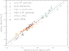 |
Fig. A.1. Star formation rate as a function of ISM pressure for the six galaxy samples. The lines correspond to an outlier-resistant linear bisector fit and its dispersion. The slope is 0.87 ± 0.02. |
The radially-averaged gas fraction converted to stars per free-fall time is ϵff = tff/tdep where tff is calculated at the scale of ldriv (Krumholz & McKee 2005), can be compared to the value of ϵff = 0.01 determined by Krumholz et al. (2012). For our main sequence samples (ordered by increasing z), we find ϵff = 0.004 ± 0.001, 0.010 ± 0.006, 0.018 ± 0.007 and for the starburst sequence, ϵff = 0.022 ± 0.007, 0.024 ± 0.031, 0.075 ± 0.041 as described in Sect. 2. It is clear that while ϵff increases with redshift in both samples, the starburst galaxies convert their gas more quickly into stars. Except for the high-z starbursts, these values are close to the Krumholz et al. (2012) prediction.
For self-gravitating clouds with a virial parameter of two (Bertoldi & McKee 1992), the turbulent crossing time tturb, cl equals 1.4 times the free-fall time tturb, cl:
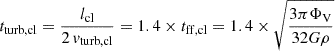 (A.2)
(A.2)
where lcl and vturb, cl are the size and the turbulent 1D velocity dispersion of a single gas cloud, respectively. Following Larson’s law (Larson 1981), we can simplify the expression of the turbulent crossing time:
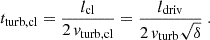 (A.3)
(A.3)
where δ is the scaling between the driving length scale and the size of the largest self-gravitating structures, such as δ = ldriv/lcl. The expression for the SFR then becomes
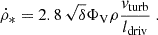 (A.4)
(A.4)
and  .
.
The SFR density is used to calculate the rate of energy injection by supernovae (SNe):
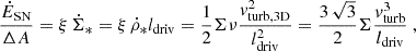 (A.5)
(A.5)
where ΔA is the unit surface element of the disk,  and
and  the star formation per unit area and unit volume, Σ the total gas surface density, ν the turbulent viscosity, vturb the turbulent velocity of the gas, and the CO disk thickness is assumed to be ldriv. The turbulent viscosity is
  . The energy injection rate is related to the turbulent velocity dispersion and the driving scale of turbulence. These quantities in turn provide estimates of the clumpiness of gas in the disk (i.e., the contrast between local and average density) and the rate at which viscosity moves matter inward. The derived expressions for ΦV and
  are
are
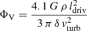 (A.6)
(A.6)
and
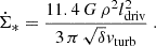 (A.7)
(A.7)
The model relies on several empirical calibrations: the relation between the stellar velocity dispersion and the stellar disk scale length, the relationship between the star-formation rate (SFR) and the energy injected into the ISM by SNe, and the characteristic time of H2 formation, which is related to the gas metallicity and the gas density. The fraction between the molecular and the total gas mass is governed by the turbulent crossing time  and the molecule formation timescale. In addition, photodissociation of molecules is taken into account.
The model is divided into a large-scale and a small-scale part. The former yields the surface density, turbulent velocity, disk height, and gas viscosity. The latter is relevant for self-gravitating gas clouds  . The non-self-gravitating and self-gravitating clouds obey different scaling relations, which are set by observations. For each gas density, the mass fraction of clouds of this density is characterized by a log-normal probability distribution function and the Mach number (Padoan et al. 1997). The temperatures of the gas clouds are calculated via the equilibrium between turbulent mechanical and cosmic ray heating and gas cooling via CO and H2 line emission. The abundances of the different molecules are determined using the time-dependent gas-grain code Nautilus (Hersant et al. 2009). The dust temperatures are calculated via the equilibrium between heating by the interstellar UV and optical radiation field and cooling via IR emission.
Appendix B: The model radio continuum emission
In this section, we briefly describe the parts of the model where nothing has changed with respect to what was done in V22. Under the assumption described in Sect. 4.3, the synchrotron emissivity is given by the density per unit energy interval of the primary CR electrons  and
and
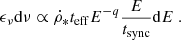 (B.1)
(B.1)
According to V22, the effective lifetime of synchrotron-emitting CR electrons teff is given by
 (B.2)
(B.2)
For the characteristic timescales, we follow the prescriptions of Lacki et al. (2010). The diffusion timescale based on observations of beryllium isotope ratios at the solar circle (Connell 1998, Webber et al. 2003) is
 (B.3)
(B.3)
where the mean energy E is calculated via the mean synchrotron frequency. The characteristic time for bremsstrahlung is
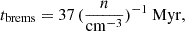 (B.4)
(B.4)
and that for inverse Compton energy losses is
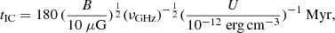 (B.5)
(B.5)
where U is the interstellar radiation field. The timescale of ionization-energy loss is
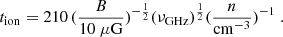 (B.6)
(B.6)
The magnetic field strength B is calculated under the assumption of energy equipartition between the turbulent kinetic energy of the gas and the magnetic field:
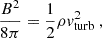 (B.7)
(B.7)
where ρ is the total midplane density of the gas and vturb its turbulent velocity dispersion.
Secondary CR electrons can be produced via collisions between the interstellar medium (ISM) and CR protons. The proton lifetime to pion losses (Mannheim & Schlickeiser 1994) is
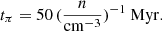 (B.8)
(B.8)
The effective lifetime of CR protons is given by
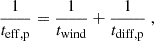 (B.9)
(B.9)
where the proton diffusion timescale is four times shorter than the CR electron diffusion timescale (Appendix B3 of Werhahn et al. 2021a). The CR electron secondary fraction is given by
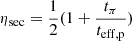 (B.10)
(Werhahn et al. 2021a). In models that include CR electron secondaries, the CR electron density is multiplied by (1 + ηsec).
With ν = CBE2, the synchrotron emissivity of Eq. B.1 becomes
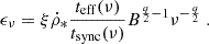 (B.11)
The constant is C = e/(2πme2c2). With the CR electron density n0 and
 (B.12)
the classical expression ϵν ∝ n0B(q + 1)/2ν(1 − q)/2 is recovered. The factor ξ was chosen such that the radio–IR correlations measured by Yun et al. (2001) and Molnar et al. (2021) are reproduced within 2σ (Fig. 15). As in Sect. 4.2 we assumed q = 2.3. The gas density ρ, turbulent gas velocity dispersion vturb, and interstellar radiation field U are directly taken from the analytical model of Sect. 4.1.
Following Tsang (2007) and Beck & Krause (2005), the synchrotron emissivity is given by
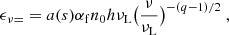 (B.13)
with a(s) = 3q/2/(4π(q + 1)) Γ((3s + 19)/12) Γ((3s − 1)/12), αf is the fine structure constant, h the Planck constant, and νL the Larmor frequency.
The synchrotron luminosity was calculated via
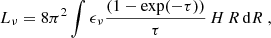 (B.14)
where τ = τff + τsync is the optical depth caused by free-free and synchrotron self-absorption.
For the free-free absorption we used
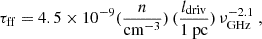 (B.15)
where the height of the star-forming disk is assumed to be of the order of the turbulent driving length scale. For the optical depth of synchrotron self-absorption, we used the formalism described by Tsang (2007).
Optically thin thermal emission was added according to the recipe of Murphy et al. (2012)
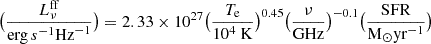 (B.16)
with an electron temperature of Te = 8000 K.
For the galaxies at high redshifts, the inverse Compton (IC) losses from the cosmic microwave background (CMB) are taken into account via the IC equivalent magnetic field:
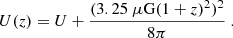 (B.17)
All Tables
All Figures
|
Fig. 1. PHIBSS2 stellar surface density profiles and rotation curves. Left panels: Decomposition of the stellar surface density profiles (bulge with a Sérsic index n = 4 and a disk with n = 1). Middle panel: Rotation curve decomposition (bulge, disk, and dark matter). Right panels: HST i-band images (F19) with the galaxy delimited by an ellipse. |
| In the text | |
|
Fig. 2. PHIBSS2 galaxies (F19). Maximum rotation velocity as a function of the stellar mass. The dashed and dotted black lines show vrot ∝ M*β with β = 0.22 and 0.25, respectively. The dotted gray lines show a scatter of 0.15 dex (Di Teodoro et al. 2021). |
| In the text | |
|
Fig. 3. Cosmic rays in the solar neighborhood. Upper panel: Model CR particle density spectra. Middle panel: CR energy spectra. The solid black line shows the CR electron model (Pohl 1993), the solid red line shows the CR proton model (Pohl 1993), the solid blue line shows the GALPROP model fit to observations by Cummings et al. (2016), and triangles shows Voyager 1 data (Cummings et al. 2016) and AMS data (Aguilar et al. 2019). Lower panel: CR injection spectra. |
| In the text | |
|
Fig. 4. Infrared spectral energy distributions. Red pluses and solid line: model SED. Red dashed line: modified Planck fit for temperature determination. Black crosses: VizieR photometry. The errors bars are shown, if present in the VizieR tables, but often barely visible. Upper panel: z ∼ 0.5 LIRGs. Lower panel: local LIRGs. |
| In the text | |
|
Fig. 5. Model CO luminosities as a function of the observed CO luminosities. The model CO transition corresponds to the observed transition. The lines correspond to the one-to-one relation with a scatter of a factor of two. |
| In the text | |
|
Fig. 6. Distribution of galaxy metallicities. The solid black line shows the local SF galaxies. The dotted blue line shows local starbursts. The dashed green line shows high-z starbursts. The dash-dotted red line shows high-z SF galaxies. The yellow line shows local LIRGs. The orange line shows z ∼ 0.5 LIRGs. The solar metallicity is assumed to be 12+log(O/H) = 8.7. |
| In the text | |
|
Fig. 7. Model total IR luminosity as a function of the observed TIR luminosity of the galaxies. The lines correspond to an outlier-resistant linear bisector fit and its dispersion. |
| In the text | |
|
Fig. 8. Model distribution of dust temperatures. Black solid line: local SF galaxies. Blue dotted line: local starbursts. Green dashed line: high-z starbursts. Red dash-dotted line: high-z SF galaxies. Yellow: local LIRGs. Orange: z ∼ 0.5 LIRGs. |
| In the text | |
|
Fig. 9. Model HCN(1–0) luminosities as a function of the model TIR luminosities. The upper solid line corresponds to L′HCN/LTIR = 980 (Jiménez-Donaire et al. 2019), and the dashed lines are offset by a factor of 0.5 and 2. The lower solid line corresponds to a 2.3 lower L′HCN/LTIR as found for luminous IR galaxies by García-Burillo et al. (2012). |
| In the text | |
|
Fig. 10. Model HCN(1–0) (upper panel) and HCO+(1-0) (lower panel) luminosity as a function of the observed HCN(1–0)/HCO+(1-0) luminosity (Graciá-Carpio et al. 2008). The solid line corresponds to the one-to-one relation, and the dotted lines show a dispersion of 0.3 dex. The dashed lines correspond to a robust bisector fit. |
| In the text | |
|
Fig. 11. Mean model CO SLEDs of our galaxy samples. The dotted line corresponds to a constant brightness temperature. The high-z SF galaxy sample was divided into a z ∼ 1.5 (solid red) and a z > 2 (dashed red) subsample. IRAS 08339+6517 is shown by the dashed black line. |
| In the text | |
|
Fig. 12. CO SLEDs of local starburst galaxies (ULIRGs). Upper panel: the black boxes linked by black lines represent the observed mean CO SLEDs of ULIRGs with total IR luminosities between 3 × 10¹¹ and 1012 L⊙ and higher than 1012 L⊙, respectively (from Kamenetzky et al. 2016). Lower panels: model (pluses) and observed CO SLEDs (Rosenberg et al. 2015; triangles). |
| In the text | |
|
Fig. 13. CO(1–0) conversion factors for our galaxy samples in units of M⊙(K km s−1pc2)−1. |
| In the text | |
|
Fig. 14. HCN conversion factors in units of M⊙(K km s−1pc2)−1. Upper panel: HCN(1–0)–dense gas conversion factors; lower panel: HCN(1-0)–MH2 conversion factors for our galaxy samples. |
| In the text | |
|
Fig. 15. IR-radio correlations. Upper left: 70 μm – 1.4 GHz correlation. Upper right: 100 μm – 1.4 GHz correlation. Lower left: 160 μm – 1.4 GHz correlation. Lower right: TIR – 1.4 GHz correlation. The colored and black symbols show model galaxies. For clarity, the z ∼ 0.5 LIRGs are shown as yellow diamonds in the lower right panel. The solid and dotted black lines mark the model linear regression. The gray dots show the observations. |
| In the text | |
|
Fig. 16. TIR–1.4 GHz correlations. The symbols show the model galaxies. Black solid and dotted lines show the model linear regression. Upper panel: Gray solid and dashed lines show the observed linear regression (Beck 2015). Lower panel: Orange error bars show data from Bell (2003). Gray solid and dashed lines mark the observed linear regression (Bell 2003). |
| In the text | |
|
Fig. 17. Upper panel: SFR–1.4 GHz correlation. Lower panel: SFR–150 MHz correlation. The colored lines show observed correlations. The pluses mark the model galaxies. The dashed black lines in both panels correspond to outlier-resistant linear bisector fits. |
| In the text | |
|
Fig. 18. CO SLEDs of the local starburst galaxies with 1.5 to two times higher Q values compared to Fig. 12. Black triangles: Rosenberg et al. (2015). Green lines: models. |
| In the text | |
|
Fig. 19. Star formation rate per unit area as a function of the molecular gas surface density. The dotted lines show linear and square fits to guide the eye. The dashed lines show robust fits to the different galaxy samples. |
| In the text | |
|
Fig. 20. Molecular gas depletion time. Upper panel: as a function of the sSFR for the model galaxies. Middle panel: as a function of the sSFR for the observations from Saintonge et al. (2017). Lower panel: as a function of redshift for the model galaxies. The lines correspond to an outlier-resistant linear bisector fit and its dispersion. |
| In the text | |
|
Fig. 21. Star formation efficiency. Upper panel: Star formation efficiency with respect to the molecular gas as a function of the angular velocity Ω. The lines correspond to an outlier-resistant linear bisector fit and its dispersion. Lower panel: Star formation efficiency with respect to the molecular gas as a function of the turbulent velocity dispersion. The fit only applies to the SF galaxies. |
| In the text | |
|
Fig. 22. Model turbulent velocity as a function of the SFR (upper panel), the SFR per unit area (middle panel), and the gas fraction (lower panel). The filled circles and boxes correspond to observed values (Downes & Solomon 1998; Cresci et al. 2009; Tacconi et al. 2013; Girard et al. 2021; Nestor Shachar et al. 2023). The lines correspond to an outlier-resistant linear bisector fit and its dispersion. |
| In the text | |
|
Fig. 23. Upper panel: Inverse of the overdensity of selfgravitating clouds as a function of the turbulent velocity dispersion. The solid line corresponds to an outlier-resistant linear bisector fit, and the dashed line shows ΦV = vturb/(1 km s−1)/7000. Lower panel: Star formation efficiency with respect to the molecular gas as function of (vturb × Ω). The solid and dotted lines correspond to an outlier-resistant linear bisector fit and its dispersion. The dashed line corresponds to SFE = 10−3 vturbΩ. |
| In the text | |
|
Fig. 24. Fraction tvisc/t* as a function of the stellar mass of the model galaxies. Upper panel: SF galaxies. The tvisc/t* fractions of the star-forming galaxies should thus be taken as lower limits with an uncertainty of a factor of two towards higher values. The dashed lines are observed trends with stellar mass. Lower panel: Starburst galaxies. |
| In the text | |
|
Fig. 25. Models with k = 9 instead of k = 3. Upper panel: Model CO flux of the galaxies of the different samples as a function of the observed CO flux. Lower panel: Model HCN(1–0) flux as a function of the observed HCN(1–0) flux for the local starburst galaxies. |
| In the text | |
|
Fig. 26. Models without the dependence of ζH on the gas column density. Upper panel: Model CO flux of the galaxies of the different samples as a function of the observed CO flux. Lower panel: Model HCN(1–0) flux as a function of the observed HCN(1–0) flux for the local starburst galaxies. |
| In the text | |
|
Fig. A.1. Star formation rate as a function of ISM pressure for the six galaxy samples. The lines correspond to an outlier-resistant linear bisector fit and its dispersion. The slope is 0.87 ± 0.02. |
| In the text | |
Current usage metrics show cumulative count of Article Views (full-text article views including HTML views, PDF and ePub downloads, according to the available data) and Abstracts Views on Vision4Press platform.
Data correspond to usage on the plateform after 2015. The current usage metrics is available 48-96 hours after online publication and is updated daily on week days.
Initial download of the metrics may take a while.