| Issue |
A&A
Volume 661, May 2022
|
|
|---|---|---|
| Article Number | A119 | |
| Number of page(s) | 28 | |
| Section | Stellar structure and evolution | |
| DOI | https://doi.org/10.1051/0004-6361/202141613 | |
| Published online | 13 May 2022 | |
Angular momentum transport in a contracting stellar radiative zone embedded in a large-scale magnetic field
Institut de Recherche en Astrophysique et Planétologie (IRAP), Université de Toulouse, 14 avenue Edouard Belin, 31400 Toulouse, France
e-mail: bgouhier@irap.omp.eu; ljouve@irap.omp.eu; flignieres@irap.omp.eu
Received:
22
June
2021
Accepted:
7
January
2022
Context. Some contracting or expanding stars are thought to host a large-scale magnetic field in their radiative interior. By interacting with the contraction-induced flows, such fields may significantly alter the rotational history of the star. They thus constitute a promising way to address the problem of angular momentum transport during the rapid phases of stellar evolution.
Aims. In this work, we aim to study the interplay between flows and magnetic fields in a contracting radiative zone.
Methods. We performed axisymmetric Boussinesq and anelastic numerical simulations in which a portion of the radiative zone was modelled by a rotating spherical layer, stably stratified and embedded in a large-scale (either dipolar or quadrupolar) magnetic field. This layer is subject to a mass-conserving radial velocity field mimicking contraction. The quasi-steady flows were studied in strongly or weakly stably stratified regimes relevant for pre-main sequence stars and for the cores of subgiant and red giant stars. The parametric study consists in varying the amplitude of the contraction velocity and of the initial magnetic field. The other parameters were fixed with the guidance of a previous study.
Results. After an unsteady phase during which the toroidal field grew linearly and then back-reacted on the flow, a quasi-steady configuration was reached, characterised by the presence of two magnetically decoupled regions. In one of them, magnetic tension imposes solid-body rotation. In the other, called the dead zone, the main force balance in the angular momentum equation does not involve the Lorentz force and a differential rotation exists. In the strongly stably stratified regime, when the initial magnetic field is quadrupolar, a magnetorotational instability is found to develop in the dead zones. The large-scale structure is eventually destroyed and the differential rotation is able to build up in the whole radiative zone. In the weakly stably stratified regime, the instability is not observed in our simulations, but we argue that it may be present in stars.
Conclusions. We propose a scenario that may account for the post-main sequence evolution of solar-like stars, in which quasi-solid rotation can be maintained by a large-scale magnetic field during a contraction timescale. Then, an axisymmetric instability would destroy this large-scale structure and this enables the differential rotation to set in. Such a contraction-driven instability could also be at the origin of the observed dichotomy between strongly and weakly magnetic intermediate-mass stars.
Key words: instabilities / magnetohydrodynamics (MHD) / methods: numerical / stars: magnetic field / stars: rotation / stars: interiors
© B. Gouhier et al. 2022
 Open Access article, published by EDP Sciences, under the terms of the Creative Commons Attribution License (https://creativecommons.org/licenses/by/4.0), which permits unrestricted use, distribution, and reproduction in any medium, provided the original work is properly cited.
1. Introduction
Rotation is ubiquitous at every stage of stellar evolution. Yet, it is still often considered as a second order effect in stellar evolution models. A full description necessarily entails a thorough study of differential rotation and meridional circulation induced by rotation, how they interact with other physical processes (e.g. magnetic field or internal gravity waves), and the ensuing potential instabilities. In his seminal work, Zahn (1992) proposed a model for the transport of chemical elements and angular momentum (AM) (without a magnetic field and internal gravity waves) that was later implemented in state-of-the-art stellar evolution codes. One of the strong assumptions is that the differential rotation in radiative zones is close to shellular (i.e. constant on an isobar) because of the anisotropic turbulence induced by shear instabilities in stably stratified conditions. This formalism has been successful at explaining a large number of stellar observations (see Maeder 2008 for a review). However, a growing body of evidence shows that additional AM transport mechanisms are still needed. This is particularly true for contracting stars. During the pre-main sequence (PMS) or post-MS evolution, a spin-up of stellar cores is naturally produced. However, observations of surface rotation of stars in young clusters (Gallet & Bouvier 2013) as well as asteroseismic studies of red giant stars (Eggenberger et al. 2012; Ceillier et al. 2013; Marques et al. 2013) tend to show that rotation rates are in fact strongly overestimated in models. In order to improve this formalism, the first thing to ask is what kind of flows are really expected in those contracting stars.
In a previous work (Gouhier et al. 2021), we investigated the differential rotation and meridional circulation produced in a modelled contracting stellar radiative zone. This axisymmetric study included the effects of stable stratification and was conducted both under the Boussinesq and the anelastic approximations, but the effects of a magnetic field were ignored. We showed that a radial differential rotation should be expected only in strongly stably stratified radiative zones such as the degenerate cores of subgiants. Indeed, any meridional circulation is inhibited by the strong buoyancy force, and the characteristic amplitude of the differential rotation in the linear regime is found to be proportional to the ratio of the viscous to contraction timescales ΔΩ/Ω0 ∝ τν/τc. In conditions relevant for the outside of the degenerate cores of subgiants and for PMS stars though, thermal diffusion weakens the stable stratification and allows a meridional circulation to exist, with a typical amplitude of the order of the contraction speed. The differential rotation profile then exhibits both a dependence in latitude and radius and its characteristic amplitude in the linear regime is found to be ΔΩ/Ω0 ∝ τED/τc, where τED is the Eddington–Sweet timescale associated with the AM transport by the meridional flow. Both estimates, assuming a contraction timescale comparable to the Kelvin-Helmholtz timescale, tend to indicate that the amplitude of the differential rotation can be quite strong and that another process of AM transport should be invoked to reproduce the rotation rates of pre-MS and post-MS stars.
The presence of a large-scale magnetic field in such contracting radiative zones can drastically modify this picture. It is commonly agreed that radiative zones can host such fields (see Braithwaite & Spruit 2017 for a review). Magnetic fields with surface intensities of a few hundred Gauss have indeed been detected in a fraction of intermediate-mass PMS stars (Alecian et al. 2013). These stars are most probably the progenitors of the MS chemically peculiar Ap/Bp stars that host large-scale mostly dipolar fields with intensities ranging from 300 G to 30 kG (Donati & Landstreet 2009). Meanwhile, a distinct population of MS intermediate-mass stars, including the A-type star Vega and the Am-type stars Sirius, β Ursae Majoris and θ Leonis, exhibits much weaker (∼1 G) multi-polar magnetic fields (Lignières et al. 2009; Petit et al. 2010, 2011; Blazère et al. 2016). This magnetic dichotomy could be explained if, during the PMS, contraction forces a differential rotation that destroys pre-existing large-scale weak magnetic fields through magnetohydrodynamic (MHD) instabilities (Aurière et al. 2007; Lignières et al. 2014; Jouve et al. 2015, 2020).
Unlike PMS stars, the radiative zone of post-MS stars is overlaid by a large convective envelope preventing any direct measurement of a magnetic field in the convectively stable regions. Recently, asteroseismology revealed a class of red giants exhibiting dipolar oscillation modes with a very weak visibility (Mosser et al. 2012). This phenomenon has been attributed to the presence of an internal magnetic field modifying the angular structure of the dipole waves, thus leading to their trapping in the radiative core (Fuller et al. 2015). This so-called greenhouse effect, supported by other authors (Stello et al. 2016a,b; Cantiello et al. 2016) is, however, seriously questioned because these modes preserve their mixed character at odds with Fuller’s scenario (Mosser et al. 2017). In parallel, the possibility to detect magnetic fields through their effect on the oscillation frequencies is under investigation (see e.g. Bugnet et al. 2021). Awaiting observational evidence, theoretical work strongly supports the presence of magnetic fields in stars that possess a convective core (MS stars with M ≳ 1.2 M⊙). The numerical simulations of core-dynamos of MS A- and B-type stars (Brun et al. 2005; Augustson et al. 2016) indicate that magnetic fields with intensities ranging from 0.1 − 1.0 MegaGauss can indeed be generated. Such a magnetic field could then relax into a large-scale stable configuration in the radiative interior of the post-MS stars where it would be buried for the rest of its evolution (Braithwaite & Spruit 2004).
Large-scale magnetic fields are able to impose a quasi-solid rotation on very short timescales, even for very weak intensities (Ferraro 1937; Mestel & Weiss 1987). Besides, enforcing a quasi-solid rotation during ∼1 Gyr after the end of the MS enabled Spada et al. (2016) to reproduce the rotation rates of subgiants, as measured by asteroseismology (Deheuvels et al. 2014). This result was also obtained by Eggenberger et al. (2019) and an observational support was then provided by Deheuvels et al. (2020) who measured a near solid rotation in two young subgiants. Interestingly, the efficiency of the AM transport then seems to decrease up to the tip of the red giant branch (RGB) before increasing again (Spada et al. 2016; Eggenberger et al. 2019; Deheuvels et al. 2020). Those works suggest a scenario broken down into several key phases. First, a quasi-solid rotation is maintained for some time through an efficient AM transport mechanism (possibly magnetic tension imposed by a large-scale field). Then, this mechanism would become inefficient and differential rotation would build up again before another AM transport mechanism, such as turbulent transport induced by MHD instabilities (Spruit 2002; Rüdiger et al. 2015; Fuller et al. 2019; Jouve et al. 2020) takes over.
In this work, we intend to study the flows induced by a contracting radiative zone in the presence of a large-scale magnetic field, through axisymmetric MHD simulations. In particular, we focus on the structure of the steady-states differential rotation and on the ability of the magnetic field to transport AM. The paper is organised as follows: in Sect. 2 we present the mathematical model, then in Sect. 3, the different timescales involved in our problem. The initial and boundary conditions as well as the numerical method are described in Sects. 4 and 5 respectively. In Sect. 6 we provide the reader with the relevant timescales in the stellar context and the consequences for our numerical study. The results of the simulations in the viscous and Eddington–Sweet regimes are finally given in Sect. 7, and are then summarised in Sect. 8 where the astrophysical implications are also discussed.
2. Mathematical formulation
In our previous work (Gouhier et al. 2021), we investigated the differential rotation and meridional flows produced in a contracting stellar radiative zone. In this follow-up work, we add the effect of an initial large-scale magnetic field. To do so, we numerically solve the Boussinesq or anelastic magnetohydrodynamical (MHD) equations in a spherical shell filled with a stably-stratified fluid subject to a radial contraction and embedded in a magnetic field. In this section we present the governing equations that we numerically solve in the two aforementioned approximations.
In this study, the fluid contraction is modelled using a mass-conserving contraction velocity field defined by
where r is the radius and  the background density, r0 and ρ0 their respective values at the outer sphere and V0 is the amplitude of the contraction velocity at the outer sphere. Using the Lantz-Braginsky-Roberts (LBR) approximation (Lantz 1992; Braginsky & Roberts 1995), assuming a uniform kinematic viscosity ν, thermal diffusion κ, magnetic diffusion η, and neglecting the centrifugal effects and local sources of heat, the dimensionless axisymmetric anelastic equations of a magnetised fluid (Jones et al. 2011) undergoing contraction read
![$$ \begin{aligned} \begin{array}{lll} \boldsymbol{\nabla } \cdot \left[\tilde{\overline{\rho }} \left( \boldsymbol{\tilde{U}} + \boldsymbol{\tilde{V}}_{f} \right) \right]= 0 \quad \mathrm{and} \quad \boldsymbol{\nabla } \cdot \boldsymbol{\tilde{B}} = 0 , \end{array} \end{aligned} $$](/articles/aa/full_html/2022/05/aa41613-21/aa41613-21-eq3.gif)
![$$ \begin{aligned}&R_o \left[\displaystyle \frac{\partial \boldsymbol{\tilde{U}}}{\partial t} + \left( \left( \boldsymbol{\tilde{U}} + \boldsymbol{\tilde{V}}_{f} \right) \cdot \boldsymbol{\nabla } \right) \left( \boldsymbol{\tilde{U}} + \boldsymbol{\tilde{V}}_{f} \right) \right]+ 2 \boldsymbol{e}_z \times \left( \boldsymbol{\tilde{U}} + \boldsymbol{\tilde{V}}_{f} \right)\nonumber \\&= - \boldsymbol{\nabla } \!\left( \displaystyle \frac{\tilde{\Pi }^{\prime }}{\tilde{\overline{\rho }}} \right) + \displaystyle \frac{\tilde{S}^{\prime }}{\tilde{r}^2} \boldsymbol{e}_r +\displaystyle \! \frac{E}{\tilde{\overline{\rho }}} \ \boldsymbol{\nabla } \cdot \boldsymbol{\boldsymbol{\tilde{\sigma }}} + \! \left( \displaystyle \!\frac{L_u E}{P_m} \right)^2 \displaystyle \frac{R_o^{-1}}{\tilde{\overline{\rho }}} \left[\left(\boldsymbol{\nabla } \times \boldsymbol{\tilde{B}} \right) \times \boldsymbol{\tilde{B}} \right], \end{aligned} $$](/articles/aa/full_html/2022/05/aa41613-21/aa41613-21-eq4.gif)
![$$ \begin{aligned} \displaystyle \frac{\partial \boldsymbol{\tilde{B}}}{\partial t} = \boldsymbol{\nabla } \times \left[\left( \boldsymbol{\tilde{U}} + \boldsymbol{\tilde{V}}_{f} \right) \times \boldsymbol{\tilde{B}} \right]+ \displaystyle \frac{1}{R_m} \boldsymbol{\nabla }^2 \boldsymbol{\tilde{B}} , \end{aligned} $$](/articles/aa/full_html/2022/05/aa41613-21/aa41613-21-eq5.gif)
![$$ \begin{aligned}&\tilde{\overline{\rho }} \tilde{\overline{T}} \left[P_r R_o \left( \displaystyle \frac{\partial \tilde{S}^{\prime }}{\partial t} \right. + \left( \left( \boldsymbol{\tilde{U}} + \boldsymbol{\tilde{V}}_{f} \right) \cdot \boldsymbol{\nabla } \right) \tilde{S}^{\prime } \right) + P_r \left( \displaystyle \frac{N_0}{\Omega _0} \right)^2 \left( \tilde{U}_r + \tilde{V}_{f} \right) \left. \displaystyle \frac{\mathrm{d} \tilde{\overline{S}}}{\mathrm{d} r} \right]\nonumber \\&\ = E \ \boldsymbol{\nabla } \cdot \! \left( \tilde{\overline{\rho }} \tilde{\overline{T}} \boldsymbol{\nabla } \tilde{S}^{\prime } \right)\! + D_i Pe_c E^2 \left[\tilde{\mathcal{Q} }{_{\nu }} + P_m^{-1} \!\left(\displaystyle \frac{L_u E}{P_m R_o} \right)^2\! \left( \boldsymbol{\nabla } \times \boldsymbol{\tilde{B}} \right)^2 \right], \end{aligned} $$](/articles/aa/full_html/2022/05/aa41613-21/aa41613-21-eq6.gif)
where the diffusion of entropy is introduced in the energy equation instead of the diffusion of temperature (Braginsky & Roberts 1995; Clune et al. 1999). The non-dimensional form (identified by the tilde variables) of these equations is obtained using the radius of the outer sphere r0 as the reference lengthscale, the value of the contraction velocity field at the outer sphere V0 as a characteristic velocity, and τc = r0/V0 as the reference timescale of the contraction. The frame rotates at Ω0, the rotation rate of the outer sphere and all the thermodynamics variables are expanded as a background value plus fluctuations, respectively denoted with an overbar and a prime. The background density and temperature field are non-dimensionalised respectively by the outer sphere density ρ0 and temperature T0, while the background gradients of temperature and entropy fields are adimensionalised using the temperature and entropy difference  and
and  between the two spheres. The pressure fluctuations are non-dimensionalised by ρ0r0Ω0V0 and the entropy fluctuations by CpΩ0V0/g0, where Cp is the heat capacity and g0 the gravity at the outer sphere. Finally, we use the value of the surface poloidal field at the poles B0 as the reference scale for the magnetic field.
In Eqs. (2)–(5), U is the velocity field,  is the dimensionless stress tensor,
  is the dimensionless viscous heating and the gravity profile is ∝r−2. The reference state is non-adiabatic and a uniform positive entropy gradient is used to produce a stable stratification. It is related to the Brunt-Väisälä frequency defined by:
and which controls the amplitude of this stable stratification. The magnitude of the deviation to the isentropic state is controlled by the parameter  , chosen sufficiently small to ensure the validity of the anelastic approximation. With the dissipation number Di = g0r0/T0Cp, it sets the background temperature and density profiles (see Gouhier et al. 2021).
These anelastic equations involve six independent dimensionless numbers, a Rossby number based on the amplitude of the contraction velocity Ro = V0/Ω0r0, the Ekman number  , the Prandtl number Pr = ν/κ, the ratio between the reference Brunt-Väisälä frequency and the rotation rate of the outer sphere N0/Ω0, the magnetic Prandtl number Pm = ν/η, and the Lundquist number
  where μ0 is the vacuum permeability. From these dimensionless numbers, three additional parameters can then be defined: a contraction Reynolds number Rec = Ro/E, a Péclet number Pec = PrRec, and a magnetic Reynolds number Rm = PmRec.
When the compressibility effects are neglected, except in the buoyancy term of the momentum equation, the Boussinesq approximation is recovered. In that case, using Ω0V0T0/g0 as the scale of the temperature deviations Θ′, the dimensionless governing equations read
![$$ \begin{aligned}&R_o \left[\displaystyle \frac{\partial \boldsymbol{\tilde{U}}}{\partial t} + \left( \left( \boldsymbol{\tilde{U}} + \boldsymbol{\tilde{V}}_{f} \right) \cdot \boldsymbol{\nabla } \right) \left( \boldsymbol{\tilde{U}} + \boldsymbol{\tilde{V}}_{f} \right)\right]+ 2 \boldsymbol{e}_z \times \left( \boldsymbol{\tilde{U}} + \boldsymbol{\tilde{V}}_{f} \right) \nonumber \\&\ = - \boldsymbol{\nabla } \tilde{\Pi }^{\prime } + \tilde{\Theta }^{\prime } \boldsymbol{\tilde{r}} + E \ \boldsymbol{\nabla }^2\left( \boldsymbol{\tilde{U}} + \boldsymbol{\tilde{V}}_{f} \right) + \left( \displaystyle \frac{L_u E}{P_m} \right)^2 R_o^{-1} \left[\left(\boldsymbol{\nabla } \times \boldsymbol{\tilde{B}} \right) \times \boldsymbol{\tilde{B}} \right], \end{aligned} $$](/articles/aa/full_html/2022/05/aa41613-21/aa41613-21-eq16.gif)
![$$ \begin{aligned} \displaystyle \frac{\partial \boldsymbol{\tilde{B}}}{\partial t} = \boldsymbol{\nabla } \times \left[\left( \boldsymbol{\tilde{U}} + \boldsymbol{\tilde{V}}_{f} \right) \times \boldsymbol{\tilde{B}} \right]+ \displaystyle \frac{1}{R_m} \boldsymbol{\nabla }^2 \boldsymbol{\tilde{B}} , \end{aligned} $$](/articles/aa/full_html/2022/05/aa41613-21/aa41613-21-eq17.gif)
![$$ \begin{aligned}&P_r R_o \left[\displaystyle \frac{\partial \tilde{\Theta }^{\prime }}{\partial t} + \left( \left( \boldsymbol{\tilde{U}} + \boldsymbol{\tilde{V}}_{f} \right) \cdot \boldsymbol{\nabla } \right) \tilde{\Theta }^{\prime } \right]+ P_r \left( \displaystyle \frac{N_0}{\Omega _0} \right)^2 \left( \tilde{U}_r + \tilde{V}_{f} \right) \displaystyle \frac{\mathrm{d} \tilde{\overline{T}}}{\mathrm{d} r} \nonumber \\&\quad = E \boldsymbol{\nabla }^2 \tilde{\Theta }^{\prime } , \end{aligned} $$](/articles/aa/full_html/2022/05/aa41613-21/aa41613-21-eq18.gif)
where the gravity profile is now ∝r, the reference Brunt-Väisälä frequency is defined using the correspondence  in Eq. (6), and the contraction velocity field Eq. (1) is simplified using
  .
.
To conclude this section, we note that when the anelastic approximation is used the parameter space is defined by eight dimensionless numbers: ϵs, Di, Rec, E, Pr, Pm, Lu and  . Instead, only the last six are necessary in the Boussinesq approximation. In this study, only Rec, Lu and the product Pr(N0/Ω0)2 will be varied.
3. Timescales of physical processes
In this section, we describe the various timescales involved in the transport of AM in our problem. We start by briefly recalling the relevant hydrodynamical timescales (see Gouhier et al. 2021), then we introduce two timescales associated with the presence of a magnetic field.
In this work, the dimensional form of the AM equation under the Boussinesq approximation reads
where D2 is the azimuthal component of the vector Laplacian operator, Us = cos θUθ + sin θUr is the component of the velocity field, perpendicular to the rotation axis, and NL denotes the non-linear advection term. By balancing the partial time derivative with the contraction term in Eq. (11), we recover the contraction timescale used to non-dimensionalise the governing equations in Sect. 2

as well as its linear form
when ΔΩ/Ω0 ≪ 1. In the anelastic approximation, the contraction term in Eq. (11) is multiplied by  and the resulting timescale is then weighted by the background density profile
where  denotes the linear version. The AM transport by contraction can be balanced either by the viscous processes on a viscous timescale
  , or by a meridional circulation of Eddington–Sweet type, in which case it redistributes the AM on the following timescale
Ekman layers tend to develop at the spherical boundaries to accommodate the interior flow to the boundary conditions. In unstratified flows, they drive a global circulation. In stars, the stable stratification efficiently opposes this global flow although it can still exist in numerical simulations because the Ekman numbers can not reach stellar values. It then transports the AM on a spin-up timescale defined by

The relative importance of these AM redistribution processes is given by the ratio of the above timescales, namely:
Two main dimensionless numbers thus appear, the Ekman number E and the Pr(N0/Ω0)2 parameter. As first noticed by Garaud (2002), the latter is of prime interest since it controls the flow dynamics. Thus, at fixed Pr and N0, the author shows that depending on the rotation rate value this parameters defines two rotation regimes (slow or fast). More in line with our work, Garaud & Brummell (2008), Garaud & Garaud (2008), Garaud & Acevedo-Arreguin (2009), Wood & Brummell (2012, 2018), Acevedo-Arreguin et al. (2013) have shown that it also controls the efficiency of the burrowing of the meridional circulation in radiative layers adjacent to convective regions. In particular, when Pr(N0/Ω0)2 ≫ 1, this circulation is suppressed by the stable stratification, a situation similar to the one that we encountered in the viscous regime described in Gouhier et al. (2021). In our case, E and Pr(N0/Ω0)2 allow us to distinguish three regimes of interest:
As discussed in Gouhier et al. (2021), the two last regimes, namely the Eddington–Sweet regime τE ≪ τED ≪ τν and the viscous regime τE ≪ τν ≪ τED, are the most relevant for stars. We thus focus on them for the magnetic study.
The magnetic field introduces two new timescales: the magnetic diffusion timescale

and the Alfvén timescale
When the density contrast is taken into account (anelastic approximation), a new Alfvén timescale can be defined as
4. Initial and boundary conditions
Initially, we impose a dipolar or a quadrupolar poloidal magnetic field. In both cases, the radial distribution of the magnetic field is such that the azimuthal current density does not depend on r, (∂jϕ/∂r = 0), to avoid possible numerical instabilities resulting from strong current sheets at the boundaries. For the dipole topology (left panel in Fig. 1), the initial field reads
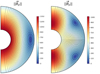 |
Fig. 1. Meridional cuts of the norm of the initial magnetic field (colour) for the dipole Eq. (22) (left), and the quadrupole Eq. (23) (right). The black lines show the poloidal field lines. |
For the quadrupole topology (right panel in Fig. 1), it takes the following form
Figure 1 shows that some field lines connect to the inner and outer boundaries while others are only connected to the outer boundary, or even loop-back on themselves inside the domain. In both configurations, the norm of the magnetic field at the poles and at the outer sphere is B0.
Insulated boundary conditions are imposed at the inner and outer spheres. For our axisymmetric setup, these conditions translate into

where Φ is a potential field.
The rotation rate is chosen to be initially uniform Ω(r, θ, t = 0) = Ω0 in the Boussinesq approximation. In the anelastic case, the initial profile is
where σ controls the amplitude of the differential rotation.
For all simulations, we impose stress-free conditions at the inner sphere for the latitudinal and azimuthal components of the velocity field, and impermeability condition for the radial component of the velocity field:
At the outer sphere, we impose an impermeability condition on the radial component of velocity field, and no-slip conditions on the latitudinal and azimuthal components of the velocity field:

the rotation rate of the outer sphere being thus fixed to Ω0. The boundary layers induced by these conditions in the absence of magnetic field were analysed in Gouhier et al. (2021).
Finally, in the Boussinesq approximation the temperature is prescribed at the inner and outer spheres, and the initial temperature field is the purely radial solution of the conduction equation. In the anelastic case, the entropy is also fixed at the boundaries. The initial stably stratified background density and temperature profiles are displayed in Gouhier et al. (2021).
5. Numerical method
The numerical study was carried out using the fully documented, publicly available code MagIC1 to solve the set of axisymmetric magneto-hydrodynamical equations in a spherical shell under the anelastic approximation (Gastine & Wicht 2012) (Eqs. (3)–(5)), or under the Boussinesq approximation (Wicht 2002) (Eqs. (8)–(10)). The solenoidal condition of Eqs. (2) and (7) is ensured by a poloidal–toroidal decomposition for the mass flux and the magnetic field. Then, the different fields are expanded on the basis of the spherical harmonics for the horizontal direction, and on the set of the Chebyshev polynomials for the radial direction. In particular, the Chebyshev discretisation guarantees a better resolution near the boundaries. The extent of the spherical shell can be reduced to a two-dimensional domain such as 𝒟 = {ri = 0.3 ≤ r ≤ r0 = 1.0;0 ≤ θ ≤ π}.
In the viscous regime, most of the simulations were performed with Nr × Nθ = 127 × 256, while for the most resolved cases Nr × Nθ = 193 × 512. In the Eddington–Sweet regime, a higher resolution was needed and for most of the simulations Nr × Nθ = 193 × 512, where Nr could be increased when the boundary layers needed to be carefully resolved.
6. Space of parameters
In this section, we estimate the relevant timescales in stars in order to constrain the regime of parameters of our numerical study.
6.1. The stellar context
The magnetic fields considered in this paper are large-scale fossil fields. They can be remnants of the proto-stellar phase, or the product of a core-dynamo buried in the radiative zone. At large scales, the ohmic diffusion timescale is around one Gyr (Braithwaite & Spruit 2017), that is longer than the MS lifetime of the intermediate mass-stars. Dynamic processes such as the Alfvén waves propagation occur over much shorter timescales, and we will always have

Typical magnetic Prandtl numbers in stellar plasmas are ∼5 × 10⁻³ − 10−2 (Rüdiger et al. 2016) so that τη ≪ τν. There is an exception though in the core of subgiants where the electrons are partially or fully degenerate. In that case, the Prandtl and magnetic Prandtl numbers increase because the thermal and magnetic diffusivities as well as the kinematic viscosity are dominated by the electron conduction (Garaud et al. 2015). The magnetic Prandtl number then ranges from 0.1 to 10 (Cantiello & Braithwaite 2011; Garaud et al. 2015; Rüdiger et al. 2015) and consequently, τη ≤ τν or τν ≤ τη.
In Gouhier et al. (2021), we already found that contracting stars (PMS or subgiant stars) always lie in the regime

In addition, we showed that the Eddington–Sweet regime is relevant for PMS stars and outside the degenerate core of subgiants. We thus have Pr(N0/Ω0)2 ≪ Pm ≪ 1, or τED ≪ τη ≪ τν, in these cases. By contrast, the degenerate cores of subgiants experience a viscous regime with higher Pm, such that 1 ∼ Pm ≪ Pr(N0/Ω0)2, that is τν ∼ τη ≪ τED.
We can now wonder how the Alfvén time compares to the contraction time in stars. We lack precise information about the magnetic field intensities within stars, but we can get some insight from the spectropolarimetric data of Herbig stars, or from the asteroseismology of red giant stars combined to numerical simulations. On the one hand, high-resolution spectropolarimetric surveys show that a small fraction of HAeBes hosts large-scale dipolar fields stronger than a hundred Gauss (Wade et al. 2005; Alecian et al. 2013). For a typical Herbig star of 3 M⊙ and 3 R⊙ hosting a magnetic field of 300 G, the Alfvén poloidal timescale, computed using the mean density of the star, would be of the order of a few tens of years. For these PMS stars, the mass is between 2 M⊙ and 5 M⊙ and the Kelvin-Helmholtz timescale τKH typically ranges from 23 to 1.2 Myr (Maeder 2008). Then, assuming τc ≈ τKH, implies that τAp ≪ τc.
On the other hand, the recent discovery of depressed dipole oscillation modes in red giants (Mosser et al. 2012) has been assigned to a greenhouse effect resulting from a strong magnetic field ∼1 MG trapping the gravity waves in the radiative core (Fuller et al. 2015). Although this scenario is controversial (see e.g. Mosser et al. 2017), the three-dimensional MHD simulations of convective core dynamos of Brun et al. (2005), Augustson et al. (2016) also point towards magnetic field intensities of the order of 105 − 106 G. Such intensities again lead to an Alfvén timescale much smaller than the contraction timescale. Even for a 1 G magnetic field in a subgiant such as KIC 5955122, which is a 1.1 M⊙ star of 2 R⊙ with a radiative interior extending to 0.74 R⋆, we get an Alfvén timescale of 8 × 10³ yr. According to Deheuvels et al. (2020), the instantaneous contraction time defined as Ωcore/(dΩcore/dt), where Ωcore is the mean rotation rate of the core, varies between 100 Myr and 3 Gyr in the subgiant phase. Its average value during this phase is ∼1 Gyr, thus much higher than the Alfvén timescale corresponding to a 1 G field.
6.2. The numerical study
We intend to perform numerical simulations in the timescale regimes thought to exist in stars. However, the regime τc ≪ τν, τED is strongly non-linear and too challenging numerically (Gouhier et al. 2021). The ratio τν/τc = Rec will instead vary in the range 0.1 − 5 which will allow us to study the viscous regime in the linear and non-linear regimes, while the Eddington–Sweet regime will be studied in the linear and weakly non-linear regimes as τED/τc = Pr(N0/Ω0)2Rec varies between 10−3 and 0.5.
The fact that τν/τc ∼ 1 also constrains the magnetic Prandtl number. Indeed, to avoid a significant dissipation of the initial poloidal field during the simulation, the diffusion time τη must exceed the timescale τc ∼ τν for the establishment of the stationary flow, which implies that Pm has to be larger than one. Such magnetic Prandtl numbers are expected in the degenerate cores of subgiants but are not realistic in the radiative envelope of subgiants or PMS stars. As in Charbonneau & MacGregor (1993), to prevent the diffusion of the poloidal field, an alternative option would have been to fix it. This is however not suited for the present problem where at large-scale, the field topology is modified by the contraction.
Finally, simulations were run for τΩ/τc = RecE, τΩ/τν = E, and τΩ/τED = E/Pr(N0/Ω0)2 far from typical stellar values since realistic Ekman numbers are numerically unreachable. However, as shown in Gouhier et al. (2021), the flow dynamics do not critically depend on these ratios and we thus expect the model associated with our numerical simulations to remain valid for stars. Indeed, the first important parameter is τED/τν = Pr(N0/Ω0)2 which determines if we are in the Eddington–Sweet or viscous regime. Realistic values can be used for this parameter. Another important ratio is τν/τc = Rec which governs the level of differential rotation. Realistic values for this last parameter are more difficult to reach numerically but we come back on the implications of this discrepancy in Sect. 8.
To conclude, all the simulations performed in the viscous regime fulfil the following conditions:

or in terms of dimensionless numbers
For the Eddington–Sweet regime, we shall have

or equivalently
7. Numerical results
We are mostly interested in the steady state differential rotation produced by the contracting flow in the stably stratified magnetised layer. We shall investigate separately the viscous regime  and the Eddington–Sweet regime
  . For the initial magnetic field we consider either a dipole or a quadrupole, and we include, or not, the effect of the density stratification. For each configurations we vary the Lundquist and the contraction Reynolds numbers to study the effect of the amplitudes of the initial poloidal field and of the contraction. To help understand physically our numerical results we also performed simulations where the contraction term is artificially removed from the induction equation, thus preventing the advection of the magnetic field by the contraction velocity field. All the relevant simulations and their associated parameters are listed in Table 1.
Parameters of the simulations performed at Pm = 102 in the viscous and Eddington–Sweet regimes.
7.1. Unsteady evolution
Before we focus on the steady states, we start with a brief description of the unsteady phase. Figure 2 illustrates for a particular run, the typical evolution of the toroidal field Bϕc (middle panel) and of the normalised differential rotation δΩc = (Ωc−Ω0)/Ω0 (right panel) at some fixed locations in the domain (black points in the left panel). The run corresponds to a dipolar field in a viscous regime without advection of the field lines (run D5 in Table 1). We observe that as soon as the contraction produces a differential rotation, the initially zero toroidal field linearly grows by the Ω-effect. After ∼1τAp, it saturates because the amplification of the toroidal field produces a Lorentz force that back-reacts on the differential rotation, thus counteracting further Ω-effect. This leads to the propagation of Alfvén waves along the poloidal field lines, illustrated by the oscillations of the control points in Fig. 2. As these waves oscillate independently from each other, they quickly get out of phase. This builds gradients of the toroidal magnetic field and of the differential rotation on sufficiently small scales so that they can be efficiently dissipated by the diffusion processes: this is the so-called phase mixing mechanism (see Heyvaerts & Priest 1983 or Cally 1991). In the absence of a process forcing the differential rotation, this would lead to a uniformly rotating steady state.
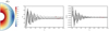 |
Fig. 2. Illustration of the unsteady phase. Left panel: meridional cut of the norm of the poloidal magnetic field. The black dots show the position of 5 control points located on different field lines. In the other two panels, the temporal evolution of these points is followed during 20τAp, both for the toroidal field Bϕc (middle panel) and the normalised differential rotation ΔΩc/Ω0 (right panel). The parameters are E = 10−4, Pr(N0/Ω0)2 = 104, Rec = 1, Lu = 5 × 10⁴, and Pm = 102 (run D5 of Table 1). |
7.2. Steady state in the viscous regime with a dipolar field
In this section we investigate, in the viscous regime and for an initial dipolar field, the steady states obtained after the Alfvén waves have dissipated and the contraction has imposed some level of differential rotation. These states are actually quasi-steady because the initial poloidal field continues to slowly decrease through magnetic diffusion. Three parameters are fixed Pr(N0/Ω0)2 = 104, E = 10−4, and Pm = 102, while the contraction Reynolds number Rec varies between 10−1 to 5, and the Lundquist number between 103 and 5 × 10⁴ (see details in Table 1). The anelastic simulations were performed with a density contrast ρi/ρ0 = 20.85.
Representative results are displayed in Fig. 3, for a case without advection of the field lines at Rec = 1 and Lu = 5 × 10⁴ (first two panels, run D5 of Table 1), and for a case with advection at Rec = 1 and Lu = 104 (last two panels, run D13 of Table 1). From this figure we clearly distinguish two magnetically decoupled regions with different levels of differential rotation. In the first region, the poloidal field lines are connected to the outer sphere and the flow is in quasi-solid rotation. In the second region, either the poloidal field lines loop-back on themselves inside the spherical shell (case without advection of the field lines) or they loop-back on the inner sphere (case with advection of the field lines). As in Charbonneau & MacGregor (1993), we shall refer to these particular regions as the ‘dead zone’ (DZ). The level of differential rotation is always significant in the DZs. With contraction of the field lines, the maximum differential rotation max(δΩ(r,θ)/Ω0) = max((Ω(r,θ)−Ω0)/Ω0) is 30%, while it is reduced to ∼1% in the other case. The snapshots of the toroidal magnetic field (second and fourth panels in Fig. 3), show the presence of two anti-symmetric lobes of toroidal field in both hemispheres due to the Ω-effect acting on the dipolar poloidal field. Interestingly, the DZs are surrounded by a region of strong toroidal field. This corresponds to a Shercliff boundary layer (Shercliff 1956) that develops between two magnetic regions that are forced to rotate at different rates. Indeed, in our simulations the first poloidal line delimiting the DZ and the neighbouring lines connected to the outer sphere are forced to rotate differentially and a layer involving strong toroidal fields accommodates this jump in rotation rate. We verified that, as expected (Roberts 1967), the thickness of this Shercliff boundary layer scales with the inverse of the square root of the Hartmann number defined by  . When we prevent the advection of the field lines (first panel in Fig. 3), a second Shercliff layer is visible at the separation between the region where the field lines are connected to both the outer and inner spheres, and the region where they are connected to the outer sphere only.
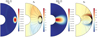 |
Fig. 3. Meridional cuts of the rotation rate normalised to the value at the outer sphere (first and third panels) and toroidal field (second and fourth panels), in the quasi-steady state. In black lines are also represented the poloidal field lines (first and third panels) and the streamlines associated with the electrical-current function defined in Appendix A (second and fourth panels). The dotted (solid) lines then correspond to an anticlockwise (clockwise) current circulation. In the first two panels, the contraction does not advect the poloidal field lines and the quasi-steady state is achieved after ∼0.04τc (i.e. ∼ 20τAp, see Fig. 2). In the last two panels such an advection is allowed and the quasi-steady configuration is reached after ∼1τc (i.e. after ∼100τAp for this simulation). For these two cases, the Lundquist numbers are respectively Lu = 5 × 10⁴ and Lu = 104 (runs D5 and D13). The other parameters are identical, namely Pr(N0/Ω0)2 = 104, E = 10−4, Rec = 1, and Pm = 102. |
To give a more detailed description of the dynamics outside and inside the DZ, we compare in Fig. 4 the relative amplitudes of the different terms of the AM balance Eq. (11). From the first two panels of this figure, we see that outside the DZ, the quasi-steady configuration is characterised by a balance between the contraction term and the Lorentz force, that is:
![$$ \begin{aligned} \! -2 \sin {\theta }\, \Omega _0 \displaystyle \frac{V_0 r_0^2}{r^2}\!\! =\!\! \displaystyle \frac{1}{\mu _0 \rho _0} \! \left[\displaystyle \frac{B_{\theta }}{r \sin {\theta }} \displaystyle \frac{\partial }{\partial \theta } \left( \sin {\theta } B_{\phi } \right) + \displaystyle \! \frac{B_r}{r} \displaystyle \frac{\partial }{\partial r} \left( r B_{\phi } \right) \right]. \end{aligned} $$](/articles/aa/full_html/2022/05/aa41613-21/aa41613-21-eq53.gif)
 |
Fig. 4. 2D maps comparing the relative importance of different azimuthally projected quantities: the Lorentz force with the contraction (first two panels) and the viscous term with the contraction (last two panels). The runs where the contraction term has been removed from the induction equation are presented in the first and third panels. In the other two, the effect of the contraction on the magnetic field is taken into account. The parameters are the same to those of Fig. 3. |
On the contrary, the last two panels of Fig. 4 show that inside the DZ the viscous term balances the contraction term, thus leading to
![$$ \begin{aligned}&\nu \left[r \displaystyle \frac{\partial ^2}{\partial r^2} \left( \displaystyle \frac{\delta \Omega }{\Omega _0} \right) + 4 \displaystyle \frac{\partial }{\partial r} \left( \displaystyle \frac{\delta \Omega }{\Omega _0} \right) + \displaystyle \frac{1}{r} \displaystyle \frac{\partial ^2 }{\partial \theta ^2} \left( \displaystyle \frac{\delta \Omega }{\Omega _0} \right) + \displaystyle \frac{3 \cot {\theta }}{r} \displaystyle \frac{\partial }{\partial \theta } \left( \displaystyle \frac{\delta \Omega }{\Omega _0} \right) \right]\nonumber \\&\quad = \displaystyle \frac{-2 V_0 r_0^2}{r^2} , \end{aligned} $$](/articles/aa/full_html/2022/05/aa41613-21/aa41613-21-eq54.gif)
where only the linear part of the contraction term has been retained, an approximation only valid if δΩ/Ω0 ≪ 1. In the following two sub-sections, the differential rotation resulting from these two different balances is analysed.
7.2.1. Region outside the dead zone
Although at first glance the flow seems to be in solid rotation outside the DZ, there is a rotation rate jump across a boundary layer at the outer sphere as well as a residual differential rotation along the poloidal field lines.
By rescaling the colour range of Fig. 3, the top panel of Fig. 5 indeed shows that outside the DZ, the differential rotation between the interior flow and the outer sphere (Ω(r,θ)−Ω0)/Ω0) is ∼6 × 10⁻⁴. In order to understand that value, we first estimate the toroidal field amplitude outside the DZ using Eq. (34). Assuming Br ∼ Bθ ∼ B0 and r ∼ r0, we get
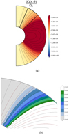 |
Fig. 5. Normalised rotation rate in the quasi-steady state. Top panel (5a): this is the third panel of Fig. 3 presented on a smaller rotation rate scale. As a result, the DZ is saturated in colour. Bottom panel (5b): enlargement of the black-delimited zone displayed in the top panel. In each panels, the poloidal field lines are also represented (black lines). For the sake of clarity, every other field line is plotted in red in the bottom panel. The parameters are the same as in Figs. 3 and 4. |
This estimate is confirmed in Fig. 6 where Bϕ/B0 determined at a particular location, θ = π/6, r = 0.65r0, is compared with the right-hand side of Eq. (36) for the runs D1–D7.
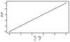 |
Fig. 6. Toroidal field Bϕ normalised to the initial amplitude of the poloidal field B0, as a function of (Pm/Lu)2Rec/E and at the particular location θ = π/6 and r = 0.65r0. The different symbols correspond to the different runs D1–D7 of Table 1 (no contraction term in induction equation) namely, Rec = 10−1, Lu = 104 (circle); Rec = 10−1, Lu = 5 × 10⁴ (square); Rec = 1, Lu = 5 × 10³ (hexagon); Rec = 1, Lu = 104 (up triangle); Rec = 1, Lu = 5 × 10⁴ (pentagon); Rec = 5, Lu = 104 (down triangle) and Rec = 5, Lu = 5 × 10⁴ (diamond). The other parameters are fixed to E = 10−4, Pr(N0/Ω0)2 = 104, and Pm = 102. |
This toroidal field is however unable to naturally match the vacuum condition imposed at the outer sphere (Bϕ = 0 at r = r0). This is done across a  thickness magnetic boundary layer known as an Hartmann boundary layer. This layer is analysed in Appendix B and the conclusion is that the
  jump on Bϕ/B0, induces a
  jump on the differential rotation ΔΩ/Ω0 across the layer. This last scaling is confirmed in Fig. 7 by computing ΔΩ/Ω0 at a particular location for the runs D1–D7.
 |
Fig. 7. Normalised differential rotation between a point outside the DZ and the outer sphere, ΔΩ/Ω0 = (Ω(r = 0.65r0,θ=π/12)−Ω0)/Ω0, plotted as a function of |

Figure 5b shows a zoom on the zone delimited in black lines in Fig. 5a. It illustrates the residual differential rotation that exists along each poloidal field lines. We note it as ΔΩpol/Ω0. Such a contrast of differential rotation is at odds with Ferraro’s law of isorotation (Ferraro 1937) requiring a constant angular velocity along each poloidal field line. Ferraro’s isorotation state is indeed found in our cases with no contraction in the induction equation. However, taking field advection into account, the Ω-effect term can be balanced by the radial advection term in the induction equation, that is:
Using the order of magnitude of the toroidal field derived in Eq. (36) together with Eq. (37), we end up with an estimate of this differential rotation
Figure 8 shows the differential rotation taken between two ends of a poloidal field line as a function of the right-hand side of Eq. (38), for various Rec and Lu respectively ranging from 10−1 to 2 and from 5 × 10³ to 104. We can see that the level of differential rotation along a field line is indeed consistent with our estimate.
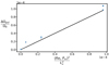 |
Fig. 8. Normalised differential rotation along a poloidal field line ΔΩpol/Ω0 as a function of (RecPm/Lu)2. This quantity is estimated between two sufficiently separated points along a field line for the runs D8 and, D10–D14 of Table 1. The correspondences between parameters and symbols are as follows: circle: Rec = 10−1, Lu = 104; triangle: Rec = 5 × 10⁻¹, Lu = 5 × 10³; diamond: Rec = 5 × 10⁻¹, Lu = 104; square: Rec = 1, Lu = 5 × 10³; pentagon: Rec = 1, Lu = 104; hexagon: Rec = 2, Lu = 104. The other parameters are E = 10−4, Pr(N0/Ω0)2 = 104, and Pm = 102. |
Another consequence of the force balance Eq. (34) is that the toroidal field amplitude slowly increases over time. Figure 9 illustrates this by showing that in order to counteract the magnetic diffusion of the poloidal field (blue curve) and maintain this balance (black curve), the toroidal field amplitude is forced to increase (green curve). A similar situation was reported by Charbonneau & MacGregor (1993) where the magnetic stresses were in their case balanced by a wind torque.
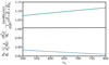 |
Fig. 9. Temporal evolution of different quantities followed over a period of 300τAp: the toroidal field normalised to the initial amplitude of the poloidal field and rescaled by |

7.2.2. Dead zone
We now turn to investigate the dynamics of the DZ. We already found that in this region, the dominant balance is between the contraction and the viscous effects, and is given by Eq. (35) in the linear regime ΔΩ/Ω0 ≪ 1. This implies that the order of magnitude of the differential rotation in the DZ, denoted ΔΩDZ/Ω0, is ∼LDZVf(r)/ν, where LDZ is a typical lengthscale of the DZ. While the magnetic field does not explicitly enter in this expression, it is of prime importance because its interaction with the contraction determines the shape and the location of the DZ.
The differences observed in Fig. 3 concerning the level of differential rotation between the simulations with and without contraction of the field lines can thus be explained by the location and size of the DZ. Indeed, in the case without field line contraction, the DZ is smaller and located closer to the outer sphere, that is in a area where the contraction velocity is weaker, which leads to a smaller level of differential rotation. Another difference between these two cases is the time taken to reach the stationary solution. As this time is the viscous time based on the size of the DZ, it is not surprising that the stationary state is reached much more rapidly when the DZ occupies a small fraction of the spherical shell. We note that in the case with contraction of the field lines, the viscous time is of the same order as the contraction time τc because we are in the regime ΔΩ/Ω0 ∼ 1.
It is also possible to obtain a more precise determination of the DZ differential rotation, by deriving an approximate analytical solution of Eq. (35). To this end, the DZ is first assimilated to a conical domain, r ∈ [riDZ,r0], θ ∈ [ − θ0, θ0], outside of which the flow is in solid rotation. In the case where the domain connects to the inner sphere, we adopt a stress-free condition on the azimuthal component of the velocity field at r = ri. We then neglect the last term of the left-hand side in Eq. (35) as we found in our simulations that its contribution is small, particularly at low latitude. The homogeneous problem, which is separable in two radial and latitudinal eigenvalue sub-problems, allows us to construct a basis of orthogonal eigenfunctions that satisfy the boundary conditions on the conical domain. The details of the method are provided in Appendices C.1 and C.2.
In the case where the contraction does not advect the field lines, the approximate analytical solution takes the following form
wherein the expression of the coefficient Ank can be found in Appendix C.1. This solution, computed for a chosen conical domain, is compared in Fig. 10 with the results of the numerical simulations performed at various Rec and Lu respectively ranging from 10−1 to 5 and from 5 × 10³ to 5 × 10⁴. A good agreement is found between the numerical and analytical solutions. The differential rotation scales as Rec and this was expected because the condition δΩ/Ω0 ≪ 1 for the linear approximation of the contraction term is fulfilled in the simulations. We also find that the differential rotation is almost independent of the initial amplitude of the magnetic field: an increase of Lu of one order of magnitude causes only a small change on ΔΩDZ/Ω0. This is consistent with the fact that, in the regime considered here, the shape and location of the DZ do not depend on the magnetic field. We rather observe that a higher magnetic field affects the rotation rate outside the DZ, or equivalently the differential rotation outside the DZ. Again this is expected as the jump in rotation rate across the outer sphere Hartmann layer decreases with the field amplitude.
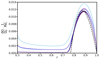 |
Fig. 10. Equatorial differential rotation as a function of radius when the contraction term is removed from the induction equation. Numerical solutions (runs D1–D7) are plotted in colour at Rec = 10−1 (red), Rec = 1 (blue), and Rec = 5 (purple), for various Lundquist numbers ranging from 104 to 5 × 10⁴ (from the lightest to the darkest). For Rec = 1, an additional simulation is presented at Lu = 5 × 10³. The curves are rescaled by Rec then compared to the analytical solution Eq. (39) displayed in black dashed lines. The other parameters are E = 10−4, Pr(N0/Ω0)2 = 104, and Pm = 102. |
When the contraction term is introduced in the induction equation, the solution of Eq. (35) becomes
where the expressions of the coefficients Ank and μn are given in Appendix C.2. This solution, computed for a chosen conical domain, is compared in Fig. 11 with the numerical results obtained at various Rec and Lu. As previously, the initial amplitude of the magnetic field causes only small changes on the level of differential rotation. However, some discrepancies are visible. First of all, the numerical curves obtained at different Rec do not overlap, which indicates that for these higher levels of differential rotation (δΩ/Ω0 ∼ 30%) the contraction term can no longer be linearised, a necessary condition to derive the analytical solution. A second limitation is the assumed conical shape of the DZ. This shape is indeed more representative of the actual DZ for run D14 performed at Rec = 2, where we can observe that the analytical solution tends to reproduce the expected differential rotation, than for simulations D10–D13 obtained at Rec = 0.5 and 1.
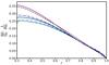 |
Fig. 11. Same as Fig. 10 but for cases where contraction acts on the field lines. The simulations presented here are the runs D10–D14 of Table 1 performed at Rec = 5 × 10⁻¹ (green), Rec = 1 (blue), and Rec = 2 (purple). For all these cases Lu = 104, but for Rec = 5 × 10⁻¹ and 1, additional simulations are shown at Lu = 5 × 10³ in dash-dot lines. The analytical solution Eq. (40) is displayed in black dashed lines. |
7.2.3. Effect of the density stratification
We have performed simulations in the anelastic approximation for a fixed density contrast ρi/ρ0 = 20.85. Two typical results are presented in Fig. 12 at Rec = 1, Lu = 105 and Rec = 5, Lu = 5 × 10⁴ (left and right panels respectively). For these runs where the contraction advects the field lines, we find again two separate regions, with a differential rotation still mostly located in the DZ. This zone is now more extended in latitude compared to the Boussinesq case and the main difference between the calculations at two different Rec lies in the level of differential rotation in the DZ. Indeed, when this level in the left panel is compared to its Boussinesq counterpart in the third panel of Fig. 3, we notice that it has been divided by a factor ∼3. This is explained by the density stratification effect on the contraction velocity field. Indeed, as we already found in Gouhier et al. (2021), the normalised differential rotation ΔΩDZ/Ω0 resulting from the balance between the viscous and contraction effects is weighted by the inverse of the background density profile:
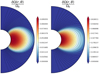 |
Fig. 12. Meridional cuts of the normalised rotation rate in two anelastic cases with ρi/ρ0 = 20.85. The poloidal field lines are represented in black lines. For these simulations the contraction term is included in the induction equation. In the first panel, Rec = 1 and Lu = 105 (run D18 of Table 1). In the second one, Rec = 5 and Lu = 5 × 10⁴ (run D20 of Table 1). The other parameters are Pr(N0/Ω0)2 = 104, E = 10−4, and Pm = 102. |
where the index A stands for ‘anelastic’ and B for ‘Boussinesq’. For ρi/ρ0 = 20.85 and r ∈ [ri = 0.3;r0 = 1], using the characteristic amplitude of the differential rotation given in the third panel of Fig. 3, we obtain  , in agreement with the rotation rate shown in the left panel of Fig. 12. A good estimate of the rotation rate displayed in the right panel is then readily obtained by multiplying this result by Rec.
7.3. Quadrupolar field in the viscous regime
We now consider an initial quadrupolar magnetic field as given by Eq. (23) and displayed in the right panel of Fig. 1. The outcome will be completely different as the differential rotation resulting from the contraction is subject to an instability that will be discussed in detail below.
Figure 13 displays typical states obtained after a contraction timescale. The two left panels show a case without contraction of the field lines while the two right panels correspond to simulations where contraction is included in the induction equation. At this stage, the similarities with the dipolar case are striking. First, we observe the quasi-solid rotation region outside the DZs. When the advection of the field lines is prevented, these DZs are located near the outer sphere while they connect to the inner sphere when contraction is present. In addition, for a given set of parameters, when the dipolar and quadrupolar cases are compared with each other, the same levels of differential rotation are found. For the runs presented here, the maximum amplitude of the normalised differential rotation inside the DZs is again ∼30% when the contraction acts on the field lines, and falls to ∼1% otherwise, similar to the cases presented in Fig. 3. By observing the second and fourth panels of Fig. 13, we note, again, the presence of magnetic boundary layers namely, the Shercliff layers separating the poloidal field lines constrained to rotate at different rates, and the Hartmann layer at the outer sphere. However, compared to the dipolar case, after ∼1τc the quadrupolar configuration is the seat of an axisymmetric instability.
 |
Fig. 13. Same as Fig. 3, but for the initially quadrupolar magnetic field. In the first two panelsLu = 5 × 10⁴, while Lu = 104 in the last two. The other parameters are Rec = 1, E = 10−4, Pr(N0/Ω0)2 = 104, and Pm = 102 (runs Q2 and Q10 of Table 1). |
The evolution of the maximum differential rotation is shown in Fig. 14 where the different steps that will be described thereafter are highlighted. In particular, the differential rotation first builds up before an instability starts to kick in at t ∼ 1τc (red dashed lines). Between ∼1τc and ∼3.5τc (blue dashed lines), the instability grows, saturates and strongly modifies the flow and field as we shall see later. Finally, after 3.5τc, the configuration evolves more smoothly until a final steady state is reached at ∼4.7τc (purple dashed lines).
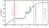 |
Fig. 14. Maximum value of the normalised differential rotation max(ΔΩ/Ω0) as a function of the contraction timescale as defined in Eq. (12). The main evolution steps are highlighted by coloured dashed lines: the red dashed lines corresponds to the start of the exponential growth phase and orange, to the time at which the instability saturates, thus marking the beginning of the non-linear evolution. Then, blue marks the start of the post-instability evolution and finally, purple denotes the time at which the hydrodynamic steady state is reached. The parameters are Rec = 1, Lu = 104, E = 10−4, Pr(N0/Ω0)2 = 104, and Pm = 102 (run Q10 of Table 1, contraction term in induction equation). |
7.3.1. Description of the instability
Figure 15 shows, in colour, the structure of the unstable modes when the contraction does not act on the field lines (first panel) and when it acts on them (second panel). In these meridional cuts are also represented, in black, the contours of the latitudinal shear ∂lnΩ/∂θ. Dashed (solid) lines represent negative (positive) values of this gradient. Contrary to the dipolar case, we now have a region of negative shear in the northern hemisphere and positive shear in the south. As can be observed, this is precisely at these locations that the perturbations grow. We already note that this instability is not of the centrifugal type because the shear in these regions is not strong enough, that is |∂lnΩ/∂lns| < 2. Figure 15 also shows that the unstable modes are characterised by small radial length scales and large horizontal length scales, which implies that the meridional motions are predominantly horizontal. The last panel of Fig. 15 displays the local evolution of the square of the latitudinal component of the velocity field at the fixed points marked on the second panel (in light blue, blue and black). We can see that the kinetic energy of the perturbations grows exponentially for about ∼20τAp before saturation occurs. This time interval corresponds to the linear phase of the instability. The oscillating behaviour that adds to the exponential growth is due to the fact that the perturbations propagate.
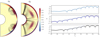 |
Fig. 15. Axisymmetric instability in the viscous regime when the quadrupolar field given by Eq. (23) and illustrated in Fig. 1, is initially imposed. First two panels: snapshots of the latitudinal component of the velocity field Uθ taken during the developing of the instability, at t = 14.1τAp when the contraction does not act on the field lines (first panel) and at t = 127.4τAp when it does (second panel). In these cuts are also represented the contours of the latitudinal shear ∂lnΩ/∂θ in black, with dashed lines corresponding to a negative shear and full lines to a positive one. In the second panel, three control points (in light blue, blue and black) are chosen at the location where the instability grows. Third panel: temporal evolution of the square of the latitudinal component of the velocity field at these selected points (with the same colour code), as a function of the Alfvén poloidal time. In each subplot, a coloured straight line is also presented as the result of a linear regression used to deduce a growth rate associated with the instability. The parameters are those of the runs Q4 and Q10 of Table 1 namely, Rec = 5 (first panel) and Rec = 1 (two last panels), with E = 10−4, Pr(N0/Ω0)2 = 104, Pm = 102, and Lu = 104. |
Growth rates have been determined from these plots. Their values, normalised by the product of the surface-averaged shear parameter ⟨q⟩ = 1/S∬(∂lnΩ/∂θ)dS to the mean local rotation rate, are listed in Table 2. We observe that when the contraction Reynolds number is multiplied by two, the shear rate and the growth rate are both doubled. This shows that the growth rate of the instability seems to be proportional to the shear rate. Moreover, for the simulation Q5 performed at higher Lu = 5 × 10⁴, the instability is not triggered, clearly indicating that a strong enough poloidal field has a stabilising effect. Finally, while runs Q4, Q10 and Q11 carried out for Lu = 104 are unstable, runs Q1 and Q8 performed for the same Lu, but at lower Rec, are stable. This shows that, at a lower shear rate, a lower poloidal field is required to stabilise the flow. These findings, namely the requirement that the rotation decreases away from the rotation axis, and the facts that the growth rates are proportional to the shear and that stabilisation occurs above a certain magnetic tension, are all in agreement with an MRI-type instability (Balbus & Hawley 1991).
Ratio between the growth rate σi = 1, 2, 3 of the instability and the product of the absolute value of the surface-averaged shear parameter |⟨q⟩| by the local rotation rate Ω.
Our numerical results also exhibit more subtle effects that are not accounted for in the local WKB approach of the standard MRI (SMRI) (Balbus & Hawley 1991, 1994; Menou et al. 2004). First, the growth rates determined in Table 2 are significantly lower than the maximum growth rate σmax = |q|Ω/2, where q = dlnΩ/dlns, predicted by these studies (e.g. Balbus & Hawley 1994). Second, a comparison between runs Q9 and Q10 shows that the growth rate increases with Lu whereas the predicted σmax does not depend on the poloidal field. Finally, as noted earlier, the perturbations propagate in the domain while the phase velocity of the modes is zero in the SMRI.
We now argue that these differences are due to the effect of the stable stratification and to the presence of a toroidal field. In Balbus & Hawley (1994), the maximum growth rate is determined by assuming a zero latitudinal wavenumber. This avoids any stabilising effect of the stratification because the buoyancy force has no effect on purely horizontal motions. It follows that the most unstable radial scale is inversely proportional to the poloidal field amplitude and does not depend on the stable stratification. Even if the unstable motions found in our simulations are predominantly horizontal, assuming a zero latitudinal wavenumber is too extreme because our background flow is not uniform in latitude, so that the perturbation must have, and indeed, has a finite wavelength in this direction. As a consequence, the stable stratification is expected to play a role in determining the most unstable radial lengthscale and the associated maximum growth rate. We indeed found that the radial wavenumbers of the unstable modes are always larger the theoretical value from Balbus & Hawley (1994) and that it is very little dependent on the amplitude of the poloidal field. The effect of the stable stratification may thus potentially explain why the growth rates found in our simulations are significantly smaller than σmax. We note that the thermal diffusion must be taken into account to consider the effect of the stable stratification. Indeed, we estimated that the thermal diffusion time scale  associated with the observed unstable modes is about one order of magnitude smaller than the buoyancy time scale
  , which implies that thermal diffusion will play an important role in determining the amplitude of the buoyancy force (e.g. Lignières et al. 1999).
To interpret the increase of the growth rate with Lu (runs Q9 and Q10), we first recall that in the context of the SMRI the toroidal field is assumed to be zero. This is not the case in our simulations where, according to Eq. (34), the amplitude of the stationary toroidal field decreases when the initial poloidal field (and thus Lu) increases. As reviewed in Rüdiger et al. (2018), introducing a toroidal field leads to the so-called helical MRI (HMRI) (Hollerbach & Rüdiger 2005). Following the dispersion relation derived by Kirillov et al. (2014), the toroidal field can be either stabilising or destabilising depending on the sign of  . Moreover, the HMRI differs from the SMRI through the non-vanishing phase velocity of the unstable modes and a different phase shift between the perturbed fields. This phenomenon has been mentioned for the first time by Knobloch (1992), then found experimentally by Stefani et al. (2006) and in numerical simulations by Petitdemange et al. (2013).
In our simulations, the quantity VAϕ/s changes sign in the region where the instability is triggered so that the WKB-type analysis of Kirillov et al. (2014) is not directly conclusive. Our results nevertheless would imply that the toroidal field has a stabilising effect since the growth rate increases when the intensity of Bϕ decreases. As noted earlier, we did observe that the perturbations propagate in our simulations. Their phase velocity Vphase, normalised by the contraction velocity field, are listed in Table 3. As expected, comparing the runs Q9 and Q10, we observe that the phase velocity is higher when the toroidal field is higher. Moreover, contrary to a SMRI, we observe neither exact phase quadrature between the latitudinal velocity perturbation and the latitudinal and azimuthal magnetic perturbations, nor exact opposition phase between the perturbed latitudinal and toroidal magnetic fields (Petitdemange et al. 2013). This is visible in Fig. 16 where the different perturbed quantities, the latitudinal velocity (purple) as well as the latitudinal (green) and azimuthal (blue) magnetic fields, are plotted as a function of the radius.
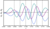 |
Fig. 16. Perturbed fields: latitudinal component of the velocity field (purple), and latitudinal (green) and azimuthal (blue) components of the magnetic field, as a function of radius at θ ≈ 2π/5 (i.e. at latitude π/10). The parameters are Rec = 1, Lu = 104, E = 10−4, Pr(N0/Ω0)2 = 104, and Pm = 102 (run Q10 of Table 1). |
We conclude that the instability triggered in the DZ of the quadrupole is of the MRI-type and that its full description would require a detailed modelling of the effects of the stable stratification and of the toroidal field.
7.3.2. Non-linear evolution
After the exponential growth phase, the evolution becomes non-linear and the instability saturates. Figure 17 displays the flow structure obtained at ∼3τc for the run Q10 (Rec = 1, Lu = 104), through the rotation rate (colour) and the meridional circulation (black) in the left panel, as well as the norm of the poloidal field (colour) and its associated field lines (black) in the right panel. We observe that the instability proceeds via a multi-cellular meridional circulation, radially confined by the stable stratification and latitudinally extended in both hemispheres. From Fig. 17, we see that the poloidal field lines (right panel) are dragged around by this meridional circulation everywhere it is present (left panel), and then warped. The poloidal field thus behaves like a passive scalar advected and mixed by the multi-cellular circulation. This process creates small scales on which the magnetic diffusion can efficiently act to dissipate the poloidal field.
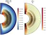 |
Fig. 17. Structure of the flow and of the magnetic field during the non-linear evolution. Left panel: meridional cut of the normalised differential rotation δΩ/Ω0 (colour) with the streamlines associated with the meridional circulation U = Urer + Uθeθ (black contours). The dashed (solid) lines correspond to an anticlockwise (clockwise) circulation. Right panel: meridional cut of the normalised norm of the poloidal magnetic field ∥Bp∥/B0 (colour) and its associated field lines (in black). The fixed point, located at r = 0.47r0 and θ ≈ 2π/5, corresponds to the location where the norm of the poloidal field is plotted in Fig. 18 for a stable and an unstable case. These snapshots have been taken at t = 3τc. The parameters are Rec = 1, Lu = 104, E = 10−4, Pr(N0/Ω0)2 = 104, and Pm = 102 (run Q10 of Table 1). |
In Fig. 18, we compare the evolution of the norm of the poloidal field in an unstable case (in black) and in a stable case (in blue). The field norm is determined either through a volume average (solid line) or at a fixed point (displayed in black in Fig. 17) in the middle of the unstable region (dashed lines). The slope of these curves enables us to estimate a diffusion rate, and so a diffusion lengthscale, of the poloidal field. For the unstable configuration, this rate is determined during the saw-tooth evolution ranging from ∼2.25τc to ∼3.5τc. By denoting  and
and  the diffusion rates of the stable and unstable runs respectively, we obtain ωunst/ωstab ≈ 42, hence a diffusion of the poloidal field 42 times faster in the unstable case. In other words, the motions driven by the instability induce an effective diffusion at a lengthscale 6.5 smaller than the diffusion acting in the stable case (Lstab/Lunst = 6.5).
 |
Fig. 18. Temporal evolution of the norm of the poloidal magnetic field normalised to B0, as a function of the contraction timescale τc. Plain curves represent a volume-averaged evolution and dashed-dotted ones, a local evolution at the fixed point displayed in black in Fig. 17 (r = 0.47r0 and θ ≈ 2π/5). The stable and unstable configurations, Rec = 0.5 and 1, are respectively distinguished by their blue and black colours. The other parameters are E = 10−4, Pr(N0/Ω0)2 = 104, Pm = 102, and Lu = 104 (runs Q8 and Q10 of Table 1). |
Although we shall see below that the differential rotation increases as a result of the instability, the toroidal field does not grow through the Ω-effect because the poloidal field is too weak in this phase. Then, the toroidal field experiences a diffusive-like decay, similar to the poloidal field.
7.3.3. Post-instability description
By destroying the poloidal field, the instability allowed a reconfiguration of the flow structure. This is shown at t = 3.5τc in the first two panels of Fig. 19, then at t = 4.66τc in the last two. From the first panel, we observe that the maximum level of differential rotation is now three times higher than before the instability. The reason is as follows: from a DZ to another, the large-scale structure of the poloidal field has been destroyed by the instability. As a result, even if a significant level of toroidal field still exists in this region, as displayed in the second panel of Fig. 19, the Lorentz force remains weak between the two DZs. The domain within which the contraction is balanced by the viscous effects thus becomes larger and, as expected, the differential rotation increases. By contrast, the poloidal field amplitude is still significant near the rotation axis and the Lorentz force imposes a very weak differential rotation 𝒪((RecPm/Lu)2) (see Sect. 7.2.1) in this region.
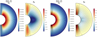 |
Fig. 19. Meridional cuts of the normalised differential rotation δΩ/Ω0 and of the toroidal field Bϕ, obtained during the post-instability evolution at ∼3.5τc (first two panels), and when the hydrodynamic steady state is reached at ∼4.66τc (last two panels). Black contours represent either the poloidal field lines (first and third panels) or the streamlines associated with the electrical-current function (second and fourth panels). The parameters are E = 10−4, Pr(N0/Ω0)2 = 104, Pm = 102, Rec = 1, and Lu = 104 (run Q10 of Table 1). |
Coming back to the numerical results presented in Fig. 19. The first two panels show that the magnetic topology has also completely changed after the development of the instability. A comparison between the third panel of Fig. 13 and the first panel of Fig. 19 shows that the field lines which looped back on themselves before the instability have now been moved towards the poles. In addition, the toroidal field is now very weak close to the outer sphere. An Hartmann layer is thus no longer needed to connect to the vacuum condition at the outer sphere. Likewise, the Shercliff layers have been removed with the dissipation of the poloidal field. Interestingly, we note that the new magnetic configuration, characterised by its positive lobe of toroidal field located near the rotation axis in both hemispheres, is from now on likely to be unstable to a non-axisymmetric instability of Tayler-type (see e.g. Spruit 1999).
After ∼4.66τc, the third panel of Fig. 19 shows that the differential rotation is mostly radial and occupies the whole shell. As a consequence, its amplitude further increased. In Fig. 20, we plotted in black dashed line the analytical solution corresponding to the balance on the full sphere between the viscous and contraction terms of Eq. (11). This solution, derived in Gouhier et al. (2021), perfectly matches the numerical solution in blue, thus showing that the hydrodynamic steady state is recovered. In conclusion, the magnetic field now has a negligible effect on the flow dynamics as supported by the fourth panel of Fig. 19 where we can see that the amplitude of the toroidal field has been divided by more than 10.
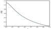 |
Fig. 20. Normalised differential rotation δΩ/Ω0 as a function of radius. The analytical solution derived by solving the balance between the viscous and contraction terms in Eq. (11), is plotted in black dashed lines. It is compared to the numerical solution obtained at 4.66τc and plotted in blue solid line. The parameters used are the same as in Fig. 19. |
7.4. Steady state in the Eddington–Sweet regime
We now focus on the Eddington–Sweet regime ( ) considering a dipolar or a quadrupolar field as the pre-existing field. All simulations were performed in the anelastic approximation and included the contraction term in the induction equation. The contrast of density between the inner and the outer spheres was fixed to 20.85, and the Ekman and magnetic Prandtl numbers were respectively equal to 10−5 and 102. Our parametric study in this regime study consists in varying Rec from 10−1 to 5 and Lu from 5 × 10³ to 105 for Pr(N0/Ω0)2 = 10−2 and 10−1 (see details in Table 1).
We basically found three types of steady states. The first one is characterised, as in the viscous case, by two magnetically decoupled regions, one of them including a DZ where the contraction enforces a certain level of differential rotation. This state is the most relevant in a stellar context because it is obtained for the lowest values of τAp/τED and τAp/τc, and these ratios are a priori very small in magnetic contracting stars as discussed in Sect. 6.1. As we increase these ratios, we find another type of solution where the differential rotation and the meridional circulation are no longer confined within the DZ while the field topology is unchanged (for higher τAp/τED), and finally a state where the advection of the poloidal field destroys the DZ and significantly reconfigures the magnetic field and the rotation profile (for higher τAp/τc). In the following, these last two solutions will be described briefly as they are thought to be less relevant for our purpose, although physically interesting.
7.4.1. Meridional circulation and differential rotation confined to the dead zone
Figure 21 displays the typical structure of the quasi-steady flows and fields obtained for a dipolar (top row) or a quadrupolar (bottom row) initial field. These simulations were performed at Rec = 1, Lu = 105 and Pr(N0/Ω0)2 = 10−1 (runs D28 and Q13 of Table 1), and thus satisfy τAp/τED = 10−2 and τAp/τc = 10−3. There are many similarities with the viscous case. From the panels of the first column, we again observe two regions that are magnetically decoupled. One occupies the major part of the spherical shell and is in quasi-solid rotation while the other, the DZ, exhibits a certain level of differential rotation. The amplitude of this differential rotation is similar for the dipolar and quadrupolar cases. We also note the presence of magnetic boundary layers: the Hartmann layer at the outer sphere, and the Shercliff layers wherever adjacent poloidal field lines are forced to rotate differently, namely along the tangent cylinder and around the DZ. As in the viscous case, the toroidal field is characterised by a strong amplitude at these locations, as indicated by the panels of the second column.
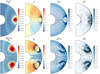 |
Fig. 21. Quasi-steady axisymmetric flow in the Eddington–Sweet regime when a dipolar (top row) or quadrupolar (bottom row) field is initially imposed. Panels of the first column: rotation rate normalised to the top value (colour) and poloidal field lines (black). Panels of the second column: toroidal field (colour) with the streamlines of the electrical-current function (black). Panels of the third column: norm (colour) and streamlines (black) of the total meridional circulation |

We also see major differences with the viscous regime. First, although the contraction of the field lines is allowed, the DZ is confined near the outer sphere, whether a dipolar or quadrupolar field is initially imposed. This can be compared to the third panels of Figs. 3 and 13 in the viscous regime where the DZ was clearly advected towards the inner sphere. This difference is attributed to the effect of the contraction-induced meridional flow which now plays a significant role in the DZ advection. This flow is illustrated in the fourth column of Fig. 21 displaying the norm (colour) and the streamlines (black) of the poloidal velocity field Up = Urer + Uθeθ. For an initial dipolar field, this circulation is characterised by the presence of one cell of anticlockwise (clockwise) circulation in the northern (southern) hemisphere. This contraction-induced flow contributes to the total meridional circulation  displayed in the third column. As seen in the two top right panels, the induced flow inside the DZ tends to oppose contraction and the resulting total circulation becomes very weak, thus preventing the inward advection of the DZ. Outside the DZ, the total meridional flow is approximately parallel to the poloidal field lines close to the outer sphere, where the contraction velocity is maximum. In the deeper regions close to the inner sphere, the advection of poloidal field lines by the weaker contraction field is balanced by magnetic diffusion.
For an initial quadrupolar field, we observe a strong circulation around the DZ while inside the DZ the flow is predominantly vertical, downwards (upwards) in the northern (southern) hemisphere. Again, away from the DZ, the contraction-induced meridional flow has only a negligible contribution to the total meridional circulation. Finally, in contrast to the viscous regime, for the parameters numerically reachable in this study, the quadrupolar configurations are stable with respect to MRI because the shear built in the DZs is not strong enough to counteract the stabilising effect of the poloidal field. By comparison, the contrast of differential rotation in run Q5 of the viscous regime is ∼130 times larger and is not even unstable despite a weaker Lu of 5 × 10⁴.
In order to understand the flow dynamics inside and outside the DZ, we now examine the force balance in the AM equation Eq. (11), as was done in the viscous regime. The force amplitudes are analysed in the 2D maps of Fig. 22 where we display the ratio of the Lorentz force (left panel) and of the Coriolis force (right panel) to the contraction. We can observe that inside the DZ, the contraction is now balanced by the Coriolis force because the toroidal component of the magnetic field tends to zero and the Lorentz force becomes negligible accordingly (see right panel of Fig. 22). This implies that
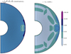 |
Fig. 22. 2D maps comparing the relative importance of the Lorentz (left panel) and Coriolis (right panel) forces to the contraction, in the presence of a dipolar field. In each panel the poloidal field lines are plotted in black. The parameters are the same as in Fig. 21. |
Here, contrary to the viscous case, the thermal diffusion weakens the stable stratification and enables a contraction-driven meridional circulation to exist. Inside the DZ, we also find that the thermal balance
![$$ \begin{aligned} U_r \displaystyle \frac{\mathrm{d} S_{m}}{\mathrm{d} r} = \kappa \left[\left( \displaystyle \frac{\mathrm{d} \ln {\overline{\rho }}}{\mathrm{d} r} + \displaystyle \frac{\mathrm{d} \ln {\overline{T}}}{\mathrm{d} r} \right) \displaystyle \frac{\partial \delta S}{\partial r} + \boldsymbol{\nabla }^2 \delta S \right], \end{aligned} $$](/articles/aa/full_html/2022/05/aa41613-21/aa41613-21-eq87.gif)
and the thermal wind balance
are both satisfied. In these expressions,  where
where  is the spherically symmetric entropy field induced by the contraction, and δS(r, θ) = S′(r, θ)−Sc(r) (see Gouhier et al. 2021 for details). According to Eq. (42), contraction then drives a meridional circulation Us ∼ 𝒪(Vf) which redistributes AM on an Eddington–Sweet timescale. We note that the circulation timescale τc can be quite different from the Eddington–Sweet timescale. Indeed, as stated in Sect. 3, the ratio τED/τc is measured by the dimensionless quantity RecPr(N0/Ω0)2. In this numerical study of the Eddington–Sweet regime, τED ≪ τc because Pr(N0/Ω0)2 ≪ 1 and because large contraction Reynolds numbers are too difficult to reach numerically.
Outside the DZ, the timescale of AM transport by the Alfvén waves is much shorter than the Eddington–Sweet timescale, and the Alfvén waves impose their dynamics. The left panel of Fig. 22 thus shows that the Lorentz force balances the contraction and Eq. (34) holds, as in the viscous regime. In this case, a quasi-isorotation state along the field lines is obtained, verifying:
![$$ \begin{aligned} V_{f}(r) \left[\displaystyle \frac{\partial }{\partial r} \left( \displaystyle \frac{B_{\phi }}{r} \right) - \displaystyle \frac{B_{\phi }}{r} \displaystyle \frac{\mathrm{d} \ln {\overline{\rho }}}{\mathrm{d}r} \right]= \sin {\theta } \left( \boldsymbol{B}_p \times \boldsymbol{\nabla } \right) \delta \Omega . \end{aligned} $$](/articles/aa/full_html/2022/05/aa41613-21/aa41613-21-eq91.gif)
As a result, the estimate of the characteristic amplitude of the differential rotation along the field lines Eq. (38) still holds, except that it must be weighted by  accounting for the effect of the density stratification in the domain.
In the hydrodynamical case (Gouhier et al. 2021), we showed that the characteristic amplitude of the steady differential rotation resulting from the balance between the inward AM transport by the contraction and the AM redistribution by the Eddington–Sweet circulation should be  . This global analysis does not apply directly in the present situation where the DZ is reduced to a small fraction of the spherical shell, confined near the outer sphere. As in Sect. 7.2.2, and following Oglethorpe & Garaud (2013), to account for the DZ size and its effect on the differential rotation induced by the Eddington–Sweet circulation, we introduce the lengthscale LDZ = 0.1r0. Because of the density stratification, the contraction velocity is not very different between the outer and inner spheres. Thus, after using Eq. (42) and the continuity equation, we have Ur ≈ V0. Then, from Eq. (43) we get
  . Injecting this estimate in Eq. (44) yields finally to
  , thus enabling us to recover the level of differential rotation inside the DZ up to a factor two.
In Fig. 23, we plotted the maximum amplitude of the differential rotation inside the DZ as a function of Pr(N0/Ω0)2Rec, for the runs D21–D24 and D27–D30 of Table 1 performed with Rec ranging from 10−1 to 2 (identified with symbols) and Lu from 5 × 10⁴ (light blue) to 105 (blue). The other parameters are fixed to Pr(N0/Ω0)2 = 10−1, E = 10−5, Pm = 102, and ρi/ρ0 = 20.85. As expected, the maximum contrast of differential rotation follows a linear relation with Rec. Moreover, we also observe that this level is almost independent of the Lundquist number, consistent with the balance Eq. (42) inside the DZ. However, for the highest contraction Reynolds number Rec = 2, we observe a clear discrepancy between runs performed at Lu = 5 × 10⁴ and Lu = 105. This deviation can be attributed to the fact that, in the lower Lu case, the magnetic tension no longer prevents the advection of the magnetic field by the meridional flows. As shown in Fig. 24, this produces a significant deformation of the DZ geometry and a related expulsion of the magnetic flux outside the DZ. This phenomenon is discussed in more details below.
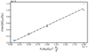 |
Fig. 23. Maximum contrast of differential rotation inside the DZ as a function of Pr(N0/Ω0)2Rec. The different symbols circle, square, hexagon and triangle respectively correspond to the simulations performed at Rec = 10−1, 5 × 10⁻¹, 1, and 2. Runs carried out at Lu = 5 × 10⁴ are presented in light blue, and those at Lu = 105, in blue. The other parameters are Pr(N0/Ω0)2 = 10−1, E = 10−5, Pm = 102, and ρi/ρ0 = 20.85 (runs D21–D24 and D27–D30 of Table 1). |
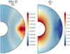 |
Fig. 24. Meridional cuts of the normalised differential rotation δΩ/Ω0 (left panel) and of the normalised norm of the poloidal field ∥Bp∥/B0(right panel). In black are also plotted the poloidal field lines to highlight the DZ. The parameters are Rec = 2, Lu = 5 × 10⁴, Pr(N0/Ω0)2 = 10−1, E = 10−5, Pm = 102, and ρi/ρ0 = 20.85 (run D38 of Table 1). |
7.4.2. Meridional circulation and differential rotation not confined to a dead zone
Simulations carried out at a smaller Pr(N0/Ω0)2 parameter (runs D32-D39 of Table 1) or at higher Rec (runs D38, Q14, Q16 and Q17 of Table 1), that is at higher values of τAp/τED and τAp/τc, exhibit different features. In the former case (smaller Pr(N0/Ω0)2), the differential rotation is no longer confined to the DZ as an AM redistribution by the Eddington–Sweet circulation occurs outside the DZ. In the second case (higher Rec), the amplitude of the meridional circulation is strong enough to warp the DZ and expel the magnetic flux there. These two phenomena are now discussed.
The left panel of Fig. 25 displays a meridional cut of the quasi-steady differential rotation (in colour) obtained for Rec = 1, Lu = 5 × 10⁴, and Pr(N0/Ω0)2 = 10−2 (run D36 of Table 1), on which are represented the vector lines of the total meridional velocity field as arrows and the poloidal field lines (in black). Compared to the simulation shown in Fig. 21, the ratio τAp/τED has been increased by a factor 20 (from 10−2 to 2 × 10⁻¹). Actually, if local values of this ratio are considered, a value of order 1 can be reached, in particular in the vicinity of the DZ. This is shown in the right panel of Fig. 25 that displays the distribution of the ratio of the Eddington–Sweet time to the local Alfvén time. In this regime, the differential rotation and the meridional circulation have spread out away from the DZ while the poloidal field lines, and thus the DZ, have not been affected by the circulation flow.
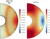 |
Fig. 25. Meridional cut of the normalised differential rotation δΩ/Ω0 (left panel) and 2D map comparing the Eddington–Sweet time to the Alfvén time (right panel). This one is locally estimated such as |
As presented in Fig. 26, another regime is encountered at sufficiently high Rec. The left panel of this figure displays the differential rotation in colour with the streamlines of the meridional circulation in black. The right panel shows, in colour, the norm of the poloidal field with the poloidal field lines in black. We observe that this meridional circulation significantly warps the DZ, thus leading to a reconfiguration of the magnetic field and the differential rotation. Compared to the simulation shown in the top panel of Fig. 21, the ratio τAp/τc has been increased by a factor of 6 (from 10−3 to 6 × 10⁻³). This is apparently sufficient for the Lorentz force not to be able to confine the circulation in the DZ. The magnetic field is then advected and partly dissipated in the vicinity of the original DZ. The dissipation process is reminiscent of the phenomenon of magnetic flux expulsion studied by Weiss (1966), whereby an eddy advects the magnetic field to such small scales that magnetic diffusion is efficient. We indeed observe that the magnetic flux ends up being expelled from the regions where the meridional circulation exists, and the poloidal field is found concentrated in free layers separating the quasi-solid rotation region from the one in differential rotation.
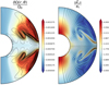 |
Fig. 26. Structure of the flow and of the magnetic field after ∼ 2τED. Left panel: coloured contours of the differential rotation normalised to the top value and streamlines (in black) of the meridional flow. Right panel: norm of the poloidal field normalised to its initial value at the pole of the outer sphere in colour with the poloidal field lines in black. The parameters are E = 10−5, Pr(N0/Ω0)2 = 10−1, ρi/ρ0 = 20.85, Pm = 102, Rec = 3 and Lu = 5 × 10⁴ (run Q16 of Table 1). |
8. Summary and conclusions
In this work, we investigated the dynamics of a contracting radiative spherical layer embedded in a large-scale magnetic field. The aim was to determine the differential rotation that results from the combined effects of contraction and magnetic fields. The contraction was modelled through an imposed radial velocity field Vf and the gas dynamics was modelled using either the Boussinesq or the anelastic approximations. The parametric study was guided by the results obtained without magnetic field (Gouhier et al. 2021) highlighting two hydrodynamical regimes, namely the viscous regime in the strongly stratified cases and the Eddington–Sweet regime in the weakly stratified cases.
We find that the contracting layer first evolves towards a quasi-steady configuration characterised by two magnetically decoupled regions. In the first region, all the poloidal field lines connect to the outer sphere. The rotation is quasi-uniform in this region because the contraction only allows very small deviations from Ferraro’s isorotation law along the field lines and the outer sphere rotates uniformly. The second region, called the DZ, is decoupled from the first one as the poloidal field lines loop-back on themselves or connect to the inner sphere. In addition, the poloidal field amplitude vanishes at some point within the DZ. A significant level of differential rotation can be produced in these DZs, the inward AM transport by the contraction being balanced either by a viscous transport or by an Eddington–Sweet circulation. The exact amplitude of the differential rotation also depends on the size, the shape and the location of the DZ.
In a second step, after a time of the order of the contraction time, the shear built in the DZ can trigger a powerful axisymmetric instability that profoundly modifies the subsequent evolution of the flow. Indeed, for an initial quadrupolar field in the viscous regime, we observe that if the field strength is low enough, an MRI-type instability grows and produces a multi-cellular meridional circulation organised at small scales in the radial direction. This flow advects and eventually enables to efficiently dissipate the magnetic energy. The new field configuration is strongly modified, and the differential rotation which is no longer constrained to the DZ spreads to most of the spherical layer while its amplitude increases. This instability has not been observed for the quadrupolar field in the Eddington–Sweet regime because numerical limitations did not allow us to reach significant levels of differential rotation. However, we anticipate that for realistic contraction Reynolds numbers and Lundquist numbers, the differential rotation in the DZ of the quadrupolar field will also trigger an instability in the Eddington–Sweet regime. By contrast, the dipolar field configuration does not lead to an instability. Indeed, in this case, the DZ is symmetric with respect to the equator and the contraction produces maximum rotation rates along the equator. The latitudinal differential rotation thus increases away from the rotation axis which implies stability with respect to the MRI. We note that the same configuration in an expanding layer would lead to minimum rotation rates along the equator and thus to differential rotations potentially unstable to MRI.
If we intent to extrapolate to a more complex geometry of the initial poloidal field, the dipolar topology with a single equatorially symmetric DZ appears exceptional. Thus, we expect that generically negative latitudinal gradients of the rotation rate, potentially unstable to the MRI, are present in DZs. Rather than the topology of the poloidal field, what can prevent the MRI to develop is its intensity. Indeed, according to Balbus & Hawley (1998), the magnetic tension stabilises the flow if the perturbation length scales λr are smaller than  . Applying this criteria to the degenerate core of a typical subgiant of 1.1 M⊙ and 2 R⊙, we find that, assuming a 𝒪(1) shear |q|, a rotation rate Ω = 3.1 × 10⁻⁶ rad s−1 and a mean core density
  kg m−3, fields higher than 3 × 10⁵ G will stabilise all the perturbations smaller than the degenerate core size of 0.06 R⊙. In practice, the radial wavelength of the unstable modes is constrained by the stable stratification rather than by the core size and thus even lower field intensities will be stabilising. For example, in our simulations λr is ∼44 times smaller than the outer radius of the spherical layer. The critical field in our numerical simulations is reached for a Lorentz number
  equal to ∼10−2. For the subgiant core rotation and density given above, this corresponds to a ∼104 G critical field strength. As Pr(N0/Ω0)2 and Pm of the simulations are not too far from realistic values in subgiant cores, and the shear should remain limited to 𝒪(1) even for more realistic contraction Reynolds numbers, this critical field extrapolated from the simulations might be of the right order of magnitude. To be more precise, a closer look at the MRI driven by a negative rotation latitudinal gradient in a radiative zone will be necessary.
Our numerical study thus points towards the following scenario: during a first period of the order of the contraction timescale, a contracting radiative layer embedded in a large-scale poloidal field tends to rotate uniformly, except in localised DZs where the contraction induces a significant differential rotation. If the field is weak enough and not purely dipolar, the development of a powerful axisymmetric MRI reconfigures the field and diminishes its intensity. The magnetic coupling then becomes inefficient in the major part of the radiative layer and the contraction can force the differential rotation there.
Such a scenario could potentially explain the evolution of the rotation of the subgiants between the end of the MS and the tip of the RGB. As mentioned in the introduction, the asteroseismic data can be reproduced by assuming a uniform rotation during a first period after the end of the MS followed by a second period where the contraction is left free to enforce differential rotation (Spada et al. 2016). This is consistent with the two young subgiants in near solid-body found by Deheuvels et al. (2020). At their age, the post-MS contraction should have increased their core rotation by a factor of four which means that the period of uniform rotation should last at least a contraction timescale. This timescale is compatible with our scenario.
Our simulations are nevertheless far to describe the full complexity of a magnetic and contracting subgiant. In particular, an expanding layer and boundary conditions mimicking the effect of a convective envelope should be added. The role of non-axisymmetric instabilities should also be considered, especially in the magnetic configuration that results from the axisymmetric instability. Non-axisymmetric MRI or Tayler instability might indeed be present and take part to the AM transport particularly along the giant branch as already invoked (Cantiello et al. 2014; Fuller et al. 2019).
As far as intermediate-mass stars are concerned, the occurrence of a powerful contraction-driven instability could help explain the dichotomy between Ap/Bp and Vega-like magnetisms. Indeed, strong Ap/Bp-like magnetic fields are expected to survive the instability during the PMS while below a certain field intensity, the axisymmetric MRI would change the pre-existing large-scale field into a small-scale field of smaller amplitude, thus leading to Vega-like magnetism. This is in line with the scenario proposed by Aurière et al. (2007), except that the instability invoked in this paper was a non-axisymmetric instability produced during the initial winding-up of the poloidal field by the differential rotation. Numerical investigations of this process confirmed the presence of such instabilities but not their ability to profoundly modify the pre-existing poloidal field (Jouve et al. 2015, 2020). By contrast, the axisymmetric MRI found in the present paper has a very strong impact on the initial poloidal field, destroying its large-scale structure and even diminishing its amplitude. To test this scenario, the threshold field strength that separates MRI stable and from MRI unstable configurations is crucial because it should be compatible with the observed 300 G lower bound of Ap/Bp surface magnetic fields. Again, this calls for further numerical and theoretical investigations of the critical field of the MRI driven by rotation latitudinal gradients in radiative zones.
Part of the above discussion is based on extrapolations of our numerical results to stellar conditions. Our simulations are indeed a simplified version of a contracting star. Among the simplifications, the ratio between the contraction time and the rotation time is larger in stars than in our simulations (τc/τΩ ∼ 3.4 × 10⁸ − 1.1 × 10¹¹ in stars while this ratio is comprised between 103 and 5 × 10⁵ in our simulations). However, the physical model derived from our simulation does not depend critically on this ratio. Indeed, by running our simulations for 5 − 6 contraction times, we observed that, after a contraction time, a powerful axisymmetric MHD instability develops. This leads to a complete reconfiguration of the initial magnetic field and to the subsequent development of differential rotation in most part of the spherical shell. This process should not be affected by increasing the ratio τc/τΩ to stellar values. In the same spirit, the ratio τΩ/τν, the Ekman number, is much lower in stars than in numerical simulations. But as shown in Gouhier et al. (2021), the hydrodynamical AM transport is not affected when this ratio is decreased by various orders of magnitude. Thus, despite the simplifications inherent to numerical simulations, the physical model derived from these simulations seems robust enough to apply to stars, especially in the viscous regime where the MRI has been observed. A question that remains to be addressed in future works concerns the occurrence of the MRI in more realistic Eddington–Sweet regimes which will require to explore the strongly non-linear regime corresponding to very large ratio τc/τν.
Acknowledgments
The authors acknowledge the developers of MagIC (https://github.com/magic-sph/magic) for the open-source code thanks to which the simulations were performed. This work was granted access to the HPC resources of CALMIP supercomputing center under the allocation P1118. L.J. acknowledges funding by the Institut Universitaire de France. The authors wish to thank Sébastien Deheuvels for very fruitful discussions.
References
- Acevedo-Arreguin, L., Garaud, P., & Wood, T. S. 2013, MNRAS, 434, 720 [NASA ADS] [CrossRef] [Google Scholar]
- Acheson, D., & Hide, R. 1973, Rep. Prog. Phys., 36, 159 [NASA ADS] [CrossRef] [Google Scholar]
- Alecian, E., Wade, G., Catala, C., et al. 2013, MNRAS, 429, 1001 [Google Scholar]
- Augustson, K. C., Brun, A. S., & Toomre, J. 2016, ApJ, 829, 92 [Google Scholar]
- Aurière, M., Wade, G., Silvester, J., et al. 2007, A&A, 475, 1053 [NASA ADS] [CrossRef] [EDP Sciences] [Google Scholar]
- Balbus, S. A., & Hawley, J. F. 1991, ApJ, 376, 214 [Google Scholar]
- Balbus, S. A., & Hawley, J. F. 1994, MNRAS, 266, 769 [NASA ADS] [Google Scholar]
- Balbus, S. A., & Hawley, J. F. 1998, Rev. Mod. Phys., 70, 1 [Google Scholar]
- Blazère, A., Petit, P., Lignières, F., et al. 2016, A&A, 586, A97 [NASA ADS] [CrossRef] [EDP Sciences] [Google Scholar]
- Braginsky, S. I., & Roberts, P. H. 1995, Geophys. Astrophys. Fluid Dyn., 79, 1 [Google Scholar]
- Braithwaite, J., & Spruit, H. C. 2004, Nature, 431, 819 [Google Scholar]
- Braithwaite, J., & Spruit, H. C. 2017, Roy. Soc. Open Sci., 4, 160271 [NASA ADS] [CrossRef] [Google Scholar]
- Brun, A. S., Browning, M. K., & Toomre, J. 2005, ApJ, 629, 461 [Google Scholar]
- Bugnet, L., Prat, V., Mathis, S., et al. 2021, A&A, 650, A53 [NASA ADS] [CrossRef] [EDP Sciences] [Google Scholar]
- Cally, P. 1991, J. Plasma Phys., 45, 453 [NASA ADS] [CrossRef] [Google Scholar]
- Cantiello, M., & Braithwaite, J. 2011, A&A, 534, A140 [NASA ADS] [CrossRef] [EDP Sciences] [Google Scholar]
- Cantiello, M., Mankovich, C., Bildsten, L., Christensen-Dalsgaard, J., & Paxton, B. 2014, ApJ, 788, 93 [Google Scholar]
- Cantiello, M., Fuller, J., & Bildsten, L. 2016, ApJ, 824, 14 [NASA ADS] [CrossRef] [Google Scholar]
- Ceillier, T., Eggenberger, P., García, R., & Mathis, S. 2013, A&A, 555, A54 [NASA ADS] [CrossRef] [EDP Sciences] [Google Scholar]
- Charbonneau, P., & MacGregor, K. 1993, ApJ, 417, 762 [NASA ADS] [CrossRef] [Google Scholar]
- Clune, T. C., Elliott, J., Miesch, M., Toomre, J., & Glatzmaier, G. A. 1999, Parallel Comput., 25, 361 [Google Scholar]
- Deheuvels, S., Doğan, G., Goupil, M., et al. 2014, A&A, 564, A27 [NASA ADS] [CrossRef] [EDP Sciences] [Google Scholar]
- Deheuvels, S., Ballot, J., Eggenberger, P., et al. 2020, A&A, 641, A117 [EDP Sciences] [Google Scholar]
- Donati, J.-F., & Landstreet, J. 2009, ARA&A, 47, 333 [NASA ADS] [CrossRef] [Google Scholar]
- Dormy, E., Cardin, P., & Jault, D. 1998, Earth Planet. Sci. Lett., 160, 15 [CrossRef] [Google Scholar]
- Eggenberger, P., Montalbán, J., & Miglio, A. 2012, A&A, 544, L4 [NASA ADS] [CrossRef] [EDP Sciences] [Google Scholar]
- Eggenberger, P., Deheuvels, S., Miglio, A., et al. 2019, A&A, 621, A66 [NASA ADS] [CrossRef] [EDP Sciences] [Google Scholar]
- Ferraro, V. C. 1937, MNRAS, 97, 458 [CrossRef] [Google Scholar]
- Fuller, J., Cantiello, M., Stello, D., García, R. A., & Bildsten, L. 2015, Science, 350, 423 [NASA ADS] [CrossRef] [Google Scholar]
- Fuller, J., Piro, A. L., & Jermyn, A. S. 2019, MNRAS, 485, 3661 [NASA ADS] [Google Scholar]
- Gallet, F., & Bouvier, J. 2013, A&A, 556, A36 [NASA ADS] [CrossRef] [EDP Sciences] [Google Scholar]
- Garaud, P. 2002, MNRAS, 335, 707 [CrossRef] [Google Scholar]
- Garaud, P., & Acevedo-Arreguin, L. 2009, ApJ, 704, 1 [NASA ADS] [CrossRef] [Google Scholar]
- Garaud, P., & Brummell, N. 2008, ApJ, 674, 498 [NASA ADS] [CrossRef] [Google Scholar]
- Garaud, P., & Garaud, J.-D. 2008, MNRAS, 391, 1239 [NASA ADS] [CrossRef] [Google Scholar]
- Garaud, P., Medrano, M., Brown, J., Mankovich, C., & Moore, K. 2015, ApJ, 808, 89 [Google Scholar]
- Gastine, T., & Wicht, J. 2012, Icarus, 219, 428 [Google Scholar]
- Gouhier, B., Lignières, F., & Jouve, L. 2021, A&A, 648, A109 [EDP Sciences] [Google Scholar]
- Heyvaerts, J., & Priest, E. 1983, A&A, 117, 220 [NASA ADS] [Google Scholar]
- Hollerbach, R., & Rüdiger, G. 2005, Phys. Rev. Lett., 95, 124501 [NASA ADS] [CrossRef] [Google Scholar]
- Jones, C., Boronski, P., Brun, A., et al. 2011, Icarus, 216, 120 [Google Scholar]
- Jouve, L., Gastine, T., & Lignières, F. 2015, A&A, 575, A106 [NASA ADS] [CrossRef] [EDP Sciences] [Google Scholar]
- Jouve, L., Lignières, F., & Gaurat, M. 2020, A&A, 641, A13 [EDP Sciences] [Google Scholar]
- Kirillov, O. N., Stefani, F., & Fukumoto, Y. 2014, J. Fluid Mech., 760, 591 [NASA ADS] [CrossRef] [Google Scholar]
- Knobloch, E. 1992, MNRAS, 255, 25P [CrossRef] [Google Scholar]
- Lantz, S. R. 1992, PhD Thesis, Cornell University, USA [Google Scholar]
- Lignières, F., Califano, F., & Mangeney, A. 1999, A&A, 349, 1027 [NASA ADS] [Google Scholar]
- Lignières, F., Petit, P., Böhm, T., & Aurière, M. 2009, A&A, 500, L41 [CrossRef] [EDP Sciences] [Google Scholar]
- Lignières, F., Petit, P., Aurière, M., Wade, G. A., & Böhm, T. 2014, Proc. Int. Astron. Union, 9, 338 [Google Scholar]
- Maeder, A. 2008, Physics, Formation and Evolution of Rotating Stars (Berlin: Springer Science& Business Media) [Google Scholar]
- Marques, J., Goupil, M., Lebreton, Y., et al. 2013, A&A, 549, A74 [NASA ADS] [CrossRef] [EDP Sciences] [Google Scholar]
- Menou, K., Balbus, S. A., & Spruit, H. C. 2004, ApJ, 607, 564 [NASA ADS] [CrossRef] [Google Scholar]
- Mestel, L., & Weiss, N. 1987, MNRAS, 226, 123 [CrossRef] [Google Scholar]
- Mosser, B., Elsworth, Y., Hekker, S., et al. 2012, A&A, 537, A30 [NASA ADS] [CrossRef] [EDP Sciences] [Google Scholar]
- Mosser, B., Belkacem, K., Pinçon, C., et al. 2017, A&A, 598, A62 [NASA ADS] [CrossRef] [EDP Sciences] [Google Scholar]
- Oglethorpe, R., & Garaud, P. 2013, ApJ, 778, 166 [NASA ADS] [CrossRef] [Google Scholar]
- Petit, P., Lignières, F., Wade, G., et al. 2010, A&A, 523, A41 [NASA ADS] [CrossRef] [EDP Sciences] [Google Scholar]
- Petit, P., Lignières, F., Aurière, M., et al. 2011, A&A, 532, L13 [NASA ADS] [CrossRef] [EDP Sciences] [Google Scholar]
- Petitdemange, L., Dormy, E., & Balbus, S. 2013, Phys. Earth Planet. Inter., 223, 21 [CrossRef] [Google Scholar]
- Roberts, P. 1967, Proc. R. Soc. London, Ser. A. Math. Phys. Sci., 300, 94 [Google Scholar]
- Rüdiger, G., Gellert, M., Spada, F., & Tereshin, I. 2015, A&A, 573, A80 [NASA ADS] [CrossRef] [EDP Sciences] [Google Scholar]
- Rüdiger, G., Schultz, M., & Kitchatinov, L. 2016, MNRAS, 456, 3004 [CrossRef] [Google Scholar]
- Rüdiger, G., Gellert, M., Hollerbach, R., Schultz, M., & Stefani, F. 2018, Phys. Rep., 741, 1 [CrossRef] [Google Scholar]
- Shercliff, J. 1956, J. Fluid Mech., 1, 644 [NASA ADS] [CrossRef] [Google Scholar]
- Spada, F., Gellert, M., Arlt, R., & Deheuvels, S. 2016, A&A, 589, A23 [NASA ADS] [CrossRef] [EDP Sciences] [Google Scholar]
- Spruit, H. 1999, A&A, 349, 189 [NASA ADS] [Google Scholar]
- Spruit, H. 2002, A&A, 381, 923 [CrossRef] [EDP Sciences] [Google Scholar]
- Stefani, F., Gundrum, T., Gerbeth, G., et al. 2006, Phys. Rev. Lett., 97, 184502 [NASA ADS] [CrossRef] [Google Scholar]
- Stello, D., Cantiello, M., Fuller, J., García, R. A., & Huber, D. 2016a, PASA, 33 [Google Scholar]
- Stello, D., Cantiello, M., Fuller, J., et al. 2016b, Nature, 529, 364 [Google Scholar]
- Wade, G. A., Drouin, D., Bagnulo, S., et al. 2005, A&A, 442, L31 [NASA ADS] [CrossRef] [EDP Sciences] [Google Scholar]
- Weiss, N. O. 1966, Proc. R. Soc. London, Ser. A. Math. Phys. Sci., 293, 310 [Google Scholar]
- Wicht, J. 2002, Phys. Earth and Planet. Inter., 132, 281 [CrossRef] [Google Scholar]
- Wood, T. S., & Brummell, N. H. 2012, ApJ, 755, 99 [NASA ADS] [CrossRef] [Google Scholar]
- Wood, T. S., & Brummell, N. H. 2018, ApJ, 853, 97 [NASA ADS] [CrossRef] [Google Scholar]
- Zahn, J.-P. 1992, A&A, 265, 115 [NASA ADS] [Google Scholar]
Appendix A: Electrical-current function
In this appendix, we determine the stream function that is constant along the streamlines of the poloidal component of the current density jp. The toroidal component of the magnetic field is related to jp through

As the divergence of the curl is zero and the problem is axisymmetric, we can define a vector potential χ as
from which we define the electrical-current stream function 𝒥p = r sin θχ:
We thus obtain a relationship between the toroidal field and the electrical-current stream function:

By integrating the first equation we have
and substituting in the second equation we deduce
As the electrical-current stream function is zero at the poles, we conclude that cte = 0 hence:
Appendix B: Hartmann boundary layer equations
In the present appendix, the Hartmman boundary layer equations are derived with the aim of relating the jump of the toroidal field across the layer with the differential rotation jump. The Hartmann layer occurs at the electrically insulating outer boundary where the azimuthal velocity is fixed and a magnetic field perpendicular to the flow is present. When the contraction term is removed from the induction equation, the governing equations for the azimuthal flow and the toroidal field component in the steady linear limit read:
![$$ \begin{aligned} \begin{array}{lll} 2 \Omega _0 \left(U_s - \sin {\theta } \displaystyle \frac{V_0 r_0^2}{r^2}\right) = \displaystyle \frac{1}{\mu _0 \rho _0} \left[\displaystyle \frac{B_{\theta }}{r} \displaystyle \frac{\partial B_{\phi }}{\partial \theta } + \displaystyle \frac{\cot {\theta }}{r} B_{\theta } B_{\phi } + B_r \displaystyle \frac{\partial B_{\phi }}{\partial r} + \displaystyle \frac{B_r B_{\phi }}{r} \right]+ \\ \\ \nu \left[\displaystyle \frac{\partial ^2 U_{\phi }}{\partial r^2} + \displaystyle \frac{2}{r} \displaystyle \frac{\partial U_{\phi }}{\partial r} + \displaystyle \frac{1}{r^2} \displaystyle \frac{\partial ^2 U_{\phi }}{\partial \theta ^2} + \displaystyle \frac{\cot {\theta }}{r^2} \displaystyle \frac{\partial U_{\phi }}{\partial \theta } - \displaystyle \frac{U_{\phi }}{r^2 \sin ^2 \theta } \right], \end{array} \end{aligned} $$](/articles/aa/full_html/2022/05/aa41613-21/aa41613-21-eq108.gif)
![$$ \begin{aligned} \begin{array}{lll} U_r \displaystyle \frac{\partial B_{\phi }}{\partial r} + \displaystyle \frac{U_{\theta }}{r} \displaystyle \frac{\partial B_{\phi }}{\partial \theta } - B_r \displaystyle \frac{\partial U_{\phi }}{\partial r} - \displaystyle \frac{B_{\theta }}{r} \displaystyle \frac{\partial U_{\phi }}{\partial \theta } + U_{\phi } \left(\displaystyle \frac{B_r}{r} + \displaystyle \frac{\cot {\theta } B_{\theta }}{r} \right) - B_{\phi } \left(\displaystyle \frac{U_r}{r} + \displaystyle \frac{\cot {\theta } U_{\theta }}{r} \right) = \\ \\ \eta \left[\displaystyle \frac{\partial ^2 B_{\phi }}{\partial r^2} + \displaystyle \frac{2}{r} \displaystyle \frac{\partial B_{\phi }}{\partial r} + \displaystyle \frac{1}{r^2} \displaystyle \frac{\partial ^2 B_{\phi }}{\partial \theta ^2} + \displaystyle \frac{\cot {\theta }}{r^2} \displaystyle \frac{\partial B_{\phi }}{\partial \theta } - \displaystyle \frac{B_{\phi }}{r^2 \sin ^2 \theta } \right]. \end{array} \end{aligned} $$](/articles/aa/full_html/2022/05/aa41613-21/aa41613-21-eq109.gif)
Since in our simulations the Elsasser number  is ≫1, the Coriolis term becomes negligible with respect to the Lorentz force (Acheson & Hide 1973), then, assuming Ur ≪ Uϕ and conserving the highest radial derivatives in each term, we get the Hartmann boundary layer equations (see also reviews by Roberts (1967), Acheson & Hide (1973), Dormy et al. (1998)):
where the index H denotes a boundary layer flow. As Br(r0, θ) = − B0 cos θ (see Eq. (22)), then after introducing the stretched coordinate  , Sys. (B.3) is rewritten as:

By deriving the second of these two equations,  can be eliminated to yield:
whose the solution is

From the evanescent condition when ξ → ∞, C1 = C3 = 0, and from the vacuum condition at the outer sphere  ,
,  , hence:
This time, the index I stands for interior flow. We now integrate the second equation of Sys. (B.4):
Again, from the evanescent equation when ξ → ∞, we readily get C4 = 0. Then, as  at the outer sphere, we obtain the following relationship between the interior flows:
and,
Thus, using the estimate Eq. (36), we deduce from Eq. (B.9) the order of magnitude of the jump on the differential rotation across the Hartmann layer

In Fig. B.1, we plotted the normalised toroidal field Bϕ/B0 (left panel) and the normalised differential rotation δΩ/Ω0 (right panel) as a function of the stretched coordinate ξ at the particular location θ = π/4. This was done for runs obtained at various Lu ranging from 5 ⋅ 103 to 5 ⋅ 104, both for Rec = 1 and 5 (runs D3 to D7 of Table 1). These quantities have been rescaled with their characteristic amplitude as given by Eqs. (36) and (B.11). We can observe that the different curves overlap and are of 𝒪(1) after rescaling. This enables us to conclude that the 𝒪(r0μ0ρ0V0Ω0/B0) jump on the toroidal magnetic field at the outer sphere induces a  jump on the azimuthal component of the velocity field across the Hartmann layer or equivalently, a
  jump on the normalised differential rotation. As a result, the quasi-solid rotation region is in differential rotation with the outer sphere and the characteristic amplitude of this differential rotation is given by Eq. (B.11).
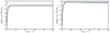 |
Fig. B.1. Toroidal field normalised to B0 (left panel) and differential rotation normalised to Ω0 (right panel), respectively rescaled by |


Appendix C: Approximate solutions of differential rotation in the dead zone
C.1. Case 1 - No effect of the contraction on the field lines
This appendix is intended to solve in the DZ the viscous balance Eq. (35), whose dimensionless form reads
To do so, the DZ is assimilated to a conical domain as sketched in Fig. C.1. This domain, denoted 𝒟, is such that:

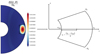 |
Fig. C.1. Sketch of the conical domain chosen to represent the DZ when the field lines are not advected by the contraction. The displayed meridional cut of the normalised rotation rate is the same as in the first panel of Fig. 3. The conical domain, delimited by thick black lines on the meridional cut, is defined by r ∈ [riDZ;r0] and θ ∈ [−θ0;θ0], with riDZ = 0.77r0, θ0 ≈ π/14, and −θ0 ≈ −π/14 or equivalently, in terms of colatitude, θ ∈ [3π/7;4π/7]. |
where riDZ = 0.77r0 and the latitude θ0 is ≈π/14. In addition, we assume that the term  is negligible as compared to the others. This assumption has been verified a posteriori. Thus, Eq. (C.1) is rewritten as follows:
Outside the domain 𝒟, the flow is assumed to be in solid rotation and symmetrical with respect to the equatorial plane so that we adopt the following homogeneous boundary conditions:
The method for solving Eq. (C.3) was excerpted from a lecture of the Ira A. Fulton College of Engineering and Technology at Brigham Young University 2. The broad lines are now given. We first build a set of basis functions that will be used to express the solution. These are obtained by looking for separable solutions of the eigenvalue problem
satisfying the boundary conditions Eq. (C.4). We finally determine a general solution using the orthogonality properties of the basis functions.
Separable solutions,  , of Eq. (C.5) must verify:

with the boundary conditions

The problem thus reduces to the solving the two following sub-eigenvalue problems:

The differential equation in θ is a classical Sturm-Liouville problem while the differential equation in r is known as the Euler’s problem. We first deal with the Sturm-Liouville problem.
In order to avoid unphysical solutions, the eigenvalues must be strictly negative. The solution then reads

Its latitudinal derivative is readily

From the condition of symmetry,  and
and  . Besides,
  . Since we are looking for a non-trivial solution (i.e.
  ) we obtain
thus concluding that
are the sought eigenvalues and are associated with the eigenfunctions
We are now going to solve the Euler’s problem. Here the eigenvalues must be < − 9/4 to avoid unphysical solutions. In that case, the solution reads:

which can be rewritten as

From the condition  we have
  , and
, and
The second boundary condition leads to
Excluding the non-trivial solution  we obtain
The sought eigenvalues are thus

and are associated with the eigenfunctions
The general solution δΩ(r, θ) is now expanded over the basis of the eigenfunctions satisfying the boundary conditions Eq. (C.7):

Thus, this solution verifies the boundary conditions Eq. (C.4). We now need to find the Ank coefficients. These are determined using the orthogonality properties of the eigenfunctions. After determining the different partial derivatives of the function δΩ(r, θ) and after substituting their expressions in Eq. (C.3), we obtain the following relationship:
![$$ \begin{aligned} \sum _{n=1}^{\infty } \sum _{k=1}^{\infty } \displaystyle \frac{\tilde{A}_{nk}}{\sqrt{\tilde{r}}} \left[- \left(\displaystyle \frac{3}{2}\right)^2 - \left(\displaystyle \frac{n\pi }{\ln \left(\tilde{r}_{i_{\mathrm{DZ} }}\right)}\right)^2 - \left( \displaystyle \frac{\left(2k - 1\right) \pi }{2 \theta _0} \right)^2 \right]\sin {\left(\left(\displaystyle \frac{n \pi }{\ln {\left(\tilde{r}_{i_{\mathrm{DZ} }}\right)}}\right)\ln {\left(\tilde{r}\right)} \right)} \cos {\left(\left( \displaystyle \frac{\left(2k - 1\right) \pi }{2 \theta _0} \right) \theta \right)} = \displaystyle \frac{-2}{E} . \end{aligned} $$](/articles/aa/full_html/2022/05/aa41613-21/aa41613-21-eq159.gif)
As
![$$ \begin{aligned} \tilde{\lambda }_{nk} = \left[\underbrace{-\left(\displaystyle \frac{3}{2}\right)^2 - \left(\displaystyle \frac{n\pi }{\ln \left(\tilde{r}_{i_{\mathrm{DZ} }}\right)}\right)^2}_{\left|\tilde{\mu }_n\right|} \underbrace{- \left( \displaystyle \frac{\left(2k - 1\right) \pi }{2 \theta _0} \right)^2}_{\left|\tilde{\nu }_k \right|} \right]\quad \mathrm{with} \quad n, k \in \mathbb{Z} , \end{aligned} $$](/articles/aa/full_html/2022/05/aa41613-21/aa41613-21-eq160.gif)
Eq. (C.22) is rewritten as follows
Multiplying each members of this relationship by  , then integrating over the domain 𝒟 the resulting relationship, we obtain the coefficients Ank:
![$$ \begin{aligned} \tilde{A}_{nk} = \left( \displaystyle \frac{4 \left(n\pi \right)^2 + \left(\ln {\left(\tilde{r}_{i_{\mathrm{DZ} }}\right)} \right)^2}{E \tilde{\lambda }_{nk} \left(\tilde{r}_{i_{\mathrm{DZ} }}-1\right) \left(n\pi \right)^2 \theta _0 } \right) \left( \displaystyle \frac{-4 \theta _0}{\left(2k-1\right)\pi } \left(-1 \right)^{k} \right) \left( \displaystyle \frac{4 n \pi \ln {\left(\tilde{r}_{i_{\mathrm{DZ} }}\right)}}{4 \left(n\pi \right)^2 + 9 \left( \ln {\left(\tilde{r}_{i_{\mathrm{DZ} }}\right)} \right)^2} \left[\left(-1\right)^n \tilde{r}_{i_{\mathrm{DZ} }}^{3/2} - 1 \right]\right) \quad \mathrm{with} \quad n, k \in \mathbb{Z} , \end{aligned} $$](/articles/aa/full_html/2022/05/aa41613-21/aa41613-21-eq163.gif)
and the final solution, which reads under dimensional form
![$$ \begin{aligned} \displaystyle \frac{\delta \Omega (r,\theta )}{\Omega _0}&= Re_c \sum _{n=1}^{\infty } \sum _{k=1}^{\infty } \left[ \left( \displaystyle \frac{\left(2n\pi \right)^2 + \left(\ln {\left(\displaystyle \frac{r_{i_{ \text{DZ}}}}{r_0}\right)} \right)^2}{\lambda _{nk} \left(\displaystyle \frac{r_{i_{\text{DZ}}}}{r_0}-1\right) \left(n\pi \right)^2 \theta _0 } \right) \left( \displaystyle \frac{-4 \theta _0}{\left(2k-1\right)\pi } \left(-1 \right)^{k} \right) \left( \displaystyle \frac{4 n \pi \ln {\left(\displaystyle \frac{r_{i_{ \text{DZ}}}}{r_0}\right)}}{\left(2n\pi \right)^2 + \left( 3\ln {\left(\displaystyle \frac{r_{i_{ \text{DZ}}}}{r_0}\right)} \right)^2} \left( \left(-1\right)^n \left(\displaystyle \frac{r_{i_{ \text{DZ}}}}{r_0}\right)^{3/2} - 1 \right) \right) \right.\nonumber \\& \left( \displaystyle \frac{r_0}{r} \right)^{3/2} \left.\sin {\left(\left(\displaystyle \frac{n \pi }{\ln {\left(\displaystyle \frac{r_{i_{ \text{DZ}}}}{r_0}\right)}}\right) \ln {\left(\displaystyle \frac{r}{r_0}\right)} \right)} \cos {\left(\left( \displaystyle \frac{\left(2k - 1\right) \pi }{2 \theta _0} \right) \theta \right)} \right] \normalsize \quad \mathrm{with} \quad n, k \in \mathbb{Z} . \end{aligned} $$](/articles/aa/full_html/2022/05/aa41613-21/aa41613-21-eq164.gif)
C.2. Case 2 - Advection of the field lines by the contraction
When the contraction term is introduced in the induction equation, the poloidal field lines are advected and the DZ connects to the inner sphere (see Fig. C.2). This modifies the boundary conditions Eq. (C.4) since at the inner sphere, the azimuthal component of the velocity field now satisfies a stress-free condition hence:
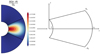 |
Fig. C.2. Sketch of the conical domain chosen to represent the DZ when the field lines are advected by the contraction. The displayed meridional cut of the normalised rotation rate is the same as in the third panel of Fig. 3. The conical domain, delimited by thick black lines on the meridional cut, is defined by r ∈ [ri;r0] and θ ∈ [−θ0;θ0], where θ0 ≈ 4π/23 and −θ0 ≈ −4π/23 or equivalently, in terms of colatitude, θ ∈ [15π/46;31π/46]. |
Thus, the solution of the Sturm-Liouville problem is unchanged and the sought eigenvalues are again Eq. (C.12) and are associated with the eigenfunctions Eq. (C.13). For the Euler’s problem, the eigenvalues must still be < 9/4 to avoid unphysical solutions. By taking Eq. (C.15), and after using the condition  , we have

By deriving this expression to apply the stress-free condition to it, we get the transcendental equation
After numerically solving this equation, we obtain the eigenvalues μn. The general solution δΩ(r, θ) of Eq. (C.3) is then expanded on the basis of the eigenfunctions satisfying the boundary conditions Eq. (C.27) on the domain 𝒟

As previously, after determining the different partial derivatives of the function δΩ(r, θ), and after substituting them in Eq. (C.3), we get:
![$$ \begin{aligned} \sum _{n=1}^{\infty } \sum _{k=1}^{\infty } \displaystyle \frac{\tilde{A}_{nk}}{\sqrt{\tilde{r}}} \left[\underbrace{\tilde{\mu }_n - \left( \displaystyle \frac{\left(2k - 1\right) \pi }{2 \theta _0} \right)^2}_{\tilde{\lambda }_{nk}} \right]\sin {\left( \displaystyle \frac{1}{2} \sqrt{\left|9 + 4 \tilde{\mu }_n \right|} \ln {\left(\tilde{r}\right)} \right)} \cos {\left(\left( \displaystyle \frac{\left(2k - 1\right) \pi }{2 \theta _0} \right) \theta \right)} = \displaystyle \frac{-2}{E} . \end{aligned} $$](/articles/aa/full_html/2022/05/aa41613-21/aa41613-21-eq170.gif)
Again, using the orthogonality properties enables us to determine the Ank coefficients
![$$ \begin{aligned} \begin{array}{lll} \tilde{A}_{nk} = \displaystyle \frac{\left[2 \sqrt{\left| 9 + 4 \tilde{\mu }_n \right|} \left(\tilde{r}_i^{3/2} \cos {\left(\displaystyle \frac{1}{2} \sqrt{\left| 9 + 4 \tilde{\mu }_n \right|} \ln {(\tilde{r}_i)} \right)} -1 \right) - 6 \tilde{r}_i^{3/2} \sin {\left(\displaystyle \frac{1}{2} \sqrt{\left| 9 + 4 \tilde{\mu }_n \right|} \ln {(\tilde{r}_i)}\right)} \right]}{\left[\left| 9 + 4 \tilde{\mu }_n \right| \left(1 - \tilde{r}_i\right) + \tilde{r}_i \left( \cos {\left(\sqrt{\left| 9 + 4 \tilde{\mu }_n \right|}\ln {(\tilde{r}_i)}\right)} + \sqrt{\left| 9 + 4 \tilde{\mu }_n \right|} \sin {\left(\sqrt{\left| 9 + 4 \tilde{\mu }_n \right|}\ln {(\tilde{r}_i)}\right)} -1 \right) \right]} \cdot \\ \\ \displaystyle \frac{16 \left(1 + \left| 9 + 4 \tilde{\mu }_n \right| \right) \left(-1\right)^k}{E \tilde{\lambda }_{nk} \left(2k-1\right) \left(9 + \left| 9 + 4 \tilde{\mu }_n \right|\right) \pi }, \end{array} \end{aligned} $$](/articles/aa/full_html/2022/05/aa41613-21/aa41613-21-eq171.gif)
and so the final solution which, under dimensional form, reads as follows:
![$$ \begin{aligned} \begin{array}{lll} \displaystyle \frac{\delta \Omega (r,\theta )}{\Omega _0} = Re_c \displaystyle \sum _{n=1}^{\infty } \displaystyle \sum _{k=1}^{\infty } \displaystyle \frac{\left[2 \sqrt{\left| 9 + 4 \mu _n \right|} \left(\left(\displaystyle \frac{r_i}{r_0}\right)^{3/2} \cos {\left(\displaystyle \frac{1}{2} \sqrt{\left| 9 + 4 \mu _n \right|} \ln {\left(\displaystyle \frac{r_i}{r_0}\right)} \right)} -1 \right) - 6 \left(\displaystyle \frac{r_i}{r_0}\right)^{3/2} \sin {\left(\displaystyle \frac{1}{2} \sqrt{\left| 9 + 4 \mu _n \right|} \ln {\left(\displaystyle \frac{r_i}{r_0}\right)}\right)} \right]}{\left[\left| 9 + 4 \mu _n \right| \left(1 - \displaystyle \frac{r_i}{r_0}\right) + \displaystyle \frac{r_i}{r_0} \left( \cos {\left(\sqrt{\left| 9 + 4 \mu _n \right|}\ln {\left(\displaystyle \frac{r_i}{r_0}\right)}\right)} + \sqrt{\left| 9 + 4 \mu _n \right|} \sin {\left(\sqrt{\left| 9 + 4 \mu _n \right|}\ln {\left(\displaystyle \frac{r_i}{r_0}\right)}\right)} - 1 \right) \right]} \\ \\ \displaystyle \frac{16 \left(1 + \left| 9 + 4 \mu _n \right|\right) \left(-1\right)^k}{\lambda _{nk} \left(2k-1\right) \left(9 + \left| 9 + 4 \mu _n \right|\right) \pi } \displaystyle \left(\frac{r_0}{r}\right)^{3/2} \sin {\left( \displaystyle \frac{1}{2} \sqrt{\left|9 + 4 \mu _n \right|} \ln {\left(\displaystyle \frac{r}{r_0}\right)} \right)} \cos {\left(\left( \displaystyle \frac{\left(2k - 1\right) \pi }{2 \theta _0} \right) \theta \right)} ,\end{array} \end{aligned} $$](/articles/aa/full_html/2022/05/aa41613-21/aa41613-21-eq172.gif)
where n, k ∈ ℤ.
All Tables
Parameters of the simulations performed at Pm = 102 in the viscous and Eddington–Sweet regimes.
Ratio between the growth rate σi = 1, 2, 3 of the instability and the product of the absolute value of the surface-averaged shear parameter |⟨q⟩| by the local rotation rate Ω.
All Figures
|
Fig. 1. Meridional cuts of the norm of the initial magnetic field (colour) for the dipole Eq. (22) (left), and the quadrupole Eq. (23) (right). The black lines show the poloidal field lines. |
| In the text | |
|
Fig. 2. Illustration of the unsteady phase. Left panel: meridional cut of the norm of the poloidal magnetic field. The black dots show the position of 5 control points located on different field lines. In the other two panels, the temporal evolution of these points is followed during 20τAp, both for the toroidal field Bϕc (middle panel) and the normalised differential rotation ΔΩc/Ω0 (right panel). The parameters are E = 10−4, Pr(N0/Ω0)2 = 104, Rec = 1, Lu = 5 × 10⁴, and Pm = 102 (run D5 of Table 1). |
| In the text | |
|
Fig. 3. Meridional cuts of the rotation rate normalised to the value at the outer sphere (first and third panels) and toroidal field (second and fourth panels), in the quasi-steady state. In black lines are also represented the poloidal field lines (first and third panels) and the streamlines associated with the electrical-current function defined in Appendix A (second and fourth panels). The dotted (solid) lines then correspond to an anticlockwise (clockwise) current circulation. In the first two panels, the contraction does not advect the poloidal field lines and the quasi-steady state is achieved after ∼0.04τc (i.e. ∼ 20τAp, see Fig. 2). In the last two panels such an advection is allowed and the quasi-steady configuration is reached after ∼1τc (i.e. after ∼100τAp for this simulation). For these two cases, the Lundquist numbers are respectively Lu = 5 × 10⁴ and Lu = 104 (runs D5 and D13). The other parameters are identical, namely Pr(N0/Ω0)2 = 104, E = 10−4, Rec = 1, and Pm = 102. |
| In the text | |
|
Fig. 4. 2D maps comparing the relative importance of different azimuthally projected quantities: the Lorentz force with the contraction (first two panels) and the viscous term with the contraction (last two panels). The runs where the contraction term has been removed from the induction equation are presented in the first and third panels. In the other two, the effect of the contraction on the magnetic field is taken into account. The parameters are the same to those of Fig. 3. |
| In the text | |
|
Fig. 5. Normalised rotation rate in the quasi-steady state. Top panel (5a): this is the third panel of Fig. 3 presented on a smaller rotation rate scale. As a result, the DZ is saturated in colour. Bottom panel (5b): enlargement of the black-delimited zone displayed in the top panel. In each panels, the poloidal field lines are also represented (black lines). For the sake of clarity, every other field line is plotted in red in the bottom panel. The parameters are the same as in Figs. 3 and 4. |
| In the text | |
|
Fig. 6. Toroidal field Bϕ normalised to the initial amplitude of the poloidal field B0, as a function of (Pm/Lu)2Rec/E and at the particular location θ = π/6 and r = 0.65r0. The different symbols correspond to the different runs D1–D7 of Table 1 (no contraction term in induction equation) namely, Rec = 10−1, Lu = 104 (circle); Rec = 10−1, Lu = 5 × 10⁴ (square); Rec = 1, Lu = 5 × 10³ (hexagon); Rec = 1, Lu = 104 (up triangle); Rec = 1, Lu = 5 × 10⁴ (pentagon); Rec = 5, Lu = 104 (down triangle) and Rec = 5, Lu = 5 × 10⁴ (diamond). The other parameters are fixed to E = 10−4, Pr(N0/Ω0)2 = 104, and Pm = 102. |
| In the text | |
|
Fig. 7. Normalised differential rotation between a point outside the DZ and the outer sphere, ΔΩ/Ω0 = (Ω(r = 0.65r0,θ=π/12)−Ω0)/Ω0, plotted as a function of |
| In the text | |
|
Fig. 8. Normalised differential rotation along a poloidal field line ΔΩpol/Ω0 as a function of (RecPm/Lu)2. This quantity is estimated between two sufficiently separated points along a field line for the runs D8 and, D10–D14 of Table 1. The correspondences between parameters and symbols are as follows: circle: Rec = 10−1, Lu = 104; triangle: Rec = 5 × 10⁻¹, Lu = 5 × 10³; diamond: Rec = 5 × 10⁻¹, Lu = 104; square: Rec = 1, Lu = 5 × 10³; pentagon: Rec = 1, Lu = 104; hexagon: Rec = 2, Lu = 104. The other parameters are E = 10−4, Pr(N0/Ω0)2 = 104, and Pm = 102. |
| In the text | |
|
Fig. 9. Temporal evolution of different quantities followed over a period of 300τAp: the toroidal field normalised to the initial amplitude of the poloidal field and rescaled by |
| In the text | |
|
Fig. 10. Equatorial differential rotation as a function of radius when the contraction term is removed from the induction equation. Numerical solutions (runs D1–D7) are plotted in colour at Rec = 10−1 (red), Rec = 1 (blue), and Rec = 5 (purple), for various Lundquist numbers ranging from 104 to 5 × 10⁴ (from the lightest to the darkest). For Rec = 1, an additional simulation is presented at Lu = 5 × 10³. The curves are rescaled by Rec then compared to the analytical solution Eq. (39) displayed in black dashed lines. The other parameters are E = 10−4, Pr(N0/Ω0)2 = 104, and Pm = 102. |
| In the text | |
|
Fig. 11. Same as Fig. 10 but for cases where contraction acts on the field lines. The simulations presented here are the runs D10–D14 of Table 1 performed at Rec = 5 × 10⁻¹ (green), Rec = 1 (blue), and Rec = 2 (purple). For all these cases Lu = 104, but for Rec = 5 × 10⁻¹ and 1, additional simulations are shown at Lu = 5 × 10³ in dash-dot lines. The analytical solution Eq. (40) is displayed in black dashed lines. |
| In the text | |
|
Fig. 12. Meridional cuts of the normalised rotation rate in two anelastic cases with ρi/ρ0 = 20.85. The poloidal field lines are represented in black lines. For these simulations the contraction term is included in the induction equation. In the first panel, Rec = 1 and Lu = 105 (run D18 of Table 1). In the second one, Rec = 5 and Lu = 5 × 10⁴ (run D20 of Table 1). The other parameters are Pr(N0/Ω0)2 = 104, E = 10−4, and Pm = 102. |
| In the text | |
|
Fig. 13. Same as Fig. 3, but for the initially quadrupolar magnetic field. In the first two panelsLu = 5 × 10⁴, while Lu = 104 in the last two. The other parameters are Rec = 1, E = 10−4, Pr(N0/Ω0)2 = 104, and Pm = 102 (runs Q2 and Q10 of Table 1). |
| In the text | |
|
Fig. 14. Maximum value of the normalised differential rotation max(ΔΩ/Ω0) as a function of the contraction timescale as defined in Eq. (12). The main evolution steps are highlighted by coloured dashed lines: the red dashed lines corresponds to the start of the exponential growth phase and orange, to the time at which the instability saturates, thus marking the beginning of the non-linear evolution. Then, blue marks the start of the post-instability evolution and finally, purple denotes the time at which the hydrodynamic steady state is reached. The parameters are Rec = 1, Lu = 104, E = 10−4, Pr(N0/Ω0)2 = 104, and Pm = 102 (run Q10 of Table 1, contraction term in induction equation). |
| In the text | |
|
Fig. 15. Axisymmetric instability in the viscous regime when the quadrupolar field given by Eq. (23) and illustrated in Fig. 1, is initially imposed. First two panels: snapshots of the latitudinal component of the velocity field Uθ taken during the developing of the instability, at t = 14.1τAp when the contraction does not act on the field lines (first panel) and at t = 127.4τAp when it does (second panel). In these cuts are also represented the contours of the latitudinal shear ∂lnΩ/∂θ in black, with dashed lines corresponding to a negative shear and full lines to a positive one. In the second panel, three control points (in light blue, blue and black) are chosen at the location where the instability grows. Third panel: temporal evolution of the square of the latitudinal component of the velocity field at these selected points (with the same colour code), as a function of the Alfvén poloidal time. In each subplot, a coloured straight line is also presented as the result of a linear regression used to deduce a growth rate associated with the instability. The parameters are those of the runs Q4 and Q10 of Table 1 namely, Rec = 5 (first panel) and Rec = 1 (two last panels), with E = 10−4, Pr(N0/Ω0)2 = 104, Pm = 102, and Lu = 104. |
| In the text | |
|
Fig. 16. Perturbed fields: latitudinal component of the velocity field (purple), and latitudinal (green) and azimuthal (blue) components of the magnetic field, as a function of radius at θ ≈ 2π/5 (i.e. at latitude π/10). The parameters are Rec = 1, Lu = 104, E = 10−4, Pr(N0/Ω0)2 = 104, and Pm = 102 (run Q10 of Table 1). |
| In the text | |
|
Fig. 17. Structure of the flow and of the magnetic field during the non-linear evolution. Left panel: meridional cut of the normalised differential rotation δΩ/Ω0 (colour) with the streamlines associated with the meridional circulation U = Urer + Uθeθ (black contours). The dashed (solid) lines correspond to an anticlockwise (clockwise) circulation. Right panel: meridional cut of the normalised norm of the poloidal magnetic field ∥Bp∥/B0 (colour) and its associated field lines (in black). The fixed point, located at r = 0.47r0 and θ ≈ 2π/5, corresponds to the location where the norm of the poloidal field is plotted in Fig. 18 for a stable and an unstable case. These snapshots have been taken at t = 3τc. The parameters are Rec = 1, Lu = 104, E = 10−4, Pr(N0/Ω0)2 = 104, and Pm = 102 (run Q10 of Table 1). |
| In the text | |
|
Fig. 18. Temporal evolution of the norm of the poloidal magnetic field normalised to B0, as a function of the contraction timescale τc. Plain curves represent a volume-averaged evolution and dashed-dotted ones, a local evolution at the fixed point displayed in black in Fig. 17 (r = 0.47r0 and θ ≈ 2π/5). The stable and unstable configurations, Rec = 0.5 and 1, are respectively distinguished by their blue and black colours. The other parameters are E = 10−4, Pr(N0/Ω0)2 = 104, Pm = 102, and Lu = 104 (runs Q8 and Q10 of Table 1). |
| In the text | |
|
Fig. 19. Meridional cuts of the normalised differential rotation δΩ/Ω0 and of the toroidal field Bϕ, obtained during the post-instability evolution at ∼3.5τc (first two panels), and when the hydrodynamic steady state is reached at ∼4.66τc (last two panels). Black contours represent either the poloidal field lines (first and third panels) or the streamlines associated with the electrical-current function (second and fourth panels). The parameters are E = 10−4, Pr(N0/Ω0)2 = 104, Pm = 102, Rec = 1, and Lu = 104 (run Q10 of Table 1). |
| In the text | |
|
Fig. 20. Normalised differential rotation δΩ/Ω0 as a function of radius. The analytical solution derived by solving the balance between the viscous and contraction terms in Eq. (11), is plotted in black dashed lines. It is compared to the numerical solution obtained at 4.66τc and plotted in blue solid line. The parameters used are the same as in Fig. 19. |
| In the text | |
|
Fig. 21. Quasi-steady axisymmetric flow in the Eddington–Sweet regime when a dipolar (top row) or quadrupolar (bottom row) field is initially imposed. Panels of the first column: rotation rate normalised to the top value (colour) and poloidal field lines (black). Panels of the second column: toroidal field (colour) with the streamlines of the electrical-current function (black). Panels of the third column: norm (colour) and streamlines (black) of the total meridional circulation |
| In the text | |
|
Fig. 22. 2D maps comparing the relative importance of the Lorentz (left panel) and Coriolis (right panel) forces to the contraction, in the presence of a dipolar field. In each panel the poloidal field lines are plotted in black. The parameters are the same as in Fig. 21. |
| In the text | |
|
Fig. 23. Maximum contrast of differential rotation inside the DZ as a function of Pr(N0/Ω0)2Rec. The different symbols circle, square, hexagon and triangle respectively correspond to the simulations performed at Rec = 10−1, 5 × 10⁻¹, 1, and 2. Runs carried out at Lu = 5 × 10⁴ are presented in light blue, and those at Lu = 105, in blue. The other parameters are Pr(N0/Ω0)2 = 10−1, E = 10−5, Pm = 102, and ρi/ρ0 = 20.85 (runs D21–D24 and D27–D30 of Table 1). |
| In the text | |
|
Fig. 24. Meridional cuts of the normalised differential rotation δΩ/Ω0 (left panel) and of the normalised norm of the poloidal field ∥Bp∥/B0(right panel). In black are also plotted the poloidal field lines to highlight the DZ. The parameters are Rec = 2, Lu = 5 × 10⁴, Pr(N0/Ω0)2 = 10−1, E = 10−5, Pm = 102, and ρi/ρ0 = 20.85 (run D38 of Table 1). |
| In the text | |
|
Fig. 25. Meridional cut of the normalised differential rotation δΩ/Ω0 (left panel) and 2D map comparing the Eddington–Sweet time to the Alfvén time (right panel). This one is locally estimated such as |
| In the text | |
|
Fig. 26. Structure of the flow and of the magnetic field after ∼ 2τED. Left panel: coloured contours of the differential rotation normalised to the top value and streamlines (in black) of the meridional flow. Right panel: norm of the poloidal field normalised to its initial value at the pole of the outer sphere in colour with the poloidal field lines in black. The parameters are E = 10−5, Pr(N0/Ω0)2 = 10−1, ρi/ρ0 = 20.85, Pm = 102, Rec = 3 and Lu = 5 × 10⁴ (run Q16 of Table 1). |
| In the text | |
|
Fig. B.1. Toroidal field normalised to B0 (left panel) and differential rotation normalised to Ω0 (right panel), respectively rescaled by |
| In the text | |
|
Fig. C.1. Sketch of the conical domain chosen to represent the DZ when the field lines are not advected by the contraction. The displayed meridional cut of the normalised rotation rate is the same as in the first panel of Fig. 3. The conical domain, delimited by thick black lines on the meridional cut, is defined by r ∈ [riDZ;r0] and θ ∈ [−θ0;θ0], with riDZ = 0.77r0, θ0 ≈ π/14, and −θ0 ≈ −π/14 or equivalently, in terms of colatitude, θ ∈ [3π/7;4π/7]. |
| In the text | |
|
Fig. C.2. Sketch of the conical domain chosen to represent the DZ when the field lines are advected by the contraction. The displayed meridional cut of the normalised rotation rate is the same as in the third panel of Fig. 3. The conical domain, delimited by thick black lines on the meridional cut, is defined by r ∈ [ri;r0] and θ ∈ [−θ0;θ0], where θ0 ≈ 4π/23 and −θ0 ≈ −4π/23 or equivalently, in terms of colatitude, θ ∈ [15π/46;31π/46]. |
| In the text | |
Current usage metrics show cumulative count of Article Views (full-text article views including HTML views, PDF and ePub downloads, according to the available data) and Abstracts Views on Vision4Press platform.
Data correspond to usage on the plateform after 2015. The current usage metrics is available 48-96 hours after online publication and is updated daily on week days.
Initial download of the metrics may take a while.