| Issue |
A&A
Volume 657, January 2022
|
|
|---|---|---|
| Article Number | A6 | |
| Number of page(s) | 26 | |
| Section | Planets and planetary systems | |
| DOI | https://doi.org/10.1051/0004-6361/202039919 | |
| Published online | 20 December 2021 | |
Hα and He I absorption in HAT-P-32 b observed with CARMENES
Detection of Roche lobe overflow and mass loss
1
Hamburger Sternwarte, Universität Hamburg,
Gojenbergsweg 112,
21029
Hamburg,
Germany
e-mail: This email address is being protected from spambots. You need JavaScript enabled to view it.
2
Thüringer Landessternwarte Tautenburg,
Sternwarte 5,
07778
Tautenburg,
Germany
3
Instituto de Astrofísica de Andalucía (IAA-CSIC),
Glorieta de la Astronomía s/n,
18008
Granada,
Spain
4
Centro de Astrobiología (CSIC-INTA), ESAC, Camino bajo del castillo s/n,
28692
Villanueva de la Cañada,
Madrid,
Spain
5
AIM, CEA, CNRS, Université Paris-Saclay, Université de Paris,
91191
Gif-sur-Yvette,
France
6
Institut für Astrophysik,
Friedrich-Hund-Platz 1,
37077
Göttingen,
Germany
7
Yunnan Observatories, Chinese Academy of Sciences,
PO Box 110,
Kunming
650011,
PR China
8
School of Astronomy and Space Science, University of Chinese Academy of Sciences,
Beijing,
PR China
9
Centro Astronómico Hispano Alemán, Sierra de los Filabres,
04550
Gérgal,
Almería,
Spain
10
Instituto de Astrofísica de Canarias,
c/ Vía Láctea s/n,
38205
La Laguna,
Tenerife,
Spain
11
Departamento de Astrofísica, Universidad de La Laguna,
38206
Tenerife,
Spain
12
Max-Planck-Institut für Astronomie,
Königstuhl 17,
69117
Heidelberg,
Germany
13
Landessternwarte, Zentrum für Astronomie der Universität Heidelberg,
Königstuhl 12,
69117
Heidelberg,
Germany
14
Universitäts-Sternwarte, Ludwig-Maximilians-Universität München,
Scheinerstrasse 1,
81679
München,
Germany
15
Facultad de Ciencias Físicas, Departamento de Física de la Tierra y Astrofísica; IPARCOS-UCM (Instituto de Física de Partículas y del Cosmos de la UCM), Universidad Complutense de Madrid,
28040
Madrid,
Spain
16
Institut de Ciències de l’Espai (ICE, CSIC),
Campus UAB, c/ de Can Magrans s/n,
08193
Bellaterra,
Barcelona,
Spain
17
Institut d’Estudis Espacials de Catalunya (IEEC),
08034
Barcelona,
Spain
18
Centro de Astrobiología (CSIC-INTA),
Carretera de Ajalvir km 4,
28850
Torrejón de Ardoz,
Madrid,
Spain
Received:
14
November
2020
Accepted:
30
August
2021
Abstract
We analyze two high-resolution spectral transit time series of the hot Jupiter HAT-P-32 b obtained with the CARMENES spectrograph. Our new XMM-Newton X-ray observations of the system show that the fast-rotating F-type host star exhibits a high X-ray luminosity of 2.3 × 1029 erg s−1 (5–100 Å), corresponding to a flux of 6.9 × 10⁴ erg cm−2 s−1 at the planetary orbit, which results in an energy-limited escape estimate of about 1013 g s−1 for the planetary mass-loss rate. The spectral time series show significant, time-dependent absorption in the Hα and He Iλ10833 triplet lines with maximum depths of about 3.3% and 5.3%. The mid-transit absorption signals in the Hα and He Iλ10833 lines are consistent with results from one-dimensional hydrodynamic modeling, which also yields mass-loss rates on the order of 1013 g s−1. We observe an early ingress of a redshifted component of the transmission signal, which extends into a redshifted absorption component, persisting until about the middle of the optical transit. While a super-rotating wind can explain redshifted ingress absorption, we find that an up-orbit stream, transporting planetary mass in the direction of the star, also provides a plausible explanation for the pre-transit signal. This makes HAT-P-32 a benchmark system for exploring atmospheric dynamics via transmission spectroscopy.
Key words: planets and satellites: individual: HAT-P-32 / planets and satellites: atmospheres / techniques: spectroscopic / X-rays: stars
© ESO 2021
1 Introduction
Transmission spectroscopy is among the most successful techniques for studying the atmospheres of extrasolar planets. In particular, strong atomic transitions such as the Na I D lines provide large cross sections, which favor observation in the form of transmission signals (e.g., Seager & Sasselov 2000). To date, transitions from various atomic and molecular species have been studied and detected in a range of planetary atmospheres such as the Na I D lines (Redfield et al. 2008; Snellen et al. 2008; Khalafinejad et al. 2017; Casasayas-Barris et al. 2017), Ca II (Yan et al. 2019; Turner et al. 2020), CO (Snellen et al. 2010), water (Tinetti et al. 2007; Brogi et al. 2018; Alonso-Floriano et al. 2019a), or Mg II and Fe II (Sing et al. 2019). Because the planetary atmosphere is observed against the background of the stellar disk, stellar effects, for example, caused by activity (Barnes et al. 2016) or the limb-angle-dependent spectral properties of the disk, are common complications that need to be properly taken into account in transmission spectroscopy (Czesla et al. 2015; Yan et al. 2015; Casasayas-Barris et al. 2020).
Hydrogen is thought to be the dominant species in the atmospheres of hot Jupiters and there are several reports on detections in the Lyman α line (e.g., Vidal-Madjar et al. 2003; Lecavelier des Etangs et al. 2010; Ehrenreich et al. 2015), which were complemented by detections of the optical Hα line, also accessible with ground-based instrumentation, later on (e.g., Yan & Henning 2018). There are reports of Hα absorption for the benchmark system HD 189733 (Jensen et al. 2012; Cauley et al. 2015, 2016), but the observational evidence is controversial (Barnes et al. 2016; Cauley et al. 2017; Kohl et al. 2018). Further reports of planetary Hα line absorption have been made based on observations of the hot Jupiters WASP-12 b, KELT-9 b, KELT-20 b, WASP-52 b,and WASP-121 b (see Table 6 for details and references). A tentative detection of Hα line absorption exists for WASP-76 b but remains inconclusive (Tabernero et al. 2021).
A relatively late but productive addition to the collection of observed planetary transmission signals are the He I λ108331 triplet lines. These lines are well-known indicators of activity in the Sun and other stars (e.g., Zarro & Zirin 1986; Sanz-Forcada & Dupree 2008; Fuhrmeister et al. 2019). Because they originate from a metastable helium level with an excitation energy of about 20 eV, their formation isintimately related to stellar extreme-ultraviolet (EUV) radiation. The EUV photons with wavelengths ≲ 504 Å first ionize neutral helium, and the subsequent recombination cascade populates the metastable level, which produces the absorption. This so-called photoionization–recombination (PR) process is thought to work in the outer atmospheres of stars and planets. Consequently, the He I λ10833 lines had long been identified as promising tracers of the outer planetary atmosphere (Seager & Sasselov 2000).
The first observational detections of He I λ10833 absorption from planetary atmospheres were obtained for WASP-107 b with space-based instrumentation (Spake et al. 2018), later confirmed and refined by high-resolution ground-based spectroscopy (Allart et al. 2019), and for WASP-69 b and HAT-P-11 b using the ground-based CARMENES spectrograph2 (Nortmann et al. 2018; Allart et al. 2018). Meanwhile, highly resolved He I λ10833 transmission signals have been studied in other planetary atmospheres, including those of HD 209458 b, HD 189733 b, GJ 3470 b, and WASP-107 b (Allart et al. 2018; Salz et al. 2018; Alonso-Floriano et al. 2019b; Kirk et al. 2020; Ninan et al. 2020; Palle et al. 2020).
Stellar EUV and X-ray emission, absorbed high in the planetary atmosphere, is thought to be the main source of energy, driving planetary winds and, thus, mass loss in planets orbiting low-mass stars (e.g., Watson et al. 1981; García Muñoz 2007; Sanz-Forcada et al. 2011; Salz et al. 2016a,b). In planets orbiting hotter stars, it has been shown that a complementary process based on energy extracted from the near-ultraviolet (NUV) radiation field by hydrogen atoms in the lower state of the Balmer series can be the dominant route of energy deposition into the planetary atmosphere (García Muñoz & Schneider 2019). This establishes an intimate relation between the stellar radiation, and in particular stellar activity levels, and the planetary atmosphere, which is thought to impact the overall planet population (e.g., Fulton et al. 2017; Fulton & Petigura 2018).
System parameters of HAT-P-32.
2 The HAT-P-32 system
The discovery of HAT-P-32 b was reported by Hartman et al. (2011), based on photometric transit light curves from HATNet and radial velocity (RV) measurements obtained with HIRES (High-Resolution Echelle Spectrometer, Vogt et al. 1994). The planet is a highly inflated hot Jupiter transiting a late-F-type host star with a period of 2.15 days (Hartman et al. 2011). The pertinent parameters of the system are listed in Table 1. Hartman et al. (2011) considered both a circular and an eccentric orbital solution. According to both fits, the HAT-P-32 system shows a large RV jitter of around 80 m s−1. Hartman et al. (2011) conclude that the eccentricity is poorly constrained and that the data are consistent with the circular solution, which is also consistent with the 3 Myr circularization timescale estimated by the authors. The secondary eclipse timing, later reported by Zhao et al. (2014) and Nikolov et al. (2018), strongly backs the circular orbit solution.
Seeliger et al. (2014) and Wang et al. (2019) present follow-up photometry of HAT-P-32 b, and Albrecht et al. (2012) and Knutson et al. (2014) obtained follow-up RV measurements also with HIRES. As Albrecht et al. (2012) studied the Rossiter-McLaughlin effect in HAT-P-32, their data are concentrated around the transit. Knutson et al. (2014) give values for an eccentric orbital solution and report a significant long-term acceleration of −0.097 ± 0.023 m s−1 day−1. The host star HAT-P-32 has a resolved, wide M1.5V-type companion, HAT-P-32 B at an angular separation of 2.9″ (≈ 850 au projected distance, Zhao et al. 2014). However, this stellar companion cannot explain the acceleration, which may rather be attributable to a hypothetical long-period low-mass companion HAT-P-32 c (Zhao et al. 2014).
Based on a differential spectrophotometric analysis carried out in the optical regime (520–930 nm), Gibson et al. (2013) reported a featureless planetary transmission spectrum, indicative of a gray cloud absorber in the atmosphere or low elemental abundances. Optical photometry presented by Tregloan-Reed et al. (2018) favors the presence of a cloud deck on HAT-P-32 b, comprising both a gray absorber and a Rayleigh scattering component. By means of spectrophotometry, Mallonn et al. (2016) found a flat transmission spectrum with a possible Rayleigh slope. Also, Mallonn & Strassmeier (2016) report a flat spectrum, which is indicative of a cloud deck and evidence for atmospheric Rayleigh scattering, and report no indication for gas-phase TiO. Marginal evidence was given for excess absorption in the K lines, and no indication of excess absorption was found in the Na or Hα lines. Consistently, Nortmann et al. (2016) found a flat transmission spectrum, and NUV photometry presented by Mallonn & Wakeford (2017) favors the presence of a Rayleigh scattering component in the atmosphere of HAT-P-32 b.
Space-based infrared spectroscopy with HST/WFC3 analyzed by Damiano et al. (2017) favors the presence of water vapor and probably a cloud deck. Spitzer photometry of the secondary eclipse presented by Zhao et al. (2014) supports a planetary dayside atmosphere with a high-altitude absorber and temperature inversion as well as inefficient day-to-night side heat redistribution. Also the secondary eclipse observations with HST WFC3 presented by Nikolov et al. (2018) indicate either an isothermal or inverted temperature structure in the dayside atmosphere of HAT-P-32 b. In particular, dayside atmospheric structures with temperatures decreasing with height can be ruled out with high confidence. Mallonn et al. (2019) derive an upper limit of 0.2 for the z′ -band geometric albedo of HAT-P-32 b, which is consistent with a temperature inversion. Clearly, the atmosphere of HAT-P-32 b has come under considerable scrutiny already.
2.1 Stellar parameters and planetary orbit
The shape of the planetary orbit is crucial to interpret RV shifts seen in transmission spectroscopy because the orbit defines the planetary rest frame. We reanalyzed the RV data here under the premise of a circular orbit solution. In Fig. 1, we show the phase-folded RV data presented by Hartman et al. (2011), Albrecht et al. (2012), and Knutson et al. (2014) along with the minimum-χ2 circular orbit solution. Measurements taken during the optical transit are disregarded because of the Rossiter-McLaughlin effect, and one data point is neglected as an outlier. In our modeling, we adopted the transit timing from Wang et al. (2019), who considered the most comprehensive photometric data set. The actual orbit solution comprises a free parameter for the RV zero point, which is treated asa nuisance parameter, and the acceleration of the HAT-P-32 system. For the latter we obtained a value of − 0.095 (−0.101, −0.089) m s−1 day−1, consistent with the value derived by Knutson et al. (2014) (ranges in parentheses indicate 68% credibility intervals). For the semi-amplitude of the stellar orbital velocity, K⋆, we obtained a value of 83.4 (79.9, 87.9) m s−1. This value is somewhat smaller than the values of 122.8 ± 23.2 m s−1 and 110 ± 16 m s−1 determined by Hartman et al. (2011) and Zhao et al. (2014), but consistent with the value of 77 ± 26 m s−1 derived by Albrecht et al. (2012) from their data alone. The RMS of the residuals of our fit is 42 m s−1.
Our determination of K⋆ yields a planet mass of 0.585 ± 0.031 MJup, which is about 30% smaller than the value reported by Hartman et al. (2011) or Zhao et al. (2014). However, the main contribution to the uncertainty of the semimajor axis of the planetary orbit and, therefore, the planet orbital velocity comes from the stellar mass estimate.
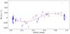 |
Fig. 1 Phase-folded RV data (blue) obtained with HIRES along with best-fit circular orbit model (solid red). One outlier is marked inred. |
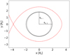 |
Fig. 2 Roche geometry of the planetary body (solid black) and Roche lobe (red dashed) of HAT-P-32 b. The dotted black line indicates a sphere with the perpendicular radius. The star is to the left. |
2.2 Roche geometry
The Roche potential depends on the positions and the mass ratio, q, of the bodies (e.g., Hilditch 2001)3. For HAT-P-32 b, we obtained a mass ratio of (4.81 ± 0.31) × 10−4 (Table 1), and the resulting geometry of the planetary Roche potential is shown in Fig. 2.
The planetary radius perpendicular to the star-planet axis is known from primary transit photometry and determines the equipotential surface defining the planetary surface. The planet is slightly elliptical with its radius along the symmetry line, Rp,∥, being about 8% larger than the perpendicular radius. The effective radius, Rp, eff, of a sphere with the same volume is 1.03 Rp,⊥. We use this value to derive the mean planet density of 0.135 ± 0.016 g cm−3 quoted in Table 1.
The height of the first Lagrange point above the surface is 1.140 ± 0.015 Rp,⊥. The secondLagrange point is slightly further up at 1.219 ± 0.016 Rp,⊥. In the perpendicular direction, the limit of the Roche lobe is closer to the planetary surface at a height of 0.435 ± 0.010 Rp,⊥ in the orbital plane. Consequently, the annulus of a Roche-lobe filling planetary atmosphere would cover
 (1)
(1)
of the stellar disk during lower conjunction. The effective radius of the Roche lobe is 1.526 ± 0.034 Rp,⊥ (Eggleton 1983), so that the planetary Roche lobe filling factor (by volume) becomes 30%.
3 CARMENES observations and data reduction
We obtained two transit time series of HAT-P-32 b on the nights of 1 September and 9 December 2018, in the following referred to as night 1 and night 2, with the CARMENES spectrograph. The CARMENES instrument is installed at the 3.5 m telescope of the Calar Alto Observatory in Spain and features a visual (VIS) and a near-infrared (NIR) arm, covering the 560–960 nm and 960–1710 nm range with a spectral resolution of 94 600 and 80 400, respectively (Quirrenbach et al. 2018). In accordance with its prime purpose as a planet finder, both arms are highly stabilized. CARMENES is fed with two fibers, of which the first was pointed at the target, HAT-P-32, and the second at the sky during our observations.
On nights 1 and 2, 23 and 26 usable science spectra were obtained, respectively, with an exposure time of about 900 s. On night 2, two observations had to be aborted after 640 s and 220 s because of technical difficulties. These are not considered in our analysis. In Tables A.1 and A.2, we list a log number (LN), the central time of exposure, the corresponding temporal offset from the center of the optical transit, the exposure time, and the overlap fraction of the planetary with the stellar disk averaged over the exposure for all spectra analyzed here.
3.1 Data reduction
The CARMENES data were reduced with the caracal pipeline (CARMENES Reduction And CALibration, Zechmeister et al. 2014; Caballero et al. 2016). In Fig. 3, we show the time evolution of the S/N in the spectral orders covering the Hα line in the VIS arm and the He I λ10833 triplet lines in the NIR arm as computed by caracal. While the S/N remained rather stable during night 1, it shows a decrease during night 2, which is particularly pronounced in the NIR data.
The stellar M1.5V-type companion, HAT-P-32 B, is located at a distance of 2.9″ from HAT-P-32 A. Although the CARMENES fibers provide a 1.5″ diameter acceptance angle (Quirrenbach et al. 2018), which separates the sources, some contamination from overlap of the seeing disks may be expected.On the basis of the results by Zhao et al. (2014), we estimate that the maximum possible flux contribution of HAT-P-32 B in the Hα and He I λ10833 spectral regions, obtained by assuming perfect overlap of the seeing disks, is 0.4% and 2.5% given (continuum) contrasts of about 6 mag and 4 mag. We expect the true contamination to be considerably smaller due to the angular separation of the targets. In early-type M dwarfs, the stellar He I λ10833 lines tend to be in absorption and rather stable (Fuhrmeister et al. 2019, 2020). In the hypothetical case of strong line contamination, for instance,owing to flaring, we expect of course no relation to the actual planetary transit timing. We, therefore, conclude that HAT-P-32 B is of little concern to our spectral analysis.
The regions around the Hα line and He I λ10833 triplet lines are affected by telluric water absorption lines. The He Iλ10833 infrared triplet region is additionally affected by OH emission lines. We corrected the water absorption lines in the optical and infrared using the molecfit package (Smette et al. 2015; Kausch et al. 2015). To remove the OH emission lines, we subtracted a semi-empirical synthetic model of the sky emission spectrum from the science spectra. This model was calibrated using a sample of 1836 observations of sky emission obtained by CARMENES. A detailed account of our telluric correction is given in Appendix B.
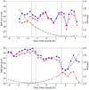 |
Fig. 3 Signal-to-noise ratio per pixel in order 93 of the VIS arm (blue circles) and order 56 of the NIR arm (red triangles) along with airmass (black, crosses) as a function of time for night 1 (top) and night 2 (bottom). Dashed, vertical lines indicate first and fourth contact and dotted, vertical lines the second and third contact. |
3.2 Radial velocity of HAT-P-32
To determine RV shift of the HAT-P-32 system, we fitted the spectral range from 8480 to 8700 Å, which contains thestrong lines of the Ca II IRT, using a PHOENIX model spectrum calculated for an effective temperature of 6200 K, surface gravity log(g) of 4.5, and solar metallicity from the grid presented by Husser et al. (2013). Prior to the fit, the template was broadened to account for stellar rotation (Table 1) and instrumental resolution. We then fitted all individual spectra, varying the stellar RV and the parameters of a second degree polynomial representing the continuum in the fit.
With this procedure, we determined an RV shift with respect to the PHOENIX model spectrum for all observed spectra. Fitting a circular model for the planetary orbital motion with fixed semi-amplitude (K⋆, Table 1) and free RV offset to these values, we found a mean value of  km s−1 for the RV shiftof the spectrum of HAT-P-32 with respect to the PHOENIX model spectrum at orbital phase zero. In this step, we neglected the contribution of the Rossiter-McLaughlin effect, which is small in amplitude in HAT-P-32 (≈100 m s−1, Albrecht et al. 2012). The quoted uncertainty is statistical. The value may be compared to the measurement of − 23.21 ± 0.26 km s−1 obtained with the Digital Speedometer (e.g., Latham 1996) and reported by Hartman et al. (2011), pointing to a true uncertainty including systematics on the order of 1 km s−1.
To cross-check our result, we fitted the 8130 to 8175 Å range in the VIS channel and the 11 040 to 11 075 Å range in the NIR channel with a synthetic, telluric water absorption model. For both channels and nights, we obtained offsets < 75 m s−1 with no considerable shifts within or between the nights. We conclude that the absolute wavelength calibration of the instrument is accurate to at least 75 m s−1 during our observations. The accuracy is probably better (Lafarga et al. 2020), but this value is sufficient for our analysis.
4 Stellar activity and planetary irradiation
Stellar activity plays an important role in exoplanetary research. In the planetary atmosphere, activity-induced irradiation acts as a driving force for the physics and chemistry. In planetary transmission spectroscopy, the role of activity phenomena is mostly one of a nuisance, in particular, because short-term variations in activity sensitive lines can mask or even mimic a planetary signal.
4.1 X-ray observations and planetary irradiation
We observed HAT-P-32 with XMM-Newton on 30 August 2019 through the DDT proposal ID 85338 (P.I.J. Sanz-Forcada) for an overall exposure time of 20.1 ks. The XMM-Newton satellite is equipped with three X-ray telescopes (Jansen et al. 2001) with three CCD cameras at their focal planes, provided by the European Photon Imaging Camera (EPIC) consortium. The assembly consists of two metal oxide semi-conductor (MOS) CCD arrays and one array of so-called pn-CCDs (Strüder et al. 2001; Turner et al. 2001), whose fields of view largely overlap, so that they are usually operated simultaneously.
During our observation, the EPIC pn and MOS X-ray detectors were partly affected by high background, which was removed prior to the spectral analysis. The EPIC cameras do not provide sufficient spatial resolution to separate the stellar A and B components, but the optical monitor (OM) on board XMM-Newton indicates that uv emission in the UVW2 filter (λc = 2120 Å) comes from the F-type main component, with no emission detected from the M dwarf companion. EPIC light curves indicate the presence of flares (Sanz-Forcada et al., in prep.), which most likely come from the primary star in the system.
We performed a simultaneous spectral fit to the three EPIC spectra, with a S∕N = 11.3. A single coronal plasma model component with a temperature, log(T (K)), of 6.61 ± 0.08 and an emission measure, log (EM (cm−3)), of 51.90 ± 0.10 and its metal abundances fixed to the slightly subsolar photospheric value of [Fe/H] = −0.04 suffices to fit the spectra. The X-ray luminosity of the system is LX = 2.3 × 1029 erg s−1 in the 5–100 Å range. Assuming that most X-ray flux originates from the primary, this translates into log LX∕Lbol = −4.5, which is a relatively high value, especially for an F star (e.g., Pizzolato et al. 2003). The X-ray light curve shows a moderate level of short-term variability most likely attributable to X-ray flaring on the main component; a detailed analysis will be published elsewhere (Sanz-Forcada et al. in prep.).
We extended the coronal model toward cooler temperatures following Sanz-Forcada et al. (2011). This model was then used to predict the spectral energy distribution at wavelengths up to 1600 Å. The model flux in the XUV spectral ranges relative to the He and H ionization edges are  erg s−1 (100–504 Å) and
  erg s−1 (100–920 Å). From our modeling, we obtain a total XUV (< 912 Å) flux of ≈ 4.2 × 10⁵ erg cm−2 s−1 at the planetary orbit. To further extend the model and calculate the NUV irradiation level, we employ a photospheric model (Castelli & Kurucz 2003). We here define the NUV as the 912–3646 Å range, bracketed by the onset of Balmer continuum absorption at its red boundary. For the NUV irradiation at the planetary orbital distance, we obtain ≈ 6 × 10⁷ erg cm−2 s−1.
The XUV emission of HAT-P-32 is about 100 times solar and results in an extremely high-energy irradiation environmentfor the planet, which is expected to produce substantial atmospheric mass loss from HAT-P-32 b. In this particular case, the loss rate is increased by mass flow through the Roche lobe (Erkaev et al. 2007). Under an energy-limited escape model (Sanz-Forcada et al. 2011, and references therein), we estimate a mass-loss rate of 1014 g s−1. The statistical uncertainty of this value is driven by the irradiating flux and amounts to about a factor of two, which does not account for variability in the XUV flux. Adopting an evaporation efficiency of 0.1 for a gravitational surface potential of log (Φ(erg g−1)) = 12.8 from Salz et al. (2016b) reduces the mass-loss rate to 1013 g s−1, which remains an extremely high value.
4.2 Variability analysis of the Ca II IRT triplet lines
Both the He Iλ10833 triplet lines and the Hα line are sensitive to activity-related changes in the chromosphere (e.g., Fuhrmeister et al. 2018, 2019). Likewise, the Ca II IRT lines are well-known tracers of chromospheric activity (e.g., Martin et al. 2017). While planetary atmospheric absorption has been observed in these lines also (Yan et al. 2019), this has only been in planets with considerably higher surface temperatures so far.
In Fig. 4, we show the light curve obtained for the three components of the Ca II IRT triplet as well as a mean Ca II IRT light curve. To obtain these light curves, we normalized the spectra in the region of the lines and summed the normalized flux in bands with half-widths of 0.2 Å centered on the nominal positions of the Ca II IRT lines.
No flaring activity, which would be characterized by a fast rise phase and longer decay phase in the Ca II lines (e.g., Klocová et al. 2017), can be distinguished in these light curves. Also no signal associated with the transit itself is observed. The Ca II IRT lines are consistent with a constant level of activity during night 1. On night 2, some systematic evolution may be present in the Ca II IRT lines, indicating a slightly elevated activity level during the transit compared to before and after the transit. However, the amplitude of variability remains within the limits of the scatter observed on night 1. We conclude that stellar activity, as far as it manifests itself in the Ca II IRT lines, is not a strong interference in our data sets.
5 Hα and He I λ10833 transmission spectroscopy
To study the planetary transmission spectrum, we started with the spectra corrected for telluric line contamination and shifted them according the barycentric motion of the Earth. We then normalized the spectral ranges covering the He I λ10833 and Hα lines using a linear fit to the surrounding continuum. The spectra thus obtained are referred to as fn,i (λ), where n ={1, 2} specifies the night and i denotes the LN. In Fig. 5, we show a heat map4 of the spectral time series around the He Iλ10833 line on night 1. Already in this map, an absorption signal aligned with the planetary track both in RV and transit timing can be discerned.
 |
Fig. 4 Normalized Ca II IRT light curves of individual triplet components (blue dashed, red dash-dotted, and green dotted in order of ascending wavelength) along with the mean light curve (black solid). First to fourth contact times are indicated, and the neutral line is at one. |
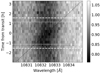 |
Fig. 5 Heat map showing the time series of normalized spectra around the He I λ10833 triplet lines on night 1. Optical transit contacts (horizontal dashed and dotted lines) and the planetary RV track (black dashed) are indicated. |
5.1 Reference, transmission, and residual spectra
To work out the signature of the planetary atmosphere more clearly, we constructed reference spectra by averaging a number of suitable out-of-transit spectra. In particular, we chose subsets of our spectra 2.2 h or more before and after the center of the optical transit for each night. If  denotes a suitable subset of LNs to be considered for night n and spectralline L, which either refers to Hα or He I λ10833 here, we construct a reference spectrum, R, by averaging
 (2)
(2)
where  is the number of spectra in the set. As the stellar rotational line width is much larger than the effect caused by the stellar reflex motion, we neglect the effect here.
After careful examination of the spectral time series on nights 1 and 2, we constructed reference spectra for the Hα and He I λ10833 line regions for both nights, using the ranges of spectra listed in Table 2 (see Appendix C for details). In all but one case, we opted for a combination of pre- and post-transit spectra. Only for the He I λ10833 line region on night 2, we prefer to use only pre-transit spectra to avoid residual effects due to strong contamination by OH emission lines, which is otherwise well accounted for (Appendix B). Using the reference spectra, individual empirical transmission spectra, tn,i, are obtained according to
 (3)
(3)
where λL indicates a suitable wavelength range around the spectral line indicated by L. Finally, we call rn,i = tn,i − 1 a residual spectrum. All of fn,i, rn,i, and tn,i refer to the barycentric frame. The systemic velocity of the HAT-P-32 system is not accounted for.
A signal originating in the planetary atmosphere is shifted in RV by the orbital motion of the solid planetary body, potential velocity fields within the planetary atmosphere, and the velocity of the system’s barycenter, which we assume to be constant (Sect. 3.2); the effect of the secular acceleration of the HAT-P-32 system is around − 10 m s−1 between the two nights (see Sect. 2.1), which we consider negligible. To study the behavior of the signals in the co-moving planetary frame (i.e., the planetary rest frame moving along with the planetary system), we obtained shifted residual spectra,  , by applying a Doppler shift offsetting the planetary orbital motion (see, e.g., Wyttenbach et al. 2015). The applied RV shift corresponds to that during the middle of the respective observation; the treatment of finite integration times is discussed in Sect. 6.2.
Log numbers of spectra used to construct reference spectra.
5.2 Residual maps
In Figs. 6 and 7, we show the time evolution of the residual spectra, rn,i, for the Hα and He I λ10833 lines on nights 1 and 2 in the form of heat maps along with a map combining the data of the two nights. In the He I λ10833 residual map for night 2, we masked the post-transit residuals associated with the strong Q1 OH emission line doublet (see Table B.1).
The He Iλ10833 maps show a pronounced absorption signal, which is associated with the optical transit in terms of timing and moves along with the planetary RV track. A signal with similar properties but less pronounced is also seen in the Hα maps. The properties of the absorption signals, therefore, point to an origin in the planetary atmosphere.
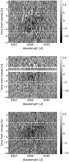 |
Fig. 6 Heat maps of the Hα line region for night 1 (top), night 2 (middle), and a combination of both (bottom). The color bar encodes the amplitude of the residuals in percent. |
5.3 Time-resolved transmission spectra
To study the temporal evolution of the transmission spectrum, we defined six time intervals, which we call pre-transit, ingress, start, center, end, and egress and identify the spectra of nights 1 and 2 belonging to the individual sections. In Fig. 8, we show the temporal coverage resulting from our attribution scheme; a detailed account for the individual spectra is given in Tables A.1 and A.2. Our temporal sampling of about 15 min and cadence shifts due to technical problems limit the accuracy with which individual sections can be separated and aligned on nights 1 and 2.
We obtained transmission spectra by coadding the shifted residual spectra,  , pertaining to the sections under consideration (see, e.g., Wyttenbach et al. 2015). Our transmission spectra were corrected for planetary orbital motion, but not for the systemic RV shift of the whole HAT-P-32 system. The resulting time-resolved transmission spectra are shown in Figs. 9 and 10 for the Hα and He I λ10833 lines. For each line and section, we show the transmission spectrum obtained on night 1 and night 2 as well as an averagedspectrum. In Fig. 11, we juxtapose the averaged transmission spectra for the Hα and He I λ10833 line regions. The shown transmission spectra were smoothed by a running mean with a window width of 0.165 Å for the Hα and 0.2 Å for the He I λ10833 lines.
Both the He Iλ10833 and Hα line transmission spectra show pronounced absorption signals primarily during the start, center, and end phases. The signals are broad with respectto the instrumental resolution and approximately in the planetary rest frame. The central dip of the He I λ10833 transmission spectrum reaches a depth of around 6% during the start and center phase. During the end phase, which is nearly symmetric to the start phase in terms of the geometry of the star-planet system, the central He I λ10833 transmission dip is weaker, reaching a depth of about 4%. For Hα the maximum depth of around 5% is also observed during the center phase. In Table 3, we give the EWs of the night-averaged transmission signals in the − 100 km s−1 to + 100 km s−1 range along with an estimate of the uncertainty obtained from repeated reshuffling of the transmission spectra.
According to the Roche geometry (Sect. 2.2), a Roche-lobe filling atmosphere covers about 2.4% of the stellar disk, which is less than the depth of absorption observed either in Hα or the He I λ10833 lines. It thus follows that Roche-lobe overflow must play a role in the HAT-P-32 system.
The time series of transmission spectra shows a complex pattern of variability, which may be associated with the three-dimensional overflow geometry. Notably, the He I λ10833 transmission spectrum displays pronounced absorption, redshifted by about 25 km s−1 with respect to the planetary body, before the optical transit commences. In this pre-transit phase, no absorption at the nominal wavelength of rest of the He I λ10833 lines is detectable. A similar He I λ10833 absorption component is present during the ingress phase, yet, slightly shifted toward the line center. Another absorption component redshifted by about 70 km s−1 can be discerned during ingress, which is consistently observed in both nights. During the ingress phase, the He I λ10833 absorption component extends to redshifts of about 100 km s−1. This component appears to persist into the start phase, where it is discernible at a weaker level. The He I λ10833 egress absorption is weaker than its ingress counterpart. Particularly during the end phase, a blueshifted absorption component is visible, which appears in both lines, but is narrower in the case of the Hα line (Figs. 9 and 11). However, absorption is weak (He I λ10833) or absent (Hα) during the egress phase and no post-transit absorption is detectable.
Overall, the transmission in the Hα line is comparable to or weaker than that in the He I λ10833 lines. The behavior of the red flank of the Hα line transmission spectrum is similar to that of He Iλ10833 during the ingress and start phases. The Hα line transmission spectrum during the pre-transit phase, however, shows a weaker absorption component, if any (cf., Sect. 5.5).
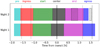 |
Fig. 8 From left to right, the pre, ingress, start, center, end, and egress sections, as indicated by the colored areas. Hatched sections on night 2 refer to technical dropouts. Dashed and dotted lines show the four contact times. |
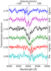 |
Fig. 9 Hα transmission spectra for ingress, start, center, end, and egress phase from bottom to top (consecutively offset by 0.05; comoving planetary frame). Dashed lines show night 1 results, dotted lines night 2 results, and solid lines the average of these two. |
Equivalent widths of transmission signals in −100 km s−1 to + 100 km s−1 range as a function of transit phase.
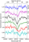 |
Fig. 10 Transmission spectra in the He Iλ10833 line region for ingress, start, center, end, and egress phase from bottom to top (consecutively offset by 0.05; comoving planetary frame). Dashed lines show night 1 results, dotted lines night 2 results, and solid lines the average of these two. |
5.4 Center-to-limb variation
During the transit, the opaque planetary disk consecutively covers different sections of the stellar photosphere, seen at changing viewing angles and rotational shifts, which produces a signal in the transmission spectrum (e.g., Czesla et al. 2015; Yan et al. 2015). Following Salz et al. (2018), we refer to this signal as a pseudo-signal. It can have far-reaching ramifications for the interpretation of the transmission spectrum as has been shown, for example, by Salz et al. (2018) and Casasayas-Barris et al. (2020).
To determine the strength of the pseudo-signal expected to be caused by the center-to-limb variation (CLV) in HAT-P-32, we simulated the transmission spectrum of the opaque planetary disk using the methodology presented by Czesla et al. (2015). The simulations are based on a discretized stellar surface and synthetic specific intensities derived using Kurucz stellar model atmospheres (Castelli & Kurucz 2003) and the spectrum program by R.O. Gray (Gray & Corbally 1994). Based on these inputs, a spectrum is then synthesized for every phase of the transit. In Fig. 12, we show the resulting synthetic transmission spectra produced by the transit of the opaque planetary disk during the sections indicated in Fig. 8.
As is shown in Fig. 12, the effect of the CLV is mostly one of pseudo-emission, which is strongest during the center phase of the transit but also then remains ≤ 0.7%, with a baseline of about 0.2% belonging to a broad component, attributable to the broad Hα line. During the transit, the most distinct predicted signal evolves mostly within the − 50 km s−1 to 50 km s−1 range in the stellar rest frame. Analogous predictions for the He I λ10833 are naturally limited by the fact that the He Iλ10833 is not included in photospheric synthetic models and has basically unknown limb-angle dependence. However, as the stellar He I λ10833 line is considerably weaker than the Hα line in HAT-P-32, we expect also a weaker effect. Compared to the observed Hα and He I λ10833 transmission signals, the CLV-induced pseudo-signals are a secondary effect in HAT-P-32 b and do not significantly affect the interpretation of the observed signals.
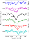 |
Fig. 11 Superimposed transmission spectra in He Iλ10833 (solid) and Hα (dashed) for ingress, start, center, end, and egress phase from bottom to top (consecutively offset by 0.06). |
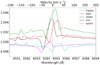 |
Fig. 12 Synthetic (pseudo-)transmission signals caused by the CLV during individual temporal sections of the transit. |
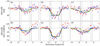 |
Fig. 13 Transmission light curves for Hα (top row, panels a–c) and He Iλ10833 (bottom row, panels d–f) for velocity bands (−50, −15) km s−1, (−15, +15) km s−1, and (+ 15, +50) km s−1 from left to right. Blue diamonds indicate night 1 and red circles indicate night 2. The solid yellow lines represent best-fit light curves from the circumplanetary annulus model, dash-dotted black lines are model light curves pertaining to the super-rotating wind model, and the green solid lines are those for the combined circumplanetary and up-orbit stream model. |
5.5 Transmission light curves
To investigate the time evolution of the transmission signal from a different perspective, we constructed transmission light curves by integrating the residual spectra in the co-moving planetary frame
 (4)
(4)
We here chose three wavelength ranges, representing the blue flank, the core, and the red flank of the transmission spectra shown in Figs. 9 and 10. The adopted ranges correspond to Doppler shifts between − 50 and − 15 km s−1, − 15 and + 15 km s−1, and +15 and + 50 km s−1 with respect to the nominal wavelengths of the Hα and He I λ10833 lines, and the resulting light curves are shown in Fig. 13.
The light curve of the He Iλ10833 core (panel e; dashed lines) shows a pronounced depression during the optical transit with an EW reaching about 60 mÅ. The Hα line core shows a comparable behavior with a signal of about 25 mÅ; as the same velocity band is about 65% broader around He Iλ10833 than Hα in wavelength units, the difference in signal depth is smaller. The He Iλ10833 core light curve on night 2 does not return to the pre-transit level after the optical transit. This behavior is even more pronounced in the blue-flank He I λ10833 light curve (panel d), but it does not occur on night 1. We therefore attribute this to residual effects caused by the telluric OH emission line doublet, which becomes considerably stronger on night 2 after the optical fourth contact (see Fig. B.5). Of course, this effect has also to be present in the transmission spectra shown in Fig. 10, and, indeed, the red flank of the night 2 transmission spectrum shows higher levels than those on night 1. Compared to the overall strength of the transmission signal, the difference remains modest, however.
The red-flank He Iλ10833 light curve (panel f) shows a prominent early ingress, starting about one hour before the first optical contact. The early ingress is seen in the data of both nights, although the night 1 light curve barely captures the start of the depression, it is well sampled by the longer pre-transit coverage offered by the night 2 light curve. The red-flank Hα and He I λ10833 light curves are consistent with an early egress, starting before the third optical contact. The night 2 He I λ10833 light curve shows a stronger effect here, even turning into apparent residual emission, which may again be caused by the strong OH contamination. Yet, both light curves return to the pre-early-ingress level after the transit. Inspecting the red-flank Hα light curve, a similar pattern can be discerned. These light curves display the early egress rather well, which commences close to the center of the optical transit. An early ingress may be discernible as well, although the light curves of both nights show an upward excursion shortly before the first optical contact, making the situation less clear in this case.
6 Phenomenological transmission spectrum modeling
In both observing nights, we detect strong, consistent absorption signals in both the Hα and the He I λ10833 triplet lines in HAT-P-32 b. The lines show substructure and distinct temporal variation, which we attribute to the distribution of absorbing material in the system.
In the corotating star-planet frame, mass is subject to gravitational and centrifugal forces that can be combined into the scalar Roche potential, and any moving material is also subject to the Coriolis force. As shown, for instance, by Bisikalo et al. (2013) and Carroll-Nellenback et al. (2017), the combined effect of these forces can deflect a hydrodynamic planetary wind into a two-stream geometry. According to Carroll-Nellenback et al. (2017), an up-orbit stream, launched mainly from the planetary dayside, precedes the planet and is directed toward the interior of the planetary system, where it can lead to the formation of a circumstellar disk by stream-stream interaction or may eventually be accreted onto the star (Lai et al. 2010). A down-orbit stream, launched mainly from the planetary nightside, trails the planet, resembling a cometary tail. Such a two-stream geometry has, indeed, been inferred from optical photometric observations in K2-22 b, where, however, the material is in a different physical regime (Sanchis-Ojeda et al. 2015). Further agents such as stellar wind interaction, radiation pressure, and magnetic fields can significantly modify the geometry (e.g., Ehrenreich et al. 2015; McCann et al. 2019; Daley-Yates & Stevens 2019).
Mostly focusing on the HD 209458 system, Carroll-Nellenback et al. (2017) also show simulations as a function of the planetary radius expressed in terms of the sonic radius, rs, of the Parker wind,  , and the ratio, τ, of Parker time and orbital time
  , where vS is the speed of sound and Ω is
  . Adopting 10 km s−1 for vs (Sect. 7.2), we estimate (Ξp, τ) ≈ (0.3, 1.5) for HAT-P-32 b, which indeed leads to the formation of up- and down-orbit streams in their model. The geometry described by Carroll-Nellenback et al. (2017) shows some of the same features as the geometry described by Lai et al. (2010) and Li et al. (2010), who adapted the theory of Roche lobe overflow in semidetached binary stars (Lubow & Shu 1975) to describe a stream launched through the first Lagrangian point.
Apart from the structure of the outermost atmosphere, other components of the planetary atmosphere that may contribute to the observable transmission signal include super-rotating winds, which may cause Doppler-broadened, shifted, or even split transmission signals. A super-rotating atmosphere exhibiting such properties has, for example, been reported for HD 189733 b (e.g., Knutson et al. 2007; Louden & Wheatley 2015; Salz et al. 2018).
In the following, we model the observed transmission spectra using two alternative assumptions on the geometry of the absorbing material, inspired both by the morphology of the signals and the models cited above. First, we assume that only a circumplanetary atmosphere with potential (super-)rotation is responsible for the observed signals. Second, we assume that an up-orbit stream is also present as described by Lai et al. (2010) and Carroll-Nellenback et al. (2017). Dedicated one-dimensional hydrodynamic modeling of the atmosphere of HAT-P-32 b is presented in Sect. 7.
6.1 Calculation of synthetic transmission spectra
We calculated synthetic transmission spectra with an approach similar to that used by Salz et al. (2018). The absorption cross section per atom, σ(λ), was modeled using Gaussian profiles, G, parameterized by the rest wavelength, λ0, a velocity shift, vs, the oscillator strength, f, and the velocity dispersion, vd. The oscillator strength and rest wavelength were adopted from Drake (2006) and the National Institute of Standards and Technology (NIST, see Table 4). For the He I λ10833 lines, we used a superposition of three components for the cross section so that
 (5)
(5)
If (non-overlapping) fractions, fj, of the stellar disk (measured in units of the disk area) are covered by absorbers with local column densities nj producing optical depths nj σj(λ), the empirical transmissionspectrum, T, is approximated by
 (6)
(6)
where Rinst * represents convolution with the instrumental profile, which we assume to be Gaussian. In this approach, the stellar disk is treated as a homogeneous source of light, neglecting CLV and other sources of inhomogeneity (Czesla et al. 2015; Yan et al. 2015).
It is computationally convenient to apply the instrumental broadening directly to the optical depth profile
 (7)
(7)
The first two orders in the Taylor expansion of the resulting expression are identical to that of the original one (Appendix G). The approximation is, thus, accurate in the optically thin limit. In our phenomenological modeling, optical depths on the order of one have to be dealt with and the instrumental resolution is high compared to the line width. Therefore, higher-order corrections terms remain small and can be neglected.
The observationally obtained transmission spectra corresponding to the six orbital phase ranges defined in Sect. 5.3 all rely on the combination of two or more individual in-transit spectra, which correspond to different orbit configurations. To obtain synthetic transmission spectra, we first obtain model spectra appropriate for the mid-exposure time for all individual observations during nights 1 and 2. Subsequently, we average the synthetic spectra using the same scheme as that for the observations.
Line parameters adopted in the modeling.
6.2 Treatment of phase smearing
The problem of phase smearing is caused by the long exposure times (e.g., Ridden-Harper et al. 2016). A single exposure of 900 s comprises about 0.5% of the orbit of HAT-P-32 b or 8% of the optical transit duration. At mid-transit time, this means that the RV of HAT-P-32 b changes by 5.3 km s−1 during any single exposure due to the planetary orbital motion. Even assuming that the profile of the transmission spectrum remains constant during the exposure, which is not necessarily the case (Deming & Sheppard 2017), this effect distorts the observed line profile in the transmission spectrum compared to the instantaneous profile.
The effect of phase smearing can be taken into account in the modeling by applying a convolution with a box-shaped broadening kernel (Cauley et al. 2021; Wyttenbach et al. 2020). Here we used an effective value for the instrumental resolution, determined by evaluating the effect of the box-shaped convolution on the instrumental broadening function. An appropriate value can be derived by demanding that the variance of the profile resulting from time integration is reproduced. The result remains an approximation in the sense that we reproduce the variance but not necessarily the profile; an in-depth discussion of the role of instrumental resolution in transmission spectroscopy can be found in Pino et al. (2018). In the case of HAT-P-32 b, effective values of 63 000 and 58 000 for the instrumental resolution fulfill this condition for the VIS and NIR channels of CARMENES (see Appendix D).
6.3 Circumplanetary atmosphere and super-rotation
First, we approximated the planetary atmosphere by a face-on annulus, which surrounds the opaque disk of the planet, reaching from the planetary surface at Rp,⊥ to an outer radius Ra,out. We assumed constant surface column densities, Na, of absorbers in the Hα and He I λ10833 lines. As shown in Sect. 7, the true atmospheres show a distribution of column densities. Therefore, the value derived here should be understood as an effective number, representing the value reproducing the line profile best. The material in the atmospheric annulus is dragged along with the planetary frame. In a first step, we allowed for broadening with velocity vt,a, which captures all broadening mechanisms and, in a second step, we considered (super-)rotation of the planetary atmosphere with equatorial wind velocity vw and the planetary equator lying in the orbital plane. To get an idea of the amount of absorbing material and the broadening of the lines, we here assumed an atmosphere with a fixed maximum stellar disk coverage fraction of 10%, corresponding to an outer radius of 2.3 Rp,⊥. As long as no strong saturation effects or timing effects due to the extent of the atmosphere occur, the values of the atmospheric fill factor and surface column density remain largely degenerate. Treating the surface column density and the turbulent velocity as free parameters, we carried out a fit by minimizing χ2 using the transmission spectra for each of the phases simultaneously. The fit results for the individual sections of the transit, as well as a comparison by means of the Bayesian information criterion (BIC) are given in Tables F.1 and F.2. The best-fit spectral models are shown in Fig. 15 and the corresponding transmission light curves are indicated in Fig. 13.
Allowing also the planetary equatorial wind velocity, vw, to vary, yields an overall better fit, which is mainly driven by the ingress phase (Table F.1). This may be expected, because this phase is where the asymmetry in the atmospheric motion is most pronounced. The weak signal in the egress phase does not yield a strong lever to distinguish the models. The best-fit wind velocity is around 23 km s−1 for the Hα and He I λ10833 lines independently, and the turbulent velocity is diminished because some of the broadening is absorbed by the atmospheric wind motion (Table 5).
Clearly, this model reproduces the main depression in the transmission spectrum in both lines, but it can neither explain the difference between the observed central depression during the start and end phases, as the star–planet geometry is symmetric, nor does it provide an explanation for the pre-transit absorption signal or theline wings. This is also reflected by the associated transmission light curves in Fig. 13, which are reasonable for the line center, but significantly off for the line wings (see panels c and f in particular). Taking the coverage fraction of the atmosphere into account, we converted the column densities from Table 5 into a total number of (4 ± 0.3) × 1033 Hα absorbers and (4.7 ± 0.4) × 1033 He I λ10833 absorbers, which corresponds to (6.8 ± 0.6) × 109 g and (3.2 ± 0.3) × 1010 g, respectively.
 |
Fig. 14 Sketch of the HAT-P-32 system (approximate scales). The planetary body (black circle) moves along its orbit (solid line). The direction of orbital motion is indicated by an arrow head. The planetary body is surrounded by an atmosphere (gray shade). The model up-orbit stream (black rectangle) originates from the first Lagrange point. |
Best-fit parameters for annulus, super-rotating wind, and up-orbit stream models. Reduced χ2 values,  , are calculatedover the −100to+100 km s−1 range.
6.4 Circumplanetary atmosphere plus up-orbit stream
In a next step, we extended the circumplanetary (annulus) atmosphere model by a semi ad hoc version of the up-orbitstream model presented by Lai et al. (2010). The geometry is depicted in Fig. 14. From the first Lagrange point, the up-orbit stream is launched toward the interior of the planetary system. In the theory of Lubow & Shu (1975) adopted by Lai et al. (2010), the launching angle is about 30° with respect to the radius vector of the planetary body, but Coriolis forces tend to increase that angle. The final geometry depends on the physical stream conditions as well as the interaction with the environment.
As detailed physical stream modeling is beyond our scope, we assumed a fixed, intermediate value of 45° for the stream angle in our phenomenological modeling. For the stream, we assumed a quadratic cross section, constant along the stream, with an edge length equal to the diameter of the planet (2Rp,⊥). We fixed thetotal length, Ls, of the stream at 1.5 stellar radii in our modeling. While we did not treat the stream length as a free parameter, we note that it is constrained by the ingress timing. Conceivable physical factors limiting the stream length are the presence of a circumstellar disk formed by self-interaction of the stream or stellar wind interaction (e.g., Lai et al. 2010). The streaming velocity was assumed to increase linearly with the distance, l, from the L1 point along the stream, starting from a minimal velocity, vmin, of 5 km s−1 (set by the speed of sound, Lai et al. 2010) to a maximum velocity, vmax. If ṅk is the number of particles of type k streaming through any perpendicular cross section of the stream with area A per unit time, then continuity requires that
 (8)
(8)
where ρk(l) is the volume particle density. Here, we neglect that the number density of Hα and He I λ10833 absorbers may change due to (de-)excitation along the stream. Integration yields the total number of particles in the stream
 (9)
(9)
In our modeling, we only treated vmax and ns,k as free parameters. The best-fit parameters are given in Table 5, and the best-fit spectral models and associated transmission light curves are shown in Figs. 13 and 15.
The up-orbit stream model considerably improves the fit to the transmission spectra. In particular, the pre-transit depression can now be modeled and the red-wing line profile is better approximated compared to the circumplanetary atmosphere model alone. This is also clearly seen in the associated transmission light curves shown in Fig. 13. Formally, the improvement in  is highly significant with an F-test yielding p-values smaller than10−6. While the fit is significantly better, we caution that this does not prove the correctness of the model.
Compared to the previous model, both the best-fit values of the surface column densities and the turbulent velocities are decreased, because some absorption and broadening is now accounted for by the stream component. The maximum stream velocities of 90 km s−1 and 131 km s−1 for the Hα and He I λ10833 components are roughly compatible with the model prediction of less than half of the planetary orbital speed of about 90 km s−1 for HAT-P-32 b given by Lai et al. (2010). Based on our modeling, we obtain streaming rates of (6.6 ± 1.7) × 104 g s−1 and (6.3 ± 1.1) × 105 g s−1 of Hα and He I λ10833 absorbers.
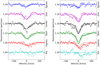 |
Fig. 15 Average transmission spectra along with best-fit models for annulus atmosphere (dashed), super-rotating wind (dotted), and up-orbit stream (solid) for the Hα line (left) and the He Iλ10833 lines (right). |
6.5 Limits of the model and further components
Although our phenomenological modeling accounts for the main characteristics of the observed transmissions spectra, not all aspects are captured. In the following, we outline those aspects along with some speculative explanations.
The depth of the central part of the He I λ10833 transmission spectrum decreases between the start and end phase of the transit (Fig. 10), which may be accounted for by an asymmetric model component such as the streaming funnel. In our implementation, however, the observed decrease in depth of the central He I λ10833 component is not reproduced. Nonetheless, effects caused by the changing line of sight through a potentially asymmetric and at least partially optically thick atmosphere as well as occultation of parts of the atmosphere by the opaque planetary disk provide a conceivable explanation for the observation. Also heterogeneities in an hypothetical circumstellar disk formed by self-interaction of the up-orbit stream and its impact on the disk may contribute to the observed transmission spectrum (Lai et al. 2010), including the changing depth of the central absorption over the transit.
Particularly during the end phase of the transit, a blueshifted absorption component at a velocity of around − 50 km s−1 appears to be present, which is not accounted for by our modeling. This signal may be attributable to the weaker, bluest component of the He I λ10833 triplet, the contribution of which becomes stronger through absorption by larger column densities (Salz et al. 2018). Conceivably, material might also streams across the second Lagrange point after which it is accelerated away from the star, potentially forming a comet-like tail (e.g., Carroll-Nellenback et al. 2017; Nortmann et al. 2018). A high-velocity He I population produced by charge exchange with the stellar wind is also conceivable; however, we would expect that to be observable during the entire transit, which does not seem to be the case.
In the central transit phase, the Hα transmission line shows a central absorption component, which is deeper than that of the model. During the subsequent end phase of the transit, the Hα line transmission spectrum shows a marked double-peak structure, which is not observed during the start phase of the transit (Fig. 9). Such a structure may possibly be caused by a circumplanetary disk, seen nearly edge-on. However, the planetary Roche lobe is almost filled by the planetary body already (Sect. 2.2), leaving limited space for a gravitationally bound disk, and the signature would somehow have to be suppressed in the remaining transit phases.
7 Hydrodynamic atmospheric modeling
We now turn to hydrodynamic modeling of the atmosphere of HAT-P-32 b to further explore the properties of the outflow. To that end, we applied the two separate methodologies of García Muñoz & Schneider (2019) for the Hα line and that of Lampón et al. (2020) to investigate the He Iλ10833 lines. A joint analysis of the lines and their temporal variability based on hydrodynamic modeling is deferred to future work. Throughout this section, we refer to the center-phase transmission spectrum for the comparison with the models.
7.1 Modeling of the Hα transmission signal
We used the model developed by García Muñoz & Schneider (2019) to predict the population of hydrogen atoms excited into the H(2) state that causes the Hα absorption in the upper atmosphere of HAT-P-32 b. The model builds upon past approaches to hydrodynamic escape (García Muñoz 2007) by incorporating a non-local thermodynamic equilibrium (NLTE) treatment of the hydrogen atom, together with the description of the direct (stellar) and diffuse radiation components within the gas. The simultaneous solution to the continuity, momentum, and energy conservation equations allows us to trace the transition from a hydrostatic gas at the ~1 μbar pressure level to a rapidly escaping and much hotter gas at pressures of 0.02–0.03 μbars, where the Hα lines originate. The model is one-dimensional and takes the radial distance to the planet center as the only spatial variable in the equations. It takes as input the stellar spectrum described in Sect. 4.1. Particularly important are the energy fluxes incident upon the planet in the XUV (< 912 Å) and the NUV (912–3646 Å).
We set the base of the upper atmosphere in our models at the pressure level of 1 μbar. It is not straightforward to translate this into a radius Rp,1μbar because the transition from the ~mbar pressure level probed at optical and NIR wavelengths to the μbar level depends on the temperature and the dissociation/ionization state of the intervening gas, which is not well constrained. We estimated that Rp,1μbar/Rp = 1.1 and used this choice for our hydrodynamic calculations. We confirmed that the solution is not strongly sensitive to the specific choice. Our current version of the NLTE-hydrodynamic model includes atomic hydrogen (with excitation states up to the principal quantum number n = 5), protons and electrons but not molecular hydrogen, helium or other heavier atoms. Although the main features of the flow are dictated by the dominating hydrogen gas, as shown by García Muñoz (2007), the omission of helium prevents for the time being the direct comparison with the He I λ10833 line measurements.
Figure 16 (top panel) shows that temperatures of up to 18 000 K and supersonic velocities as high as 25 km s−1 are reached in the vicinity of the planet. From these simulations, we estimate that the planet is losing mass at a rate πρur2 = 1.4 × 10¹³ g s−1, where ρ is the density, u the velocity, and r the respective radius. Correspondingly, the middle and bottom panels show that most of the H(2) state is formed within a relatively narrow layer at ~1.8 planetary radii. In this region, the gas transitions rapidly from mostly neutral to mostly ionized, a fact that tends to maximize the excitation of H(2) from collisions of H(1) and electrons. This layer has an optical thickness at the line core well in excess of one and causes the high-altitude layer of Hα detected around the planet. Although the altitude and strength of this layer can be sensitive to a number of factors that will be explored in future work, it is apparent that both observations and model predictions are consistent (Fig. 17).
7.2 Modeling of the He Iλ10833 transmission signal
To analyze the He Iλ10833 absorption signal we used the model described by Lampón et al. (2020). The model has two major components, first, the solution of the hydrodynamical equations and, second, the computation of the NLTE population of the He (23S) excited state responsible for the planetary atmospheric absorption.
The hydrodynamical model is a variation of the isothermal spherically symmetric Parker wind approach (Parker 1958), with the main difference being that not the temperature but the speed of sound, vs, is assumed to be constant. This is given by
 (10)
(10)
where k is the Boltzmann constant, r is altitude, T(r) is temperature, and μ(r) denotes the mean molecular weight of the thermosphere. By construction, the thermosphere shows an altitude-independent T(r)∕μ(r) ratio. The value of the speed of sound is given by  , where
  is the averaged mean molecular weight, calculated in the model, and T0 is a free model parameter that is similar to the maximum of the thermospheric temperature profile calculated by comprehensive hydrodynamic models that solve the energy balance equation (e.g., Salz et al. 2016a; García Muñoz & Schneider 2019). A novelty of this hydrodynamical model is the way in which the averaged mean molecular weight is computed (see Eq. (A.3) in Lampón et al. 2020), which makes the convergence of the solution fast. In addition to the temperature T0, the model includes two other free parameters, the hydrogen-to-helium number ratio, and the atmospheric mass-loss rate, Ṁ, which here refers to the substellar value scaled by planetary surface area.
Along with the density and RV profile, the model yields the distribution of the species H, H+, He (11S) He+, and He (23S) by solving the hydrodynamical equations and their respective continuity equations. The production and loss terms of those species are detailed in Table 2 of Lampón et al. (2020). The computation of those quantities requires as input the stellar flux received at the top of the planetary atmosphere (see Sect. 4.1).
Based on the He (23S) radial distribution, the model computes the He (23S) absorption by using a radiative transfer code for the primary transit geometry (see Sect. 3.3 in Lampón et al. 2020). The absorption coefficients and wavelengths for the three metastable helium lines were taken from the NIST Atomic Spectra Database5 (see Table 4). The lines are assumed to have Gaussian Doppler line shapes with two broadening contributions, viz., thermal broadening and a second optional component, produced by turbulence with a velocity scale given by the speed of sound  , where m is the mass of a He atom. In addition to microscopic broadening, the model also accounts for the broadening of the lines caused by the bulk wind motion of the material in the atmosphere along the observer’s line of sight (see Eq. (15) in Lampón et al. 2020).
In Fig. 18, we show the resulting absorption profiles adopting two H/He ratios. First, the canonical cosmic value of 90/10 and, second, a value of 99/1, which resembles the assumptions of the Hα model, which does not currently account for helium (see Sect. 7.1). We adopted a value of 14 000 K for T0 in accordance with the temperatureobtained by the Hα model at the altitude where the ionization front is predicted (see Fig. 16 and Sect. 7.1). The model was run for different mass-loss rates to fit the measured He (23S) absorption profile (see Fig. 18). In this way, we estimated mass-loss rates of 3.6 × 10¹² g s−1 and 1.6 × 10¹³ g s−1 for H/He ratios of 90/10 and 99/1, respectively.
The He (23S) density profiles depend significantly on the H/He ratio (see Fig. 19, lower panel). For a H/He ratio of 90/10, it exhibits a moderately compressed shape with a peak density of about 300 atoms cm−3 close to the lower boundary of the model at 1 μbar (1.02 RP). The density then decreases exponentially. At 3 RP it has fallen by a factor of about 100. For a H/He ratio of 99/1, the ionization front occurs at about 2 RP (see Fig. 19, upper panel), where the density profile peaks. Only above that altitude are electrons, mainly produced by hydrogen ionization, are available to form He (23S) through recombination.
For a H/He ratio of 90/10, the two stronger He (23S) lines, which account for the major absorption peak, are saturated at radii smaller than ~1.5RP, leading to arelative strengthening of the absorption of the weaker triplet line compared to optically thin conditions (Salz et al. 2018). This effect partially accounts for the underestimation of the absorption in the weak He (23S) line component (see Fig. 18). An even more compressed atmospheric component could possibly explain the measured relative absorption between the He I λ10833 triplet components (Lampón et al. 2021b). Absorption in the stronger triplet lines remains significant up to radii of 4 RP.
The RVs computed by our hydrodynamical model reach from about 6− 7 km s−1 at low altitudes, from where they steadily increase up to approximately 25 km s−1 at 5 RP. This velocity field broadens the absorption lines and appropriately explains the observed broadening of the stronger line cores for an H/He value of 90/10 (cyan curve in Fig. 18). Thermal broadening alone remains insufficient to explain the observed line width, even if the turbulence term is included. For the larger H/He ratio of 99/1, we observe that the broadening is slightly overestimated, because absorption takes place at higher altitudes, where the velocities are larger (bottom panel of Fig. 19, red curve).
Overall, our model reproduces the observations reasonably well. Because of the symmetry of the model, it is clear that the model transmission profile is also symmetric. Nonetheless, the model provides a plausible physical interpretation of the observed overall shape of the absorption profile.
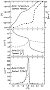 |
Fig. 16 Solution to the hydrodynamic problem for the investigation of the Hα line. |
 |
Fig. 17 Synthetic transmission spectrum of HAT-P-32 b (red) in the Hα line for the conditions of Fig. 16. Wavelengths are shifted by systemic motion of HAT-P-32. |
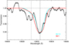 |
Fig. 18 Planetary He Iλ10833 absorption profile for the “center” phase (mid-transit, see Fig. 11) compared to two model absorption profiles for H/He ratiosof 90/10 (cyan) and 99/1 (red) (see Fig. 19) The vertical dotted lines indicate the positions of the lines. |
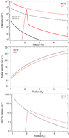 |
Fig. 19 Outputs of the He hydrodynamics model showing the H and H+ densities (top), the radial wind velocity (middle), and the He (23S) density (bottom) obtained from the fit of the observed He (23S) absorption (see Fig. 18). Profiles are shown for the canonical H/He ratio of 90/10 (black) and for a high H/He ratio of 99/1 that resembles the model of Hα (red). The temperature was 14 000 K in both cases and the mass-loss rate of 3.6 × 10¹² g s−1 and 1.6 × 10¹³ g s−1, respectively. |
8 Discussion
We analyzed two transit time series of the hot Jupiter HAT-P-32 b obtained with CARMENES and found prominent transmission signals in both the Hα and He I λ10833 lines, which we attribute to the planetary atmosphere.
8.1 Putting the transmission signals in context
None of ourresults contradicts the presence of a cloud deck, which has been suggested by several studies (Sect. 1). We speculate that the non-detection of Hα absorption by Mallonn & Strassmeier (2016) is caused by a lack of sensitivity in that study, which was not based on high-resolution spectra. However, time variability in the Hα absorption cannot be excluded as a confounding factor.
In Table 6, we list the planetary semimajor axis, mass, radius, and density along with the transmission contrasts of the Hα and He I λ10833 lines for several planets discussed in the literature in order of ascending host star effective temperature. For HAT-P-32 b the contrast is time dependent, so we report an average value derived from our phenomenological modeling presented in Sect. 6.3. To the best of our knowledge, no simultaneous detection of Hα and He I λ10833 transmission in a single planetary atmosphere has so far been reported in the literature. In HD 189733 b, however, separate detections of both lines have been published.
Among the planets in Table 6, HAT-P-32 b shows the lowest density estimate, which is, however, not exceptionally low as comparison with WASP-107 b or WASP-121 b demonstrates. In terms of reported contrast, the atmosphere of HAT-P-32 b is only second to the atmospheres of WASP-12 b and WASP-107 b in the Hα and He I λ10833 lines. While detections of He I λ10833 transmission have predominantly been found in planets orbiting stars with lower effective temperature than HAT-P-32, reports of planetary Hα transmission signals tend to be associated with planets orbiting stars with higher effective temperatures. While the photospheric NUV continua intensify toward higher effective temperatures, magnetically driven activity phenomena, such as coronal X-ray emission, are thought to vanish at about spectral type A (in main sequence stars), where the outer convection zone disappears (Teff ≈ 8000 K, e.g., Güdel 2004). It seems that the mass and effective temperature of the host star HAT-P-32 is in an intermediate region, where the mass remains sufficiently low for the star to drive a magnetic dynamo in an outer convection zone, which is thought to power the EUV emission required to populate the metastable helium level in the planetary atmosphere, and its effective temperature is high enough to foster conditions favoring the population of the H(2) ground level of Hα there.
Our results show no significant difference between the observations carried out on night 1 and night 2. This is consistent with the findings of Kirk et al. (2020) and Allart et al. (2019) in WASP-107 b and Salz et al. (2018) in HD 189733 b, who also find no detectable inter-transit variation in the He I λ10833 transmission signal. Borsa et al. (2021) report Hα line absorption in two transits of WASP-121 b with potentially variable contrast between the transits, which may be attributed to changes in the atmospheric blueshift or stellar activity levels. Yan et al. (2021a) reproduce the Hα absorption lines using one-dimensional hydrodynamic simulations with detailed radiative transfer modeling and find that different XUV irradiation levels caused by a change in the stellar activity state during the two observations are a viable explanation for the observation.
Allart et al. (2019) and Kirk et al. (2020) find evidence for blueshifted He I λ10833 absorption after the optical transit, which may be indicative of escaping material trailing WASP-107 b. Similarly, a prolonged He I λ10833 transit was found by Nortmann et al. (2018) in WASP-69 b. In HAT-P-32 b, we find no convincing evidence for post-transit absorption in the Hα or He I λ10833 lines. However, we see marked pre-transit absorption. Salz et al. (2018) report redshifted He I λ10833 line absorption during ingress in HD 189733 b, which may be caused by a super-rotating atmosphere (Lampón et al. 2021b), but no pre-transit absorption was reported. Cauley et al. (2015) and Cauley et al. (2016) report on time-variable pre- and post-transit Hα line absorption in HD 189733 b. The cause is, however, confounded by activity phenomena (Barnes et al. 2016; Cauley et al. 2017; Kohl et al. 2018).
8.2 Hydrodynamical modeling
The one-dimensional hydrodynamical models presented in Sect. 7 can reproduce the observed Hα and He I λ10833 transmission line cores during the center phase reasonably well. This refers to both the strength and width of the core transmission. We thus conclude that absorption profiles in the core are likely dominated by the radial planetary wind component of HAT-P-32 b. This result is consistent with the findings for the atmosphere of the warmNeptune GJ 3470 b (Palle et al. 2020; Lampón et al. 2021b), which also shows broadened He I λ10833 absorption.
In our Hα line modeling, the distribution of H(2) and, therefore, the Hα line opacity, is strongly concentrated within a comparatively narrow shell around the planet. This behavior is reproduced by our He I λ10833 line modeling if a high H/He ratio is assumed. A fully integrated hydrodynamical treatment of Hα and He I λ10833 line transmission was not attempted here and our hydrodynamical modeling does not, in its current form, allow the temporal variability of the transmission signal to be addressed.
Under the energy-limited escape hypothesis, a mass-loss rate of about 1013 g s−1 was predicted for HAT-P-32 b (Sect. 4.1). This rate is consistent to within a factor of a few with the values obtained from our hydrodynamical atmospheric modeling. As far as our He I λ10833 modeling is concerned, however, the solution is not unique, because the mass-loss rate is a free parameter and different model temperatures and H/He number ratios yield different best-fit estimates. While an exhaustive exploration of the parameter space and the hydrodynamic escape regime is beyond this paper (Lampón et al. 2020, 2021b,a), consistent values are obtained for plausible physical assumptions, as demonstrated in Sect. 7.
In terms of Hα absorption and modeling, it is worth comparing the cases of HAT-P-32 b and the ultra-hot Jupiter KELT-9 b, which also exhibits strong Hα absorption (Yan & Henning 2018; García Muñoz & Schneider 2019). For HAT-P-32 b, the modeling presented here shows that the H(2) layer is geometrically narrow and the outflow is principally driven by stellar irradiation in the XUV. In contrast, the H(2) layer of KELT-9 b extends significantly toward the lower atmosphere, and stellar NUV irradiation plays a key role at heating the upper atmosphere, thereby driving the outflow and producing a sizable population of H(2). Because the corresponding NUV/XUV ratios of their host star emissions differ considerably (~140 for HAT-P-32 b and ~7.5 × 10⁶ for KELT-9 b), the specifics of H(2) excitation are also different in these two (ultra-)hot Jupiters.
8.3 The shape of the atmosphere
The transmission signal of HAT-P-32 b shows a complex pattern of temporal variability with detectable pre-transit absorption in the red flank. We attempted to model the variation in the signal using a phenomenological model incorporating, first, a circumplanetary annulus, second, a super-rotating wind, and third, an up-orbit stream with velocity components directed in the orbital forward direction and toward the star (Sect. 6). The overall fit quality is best for the up-orbit stream model, followed by the super-rotating wind model and the annulus model (Table 5). As is clear from the consideration of the fit quality in the individual phases (Tables F.1 and F.2), the main differences are observed in the pre, ingress, and start phases of the transit. Both the super-rotating wind and up-orbit stream models improve the ingress-phase fit in the Hα and He I λ10833 lines with respect to the annulus atmosphere model, and the up-orbit stream model provides additional improvement over the super-rotating wind model in the He I λ10833 lines. In the start phase, the up-orbit stream model outperforms the annulus and super-rotating wind models both in the Hα and He I λ10833 lines, because neither of the latter models can produce an asymmetry in the line profile to compete with the stream model. The same holds true for the pre phase, where only the up-orbit stream model can provide an improvement. During and after the central phase, it is the annulus model, which tends to provide the best fit, although the differences are not as pronounced.
Taking the parameters of the up-orbit stream model at face value, the streaming rates of H(2) and He (23S) are about one and four times 105 g s−1. If all mass lost from the planet were transported through this stream, the average fraction of H(2) atoms in the stream would be about 10−8 and that of He atoms in the He (23S) state would be around 10−7. The numbers decrease if less mass is funneled through the stream and they depend on the composition. By comparison with our hydrodynamic models, we find that a fraction of H(2) of 10−8 corresponds to that found at about two planetary radii. Likewise, the radius corresponding to a He(23S) fraction of 10−7 is found at six planetary radii (H/He 90/10). While a detailed hydrodynamic modeling is clearly required to understand the physical regime, this demonstrates that the order of magnitude of these numbers are not at odds with those of the outer planetary atmosphere.As the circumplanetary environment around HAT-P-32 b is complex, further atmospheric components, such as a circumplanetary disk, may be present, which have not been accounted for in our phenomenological modeling so far.
Compilation (possibly incomplete) of Hα and He I λ10833 transmission line contrasts, listed in order of ascending effective host star temperature.
9 Conclusion
HAT-P-32 is a highly active F-type star with an X-ray luminosity of 2.3 × 1029 erg s−1 (5–100 Å band) as measured by XMM-Newton. The star is orbited by the low-density planet HAT-P-32 b on an oblique, circular orbit. Energy-limited escape considerations lead to an estimate on the order of 1013 g s−1 for the mass-loss rate.
Our CARMENES high-resolution optical and NIR transmission spectra show pronounced absorption signals in the Hα and He I λ10833 triplet lines, which we attribute to the planetary atmosphere. To the best of our knowledge, HAT-P-32 b is the first exoplanet in which both Hα and He I λ10833 signals could simultaneously be detected and both absorption signals are among the strongest yet observed in planetary atmospheres. The transmission signals are time dependent. In particular, an early ingress of redshifted absorption is observed in both lines, though more clearly in the He I λ10833 triplet lines. We used phenomenological transmission models to demonstrate that this signal is plausibly caused by an up-orbit stream. Such a component is in agreement with predictions of hydrodynamical models by of comparable systems Lai et al. (2010); Bisikalo et al. (2013); Carroll-Nellenback et al. (2017), and the configuration resembles the type III star-planet interaction scenario described by Matsakos et al. (2015).
Among the sample of planets with known atmospheric Hα or He I λ10833 absorption signals, HAT-P-32 b is situated on the low end of the density range (Table 6). While detections of Hα absorption have predominantly been reported in systems with host stars of higher effective temperature, those of He I λ10833 absorption tend to be associated with systems with cooler host stars. Although the number of systems remains low, the presumed dichotomy in the distribution of Hα and He I λ10833 signals can plausibly be attributed the evolution of magnetic activity and NUV photospheric continua as a function of spectral type.
Hydrodynamic one-dimensional models of the mid-transit absorption signals of the Hα and He I λ10833 lines presented in this paper reproduce the observed line profiles well, indicating that the absorption in the line cores is explained by a radial planetary wind. The mass-loss rates predicted by the hydrodynamic models are consistent with 1013 g s−1 to within factors of a few, which is in line with predictions from energy-limited escape. The assumption of a constant mass-loss rate yields a lifetime of about 3.5 Gyr for HAT-P-32 b, comparable to the estimated system age of 2.7 ± 0.8 Gyr (Hartman et al. 2011). Clearly, this makes hydrodynamic escape a key factor for the planetary evolution of HAT-P-32 b, which may have started out with about twice its current mass. In terms of host star activity and system geometry, HAT-P-32 b is one of the most peculiar systems observed to date, making HAT-P-32 a testbed for our understanding of planetary mass-loss and evolution.
Acknowledgements
We thank Norbert Schartel for providing XMM-Newton DDT time. We thank M. Salz, F. Bauer, and F. J. Alonso-Floriano for highly valuable contributions to this paper. CARMENES is an instrument for the Centro Astronómico Hispano-Alemán (CAHA) at Calar Alto (Almería, Spain), operated jointly by the Junta de Andalucía and the Instituto de Astrofísica de Andalucía (CSIC). CARMENES was funded by the Max-Planck-Gesellschaft (MPG), the Consejo Superior de Investigaciones Científicas (CSIC), the Ministerio de Economía y Competitividad (MINECO) and the European Regional Development Fund (ERDF) through projects FICTS-2011-02, ICTS-2017-07-CAHA-4, and CAHA16-CE-3978, and the members of the CARMENES Consortium (Max-Planck-Institut für Astronomie, Instituto de Astrofísica de Andalucía, Landessternwarte Königstuhl, Institut de Ciències de l’Espai, Institut für Astrophysik Göttingen, Universidad Complutense de Madrid, Thüringer Landessternwarte Tautenburg, Instituto de Astrofísica de Canarias, Hamburger Sternwarte, Centro de Astrobiología and Centro Astronómico Hispano-Alemán), with additional contributions by the MINECO, the Deutsche Forschungsgemeinschaft through the Major Research Instrumentation Programme and Research Unit FOR2544 “Blue Planets around Red Stars”, the Klaus Tschira Stiftung, the states of Baden-Württemberg and Niedersachsen, and by the Junta de Andalucía. Based on data from the CARMENES data archive at CAB (CSIC-INTA). We acknowledge financial support from the Agencia Estatal de Investigación of the Ministerio de Ciencia, Innovación y Universidades and the ERDF through projects PID2019-109522GB-C5[1:4]/AEI/10.13039/501100011033 PGC2018-098153-B-C33 and the Centre of Excellence “Severo Ochoa” and “María de Maeztu” awards to the Instituto de Astrofísica de Canarias (SEV-2015-0548), Instituto de Astrofísica de Andalucía (SEV-2017-0709), and Centro de Astrobiología (MDM-2017-0737), the Generalitat de Catalunya/CERCA programme. D. Yan acknowledges support by the Strategic Priority Research Program of Chinese Academy of Sciences, Grant No. XDB 41000000 and National Natural Science Foundation of China (Nos. 11973082). SC and EN acknowledge DFG support under grants CZ 222/3-1 and CZ 222/5-1. This research has made use of the Exoplanet Orbit Database and the Exoplanet Data Explorer at exoplanets.org. This work has made use of data from the European Space Agency (ESA) mission Gaia (https://www.cosmos.esa.int/gaia), processed by the Gaia Data Processing and Analysis Consortium (DPAC, https://www.cosmos.esa.int/web/gaia/dpac/consortium). Funding for the DPAC has been provided by national institutions, in particular the institutions participating in the Gaia Multilateral Agreement.
Appendix A Observing log
Tables A.1 and A.2 give the observational logs for nights 1 and 2.
Observational log for night 1.
Observational log for night 2.
Appendix B Telluric correction
The spectralregions of the optical Hα and infrared He Iλ10833 triplet lines are affected by water absorption lines. The infrared is additionally contaminated by OH emission lines. All of these must be corrected to obtain reliable results from transmission spectroscopy.
B.1 Absorption lines
The telluric transmission spectrum in the region of the He I λ10833 lines is dominated by water absorption lines. In Fig. B.1, we plot as an example the first spectrum obtained on night 1 along with atelluric transmission model obtained with molecfit. The locations of the most relevant water absorption lines at 10 829.69, 10833.32, 10 834.59, 10 835.07, 10 836.94, 10 837.12 Å are indicated (see also Kleiber & Zeileis 2008; Gordon et al. 2017, for the line data bases).
We fitted the depth of the atmospheric water vapor column using several parts of the observed spectrum using molecfit. Stellar lines are not a serious interference in the NIR in HAT-P-32, because they are sparse and broad. We then obtained the model telluric transmission spectrum using molecfit and divided by it to correct for the water vapor contamination. In Fig. B.2, we show our results for the depth of the atmospheric water vapor column as afunction of time. Clearly, the first night is more heavily affected by telluric water absorption than the second. In both nights, the depth of the water column remains rather stable during the respective observing run.
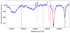 |
Fig. B.1 Excerpt of the first spectrum on night 1 (blue dots) along with telluric absorption model (solid red) and locations of relevant water absorption lines (vertical dashed black). Hydroxide emission lines are indicated by shorter, dotted red lines. |
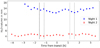 |
Fig. B.2 The depth of the water column obtained with molecfit by fitting the NIR channel data as a function of time. |
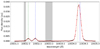 |
Fig. B.3 Mean sky spectrum during night 1 (black points) along with best-fit model (solid red line) and wavelengths of the Q1 and Q2 doublet lines according to Oliva et al. (2015) (f-components green dotted, e-components dashed blue vertical lines). Gray-shaded regions are exempted from the fit. |
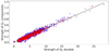 |
Fig. B.4 Ratio between strengths of the Gaussian model components representing the Q2 e (blue stars) and Q2f (red pluses) lines and the strength of the combined Q1 components along with best-fit relation (dashed black). |
Telluric emission lines of OH with line identifications as specified by Oliva et al. (2015).
B.2 Emission lines
In the vicinity of the He Iλ10833 lines, four emission lines of hydroxide (OH) are prominent (Oliva et al. 2015), the vacuum wavelengths and identifications of which are reproduced in Table B.1. We here use the same nomenclature for line identification as Phillips et al. (2004). In the table, the lines are arranged in two rows, each representing the lines of a so-called Λ-doublet, resulting from spin–orbit coupling. Their components are designated by letters e and f, indicating lower state parity. All lines considered here derive from a transition between vibrational states with quantum numbers five and two. Both doublets belong to the Q-branch, where transitions do not involve a change in the rotational quantum number. The Q-subscript indicates the spin quantum number and the second number in parenthesis the orbital angular momentum, pertaining to both the upper and lower state. In Fig. B.3, we show the mean sky spectrum observed by the sky-fiber during the night 1 run along with the line locations listed in Table B.1. While the Q2 doublet is easily resolved by CARMENES, the Q1 doublet is not.
B.2.1 Emission line behavior
To produce a correction scheme for the sky emission lines, we studied the strength and evolution of the three resolved OH components using a total of 1836 CARMENES sky-fiber spectra obtained in the context of our two observing runs and several other observing runs obtained by the CARMENES consortium. To model the sky emission spectrum around the He I λ10833 triplet lines, we used a model consisting of three Gaussian components and an offset parameter, which was fitted to all individual sky-emission spectra. In the fit, we vary the areas of the three Gaussians independently and adapt the offset parameter. While we assumed the instrumental width for the resolved lines of the Q2 doublet, the width of the component representing the blended Q1 doublet was left as a free parameter. We also allowed for a small shift in the line wavelengths. Although the CARMENES pipeline (Zechmeister et al. 2018) is excellent in dealing with detector defects, we chose to mask the two gray-shaded spectral regions indicated in Fig. B.3 in the fit because they can be affected by known bad pixels. As an example, we also show the best-fit model to the mean night 1 sky spectrum in Fig. B.3.
In Fig. B.4, we show the fitted strengths of the individual Q2 emission lines as a function of that of the Q1 line components. Prior to the analysis, a small number of 13 outliers were rejected based on the Generalized Extreme Studentized Deviate (ESD) test (Rosner 1983). The e and f components of the doublets arise from spin–orbit coupling. They should therefore behave essentially identically, which is consistent with our findings. The two considered λ-doublets also arise from closely related transitions and are therefore expected to behave similarly. Our results are consistent with a linear relation between the strength of the Q1 doublet and the Q2 doublet components. Thus, we obtained the best-fit ratio by regression through the origin. The resulting ratio,
 (B.1)
(B.1)
is also shown in Fig. B.4. The uncertainty was derived using the Jackknife method (Efron & Stein 1981). The strength of the combined Q1 doublet lines is larger than its Q2 equivalent by about an order of magnitude, which is consistent with the results obtained by Oliva et al. (2015).
Similar ratios between OH emission lines can be used to study the conditions of the upper atmosphere (Phillips et al. 2004). However, the ratio derived above is biased with respect to the physical value because the spectral sampling is not taken into account in the modeling. The ratio is appropriate in the correction of our science spectra, because they were treated identically.
B.2.2 Emission line correction
To correct the emission line contribution in the science spectra, we made use of the modeling in Sect. B.2.1. The unresolved Q1 doublet lines are prominent also in the science spectra (Fig. B.1). As HAT-P-32 is a fast rotator, the strength of the comparatively narrow Q1 doublet can be determined by a Gaussian fit with relative ease also in the science spectra. Based on this value and the now known relation between the strengths of the Q1 and weaker Q2 components, we constructed a model emission spectrum based on the Gaussian modeling and subtract it from the science spectrum.
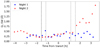 |
Fig. B.5 Equivalent width of the Q1 doublet as afunction of time. |
The resulting EW of the Q1 component during nights 1 and 2 is shown in Fig. B.5. Until about fourth contact, the OH contamination of the spectra is relatively similar on nights 1 and 2. After the transit on night 2, the EW of OH emission rises and has approximately tripled at the end of the observing run compared to its start. In Fig. B.6, we show the effect of the removal of a telluric emission lines using the most heavily contaminated spectrum, viz., the last spectrum of night 2, as an example. This figure also displays an example for the removal a telluric water absorption line at 10 835.07 Å. Although the emission lines are very prominent in the spectrum, the correction reduces them substantially. Nonetheless, some residuals remain (e.g., Sect. 5.5).
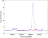 |
Fig. B.6 Excerpt of normalized last spectrum from night 2 before (blue, dotted) and after (red, dashed) correction for OH emission lines. The correction for telluric absorption lines is also included. |
Appendix C Reference spectra
To study the presence of an additional absorption component superimposed on the stellar spectrum during transit, a reference spectrum representing the stellar spectrum, Fr, needs to be known as accurately as possible for comparison. As the stellar spectrum may be variable, for example, because of stellar activity (e.g., Klocová et al. 2017) and the observed spectrum is affected by variable telluric contamination, spectra obtained near the transit event under consideration were preferred for the construction of such a reference. The combination of several spectra increases the S/N of the reference. Incorporation of spectra obtained prior and past the time range is often desirable to diagnose spectral changes and potentially counterbalance small changes in the observed spectrum evolving linearly in time.
In the following,  denotes a suitable subset of theobserved spectra and fi(λ) refers to thenormalized flux density after the barycentric velocity correction, the telluric correction, and possible further pertinent treatment. We proceeded to construct a reference spectrum by averaging the resulting spectral flux density
 (C.1)
(C.1)
where  is the number of spectra in the set. If the RV shift of the star is relevant across the subset
  or considerable changes in the S/N take place, such effects may also have to be taken into account, but we consider this unnecessary here.
C.1 Reference spectrum for night 1
On night 1, a suitable reference spectrum could be constructed by averaging the spectra with numbers 1 − 3 and 20 − 23 as defined in Table A.1, which cover the exposures obtained about 2.2 h or more before and after the transit. This choice incorporates pre- and post-transit coverage and uses spectra comfortably set apart in time from the actual optical transit. In Fig. C.1, we show the reference spectra in the spectral region around the Hα and He I λ10833 lines separately for the indicated ranges of pre- and post-transit spectra. Additionally, we show their ratio and estimated 95 % confidence range of variation resulting from noise. Naturally, the core of the deep Hα line suffers from an elevated noise level caused by the flux depression. We found the two ratios to be consistent within the expected noise variation. Therefore, we used the combined spectra as final reference spectra ( ).
).
C.2 Reference spectrum for night 2
On night 2 we have more pre- and post-transit coverage in our data set. Unfortunately, the post-transit NIR data suffer from two deteriorating and likely related effects, viz., a decrease in S/N in the stellar spectrum, accompanied by a strengthening of telluric emission compared to the stellar signal. This is not the case for the VIS data.
Combining the spectra with the log numbers 1 − 6 for the pre-transit and 24 − 28 for the post-transit reference fulfills about the same timing requirements as used on night 1, each range being offset by more than 2.2 h from the actual optical transit center. In Fig. C.2, we again show the resulting reference spectra along with their ratio around the Hα and the He I λ10833 lines. The situation around the Hα line is satisfactory. Around the He Iλ10833 lines, we found a less satisfying situation. The effect of the lower S/N obtained post-transit was clearly reflected by larger scatter in the associated reference spectrum. The ratio of the pre- and post-transit spectra shows systematic deviations certainly related to the telluric emission lines and perhaps other effects. We note that the emission line corresponding to the Q1 doublet reaches a peak height of around 6.5 in the post-transit reference compared to about 2.5 in the pre-transit reference. It appears that the line develops non-Gaussian wings, which were not corrected atthe required level. Also, the Si I line shows deviations of unknown origin. As neither the Hα line shown in Fig. C.2 nor the Ca II IRT lines provide evidence for significant variation related to activity, we decided to only use the pre-transit reference for the spectral region around the He I λ10833 lines, while the pre- and post-transit spectra can be used for the Hα line, in particular,  and 𝒮r,n2,VIS = {1,2,3,4,5,6,24,25,26,27,28}.
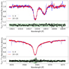 |
Fig. C.1 Comparison of pre- and post-transit reference spectra. Top plot, top panel: Averaged, normalized pre-transit spectra (nos. 1,2,3) and post-transit spectra (nos. 20 − 23) around the He Iλ10833 lines during night 1. Dotted lines indicate the averaged spectra obtained without our telluric emission line correction. Top plot, bottom panel shows the ratio of the averaged post- and pre-transit spectra along with an estimate of the 95 % confidencerange resulting from noise (green shades). The bottom panels show the same for the Hα line region. |
Appendix D Treatment of phase smearing
When g(x) is a continuous distribution function with variance  and mean μg then
 (D.1)
(D.1)
Here, we take g(x) to describe the profile of an instrumentally broadened spectral line. A new distribution, f(x), is generated by shifting the original distribution between  and
and  around its mean (i.e., by convolution with a box-like profile) so that
 (D.2)
(D.2)
This is equivalent to a convolution with a box-shaped profile. Symmetry implies identical mean values μg = μf. The variance of f(x) is given by

The additional, second variance term can be absorbed in the instrumental resolution.
CARMENES provides a spectral resolution of 80 400, which corresponds to a line profile with full-width at half-maximum (FWHM) of 3.7 km s−1 in the NIR arm. For Gaussian profiles, the FWHM and the standard deviation, which is the square root of the variance, are related by a factor of  . In the case of HAT-P-32 b, phase smearing adds another 2.3 km2 s−2 to the variance. The effective resolution, including phase smearing, becomes 58 000. In the optical arm, an effective resolution of 63 000 applies.
Appendix E Uncertainty of transmission spectra
To estimate the uncertainty of the data points in the combined transmission spectra from night 1 and night 2, we used the βσ estimator as given by Czesla et al. (2018).
Standard deviation, σ, of uncertainty for individual data points (in units of 10−2).
The transmission spectra are oversampled so that consecutive data points are not independent. We find a mean autocorrelation scale, τa, of 11 data points in the transmission spectra. Using a “jump parameter” of 22 data points samples independent points to estimate the noise. Combined with a second-order approximation of the underlying variation, we obtain the standard deviations, σ, for the transmission spectra obtained for the Hα and He I λ10833 lines in the individual phases. In estimating χ2 and BIC values, we use an effective number of independent data points given by
 (E.1)
(E.1)
where N is the number of points in the oversampled transmission spectrum (Bayley & Hammersley 1946; Priestley 1981).
Appendix F Fit quality in phenomenological modeling
Fit results of phenomenological modeling ((−100, +100) km s−1 region). χ2 and reduced χ2 values for annulus (a), super-rotating wind model (w), and up-orbit stream model (s).
Values of Bayesian information criterion for comparison of annulus model (a), super-rotating wind model (w), and up-orbit stream model (s). Negative values indicate preference for the first-mentioned model.
Appendix G Exchanging convolution and exponentiation
If g(λ;λ0, σ2) denotes the normal density withmean λ0 and variance σ2, we observe that for positive integer n
 (G.1)
(G.1)
where
 (G.2)
(G.2)
For positive, real x, the exponential function can be expanded into
 (G.3)
(G.3)
If the instrumental profile, R, is normal such that R =  and the optical depth profile, τ(λ), is proportional to a normal density such that
 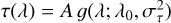 . This implies that the optical depth at the line center, dτ, is
  . The optical depth profile, τ(λ), leads to an observed spectral line of the form s(λ) = R * exp(−τ(λ)), where * denotes the convolution. As the result of the convolution of two normal functions is conveniently also normal, the question as to when it is appropriate to absorb the instrumental profile in the optical depth arises. To that end, we investigate the difference
 (G.4)
(G.4)
Combining Eqs. G.1 and Eq. G.3, one obtains
 (G.5)
(G.5)
The first two terms (constant and linear) in the expansion cancel and, therefore,
![Mathematical equation: \begin{eqnarray*}\delta(\lambda) &=& \sum_{n=2}^{\infty} \frac{(-1){}^n\,A^n}{n!} \left[c_n(\sigma_{\tau}^2) g\left(\lambda_0,\frac{\sigma_{\tau}^2}{n}+\sigma_R^2\right) \right. - \nonumber \\& & \left. c_n(\sigma_R^2+\sigma_{\tau}^2) g\left(\lambda_0,\frac{\sigma_{\tau}^2+\sigma_R^2}{n}\right) \right] \;.\end{eqnarray*}](/articles/aa/full_html/2022/01/aa39919-20/aa39919-20-eq49.png) (G.6)
(G.6)
Focusing on the line center, and defining  with α > 0, we find
![Mathematical equation: \begin{eqnarray*}\delta(\lambda_0) &=& \sum_{n=2}^{\infty} \frac{(-1){}^n\,A^n}{n!} \left[c_n(\sigma_{\tau}^2) \left(2\pi\left(\frac{\sigma_{\tau}^2}{n}+\sigma_R^2\right) \right){}^{-\frac{1}{2}} \right. - \nonumber \\& & \left. c_n(\sigma_R^2+\sigma_{\tau}^2) \left(2\pi \left(\frac{\sigma_{\tau}^2+\sigma_R^2}{n}\right)\right){}^{-\frac{1}{2}} \right] \; \nonumber \\&=& \sum_{n=2}^{\infty} \left(\frac{A}{\sqrt{2\pi\sigma_{\tau}^2}}\right){}^n \frac{(-1){}^n}{n!} \left(\frac{1}{\sqrt{(1+n\alpha)}} - \frac{1}{(1+\alpha){}^{\frac{n}{2}}} \right) \nonumber \\&=& \sum_{n=2}^{\infty} d_{\tau}^n \, \frac{(-1){}^n}{n!} \left(\frac{1}{\sqrt{(1+n\alpha)}} - \frac{1}{(1+\alpha){}^{\frac{n}{2}}} \right)\;. \end{eqnarray*}](/articles/aa/full_html/2022/01/aa39919-20/aa39919-20-eq51.png) (G.7)
(G.7)
The sum in Eq. G.7 consists of terms with alternating sign, as the term in parentheses is always positive. The sum converges by construction. Although the summands tend to decrease quickly in absolute value, owing to the inverse dependence on the factorial of n, monotonous decrease, which is required for convergence, does not necessarily set in immediately. Nonetheless, a good approximation can usually be obtained, considering only a few leading summands.
In the case of dτ = 1 and α = 0.1, which is typical of values encountered in this paper, the difference δ(λ0) is about 10−3.
References
- Albrecht, S., Winn, J. N., Johnson, J. A., et al. 2012, ApJ, 757, 18 [NASA ADS] [CrossRef] [Google Scholar]
- Allart, R., Bourrier, V., Lovis, C., et al. 2018, Science, 362, 1384 [Google Scholar]
- Allart, R., Bourrier, V., Lovis, C., et al. 2019, A&A, 623, A58 [NASA ADS] [CrossRef] [EDP Sciences] [Google Scholar]
- Alonso-Floriano, F. J., Sánchez-López, A., Snellen, I. A. G., et al. 2019a, A&A, 621, A74 [NASA ADS] [CrossRef] [EDP Sciences] [Google Scholar]
- Alonso-Floriano, F. J., Snellen, I. A. G., Czesla, S., et al. 2019b, A&A, 629, A110 [NASA ADS] [CrossRef] [EDP Sciences] [Google Scholar]
- Barnes, J. R., Haswell, C. A., Staab, D., & Anglada-Escudé, G. 2016, MNRAS, 462, 1012 [Google Scholar]
- Bayley, G. V., & Hammersley, J. M. 1946, Suppl. J. R. Stat. Soc., 8, 184 [CrossRef] [Google Scholar]
- Bisikalo, D., Kaygorodov, P., Ionov, D., et al. 2013, ApJ, 764, 19 [NASA ADS] [CrossRef] [Google Scholar]
- Borsa, F., Allart, R., Casasayas-Barris, N., et al. 2021, A&A, 645, A24 [EDP Sciences] [Google Scholar]
- Brogi, M., Giacobbe, P., Guilluy, G., et al. 2018, A&A, 615, A16 [NASA ADS] [CrossRef] [EDP Sciences] [Google Scholar]
- Caballero, J. A., Guàrdia, J., López del Fresno, M., et al. 2016, in SPIE Conf. Ser., 9910, Proc. SPIE, 99100E [Google Scholar]
- Cabot, S. H. C., Madhusudhan, N., Welbanks, L., Piette, A., & Gandhi, S. 2020, MNRAS, 494, 363 [Google Scholar]
- Carroll-Nellenback, J., Frank, A., Liu, B., et al. 2017, MNRAS, 466, 2458 [NASA ADS] [CrossRef] [Google Scholar]
- Casasayas-Barris, N., Palle, E., Nowak, G., et al. 2017, A&A, 608, A135 [NASA ADS] [CrossRef] [EDP Sciences] [Google Scholar]
- Casasayas-Barris, N., Pallé, E., Yan, F., et al. 2018, A&A, 616, A151 [NASA ADS] [CrossRef] [EDP Sciences] [Google Scholar]
- Casasayas-Barris, N., Pallé, E., Yan, F., et al. 2019, A&A, 628, A9 [NASA ADS] [CrossRef] [EDP Sciences] [Google Scholar]
- Casasayas-Barris, N., Pallé, E., Yan, F., et al. 2020, A&A, 635, A206 [NASA ADS] [CrossRef] [EDP Sciences] [Google Scholar]
- Castelli, F., & Kurucz, R. L. 2003, in IAU Symposium, 210, Modelling of Stellar Atmospheres, eds. N. Piskunov, W. W. Weiss, & D. F. Gray, A20 [NASA ADS] [Google Scholar]
- Cauley, P. W., Redfield, S., Jensen, A. G., et al. 2015, ApJ, 810, 13 [NASA ADS] [CrossRef] [Google Scholar]
- Cauley, P. W., Redfield, S., Jensen, A. G., & Barman, T. 2016, AJ, 152, 20 [NASA ADS] [CrossRef] [Google Scholar]
- Cauley, P. W., Redfield, S., & Jensen, A. G. 2017, AJ, 153, 217 [NASA ADS] [CrossRef] [Google Scholar]
- Cauley, P. W., Shkolnik, E. L., Ilyin, I., et al. 2019, AJ, 157, 69 [Google Scholar]
- Cauley, P. W., Wang, J., Shkolnik, E. L., et al. 2021, AJ, 161, 152 [Google Scholar]
- Chen, G., Casasayas-Barris, N., Pallé, E., et al. 2020, A&A, 635, A171 [NASA ADS] [CrossRef] [EDP Sciences] [Google Scholar]
- Czesla, S., Klocová, T., Khalafinejad, S., Wolter, U., & Schmitt, J. H. M. M. 2015, A&A, 582, A51 [NASA ADS] [CrossRef] [EDP Sciences] [Google Scholar]
- Czesla, S., Molle, T., & Schmitt, J. H. M. M. 2018, A&A, 609, A39 [NASA ADS] [CrossRef] [EDP Sciences] [Google Scholar]
- Czesla, S., Schröter, S., Schneider, C. P., et al. 2019, PyA: Python astronomy-related packages [Google Scholar]
- Daley-Yates, S., & Stevens, I. R. 2019, MNRAS, 483, 2600 [NASA ADS] [CrossRef] [Google Scholar]
- Damiano, M., Morello, G., Tsiaras, A., Zingales, T., & Tinetti, G. 2017, AJ, 154, 39 [NASA ADS] [CrossRef] [Google Scholar]
- Deming, D., & Sheppard, K. 2017, ApJ, 841, L3 [NASA ADS] [CrossRef] [Google Scholar]
- Drake, G. 2006, High Precision Calculations for Helium, ed. G. Drake (New York, NY: Springer New York), 199 [Google Scholar]
- Efron, B., & Stein, C. 1981, Ann. Stat., 9, 586 [CrossRef] [Google Scholar]
- Eggleton, P. P. 1983, ApJ, 268, 368 [Google Scholar]
- Ehrenreich, D., Bourrier, V., Wheatley, P. J., et al. 2015, Nature, 522, 459 [Google Scholar]
- Erkaev, N. V., Kulikov, Y. N., Lammer, H., et al. 2007, A&A, 472, 329 [NASA ADS] [CrossRef] [EDP Sciences] [Google Scholar]
- Fuhrmeister, B., Czesla, S., Schmitt, J. H. M. M., et al. 2018, A&A, 615, A14 [NASA ADS] [CrossRef] [EDP Sciences] [Google Scholar]
- Fuhrmeister, B., Czesla, S., Hildebrandt, L., et al. 2019, A&A, 632, A24 [NASA ADS] [CrossRef] [EDP Sciences] [Google Scholar]
- Fuhrmeister, B., Czesla, S., Hildebrandt, L., et al. 2020, A&A, 640, A52 [NASA ADS] [CrossRef] [EDP Sciences] [Google Scholar]
- Fulton, B. J., & Petigura, E. A. 2018, AJ, 156, 264 [Google Scholar]
- Fulton, B. J., Petigura, E. A., Howard, A. W., et al. 2017, AJ, 154, 109 [Google Scholar]
- Gaia Collaboration (Brown, A. G. A., et al.) 2018, A&A, 616, A1 [NASA ADS] [CrossRef] [EDP Sciences] [Google Scholar]
- García Muñoz, A. 2007, Planet. Space Sci., 55, 1426 [Google Scholar]
- García Muñoz, A., & Schneider, P. C. 2019, ApJ, 884, L43 [Google Scholar]
- Gibson, N. P., Aigrain, S., Barstow, J. K., et al. 2013, MNRAS, 436, 2974 [CrossRef] [Google Scholar]
- Gordon, I., Rothman, L., Hill, C., et al. 2017, J. Quant. Spectr. Rad. Transf., 130, 4 [NASA ADS] [Google Scholar]
- Gray, R. O., & Corbally, C. J. 1994, AJ, 107, 742 [Google Scholar]
- Güdel, M. 2004, A&ARv, 12, 71 [CrossRef] [Google Scholar]
- Guilluy, G., Andretta, V., Borsa, F., et al. 2020, A&A, 639, A49 [EDP Sciences] [Google Scholar]
- Han, E., Wang, S. X., Wright, J. T., et al. 2014, PASP, 126, 827 [NASA ADS] [CrossRef] [Google Scholar]
- Hartman, J. D., Bakos, G. Á., Torres, G., et al. 2011, ApJ, 742, 59 [NASA ADS] [CrossRef] [Google Scholar]
- Hilditch, R. W. 2001, An Introduction to Close Binary Stars, 392 [Google Scholar]
- Husser, T.-O., Wende-von Berg, S., Dreizler, S., et al. 2013, A&A, 553, A6 [NASA ADS] [CrossRef] [EDP Sciences] [Google Scholar]
- Jansen, F., Lumb, D., Altieri, B., et al. 2001, A&A, 365, L1 [NASA ADS] [CrossRef] [EDP Sciences] [Google Scholar]
- Jensen, A. G., Redfield, S., Endl, M., et al. 2012, ApJ, 751, 86 [Google Scholar]
- Jensen, A. G., Cauley, P. W., Redfield, S., Cochran, W. D., & Endl, M. 2018, AJ, 156, 154 [Google Scholar]
- Kasper, D., Bean, J. L., Oklopčić, A., et al. 2020, AJ, 160, 258 [Google Scholar]
- Kausch, W., Noll, S., Smette, A., et al. 2015, A&A, 576, A78 [NASA ADS] [CrossRef] [EDP Sciences] [Google Scholar]
- Khalafinejad, S., von Essen, C., Hoeijmakers, H. J., et al. 2017, A&A, 598, A131 [NASA ADS] [CrossRef] [EDP Sciences] [Google Scholar]
- Kirk, J., Alam, M. K., López-Morales, M., & Zeng, L. 2020, AJ, 159, 115 [Google Scholar]
- Kleiber, C., & Zeileis, A. 2008, Applied Econometrics with R (New York: Springer-Verlag) [CrossRef] [Google Scholar]
- Klocová, T., Czesla, S., Khalafinejad, S., Wolter, U., & Schmitt, J. H. M. M. 2017, A&A, 607, A66 [NASA ADS] [CrossRef] [EDP Sciences] [Google Scholar]
- Knutson, H. A., Charbonneau, D., Allen, L. E., et al. 2007, Nature, 447, 183 [NASA ADS] [CrossRef] [Google Scholar]
- Knutson, H. A., Fulton, B. J., Montet, B. T., et al. 2014, ApJ, 785, 126 [NASA ADS] [CrossRef] [Google Scholar]
- Kohl, S., Salz, M., Czesla, S., & Schmitt, J. H. M. M. 2018, A&A, 619, A96 [NASA ADS] [CrossRef] [EDP Sciences] [Google Scholar]
- Lafarga, M., Ribas, I., Lovis, C., et al. 2020, A&A, 636, A36 [NASA ADS] [CrossRef] [EDP Sciences] [Google Scholar]
- Lai, D., Helling, C., & van den Heuvel, E. P. J. 2010, ApJ, 721, 923 [NASA ADS] [CrossRef] [Google Scholar]
- Lampón, M., López-Puertas, M., Lara, L. M., et al. 2020, A&A, 636, A13 [NASA ADS] [CrossRef] [EDP Sciences] [Google Scholar]
- Lampón, M., López-Puertas, M., Czesla, S., et al. 2021a, A&A, 648, L7 [NASA ADS] [CrossRef] [EDP Sciences] [Google Scholar]
- Lampón, M., López-Puertas, M., Sanz-Forcada, J., et al. 2021b, A&A, 647, A129 [EDP Sciences] [Google Scholar]
- Latham, D. W. 1996, in Astronomical Society of the Pacific Conference Series, 90, The Origins, Evolution, and Destinies of Binary Stars in Clusters, eds. E. F. Milone, & J. C. Mermilliod, 31 [Google Scholar]
- Lecavelier des Etangs, A., Ehrenreich, D., Vidal-Madjar, A., et al. 2010, A&A, 514, A72 [NASA ADS] [CrossRef] [EDP Sciences] [Google Scholar]
- Li, S.-L., Miller, N., Lin, D. N. C., & Fortney, J. J. 2010, Nature, 463, 1054 [NASA ADS] [CrossRef] [Google Scholar]
- Louden, T., & Wheatley, P. J. 2015, ApJ, 814, L24 [CrossRef] [Google Scholar]
- Lubow, S. H., & Shu, F. H. 1975, ApJ, 198, 383 [NASA ADS] [CrossRef] [Google Scholar]
- Mallonn, M., & Strassmeier, K. G. 2016, A&A, 590, A100 [NASA ADS] [CrossRef] [EDP Sciences] [Google Scholar]
- Mallonn, M., & Wakeford, H. R. 2017, Astron. Nachr., 338, 773 [NASA ADS] [CrossRef] [Google Scholar]
- Mallonn, M., Bernt, I., Herrero, E., et al. 2016, MNRAS, 463, 604 [NASA ADS] [CrossRef] [Google Scholar]
- Mallonn, M., Köhler, J., Alexoudi, X., et al. 2019, A&A, 624, A62 [NASA ADS] [CrossRef] [EDP Sciences] [Google Scholar]
- Martin, J., Fuhrmeister, B., Mittag, M., et al. 2017, A&A, 605, A113 [NASA ADS] [CrossRef] [EDP Sciences] [Google Scholar]
- Matsakos, T., Uribe, A., & Königl, A. 2015, A&A, 578, A6 [NASA ADS] [CrossRef] [EDP Sciences] [Google Scholar]
- McCann, J., Murray-Clay, R. A., Kratter, K., & Krumholz, M. R. 2019, ApJ, 873, 89 [NASA ADS] [CrossRef] [Google Scholar]
- Nikolov, N., Sing, D. K., Goyal, J., et al. 2018, MNRAS, 474, 1705 [NASA ADS] [CrossRef] [Google Scholar]
- Ninan, J. P., Stefansson, G., Mahadevan, S., et al. 2020, ApJ, 894, 97 [Google Scholar]
- Nortmann, L., Pallé, E., Murgas, F., et al. 2016, A&A, 594, A65 [NASA ADS] [CrossRef] [EDP Sciences] [Google Scholar]
- Nortmann, L., Pallé, E., Salz, M., et al. 2018, Science, 362, 1388 [Google Scholar]
- Oliva, E., Origlia, L., Scuderi, S., et al. 2015, A&A, 581, A47 [NASA ADS] [CrossRef] [EDP Sciences] [Google Scholar]
- Palle, E., Nortmann, L., Casasayas-Barris, N., et al. 2020, A&A, 638, A61 [EDP Sciences] [Google Scholar]
- Paragas, K., Vissapragada, S., Knutson, H. A., et al. 2021, ApJ, 909, L10 [NASA ADS] [CrossRef] [Google Scholar]
- Parker, E. N. 1958, ApJ, 128, 664 [Google Scholar]
- Phillips, F., B. Burns, G., J. R. French, W., et al. 2004, Ann. Geophys., 22 [Google Scholar]
- Pino, L., Ehrenreich, D., Wyttenbach, A., et al. 2018, A&A, 612, A53 [NASA ADS] [CrossRef] [EDP Sciences] [Google Scholar]
- Pizzolato, N., Maggio, A., Micela, G., Sciortino, S., & Ventura, P. 2003, A&A, 397, 147 [NASA ADS] [CrossRef] [EDP Sciences] [Google Scholar]
- Priestley, M. 1981, Spectral Analysis and Time Series, Probability and mathematical statistics: a series of monographs and texbooks, 1–2 (Academic Press) [Google Scholar]
- Quirrenbach, A., Amado, P., Ribas, I., et al. 2018, Proc. SPIE, 10702 [Google Scholar]
- Redfield, S., Endl, M., Cochran, W. D., & Koesterke, L. 2008, ApJ, 673, L87 [Google Scholar]
- Ridden-Harper, A. R., Snellen, I. A. G., Keller, C. U., et al. 2016, A&A, 593, A129 [NASA ADS] [CrossRef] [EDP Sciences] [Google Scholar]
- Rosner, B. 1983, Technometrics, 25, 165 [Google Scholar]
- Salz, M., Czesla, S., Schneider, P. C., & Schmitt, J. H. M. M. 2016a, A&A, 586, A75 [NASA ADS] [CrossRef] [EDP Sciences] [Google Scholar]
- Salz, M., Schneider, P. C., Czesla, S., & Schmitt, J. H. M. M. 2016b, A&A, 585, L2 [NASA ADS] [CrossRef] [EDP Sciences] [Google Scholar]
- Salz, M., Czesla, S., Schneider, P. C., et al. 2018, A&A, 620, A97 [NASA ADS] [CrossRef] [EDP Sciences] [Google Scholar]
- Sanchis-Ojeda, R., Rappaport, S., Pallè, E., et al. 2015, ApJ, 812, 112 [NASA ADS] [CrossRef] [Google Scholar]
- Sanz-Forcada, J., & Dupree, A. K. 2008, A&A, 488, 715 [NASA ADS] [CrossRef] [EDP Sciences] [Google Scholar]
- Sanz-Forcada, J., Micela, G., Ribas, I., et al. 2011, A&A, 532, A6 [NASA ADS] [CrossRef] [EDP Sciences] [Google Scholar]
- Seager, S., & Sasselov, D. D. 2000, ApJ, 537, 916 [Google Scholar]
- Seeliger, M., Dimitrov, D., Kjurkchieva, D., et al. 2014, MNRAS, 441, 304 [NASA ADS] [CrossRef] [Google Scholar]
- Sing, D. K., Lavvas, P., Ballester, G. E., et al. 2019, AJ, 158, 91 [Google Scholar]
- Smette, A., Sana, H., Noll, S., et al. 2015, A&A, 576, A77 [NASA ADS] [CrossRef] [EDP Sciences] [Google Scholar]
- Snellen, I. A. G., Albrecht, S., de Mooij, E. J. W., & Le Poole, R. S. 2008, A&A, 487, 357 [NASA ADS] [CrossRef] [EDP Sciences] [Google Scholar]
- Snellen, I. A. G., de Kok, R. J., de Mooij, E. J. W., & Albrecht, S. 2010, Nature, 465, 1049 [Google Scholar]
- Spake, J. J., Sing, D. K., Evans, T. M., et al. 2018, Nature, 557, 68 [Google Scholar]
- Strüder, L., Briel, U., Dennerl, K., et al. 2001, A&A, 365, L18 [Google Scholar]
- Tabernero, H. M., Zapatero Osorio, M. R., Allart, R., et al. 2021, A&A, 646, A158 [NASA ADS] [CrossRef] [EDP Sciences] [Google Scholar]
- Tinetti, G., Vidal-Madjar, A., Liang, M.-C., et al. 2007, Nature, 448, 169 [NASA ADS] [CrossRef] [Google Scholar]
- Tregloan-Reed, J., Southworth, J., Mancini, L., et al. 2018, MNRAS, 474, 5485 [Google Scholar]
- Turner, M. J. L., Abbey, A., Arnaud, M., et al. 2001, A&A, 365, L27 [CrossRef] [EDP Sciences] [Google Scholar]
- Turner, J. D., de Mooij, E. J. W., Jayawardhana, R., et al. 2020, ApJ, 888, L13 [Google Scholar]
- Vidal-Madjar, A., Lecavelier des Etangs, A., Désert, J.-M., et al. 2003, Nature, 422, 143 [Google Scholar]
- Vissapragada, S., Knutson, H. A., Jovanovic, N., et al. 2020, AJ, 159, 278 [Google Scholar]
- Vogt, S. S., Allen, S. L., Bigelow, B. C., et al. 1994, in SPIE Conf. Ser., 2198, Proc. SPIE, eds. D. L. Crawford, & E. R. Craine, 362 [NASA ADS] [Google Scholar]
- Wang, Y.-H., Wang, S., Hinse, T. C., et al. 2019, AJ, 157, 82 [NASA ADS] [CrossRef] [Google Scholar]
- Watson, A. J., Donahue, T. M., & Walker, J. C. G. 1981, Icarus, 48, 150 [NASA ADS] [CrossRef] [Google Scholar]
- Wyttenbach, A., Ehrenreich, D., Lovis, C., Udry, S., & Pepe, F. 2015, A&A, 577, A62 [NASA ADS] [CrossRef] [EDP Sciences] [Google Scholar]
- Wyttenbach, A., Mollière, P., Ehrenreich, D., et al. 2020, A&A, 638, A87 [EDP Sciences] [Google Scholar]
- Yan, F., & Henning, T. 2018, Nat. Astron., 2, 714 [Google Scholar]
- Yan, F., Fosbury, R. A. E., Petr-Gotzens, M. G., Zhao, G., & Pallé, E. 2015, A&A, 574, A94 [NASA ADS] [CrossRef] [EDP Sciences] [Google Scholar]
- Yan, F., Casasayas-Barris, N., Molaverdikhani, K., et al. 2019, A&A, 632, A69 [NASA ADS] [CrossRef] [EDP Sciences] [Google Scholar]
- Yan, D., Guo, J., Huang, C., & Xing, L. 2021a, ApJ, 907, L47 [NASA ADS] [CrossRef] [Google Scholar]
- Yan, F., Wyttenbach, A., Casasayas-Barris, N., et al. 2021b, A&A, 645, A22 [EDP Sciences] [Google Scholar]
- Zarro, D. M., & Zirin, H. 1986, ApJ, 304, 365 [NASA ADS] [CrossRef] [Google Scholar]
- Zechmeister, M., Anglada-Escudé, G., & Reiners, A. 2014, A&A, 561, A59 [NASA ADS] [CrossRef] [EDP Sciences] [Google Scholar]
- Zechmeister, M., Reiners, A., Amado, P. J., et al. 2018, A&A, 609, A12 [NASA ADS] [CrossRef] [EDP Sciences] [Google Scholar]
- Zhao, M., O’Rourke, J. G., Wright, J. T., et al. 2014, ApJ, 796, 115 [NASA ADS] [CrossRef] [Google Scholar]
We use vacuum wavelengths in units of Angstrom throughout the paper. In air, the lines are often referred to as the He I λ10830 triplet.
Calar Alto high-Resolution search for M dwarfs with Exoearths with NIR and optical Echelle Spectrographs (https://carmenes.caha.es/, Quirrenbach et al. 2018).
See PyAstronomy for a Python implementation (Czesla et al. 2019).
Variously these diagrams are also called matrix plots or similar, the idea always being to represent the magnitude of an effect across a two-dimensional field by color.
All Tables
Equivalent widths of transmission signals in −100 km s−1 to + 100 km s−1 range as a function of transit phase.
Best-fit parameters for annulus, super-rotating wind, and up-orbit stream models. Reduced χ2 values, , are calculatedover the −100to+100 km s−1 range.
Compilation (possibly incomplete) of Hα and He I λ10833 transmission line contrasts, listed in order of ascending effective host star temperature.
Telluric emission lines of OH with line identifications as specified by Oliva et al. (2015).
Standard deviation, σ, of uncertainty for individual data points (in units of 10−2).
Fit results of phenomenological modeling ((−100, +100) km s−1 region). χ2 and reduced χ2 values for annulus (a), super-rotating wind model (w), and up-orbit stream model (s).
Values of Bayesian information criterion for comparison of annulus model (a), super-rotating wind model (w), and up-orbit stream model (s). Negative values indicate preference for the first-mentioned model.
All Figures
|
Fig. 1 Phase-folded RV data (blue) obtained with HIRES along with best-fit circular orbit model (solid red). One outlier is marked inred. |
| In the text | |
|
Fig. 2 Roche geometry of the planetary body (solid black) and Roche lobe (red dashed) of HAT-P-32 b. The dotted black line indicates a sphere with the perpendicular radius. The star is to the left. |
| In the text | |
|
Fig. 3 Signal-to-noise ratio per pixel in order 93 of the VIS arm (blue circles) and order 56 of the NIR arm (red triangles) along with airmass (black, crosses) as a function of time for night 1 (top) and night 2 (bottom). Dashed, vertical lines indicate first and fourth contact and dotted, vertical lines the second and third contact. |
| In the text | |
|
Fig. 4 Normalized Ca II IRT light curves of individual triplet components (blue dashed, red dash-dotted, and green dotted in order of ascending wavelength) along with the mean light curve (black solid). First to fourth contact times are indicated, and the neutral line is at one. |
| In the text | |
|
Fig. 5 Heat map showing the time series of normalized spectra around the He I λ10833 triplet lines on night 1. Optical transit contacts (horizontal dashed and dotted lines) and the planetary RV track (black dashed) are indicated. |
| In the text | |
|
Fig. 6 Heat maps of the Hα line region for night 1 (top), night 2 (middle), and a combination of both (bottom). The color bar encodes the amplitude of the residuals in percent. |
| In the text | |
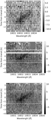 |
Fig. 7 Same as Fig. 6 but for He Iλ10833 lines. |
| In the text | |
|
Fig. 8 From left to right, the pre, ingress, start, center, end, and egress sections, as indicated by the colored areas. Hatched sections on night 2 refer to technical dropouts. Dashed and dotted lines show the four contact times. |
| In the text | |
|
Fig. 9 Hα transmission spectra for ingress, start, center, end, and egress phase from bottom to top (consecutively offset by 0.05; comoving planetary frame). Dashed lines show night 1 results, dotted lines night 2 results, and solid lines the average of these two. |
| In the text | |
|
Fig. 10 Transmission spectra in the He Iλ10833 line region for ingress, start, center, end, and egress phase from bottom to top (consecutively offset by 0.05; comoving planetary frame). Dashed lines show night 1 results, dotted lines night 2 results, and solid lines the average of these two. |
| In the text | |
|
Fig. 11 Superimposed transmission spectra in He Iλ10833 (solid) and Hα (dashed) for ingress, start, center, end, and egress phase from bottom to top (consecutively offset by 0.06). |
| In the text | |
|
Fig. 12 Synthetic (pseudo-)transmission signals caused by the CLV during individual temporal sections of the transit. |
| In the text | |
|
Fig. 13 Transmission light curves for Hα (top row, panels a–c) and He Iλ10833 (bottom row, panels d–f) for velocity bands (−50, −15) km s−1, (−15, +15) km s−1, and (+ 15, +50) km s−1 from left to right. Blue diamonds indicate night 1 and red circles indicate night 2. The solid yellow lines represent best-fit light curves from the circumplanetary annulus model, dash-dotted black lines are model light curves pertaining to the super-rotating wind model, and the green solid lines are those for the combined circumplanetary and up-orbit stream model. |
| In the text | |
|
Fig. 14 Sketch of the HAT-P-32 system (approximate scales). The planetary body (black circle) moves along its orbit (solid line). The direction of orbital motion is indicated by an arrow head. The planetary body is surrounded by an atmosphere (gray shade). The model up-orbit stream (black rectangle) originates from the first Lagrange point. |
| In the text | |
|
Fig. 15 Average transmission spectra along with best-fit models for annulus atmosphere (dashed), super-rotating wind (dotted), and up-orbit stream (solid) for the Hα line (left) and the He Iλ10833 lines (right). |
| In the text | |
|
Fig. 16 Solution to the hydrodynamic problem for the investigation of the Hα line. |
| In the text | |
|
Fig. 17 Synthetic transmission spectrum of HAT-P-32 b (red) in the Hα line for the conditions of Fig. 16. Wavelengths are shifted by systemic motion of HAT-P-32. |
| In the text | |
|
Fig. 18 Planetary He Iλ10833 absorption profile for the “center” phase (mid-transit, see Fig. 11) compared to two model absorption profiles for H/He ratiosof 90/10 (cyan) and 99/1 (red) (see Fig. 19) The vertical dotted lines indicate the positions of the lines. |
| In the text | |
|
Fig. 19 Outputs of the He hydrodynamics model showing the H and H+ densities (top), the radial wind velocity (middle), and the He (23S) density (bottom) obtained from the fit of the observed He (23S) absorption (see Fig. 18). Profiles are shown for the canonical H/He ratio of 90/10 (black) and for a high H/He ratio of 99/1 that resembles the model of Hα (red). The temperature was 14 000 K in both cases and the mass-loss rate of 3.6 × 10¹² g s−1 and 1.6 × 10¹³ g s−1, respectively. |
| In the text | |
|
Fig. B.1 Excerpt of the first spectrum on night 1 (blue dots) along with telluric absorption model (solid red) and locations of relevant water absorption lines (vertical dashed black). Hydroxide emission lines are indicated by shorter, dotted red lines. |
| In the text | |
|
Fig. B.2 The depth of the water column obtained with molecfit by fitting the NIR channel data as a function of time. |
| In the text | |
|
Fig. B.3 Mean sky spectrum during night 1 (black points) along with best-fit model (solid red line) and wavelengths of the Q1 and Q2 doublet lines according to Oliva et al. (2015) (f-components green dotted, e-components dashed blue vertical lines). Gray-shaded regions are exempted from the fit. |
| In the text | |
|
Fig. B.4 Ratio between strengths of the Gaussian model components representing the Q2 e (blue stars) and Q2f (red pluses) lines and the strength of the combined Q1 components along with best-fit relation (dashed black). |
| In the text | |
|
Fig. B.5 Equivalent width of the Q1 doublet as afunction of time. |
| In the text | |
|
Fig. B.6 Excerpt of normalized last spectrum from night 2 before (blue, dotted) and after (red, dashed) correction for OH emission lines. The correction for telluric absorption lines is also included. |
| In the text | |
|
Fig. C.1 Comparison of pre- and post-transit reference spectra. Top plot, top panel: Averaged, normalized pre-transit spectra (nos. 1,2,3) and post-transit spectra (nos. 20 − 23) around the He Iλ10833 lines during night 1. Dotted lines indicate the averaged spectra obtained without our telluric emission line correction. Top plot, bottom panel shows the ratio of the averaged post- and pre-transit spectra along with an estimate of the 95 % confidencerange resulting from noise (green shades). The bottom panels show the same for the Hα line region. |
| In the text | |
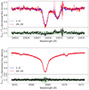 |
Fig. C.2 As Fig. C.1 but for night 2. |
| In the text | |
Current usage metrics show cumulative count of Article Views (full-text article views including HTML views, PDF and ePub downloads, according to the available data) and Abstracts Views on Vision4Press platform.
Data correspond to usage on the plateform after 2015. The current usage metrics is available 48-96 hours after online publication and is updated daily on week days.
Initial download of the metrics may take a while.