| Issue |
A&A
Volume 692, December 2024
|
|
|---|---|---|
| Article Number | A230 | |
| Number of page(s) | 14 | |
| Section | Planets, planetary systems, and small bodies | |
| DOI | https://doi.org/10.1051/0004-6361/202451003 | |
| Published online | 17 December 2024 | |
The overflowing atmosphere of WASP-121 b
High-resolution He I λ10833 transmission spectroscopy with VLT/CRIRES+
1
Thüringer Landessternwarte Tautenburg,
Sternwarte 5,
07778
Tautenburg,
Germany
2
Anton Pannekoek Institute for Astronomy, University of Amsterdam,
1090 GE
Amsterdam,
The Netherlands
3
Institut de Recherche en Astrophysique et Planétologie, Université de Toulouse, CNRS, IRAP/UMR 5277,
14 avenue Edouard Belin,
31400
Toulouse,
France
4
Universitäts-Sternwarte, Ludwig-Maximilians-Universität München,
Scheinerstraße 1,
81679
München,
Germany
5
Exzellenzcluster Origins,
Boltzmannstraße 2,
85748
Garching,
Germany
6
Institut für Astrophysik und Geophysik, Georg-August-Universität,
Friedrich Hund Platz 1,
37077
Göttingen,
Germany
7
Max-Planck-Institut für Sonnensystemforschung,
Justus-von-Liebig-Weg 3,
37077
Göttingen,
Germany
8
Department of Physics and Astronomy, Uppsala University,
Box 516,
75120
Uppsala,
Sweden
9
Instituto de Astrofísica de Andalucía – CSIC,
c/ Glorieta de la Astronomía s/n,
18008
Granada,
Spain
10
European Southern Observatory,
Karl-Schwarzschild-Str. 2,
85748
Garching bei München,
Germany
11
Hamburger Sternwarte, Universität Hamburg,
Gojenbergsweg 112,
21029
Hamburg,
Germany
12
Laboratory for Atmospheric and Space Physics, University of Colorado at Boulder,
600 UCB,
Boulder,
CO 80303,
USA
13
Department of Astronomy, University of Science and Technology of China,
Hefei
230026,
China
★ Corresponding author; This email address is being protected from spambots. You need JavaScript enabled to view it.
Received:
5
June
2024
Accepted:
14
November
2024
Abstract
Transmission spectroscopy is a prime method to study the atmospheres of extrasolar planets. We obtained a high-resolution spectral transit time series of the hot Jupiter WASP-121 b with CRIRES+ to study its atmosphere via transmission spectroscopy of the He I λ10833 triplet lines. Our analysis shows a prominent He I λ10833 absorption feature moving along with the planetary orbital motion, which shows an observed, transit-averaged equivalent width of approximately 30 mÅ, a slight redshift, and a depth of about 2%, which can only be explained by an atmosphere overflowing its Roche lobe. We carried out 3D hydrodynamic modeling to reproduce the observations, which favors asymmetric mass loss with a more pronounced leading tidal tail, possibly also explaining observational evidence for additional absorption stationary in the stellar rest frame. A trailing tail is not detectable. From our modeling, we derived estimates of ≥2 × 10¹³ g s−1 for the stellar and 5.4 × 10¹² g s−1 for the planetary mass loss rate, which is consistent with X-ray and extreme-ultraviolet (XUV) driven mass loss in WASP-121 b.
Key words: techniques: spectroscopic / planets and satellites: atmospheres / planets and satellites: individual: WASP-121 / X-rays: stars
© The Authors 2024
 Open Access article, published by EDP Sciences, under the terms of the Creative Commons Attribution License (https://creativecommons.org/licenses/by/4.0), which permits unrestricted use, distribution, and reproduction in any medium, provided the original work is properly cited.
This article is published in open access under the Subscribe to Open model. This email address is being protected from spambots. You need JavaScript enabled to view it. to support open access publication.
1 Introduction
The ultra-hot Jupiter WASP-121 b revolves around an F6V type star (Delrez et al. 2016). Its orbit is highly misaligned, nearly polar, and puts the planet only about 15% above the Roche limit, close to the regime of tidal disruption (Delrez et al. 2016; Seidel et al. 2023). The planet WASP-121 b fills 59% of its Roche lobe volume and is aspherical owing to tidal forces (Delrez et al. 2016). In Table 1, we list the relevant system parameters.
WASP-121 b has become a coveted target for follow-up observations of all kinds. Specifically, the spectral signatures of numerous atomic and molecular species were detected in the atmosphere of WASP-121 b (Sing et al. 2019; Hoeijmakers et al. 2020; Borsa et al. 2021; Merritt et al. 2021; Gibson et al. 2022; Azevedo Silva et al. 2022; Maguire et al. 2023; Ouyang et al. 2023). Time variability of the atmospheric signal, potentially attributable to planetary weather patterns (Changeat et al. 2024), has been suggested in several studies (e.g., Wilson et al. 2021; Ouyang et al. 2023), whereas other studies report no evidence for such variation (e.g., Maguire et al. 2023).
The atmosphere of WASP-121 b is thought to undergo Roche lobe overflow driven by optical and infrared light (Huang et al. 2023). Salz et al. (2019) find evidence for an extended atmosphere by means of excess in-transit ultraviolet absorption, and Maguire et al. (2023) report blue-shifted planetary absorption features of neutral hydrogen, Fe II, and Ca II with strengths inconsistent with the material being confined to within the Roche lobe. Likewise, WASP-121 b shows Na I D absorption with a variable blueshift, which increases from −3.8 km s−1 during the first half to −6.6 km s−1 during the second half of the transit and shows a resolution-corrected full width at half maximum (FWHM) of about 13 km s−1 (Seidel et al. 2023). Atmospheric modeling constrained by the observed Hα line absorption feature yields an estimate of 1.3 × 10¹² g s−1 for the planetary mass loss rate (Yan et al. 2021).
The infrared phase curve observed with the Spitzer telescope leads to brightness temperature estimates of about 2700 K and 700–1100 K on the planetary day- and nightside, respectively (Morello et al. 2023). While the analysis by Morello et al. (2023) indicates a westward offset of the hotspot with respect to the substellar point, the study by Mikal-Evans et al. (2023), who used observations with NIRSpec onboard the James Webb Space Telescope, favors an eastward shift. Further evidence of the dynamic state of WASP-121 b’s atmosphere is reported by Mikal-Evans et al. (2022), whose results indicate day-side warming and night-side cooling in its stratosphere. The analysis of Hubble Space Telescope (HST) observations by Changeat et al. (2024) is consistent with a day-side temperature inversion, starting at a pressure level of 0.1 bar, and Hoeijmakers et al. (2024) find evidence for night-side condensation of titanium. Although many studies of WASP-121 b’s atmosphere exist, no high-resolution observations of the important He I λ10833 line have been published as of yet, which is precisely the point of the paper at hand.
Relevant system parameters of WASP-121.
2 Observations and data reduction
2.1 High-resolution spectroscopy with CRIRES+
During the night from 21 to 22 Feb. 2023, we used CRIRES+ (Dorn et al. 2023) mounted at the Very Large Telescope (VLT) to observe a spectral transit time series of WASP-121, which consists of 40 consecutive exposures with an individual integration time of 450 s. The observations were taken in the Y-band with the Y1029 wavelength setting. Using the 0.2″ slit, we obtained a nominal spectral resolution of about 100 000. We adopted an ABBA nodding pattern, which places the target in a sequence of distinct A and B positions on the slit. This allowed us to efficiently remove the sky background as well as to remedy instrumental effects. In Fig. 1, we show the mean S/N in the vicinity of the He I λ10833 lines along with the evolution of the airmass.
The data were reduced using the CRIRES+ pipeline cr2res available from ESO1. In a first step, the associated raw calibration frames, taken as part of the observatory’s daily calibration routine, were processed using the standard calibration cascade as described in the CRIRES+ Pipeline User Manual. This step produces the so-called processed calibrations, that is, the bad pixel mask, the normalized flat field, and the trace-wave file containing the wavelength solution and detector location for each spectral order. In a second step, the raw science frames were reduced using the cr2res_obs_nodding recipe, which applies the processed calibrations to the science frames, subtracts the B from the A frames in each AB (or BA) nodding sequence, and uses optimal extraction to produce one-dimensional science spectra, to which, finally, the wavelength solution is applied.
We carried out a telluric correction with molecfit (Smette et al. 2015; Kausch et al. 2015). The models were also used to refine the wavelength solution. In Fig. A.1, we show the shift of the best-fit wavelength solution obtained by molecfit with respect to that of the pipeline. Overall, a slight blueshift of about 0.1 km s−1 and a nodding-dependent pattern with about the same semi-amplitude is observed. From the molecfit solution, we estimated a value of 101 900 ± 660 for the instrumental spectral resolution (Fig. A.2); the value and methodology are similar to that reported by Yan et al. (2023). While the small formal statistical uncertainty of the spectral resolution may be too optimistic given possible variation across the detector, no evidence for any change in time was found during our observing run. Taking into account the phase smearing caused by the finite exposure time of 451 s per integration, we estimated an effective spectral resolution of 61 600 for a planetary signal moving along on the orbit (see Czesla et al. 2022; Boldt-Christmas et al. 2024).
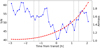 |
Fig. 1 Mean S/N per spectral bin (blue squares) in the 10 830–10 840 Å range and the airmass (red circles) for the spectral time series. Vertical dotted lines indicate the optical first to fourth contact. |
2.2 High-energy stellar spectrum
The population of the metastable helium level, giving rise to the He I λ10833 triplet transitions, is intimately related to the high-energy extreme ultraviolet and X-ray radiation field, which makes the latter a crucial ingredient in the interpretation of any He I λ10833 transmission signal (e.g., Sect. 3.5).
The stellar spectral energy distribution (SED, Figure 2) used in our analysis has been observed and constructed as part ofHST program 16701. The SED was constructed in a similar routine to those of the MUSCLES program Loyd et al. (2016), with some differences which we describe here.
The ultraviolet and optical regions combine G140L data from Program 16701 with archival E230M, G430L and G750L observations obtained as part of the Panchromatic Comparative Exoplanetology (PanCET) program (Evans et al. 2018). The G140L data was obtained on 2022 December 06 over 3 HST orbits with the G140L grating with a total exposure time of 6680 s. For the G140L and E230M observations we combined all available spectra with an error-weighted coadd. The orders of the E230M spectra were combined by coadding each overlap region. Multiple emission lines are detected in the G140M spectrum, along with stellar continuum flux at wavelengths ≳1400 Å.
Unfortunately, no flux is detected at Lyman α due to ISM absorption. We therefore used the reconstructed Lyman α line of Procyon from Cruz Aguirre et al. (2023), which has similar stellar parameters to WASP-121. The line profile was scaled to the squared radius and distance ratios of the two stars.
For the optical data we selected the spectra with the longer exposure times from Evans et al. (2018) and combined them, coadding 12 G430L datasets and 5 G750L datasets. We did not exclude the in-transit spectra as the overall flux difference is only ~ 1 %. The red end of the G750L spectra were strongly affected by fringing, which was removed using the STISTOOLS.DEFRINGE routine.
For the X-ray region WASP-121 was observed with XMM-Newton for 9 ks (Obs. ID 0804790601, PI Sanz-Forcada) and fit with an Astrophysical Plasma Emission Code (APEC) model (Smith et al. 2001); a preliminary analysis of the data is also presented in Evans et al. (2018). With the FUV and X-ray combined, we filled in the currently unobservable extreme-ultraviolet (EUV) range (≈ 100–1000 Å) using a method based on the differential emission measure (DEM, Duvvuri et al. 2021). Longer Wavelengths not covered by STIS spectra (1720-2280 Å, > 10230 Å) use a PHOENIX BT-Settl (CIFIST) model (Allard 2016) retrieved from the SVO Theoretical spectra web server2 converted into vacuum wavelengths. Stellar parameters used to produce and scale the model (Teff,★, log(𝑔), radius, and distance) were taken from Delrez et al. (2016).
By integrating the reconstructed SED, we found the stellar luminosities and corresponding fluxes at the planetary distance listed in Table 2. Adopting the bolometric brightness of (3.3 ± 0.3) L⊙ (Delrez et al. 2016) and the flux at wavelengths shorter than 100 Å for the X-ray luminosity, we found a  value of −4.99 ± 0.04 for WASP-121. The X-ray luminosity of WASP-121 is consistent with emission at the empirical X-ray saturation limit for F-type stars (Pizzocaro et al. 2019), which is expected given the short stellar rotation period of <1.13 d (Bourrier et al. 2020).
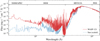 |
Fig. 2 Spectra energy distribution of WASP-121, with the sources of each wavelength region labeled at the top. The SED is compared with that of the Sun scaled to the same bolometric luminosity. |
Stellar luminosities of WASP-121 and fluxes at the planetary orbital separation of WASP-121 b for various spectral bands.
3 Results
3.1 Roche geometry
As WASP-121 b orbits at close orbital distance, the shape of the planet and its Roche lobe deviate considerably from the spherical approximation (Delrez et al. 2016). The planetary radius, Rp, listed in Table 1 was derived from photometry obtained by the Transiting Exoplanet Survey Satellite (TESS) and corresponds to the effective radius of a spherical planetary disk. Adopting a Roche model (available through PyAstronomy, Czesla et al. 2019), we computed the planetary geometry. For the radii of the first and second Lagrange points, situated along the axis connecting the star and the planet, we found values of 3.43 RJup and 3.59 RJup, respectively. Further, we estimated a value of 1.77 RJup for the planetary radius as seen within the orbital plane (Rside) and 1.735 RJup perpendicularly out of the plane (Rpole), which define the appearance of the planet during conjunction. These values are consistent with those given by Delrez et al. (2016)3. We further found 2.31 RJup for the extent of the Roche lobe along the side and 2.21 RJup for its height above the orbital plane. The entirety of the Roche lobe covers 2.5% of the stellar disk during conjunction, but only 1 % is left for the approximately annulus-shaped region not blocked by the opaque planetary body, which is available for transmission by a gravitationally bound atmosphere. Therefore, any transmission signal deeper than that during conjunction cannot be caused by material confined to within the Roche lobe.
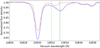 |
Fig. 3 Out-of-transit master spectrum of WASP-121 around the He I λ10833 triplet lines in the stellar rest frame (blue) along with synthetic model (red). The wavelengths of the He I λ10833 triplet lines are indicated by dotted green lines. |
3.2 Systemic radial velocity
Delrez et al. (2016) report a value of 38.350 ± 0.021 km s−1 for the systemic velocity of WASP-121 (Table 1). This value is consistent with the less precise measurement of 38.36 ± 0.43 km s−1 by Gaia (Gaia Collaboration 2023). As a cross-check, we determined the systemic radial velocity from our own data. Specifically, we fit the spectral region between 10780 Å and 10 828 Å using a synthetic PHOENIX spectrum (Teff = 6500 K, log 𝑔 = 4.50, solar metallicity, Husser et al. 2013). In the fit, we assumed the projected rotational speed of 13.56 km s−1 determined by Delrez et al. (2016) and included a free normalization by a first-order polynomial, the coefficients of which we treat as nuisance parameters. The resulting estimate is 38.4 ± 0.3 km s−1, which is consistent with the more precise value by Delrez et al. (2016), which we adopt in our analysis.
3.3 The stellar He I λ 10833 lines
The He I λ10833 triplet lines are regularly observed primarily in active stars (e.g., Sanz-Forcada & Dupree 2008; Fuhrmeister et al. 2019). In Fig. 3, we show the out-of-transit master spectrum of WASP-121 along with the PHOENIX model used in Sect. 3.2 for reference. Although the model does not perfectly reproduce the observation, in particular, the strong silicon line at about 10832 Å, the comparison clearly indicates excess absorption at the wavelengths of the He I λ 10833 triplet lines, which are not included in the PHOENIX model.
Using a model consisting of four Gaussian component to represent the silicon as well as all of the three He I λ10833 triplet lines, we estimated an EW of 115 ± 5 mÅ for the blended two stronger components of the He I λ10833 triplet lines. Yet, the blend is additionally contaminated by photospheric lines at a wavelength of about 10 832.5 Å, which include an Fe II line. These lines are reproduced by the PHOENIX model. Subtracting the latter prior to the fit, we obtained a contamination-corrected estimate of 96 ± 5 mÅ. In combination with a  value of about −5 (Sect. 2.2), the result is entirely consistent with the properties of the dwarf sample presented by Sanz-Forcada & Dupree (2008).
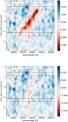 |
Fig. 4 Maps of transmission spectra and residuals (smoothed) of the He I λ10833 region in the stellar reference frame. The top panel shows the observed transmission spectra and the bottom panel the residuals after subtraction of the best-fit model (color coded). The horizontal lines (black dashed) indicate the optical first to fourth contact times, dotted yellow lines (vertical) show the location of the telluric OH line components, the dash-dotted magenta line indicates the wavelength of the stellar He I λ10833 line, and the dashed red line (diagonal) shows the radial velocity track of the planetary orbit. |
3.4 Transmission spectroscopy
To construct an out-of-transit reference spectrum, fref, we first shifted all spectra into the stellar reference frame and obtained an error-weighted average of the spectra with the running numbers 1–10 and 36–40 (Appendix A). We then generated transmission spectra, by dividing the individual spectra by the reference. In Fig. 4, we show the thus obtained map of transmission spectra, T (λ, t), as a function of wavelength, λ, and time, t. The map shows a pronounced absorption signal mostly following the radial velocity track of the planetary orbit. Moreover, the map indicates that potential additional absorption components, apparently stationary in the stellar rest frame during the first half of the transit, may exist. To study the signals more quantitatively, we proceeded to construct empirical and physical models of the transmission spectrum.
3.4.1 Empirical modeling of the time-dependent transmission spectrum
We modeled the time-dependent transmission spectrum, T (λ, t), shown in Fig. 4 using an empirical model similar to the one applied by Salz et al. (2018) and Czesla et al. (2022). In particular, we approximate the planetary atmosphere as a slab of constant column density, and use the ansatz
 (1)
(1)
to model the transmission spectrum, where fa(t) denotes the time-dependent disk filling factor of the model atmosphere, which is the fraction of the stellar disk covered by it, and τ(λ, t) is the optical depth, given by
 (2)
(2)
Here, nC is the number of assumed He I λ10833 absorbing components within the slab with distinct column densities of helium in the metastable 3S1 state, NHe I,n, velocity shifts, vn(t), and intrinsic widths, σin,n, which summarizes all remaining broadening, e.g., caused by thermal motion or velocity dispersion. The absorption cross section is given by σHe I. The index j enumerates the three lines forming the He I λ10833 triplet, G represents a Gaussian profile centered on the Doppler-shifted wavelength of the respective triplet line, λHe I,j. Its width is determined by the quadratic sum of the intrinsic width, σin,n, and a systematic term, σsys, representing the effects of phase smearing and the instrumental resolution. Although instrumental broadening and phase smearing affect the spectrum rather than the optical depth, this approximation is usually viable (see Czesla et al. 2022, Appendix G).
In our modeling, we found a single absorption component (nC = 1) to be sufficient to explain the bulk of the observed signal (Fig. 4). This component is set up such that it moves along with the planetary orbital velocity, vorb, but may show a velocity offset, ∆v, so that
 (3)
(3)
Here and in the following, we drop the index n = 1 for improved readability. The remaining free parameters of the model are the column density of the atmosphere, NHe I and the intrinsic width of the absorption profile, σin, which are both considered as independent of time. As the filling factor and the column density are strongly correlated, they cannot be determined independently here. Therefore, we implement only a time-dependent filling factor, fa(t), by adopting one free parameter, fa,k with 1 ≤ k ≤ 40, for the time-averaged filling factor valid for the time intervals covered by each of our 40 spectra. Altogether, we are left with a total of 43 free parameters. The use of a single absorption component is certainly a strong simplification of the true atmospheric structure (Sect. 3.5), but is nonetheless justifiable if the bulk of absorption occurs in an outer, optically thin region producing weak line saturation (e.g., Wang & Dai 2021) and the overall velocity structure results in an approximately Gaussian line profile.
In models based on Eqs. (1) and (2), the disk filling factor and the optical depth, or equivalently, the column density of absorbers, are highly degenerated in the optically thin regime defined by the validity of the approximation exp(−τ(λ, t)) ≈ 1 − τ(λ, t). If assumed to hold, only the product of the filling factor and the absorber column density can be determined. This also means that no reliable estimate for the upper limit of the atmospheric extent can be obtained from such a model; some constraints may be derived though from the transit duration (see Sect. 3.4.2). To mediate the impact of this degeneracy on the model fitting, we implemented the model using a reference filling factor, fR, and defined shape parameters, 0 ≤ fs,k ≤ 1, which define the shape of the transmission light curve, such that
 (4)
(4)
To find the optimal parameters for the model, we carried out a maximum likelihood fit to the data shown in the top panel of Fig. 4 using Powell’s method (Powell 1964). During the fit, we fixed the reference filling factor, fR, to a value of 10% to avoid the aforementioned strong correlation with the column density. Meaningful values for the velocity shift, the broadening, and the shape parameters can be derived in this fashion. The maximum likelihood parameters are listed in Table 3 and a map of the remaining residuals after subtraction of the best-fit model is shown in the bottom panel of Fig. 4.
We then used the emcee package (Foreman-Mackey et al. 2013) to derive uncertainties by Markov-Chain Monte-Carlo (MCMC) sampling from the posterior, adopting uniform priors for all values within their natural limits. To mitigate the impact of parameter degeneracy, the sampling was done in a two-step approach. Firstly, we fixed all shape parameters to their best-fit values and sampled from the posteriors for the broadening parameter, velocity shift, reference filling factor, and column density. In Table 3, we give the 68% highest probability density (HPD) credibility intervals along with the maximum likelihood estimates. As the reference filling factor and column density are strongly correlated in the model, we only consider their product. Filling factors smaller than 2.5% are disfavored by the model, but this result strongly hinges on the adopted slab geometry. Secondly, we fixed all variables but the shape parameters to their best-fit values and sampled from their posteriors. Through an analysis of the autocorrelation function of the individual chains, we ensured that for each parameter 100 or more independent samples were obtained (e.g., Sharma 2017).
3.4.2 Transmission light curves in the planetary frame
In the top panel of Fig. 5, we show the temporal evolution of the shape parameters (Table 3), which represent the strength of He I λ10833 absorption. The bottom panel of the same figure shows the light curve extracted from a narrow, ±0.25 Å wide band, centered in the wavelength of the stronger doublet of the He I λ10833 triplet in the planetary reference frame. This region is the most sensitive to absorption in the planetary frame. The shape of these curves is reminiscent of typical optical transit light curves.
In principle, the duration of the transit event constrains the extent of the atmosphere along the direction of planet motion. To study this aspect, we approximated the atmosphere by an annulus with inner radius, Rin, taken to be identical to the effective planetary radius, Rp (Table 1). For the sake of the transit modeling, the inner part of the annulus was treated as transparent and the outer radius, Rout, was considered as a free parameter. To model the transit of the annulus-shaped atmosphere, we adopted the light curve solutions published by Mandel & Agol (2002) and used a linear limb darkening coefficient of 0.4, suitable for F-type stars in the Y-band (e.g., Claret et al. 1995). As the models by Mandel & Agol (2002) are valid for a completely opaque body, we introduced an additional scaling factor to fit the data.
In Fig. 5, we show model light curve for an assumed outer radius of 2.7, 4, and 8 Jovian radii with the scaling factor adapted to best match the data. In the case of the transmission light curve in the lower panel, the scale factor represents the atmospheric transparency. Evidently, the transit duration of the atmosphere must be longer than that of the opaque planetary body, however, the effect is not particularly pronounced compared to the temporal sampling of our spectral time series. While the narrowband He I λ10833 light curve provides some evidence for an early ingress of the signal of potentially physical origin (Sect. 3.5), this effect is less pronounced when looking at the evolution of the values of the shape parameters. We found no evidence for significant post-transit absorption in our data. Altogether, this favors an atmosphere with the bulk of He I λ10833 absorption remaining constrained to within a region close to the planet, although the weak relation between extent (i.e., outer radius in our model) and transit duration does not allow us to strongly constrain this volume.
Best-fit parameters and uncertainties for our empirical modeling.
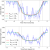 |
Fig. 5 Time evolution of He I λ10833 transmission. The temporal evolution of the shape parameters (top panel) and the narrow-band, ±0.25 Å He I λ10833 transmission light curve in the bottom panel. Solid lines indicate transit models for an annulus-shaped atmosphere with various outer radii and the vertical dotted lines mark the optical contact point. |
3.4.3 Light curves in the stellar frame
The discovery of giant tidal tails in the exoplanet HAT-P-32 b (Czesla et al. 2022; Zhang et al. 2023) is largely based on variability of the He I λ10833 line in the stellar frame. While the bottom panel of Fig. 4 does not show pronounced residuals at the wavelength of the He I λ10833 line in the stellar rest frame, some residuals are present particularly in the first half of the transit. Because the pre- and post-transit spectra were used to construct the reference spectrum by which the individual spectra were divided, an absorption component in the stellar frame invariant on the timescale of the observation would not show up in the residuals. Yet, a change in the absorption of such a He I λ10833 line would still be visible. In Fig. 6, we show a light curve extracted from a ±0.5 Å region (±14 km s−1) around the wavelength of the He I λ10833 line before and after the subtraction of our best-fit empirical model, corresponding to the data in the upper and lower panel of Fig. 4.
Prior to the subtraction of the model, the light curve prominently shows the transit of He I λ10833 absorbing material being dragged along with the planet. This signal is strongly reduced by the model subtraction. The light curve after subtraction still shows a relatively short (≈20 min) dip about centered on the first optical contact point, as suggested by Fig. 6, and a potential slight overall increase toward the end of the time series. The variability in the light curve reflects changes in the center of the He I λ10833 line profile during the observation, which may be caused by stellar activity, a change in the atmospheric absorbing column, or unphysical effects such as the data reduction.
To assess the impact of the Rossiter-McLaughlin effect and the center-to-limb variation on the result (Yan et al. 2015; Czesla et al. 2015), we used a simulation. In particular, we constructed a synthetic spectral transit time series based on limb-angle resolved stellar spectra and a discretized, rotating stellar surface eclipsed by the opaque planetary disk (for details see Czesla et al. 2022). This setup accounts for both the effects of the Rossiter-McLaughlin effect and the center-to-limb variation. As the He I λ10833 triplet lines are produced in the chromosphere, they are not reproduced by synthetic photospheric spectra. To incorporate the effect of the stellar He I λ10833 lines nonetheless, we included an ad-hoc He I λ10833 line, whose disk-averaged properties match those observed in WASP-121 (Sect. 3.3). The details of the center-to-limb variation of the He I λ10833 triplet lines in WASP-121 remain unknown. Therefore, we used the quiet Sun as an inspiration, in which the triplet becomes weaker toward the limb. To estimate the maximum interference, we assumed extreme limb darkening for the triplet lines, so that they vanish at the limb. For the specific case of the light curve shown in Fig. 6, the variation caused by these effects remains below about 8 × 10⁻⁴, which is negligible compared to other factors of variation.
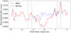 |
Fig. 6 Light curve extracted from a ±0.5 Å region around the rest wavelength of the He I λ10833 line before (solid red) and after (dashed blue) subtraction of the best-fit empirical model. |
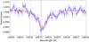 |
Fig. 7 Averaged transmission spectrum between optical second and third contact. The red lines show three best-fit empirical models with 5% filling factor and one (dashed) and two (solid) absorbing components. The vertical dotted lines show the wavelengths of the He I λ10833 triplet lines. |
3.4.4 Time-averaged transmission spectrum
In Fig. 7, we show the time-averaged transmission spectrum obtained between the optical second and third contacts (spectra with nos. 16–32). The transmission spectrum shows a prominent signal at about the wavelength of the He I λ10833 line and a potential secondary signal, which shows significant redshift in the planetary rest frame. This latter component is related to the residual structure, approximately stationary in the stellar rest frame, shown in the bottom panel of Fig. 4. Using the synthetic spectra introduced in Sect. 3.4.3, we estimated that the spectral effects introduced into the transmission spectrum by the center-to-limb variation and the Rossiter-McLaughlin effect remain below 10−3 in the vicinity of the He I λ10833 line. While this effect is, therefore, not a plausible explanation for the secondary absorption component, stellar activity can affect the stellar He I λ10833 line cores.
We approximated the transmission spectrum using the same model as used in Sect. 3.4.1. Here, we specifically adopted a filling factor of 5% for the atmosphere, which is large enough to put it into the optically thin regime and remains fixed in our modeling. We assumed either one or two absorption components to approximate the data and show the best-fit models in Fig. 7. In the model with one component, the absorption is approximately centered on the wavelength of the He I λ10833 triplet. The optional second component is redshifted by about 40 km s−1 . Adding the second component improved the Bayesian Information Criterion (BIC, e.g., Jeffreys 1932; Kass & Raftery 1995) of the fit by 46, which constitutes strong formal evidence in favor of additional absorption in the red flank of the line. A possible physical explanation for its presence is provided by our three-dimensional modeling.
3.5 Three-dimensional modeling of the outflow
As demonstrated in Sect. 3.4, the planetary atmosphere overfills the Roche lobe, so that the escaping gas is possibly dragged into an orbital shear, which can lead to the formation of tail-like outflows leading and trailing the planet. To simulate the planetary outflow and its interaction with the host star’s stellar wind and gravitational field, we used three-dimensional (3D) hydrodynamic models. Our focus is on the dynamics of the outflow rather than thermodynamics. The simulation did neither incorporate chemical effects nor the heating and cooling rates. We performed a radiative transfer analysis during the post-processing to determine the ionization fractions and excitation of helium and hydrogen. This allowed us to investigate how the escaping planetary gas impacts the He I λ10833 transmission spectra.
Specifically, we used the 3D Eulerian (magneto) hydrodynamic code Athena++4 (version 2021, Stone et al. 2020). Building upon the methodologies described in Sect. 2 of MacLeod & Oklopčić (2022), we adopted their simulation setup and radiative transfer code, which has been further developed to account for planetary day-night anisotropies as detailed in Nail et al. (2024b). In the following, we highlight the core features of our simulations and discuss the specific modifications introduced for this study.
The computational domain ranged from r = R*, to r = 1.01433 × 1014 cm (6.78 au), covering the full solid angle of 4π steradians. The primary mesh was divided into 18 × 12 × 16 mesh blocks, each with 16 zones. For the region around the planet, we adopted three nested levels of static mesh refinement. We employed an ideal gas equation of state, P = (γ − 1)ϵ, with γ = 1.0001 denoting the gas adiabatic index. This choice ensures that the gas remains nearly isothermal along adiabatic processes. However, the specific entropy of the wind differs between the star and the planet and the temperature along the planet’s surface can be adjusted as described in Nail et al. (2024b). Based on the distribution of gas in a snapshot obtained after 4 orbits, when convergence was reached, we derived transmission spectra of the He I λ10833 lines by applying a radiative transfer analysis. We adopted a solar-like gas composition characterized by mass fractions of hydrogen (X = 0.738), helium (Y = 0.248), and metals (Z = 0.014) uniformly throughout the computational domain. Assuming steady state, each simulation grid cell was in a state of detailed equilibrium. The unattenuated photoionization rate (Φ) was determined using the irradiating stellar flux of WASP-121 (Sect. 2.2). Higher optical depths in our simulations necessitate more iterations to determine ion populations than in MacLeod & Oklopčić (2022) (see their equations 9 and 10). The updated radiative transfer code, as well as the simulation snapshot, can be found on Zenodo5.
To constrain the physical conditions leading to the observed transmission spectrum of WASP-121b, various parameter configurations were tested. To reproduce the observations, we found that a relatively high value for the hydrodynamic escape parameter
 (5)
(5)
on the planetary day side was needed. A high value for the escape parameter leads to a cooler, tidally confined planetary wind. Combined with a day-side dominated outflow, this produces a stronger leading tail, better matching the additional absorption in the red flank of the observed planetary He I λ10833 line. In contrast, a low escape parameter results in a hotter, more radial, bubble-shaped outflow, where only a trailing tail forms (see Nail et al. 2024a). Specifically, we adopted a value of eight, which corresponds to an outflow temperature of ≈10 600 K and a sound speed, cs, of ≈12 km s−1. Varying λp by ±1 only marginally affected the resulting model transmission spectrum.
Our findings indicate that the morphology of the planetary wind is influenced by the balance between wind energy and gravitational forces. When the wind energy significantly exceeds the energy required to overcome the planet’s gravitational pull, the atmosphere escapes uniformly, forming a spherical or bubblelike shape. Conversely, when gravitational forces dominate, indicated by a high value of λp, the escaping gas is channeled through the Lagrangian points, resulting in long, thin streams. Figure 8 illustrates the density distribution of metastable helium and the line-of-sight velocity distribution of the gas in the orbital mid-plane for our best-matching simulation during mid-transit. Our findings indicate that the outflow is anisotropic. In particular, the outflow from the day side is stronger, which produces a pronounced leading tail with gas moving away from the observer. As the optical depth contours in Fig. 8 reveal, a significant portion of the line forms in the red-shifted leading tail. We propose that such a structure can account for the observed red-shifted secondary feature in the averaged transmission spectrum shown in Fig. 9, but note that the simulations suggest a spectral component smoothly varying in time as demonstrated by the time series maps shown in Fig. B.2.
The day-night anisotropy should not be excessively strong, as this would result in a larger than observed blueshift. In our best-matching simulation, we used a pressure ratio of 40% between the sub- and anti-stellar points, corresponding to a night-side outflow temperature of about 4200 K assuming a mean molecular weight of µ = 0.6 for an ionized atmosphere.
In our hydrodynamic simulations, it is possible to vary density and pressure simultaneously within a single snapshot without changing the flow dynamics, as long as the ratio between the pressure and density values is preserved. Using this approach, we adjusted the density and pressure of the simulation snapshot to ensure that the resulting transmission spectra match the observed absorption depth. We present two specific cases, dubbed density I and II. The former represents our best-matching model and the latter represents a setup with the density and pressure elevated by a factor of 2.0. In Fig. 9, we show the resulting model transmission spectra along with the binned observational spectrum.
To facilitate comparison with the observational data, we averaged the model spectrum between the second and third contact points of the transit. The shaded regions show the range of the modeled transmission spectra, indicating the variability of the model transmission signal during transit. We estimated a planetary mass loss rate of ṁp = (5.41 ± 1.10) × 1012g s−1, which is about an order of magnitude lower than the value of 7.3 × 10¹³ g s−1 derived by Huang et al. (2023) (their case D) primarily through the modeling of various metal lines, and about a factor of four higher than the result of 1.3 × 10¹² g s−1 derived by Yan et al. (2021) in their modeling.
The blue solid line in Fig. 9 represents the outcome of the density II setup; the corresponding optical depth contours are indicated by dotted lines in Fig. 8. The increased density causes the line-forming region to move away from the planet. Although the density II model cannot reproduce the depth of helium absorption, we hypothesize that a plausible explanation for the secondary redshifted feature in the observed spectrum lies in a large leading stream. This higher-density region, moving ahead of the planet, is also evident in the vertical structure of the outflow (see Fig. B.1 at phase −0.03). The line of sight velocity at that phase is approximately 50 km s−1, which is in alignment with the observed velocity shift of the secondary redshifted feature.
In Fig. B.2, we present a time series of He I λ 10833 transmission spectra. While the synthetic spectral line traces the planetary motion, and the core absorption does not significantly extend into the pre- or post-transit phases, the secondary component’s absorption may extend into the pre-transit phase and, although it also follows the planetary movement, it is sufficiently redshifted to appear approximately at the wavelength of the He I λ 10833 lines in the stellar rest frame. If the trailing arm were equally dense, as expected from an isotropic planetary outflow, a similar blue-shifted feature would emerge. However, this scenario does not align with our observations, thereby strengthening the hypothesis of a day-side dominated outflow. We found that the stellar mass loss rate needs to be high enough to clear the orbit of gas that would produce extended pre- and post-transit absorption. Based on the simulation, we found a stellar mass loss rate of ≈2 × 10¹³ g s−1 to be sufficient for that (see Table 4).
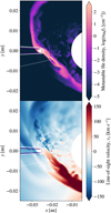 |
Fig. 8 Simulated metastable helium number density (top) and the line-oſ-sight velocity (bottom) in the orbital mid-plane of the WASP-121 system. The host star, located at the coordinate origin, is orbited by the planet, located on the negative x-axis, in counterclockwise direction. The observer is also located on the negative x-axis. The bottom panel shows the velocity component in the x-direction, representing the observer’s view during mid-transit. Purple and white contours indicate the cumulative optical depth at the center of the He I λ10833 line, with τ = 10 and τ = 1, respectively; solid and dotted contours represent the density I and II setup. The planetary outflow forms a red-shifted, leading tail, which originates from the more pronounced day side outflow. |
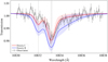 |
Fig. 9 Synthetic transmission spectra derived from our 3D simulation for the density I (red solid line) and density II (blue solid line) setups. As for the underlying observations (gray), a time average between the optical second and third transit contact is displayed. The shaded regions represent the range of model transmission spectra obtained during the transit. The synthetic spectra are multiplied by a factor of 1.00191 (Sect. 3.4.4) to match the observational continuum. The red solid line aligns well with the observed helium triplet, while the location of the secondary red component can be reproduced by considering a higher density of the same outflow structure. |
Line characteristics as well as the planetary and stellar mass loss rates obtained from the three-dimensional modeling.
4 Discussion
4.1 Planetary mass loss driven by XUV radiation
The strong XUV irradiation experienced by WASP-121 b (Table 2) is thought to lead to hydrodynamic mass loss. Our 3D modeling in Sect. 3.5 and the He I λ 10833 transmission spectrum constrain the planetary mass loss rate to about 3 × 10¹² g s−1. Assuming energy-limited escape (e.g., Watson et al. 1981; Lammer et al. 2003), an alternative estimate of the planetary mass loss rate, Ṁp,EL, can be obtained without consulting our transmission spectrum by application of the relation
 (6)
(6)
(see, e.g., Sanz-Forcada et al. 2011; Salz et al. 2016). Here, G is the gravitational constant, K allows us to include Roche lobe effects (Erkaev et al. 2007), the factor β ≥ 1 permits us to take into account XUV absorption radii larger than the optical planetary radius, and η is the heating efficiency. For the latter, Salz et al. (2016) recommend a value of approximately 0.1 for WASP-121 b, which has a gravitational surface potential of 1.2 × 10¹³ erg g−1 neglecting tidal effects. A value of ≲ 0.1 is also favored by the analysis of Lampón et al. (2023), which tends to put WASP-121 b into the recombination-limited flow regime, characterized by strong radiative cooling losses (Murray-Clay et al. 2009), generally expectable for highly irradiated planets according to Lampón et al. (2023). Following Erkaev et al. (2007) in adopting the average of the radii of the first and second Lagrange points as an effective Roche lobe radius, we found a value of 0.31 for K. Further substituting one for β and 330 900 erg cm−2 s−1 for fXUV (Table 2), we obtained an estimate of 4.4 × 10¹² g s−1 for the energy-limited planetary mass loss rate. This value is evidently consistent with the one resulting from our more comprehensive analysis.
Comparison of systems with detected or expected extended atmospheres.
4.2 Planetary atmospheres with large tails
Our observational results as well as our empirical and physical 3D modeling show that the bulk of He I λ10833 absorption in WASP-121 b occurs in an atmospheric structure within a few planetary radii around the planetary body. In addition, we found hints for He I λ10833 absorption by a leading tail with no observationally detectable trace of a trailing tail. So far, He I λ10833 transmission spectroscopy has revealed outflow morphologies with leading and trailing tails in the planets HAT-P-32 b (Czesla et al. 2022; Zhang et al. 2023) and HAT-P-67b (Gully-Santiago et al. 2024). In both of these systems, the leading tail has been found to be more pronounced, which is thought to be a consequence of asymmetric mass loss caused by the stronger heating of the planetary day side. Insofar, our findings in WASP-121 b are consistent. Yet, in the HAT-P-67 and HAT-P-32 systems, the outflowing streams are detectable in He I λ10833 across longer orbital phase ranges than for the WASP-121 system. In contrast, WASP-69 b, WASP-107 b, and HAT-P-18 b show a pronounced trailing tails without a detection of a leading counterpart (Nortmann et al. 2018; Spake et al. 2021; Fu et al. 2022; Tyler et al. 2024).
In Table 5, we list the mean densities, the ratio between sub-stellar and polar planetary radius (X), and the X-ray fluxes at the planetary separation for the aforementioned systems as well as WASP-12 b, in which the existence of a large atmospheric structure potentially similar to the ones observed in HAT-P-67 b and HAT-P-32 b has been suggested by observational and theoretical efforts (e.g., Li et al. 2010; Haswell et al. 2012; Fossati et al. 2013; Jensen et al. 2018; Wang & Dai 2021). The observational picture here remains, however, puzzling as recent high-resolution transit time series failed to produce evidence for He I λ10833 or, in fact, any other studied atomic signature in the optical and near-infrared originating in the atmosphere of WASP-12b (Czesla et al. 2024).
Planets orbiting close to their host stars are deformed by tidal forces, which are described by the Roche potential. The planets HAT-P-67 b, HAT-P-32 b, WASP-121 b, and WASP-12 b are among the most aspherical ones known to date as evidenced by the ratios between their substellar and polar radii, which we show in Fig. 10 in the context of the sample of known planets (cf. Koskinen et al. 2022). The lower potential barrier between the planetary surface and the Roche lobe along the substellar line is thought to be conducive to elevating mass loss rates (Koskinen et al. 2022; Czesla et al. 2024), potentially even to the point that the lower and middle atmosphere begin to overflow the planetary Roche lobe (Koskinen et al. 2022). All planets listed in Table 5 but WASP-69 b show significant deviation from spherical shape, with the two most extreme cases being WASP-12 b and WASP-121 b. Remarkably, these also show the least pronounced He I λ10833 signals, suggesting that other factors play a significant role. Among the latter are likely the mean planetary density and the irradiating X-ray flux, which are thought to be decisive parameters for planetary mass loss (Sect. 4.1). Although for WASP-12 b shows strong tidal deformation, only a rather weakly informative upper limit for the irradiation level exists (Czesla et al. 2024), rendering very low XUV irradiation levels a potential reason for the missing observed atmospheric tracers. The mean density is comparably higher for WASP-12 b and WASP-121 b than for HAT-P-67b and HAT-P-32b. While no measurement of the X-ray emission in HAT-P-67 is available, its rotation period of about 4 d (Gully-Santiago et al. 2024) suggests high activity levels and X-ray emission close to the saturation limit (Pizzocaro et al. 2019). Even then, however, the XUV irradiation level of HAT-P-67 b falls short of those in WASP-121 b and HAT-P-32b by nearly an order of magnitude. In our small sample at least, strong tidal deformation seams to be associated with more pronounced forward tails while weakly aspherical planets such as WASP-69 b produce more pronounced trailing tails.
Although WASP-121 b, HAT-P-67b, HAT-P-32b, and WASP-12 b are among the most tidally deformed planets, Koskinen et al. (2022) find that rapid Roche lobe overflow overtakes XUV-driven mass loss in Jovian planets only if the ratio between the substellar and polar radius exceeds 1 .2, which is not the case in any of these planets. The marked discrepancy between the strong He I λ10833 detections in WASP-121 b, HAT-P-67 b, HAT-P-32b and the non-detection in WASP-12b may then be attributable to the low activity level of the host star WASP-12 and be consistent with XUV-driven mass loss throughout the observed sample of planets.
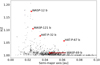 |
Fig. 10 Ratio between the substellar (X) and polar (Z) radii of planets with known properties contained in the NASA Exoplanet Archive at the time of writing (green) with the planets in Table 5 highlighted. |
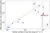 |
Fig. 11 Stellar wind mass loss rates per unit surface area in solar units as a function of the stellar surface X-ray flux for a sample of K- and G-type dwarfs (blue circles, adopted from Wood et al. 2014; Wood 2018). The dashed green line shows a power law relation of the form |

4.3 Stellar wind properties of WASP-121
The Sun loses mass at a rate of about 2 × 10⁻¹⁴ M⊙ yr−1 in the form of the solar coronal wind, which expands into space until it interacts with the surrounding interstellar medium to form the heliosphere (Wood et al. 2014). Solar-like winds of other main sequence stars can be studied using ultraviolet Lyman α line absorption produced in the astrospheres (e.g., Wood et al. 2014). In Fig. 11, we show the thus determined stellar wind mass loss rates per unit surface area, ṁ, of a sample of G- and K-type dwarf stars as a function of the respective X-ray surface fluxes, fX, presented by Wood (2018). For X-ray surface fluxes below about 106 erg cm−2 s−1 , the correlation between the quantities is well described by a power law of the form  , after which the known wind mass loss rates strongly drop, giving rise to the notion of a wind dividing line.
Instead of the interaction with the interstellar medium, interactions with an extended planetary atmosphere can also be used to study the stellar winds. A case in point is presented by Vidotto & Bourrier (2017) who use the planetary atmosphere of GJ 436 b as a probe to examine the wind of GJ 436. Along similar lines, our 3D modeling suggested that a stellar wind mass loss rate of at least 2 × 10¹³ g s−1 or 3.4 × 10⁻¹³ M⊙ yr−1 is required to shape the geometry of the planetary atmosphere of WASP-121 b. In Fig. 11, we put this value into the context of the existing sample of G- and K-type dwarfs, adopting the flux shortward of 100 Å (Sect. 2.2) to calculate the X-ray surface flux of WASP-121. Assuming that the F-type star WASP-121 fits into the same picture, we find it close to the empirical wind dividing line. The constraint on the stellar wind mass loss rate provided by our modeling is fully consistent with the alleged power law trend, which suggests even higher values.
5 Conclusion
We present high-resolution near-infrared transit spectroscopy of the hot Jupiter WASP-121 b. Our observations show a pronounced signal attributable to He I λ10833 triplet absorption in the planetary atmosphere. The maximum observed depth of the transit-averaged signal is nearly 2%. The signal is too strong to be caused by material confined to within the planetary Roche lobe, directly implying an atmosphere in the process of Roche lobe overflow. Our analysis did not provide strong evidence for a significantly prolonged He I λ10833 transit. Nonetheless, an early ingress in the planetary frame may exist along with additional absorption in the stellar rest frame.
We could appropriately reproduce the observed He I λ10833 transmission spectrum using hydrodynamic 3D modeling of the planetary atmosphere. Our results indicate asymmetric mass loss from the planet, producing a more pronounced leading tail, which may be responsible for He I λ10833 absorption signatures approximately stationary in the stellar rest frame close to the wavelength of the He I λ10833 lines. A stronger leading tail is phenomenologically consistent with the atmospheric geometries detected in HAT-P-67 b and HAT-P-32 b, all of them being likely attributable to the day- nightside asymmetry of the instel-lation. The stellar wind mass loss rates required to shape the planetary atmospheric geometry in our modeling are compatible with expectations from existing observations. While the latter comprise only stars of later spectral type, the result highlights the value of planetary atmospheres as probes into the stellar environment.
A comparison of our He I λ10833-informed estimate of the planetary mass loss rate with the prediction of the energy-limited escape formalism shows consistent results so that XUV-driven hydrodynamic atmospheric expansion appears to be a plausible mass loss mechanism in WASP-121 b. The results clearly demonstrate the importance of the He I λ10833 triplet as a diagnostic of the geometry and physics of planetary atmospheres, the capabilities of the new CRIRES+ instrument to reveal them, and the diversity of atmospheric tracers observable to study the atmosphere of WASP-121 b.
Data availability
Supplementary material is available at https://zenodo.org/records/13985969
Acknowledgements
We thank our referee Chenliang Huang for valuable comments, which helped to improve our manuscript. This work made extensive use of the Python packages PyAstronomy (Czesla et al. 2019), emcee (Foreman-Mackey et al. 2013), NumPy (Harris et al. 2020), and matplotlib (Hunter 2007). This research has made use of the NASA Exoplanet Archive, which is operated by the California Institute of Technology, under contract with the National Aeronautics and Space Administration under the Exoplanet Exploration Program. We acknowledge support through the HST program number GO-16701 and the MUSCLES collaboration members (in alphabetical order): Jacob Bean, Patrick Behr, Zachory Berta-Thompson, Alexander Brown, Girish Duvvuri, Kevin France, Cynthia Froning, Eliza Kempton, Yamila Miguel, Thomas Mikal-Evans, Sebastian Pineda, Christian Schneider, David Wilson, and Allison Youngblood. D.C. is supported by the LMU-Munich Fraunhofer-Schwarzschild Fellowship and by the Deutsche Forschungsgemeinschaft (DFG, German Research Foundation) under Germany`s Excellence Strategy – EXC 2094 – 390783311. M.R. acknowledges the support by the DFG priority program SPP 1992 “Exploring the Diversity of Extrasolar Planets” (DFG PR 36 24602/41). D.S. acknowledges financial support from the project PID2021-126365NB-C21(MCI/AEI/FEDER, UE) and from the Severo Ochoa grant CEX2021-001131-S funded by MCIN/AEI/10.13039/501100011033 S.C. acknowledges the support by the DFG priority program SPP 1992 “Exploring the Diversity of Extrasolar Planets” (DFG CZ 222/5-1). L.B.-Ch. acknowledges support by the Knut and Alice Wallenberg Foundation (grant 2018.0192) F.Y. acknowledges the support by the National Natural Science Foundation of China (grant No. 42375118). F. L. acknowledges the support by the Deutsche Forschungsgemeinschaft (DFG, German Research Foundation) - Project number 314665159. We would like to thank SURFsara (www.surfsara.nl) for their support in using the Snellius Dutch National supercomputer, as well as A. Oklopčić and M. MacLeod for their helpful discussions.
Appendix A Observation log
A.1 Wavelength correction and spectral resolution
Log of observation. Time refers to the middle of the observation (BJDTDB–2459997) and Nod denotes the nodding position.
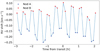 |
Fig. A.1 Shift between the wavelength solution produced by molecf it and the CRIRES+ pipeline around the He I λ10833 lines. |
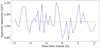 |
Fig. A.2 Spectral resolution obtained from molecfit fit along with mean value (dotted horizontal line). |
Appendix B Additional 3D modeling figures
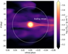 |
Fig. B.1 Projected surface density of the planetary wind as seen by the observer. The planet moves from left to right, with the leading stream being observed during negative orbital phases. The red circle represents the angular size of the planet and the white circle the angular size of the stellar disk, and thus the gas probed during mid-transit. In the leading stream, at phase -0.03, the gas converges and flares out again. In this high-density region, the gas is moving away from the observer, resulting in a redshifted spectral feature. |
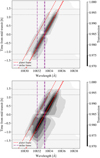 |
Fig. B.2 Synthetic spectral time series obtained from the 3D simulations. The top panel displays the spectra from the density I scenario, while the bottom panel shows the spectra from the same snapshot but using a density and pressure by a factor of 2.0 higher (density II). Purple vertical lines represent the stellar rest-frame wavelength of the metastable helium triplet in vacuum, and red tilted lines denote the planetary rest frame. Horizontal dotted lines indicate the transit contact points. The gray color map illustrates the transmission of the spectra, consistently following the planetary rest frame during the transit in both scenarios. In the higher density case (bottom), the contribution of the secondary red-shifted component becomes visible even during pre-transit phases. |
References
- Allard, F. 2016, in SF2A-2016: Proceedings of the Annual meeting of the French Society of Astronomy and Astrophysics, eds. C. Reylé, J. Richard, L. Cambrésy, M. Deleuil, E. Pécontal, L. Tresse, & I. Vauglin, 223 [Google Scholar]
- Azevedo Silva, T., Demangeon, O. D. S., Santos, N. C., et al. 2022, A&A, 666, L10 [NASA ADS] [CrossRef] [EDP Sciences] [Google Scholar]
- Boldt-Christmas, L., Lesjak, F., Wehrhahn, A., et al. 2024, A&A, 683, A244 [NASA ADS] [CrossRef] [EDP Sciences] [Google Scholar]
- Borsa, F., Allart, R., Casasayas-Barris, N., et al. 2021, A&A, 645, A24 [EDP Sciences] [Google Scholar]
- Bourrier, V., Ehrenreich, D., Lendl, M., et al. 2020, A&A, 635, A205 [NASA ADS] [CrossRef] [EDP Sciences] [Google Scholar]
- Changeat, Q., Skinner, J. W., Cho, J. Y. K., et al. 2024, ApJS, 270, 34 [NASA ADS] [CrossRef] [Google Scholar]
- Claret, A., Diaz-Cordoves, J., & Gimenez, A. 1995, A&AS, 114, 247 [NASA ADS] [Google Scholar]
- Cruz Aguirre, F., France, K., Nell, N., et al. 2023, ApJ, 956, 79 [NASA ADS] [CrossRef] [Google Scholar]
- Czesla, S., Klocová, T., Khalafinejad, S., Wolter, U., & Schmitt, J. H. M. M. 2015, A&A, 582, A51 [NASA ADS] [CrossRef] [EDP Sciences] [Google Scholar]
- Czesla, S., Schröter, S., Schneider, C. P., et al. 2019, PyA: Python astronomy-related packages, Astrophysics Source Code Library [record ascl:1906.010] [Google Scholar]
- Czesla, S., Lampón, M., Sanz-Forcada, J., et al. 2022, A&A, 657, A6 [NASA ADS] [CrossRef] [EDP Sciences] [Google Scholar]
- Czesla, S., Lampón, M., Cont, D., et al. 2024, A&A, 683, A67 [NASA ADS] [CrossRef] [EDP Sciences] [Google Scholar]
- Delrez, L., Santerne, A., Almenara, J. M., et al. 2016, MNRAS, 458, 4025 [NASA ADS] [CrossRef] [Google Scholar]
- Dorn, R. J., Bristow, P., Smoker, J. V., et al. 2023, A&A, 671, A24 [NASA ADS] [CrossRef] [EDP Sciences] [Google Scholar]
- Duvvuri, G. M., Pineda, J. S., Berta-Thompson, Z. K., et al. 2021, ApJ, 913, 40 [NASA ADS] [CrossRef] [Google Scholar]
- Erkaev, N. V., Kulikov, Y. N., Lammer, H., et al. 2007, A&A, 472, 329 [NASA ADS] [CrossRef] [EDP Sciences] [Google Scholar]
- Evans, T. M., Sing, D. K., Goyal, J. M., et al. 2018, AJ, 156, 283 [NASA ADS] [CrossRef] [Google Scholar]
- Foreman-Mackey, D., Hogg, D. W., Lang, D., & Goodman, J. 2013, PASP, 125, 306 [Google Scholar]
- Fossati, L., Ayres, T. R., Haswell, C. A., et al. 2013, ApJ, 766, L20 [Google Scholar]
- Fu, G., Espinoza, N., Sing, D. K., et al. 2022, ApJ, 940, L35 [NASA ADS] [CrossRef] [Google Scholar]
- Fuhrmeister, B., Czesla, S., Hildebrandt, L., et al. 2019, A&A, 632, A24 [NASA ADS] [CrossRef] [EDP Sciences] [Google Scholar]
- Gaia Collaboration (Vallenari, A., et al.) 2023, A&A, 674, A1 [NASA ADS] [CrossRef] [EDP Sciences] [Google Scholar]
- Gibson, N. P., Nugroho, S. K., Lothringer, J., Maguire, C., & Sing, D. K. 2022, MNRAS, 512, 4618 [NASA ADS] [CrossRef] [Google Scholar]
- Gully-Santiago, M., Morley, C. V., Luna, J., et al. 2024, AJ, 167, 142 [NASA ADS] [CrossRef] [Google Scholar]
- Harris, C. R., Millman, K. J., van der Walt, S. J., et al. 2020, Nature, 585, 357 [NASA ADS] [CrossRef] [Google Scholar]
- Haswell, C. A., Fossati, L., Ayres, T., et al. 2012, ApJ, 760, 79 [Google Scholar]
- Hoeijmakers, H. J., Seidel, J. V., Pino, L., et al. 2020, A&A, 641, A123 [NASA ADS] [CrossRef] [EDP Sciences] [Google Scholar]
- Hoeijmakers, H. J., Kitzmann, D., Morris, B. M., et al. 2024, A&A, 685, A139 [NASA ADS] [CrossRef] [EDP Sciences] [Google Scholar]
- Huang, C., Koskinen, T., Lavvas, P., & Fossati, L. 2023, ApJ, 951, 123 [NASA ADS] [CrossRef] [Google Scholar]
- Hunter, J. D. 2007, Comput. Sci. Eng., 9, 90 [NASA ADS] [CrossRef] [Google Scholar]
- Husser, T.-O., Wende-von Berg, S., Dreizler, S., et al. 2013, A&A, 553, A6 [NASA ADS] [CrossRef] [EDP Sciences] [Google Scholar]
- Jeffreys, H. 1932, Proc. Roy. Soc. Lond. Ser. A, 138, 48 [NASA ADS] [CrossRef] [Google Scholar]
- Jensen, A. G., Cauley, P. W., Redfield, S., Cochran, W. D., & Endl, M. 2018, AJ, 156, 154 [Google Scholar]
- Kass, R. E., & Raftery, A. E. 1995, J. Am. Statist. Assoc., 90, 773 [CrossRef] [Google Scholar]
- Kausch, W., Noll, S., Smette, A., et al. 2015, A&A, 576, A78 [NASA ADS] [CrossRef] [EDP Sciences] [Google Scholar]
- Koskinen, T. T., Lavvas, P., Huang, C., et al. 2022, ApJ, 929, 52 [NASA ADS] [CrossRef] [Google Scholar]
- Lammer, H., Selsis, F., Ribas, I., et al. 2003, ApJ, 598, L121 [Google Scholar]
- Lampón, M., López-Puertas, M., Sanz-Forcada, J., et al. 2023, A&A, 673, A140 [NASA ADS] [CrossRef] [EDP Sciences] [Google Scholar]
- Li, S.-L., Miller, N., Lin, D. N. C., & Fortney, J. J. 2010, Nature, 463, 1054 [NASA ADS] [CrossRef] [Google Scholar]
- Loyd, R. O. P., France, K., Youngblood, A., et al. 2016, ApJ, 824, 102 [NASA ADS] [CrossRef] [Google Scholar]
- MacLeod, M., & Oklopcic, A. 2022, ApJ, 926, 226 [NASA ADS] [CrossRef] [Google Scholar]
- Maguire, C., Gibson, N. P., Nugroho, S. K., et al. 2023, MNRAS, 519, 1030 [Google Scholar]
- Mandel, K., & Agol, E. 2002, ApJ, 580, L171 [Google Scholar]
- Merritt, S. R., Gibson, N. P., Nugroho, S. K., et al. 2021, MNRAS, 506, 3853 [NASA ADS] [CrossRef] [Google Scholar]
- Mikal-Evans, T., Sing, D. K., Barstow, J. K., et al. 2022, Nat. Astron., 6, 471 [NASA ADS] [CrossRef] [Google Scholar]
- Mikal-Evans, T., Sing, D. K., Dong, J., et al. 2023, ApJ, 943, L17 [CrossRef] [Google Scholar]
- Morello, G., Changeat, Q., Dyrek, A., Lagage, P. O., & Tan, J. C. 2023, A&A, 676, A54 [NASA ADS] [CrossRef] [EDP Sciences] [Google Scholar]
- Murray-Clay, R. A., Chiang, E. I., & Murray, N. 2009, ApJ, 693, 23 [Google Scholar]
- Nail, F., MacLeod, M., Oklopcic, A., et al. 2024a, A&A, submitted [arXiv:2410.19381] [Google Scholar]
- Nail, F., Oklcpcic, A., & MacLeod, M. 2024b, A&A, 684, A20 [NASA ADS] [CrossRef] [EDP Sciences] [Google Scholar]
- Nortmann, L., Pallé, E., Salz, M., et al. 2018, Science, 362, 1388 [Google Scholar]
- Ouyang, Q., Wang, W., Zhai, M., et al. 2023, Res. Astron. Astrophys., 23, 065010 [CrossRef] [Google Scholar]
- Pizzocaro, D., Stelzer, B., Poretti, E., et al. 2019, A&A, 628, A41 [NASA ADS] [CrossRef] [EDP Sciences] [Google Scholar]
- Powell, M. J. D. 1964, Comput. J., 7, 155 [Google Scholar]
- Salz, M., Schneider, P. C., Czesla, S., & Schmitt, J. H. M. M. 2016, A&A, 585, L2 [NASA ADS] [CrossRef] [EDP Sciences] [Google Scholar]
- Salz, M., Czesla, S., Schneider, P. C., et al. 2018, A&A, 620, A97 [NASA ADS] [CrossRef] [EDP Sciences] [Google Scholar]
- Salz, M., Schneider, P. C., Fossati, L., et al. 2019, A&A, 623, A57 [NASA ADS] [CrossRef] [EDP Sciences] [Google Scholar]
- Sanz-Forcada, J., & Dupree, A. K. 2008, A&A, 488, 715 [NASA ADS] [CrossRef] [EDP Sciences] [Google Scholar]
- Sanz-Forcada, J., Micela, G., Ribas, I., et al. 2011, A&A, 532, A6 [NASA ADS] [CrossRef] [EDP Sciences] [Google Scholar]
- Seidel, J. V., Borsa, F., Pino, L., et al. 2023, A&A, 673, A125 [NASA ADS] [CrossRef] [EDP Sciences] [Google Scholar]
- Sharma, S. 2017, ARA&A, 55, 213 [Google Scholar]
- Sing, D. K., Lavvas, P., Ballester, G. E., et al. 2019, AJ, 158, 91 [Google Scholar]
- Smette, A., Sana, H., Noll, S., et al. 2015, A&A, 576, A77 [NASA ADS] [CrossRef] [EDP Sciences] [Google Scholar]
- Smith, R. K., Brickhouse, N. S., Liedahl, D. A., & Raymond, J. C. 2001, ApJ, 556, L91 [Google Scholar]
- Spake, J. J., Oklopcic, A., & Hillenbrand, L. A. 2021, AJ, 162, 284 [NASA ADS] [CrossRef] [Google Scholar]
- Stone, J. M., Tomida, K., White, C. J., & Felker, K. G. 2020, ApJS, 249, 4 [NASA ADS] [CrossRef] [Google Scholar]
- Tyler, D., Petigura, E. A., Oklopcic, A., & David, T. J. 2024, ApJ, 960, 123 [NASA ADS] [CrossRef] [Google Scholar]
- Vidotto, A. A., & Bourrier, V. 2017, MNRAS, 470, 4026 [NASA ADS] [CrossRef] [Google Scholar]
- Wang, L., & Dai, F. 2021, ApJ, 914, 98 [NASA ADS] [CrossRef] [Google Scholar]
- Watson, A. J., Donahue, T. M., & Walker, J. C. G. 1981, Icarus, 48, 150 [NASA ADS] [CrossRef] [Google Scholar]
- Wilson, J., Gibson, N. P., Lothringer, J. D., et al. 2021, MNRAS, 503, 4787 [NASA ADS] [CrossRef] [Google Scholar]
- Wood, B. E. 2018, in Journal of Physics Conference Series, 1100, 012028 [NASA ADS] [CrossRef] [Google Scholar]
- Wood, B. E., Müller, H.-R., Redfield, S., & Edelman, E. 2014, ApJ, 781, L33 [Google Scholar]
- Yan, F., Fosbury, R. A. E., Petr-Gotzens, M. G., Zhao, G., & Pallé, E. 2015, A&A, 574, A94 [NASA ADS] [CrossRef] [EDP Sciences] [Google Scholar]
- Yan, D., Guo, J., Huang, C., & Xing, L. 2021, ApJ, 907, L47 [NASA ADS] [CrossRef] [Google Scholar]
- Yan, F., Nortmann, L., Reiners, A., et al. 2023, A&A, 672, A107 [NASA ADS] [CrossRef] [EDP Sciences] [Google Scholar]
- Zhang, Z., Morley, C. V., Gully-Santiago, M., et al. 2023, Sci. Adv., 9, eadf8736 [Google Scholar]
Delrez et al. (2016) apparently used the mean radius of Jupiter as length unit, while we use the equatorial radius.
All Tables
Stellar luminosities of WASP-121 and fluxes at the planetary orbital separation of WASP-121 b for various spectral bands.
Line characteristics as well as the planetary and stellar mass loss rates obtained from the three-dimensional modeling.
Log of observation. Time refers to the middle of the observation (BJDTDB–2459997) and Nod denotes the nodding position.
All Figures
|
Fig. 1 Mean S/N per spectral bin (blue squares) in the 10 830–10 840 Å range and the airmass (red circles) for the spectral time series. Vertical dotted lines indicate the optical first to fourth contact. |
| In the text | |
|
Fig. 2 Spectra energy distribution of WASP-121, with the sources of each wavelength region labeled at the top. The SED is compared with that of the Sun scaled to the same bolometric luminosity. |
| In the text | |
|
Fig. 3 Out-of-transit master spectrum of WASP-121 around the He I λ10833 triplet lines in the stellar rest frame (blue) along with synthetic model (red). The wavelengths of the He I λ10833 triplet lines are indicated by dotted green lines. |
| In the text | |
|
Fig. 4 Maps of transmission spectra and residuals (smoothed) of the He I λ10833 region in the stellar reference frame. The top panel shows the observed transmission spectra and the bottom panel the residuals after subtraction of the best-fit model (color coded). The horizontal lines (black dashed) indicate the optical first to fourth contact times, dotted yellow lines (vertical) show the location of the telluric OH line components, the dash-dotted magenta line indicates the wavelength of the stellar He I λ10833 line, and the dashed red line (diagonal) shows the radial velocity track of the planetary orbit. |
| In the text | |
|
Fig. 5 Time evolution of He I λ10833 transmission. The temporal evolution of the shape parameters (top panel) and the narrow-band, ±0.25 Å He I λ10833 transmission light curve in the bottom panel. Solid lines indicate transit models for an annulus-shaped atmosphere with various outer radii and the vertical dotted lines mark the optical contact point. |
| In the text | |
|
Fig. 6 Light curve extracted from a ±0.5 Å region around the rest wavelength of the He I λ10833 line before (solid red) and after (dashed blue) subtraction of the best-fit empirical model. |
| In the text | |
|
Fig. 7 Averaged transmission spectrum between optical second and third contact. The red lines show three best-fit empirical models with 5% filling factor and one (dashed) and two (solid) absorbing components. The vertical dotted lines show the wavelengths of the He I λ10833 triplet lines. |
| In the text | |
|
Fig. 8 Simulated metastable helium number density (top) and the line-oſ-sight velocity (bottom) in the orbital mid-plane of the WASP-121 system. The host star, located at the coordinate origin, is orbited by the planet, located on the negative x-axis, in counterclockwise direction. The observer is also located on the negative x-axis. The bottom panel shows the velocity component in the x-direction, representing the observer’s view during mid-transit. Purple and white contours indicate the cumulative optical depth at the center of the He I λ10833 line, with τ = 10 and τ = 1, respectively; solid and dotted contours represent the density I and II setup. The planetary outflow forms a red-shifted, leading tail, which originates from the more pronounced day side outflow. |
| In the text | |
|
Fig. 9 Synthetic transmission spectra derived from our 3D simulation for the density I (red solid line) and density II (blue solid line) setups. As for the underlying observations (gray), a time average between the optical second and third transit contact is displayed. The shaded regions represent the range of model transmission spectra obtained during the transit. The synthetic spectra are multiplied by a factor of 1.00191 (Sect. 3.4.4) to match the observational continuum. The red solid line aligns well with the observed helium triplet, while the location of the secondary red component can be reproduced by considering a higher density of the same outflow structure. |
| In the text | |
|
Fig. 10 Ratio between the substellar (X) and polar (Z) radii of planets with known properties contained in the NASA Exoplanet Archive at the time of writing (green) with the planets in Table 5 highlighted. |
| In the text | |
|
Fig. 11 Stellar wind mass loss rates per unit surface area in solar units as a function of the stellar surface X-ray flux for a sample of K- and G-type dwarfs (blue circles, adopted from Wood et al. 2014; Wood 2018). The dashed green line shows a power law relation of the form |
| In the text | |
|
Fig. A.1 Shift between the wavelength solution produced by molecf it and the CRIRES+ pipeline around the He I λ10833 lines. |
| In the text | |
|
Fig. A.2 Spectral resolution obtained from molecfit fit along with mean value (dotted horizontal line). |
| In the text | |
|
Fig. B.1 Projected surface density of the planetary wind as seen by the observer. The planet moves from left to right, with the leading stream being observed during negative orbital phases. The red circle represents the angular size of the planet and the white circle the angular size of the stellar disk, and thus the gas probed during mid-transit. In the leading stream, at phase -0.03, the gas converges and flares out again. In this high-density region, the gas is moving away from the observer, resulting in a redshifted spectral feature. |
| In the text | |
|
Fig. B.2 Synthetic spectral time series obtained from the 3D simulations. The top panel displays the spectra from the density I scenario, while the bottom panel shows the spectra from the same snapshot but using a density and pressure by a factor of 2.0 higher (density II). Purple vertical lines represent the stellar rest-frame wavelength of the metastable helium triplet in vacuum, and red tilted lines denote the planetary rest frame. Horizontal dotted lines indicate the transit contact points. The gray color map illustrates the transmission of the spectra, consistently following the planetary rest frame during the transit in both scenarios. In the higher density case (bottom), the contribution of the secondary red-shifted component becomes visible even during pre-transit phases. |
| In the text | |
Current usage metrics show cumulative count of Article Views (full-text article views including HTML views, PDF and ePub downloads, according to the available data) and Abstracts Views on Vision4Press platform.
Data correspond to usage on the plateform after 2015. The current usage metrics is available 48-96 hours after online publication and is updated daily on week days.
Initial download of the metrics may take a while.