| Issue |
A&A
Volume 686, June 2024
|
|
|---|---|---|
| Article Number | A208 | |
| Number of page(s) | 13 | |
| Section | Planets and planetary systems | |
| DOI | https://doi.org/10.1051/0004-6361/202348210 | |
| Published online | 13 June 2024 | |
A possibly solar metallicity atmosphere escaping from HAT-P-32b revealed by Hα and He absorption
1
Yunnan Observatories, Chinese Academy of Sciences,
PO Box 110,
Kunming
650216,
PR
China
e-mail: This email address is being protected from spambots. You need JavaScript enabled to view it.
2
Key Laboratory for the Structure and Evolution of Celestial Objects, CAS,
Kunming
650216,
PR
China
3
International Centre of Supernovae, Yunnan Key Laboratory,
Kunming
650216,
PR
China
4
School of Astronomy and Space Science, University of Chinese Academy of Sciences,
Beijing,
PR
China
5
Korea Astronomy & Space Science Institute,
776 Daedeokdae-ro, Yuseong-gu,
Daejeon
34055,
Republic of Korea
6
Astronomy and Space Science Major, University of Science and Technology,
217, Gajeong-ro, Yuseong-gu,
Daejeon
34113,
Republic of Korea
7
Instituto de Astrofísica de Andalucía (IAA-CSIC), Glorieta de la Astronomía s/n,
18008
Granada,
Spain
8
Thüringer Landessternwarte Tautenburg,
Sternwarte 5,
07778
Tautenburg,
Germany
Received:
9
October
2023
Accepted:
25
March
2024
Abstract
This paper presents a hydrodynamic simulation that couples detailed non-local thermodynamic equilibrium (NLTE) calculations of the helium and hydrogen level populations to model the Hα and He 10830 transmission spectra of the hot Jupiter HAT-P-32b. A Monte Carlo simulation was applied to calculate the number of Lyα resonance scatterings, which is the main process for populating H(2). In the examined parameter space, only models with H/He ≥ 99.5/0.5, (0.5 ~ 3.0) times the fiducial value of FXUV, and spectral index βm = (0.16 ~ 0.3), can explain the Hα and He 10830 lines simultaneously. We found a mass-loss rate of ~(1.0 ~ 3.1) × 1013 g s−1, consistent with previous studies. Moreover, we found that the stellar Lyα flux should be as high as 4 × 10⁵ erg cm−2 s−1, indicating high stellar activity during the observation epoch of the two absorption lines. Despite the fact that the metallicity in the lower atmosphere of HAT-P-32b may be super-solar, our simulations tentatively suggest it is close to solar in the upper atmosphere. Understanding the difference in metallicity between the lower and upper atmospheres is essential for future atmospheric characterisations.
Key words: hydrodynamics / radiative transfer / methods: numerical / planets and satellites: atmospheres / planets and satellites: composition / planets and satellites: individual: HAT-P-32b
© The Authors 2024
 Open Access article, published by EDP Sciences, under the terms of the Creative Commons Attribution License (https://creativecommons.org/licenses/by/4.0), which permits unrestricted use, distribution, and reproduction in any medium, provided the original work is properly cited.
This article is published in open access under the Subscribe to Open model. This email address is being protected from spambots. You need JavaScript enabled to view it. to support open access publication.
1 Introduction
Hydrogen and helium are the two most abundant elements in the atmospheres of giant planets both in solar and extrasolar systems. Over the past two decades, the escaping atmospheres of hydrogen and helium have been detected by the excess absorption lines through transmission spectroscopy. To detect hydrogen during transit, the Lyα line in the ultraviolet has been initially employed because of its high absorption depth caused by the predominant presence of hydrogen in the ground state H(1s) (Vidal-Madjar et al. 2003; Lecavelier Des Etangs et al. 2010, 2012; Kulow et al. 2014; Ehrenreich et al. 2015; Bourrier et al. 2018; Ben-Jaffel et al. 2022; Zhang et al. 2022c). As a complementary information, the Hα line in the optical is able to probe planetary hydrogen atoms in the excited state, H(2) (Jensen et al. 2012, 2018; Yan & Henning 2018; Yan et al. 2021b; Casasayas-Barris et al. 2018; Cauley et al. 2019, 2021; Cabot et al. 2020; Chen et al. 2020; Borsa et al. 2021; Czesla et al. 2022). To detect helium, its infrared triplet (hereafter, He 10830), which arises from the transition between 23S and 23P state, is utilised. Excess absorption of He 10830 by the planet’s atmosphere during transit is a signature of the existence of metastable helium H(23S) (Seager & Sasselov 2000; Oklopčić & Hirata 2018; Spake et al. 2018; Salz et al. 2018; Nortmann et al. 2018; Allart et al. 2018; Alonso-Floriano et al. 2019; Kirk et al. 2022; Zhang et al. 2022b, 2023a,b). Because both the Hα and He 10830 lines are not contaminated by interstellar absorption and can be observed by ground-based telescopes with large apertures and high spectral resolutions, it is common to use them to probe hydrogen and helium in planetary atmospheres.
The excess absorptions of both the Hα and He 10830 lines have been detected only in four systems, namely, HD 189733b (Jensen et al. 2012; Barnes et al. 2016; Cauley et al. 2017; Salz et al. 2018; Guilluy et al. 2020; Zhang et al. 2022a; Allart et al. 2023), WASP-52b (Chen et al. 2020; Vissapragada et al. 2020, 2022; Kirk et al. 2022; Allart et al. 2023), HAT-P-32b (Czesla et al. 2022; Zhang et al. 2023b), and HAT-P-67b (Bello-Arufe et al. 2023; Gully-Santiago et al. 2023). Simultaneously modelling the transmission spectra of Hα and He 10830 lines can help to constrain the physical parameters of the planetary atmosphere. In particular, the mass-loss rate of exoplanets with an expanding atmosphere has been found to be as high as 109−1013 g s−1 (Guo 2011, 2013; Salz et al. 2016; Khodachenko et al. 2021; Koskinen et al. 2022); such a high mass-loss rate could play a crucial role in planetary compositions and dynamics and especially in the evolutions and architectures (e.g. occurrence) of small-sized exoplanets (Fulton & Petigura 2018; Owen & Lai 2018; Yee et al. 2020; Vissapragada et al. 2022; Lampón et al. 2023). The energy-limited approach allows us to estimate the planetary mass-loss rate based on the absorbed energy (Lammer et al. 2003; Erkaev et al. 2007). However, for planets with very high gravitational potentials or those exposed to intense X-ray and extreme ultraviolet (XUV) flux, this approach can yield a mass-loss rate significantly different from that obtained using more complex, self-consistent models (Salz et al. 2016; Yang & Guo 2019; Lampón et al. 2021a; Caldiroli et al. 2021). Moreover, the energy-limited approach cannot provide detailed atmospheric structures that are necessary to interpret the transmission signals. Therefore, a self-consistent hydrodynamic calculation is essential for analysing the observations and gaining information about the escaping atmosphere.
In atmospheric modelling, some physical parameters or quantities are challenging to measure or estimate. For example, the XUV (1–912 Å) radiation from host stars, which plays an essential role in the heating and photochemistry of the planetary atmosphere, is difficult to measure because the extreme ultraviolet (EUV) radiation is readily absorbed by the interstellar medium (ISM). There are some works to reconstruct the XUV spectra. For instance, the MUSCLES Treasury Survey is dedicated to reconstruct the spectral energy distributions (SEDs) of M- and K-type stars in a range of 5 Å to 5.5 micron, including the XUV band (France et al. 2016). The X-ray spectra of these stars can be detected using the Chandra X-ray Observatory and XMM-Newton instruments or simulated using the APEC models (Smith et al. 2001). The EUV spectra are obtained by using either the empirical scaling relation based on Lyα flux (Linsky et al. 2014), with the Lyα spectra reconstructed from model fits that take the stellar flux and interstellar medium into account (Youngblood et al. 2016), or through the use of the differential emission measure models (Duvvuri et al. 2021). For the late-type stars, Sanz-Forcada et al. (2011) derived a relation between the X-ray and EUV flux, and both of these can be estimated for a given stellar age. A few works obtain the SEDs by using the XSPEC software (Arnaud 1996). However, despite employing these various methods, obtaining detailed XUV SEDs remains challenging. All the reconstructed XUV spectra of extrasolar systems are rather uncertain, both in flux and in spectral shape. While the He 10830 absorption is sensitive to the XUV flux (Yan et al. 2022), these order-of-magnitude uncertainties on the XUV spectra do not necessarily translate to order-of-magnitude uncertainties on the absorption signatures, as suggested by Linssen et al. (2022). Modelling the observed transmission spectral lines can help constrain the XUV radiation (Yan et al. 2021a, 2022). In addition, the hydrogen-to-helium abundance ratio, H/He, may be significantly different from that of the Sun. By modelling the He 10830 transmission spectra of some exoplanets, it was found that a much higher H/He, or equivalently a much lower helium abundance, is estimated in the planetary upper atmosphere (Lampón et al. 2020, 2021b, 2023; Shaikhislamov et al. 2021; Yan et al. 2022; Rumenskikh et al. 2022; Fossati et al. 2022). We consider the reasons why this is happening, for instance: whether it is harder for helium to escape, compared to hydrogen, or whether the origin of helium is different on this planet from its origin in the Sun. More detailed studies of the escaping helium atmosphere are required to explore such questions.
The first work that could explain both the Hα and He 10830 transmission spectra in an exoplanet system was carried out by Czesla et al. (2022), who used two independent models to interpret the Hα and He 10830 signals of HAT-P-32b. In the Yan et al. (2022; hereafter Paper I), we simultaneously modelled the Hα and He 10830 absorption of WASP-52b and fit the observation quite well by using a hydrodynamic model coupled with a non-local thermodynamic (NLTE) model. To calculate the H(2) population, we performed a Monte Carlo simulation and calculated the Lyα intensity inside the planetary atmosphere. The model that reproduced both lines could constrain the XUV flux (FXUV) and SEDs, as well as the hydrogen-to-helium abundance ratio H/He; finally, it could help estimate the mass-loss rate of the planet. In that work, the stellar Lyα photons were the main source to populate H(2), while the Lyα photons produced in the planetary atmosphere were negligible. Thus, we consider whether this result is universal. To answer this question, it is worthwhile analysing more systems.
Using the CARMENES spectrograph, Czesla et al. (2022) detected pronounced, time-dependent absorption in the Hα and He 10830 triplet lines with maximum depths of about 3.3% and 5.3%, respectively. These authors attributed these absorptions to the planetary atmosphere. In addition, an early ingress of redshifted absorption was observed in both lines. Czesla et al. (2022) performed pioneering work on modelling the absorption spectra of Hα and He 10830 of HAT-P-32b. To explain the Hα transmission spectrum, they used a 1D hydrodynamic model including a non-local thermodynamic equilibrium (NLTE) treatment of hydrogen level populations, using the model of García Muñoz & Schneider (2019). Their model only considers the species of hydrogen and electrons. To estimate the XUV heating, they assumed that the XUV flux received at the sub-stellar point represents the flux illuminated across the whole planetary surface. The mass-loss rate is estimated by πρur2 to account for the average effect of stellar heating, where ρ is the density of the atmosphere, u is the velocity, and r is the distance from the planetary center. In their work, the H(2) population that causes the Hα absorption, is formed in a narrow layer around 1.8RP. To model the He 10830 transmission spectrum, Czesla et al. (2022) used a variation of the 1D isothermal Parker wind model (see Lampón et al. 2020), which assumes a constant speed of sound. In contrast to that of García Muñoz & Schneider (2019), this model takes into account both hydrogen and helium. In the model, the temperature, hydrogen-to-helium abundance ratio, H/He, and mass-loss rate are free parameters. By comparing the model transmission spectrum of He 10830 with the observation, they found that H/He can be either 90/10 or 99/1. A mass-loss rate of about 1013 g s−1 was obtained by modelling the Hα and He 10830 lines in Czesla et al. (2022). Recently, Lampón et al. (2023) reanalysed the upper atmosphere of HAT-P-32b, and showed that this planet undergoes photoevaporation at a mass-loss rate of about (1.30±0.7)x1013 g s−1 and the atmosphere temperature is in the range of 12400±2900 K. They also constrained the H/He ratio in the planetary upper atmosphere to be about 99/1.
Recently, using high-resolution spectroscopy of He 10830 obtained from the Hobby–Eberly Telescope, Zhang et al. (2023b) detected the escaping helium associated with giant tidal tails of HAT-P-32b. The He 10830 absorption depth at mid-transit was ~8.2%, about 1.5 times higher than that observed by Czesla et al. (2022). The variability of He 10830 absorption in HAT-P-32b may imply a variation of stellar activity of HAT-P-32. To explain the asymmetric signals, Zhang et al. (2023b) used a 3D hydrodynamic simulation and predicted the Roche lobe overflow with extended tails. They estimated a mass-loss rate of about 1.07×10¹² g s−1, which is about an order of magnitude lower than the results of Czesla et al. (2022) and Lampón et al. (2023; see Sect. 4.3).
We note that Czesla et al. (2022) analysed the Hα and He 10830 transmission spectra separately with two independent models. In this paper, we intend to simultaneously model the Hα and He 10830 transmission spectra of HAT-P-32b using a self-consistent model for characterising its upper atmosphere. Since both the Hα and He 10830 absorptions were detected at the same time in Czesla et al. (2022), we mainly compare our model with their observation. In addition, we also discuss the He 10830 observation by Zhang et al. (2023b). Unlike the models used by Czesla et al. (2022), we simulate Lyα resonance scattering by assuming that both the stellar and planetary atmospheres are spherical. In addition, to calculate the population of He(23S), we use the atmospheric structure obtained from a non-isothermal hydrodynamic model. Hence, this work presents an important modelling effort to understand the atmospheric outflow of HAT-P-32b and provides additional constrains on its upper atmosphere.
The paper is organised as follows. In Sec. 2, we describe the method. Section 3 compares the results with observations and other modelling works. In Sect. 4, we discuss some relevant subjects to the present work, including the escape of helium. Finally, Sec. 5 summarises our work and presents our conclusions.
Parameters and model settings.
2 Method
We used a 1D hydrodynamic model (Guo & Ben-Jaffel 2016; Yang & Guo 2018, 2019) to simulate the atmospheric structure of HAT-P-32b and to obtain the atmospheric temperature, velocity, and particle number densities. The planetary and stellar parameters are based on reported observations (Hartman et al. 2011; Czesla et al. 2022). HAT-P-32 is an F-type star with M* = 1.160 M⊙ and R* = 1.219 R⊙, while HAT-P-32b is a hot Jupiter with MP = 0.585 MJ and RP = 1.789RJ. The equilibrium temperature is 1805 K, which is adopted as the temperature at the lower boundary in our model. The integrated flux in the XUV band is a crucial parameter in the simulations. Here, we adopted the spectral energy distribution (SED) up to 920 Å and the luminosity in the ranges of 100–504 Å and 100–920 Å of Czesla et al. (2022), which are based on XMM-Newton X-ray observations. The fluxes in each band along with other model parameters are presented in Table 1. Using the SED, the total XUV flux is estimated to be about FXUV = 4.2 × 10⁵ erg cm−2 s−1 (hereafter F0, the fiducial XUV flux) at the planetary orbit (0.0343 AU). We note that this value is at the sub-stellar point and there is no flux on the nightside for the 1D model. Therefore, in our calculation, this value is divided by a factor of 4, which accounts for the uniform redistribution of the stellar radiation energy around the planet. The SED index, βm = F(1–100 Å)/F(1–912 Å), as defined in Yan et al. (2021a), is about 0.16. We reconstructed the SEDs in the FUV and NUV (912–3646 Å) wavelengths based on the stellar atmosphere model of Castelli & Kurucz (2003). The stellar XUV, FUV, and NUV SEDs are shown in Fig. 1.
The chemical composition of HAT-P-32b is initially assumed to be the same as that of HAT-P-32, which is identical to the solar abundances except for [Fe/H] = −0.04. This can lead to a slight change in the atmospheric scale height compared to using solar metallicity. In this study, we have not included the cooling effects caused by metals (C, N, O, Si, and their respective ions). Cooling by metals such as Fe II or Mg II can be significant under certain circumstances (Zhang et al. 2022b; Huang et al. 2023). For example, Zhang et al. (2022b) found that Fe II compromises 30% of the cooling from (1.6–2.0) RP and (2.9–3.4) RP in the atmosphere with a solar metallicity of TOI 560.01, but cooling by hydrogen is still dominant; for a higher metallicity, the cooling of metals becomes more important. Huang et al. (2023) found that cooling by Mg II in the atmosphere of WASP-121b can be dominant at altitudes lower than ~1.4 RP. However, these metals are not included in our model, thus their cooling effects are not considered and we defer such studies to a future work.
Initially, we assumed a number ratio of hydrogen to helium to be the same as the solar value (H/He = 92/8, Asplund et al. 2009). We then explored the effects of varying the H/He ratio while maintaining constant metallicity. We note that while the stellar metallicity is almost solar, the planetary atmosphere may have a different metallicity. Transmission spectroscopy of the lower atmosphere conducted with Hubble Space Telescope and Spitzer Infrared Array Camera photometry has suggested that the atmosphere of HAT-P-32b is metal-rich, with a metallicity of likely exceeding 100 (or 200) times the solar value, that is: ![Mathematical equation: $\[\log \left(Z / Z_{\odot}\right)=2.41_{-0.07}^{+0.06}\]$](/articles/aa/full_html/2024/06/aa48210-23/aa48210-23-eq6.png) (Alam et al. 2020). However, the upper atmosphere remains unclear whether such a high metallicity could appear, as heavy species may not escape as easily as the light ones. Multi-fluid hydrodynamic simulations have shown that the decoupling of heavy and light species can occur when collisions between them become less frequent. In such cases, the heavy species would tend to remain in the lower atmosphere, while light ones rise to the upper atmosphere and eventually escape (Guo 2019; Xing et al. 2023). In this work, to investigate the influence of metallicity, we examined the cases of Z = 1, 10, 30, 50, 100, 200, and 300 times solar metallicity, following the convention of Zhang et al. (2022b). We note that for the case of the solar metallicity (Z = 1), the planetary atmosphere consists of 73.80% hydrogen, 24.85% helium, and 1.34% metals by mass (Asplund et al. 2009). We assume an iron abundance of [Fe/H] = −0.04 in the Z = 1 case. The mass fractions of H, He, and metals are 31.72%, 10.68%, and 57.6% for Z = 100, respectively, and 14.74%, 4.96%, and 80.30% for Z = 300. In our fiducial models (see Table 1 for details) with Z > 1, the hydrogen-to-helium abundance ratio remains 92/8. For 10 < Z < 50, only the fiducial models are considered. We calculated only a few models by varying other parameters (FXUV and βm) for each metallicity when Z > 100 because of the computational expense.
(Alam et al. 2020). However, the upper atmosphere remains unclear whether such a high metallicity could appear, as heavy species may not escape as easily as the light ones. Multi-fluid hydrodynamic simulations have shown that the decoupling of heavy and light species can occur when collisions between them become less frequent. In such cases, the heavy species would tend to remain in the lower atmosphere, while light ones rise to the upper atmosphere and eventually escape (Guo 2019; Xing et al. 2023). In this work, to investigate the influence of metallicity, we examined the cases of Z = 1, 10, 30, 50, 100, 200, and 300 times solar metallicity, following the convention of Zhang et al. (2022b). We note that for the case of the solar metallicity (Z = 1), the planetary atmosphere consists of 73.80% hydrogen, 24.85% helium, and 1.34% metals by mass (Asplund et al. 2009). We assume an iron abundance of [Fe/H] = −0.04 in the Z = 1 case. The mass fractions of H, He, and metals are 31.72%, 10.68%, and 57.6% for Z = 100, respectively, and 14.74%, 4.96%, and 80.30% for Z = 300. In our fiducial models (see Table 1 for details) with Z > 1, the hydrogen-to-helium abundance ratio remains 92/8. For 10 < Z < 50, only the fiducial models are considered. We calculated only a few models by varying other parameters (FXUV and βm) for each metallicity when Z > 100 because of the computational expense.
In the simulations, the pressure at the lower boundary (1 RP) is 1 μbar. The upper boundary is 10 RP, which is larger than the radius of the host star (about 6.7 RP). The Lyα cooling and stellar tidal force are also considered in the simulations.
Since the hydrodynamic model cannot calculate the level populations of H(2) and H(23S), we solved the independent equations of non-local thermodynamic rate equilibrium of H(2) and H(23S) to obtain the populations (see Paper I for details). The number density of the H(2p) state is primarily determined by the number of Lyα pumping events and, thus, by the Lyα radiation within the atmosphere (Christie et al. 2013; Huang et al. 2017, 2023; Yan et al. 2021a, 2022). Therefore, detailed simulations of Lyα radiative transfer are done by using LaRT (Seon & Kim 2020; Seon et al. 2022; Yan et al. 2022). The incident stellar Lyα photons and those generated within the planetary atmosphere are the two sources of Lyα in this model. The planetary Lyα source is due to the collisional excitation and recombination, as shown in Eq. (8) of Paper I (Huang et al. 2017; Yan et al. 2022). For the incident stellar Lyα, we adopted a similar line profile as in Paper I due to the lack of Lyα observations for this system. In other words, we assume a double Gaussian line profile of Lyα at the outer boundary of the planetary atmosphere, with a width of 49 km s−1 centered at +74 km s−1. Linsky et al. (2013) presented Lyα fluxes at a distance of 1 AU (in erg cm−2 s−1) for four F-type stars: Procyon with Lyα flux of 77.1, HR 4657 of 27.8, ζ Dor of 46.5, and ξ Her of 22.0. Here, we chose a moderate value of 46.5 (ζ Dor) for HAT-P-32b and adjusted it for its orbital distance. The resulting Lyα flux is 39 524 erg cm−2 s−1 (hereafter referred to as ![Mathematical equation: $\[F_{\mathrm{Ly} \alpha_0}\]$](/articles/aa/full_html/2024/06/aa48210-23/aa48210-23-eq7.png) , representing the fiducial value of Lyα flux FLyα). To find the best fit to the observations, we also explored a wide parameter space, including FXUV, βm, H/He, and FLyα. All the parameters and models in this work are listed in Table 1.
, representing the fiducial value of Lyα flux FLyα). To find the best fit to the observations, we also explored a wide parameter space, including FXUV, βm, H/He, and FLyα. All the parameters and models in this work are listed in Table 1.
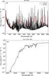 |
Fig. 1 Stellar XUV, FUV, and NUV SEDs. Panel a shows the original spectrum taken from Sanz-Forcada (in prep.), which is the same as that used in Czesla et al. (2022) and Lampón et al. (2023). The red dashed line represents the binned spectrum according to our model settings. Panel b shows the SED in FUV and NUV wavelengths, which was reconstructed based on the stellar atmosphere model of Castelli & Kurucz (2003). |
3 Results
In this section, we present the modelled He 10830 and Hα transmission spectra and compare them with the observations of Czesla et al. (2022). The wavelengths of the He 10830 triplet are 10829.09, 10830.25, and 10 830.33 Å. In our model, the two latter lines are considered as a single merged line centered at 10 830.29 Å because they are practically unresolved (Drake 1971). We use the wavelengths in air, with the wavelength range of 10828.2–10 831.8 Å considered here. The line center of Hα is at 6562.8 Å in air, and the simulations and analyses were performed in the wavelength range of [6561.0, 6564.6 Å]. In this work, we shifted the observed He 10830 and Hα data in vacuum to that in air for model comparison.
After simulating the He 10830 and Hα transmission spectra, we calculated the χ2. The data contain structures, such as the spikes in the Hα line, that cannot be reproduced by our model and are likely attributable to systematic noise. In the calculation of our χ2 value, we therefore applied the procedure suggested by Allart et al. (2023), which renormalises χ2 by dividing by the lowest obtained χ2 value. This is tantamount to enlarging the error bars, thereby accounting for systematic noise contributions. After binning the data, we have a degrees of freedom value of 52, which leads to a standard deviation of the renormalised reduced χ2 distribution of ![Mathematical equation: $\[\sigma=\sqrt{(2 \times 52)} / 52 \sim 0.2\]$](/articles/aa/full_html/2024/06/aa48210-23/aa48210-23-eq8.png) . Then we defined models with χ2 < 1.6 (within 3σ) as good-fit models of the observation.
. Then we defined models with χ2 < 1.6 (within 3σ) as good-fit models of the observation.
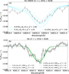 |
Fig. 2 Comparison of He 10830 and Hα transmission spectra with the models that reproduce both the lines well with solar metallicity (Z = 1) and H/He ratio (92/8). In each panel, the label in the y-axis Fin/Fout − 1 is the in-transit flux over out-of transit flux minus 1, which represents the relative absorption depth. The legends show the model parameters and the values of χ The lines with error bars are the observation data from Czesla et al. (2022). |
3.1 Modelling He 10830 and Hα transmission spectra with solar metallicity (Z = 1)
3.1.1 H/He = 92/8
Figure 2a shows the transmission spectra of He 10830 for models with solar metallicity (Z = 1) and the fiducial hydrogen-to-helium abundance ratio (H/He = 92/8). We find that the He 10830 absorption is very sensitive to the change of FXUV. A high FXUV tends to lead to a high absorption. In the explored parameter space of FXUV &ge 0.125F0 and βm, the model for FXUV = 0.125F0 and βm = 0.1 gives χ2 = 1.95, but still larger than 1.6 (the 3σ limit). We can see that the modelled absorption depth is obviously higher than the observation in a wide wavelength range. We then slightly decrease FXUV to 0.1F0 and 0.075F0. As FXUV decreases to 0.1 F0, χ2 decreases, then increases as it further decreases to 0.075F0. Therefore, the model of FXUV = 0.1F0 and βm = 0.1 gives the lowest &chi2 value in the parameter space and can explain the He 10830 observation well.
In Fig. 2b, we show models that can explain the Hα line with FXUV = 0.1 (0.125)F0 and βm = 0.1. We find that, unlike He 10830, changing the XUV flux from 0.1F0 to 0.125F0 does not result in a significant change of the Hα absorption depth, as can be seen in the dash-dotted lines in Fig. 2b. However, in this case, a stellar Lyα flux as high as 300–400 times the fiducial value is required (FLyα/![Mathematical equation: $\[F_{\mathrm{Ly} \alpha_0}\]$](/articles/aa/full_html/2024/06/aa48210-23/aa48210-23-eq9.png) ≈ 300–400). This corresponds to (1.2–1.6) × 107 erg cm−2 s−1, which is about 0.5% of the bolometric flux received from the star (~2.39 × 10⁹ erg cm−2 s−1). Linsky et al. (2013) investigated the ratio of Lyα flux to X-ray flux for stars with different stellar types, establishing an upper limit below 100 (approximately 60–80) and a lower limit of around 0.6 for F5V-G9V stars. In our work, the fiducial X-ray luminosity is about 2.3 × 1029 erg s−1, so the fiducial X-ray flux at the planetary orbit
≈ 300–400). This corresponds to (1.2–1.6) × 107 erg cm−2 s−1, which is about 0.5% of the bolometric flux received from the star (~2.39 × 10⁹ erg cm−2 s−1). Linsky et al. (2013) investigated the ratio of Lyα flux to X-ray flux for stars with different stellar types, establishing an upper limit below 100 (approximately 60–80) and a lower limit of around 0.6 for F5V-G9V stars. In our work, the fiducial X-ray luminosity is about 2.3 × 1029 erg s−1, so the fiducial X-ray flux at the planetary orbit ![Mathematical equation: $\[F_{\mathrm{X}_0}\]$](/articles/aa/full_html/2024/06/aa48210-23/aa48210-23-eq10.png) is about 6.95 × 10⁴ erg cm−2 s−1. For the model of FXUV = 0.1F0, the X-ray flux FX =
is about 6.95 × 10⁴ erg cm−2 s−1. For the model of FXUV = 0.1F0, the X-ray flux FX = ![Mathematical equation: $\[0.1 F_{\mathrm{X}_0}\]$](/articles/aa/full_html/2024/06/aa48210-23/aa48210-23-eq11.png) = 6.95 × 10³ erg cm−2 s−1. Therefore, FLyα/FX ~ (1700–2300), which is one order of magnitude higher than the upper limit in Linsky et al. (2013). Increasing the XUV flux FXUV and spectral index βm can mitigate the requirement of such a high stellar Lyα flux. For instance, the lime solid line in Fig. 2b shows that for the model with FXUV = 0.125F0, when βm increases to 0.3, we obtained a reduction of
= 6.95 × 10³ erg cm−2 s−1. Therefore, FLyα/FX ~ (1700–2300), which is one order of magnitude higher than the upper limit in Linsky et al. (2013). Increasing the XUV flux FXUV and spectral index βm can mitigate the requirement of such a high stellar Lyα flux. For instance, the lime solid line in Fig. 2b shows that for the model with FXUV = 0.125F0, when βm increases to 0.3, we obtained a reduction of ![Mathematical equation: $\[F_{\mathrm{Ly} \alpha} / F_{\mathrm{Ly} \alpha_0}\]$](/articles/aa/full_html/2024/06/aa48210-23/aa48210-23-eq12.png) ≈ 200 to fit the absorption line. However, low FXUV and βm are preferred for explaining the He 10830 observation.
≈ 200 to fit the absorption line. However, low FXUV and βm are preferred for explaining the He 10830 observation.
3.1.2 H/He = 99/1, 99.5/0.5, and 99.9/0.1
The reason very low FXUV and βm are needed for models with H/He = 92/8 to explain the He 10830 observation is that a much lower population of metastable helium is necessary in the upper atmosphere. In this section, we attempt to explain the observations by reducing the helium abundance, that is, increasing H/He to 99/1, 99.5/0.5, or 99.9/0.1.
Figure 3 shows the models for various H/He ratios that can fit both the He 10830 and Hα observations. Here, for every H/He case, we initially identified those models that can fit the He 10830 observation and subsequently selected from these models the ones that can fit the Hα observation. We note that there could be additional models that match the Hα observation, but they are not included in the plot because they do not align with the He 10830 observation. Although we present results with βm ≥ 0.4, it is noteworthy that this value of βm may be unrealistically high, since a spectral index of βm ≥ 0.4 is not commonly seen for F-type stars (Sanz-Forcada et al. 2011). Therefore, we have aimed to identify and define models with βm < 0.4 as good fits for both lines.
We found that the models with high FXUV and βm tend to lead to high absorption levels. The hydrogen-to-helium abundance ratio also affects the He 10830 absorption significantly; increasing the H/He ratio, an increase in FXUV and βm are necessary for explaining the observations. It can be seen that when H/He = 99/1, only the models with 0.25F0 ≤ FXUV ≤ 0.5F0 can match the He 10830 observation. To explain the Hα absorption, a stellar Lyα flux needs to be as high as 100 times the fiducial value. In this case, FLyα/FX ~ (115–230) is still a few times higher than the upper limit in Linsky et al. (2013). For H/He = 99.5/0.5, models with 0.5F0 ≤ FXUV ≤ 1.5F0 can match the He 10830 observation and a stellar Lyα flux about ten times the fiducial value would be enough for fitting the Hα observation. Therefore, FLyα/FX decreases to about 4–12, which is well within the range of the values given in Linsky et al. (2013). FLyα = ![Mathematical equation: $\[\10 F_{\mathrm{Ly} \alpha_0}\]$](/articles/aa/full_html/2024/06/aa48210-23/aa48210-23-eq13.png) seems very high (4 × 10⁵ erg cm−2 s−1), but it is still within a reasonable range. We note that
seems very high (4 × 10⁵ erg cm−2 s−1), but it is still within a reasonable range. We note that ![Mathematical equation: $\[F_{\mathrm{Ly} \alpha_0}\]$](/articles/aa/full_html/2024/06/aa48210-23/aa48210-23-eq14.png) is a moderate value for the F-type stars in Linsky et al. (2013). During the X-ray observations of HAT-P-32b by Sanz-Forcada et al. (in prep.) and Czesla et al. (2022), a flare was detected, emphasising the high activity of the star. Such high activity implies that the stellar Lyα flux would also be high. For example, WASP-121 was also an active star according to Huang et al. (2023) and its FLyα was inferred to be about 1 × 10⁵ erg cm−2 s−1 at the planetary orbit. Therefore, the high FLyα is justified for HAT-P-32.
is a moderate value for the F-type stars in Linsky et al. (2013). During the X-ray observations of HAT-P-32b by Sanz-Forcada et al. (in prep.) and Czesla et al. (2022), a flare was detected, emphasising the high activity of the star. Such high activity implies that the stellar Lyα flux would also be high. For example, WASP-121 was also an active star according to Huang et al. (2023) and its FLyα was inferred to be about 1 × 10⁵ erg cm−2 s−1 at the planetary orbit. Therefore, the high FLyα is justified for HAT-P-32.
However, for models with H/He = 99.9/0.1, values of FXUV ≥ 2.0F0 and βm ≥ 0.3 are needed. In particular, βm ≥ 0.4 is required in most cases; βm = 0.3 only appears for FXUV = 3.0F0. In the models with FXUV = 3.0F0 and βm = 0.3, FLyα = 5![Mathematical equation: $\[F_{\mathrm{Ly} \alpha_0}\]$](/articles/aa/full_html/2024/06/aa48210-23/aa48210-23-eq15.png) , which is almost equal to the X-ray flux, would be sufficient to fit the Hα line absorption profile within 3σ; FLyα = 10
, which is almost equal to the X-ray flux, would be sufficient to fit the Hα line absorption profile within 3σ; FLyα = 10![Mathematical equation: $\[F_{\mathrm{Ly} \alpha_0}\]$](/articles/aa/full_html/2024/06/aa48210-23/aa48210-23-eq16.png) can give a lower χ2, and thus a better fit. Such high FXUV and βm values could be possible if the host star HAT-P-32 had a high activity when the absorptions of Hα and He 10830 were observed. Therefore, from the above analyses, it is likely that the H/He ratio is higher than 99/1 in the upper atmosphere of this planet.
can give a lower χ2, and thus a better fit. Such high FXUV and βm values could be possible if the host star HAT-P-32 had a high activity when the absorptions of Hα and He 10830 were observed. Therefore, from the above analyses, it is likely that the H/He ratio is higher than 99/1 in the upper atmosphere of this planet.
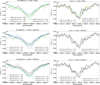 |
Fig. 3 He 10830 and Hα transmission spectra of the models with H/He = 99/1, 99.5/0.5, and 99.9/0.1 that fit the observation. The lines with error bars are the observation data from Czesla et al. (2022). |
3.2 Modelling He 10830 and Hα transmission spectra with super-solar metallicity (Z > 1)
According to Alam et al. (2020), the lower atmosphere of HAT-P-32b has a metallicity of ![Mathematical equation: $\[\log \left(Z / Z_{\odot}\right)=2.41_{-0.07}^{+0.06}\]$](/articles/aa/full_html/2024/06/aa48210-23/aa48210-23-eq17.png) (note: this Z is different to the dimensionless Z used in our work), corresponding to 218–300 times the solar metallicity. Is it possible that the upper atmosphere also exists a super-solar metallicity? To answer this question, we investigated whether the metals can rise into the upper atmosphere and eventually escape. Hunten et al. (1987) proposed that heavy species can be dragged by light ones through collisions if the mass of heavy species is smaller than the crossover mass (Xing et al. 2023). Here, we examined the oxygen species in the atmosphere of HAT-P-32b and found that the mass of oxygen is smaller than its crossover mass. This indicates that oxygen can be dragged into the upper atmosphere. Other heavy species may also escape because the crossover mass is one or two orders of magnitude higher than the mass of oxygen.
(note: this Z is different to the dimensionless Z used in our work), corresponding to 218–300 times the solar metallicity. Is it possible that the upper atmosphere also exists a super-solar metallicity? To answer this question, we investigated whether the metals can rise into the upper atmosphere and eventually escape. Hunten et al. (1987) proposed that heavy species can be dragged by light ones through collisions if the mass of heavy species is smaller than the crossover mass (Xing et al. 2023). Here, we examined the oxygen species in the atmosphere of HAT-P-32b and found that the mass of oxygen is smaller than its crossover mass. This indicates that oxygen can be dragged into the upper atmosphere. Other heavy species may also escape because the crossover mass is one or two orders of magnitude higher than the mass of oxygen.
It is important to note that we did not consider metal cooling in this work; thus, the escaping flux may be overestimated to some degree and so could be the crossover mass. However, an upper atmosphere that would simultaneously have a super-solar metallicity and a solar H/He ratio seems unlikely. In any case, as we show below, from the joint analysis of He 10830 and Hα absorptions, a super-solar upper atmosphere can be ruled out.
Increasing the metallicity in the upper atmosphere can cause significant changes to the atmospheric structures and, thus, to the He 10830 and Hα absorption profiles. Figure 4 shows the atmospheric structures for the models with H/He = 92/8, FXUV = F0, and βm = 0.16, for metallicities ranging from Z = 1 to Z = 200. Figure 5 shows the He 10830 and Hα transmission spectra of these models.
Figure 4a shows the atmospheric temperature and velocity. The temperature increases by XUV heating and decreases primarily via adiabatic expansion. The peak temperature increases with increasing metallicity. The velocity increases with altitude and become supersonic beyond the sonic points (denoted by the asterisks in the plot). At the outer boundary of the atmosphere, it exceeds about 80 km s−1. As the metallicity increases, the velocity decreases, and the sonic points tend to be at higher altitudes. Figure 4b shows the densities of H(1s) and H+. H(1s) dominates at small radii, while H+ becomes more abundant beyond r ≈ 1.1–1.3 RP. For Z < 10, an increase in metallicity would lead to higher number densities of H(1s) and H+, while the opposite holds true for Z > 10. High metallicity (Z > 10) also tends to create to an ionisation front at lower altitude, the altitude where the number densities of H(1s) and H+ are equal. Figures 4c and d show the densities of He, He+, and metastable H(23S). The number density of He(23S) has a similar profile to that of He+, indicating a close relationship between the production of He(23S) and the number density of He+. In fact, studies have shown that the recombination of He+ is the dominant process of producing He(23S) (Oklopčić 2019; Lampón et al. 2021b; Czesla et al. 2022; Yan et al. 2022). Similarly to hydrogen, the number densities of helium species decrease with the increase in metallicity for Z > 10, but the opposite occurs for Z < 10. Zhang et al. (2022b) also found that the population of metastable helium does not change monotonously with metalliciy.
As a result, the He 10830 and Hα absorptions first increase with the metallicity when Z < 10, and then decrease significantly when Z > 10 (as seen from Fig. 5). For the model with H/He = 92/8, FXUV = F0, and βm = 0.16, solar metallicity can lead to an absorption depth of He 10830 higher than 30% and it can be reduced to less than 10% when Z = 200. Introducing a higher metallicity, as suggested by the transmission spectroscopy of the lower atmosphere (Alam et al. 2020), may possibly mitigate the requirement for a high H/He ratio to fit the He 10830 absorption, as discussed.
In Fig. 6, we show the transmission spectra of He 10830 and Hα for models with Z = 100, 200, and 300, when keeping the H/He ratio as 92/8. For these models, the reduced χ2 values are all larger than 1.6 (3σ), so we showed the results with χ2 < 3. It can be seen that for Z = 100, only models with FXUV ≤ 0.25F0 can give χ2 < 3 for the He 10830 transmission spectra. The He 10830 absorption changes slightly with the spectral index βm. For these models, a stellar Lyα flux as high as 1000 times the fiducial value is required to explain the Hα observation. For Z = 200, FXUV is about (0.25–1.5) F0, and FLyα should be about ![Mathematical equation: $\[4000 F_{\text Ly \alpha_0}\]$](/articles/aa/full_html/2024/06/aa48210-23/aa48210-23-eq18.png) ; and for Z = 300, FLyα increases to 10000–20000 times the fiducial value. As shown in the Sec. 3.1, such a high FLyα is unlikely. Therefore, while a super-solar metallicity (100 times higher than the solar value) could occur in the lower atmosphere of HAT-P-32b, a nearly solar metallicity can be present in the upper atmosphere.
; and for Z = 300, FLyα increases to 10000–20000 times the fiducial value. As shown in the Sec. 3.1, such a high FLyα is unlikely. Therefore, while a super-solar metallicity (100 times higher than the solar value) could occur in the lower atmosphere of HAT-P-32b, a nearly solar metallicity can be present in the upper atmosphere.
Therefore, while a super-solar metallicity (100 times higher than the solar value) could occur in the lower atmosphere of HAT-P-32b, a nearly solar metallicity may be present in the upper atmosphere. On the one hand, it is possible that light species (hydrogen and helium), and even metals in the form of atoms, ions, or some molecules, rise into the upper atmosphere. However, the escaping metals may only constitude a small proportion of the total metals. As suggested by Alam et al. (2020), the high metallicity in their study of HAT-P-32b is probably indicative of a thick cloud deck or haze, where metals exist in the form of submicron-sized particles, such as magnesium silicate (Mallonn & Wakeford 2017), which cannot rise into the upper atmosphere. On the other hand, the escaping hydrogen and helium also contributes to a reduction in the mass fraction of metals in the upper atmosphere.
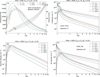 |
Fig. 4 Atmospheric structure of HAT-P-32b for models of H/He = 92/8, FXUV = F0, and βm = 0.16, but with different metallicities range from Z = 1 to Z = 200. (a) Temperature (denoted in solid lines) and velocity (dashed lines). The asterisks on the velocity lines represent the sonic points. (b) Number densities of hydrogen atoms H(1s) and ions H+. (c) Number densities of helium atoms He and ions He+. (d) Number densities of helium atoms in the metastable state, He(23S). |
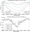 |
Fig. 5 Comparison of He 10830 and Hα transmission spectra with the models of H/He = 92/8, FXUV = F0, and βm = 0.16 for metallicities ranging from Z = 1 to Z = 200. The stellar Lyα flux is 100 times the fiducial value, i.e. FLyα = |
![Mathematical equation: $\[100 F_{\mathrm{Ly} \alpha_0}\]$](/articles/aa/full_html/2024/06/aa48210-23/aa48210-23-eq19.png)
3.3 Best-fit models
In summary, we found four best-fit models that reproduce both observations simultaneously: (1) Z = 1, H/He = 99.5/0.5, FXUV = 0.5F0, βm = 0.3, and the mass-loss rate ![Mathematical equation: $\[\dot{M}\]$](/articles/aa/full_html/2024/06/aa48210-23/aa48210-23-eq20.png) = 1.0 × 10¹³ g s−1;(2) Z = 1, H/He = 99.5/0.5, FXUV = 1.0F0, βm = 0.16, and
= 1.0 × 10¹³ g s−1;(2) Z = 1, H/He = 99.5/0.5, FXUV = 1.0F0, βm = 0.16, and ![Mathematical equation: $\[\dot{M}\]$](/articles/aa/full_html/2024/06/aa48210-23/aa48210-23-eq21.png) = 1.5 × 10¹³ g s−1; (3) Z = 1, H/He = 99.5/0.5, FXUV = 1.5F0, βm = 0.1, and
= 1.5 × 10¹³ g s−1; (3) Z = 1, H/He = 99.5/0.5, FXUV = 1.5F0, βm = 0.1, and ![Mathematical equation: $\[\dot{M}\]$](/articles/aa/full_html/2024/06/aa48210-23/aa48210-23-eq22.png) = 1.8 × 10¹³ g s−1; (4) Z = 1, H/He = 99.9/0.1, FXUV = 3.0F0, βm = 0.3, and
= 1.8 × 10¹³ g s−1; (4) Z = 1, H/He = 99.9/0.1, FXUV = 3.0F0, βm = 0.3, and ![Mathematical equation: $\[\dot{M}\]$](/articles/aa/full_html/2024/06/aa48210-23/aa48210-23-eq23.png) = 3.1 × 10¹³ g s−1. The He 10830 and Hα transmission spectra of these models are shown in Fig. 7. The resulting mass-loss rate of about, approximately (1.0 − 3.1) × 1013 g s−1, is consistent with those from the energy-limited approach applying a very low heating efficiency, and with those of Czesla et al. (2022) and Lampón et al. (2023). The H/He ratio of ≥99.5/0.5 is also consistent with that of Lampón et al. (2023), who concluded that the H/He ratio in the upper atmosphere of HAT-P-32b is
= 3.1 × 10¹³ g s−1. The He 10830 and Hα transmission spectra of these models are shown in Fig. 7. The resulting mass-loss rate of about, approximately (1.0 − 3.1) × 1013 g s−1, is consistent with those from the energy-limited approach applying a very low heating efficiency, and with those of Czesla et al. (2022) and Lampón et al. (2023). The H/He ratio of ≥99.5/0.5 is also consistent with that of Lampón et al. (2023), who concluded that the H/He ratio in the upper atmosphere of HAT-P-32b is ![Mathematical equation: $\[(99.0 / 1.0)_{-10}^{+0.5}\]$](/articles/aa/full_html/2024/06/aa48210-23/aa48210-23-eq24.png) . The H/He ratio of approximately 99.5/0.5 is significantly higher than the solar value (92/8), indicating a substantial reduction in the helium abundance in the upper atmosphere. There exists a degeneracy in the combination of the XUV flux and spectral index βm. Our fiducial model assumes FXUV = 1.0F0 and βm = 0.16, the same values as adopted in Czesla et al. (2022) and Lampón et al. (2023). Other combinations, such as FXUV = 0.5F0 and βm = 0.3, FXUV = 1.5F0 and βm = 0.1, FXUV = 3.0F0 and βm = 0.3, also give reasonable results. The XUV flux was obtained using the XMM-Newton data observed on 30 August 2019, but the Hα and He 10830 transmission data were observed on 1 September and 9 December 2018, respectively. The XUV flux might have been lower in 2018 when Hα and He 10830 lines were observed. At the same time, it is also possible that the X-ray fraction could be 30% of the XUV flux, higher than in the fiducial model, because the stellar activity can vary over time in such an active host star. It is also possible that both the XUV flux FXUV and the spectral index βm exceed the fiducial values, as indicated by the fourth best-fit model, due to a high stellar activity.
. The H/He ratio of approximately 99.5/0.5 is significantly higher than the solar value (92/8), indicating a substantial reduction in the helium abundance in the upper atmosphere. There exists a degeneracy in the combination of the XUV flux and spectral index βm. Our fiducial model assumes FXUV = 1.0F0 and βm = 0.16, the same values as adopted in Czesla et al. (2022) and Lampón et al. (2023). Other combinations, such as FXUV = 0.5F0 and βm = 0.3, FXUV = 1.5F0 and βm = 0.1, FXUV = 3.0F0 and βm = 0.3, also give reasonable results. The XUV flux was obtained using the XMM-Newton data observed on 30 August 2019, but the Hα and He 10830 transmission data were observed on 1 September and 9 December 2018, respectively. The XUV flux might have been lower in 2018 when Hα and He 10830 lines were observed. At the same time, it is also possible that the X-ray fraction could be 30% of the XUV flux, higher than in the fiducial model, because the stellar activity can vary over time in such an active host star. It is also possible that both the XUV flux FXUV and the spectral index βm exceed the fiducial values, as indicated by the fourth best-fit model, due to a high stellar activity.
3.4 The atmospheric structures of the best-fit models
In this section, we present the atmospheric structures and Lyα radiation intensity within the atmosphere for the best-fit models. Figure 8 shows the atmospheric temperature, velocity, and number densities of the hydrogen and helium species. They exhibit similar trends to those in Fig. 4. However, it is noteworthy that the temperatures for the best-fit models fall within the range of 11 400–13 200 K, consistent with the results reported by Lampón et al. (2023). Additionally, the velocity near 2.4RP is also similar to that of Czesla et al. (2022) and García Muñoz & Schneider (2019).
Using the atmospheric structures of H(1s) and H+, we performed the Lyα radiative transfer simulation, obtaining the Lyα radiation intensity within the atmosphere and the H(2) population responsible for the Hα absorption. Figure 9 shows the scattering rate Pα and H(2) number density distributions in the cylindrical coordinates of the atmosphere obtained from the best-fit model. The scattering rate ![Mathematical equation: $\[P \alpha=B_{12} \bar{J}_{\mathrm{Ly} \alpha}\left[\mathrm{s}^{-1}\right]\]$](/articles/aa/full_html/2024/06/aa48210-23/aa48210-23-eq25.png) is the number of scatterings per second experienced by a hydrogen atom, where
is the number of scatterings per second experienced by a hydrogen atom, where ![Mathematical equation: $\[\bar{J}_{\mathrm{Ly} \alpha}\]$](/articles/aa/full_html/2024/06/aa48210-23/aa48210-23-eq26.png) and B12 are the Lyα radiation intensity averaged over the solid angle and the Einstein absorption B coefficient, respectively. Higher scattering numbers per second per H atom are related to a higher Lyα intensity, thus cause larger H(2) populations. For the sake of brevity, we only show the results of one representative model with H/He = 99.5/.5, FXUV = F0, and βm = 0.16. Similar results are found for the other three best-fit models. In Fig. 9, the white disks denote the planet and the surroundings are the atmosphere. The z-axis connects the centers of the star and the planet. In panels a and c, the stellar Lyα photons are incident from the bottom. Figure 9a shows Pα calculated for the stellar Lyα, which has a cylindrical symmetry. We can see that the Pα in the dayside is much higher than that in the nightside for the stellar Lyα case. The result is similar to what we found in Paper I. The Pα value calculated for the planetary Lyα shown in Fig. 9b, however, is spherically symmetric. Comparing Figs. 9a and b, we find that in most regions (except for a small part in the shadow of the planet), Pα by the planetary Lyα is much lower than by the stellar one and is negligible. A similar trend was found in Paper I. However, this is different from the results of HD 189733b and WASP-121b reported by Huang et al. (2017, 2023). In that work, it was shown that
and B12 are the Lyα radiation intensity averaged over the solid angle and the Einstein absorption B coefficient, respectively. Higher scattering numbers per second per H atom are related to a higher Lyα intensity, thus cause larger H(2) populations. For the sake of brevity, we only show the results of one representative model with H/He = 99.5/.5, FXUV = F0, and βm = 0.16. Similar results are found for the other three best-fit models. In Fig. 9, the white disks denote the planet and the surroundings are the atmosphere. The z-axis connects the centers of the star and the planet. In panels a and c, the stellar Lyα photons are incident from the bottom. Figure 9a shows Pα calculated for the stellar Lyα, which has a cylindrical symmetry. We can see that the Pα in the dayside is much higher than that in the nightside for the stellar Lyα case. The result is similar to what we found in Paper I. The Pα value calculated for the planetary Lyα shown in Fig. 9b, however, is spherically symmetric. Comparing Figs. 9a and b, we find that in most regions (except for a small part in the shadow of the planet), Pα by the planetary Lyα is much lower than by the stellar one and is negligible. A similar trend was found in Paper I. However, this is different from the results of HD 189733b and WASP-121b reported by Huang et al. (2017, 2023). In that work, it was shown that ![Mathematical equation: $\[\bar{J}_{\mathrm{Ly} \alpha}\]$](/articles/aa/full_html/2024/06/aa48210-23/aa48210-23-eq27.png) resulting from recombination inside the planetary atmosphere can exceed that of the external stellar Lyα within a certain altitude range for HD 189733b; additionally,
resulting from recombination inside the planetary atmosphere can exceed that of the external stellar Lyα within a certain altitude range for HD 189733b; additionally, ![Mathematical equation: $\[\bar{J}_{\mathrm{Ly} \alpha}\]$](/articles/aa/full_html/2024/06/aa48210-23/aa48210-23-eq28.png) from collisional excitation can become dominant in some regions for WASP-121b. The difference between our results and theirs could be due to the differences in the planetary parameters and the atmospheric geometries (spherical in our study vs plane-parallel in theirs).
from collisional excitation can become dominant in some regions for WASP-121b. The difference between our results and theirs could be due to the differences in the planetary parameters and the atmospheric geometries (spherical in our study vs plane-parallel in theirs).
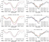 |
Fig. 6 Comparisons of the He 10830 and Hα transmission spectra with the observations, for the models with Z = 100, 200, and 300. The lines with error bars are the observation data from Czesla et al. (2022). |
4 Discussion
4.1 Effects of Lyα cooling and heating
When a Lyα photon is emitted by an atom, the atom loses energy unless the photon is reabsorbed. During the resonant scattering processes of Lyα photons, energy is conserved in the rest frame of the atom if the recoils of hydrogen atoms are negligible. Consequently, the gas cools down as it emits Lyα photons. Lyα photons created in the atmosphere have three destinations. First, they can escape the atmosphere after many resonance scatterings, which plays an important role in cooling the atmosphere. Second, they can be absorbed by dust grains and molecular hydrogen (Neufeld 1990). Third, they can be absorbed by the planetary surface, which can be regarded as cooling of the atmosphere. In our simulations, there is no dust, but there is molecular hydrogen H2 at the lower boundary of the upper atmosphere. Molecular hydrogen will be rapidly dissociated or ionised by stellar XUV radiation. However, the resonance-like absorption of Lyα by molecular hydrogen is not considered in our simulation. Therefore, the Lyα photons escape freely from the atmosphere in our simulations.
In this work, the Lyα cooling due to collisional excitation is considered in the hydrodynamic simulations. The cooling rate was calculated using ΛLyα = −7.5 × 10⁻¹⁹nen1se−118348K/T erg cm−3 s−1 (Black 1981; Murray-Clay et al. 2009), where ne and n1s are the number densities of electrons and neutral hydrogen atoms, respectively. Lyα photons can also be generated through the recombination of H+. Ignoring this process may result in some underestimation of the cooling.
However, the recoil of hydrogen atoms due to resonance scattering transfers a portion of Lyα energy to the hydrogen atoms, eventually heating the hydrogen gas. Depending on the scattering angle, an atom’s recoil can result in either energy gain or loss, but when averaged over the entire scattering angle, it ultimately leads to net heating. The heating induced by Lyα scattering has been studied in cosmology (Madau et al. 1997; Chen & Miralda-Escudé 2004). However, there is some debate regarding the significance of the heating rate. Madau et al. (1997) first pointed out the heating from Lyα scattering and demonstrated its potential criticality. In contrast, Chen & Miralda-Escudé (2004) argued that the heating induced by Lyα scattering is negligible. It is unclear how significant the heating by recoil of hydrogen atoms caused by resonance scattering would be in the planetary atmosphere. However, the heating rate will be likely to be significantly smaller than the cooling rate induced by collisional excitation and recombination. This is because the heating by recoil is an average over the scattering angle. It was also found that the imprint of the recoil effect on the Lyα spectral profile near the line center is not clearly appreciable in a high-temperature (T ~ 104 K) gas in the context of Wouthuysen–Field effect, which is closely associated with the Lyα heating (Seon & Kim 2020).
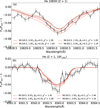 |
Fig. 7 Model transmission spectra that fit both the He 10830 and Hα observations. The lines with error bars are the observation data from Czesla et al. (2022). |
4.2 Effects of turbulence and limb darkening
In this work, the Voigt profile is used when calculating the absorption profiles of He 10830 and Hα. The hydrodynamic bulk velocity and the thermal velocity contribute to the line broadening. In addition to these broadening components, there can be turbulence in the atmosphere. The turbulence effect can be described by adopting an effective Doppler width ![Mathematical equation: $\[\Delta v_{\mathrm{D}}=\frac{v_0}{c}(\frac{2 k T}{m}+v_{\text {turb }}^2)^{1 / 2}\]$](/articles/aa/full_html/2024/06/aa48210-23/aa48210-23-eq29.png) in place of the thermal Doppler width, where υturb is the turbulence velocity (Rybicki & Lightman 1986; Seon & Kim 2020). The line broadening by turbulence has been included when calculating the transmission spectra of exoplanetary atmosphere in some works (Salz et al. 2018; Lampón et al. 2020; Czesla et al. 2022). These authors assumed that the turbulence velocity
in place of the thermal Doppler width, where υturb is the turbulence velocity (Rybicki & Lightman 1986; Seon & Kim 2020). The line broadening by turbulence has been included when calculating the transmission spectra of exoplanetary atmosphere in some works (Salz et al. 2018; Lampón et al. 2020; Czesla et al. 2022). These authors assumed that the turbulence velocity ![Mathematical equation: $\[v_{\text {turb }}=\sqrt{5 \mathrm{kT} / 3 {m}}\]$](/articles/aa/full_html/2024/06/aa48210-23/aa48210-23-eq30.png) , which corresponds to the speed of sound (cs) of a monatomic gas and, thus, to the transonic case with a Mach number of 1.
, which corresponds to the speed of sound (cs) of a monatomic gas and, thus, to the transonic case with a Mach number of 1.
To evaluate the effects of turbulence in line broadening, we added υturb in the Doppler width assuming the transonic case and compared the resulting transmission spectra with our nominal models (without turbulence). Figure 10 shows the transmission spectra of He 10830 and Hα for the models of H/He = 99.5, FXUV = 1F0, and βm = 0.16, when the turbulence velocity varies. The solid and dash-dotted lines represent the nominal models and those with turbulence, respectively. It is found that for He 10830, including the turbulence effect decreases the absorption depth slightly at the line center, but doesn’t significantly alter the absorption at the line wings. Similarly, the turbulence leads to a lower Hα absorption at the line center, but a deeper absorption at the line wings, resulting in a broader line profile. In these cases, one would expect a slightly higher FXUV and βm to fit both the absorption lines. However, the turbulence velocity might be different from ![Mathematical equation: $\[v_{\text {turb }}=\sqrt{5 k T / 3 m}\]$](/articles/aa/full_html/2024/06/aa48210-23/aa48210-23-eq31.png) (or cs) in a real case, and its effect in the line broadening will be altered accordingly. To demonstrate its effect, we examined the Hα and He 10830 transmission spectra of two cases, where υturb = 0.5 × cs and υturb = 1.5 × cs. It can be seen from Fig. 10 that a larger turbulence velocity tends to lead to a broader absorption line profile. In the diffuse interstellar medium (ISM), turbulence velocity exhibits an anti-correlation with gas temperature, and the Mach number is typically below 1 at temperatures in the range of a few thousand K or higher (e.g. Redfield & Linsky 2004). Therefore, while it remains uncertain whether the same trend observed in the diffuse ISM can be applied to the atmosphere, the turbulence effect is likely less significant than the one explored in this paper.
(or cs) in a real case, and its effect in the line broadening will be altered accordingly. To demonstrate its effect, we examined the Hα and He 10830 transmission spectra of two cases, where υturb = 0.5 × cs and υturb = 1.5 × cs. It can be seen from Fig. 10 that a larger turbulence velocity tends to lead to a broader absorption line profile. In the diffuse interstellar medium (ISM), turbulence velocity exhibits an anti-correlation with gas temperature, and the Mach number is typically below 1 at temperatures in the range of a few thousand K or higher (e.g. Redfield & Linsky 2004). Therefore, while it remains uncertain whether the same trend observed in the diffuse ISM can be applied to the atmosphere, the turbulence effect is likely less significant than the one explored in this paper.
Besides turbulence, there are other processes, such as stellar wind and planetary magnetic field, that can affect the line shape (MacLeod & Oklopčić 2022; Schreyer et al. 2023). For instance, Lampón et al. (2023) estimated the potential effects of stellar winds and found no significant effect on the derived range of temperature and mass-loss rate for HAT-P-32b. A detailed study of the stellar wind and planetary magnetic field requires a comprehensive 3D model, which we defer to a future work.
The surface brightness of the stellar disk changes with the limb angle (Czesla et al. 2015; Yan et al. 2015). We find that adopting different limb-darkening laws results in variations in the absorption line profiles. In Yan et al. (2022), we showed that a constant surface brightness or an isotropic intensity (Iν = constant) gives a lower absorption in both the Hα and He 10830 lines than the Eddington limb-darkening law. In this work, we also obtain the same result. The dashed lines in Fig. 10 show the transmission spectra of the models with a constant stellar surface brightness. The parameters derived in this work may vary slightly if a different limb-darkening law is assumed, but the main results will remain robust.
4.3 Escape of helium
In addition to the helium detection of HAT-P-32b by Czesla et al. (2022), an escaping helium atmosphere of this planet was also detected by Zhang et al. (2023b). The latter reported giant tidal tails of helium spanning a projected length over 53 times the planet’s radius. Using a nearly isothermal 3D hydro-dynamic model based on Athena ++, Zhang et al. (2023b) derived a mass-loss rate of 1.07 × 10¹² g s−1, approximately an order of magnitude lower than our result and those of Czesla et al. (2022) and Lampón et al. (2023). Zhang et al. (2023b) obtained the mass-loss rate by assuming an outflow temperature of about 5750 K and a solar H/He ratio. In their analysis of He triplet absorption, Czesla et al. (2022) and Lampón et al. (2023) derived, for a similar temperature and H/He to those of Zhang et al. (2023b) (T = 6000 K and an H/He of 90/10), a mass-loss rate slightly lower than 1012 g s−1. However, accounting for the 1.5-times-higher absorption measured by Zhang et al. (2023b), we estimated 1.5 times that mass-loss rate (1012 g s−1), in agreement with their result.
As of now, there are several exoplanets with detected escaping helium. On the one hand, models have shown that explaining many of the He 10830 absorption signals may require a higher H/He ratio (or lower helium abundance) than that of the Sun. However, there is still a lack of clear explanations for these elevated H/He ratios. One possible explanation could be that helium, being heavier than hydrogen, is less likely to escape. Therefore, at higher altitudes, the concentration of helium decreases. Using a multifluid hydrodynamic model, Xing et al. (2023) studied the helium fractionation in the atmosphere of HD 209458b. They found that helium atoms are hard to escape, compared to hydrogen and, thus, H/He ends up varying with altitude. The low helium abundance could thus be explained by the fractionation mechanism. In our work, the mass of helium is smaller than its crossover mass, which means there is a possibility that helium can be dragged by hydrogen into the upper atmosphere of HAT-P-32b. However, the metal-rich lower atmosphere indicate the portion of hydrogen and helium is reduced in comparison to that of the Sun. A high H/He ratio in this planet may indicate a lack of helium in the lower atmosphere in the current stage, or even during the planetary formation. The low helium abundance in the atmosphere implies the necessity of further studies of the helium escape.
On the other hand, we may question what kinds of exoplanets tend to exhibit excess He 10830 absorption. Oklopčić (2019) suggested that close-in exoplanets orbiting late-type stars, especially K-type stars, are more promising with respect to exhibiting He 10830 absorption signals. Nortmann et al. (2018) showed the 10830 excess absorption as a function of the XUVHe (5–504 Å) flux and stellar activity, finding that a higher XUVHe flux and a higher stellar activity contribute to the detectability of He 10830 excess absorption. Using similar comparing methods, Orell-Miquel et al. (2022) and Zhang et al. (2023a) also showed that planets with a relatively larger XUVHe flux tend to give a He 10830 excess absorption. Zhang et al. (2023b) examined the plots of absorption versus Roche-lobe filling, planets’ surface gravities, equilibrium temperatures, incident XUV flux, and their host stars’ effective temperatures in the exoplanets with detections and upper-limit constraints of He 10830. However, they found no clear trend of He 10830 absorption with these parameters. Allart et al. (2023) searched for helium atmosphere in a sample of eleven exoplanets and showed the He 10830 absorption as a function of stellar mass and XUVHe flux. They suggested that the dependence of He 10830 absorption on XUVHe flux is influenced by other parameters, such as the stellar mass.
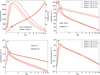 |
Fig. 8 Atmospheric structure of HAT-P-32b for the best-fit models. (a) Temperature (denoted in solid lines) and velocity (dashed lines). The asterisks on the velocity lines represent the sonic points. (b) Number densities of hydrogen atoms H(1s) and ions H+. (c) Number densities of helium atoms He and ions He+. (d) Number densities of helium atoms in the metastable state, He(23S). |
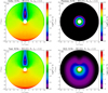 |
Fig. 9 Scattering rate, Pα, and H(2) number density distributions. (a–c) Pα obtained for the stellar, planetary Lyα, and both, respectively. (d) H(2) number density. Note: all the colorbars are given in log scale. |
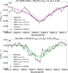 |
Fig. 10 Transmission spectra of He 10830 and Hα lines for the models with different turbulence velocities and limb-darkening laws. The solid, dash-dotted, and dashed lines represent the cases of the nominal models, the models including the turbulence effect with a velocity of 0.5 to 1.5 times the speed of sound cs, and the model with a constant stellar surface brightness (Iν = constant). The gray lines with error bars are the observation data from Czesla et al. (2022). |
5 Conclusions
In this work, we modelled the Hα and He 10830 transmission spectra of HAT-P-32b simultaneously by using a self-consistent hydrodynamic model, which is coupled with a non-local thermodynamic model to calculate the level populations of H(2) and H(23S). A Monte Carlo simulation of Lyα resonance scattering was performed to calculate the Lyα radiation intensity inside the atmosphere, which is essential to calculate the population of H(2). We fitted the Hα and He 10830 absorption lines with plausible assumptions about the stellar flux. We also provide a means to estimate the stellar Lyα flux, which is usually not directly observed. Although it is possible the heavy species can be dragged into the upper atmosphere of HAT-P-32b, using the constraints of stellar Lyα flux, we probed that the upper atmosphere of HAT-P-32b has not a super-solar metalicity, but a near solar metallicity, opposite to the lower atmosphere.
For fitting the He 10830 absorption line, relatively low FXUV and βm are needed, while to explain the Hα absorption, large FXUV, and/or βm are required. The H/He ratio does not significantly affect the Hα absorption, especially when H/He > 99/1. However, the He 10830 absorption strongly depends on H/He. In particular, for H/He = 92/8, only models with FXUV = 0.1F0 and βm = 0.1 can explain the He 10830 observation. Large FXUV > 3F0 and βm ≥ 0.3 are required for the case of H/He = 99.9/0.1. Fitting both lines simultaneously, we constrained the hydrogen-to-helium abundance ratio to be H/He ≥ 99.5/0.5, the XUV flux to be approximately (0.5–3.0) times the fiducial value (F0 = 4.2 χ 105 erg cm−2 s−1), and the spectral index βm to be about 0.16–0.3. The final models give a mass-loss rate of about (1.0–3.1)×1013g s−1 and a temperature of about 11 400–13 200 K. Our results are consistent with the previous studies (Czesla et al. 2022; Lampón et al. 2023). Moreover, our results show that the stellar Lyα flux can be as high as 4 × 10⁵ erg cm−2 s−1, consistent with the high stellar activity at the observation epoch of the Hα and He 10830 absorption.
In this paper, we investigated the transmission signals of Hα and He 10830 observed by Czesla et al. (2022) at mid-transit. In the near future, we plan to study the time series of these transmission signals in order to obtain more accurate constraints on the upper atmosphere of this planet. To study the escape of helium in more detail and find its statistical trends, more observations are needed. Advanced models both in 1D (faster and thus adequate for parameter studies) ought to be coupled with sophisticated 2D or 3D models (which include more physical processes) are needed for a detailed explanation of the observed signals, especially the asymmetric transmission features.
Acknowledgements
We thank the anonymous referees for their constructive comments, which helped improve the manuscript. This work is supported by the Strategic Priority Research Program of the Chinese Academy of Sciences, grant No. XDB 41000000, the National Key R&D Program of China (grant no. 2021YFA1600400/2021YFA1600402), the National Natural Science Foundation of China (grants nos. 11973082, 12288102 and 42305136), the Natural Science Foundation of Yunnan Province (Nos. 202201AT070158, 202401CF070041), and the International Centre of Supernovae, Yunnan Key Laboratory (no. 202302AN360001). K.-I. Seon was partly supported by a National Research Foundation of Korea (NRF) grant funded by the Korean government (MSIT; no. 2020R1A2C1005788) and by the Korea Astronomy and Space Science Institute grant funded by the Korea government (MSIT; no. 2023183000). S.C. acknowledges the support of the DFG priority program SPP 1992 “Exploring the Diversity of Extrasolar Planets” (CZ 222/5-1). The authors gratefully acknowledge the “PHOENIX Supercomputing Platform” jointly operated by the Binary Population Synthesis Group and the Stellar Astrophysics Group at Yunnan Observatories, Chinese Academy of Sciences. The IAA team acknowledges financial support from the Agencia Estatal de Investigación, MCIN/AEI/10.13039/501100011033, through grants PID2022-141216NB-I00 and CEX2021-001131-S.
References
- Alam, M. K., López-Morales, M., Nikolov, N., et al. 2020, AJ, 160, 51 [NASA ADS] [CrossRef] [Google Scholar]
- Allart, R., Bourrier, V., Lovis, C., et al. 2018, Science, 362, 1384 [Google Scholar]
- Allart, R., Lemée-Joliecoeur, P. B., Jaziri, A. Y., et al. 2023, A&A, 677, A164 [NASA ADS] [CrossRef] [EDP Sciences] [Google Scholar]
- Alonso-Floriano, F. J., Snellen, I. A. G., Czesla, S., et al. 2019, A&A, 629, A110 [NASA ADS] [CrossRef] [EDP Sciences] [Google Scholar]
- Arnaud, K. A. 1996, in Astronomical Data Analysis Software and Systems V, eds. G. H. Jacoby & J. Barnes, Astronomical Society of the Pacific Conference Series, 101, 17 [NASA ADS] [Google Scholar]
- Asplund, M., Grevesse, N., Sauval, A. J., & Scott, P. 2009, ARA&A, 47, 481 [NASA ADS] [CrossRef] [Google Scholar]
- Barnes, J. R., Haswell, C. A., Staab, D., & Anglada-Escudé, G. 2016, MNRAS, 462, 1012 [Google Scholar]
- Bello-Arufe, A., Knutson, H. A., Mendonça, J. M., et al. 2023, AJ, 166, 69 [NASA ADS] [CrossRef] [Google Scholar]
- Ben-Jaffel, L., Ballester, G. E., García Muñoz, A., et al. 2022, Nat. Astron., 6, 141 [NASA ADS] [CrossRef] [Google Scholar]
- Black, J. H. 1981, MNRAS, 197, 553 [NASA ADS] [Google Scholar]
- Borsa, F., Allart, R., Casasayas-Barris, N., et al. 2021, A&A, 645, A24 [EDP Sciences] [Google Scholar]
- Bourrier, V., Lecavelier des Etangs, A., Ehrenreich, D., et al. 2018, A&A, 620, A147 [NASA ADS] [CrossRef] [EDP Sciences] [Google Scholar]
- Cabot, S. H. C., Madhusudhan, N., Welbanks, L., Piette, A., & Gandhi, S. 2020, MNRAS, 494, 363 [Google Scholar]
- Caldiroli, A., Haardt, F., Gallo, E., et al. 2021, A&A, 655, A30 [NASA ADS] [CrossRef] [EDP Sciences] [Google Scholar]
- Casasayas-Barris, N., Pallé, E., Yan, F., et al. 2018, A&A, 616, A151 [NASA ADS] [CrossRef] [EDP Sciences] [Google Scholar]
- Castelli, F., & Kurucz, R. L. 2003, in Modelling of Stellar Atmospheres, 210, eds. N. Piskunov, W. W. Weiss, & D. F. Gray, A20 [NASA ADS] [Google Scholar]
- Cauley, P. W., Redfield, S., & Jensen, A. G. 2017, AJ, 153, 217 [NASA ADS] [CrossRef] [Google Scholar]
- Cauley, P. W., Shkolnik, E. L., Ilyin, I., et al. 2019, AJ, 157, 69 [Google Scholar]
- Cauley, P. W., Wang, J., Shkolnik, E. L., et al. 2021, AJ, 161, 152 [Google Scholar]
- Chen, X., & Miralda-Escudé, J. 2004, ApJ, 602, 1 [NASA ADS] [CrossRef] [Google Scholar]
- Chen, G., Casasayas-Barris, N., Pallé, E., et al. 2020, A&A, 635, A171 [NASA ADS] [CrossRef] [EDP Sciences] [Google Scholar]
- Christie, D., Arras, P., & Li, Z.-Y. 2013, ApJ, 772, 144 [NASA ADS] [CrossRef] [Google Scholar]
- Czesla, S., Klocová, T., Khalafinejad, S., Wolter, U., & Schmitt, J. H. M. M. 2015, A&A, 582, A51 [NASA ADS] [CrossRef] [EDP Sciences] [Google Scholar]
- Czesla, S., Lampón, M., Sanz-Forcada, J., et al. 2022, A&A, 657, A6 [NASA ADS] [CrossRef] [EDP Sciences] [Google Scholar]
- Drake, G. W. 1971, Phys. Rev. A, 3, 908 [NASA ADS] [CrossRef] [Google Scholar]
- Duvvuri, G. M., Sebastian Pineda, J., Berta-Thompson, Z. K., et al. 2021, ApJ, 913, 40 [NASA ADS] [CrossRef] [Google Scholar]
- Ehrenreich, D., Bourrier, V., Wheatley, P. J., et al. 2015, Nature, 522, 459 [Google Scholar]
- Erkaev, N. V., Kulikov, Y. N., Lammer, H., et al. 2007, A&A, 472, 329 [NASA ADS] [CrossRef] [EDP Sciences] [Google Scholar]
- Fossati, L., Guilluy, G., Shaikhislamov, I. F., et al. 2022, A&A, 658, A136 [NASA ADS] [CrossRef] [EDP Sciences] [Google Scholar]
- France, K., Loyd, R. O. P., Youngblood, A., et al. 2016, ApJ, 820, 89 [NASA ADS] [CrossRef] [Google Scholar]
- Fulton, B. J., & Petigura, E. A. 2018, AJ, 156, 264 [Google Scholar]
- García Muñoz, A., & Schneider, P. C. 2019, ApJ, 884, L43 [Google Scholar]
- Guilluy, G., Andretta, V., Borsa, F., et al. 2020, A&A, 639, A49 [EDP Sciences] [Google Scholar]
- Gully-Santiago, M., Morley, C. V., Luna, J., et al. 2023, AJ, 167, 142 [Google Scholar]
- Guo, J. H. 2011, ApJ, 733, 98 [Google Scholar]
- Guo, J. H. 2013, ApJ, 766, 102 [Google Scholar]
- Guo, J. H. 2019, ApJ, 872, 99 [NASA ADS] [CrossRef] [Google Scholar]
- Guo, J. H., & Ben-Jaffel, L. 2016, ApJ, 818, 107 [Google Scholar]
- Hartman, J. D., Bakos, G. Á., Torres, G., et al. 2011, ApJ, 742, 59 [NASA ADS] [CrossRef] [Google Scholar]
- Huang, C., Arras, P., Christie, D., & Li, Z.-Y. 2017, ApJ, 851, 150 [NASA ADS] [CrossRef] [Google Scholar]
- Huang, C., Koskinen, T., Lavvas, P., & Fossati, L. 2023, ApJ, 951, 123 [NASA ADS] [CrossRef] [Google Scholar]
- Hunten, D. M., Pepin, R. O., & Walker, J. C. G. 1987, Icarus, 69, 532 [NASA ADS] [CrossRef] [Google Scholar]
- Jensen, A. G., Redfield, S., Endl, M., et al. 2012, ApJ, 751, 86 [Google Scholar]
- Jensen, A. G., Cauley, P. W., Redfield, S., Cochran, W. D., & Endl, M. 2018, AJ, 156, 154 [Google Scholar]
- Khodachenko, M. L., Shaikhislamov, I. F., Lammer, H., et al. 2021, MNRAS, 507, 3626 [NASA ADS] [CrossRef] [Google Scholar]
- Kirk, J., Dos Santos, L. A., López-Morales, M., et al. 2022, AJ, 164, 24 [NASA ADS] [CrossRef] [Google Scholar]
- Koskinen, T. T., Lavvas, P., Huang, C., et al. 2022, ApJ, 929, 52 [NASA ADS] [CrossRef] [Google Scholar]
- Kulow, J. R., France, K., Linsky, J., & Loyd, R. O. P. 2014, ApJ, 786, 132 [Google Scholar]
- Lammer, H., Selsis, F., Ribas, I., et al. 2003, ApJ, 598, L121 [Google Scholar]
- Lampón, M., López-Puertas, M., Lara, L. M., et al. 2020, A&A, 636, A13 [NASA ADS] [CrossRef] [EDP Sciences] [Google Scholar]
- Lampón, M., López-Puertas, M., Czesla, S., et al. 2021a, A&A, 648, L7 [CrossRef] [EDP Sciences] [Google Scholar]
- Lampón, M., López-Puertas, M., Sanz-Forcada, J., et al. 2021b, A&A, 647, A129 [EDP Sciences] [Google Scholar]
- Lampón, M., López-Puertas, M., Sanz-Forcada, J., et al. 2023, A&A, 673, A140 [NASA ADS] [CrossRef] [EDP Sciences] [Google Scholar]
- Lecavelier Des Etangs, A., Ehrenreich, D., Vidal-Madjar, A., et al. 2010, A&A, 514, A72 [NASA ADS] [CrossRef] [EDP Sciences] [Google Scholar]
- Lecavelier des Etangs, A., Bourrier, V., Wheatley, P. J., et al. 2012, A&A, 543, L4 [NASA ADS] [CrossRef] [EDP Sciences] [Google Scholar]
- Linsky, J. L., France, K., & Ayres, T. 2013, ApJ, 766, 69 [Google Scholar]
- Linsky, J. L., Fontenla, J., & France, K. 2014, ApJ, 780, 61 [Google Scholar]
- Linssen, D. C., Oklopčić, A., & MacLeod, M. 2022, A&A, 667, A54 [NASA ADS] [CrossRef] [EDP Sciences] [Google Scholar]
- MacLeod, M., & Oklopčić, A. 2022, ApJ, 926, 226 [NASA ADS] [CrossRef] [Google Scholar]
- Madau, P., Meiksin, A., & Rees, M. J. 1997, ApJ, 475, 429 [NASA ADS] [CrossRef] [Google Scholar]
- Mallonn, M., & Wakeford, H. R. 2017, Astron. Nachr., 338, 773 [NASA ADS] [CrossRef] [Google Scholar]
- Murray-Clay, R. A., Chiang, E. I., & Murray, N. 2009, ApJ, 693, 23 [Google Scholar]
- Neufeld, D. A. 1990, ApJ, 350, 216 [NASA ADS] [CrossRef] [Google Scholar]
- Nortmann, L., Pallé, E., Salz, M., et al. 2018, Science, 362, 1388 [Google Scholar]
- Oklopčić, A. 2019, ApJ, 881, 133 [Google Scholar]
- Oklopčić, A., & Hirata, C. M. 2018, ApJ, 855, L11 [Google Scholar]
- Orell-Miquel, J., Murgas, F., Pallé, E., et al. 2022, A&A, 659, A55 [NASA ADS] [CrossRef] [EDP Sciences] [Google Scholar]
- Owen, J. E., & Lai, D. 2018, MNRAS, 479, 5012 [Google Scholar]
- Redfield, S., & Linsky, J. L. 2004, ApJ, 613, 1004 [NASA ADS] [CrossRef] [Google Scholar]
- Rumenskikh, M. S., Shaikhislamov, I. F., Khodachenko, M. L., et al. 2022, ApJ, 927, 238 [NASA ADS] [CrossRef] [Google Scholar]
- Rybicki, G. B., & Lightman, A. P. 1986, Radiative Processes in Astrophysics (Wiley-VCH) [Google Scholar]
- Salz, M., Czesla, S., Schneider, P. C., & Schmitt, J. H. M. M. 2016, A&A, 586, A75 [NASA ADS] [CrossRef] [EDP Sciences] [Google Scholar]
- Salz, M., Czesla, S., Schneider, P. C., et al. 2018, A&A, 620, A97 [NASA ADS] [CrossRef] [EDP Sciences] [Google Scholar]
- Sanz-Forcada, J., Micela, G., Ribas, I., et al. 2011, A&A, 532, A6 [NASA ADS] [CrossRef] [EDP Sciences] [Google Scholar]
- Schreyer, E., Owen, J. E., Loyd, R. O. P., & Murray-Clay, R. 2023, arXiv e-prints [arXiv:2310.18486] [Google Scholar]
- Seager, S., & Sasselov, D. D. 2000, ApJ, 537, 916 [Google Scholar]
- Seon, K.-i., & Kim, C.-G. 2020, ApJS, 250, 9 [NASA ADS] [CrossRef] [Google Scholar]
- Seon, K.-i., Song, H., & Chang, S.-J. 2022, ApJS, 259, 3 [NASA ADS] [CrossRef] [Google Scholar]
- Shaikhislamov, I. F., Khodachenko, M. L., Lammer, H., et al. 2021, MNRAS, 500, 1404 [Google Scholar]
- Smith, R. K., Brickhouse, N. S., Liedahl, D. A., & Raymond, J. C. 2001, ApJ, 556, L91 [Google Scholar]
- Spake, J. J., Sing, D. K., Evans, T. M., et al. 2018, Nature, 557, 68 [Google Scholar]
- Vidal-Madjar, A., Lecavelier des Etangs, A., Désert, J. M., et al. 2003, Nature, 422, 143 [Google Scholar]
- Vissapragada, S., Knutson, H. A., Jovanovic, N., et al. 2020, AJ, 159, 278 [Google Scholar]
- Vissapragada, S., Knutson, H. A., Greklek-McKeon, M., et al. 2022, AJ, 164, 234 [NASA ADS] [CrossRef] [Google Scholar]
- Xing, L., Yan, D., & Guo, J. 2023, ApJ, 953, 166 [NASA ADS] [CrossRef] [Google Scholar]
- Yan, F., & Henning, T. 2018, Nat. Astron., 2, 714 [Google Scholar]
- Yan, F., Fosbury, R. A. E., Petr-Gotzens, M. G., Zhao, G., & Pallé, E. 2015, A&A, 574, A94 [NASA ADS] [CrossRef] [EDP Sciences] [Google Scholar]
- Yan, D., Guo, J., Huang, C., & Xing, L. 2021a, ApJ, 907, L47 [NASA ADS] [CrossRef] [Google Scholar]
- Yan, F., Wyttenbach, A., Casasayas-Barris, N., et al. 2021b, A&A, 645, A22 [EDP Sciences] [Google Scholar]
- Yan, D., Seon, K.-i., Guo, J., Chen, G., & Li, L. 2022, ApJ, 936, 177 [NASA ADS] [CrossRef] [Google Scholar]
- Yang, M., & Guo, J.-h. 2018, Chinese Astron. Astrophys., 42, 81 [CrossRef] [Google Scholar]
- Yang, D., & Guo, J. 2019, ApJ, 880, 90 [CrossRef] [Google Scholar]
- Yee, S. W., Winn, J. N., Knutson, H. A., et al. 2020, ApJ, 888, L5 [Google Scholar]
- Youngblood, A., France, K., Loyd, R. O. P., et al. 2016, ApJ, 824, 101 [Google Scholar]
- Zhang, M., Cauley, P. W., Knutson, H. A., et al. 2022a, AJ, 164, 237 [NASA ADS] [CrossRef] [Google Scholar]
- Zhang, M., Knutson, H. A., Wang, L., Dai, F., & Barragán, O. 2022b, AJ, 163, 67 [NASA ADS] [CrossRef] [Google Scholar]
- Zhang, M., Knutson, H. A., Wang, L., et al. 2022c, AJ, 163, 68 [NASA ADS] [CrossRef] [Google Scholar]
- Zhang, M., Knutson, H. A., Dai, F., et al. 2023a, AJ, 165, 62 [NASA ADS] [CrossRef] [Google Scholar]
- Zhang, Z., Morley, C. V., Gully-Santiago, M., et al. 2023b, Sci. Adv., 9, eadf8736 [NASA ADS] [CrossRef] [Google Scholar]
All Tables
All Figures
|
Fig. 1 Stellar XUV, FUV, and NUV SEDs. Panel a shows the original spectrum taken from Sanz-Forcada (in prep.), which is the same as that used in Czesla et al. (2022) and Lampón et al. (2023). The red dashed line represents the binned spectrum according to our model settings. Panel b shows the SED in FUV and NUV wavelengths, which was reconstructed based on the stellar atmosphere model of Castelli & Kurucz (2003). |
| In the text | |
|
Fig. 2 Comparison of He 10830 and Hα transmission spectra with the models that reproduce both the lines well with solar metallicity (Z = 1) and H/He ratio (92/8). In each panel, the label in the y-axis Fin/Fout − 1 is the in-transit flux over out-of transit flux minus 1, which represents the relative absorption depth. The legends show the model parameters and the values of χ The lines with error bars are the observation data from Czesla et al. (2022). |
| In the text | |
|
Fig. 3 He 10830 and Hα transmission spectra of the models with H/He = 99/1, 99.5/0.5, and 99.9/0.1 that fit the observation. The lines with error bars are the observation data from Czesla et al. (2022). |
| In the text | |
|
Fig. 4 Atmospheric structure of HAT-P-32b for models of H/He = 92/8, FXUV = F0, and βm = 0.16, but with different metallicities range from Z = 1 to Z = 200. (a) Temperature (denoted in solid lines) and velocity (dashed lines). The asterisks on the velocity lines represent the sonic points. (b) Number densities of hydrogen atoms H(1s) and ions H+. (c) Number densities of helium atoms He and ions He+. (d) Number densities of helium atoms in the metastable state, He(23S). |
| In the text | |
|
Fig. 5 Comparison of He 10830 and Hα transmission spectra with the models of H/He = 92/8, FXUV = F0, and βm = 0.16 for metallicities ranging from Z = 1 to Z = 200. The stellar Lyα flux is 100 times the fiducial value, i.e. FLyα = |
| In the text | |
|
Fig. 6 Comparisons of the He 10830 and Hα transmission spectra with the observations, for the models with Z = 100, 200, and 300. The lines with error bars are the observation data from Czesla et al. (2022). |
| In the text | |
|
Fig. 7 Model transmission spectra that fit both the He 10830 and Hα observations. The lines with error bars are the observation data from Czesla et al. (2022). |
| In the text | |
|
Fig. 8 Atmospheric structure of HAT-P-32b for the best-fit models. (a) Temperature (denoted in solid lines) and velocity (dashed lines). The asterisks on the velocity lines represent the sonic points. (b) Number densities of hydrogen atoms H(1s) and ions H+. (c) Number densities of helium atoms He and ions He+. (d) Number densities of helium atoms in the metastable state, He(23S). |
| In the text | |
|
Fig. 9 Scattering rate, Pα, and H(2) number density distributions. (a–c) Pα obtained for the stellar, planetary Lyα, and both, respectively. (d) H(2) number density. Note: all the colorbars are given in log scale. |
| In the text | |
|
Fig. 10 Transmission spectra of He 10830 and Hα lines for the models with different turbulence velocities and limb-darkening laws. The solid, dash-dotted, and dashed lines represent the cases of the nominal models, the models including the turbulence effect with a velocity of 0.5 to 1.5 times the speed of sound cs, and the model with a constant stellar surface brightness (Iν = constant). The gray lines with error bars are the observation data from Czesla et al. (2022). |
| In the text | |
Current usage metrics show cumulative count of Article Views (full-text article views including HTML views, PDF and ePub downloads, according to the available data) and Abstracts Views on Vision4Press platform.
Data correspond to usage on the plateform after 2015. The current usage metrics is available 48-96 hours after online publication and is updated daily on week days.
Initial download of the metrics may take a while.