| Issue |
A&A
Volume 653, September 2021
|
|
|---|---|---|
| Article Number | A136 | |
| Number of page(s) | 22 | |
| Section | Cosmology (including clusters of galaxies) | |
| DOI | https://doi.org/10.1051/0004-6361/202141226 | |
| Published online | 24 September 2021 | |
The MUSE-Wide survey: Three-dimensional clustering analysis of Lyman-α emitters at 3.3 < z < 6
1
Leibniz-Institut für Astrophysik Potsdam (AIP), An der Sternwarte 16, 14482 Potsdam, Germany
e-mail: This email address is being protected from spambots. You need JavaScript enabled to view it.
2
Universidad Nacional Autónoma de México, Instituto de Astronomía (IA-UNAM-E), AP 106, Ensenada, 22860 BC, Mexico
3
Observatoire de Genève, Université de Genève, 51 Ch. des Maillettes, 1290 Versoix, Switzerland
4
Institute of Astronomy, University of Cambridge, Madingley Road, Cambridge CB3 0HA, UK
5
European Southern Observatory, Av. Alonso de Córdova 3107, 763 0355 Vitacura, Santiago, Chile
6
Leiden Observatory, Leiden University, PO Box 9513, 2300 RA Leiden, The Netherlands
7
Department of Physics, ETH Zurich, Wolfgang-Pauli-Strasse 27, 8093 Zurich, Switzerland
8
Kapteyn Astronomical Institute, University of Groningen, Landleven 12, 9747 AD Groningen, The Netherlands
9
Univ. Lyon, Univ. Lyon1, ENS de Lyon, CNRS, Centre de Recherche Astrophysique de Lyon UMR 5574, 69230 Saint-Genis-Laval, France
Received:
30
April
2021
Accepted:
6
July
2021
Abstract
We present an analysis of the spatial clustering of 695 Lyα-emitting galaxies (LAEs) in the MUSE-Wide survey. All objects have spectroscopically confirmed redshifts in the range 3.3 < z < 6. We employed the K-estimator, an alternative clustering statistic, adapted and optimized for our sample. We also explore the standard two-point correlation function approach, which is however less suited for a pencil-beam survey such as ours. The results from both approaches are consistent. We parametrize the clustering properties in two ways, (i) following the standard approach of modelling the clustering signal with a power law (PL), and (ii) adopting a halo occupation distribution (HOD) model of the two-halo term. Using the K-estimator and applying HOD modelling, we infer a large-scale bias of bHOD = 2.80−0.38+0.38 at a median redshift of the number of galaxy pairs ⟨zpair⟩ ≃ 3.82, while the best-fit power-law analysis gives bPL = 3.03−0.52+1.51 (r0 = 3.60−0.90+3.10 comoving h−1 Mpc and γ = 1.30−0.45+0.36). The implied typical dark matter halo (DMH) mass is log(MDMH/[h−1 M⊙]) = 11.34−0.27+0.23 (adopting b = bHOD and assuming σ8 = 0.8). We study possible dependencies of the clustering signal on object properties by bisecting the sample into disjoint subsets, considering Lyα luminosity, UV absolute magnitude, Lyα equivalent width, and redshift as variables. We find no evidence for a strong dependence on the latter three variables but detect a suggestive trend of more luminous Lyα emitters clustering more strongly (thus residing in more massive DMHs) than their lower Lyα luminosity counterparts. We also compare our results to mock LAE catalogs based on a semi-analytic model of galaxy formation and find a stronger clustering signal than in our observed sample, driven by spikes in the simulated z-distributions. By adopting a galaxy-conserving model we estimate that the Lyα-bright galaxies in the MUSE-Wide survey will typically evolve into galaxies hosted by halos of log(MDMH/[h−1 M⊙]) ≈ 13.5 at redshift zero, suggesting that we observe the ancestors of present-day galaxy groups.
Key words: large-scale structure of Universe / galaxies: high-redshift / galaxies: evolution / cosmology: observations
On sabbatical leave from IA-UNAM-E at AIP.
© ESO 2021
1. Introduction
The distribution of galaxies in the Universe forms a well defined network known as the cosmic web. This structure was formed when gravitational instabilities produced by primordial density fluctuations grew until they reached a critical density. Their collapse formed gravitationally bound dark matter halos (DMHs). These halos grow hierarchically through accretion and mergers with other halos. Their gravitational interaction with baryonic matter caused gas to fall into the growing potential wells, making the gas cool by radiation and collapse to form stars and galaxies.
The evolution of the baryonic matter distribution follows the underlying dark matter (DM) but, especially in the early stages of galaxy formation, the details of this relation and how it evolved over time are still unclear. Galaxy clustering analyses aim to constrain the masses of the typical DMHs by which these galaxies are hosted and are therefore a crucial element towards understanding the formation and evolution of galaxies (Coil 2012).
A common way to quantify galaxy clustering is through correlation functions (e.g. Gawiser et al. 2007; Zehavi et al. 2011; Ouchi et al. 2017), which express the probability of finding a tuple (usually a pair) of galaxies at a certain separation (e.g. Peebles 1980). The clustering strength (large-scale bias) and the typical DMH masses can be inferred from measured correlation functions in various ways. A widespread traditional approach is to approximate the two-point correlation function (2pcf) as a power law (Davis & Peebles 1983), while more recent methods such as halo occupation distribution (HOD) modelling (e.g. Zheng & Weinberg 2007) distinguish between the different contribution of the correlation function. In these models, pairs of galaxies either belong to the same DMH or to different DMHs.
These procedures have often been applied to galaxy surveys. At low redshifts, the major surveys cover large areas of the sky, in particular SDSS (e.g. Strauss et al. 2002; Ahumada et al. 2020) along with its successors, 2MASS (Skrutskie et al. 2006), or the 2dF Galaxy Redshift survey (Colless et al. 2012). These samples at similar luminosities revealed a modest evolution of the clustering strength between z = 1 and z = 0 together with significant clustering dependencies on various galaxy properties, such as luminosity, color, morphology, galaxy type, etc. (e.g. Norberg et al. 2002; Zehavi et al. 2002, 2011; Li et al. 2006).
At high redshifts (z > 2), galaxy samples are more limited, however. Gathering a statistically relevant number of objects and covering representative volumes of the sky is a difficult task. Photometric selection techniques are often preferred because spectroscopic observations of many faint objects are observationally too expensive. The two most common techniques involve exploiting the drop in the continuum bluewards of 912 Å (Steidel & Hamilton 1992) to search for Lyman-break galaxies (LBGs) and the use of narrow-band (NB) filters to target, for instance, the Lyα emission line of young, star-forming galaxies (Lyα emitters, LAEs).
While each selection method provides us with its own somewhat biased view of the distribution of galaxies, LAEs are particularly interesting with regard to probing the lower range of stellar masses (108 − 109 M⊙), highlighting a subset of galaxies of copiously forming stars (star formation rates of 1 − 10 M⊙ yr−1). By combining the clustering analysis of LAEs with cosmological simulations, we can connect LAEs to their descendants in the local Universe.
Statistically substantial LAE samples (> 102 objects) based on narrow-band surveys were presented by Cowie & Hu (1998), Rhoads et al. (2000), Ouchi et al. (2003, 2017), Gawiser et al. (2007), Sobral et al. (2017) and others. Generally, the NB selection method only provides LAE candidates implying that samples are contaminated by interlopers, which can be a problem for clustering studies. Obviously, since all objects selected by a given NB filter are assumed to be at the same redshift, their clustering can only be explored through the analysis of transverse angular correlations (Ouchi et al. 2003, 2010, 2017; Gawiser et al. 2007; Khostovan et al. 2019). In order to study the full three-dimensional (3D) spatial clustering behaviour of galaxies and its evolution over cosmic time, large-scale spectroscopic surveys of high-redshift galaxies with individually measured redshifts are required (Le Fèvre et al. 2005, 2015; Lilly et al. 2007; Newman et al. 2013; Guzzo et al. 2014). It has been found that the clustering strength of high-redshift galaxies is significantly higher at similar luminosities than at intermediate and low redshifts (Durkalec et al. 2014), possibly also depending on luminosity and stellar mass (e.g. Ouchi et al. 2003, 2017; Durkalec et al. 2018).
Ideally, it would be optimal to perform spectroscopy of all existing objects over a large area of the sky, with a wide redshift coverage. While such surveys are still beyond our current means, panoramic integral field units (IFUs) are currently opening up an avenue for exploring this approach, at least over modest areas. In particular, the Multi Unit Spectroscopic Explorer (MUSE, Bacon et al. 2010) on the ESO-VLT has already produced significant samples of high-redshift galaxies with unprecedented source densities of several tens or even hundreds of objects per arcmin2 (Inami et al. 2017; Urrutia et al. 2019). In this paper we explore the potential of using ≈700 LAEs selected from the MUSE-Wide survey (Herenz et al. 2017; Urrutia et al. 2019) for clustering studies. Our sample differs from previous studies of LAE clustering based on narrow-band imaging, but also from generic spectroscopic surveys requiring the preselection of targets from broad-band photometry.
In a pilot study, Diener et al. (2017) used 238 LAEs from the first 24 MUSE-Wide fields to demonstrate that MUSE-selected LAEs do indeed reveal a significant clustering signal, even though the uncertainties were still large. Here, we extend this work with a larger (threefold) sample and a refined set of analysis methods and tools. The paper is structured as follows. First, we briefly describe the data used for this work and characterize the sample. In Sect. 3, we explain our methods for measuring and analysing the clustering properties of our LAE sample. In Sect. 4, we present the results of our measurements, including a study of clustering dependencies with different galaxy parameters. In Sect. 5, we discuss our results and compare our findings to predictions from a semi-analytic galaxy formation model. In Sect. 6, we present our conclusions. The appendix of the paper is mainly dedicated to a discussion of the LAE clustering results, using the traditional two-point correlation function.
Throughout the paper, all distances are measured in comoving coordinates and given in units of h−1 Mpc, where h = H0/100 = 0.70 km s−1 Mpc−1. We use a ΛCDM cosmology and adopt ΩM = 0.3, ΩΛ = 0.7, σ8 = 0.8 and H0 = 70 km s−1 Mpc−1 (Hinshaw et al. 2013). All uncertainties represent a 1σ (68.3%) confidence interval unless otherwise stated.
2. Data
2.1. The MUSE-Wide Survey
MUSE-Wide is an untargeted 3D spectroscopic survey (Herenz et al. 2017; Urrutia et al. 2019) executed by the MUSE consortium as one of the Guaranteed Time Observations (GTO) programs. The survey covers parts of the CANDELS/GOODS-S and CANDELS/COSMOS fields and also includes eight MUSE pointings in the so-called HUDF09 parallel fields (see Urrutia et al. 2019 for details). The spectroscopic data provided by MUSE complement the rich multiwavelength data available in these fields, from which physical properties such as star formation rates or stellar masses can be derived. The full survey comprises 100 MUSE fields of 1 arcmin2 each (although there is some overlap between adjacent fields), with a depth of 1 h exposure time, each split into 4 × 900 s with 90 deg rotation between the exposures. Most fields were observed in dark time, with a seeing better than 1.0″. The spectra cover the range of 4750−9350 Å, implying a Lyα redshift range of 2.9 ≲ z ≲ 6.7.
The data reduction process we used is detailed in Urrutia et al. (2019). Emission line sources were detected and their line fluxes were measured with the Line Source Detection and Cataloguing (LSDCat, Herenz & Wisotzki 2017) software. LSDCat cross-correlates a reduced and flux-calibrated data cube with a 3D source template to find emission line sources above a given significance threshold. The resulting emission line flux limit of the survey is typically around ∼10−17 erg s−1 cm−2 for LAEs, but with considerable spread between fields and also depending on the spatial extent of the Lyα emission (Herenz et al. 2019).
After the automatic detection of emission lines, a source catalog for each field was produced through visual inspection using the QtClassify tool (Kerutt 2017). After an initial redshift guess of each object from LSDCat, refined redshifts of the LAEs were measured by fitting an asymmetric Gaussian profile to the Lyα emission line. Lyα fluxes were measured using the LSDCat measure functionality, adopting a 3D aperture of three Kron-like radii (Kron 1980); together with the redshifts, this also provides the Lyα luminosities.
Since our sample is based on emission lines without prior broadband selection, it includes galaxies with very faint continua but high equivalent widths – which can sometimes go undetected in deep Hubble Space Telescope (HST) data (Maseda et al. 2018). We identified the UV counterparts for our sample and measure their continuum flux densities and absolute UV magnitudes in various HST bands, as described in detail by Kerutt et al. (in prep.). Our Lyα equivalent widths are based on combining the Lyα fluxes measured by LSDCat and continuum flux measurements from the HST counterparts. In cases where no continuum counterpart was detected, an upper limit to the continuum flux density was used to calculate lower limits to the absolute magnitudes and equivalent widths.
2.2. LAE sample
In this paper, we focus on 68 fields of the MUSE-Wide survey located in the CANDELS/GOODS-S region, along with the HUDF09 parallel fields. Some of these fields are not yet included in the currently publicly available MUSE-Wide data; these will be part of the planned final data release. We chose to not take into account the nine central fields in the MUSE-Deep area because of their different depth and selection function, in line with our aim to approach (as much as possible) a homogeneous sample and minimize systematic effects. Furthermore, we also discard the 23 MUSE-Wide fields in the COSMOS region from this analysis because of their on average somewhat lower data quality. We kept the eight MUSE-Wide pointings in the HUDF09 fields (see Fig. 1) since they give additional power to constrain the clustering signal at larger separations. In Appendix A, we demonstrate that including the UDF09 parallels fields has no significant impact on our clustering results despite a minor decrease in the uncertainties.
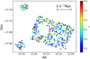 |
Fig. 1. Spatial distribution of 695 LAEs covering part of the CANDELS/GOODS-S region and the HUDF parallel fields on the left. The individual LAEs span a total of 68 fields from the MUSE-Wide survey and are color-coded by their Lyα spectroscopic redshift, 3.3 < z < 6. The 5 h−1 Mpc bar for the mean redshift of the sample |

While MUSE is formally capable of detecting LAES with 2.91 < z < 6.65, we limit the redshift range for this investigation to 3.3 < z < 6, as the details of the selection function at redshifts close to the limits are still a matter of investigation. Thus, we arrive at a final number of 695 LAEs, distributed over 62.53 arcmin2 (accounting for small field-to-field overlaps), implying an LAE density of slightly more than 11 objects per arcmin2. The sample has a mean redshift of  ≈ 4.23, the median redshift is 4.12. The transverse extent of the footprint at
  is ∼20 h−1 Mpc.
The spatial distribution of our LAEs is shown in Fig. 1, and the distribution over redshifts is presented in Fig. 2. For the latter, we replaced the usual histogram counts-per-bin by a quasi-continuous kernel density estimator (KDE) to better represent the underlying probability distribution and avoid binning artefacts. Superimposed on the KDE-filtered z distribution, we also show the distribution expected for an unclustered population of objects following the Lyα luminosity function (LF) of Herenz et al. (2019) and also factoring in the selection function of the MUSE-Wide survey. The curve has been normalized to the footprint size of our 68 fields.
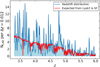 |
Fig. 2. KDE-filtered redshift distribution of the 695 LAEs of our sample, taken from 68 fields of the MUSE-Wide survey. The sample spans a redshift range of 3.3 < z < 6. The kernel is chosen to be a Gaussian with standard deviation σz = 0.005. The expected z-distribution of an unclustered population following the Lyα luminosity function of Herenz et al. (2019) and the selection function of the MUSE-Wide survey is overplotted in red. |
While the formal average accuracy of our redshifts is Δz ≃ 0.0007 or ±41 km s−1 (limited by the accuracy of fitting the line), it is well-known that Lyα peak redshifts are typically offset by up to several hundreds of km s−1 from systemic ones (e.g. Hashimoto et al. 2015; Muzahid et al. 2020; Schmidt et al. 2021), which would introduce a systematic error in the redshift-derived 3D positions of the LAEs along the line-of-sight (LOS) of the order of ∼3 Mpc. We mitigate this systematic uncertainty by applying a correction to the Lyα redshifts following the two recipes described in Verhamme et al. (2018): When the Lyα line presents two peaks with the red peak larger than the blue peak, we apply Eq. (1) from Verhamme et al. (2018). When only a single peak is visible, we employ the correction given by Eq. (2) in Verhamme et al. (2018). We show in Appendix B that our method of measuring the clustering properties is not sensitive to the details of this correction.
The range of Lyα luminosities (LLyα) of our galaxies is 40.91 < log(LLyα/[erg s−1]) < 43.33, with a median Lyα luminosity of ⟨log(LLyα/[erg s−1])⟩ = 42.36, the range of UV absolute magnitudes is −22.4 < MUV < −16.8, with a median of ⟨MUV⟩= − 18.4, and the range of rest frame equivalent widths is 10.2 < EWLyα < 794.9 Å, with a median of ⟨EWLyα⟩ = 118.3 Å.
2.3. LAE subsets
In order to explore the dependence of the clustering amplitude on physical properties of LAEs, we divide the original sample into subsamples based on different available properties. In each case we split the full sample at the median value of the LAE property under question to have (nearly) the same number of objects in each of the two subsets. The subsamples are summarized in Table 1 and defined in greater detail in the following.
Properties of the LAE samples.
A first split in redshift around ⟨z⟩ = 4.12 leads to a low-z subset of 348 LAEs with median redshift ⟨zlow⟩ = 3.56 and a high-z subset of 347 LAEs with ⟨zhigh⟩ = 4.59, respectively. The median Lyα luminosities and equivalent widths of the two redshift subsamples are nearly the same (differences of 0.08 dex and 2 Å, respectively). There is no difference between the median MUV.
In order to explore possible clustering dependencies on Lyα luminosity, we generate two subsamples divided by Lyα luminosities. We split the full sample at ⟨log(LLyα/[erg s−1])⟩ = 42.36. The low- and high-LLyα subsamples hold 349 and 346 LAEs, respectively. Their median redshifts are ⟨zlow L⟩ = 4.03 and ⟨zhigh L⟩ = 4.30. The median log(LLyα) of the subsamples differs by 0.43 dex.
While at z ≃ 3 most of our LAEs have a photometric HST counterpart, at z > 5 only around 50% of the objects are detectable in the available HST images (Kerutt et al., in prep.). Hence, for those objects we can only adopt MUV and EWLyα lower limits, which would skew the EWLyα and MUV distributions for the higher redshift subset. Therefore we decided to eliminate the LAEs without HST counterparts when splitting by EWLyα or MUV. This reduces our sample size from 695 to 509 LAEs.
We then split the HST-detected sample by equivalent width at ⟨EWLyα⟩ = 87.9 Å. The low- and high-EWLyα subsample consists of 254 and 255 LAEs, respectively. The median redshifts and luminosities of these samples are very similar (see Table 1).
Finally, we divided the HST-detected LAE sample by absolute magnitude at ⟨MUV⟩= − 18.8, leading to low- and high-MUV subsets (bright and faint, respectively) of 256 and 253 LAEs. The ⟨MUV⟩ values differ between these two subsamples by 1.59 dex, while the ⟨log(LLyα)⟩ values differ by only 0.32 dex.
3. Methods
3.1. K-estimator
3.1.1. Basic principles
The specifics of MUSE as a survey instrument present a serious challenge for the commonly used two-point correlation function (2pcf) to measure galaxy clustering. By design, MUSE surveys span a wide redshift range but cover only small (spatial) regions in the sky. The MUSE-Wide footprint has already the largest transverse footprint of all MUSE surveys, but its nature is still that of a pencil-beam survey. While transverse scales in the MUSE-Wide survey span up to ∼20 h−1 Mpc, radial scales exceed the 1000 h−1 Mpc. The limitations of the transverse extent impede the application of the ‘jackknife’ technique to compute realistic uncertainties (see Sect. 3.1.3), while methods such as bootstrapping fail in the 2pcf. Besides, given our spatial ranges, exploiting the redshift coverage rather than the spatial extent is strongly preferred. We thus explore possible alternatives to the 2pcf. In Diener et al. (2017) we applied the so-called K-estimator, introduced by Adelberger et al. (2005) to analyse the clustering of Lyman Break Galaxies, in a subset of our pencil-beam survey. Here, we build on our previous work by extending it to a larger dataset, but also paying attention to optimization aspects and comparing the method with the 2pcf.
The K-estimator focuses on radial clustering along the line of sight (LOS) by counting pair separations in redshift space at fixed transverse distances. In contrast to the 2pcf, no random sample is needed because the K-estimator computes the ratio between small and small+large scales. This quantity is directly related to the underlying correlation function. We adopt the following notation: Considering two galaxies with indices i and j, their transverse distance is Rij (equivalent to rp in the 2pcf), and their LOS redshift-space separation is Zij (equivalent to π in the 2pcf). We then count the number N of pairs within a given Rij bin, for two different ranges of Zij, |a1|< Zij < |a2| and |a2|< Zij < |a3|. The K-estimator is defined as the ratio of the numbers of galaxy pairs Na1, a2(Rij) and Na2, a3(Rij) between these two consecutive cylindrical shells, namely:
 (1)
(1)
as a function of transverse separation Rij. We set a1 = 0 h−1 Mpc so that the K-estimator quantifies the excess of galaxy pairs in the range 0 < Zij < a2 with respect to the larger LOS range of 0 < Zij < a3. In other words, the K-estimator can be expressed as K(Rij) = N0, a2(Rij)/N0, a3(Rij). This concept is schematically illustrated in Fig. 3. Here, (a2 − 0) and (a3 − a2) are the lengths of the two cylinders within which the numbers of pairs are counted.
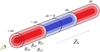 |
Fig. 3. Illustration of the K-estimator. We show three nested cylinders representing three bins of transverse separations. The number of galaxy pairs inside each blue cylindrical shell from a1 = 0 to ±a2 is N0, a2, the number of pairs in each red cylindrical shell between a3 − a2 and −a2 − ( − a3) is Na2, a3. The K-estimator for each shell is then the ratio of pair counts between the inner (blue) segment to the total (blue plus red) segment. For illustration purposes we depict linear Rij bins, although in practice we use a logarithmic binning scheme. |
The transverse distance Rij between LAE pairs is taken in bins of Rij, corresponding to different cylindrical shells in Fig. 3. These shells are defined by their radii Rij and their lengths a2, a3 in the Z direction. For illustration purposes, we display Rij in Fig. 3 using a linear scaling (Rij2 − Rij1 = Rij3 − Rij2 etc.), although in practice we adopt a logarithmic spacing of subsequent transverse separations. We note that in this figure each Rij and Zij combination corresponds to a galaxy pair and not just a single galaxy.
 is related to the 2pcf through the mean value of the correlation function
  (see Adelberger et al. 2005)
![Mathematical equation: $$ \begin{aligned} \langle K_{a_2, a_3}^{a_1, a_2}(R_{ij}) \rangle \simeq &{(a_2-a_1) \cdot \displaystyle \sum _{i>j}^{\mathrm{pairs}}[1 + \overline{\xi }{_{a_1, a_2}}]}\nonumber \\&\times \left\{ (a_2-a_1) \cdot \displaystyle \sum _{i>j}^{\mathrm{pairs}}[1 + \overline{\xi }{_{a_1, a_2}}]\right.\nonumber \\&\qquad \quad \left.+ (a_3-a_2) \cdot \displaystyle \sum _{i>j}^{\mathrm{pairs}}[1 + \overline{\xi }{_{a_2, a_3}}]\right\} ^{-1}, \end{aligned} $$](/articles/aa/full_html/2021/09/aa41226-21/aa41226-21-eq12.gif) (2)
(2)
where  is
is
 (3)
(3)
and corresponds to the mean correlation function that would be theoretically measured in the blue region in Fig. 3. The same is applied for  in the red region of Fig. 3. The function ξ(Rij, Zij) can be represented by a power law through the Limber Equation (Limber 1953) in spatial coordinates
  or modelled with a halo occupation distribution model.
The understanding of this estimator is quite intuitive. If galaxies were randomly distributed in space (ξ(r) = 0), the expected number of galaxy pairs at each LOS separation would be equal. Thus, from Eq. (2) and with a1 = 0,  is simply the ratio of volumes between the two cylindrical shell segments, (a2 − 0)/(a2 − 0 + a3 − a2) = a2/a3. Hence if a3 = 2a2, the expectation value for an unclustered galaxy population would be K = 0.5; if for a specific sample the value of K is significantly above 0.5, we have detected a clustering signal. We note, however, that while this criterion (applied by both Adelberger et al. 2005; Diener et al. 2017) seems natural, there is no a priori reason to keep the restriction to a3 = 2a2. In fact, allowing for a3/a2 > 2 provides the analysis with a more solid statistical baseline against which the clustering signal can be evaluated (addressed in Sect. 3.1.2).
Adelberger et al. (2005) applied Eq. (2) and the Limber equation to estimate the correlation length, r0, while keeping the power law slope γ of the correlation function fixed. They first measured the K-estimator in a single Rij bin Rcut < 5 h−1 Mpc which captures the Rij scale for which the clustering signal is largest. They then applied Eqs. (2) and (3) to predict the expectation values ⟨K⟩ for different assumed values of r0, selecting the correlation length for which the predicted value of K was closest to the measured value as their best estimate. The same procedure was adopted by Diener et al. (2017) in their analysis of a MUSE-Wide subset of LAEs. We refer to this approach in the following as the ‘one-bin fit’ method.
In addition to this simple approach to estimate r0 at fixed γ, we also implemented a more elaborate procedure to fit the K-estimator with a power law correlation function with both γ and r0 as free parameters. For this purpose, we integrate ξ(r) over both Zij ranges as in Eq. (3), for each Rij bin and for each combination of a grid in (r0, γ). Plugging the values of these integrals into Eq. (2) to calculate ⟨K⟩ for each Rij bin, we obtain a global χ2 value for each grid point by summing over the squared deviations between predicted and observed values of K relative to the statistical error bars (obtained by bootstrapping as explained in Sect. 3.1.3). Our best-fit parameters are then finally taken as the (r0, γ) grid point with the smallest χ2. For the estimation of confidence intervals, we face the complication that the K values in subsequent Rij bins are correlated because each galaxy contributes to multiple pairs at various separations. We explain in Sect. 3.1.3 how we obtained realistic uncertainties for the fit parameters.
3.1.2. Optimizing the K-estimator
The parameters a2 and a3 in the definition of the K-estimator can in principle be chosen freely. We now explore for which values we obtain the best sensitivity for the clustering signal and the highest signal-to-noise ratio (S/N). We compute the S/N from the error bars of the correlation lengths. This procedure is similar to finding the optimal πmax saturation value in the case of the 2pcf, where πmax is increased until most of the correlated pairs are included, while even larger values of πmax only add noise to the measurement.
We performed a grid search with the full sample over the different combinations of  , but setting a1 = 0 throughout. Here, we vary a2 within 5−25 h−1 Mpc in steps of 2 h−1 Mpc and a3 within 5−50 h−1 Mpc in steps of 5 h−1 Mpc, with the additional restriction a3 ≥ a2. We adopt 15 logarithmic bins in the range 0.6 < Rij < 12.8 h−1 Mpc, discarding Rij bins with fewer than 16 galaxy pairs. We use the one-bin fit described above with a fixed canonical γ value of γ = 1.8 (Adelberger et al. 2005; Durkalec et al. 2014; Ouchi et al. 2017) to calculate the correlation length, r0, and the S/N for each combination (a2, a3).
The results are shown in Fig. 4. The left panel reveals that the S/N is highest for small a2 and large a3 values, while it decreases towards a2 ≈ a3. Parameter combinations with a2 = a3/2 as adopted in the two previous studies that used the K-estimator (Adelberger et al. 2005; Diener et al. 2017) are represented by the colored circles; it is evident that these combinations are far from optimal with regard to bringing out the clustering signal with maximal significance.
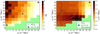 |
Fig. 4. Results of our grid study to optimize the K-estimator. Left: S/N obtained for each evaluated combination of (a2, a3), displayed as a color map. The green area indicates the ‘forbidden’ range where a3 < a2. The contours trace S/N increments of 2, slightly smoothed for display purposes. Right: same parameters but for the correlation length r0, except that the contours again follow the values of the S/N. The blue-red colored circles represent grid points with a3 = 2a2 for which the blue-red cylinders in Fig. 3 are equally long. The blue cross indicated our adopted parameter combination for the clustering analysis, as it provides the highest S/N and reaches saturation at r0. |
The right panel of Fig. 4 shows that in the upper left range of the diagram where the S/N is highest, the best-fit value of r0 is also insensitive to the specific parameter combination. On the other hand, larger values of a2 and smaller values of a3 degrade the S/N. Comparable a2 and a3 values (tiny red and large blue cylinders in Fig. 3) result in Na2, a3(Rij) < < Na1, a2(Rij), with Na2, a3(Rij) strongly varying with the exact value of a3. This translates into large uncertainties when computing r0 from the K-estimator (see Eq. (1)). These errors are however not reflected in the right panel of Fig. 4 but are clearly visible in the low S/N on its left panel. The largest r0 values therefore correspond to the most uncertain values but agree well within their uncertainties with the r0 value accepted by us. We adopt the combination a2 = 7 h−1 Mpc and a3 = 35 h−1 Mpc, marked with a blue cross in both plots, for the rest of this paper as the grid point giving the highest S/N and a r0 within the saturation values. Thus, in the following, we always refer to the specific estimator  which quantifies the ratio of the number of galaxy pairs with LOS separations between −7 < Zij/h−1 Mpc < 7 and between −35 < Zij/h−1 Mpc < 35 at given transverse distance Rij. The expectation value of this estimator for an unclustered population is (a2 − a1)/(a3 − a1) = 0.2.
3.1.3. Error estimation
The individual data points from clustering statistics are correlated. One galaxy can contribute to galaxy pairs in more than one Rij bin. In order to account for this correlation one would use the jackknife resampling technique and compute a covariance matrix (see e.g. Krumpe et al. 2010). However, that method requires a division of the sky area into several independent regions, each of which must be large enough to cover the full range of scales under consideration. Due to the small sky area of our survey, this approach is not feasible here. Poisson uncertainties, even if commonly used, might underestimate the real uncertainties. We therefore consider several alternatives to derive meaningful uncertainties in Appendix C and choose the most conservative approach.
Thus, we apply the bootstrapping technique detailed in Ling et al. (1986) (and similar as in Durkalec et al. 2014) to determine the statistical uncertainties of our data points. We create pseudo-data samples by randomly drawing 695 LAEs from our parent sample, allowing for repetitions. We generate 500 different pseudo-samples and compute the K-estimator in all of them. The standard deviations of K in each Rij bin are adopted as error bars. We verify the robustness of our error approach in Appendix C.
With the bootstrapped uncertainties and the uncorrelated χ2 statistics, the uncertainties of the clustering parameters can be derived. However, we suspect that naively applying an uncorrelated χ2 analysis with the standard confidence threshold can also lead to an underestimation of the clustering uncertainties. Therefore, we test this hypothesis by investigating the behavior of the error bars when the bin size is modified. While we would generally expect a decrease in the individual uncertainties when the bin size is increased, here we expect an increase in the error bars if the bin size is decreased.
We compute new bootstrapping error bars for five different Rij bin sizes (half size, double size, three times larger, four times larger and five times larger than the current binning). The error bar sizes do not vary significantly when the Rij bin size is modified, contrary to the expectation of the standard χ2 method.
We therefore recalibrate the χ2 analysis to determine realistic 68.3% and 95.5% confidence levels in the following way: with each of our bootstrapped samples delivering a best-fit minimal value of  corresponding to (r0, i, γi), we assume that the posterior distribution of these
  approximately describes the true confidence regions. We compute the
  values using the corresponding (r0, i, γi) combinations and our real data. We sort these
  into ascending order and adopt the 68.3% and 95.5% parameter ranges with respect to the sorted bootstrapped
  values as marginalized single-parameter error bars. This posterior distribution is also used to provide combined confidence regions on both r0 and γ. Throughout the paper, we refer to this fitting approach as a ‘PL-fit’.
3.2. Two-point correlation function
The 2pcf is undoubtedly the most frequently used statistic to investigate galaxy clustering. Although we argued above that it is less suited than the K-estimator for a pencil-beam survey such as MUSE-Wide, we include a 2pcf analysis of our sample for comparison in Appendix D. We note that this is in fact the first time that such an analysis has been performed on a 100% spectroscopically confirmed sample of LAEs. However, the challenge of estimating realistic uncertainties in the case of the 2pcf is even more problematic (due to the survey design) than for the K-estimator. We present in Appendix D an in depth presentation and discussion of the 2pcf on our LAE sample. In summary, we show that the results from the K-estimator and 2pcf agree within their uncertainties.
3.3. Bias and typical Dark Matter Halo masses from power-law fits
The clustering strength is characterized by the large-scale bias factor b, which relates the distribution of galaxies to that of the underlying dark matter density. The bias factor has often been derived from the characteristic correlation length r0 and the PL slope γ by fitting a PL to the clustering signal (e.g. Peebles 1980). Given b, we can also derive typical host DMH masses. Within the concept of linear bias, the evolution of b with redshift is given by the ratio of the density variance of galaxies σ8, gal(z) over that of dark matter σ8, DM(z):
 (4)
(4)
For a power-law 2pcf the relation between ξ(r) and the density variance σ8, gal(z) (Peebles 1980; Miyaji et al. 2007) is given by
 (5)
(5)
where ξ(r8, z) is the correlation function evaluated in spheres of comoving radius r8 = 8 h−1 Mpc and J2 = 72/[(3 − γ)(4 − γ)(6 − γ)2γ]. Simultaneously, for the DM case:
 (6)
(6)
with D(z) as the linear growth factor.
Inserting Eqs. (5) and (6) into Eq. (4) we obtain the bias factor as a function of the growth factor
![Mathematical equation: $$ \begin{aligned} b(z) = \left[\frac{r_8}{r_0(z)}\right]^{-\gamma /2} \frac{J_2^{1/2}}{\sigma _8 D(z)/D(0)}\cdot \end{aligned} $$](/articles/aa/full_html/2021/09/aa41226-21/aa41226-21-eq28.gif) (7)
(7)
Following the bias evolution model described in Sheth et al. (2001), we can compute the large-scale Eulerian bias factor bEul and compare it to the bias given by Eq. (7) in order to estimate DMH masses. To calculate bEul, we consider linear overdensities in a sphere which collapses in an Einstein-de Sitter Universe at δcr = 1.69. The linear root mean square fluctuations correspond to the mass at the epoch of observation ν = δcr/σ8, DM(MDMH, z). The theory behind the σ8, DM(MDMH, z) calculation is developed in Van Den Bosch (2002).
3.4. Halo occupation distribution modelling
It is known that bias factors and DMH masses inferred from PL fits suffer from systematic errors (e.g. Jenkins et al. 1998 and references therein). A PL correlation function treats scales in the linear and non-linear regime alike and does not differentiate between pairs of objects belonging to the same DMH and pairs residing in different halos. Even for fits performed only in the linear regime, the correlation function still deviates from the PL shape. A more appropriate treatment is achieved through HOD modelling that explicitly combines the separate contributions from the one- and the two-halo terms.
The HOD model we use here is an improved version of the model set presented by Miyaji et al. (2011), Krumpe et al. (2012, 2015, 2018). To maintain consistency with these studies, we use the bias-halo mass relation from Tinker et al. (2005), the halo mass function of Sheth et al. (2001), the dark matter halo profile of Navarro et al. (1997), and the concentration parameter from Zheng et al. (2007). We use the weakly redshift-dependent collapse overdensity δcr (Navarro et al. 1997; Van Den Bosch et al. 2013). We further include the effects of halo-halo collisions and scale-dependent bias by Tinker et al. (2005) as well as redshift space distortions using linear theory (Kaiser infall, Kaiser 1987; Van Den Bosch et al. 2013) to the two-halo term only (see Appendix E).
The mean occupation function is a simplified version of the five parameter model by Zheng et al. (2007), where we fix the halo mass at which the satellite occupation becomes zero to M0 = 0 and the smoothing scale of the central halo occupation lower mass cutoff to σlog M = 0.
In this simplification, the mean occupation distribution of the central galaxies can be expressed by
 (8)
(8)
and that of the satellite galaxies ⟨Ns(M)⟩ as
 (9)
(9)
where Mmin is the mass scale of the central galaxy mean occupation, M1 is the mass scale of a DMH that hosts (on average) one additional satellite galaxy, and α is the high-mass slope of the satellite galaxy mean occupation function.
We apply the model to obtain the ξ(r) based on HOD modelling and convert the calculated ξ(r) to the K-estimator using Eq. (2). The minimum transverse separation of our observed K-estimator is ∼0.6 h−1 Mpc, where the one-halo term contribution to ξ(r) is typically a few to several percent. This is too low for obtaining robust constraints on the one-halo term to perform a full HOD modelling. We therefore restrict our analysis to an estimate of the bias parameter by fitting the expected K-estimator based on only the two-halo term to the observations. We hold α = 1 and log M1/Mmin = 1 fixed and vary only Mmin to find the best-fit model and calculate the bias parameter. This probes the typical DMH mass for the sum of central and satellite galaxy halo occupations, N(Mh) = Nc(Mh)+Ns(Mh), without being able to distinguish between these two.
The details of the HOD models (e.g. M1 and α) do not affect the typical DMH mass estimations since we only fit the two-halo term. Some HOD modelling applications in the literature also use number density constraints (e.g. Eq. (18) of Miyaji et al. 2011). This is, however, only relevant if the one-halo term contributes significantly, which is not the case here. Thus, we do not need to employ any number density constraints. The HOD model is evaluated at the median redshift of N(z)2 where N(z) is the redshift distribution of the sampled galaxies. For our dataset, zpair = 3.82.
As above for the PL-fit parameters (Sect. 3.1.3), we estimate the uncertainties of the inferred bias factor by fitting the 500 bootstrapped samples with the two-halo term HOD modelling and obtain the 500 best bias factors from the bootstrapped samples. Those best 500 HOD models are then compared to the observed K-estimator data points to compute the bootstrapped χ2 values. We sort the bootstrapped  values in ascending order and use these to recalibrate the 68.3% (1σ) confidence interval.
4. Results
4.1. K-estimator
Adopting the optimized K-estimator  (see Sect. 3.1.2), we measure the clustering of our LAE sample in 15 logarithmic bins of transverse separations Rij between 0.6 and 12.8 h−1 Mpc, with error bars calculated by bootstrapping the sample as explained in Sect. 3.1.3.
Figure 5 shows the results for the full LAE sample. It is evident that the values of K are significantly above the no-clustering expectation value of 0.2.
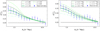 |
Fig. 5. Measured values of the K-estimator as a function of transverse distance (points with error bars) compared to the expected behaviour for a population strictly following a power-law correlation function. Left: five curves represent different power-law indices as given in the legend, for a fixed value of r0 = 3.6 h−1 Mpc. Right: same details for five different correlation lengths at fixed γ = 1.3. The central (thick solid) curves always indicate the minimum χ2 best-fit values. The horizontal straight line shows the no-clustering expectation value of K. The error bars are calculated with the bootstrapping technique described in Sect. 3.1.3. |
We can verify that our clustering results are not affected by the accuracy of our redshifts (see Appendix B), also taking into account our statistical corrections for the expected offset between Lyα-based and systemic redshifts (see Sect. 2.2). We emphasize that the K-estimator is insensitive to these redshift errors because of the broad (±7 h−1 Mpc) window over which the numerator in Eq. (1) is evaluated.
A somewhat puzzling feature, at least at first sight, is the broad hump in the K(Rij) profile around 4 ≲ Rij/h−1 Mpc ≲ 7, suggesting a slight excess in the clustering strength for such separations (or alternatively, a dent at 2 ≲ Rij/h−1 Mpc ≲ 4). We test the possibility that this feature might be introduced as an artefact of the sample footprint shape by dividing the sample into an ‘eastern’ and a ‘western’ half. Since we find the hump (or dent) in both subsets, as is also the case when splitting the sample by LAE properties (see Sect. 5), we rule out a systematic effect due to the footprint. Recalling the fact that the data points in Fig. 5 are strongly correlated, we underline that the significance of the feature is actually below 2σ, and we consider it to most likely be due to a statistical fluctuation in the spatial distribution of the sample. The only robust test of this explanation would require an independent but statistically equivalent comparison sample, which we do not have at our disposal. However, we removed the data points of the hump or dent and tested the possible effect of this feature on our fits to the K-estimator. We find the same clustering parameters (within 1σ) as in the next section. For the purpose of this paper we treat the hump or dent as an insignificant statistical fluctuation that is not related to a true clustering excess of the MUSE-Wide LAEs.
We also checked that our clustering signal is insensitive to including or excluding the objects from the 8 HUDF09 parallel fields (Δb = 0.03; see Appendix A), again confirming the robustness of the K-estimator on the survey footprint.
4.2. Power law fits
First, we applied the single-bin fit method to our clustering signal to compare our results to earlier studies, which also computed the K-estimator and evaluated its strength by using the single-bin fit approach. We derived the best-matching correlation length r0 at fixed γ = 1.8, as described in Sect. 3.1.1. The calculated value of  for Rij, max < 5 h−1 Mpc corresponds to r0 = 2.10 ± 0.20 h−1 Mpc. The outcome of this single-bin fit depends somewhat on the adopted Rij, max: lowering the limit to 3 h−1 Mpc results in
  Mpc, whereas increasing Rij, max to 7 h−1 Mpc delivers
  Mpc. In principle, this dependence should be included in the error bar on r0. We also vary the fixed value of γ between 1.0 and 2.0 and find that r0 does not change by more than 1σ. Our single-bin fit results agree with those in Diener et al. (2017) but give much tighter constraints on r0.
Motivated by these results we proceed to estimate both parameters simultaneously. Since in the single-bin approach the choice of Rij, max does affect the fit result, we now switch to fitting the K-estimator over the full measured range of transverse separations using all bins in 0.6 < Rij/h−1 Mpc < 12.8 (see Sect. 3.1).
To obtain a visual impression of how  depends on γ and r0 separately, we overplot the expected curves for five different values of each quantity into Fig. 5, always keeping the other parameter fixed. It can be seen that K reacts in different ways to changes in the two parameters. Increasing r0 leads to an elevated K at all Rij scales, whereas increasing γ results in changes of K mainly at small transverse separations. Because the shape of
  changes differently for r0 and γ, it is in principle possible to fit both parameters simultaneously. We perform an uncorrelated χ2 analysis over a grid of r0 and γ to find the best-fit parameters as described in Sect. 3.1.1.
Following the procedure laid out in Sect. 3.1.3 we compute confidence contours for r0 and γ by fitting the 500 bootstrapped samples in the same way. The marginalized single-parameter (1D) 16%−84% confidence regions are  and
and  . These and the corresponding 2-dimensional 68.3% and 95.5% confidence contours are displayed in Fig. 6, along with the 500 best-fit parameter sets from the bootstrapped pseudo-data samples. For a visual comparison we also plot the estimations from the single-bin fit. We further include the results from a one-parameter PL-fit with fixed γ = 1.8 for an easier comparison with the literature in Sect. 5.2.
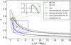 |
Fig. 6. Simultaneous fit to r0 and slope γ. The black (dark grey) contour represents the 68.3% (95.5%) confidence. The red cross stands for the lowest χ2 value at (r0 = 3.65, γ = 1.25). The points show the 500 best-fit values from the 500 bootstrapped samples. The blue rectangle indicates the 16% and 84% percentiles from the marginalized single-parameter posterior distributions of the bootstrapped samples. The green (red) error bar represents the correlation length from the one-parameter PL (single-bin) fit with fixed γ = 1.8. For a better visualization, we show a zoom onto the region containing these fits. |
The best-fit correlation length of 2.1 h−1 Mpc obtained by the single-bin fit (at fixed γ = 1.8) is lower than suggested by the one- and two-parameter fits and it is not compatible with its 68.3% probability contour. This was expected because the single-bin fit was not optimized for r0, S/N and Rij range. We also observe a large similarity between the medians of the marginalized single-parameter posterior distributions ( Mpc,
Mpc,  ) and the combination of parameters that provide the lowest χ2 value (r0 = 3.65, γ = 1.25). It is also evident from Fig. 6 that the fit is quite degenerate between r0 and γ in the sense that parameter combinations with higher γ and lower r0 are only slightly less likely than the best-fit combination. Different Rij scales are affected when modifying γ or r0 (see Fig. 5). This results in similarly good PL-fits when combinations of low γ and high r0 or high γ and low r0 are applied. Taking into account the sensitivity of the single-bin fit to the value of Rij, max, the three results are in fact very similar. We therefore adopt the PL fitting approach also for our subsequent investigation of the dependence of clustering on LAE physical properties. This eases the comparison to the literature, where mainly PL fits are performed. The values and errors of the best-fit parameters from the different fit approaches are summarized in Table 2.
Clustering parameters from the different fit approaches to the K-estimator in our full sample.
The confidence contours of our fit are essentially open towards large r0 and low γ. In fact, our bootstrap sample contains a sizeable proportion of instances with best-fit combinations in the lower right corner of Fig. 6 (11.8% with r0 > 10 h−1 Mpc). Upon investigation of these ‘solutions’, we find that they correspond to almost constant K-estimator values with respect to Rij, driven by the tentative hump around 5 h−1 Mpc. Whatever the actual origin of these extreme points, it seems clear that from the K-estimator alone without further priors we can only constrain plausible combinations of r0 and γ at one end of the distribution.
While it appears that the best-fit power-law index for our LAEs tends to be substantially shallower than the results from other studies based on NB imaging that use the fiducial γ value of γ = 1.8 (e.g. Ouchi et al. 2010, 2017), we note that they are generally compatible at the 1−2σ level. The same is true for the values obtained from our own sample using the 2pcf method (see Appendix D).
4.3. Halo occupation distribution fit
We can then match the HOD model (Sect. 3.4) to our measured K-estimator. Similarly to Fig. 5 we first visualize the basic behaviour of the HOD model for different large-scale bias factors (shown in Fig. 7). Higher values of b increase the expectation values of K at most separation scales, but most strongly for small Rij. Following the procedure described in Sect. 3.4 we recalibrate the confidence contours and obtain a best-fit large-scale bias of  . The corresponding typical DMH mass is
 ![Mathematical equation: $ \log (M_{\mathrm{DMH}}/[h^{-1}\,M_\odot]) = 11.34^{+0.23}_{-0.27} $](/articles/aa/full_html/2021/09/aa41226-21/aa41226-21-eq52.gif) .
.
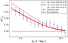 |
Fig. 7. Dependence of the HOD fits to the K-estimator on the large-scale bias factor. The dotted, solid, and dashed red curves show three different bias factors b = 2.3, 2.8, 3.3, respectively. The thicker solid red curve shows the b that provides the lowest χ2 value. The K values and their respective error bars are the same as in Fig. 5. |
The best-fit HOD model behaves in several aspects similarly to the best-fit PL correlation function. Even if PL fits do not have a physical basis, the PL model seems to perform slightly better in terms of matching the observed K values and reaching a slightly lower χ2 value, but these differences are not significant. The bias values derived from the two fits are also fully consistent as discussed in Sect. 5.3.
We investigate the effects of the redshift space distortions (RSD) in Appendix E, where we show that the RSD do not have a significant effect on the HOD fit for K-estimator.
5. Discussion
5.1. Comparison to Diener et al. (2017)
We first compare our results with those of our pilot study (Diener et al. 2017, D17) which employed the non-optimized K-estimator  for a subset of 24 fields of our current sample. In order to visualize the statistical gain of our new investigation, we applied our improved
  estimator to the 196 LAEs at 3.3 < z < 6 in the same 24 fields. The outcome of this comparison is shown in Fig. 8.
 |
Fig. 8. Measured values of the K-estimator of our sample of 68 MUSE-Wide fields (blue filled circles) compared to the subset of 24 fields considered in Diener et al. (2017, D17; open red circles). The error bars are again calculated with the bootstrapping technique described in Sect. 3.1.3. The blue dotted curve represents our two-parameter best PL-fit. The red dotted curve uses the best single-bin fit results of D17 ( |

While the two datasets show excellent agreement given the uncertainties, as expected the error bars are much smaller in our new sample. The clustering signal of the 24 fields appears a bit higher, but the differences are at most 1σ. The smaller footprint of the 24 fields dataset limits the range of transverse separations ≲6 h−1 Mpc. The clustering curves from the two samples are fitted with a PL correlation function, based on the results from D17 for the 24 fields and on our best PL-fit for the 68 fields. Figure 8 also shows that the power-law fits to the 68 fields follow the data points much better than in the 24 fields since we performed a simultaneous fit of r0 and γ. Following the same procedure as in Sect. 3.1.3 for the 24 fields, we find  Mpc and
  . These results are very close to the numbers obtained in D17 (
 cMpc for a fixed γ = 1.8), but our improved procedure substantially decreased the error bars for the same data.
5.2. Comparison with the literature
Most previously published works on the clustering of high-redshift galaxies are restricted to the estimation of r0 at fixed power-law index γ, with the latter typically assumed to be 1.8 or thereabouts. While our best-fit value for γ based on the K-estimator is considerably lower, Fig. 6 shows that γ values around 1.8 are still consistent with our data. To make a fair comparison, in Sect. 4.2 we recompute the best-fitting power law with γ fixed to 1.8; thus only allowing r0 to vary.
Furthermore, the clustering strength and thus the correlation length are predicted to evolve with cosmic time and, thus, the (average) redshifts of the samples must also be taken into account in any comparison.
We first considered clustering measurements of LAEs selected by NB surveys. Here, all objects are assumed to have the same redshift defined by the NB filter. Early studies (Ouchi et al. 2003; Gawiser et al. 2007; Shioya et al. 2009) focused on small samples of LAEs (up to 160 objects) at z = 3.1 − 4.86 to compute angular correlations. The correlation lengths at fixed γ = 1.8 (except Shioya et al. 2009, who calculated γ = 1.90 ± 0.22) are consistent with our recomputed PL-fits, in particular when considering the involved uncertainties. The correlation lengths are in the range of r0 ≈ 2.5 − 4.5 h−1 Mpc, higher values corresponding to higher redshift samples. More recent studies based on NB surveys (Ouchi et al. 2010, 2017; Bielby et al. 2001) at higher redshifts (z ≈ 3 − 6.6) hold much larger samples (up to 2000 objects), where they find slightly higher correlation lengths, r0 = 3 − 5 h−1 Mpc. Given the similarity between these and lower redshift samples, our derived correlation lengths are also in fair agreement with most recent LAE clustering studies.
We then considered clustering measurements of high-redshift galaxies selected based on photometric redshifts or magnitude and colour-colour criteria (mainly Lyman-break galaxies). Durkalec et al. (2014, 2018) computed the real-space 2pcf on samples of more than 3000 objects at 2 < z < 5 distributed over more than 0.8 deg2. The sample is more suited for clustering studies than our MUSE-Wide survey because their large spatial coverage diminishes the effect of cosmic variance and allows the computation of the traditional 2pcf method. Thanks to the characteristics of the survey they perform a two-parameter PL-fit and derive a correlation slope of  and a correlation length of
  Mpc at z ∼ 2.5. At z ∼ 3.5 they obtain lower slopes
  and higher lengths r0 = 4.35 ± 0.60. Our results not only agree with their clustering parameters but also point toward a lower slope for higher redshift galaxies. Moustakas & Somerville (2002) also reported a redshift dependence of γ; in addition, the authors parameterized analytically the correlation slope as a function of redshift.
Figure 9 compiles the comparison of correlation lengths from the literature and those derived in this work with different fit approaches. We also plot the correlation lengths for our redshift subsamples (see Sect. 5.4).
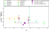 |
Fig. 9. Comparison of the derived correlation lengths to the literature. The r0 values calculated in this study are represented with purple stars. Green symbols correspond to studies of samples based on Lyα selected galaxies. The samples from Durkalec et al. (2014) at z ∼ 2.5 and z ∼ 3.5 (dark and light yellow) are based on continuum-selected high-z galaxies. The horizontal colored bars indicate the redshift ranges of the corresponding studies (spectroscopic surveys). The redshift range of the z-subsamples of this paper are not plotted for a better visibility. Values for r0 are plotted at the median redshift of the samples. The r0 from Ouchi et al. (2003) and Bielby et al. (2001) have been shifted by +0.1 along the x-axis for visual purposes. Our one-parameter PL-fit with fixed γ = 1.8 by +0.2. The upper limit of the r0 from Shioya et al. (2009) corresponds to r0 = 10.1 Mpc. |
Most literature values are in agreement with our findings, both with the r0 from the two-parameter PL-fit and from the one-parameter PL-fit with fixed γ = 1.8 ( h−1 Mpc). Not surprisingly, given the r0 dependence on Rij, max, the value from the single-bin fit is lower than in most studies (including our robust PL-fit approach results).
A more appropriate but not so traditional comparison of the clustering strength is the bias factor, derived from γ and r0 (for PL-based correlation functions) or from HOD models. At z ∼ 3 Bielby et al. (2001) reported a bias factor of bPL = 2.13 ± 0.22 and DMH masses of MDMH = 1011 ± 0.3 h−1 M⊙, whilst at the same redshift, Durkalec et al. (2014) reported a somewhat larger bias value of bHOD = 2.82 ± 0.27 and typical DMH masses of log(MDMH/h−1 M⊙) = 11.75 ± 0.23. As for Ouchi et al. (2017), they obtained a bias value of  and typical DMH masses of log
 at z = 5.7, whilst Ouchi et al. (2010) derived bias values in the range b = 3 − 6 and typical DMH masses of MDMH = 1011 ± 1 h−1 M⊙ at z = 6.6. Our results fall between the values derived from studies at z = 3 and z = 5.7.
Each study, however, probes different luminosity and EW ranges, an effect that may have an impact on the interpretation of the clustering results from the literature. Despite these differences, it is interesting to note the general agreement in the clustering parameters from the different studies at similar z. Consequently, the hosting DMH mass of galaxies are also very similar. We present our testing of the sample, aimed at characterizing such dependencies, in the next section.
5.3. PL vs. HOD fits
The various fit methods performed on the K-estimator allow us to compare the derived PL-fit results to those from HOD modelling. We tested the performance of the different PL-fit approaches and we developed an improved fit method.
The clustering signal provided by the K-estimator was never robustly fitted in previous studies (Adelberger et al. 2005; Diener et al. 2017). The correlation length r0 was obtained by measuring the K-estimator in a single Rij bin (Rcut < 5 cMpc) and comparing the result to the expectation values ⟨K⟩ provided by Eq. (2) for different correlation lengths. In the process, a PL correlation function of fixed slope was assumed but never directly fit to the K-estimator. Instead, the correlation length that yields the closest match between ⟨K⟩ and Kmeasured was chosen as the best correlation length. However, in Sect. 4.2, the result varies significantly depending on the chosen Rcut. Due to the simplicity of this approach and its dependence on Rcut, we fit the measured K-estimator as a function of Rij with the model predictions (Eq. (2)), providing a more reliable and accurate fit to the full Rij range covered by the K-estimator.
Taking the K-estimator one step further, we also make use of HOD models. As explained in Sect. 3.4, PL-based correlation functions do not distinguish between the one- and two-halo term regimes. PLs are just an approximation, whereas HOD models treat galaxies residing in one DMH and in different DMHs differently, being a more advanced and physically meaningful approach.
We measure the clustering only at Rij > 0.6 h−1 Mpc so we do not cover the one-halo term of the correlation function. Hence, we fit the two-halo term of ξ(r) from the HOD model to our K values in order to obtain the large-scale bias of our sample.
In Fig. 10 we show both PL and HOD best-fits to the K-estimator from the χ2 analysis described in Sect. 3.1. The performance of the curves is comparable and there are only tiny variations in the shape of the curves. Nonetheless, the PL-fit achieves the lowest χ2, indicating a modest better performance.
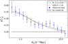 |
Fig. 10. Best PL and HOD fits to the K-estimator. The dashed green curve shows the PL-fit (same as the solid curves in Fig. 5) while the dotted red curve represents the HOD fit (same as the thick curve in Fig. 7). The measurements of |

Even though the curves are nearly identical at intermediate separations (1 < Rij/h−1 Mpc < 2.5), at smaller and larger separations, the curves deviate from each other. The largest difference occurs at small separations (Rij < 1 h−1 Mpc), where the PL flattens but the HOD fit continues to increase. Less remarkable is the difference at large separations (Rij > 2.5 h−1 Mpc), where the PL-fit is somewhat higher than the HOD fit. In both cases, the differences are well within the uncertainties, and in the main range used to calibrate the bias factor (Rij > 1 h−1 Mpc), the variations between the fits are minute.
We show the comparison between the large-scale bias parameters calculated from the PL and HOD fits listed in Tables 2 and 3 in Fig. 11. The derived bias factors from the PL fits are slightly higher than the HOD values, while the HOD uncertainties are, on average, smaller (≈25%) than those from the PL fits. Using samples of AGN and a cross-correlation function approach, Krumpe et al. (2012) also compared PL and HOD clustering fits. They found higher bias factors and smaller uncertainties from the HOD fits because they included part of the one-halo term in the PL fit. As we have explained, strong variations between samples in the one-halo term cause a decrease in the bias factors derived from the PL fits. However, we do not include the one-halo term in any of our fits so we are not subjected to these variations.
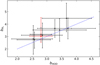 |
Fig. 11. Comparison between the bias parameters derived from the PL and HOD fits listed in Tables 2 and 3. We highlight the bias factor from the full sample of LAEs with a red square. The dotted blue line shows a 1:1 correspondence. |
Derived clustering parameters from the subsamples.
5.4. Clustering dependence on physical properties
We searched for clustering dependencies on LAE physical properties. We computed the K-estimator in the subsamples described in Sect. 2.3, but the lower number of objects in the subsets does not allow for a two-parameter PL-fit. We therefore take the prior from our full sample and assume that our subsamples present the same correlation slope as the parent sample (γ = 1.3). We then performed the one-parameter PL-fit with fixed γ = 1.3. We also conducted HOD fits in the same way as we did for the full sample.
5.4.1. Redshift
Taking advantage of the large redshift range provided by MUSE, we investigate whether LAEs occupy denser regions of the Universe at earlier epochs by measuring their clustering strength with the K-estimator.
At the cost of enlarging the error bars (and as explained in Sect. 2), we split our sample in two bins around the median redshift, ⟨z⟩ = 4.12. We computed the K-estimator in both subsamples, with the results given in the top left panel of Fig. 12.
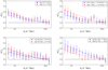 |
Fig. 12. Clustering dependencies on object properties. Top left: clustering variation in two different redshift subsamples. The blue dots show the clustering in the lower redshift bin while the red points show the higher redshift subsample. The dotted curves represent the best HOD fits. Top right: same details but for two different Lyα luminosity subsamples. Bottom left: same details but for EWLyα. Bottom right: same details but for UV absolute magnitude. The black line represents the K expectation value for an unclustered sample of galaxies and the 1σ error bars are determined from the bootstrapping approach explained in Sect. 3.1.3. |
The two curves are essentially indistinguishable within the error bars. Both follow the same trend and have similar shapes. Analogously to Sect. 4.2, we fit a PL correlation function ξ(r) = (r/r0)−γ with fixed slope γ = 1.3. For the low redshift subsample, we obtain  . The resulting value for the high-redshift bin is
  . The best-fit parameters are listed in Table 3 along with the bias factors obtained from the HOD fit and their corresponding DMH masses.
The difference between the best-fit parameters (lower than 1σ) of the subsamples do not allow us to corroborate or contradict the general statement “LAEs reside in more massive DMHs at higher redshifts”. However, other studies found higher bias factors of LAEs at higher redshifts (e.g. Ouchi et al. 2010). Even if the study of samples at fixed luminosities is needed, this has been interpreted as evidence for downsizing, with galaxies residing in the largest DMHs going through their ‘LAE phase’ early in the Universe, while Milky Way progenitors appear as LAEs at later times, around z ∼ 3.
We confirm that our findings are not strongly affected by the selected redshift cut of the sample. Varying the cut by 10% in z, from z = 4.12 to z = 4.53, changes the number of LAEs in each subsample by ∼15% (118 objects) and results in an increase in b within 1σ, which is equivalent when considering the uncertainties; whereas, the z and LLyα values are not independent. Therefore, the different luminosity distributions in the different redshift subsamples may bias the detection of a clustering dependence on redshift. To assure that the investigation of the clustering dependence on z is not driven by the different LLyα distributions, we apply a ‘matching’ technique similar to Coil et al. (2009) and Krumpe et al. (2015). To do so, we compare individual bins between the two luminosity distributions of the z-subsamples. In each bin, we check which subsample contains more objects. We then select the one with the higher number and randomly remove objects until we match the number counts of the other subsample in that bin.
Once the two luminosity distributions are equivalent, we run the K-estimator in both subsamples with now matched LLyα distributions but still different redshift distributions. We find fully consistent results when making a comparison with our original subsample definition. The clustering difference between the ‘matched’ and ‘unmatched’ subsamples varies within 1σ. Therefore, we discard the possibility of a possible clustering dependence on z driven by LLyα as well as a strong clustering dependence on z.
5.4.2. Lyα luminosity
To learn about the DMHs where LAEs of different Lyα luminosities reside, we studied the clustering dependence on Lyα luminosity. We used two subsamples divided by the median Lyα luminosity of the full sample as explained in Sect. 2. The K-estimator was then computed for both. Details of the individual subsamples are given in Table 1 and the clustering correlations are illustrated in the top right panel of Fig. 12.
Although the statistical uncertainties are substantial, the top right panel of Fig. 12 suggests a trend in the sense that LAEs with higher Lyα luminosities appear to be more strongly clustered. This trend is also seen in the correlation lengths and bias factors, see Table 3. We verify that our results are not significantly altered by the chosen Lyα luminosity cut of the sample. Shifting the Lyα luminosity from log(LLyα/[erg s−1]) = 42.36 to log(LLyα/[erg s−1]) = 43.21 (120 objects shifted) does not change the results; we still find a tentative 2σ clustering dependence on Lyα luminosity. Furthermore, we have also investigated that the possible clustering evolution trend with LLyα is not caused by the different redshift distributions of the subsamples.
As already mentioned LLyα and z are not independent. Thus, we also create matched distributions to exclude that dependence is driven by z and not LLyα. In order to discard this possibility, we match the z-distributions of both subsamples such that the low- and high-LLyα subsamples have exactly the same z-distribution. We compute the K-estimator for the subsamples with the matched z-distributions and find a more pronounced trend than that of the top right panel of Fig. 12. For both matched subsamples, the K values vary within ∼7% of the original subsamples. This translates into a difference lower than 1σ between the ‘matched’ bias factors and those listed in Table 3. However, the ‘matched’ bias factors between the low and high LLyα subsamples differ by almost 2σ, suggesting a tentative weak clustering dependence in the way that more luminous LAEs cluster more strongly than less luminous LAEs.
The calculated bias factor for fainter LAEs is  , while for luminous LAEs is
  . This trend is consistent with the statement that more luminous (in Lyα) galaxies reside in more massive DMHs (Ouchi et al. 2003). While a more statistically significant result will require larger LAE samples, the trend we see is in agreement with Ouchi et al. (2003) and Khostovan et al. (2019), who found stronger clustering strengths for Lyα brighter LAEs in samples of 41.85 ≤log(LLyα/[erg s−1]) ≤ 42.65 at z ≈ 4.86 and 42 ≤ log(LLyα/[erg s−1]) ≤ 43.6 at 2.5 < z < 6, respectively.
5.4.3. Lyα equivalent width
We investigate the clustering dependence on the rest-frame Lyα EW to explore the possibility of LAEs residing in different DMHs depending on the EW of the Lyα emission line. We use the two subsamples described in Table 1. The EW cut is made at the median EWLyα of the sample of galaxies with HST counterparts as explained in Sect. 2. The K-estimator results are presented in the bottom left panel of Fig. 12 and the best-fit parameters from the PL- and HOD-based correlation functions are given in Table 3.
There are hardly any differences between the curves shown in the bottom left panel of Fig. 12. The low EWLyα subsample presents a linear bias factor of  , while the resulting value for the high EWLyα bin is
  . Even though LAEs with higher EWLyα seem to reach higher K values on average, the difference is smaller than 1σ. Similar results were found by Ouchi et al. (2003).
We certify that the derived correlation lengths are not affected by the selected EWLyα cut of the sample. Shifting the cut by 25% in EWLyα, from EWLyα = 87.9 to EWLyα = 110 Å, changes the subsample number counts in 50 objects and results in a variation in r0 within 1σ, equal within the error bars.
5.4.4. UV absolute magnitude
The UV absolute magnitude is related to the star formation rate which in turn is expected to scale with stellar and also the DMH mass. It is therefore interesting to explore the clustering dependence on UV absolute magnitude by dividing our full sample at the median MUV into two subsamples. The characteristics of both bins are listed in Table 1. We compute the K-estimator in both subsamples and we illustrate the clustering correlations in the bottom right panel of Fig. 12. The clustering parameters are listed in Table 3.
We find large-scale bias factors in the bright- and faint-MUV subsamples (low and high MUV, respectively) of  and
and  . Given the large uncertainties, we cannot claim the detection of a clustering dependence on MUV, even if the bottom right panel of Fig. 12 seems to indicate a stronger clustering signal for more luminous LAEs than for fainter LAEs. While Durkalec et al. (2018) found that high-z galaxies with MUV < −20.2 cluster more strongly than those with MUV < −19.0 (Δb = 0.43), Ouchi et al. (2003) found no notable difference between their MUV subsamples. Since Ouchi et al. (2003) recognize different clustering strengths as a function of Lyα luminosity, they claim that such dependence might dominate over a MUV clustering dependence.
We checked that the derived correlation parameters are not significantly affected by the chosen MUV cut of the sample. Shifting the MUV cut, from MUV = −18.8 to MUV = −19.18 changes the number of counts in the subsamples by 62 objects while the correlation lengths vary within 1σ, consistent within the uncertainties.
5.5. Cosmological simulations
We go on to compare our results with cosmological simulations to test whether our detected clustering signal is predicted by state of the art LAE models at high redshift and to gain some insight into the expected cosmic variance.
While a plethora of cosmological simulations are now available to describe the formation and evolution of galaxies at high redshift, the complex nature of the Lyα line emission and propagation in the gas requires careful numerical modelling in order to make predictions for the LAE population. Various approaches based on different numerical techniques and model assumptions (i.e. cosmology, baryonic physics, etc.) have incorporated Lyα radiation transfer effects over simple geometries in semi-analytic models (e.g. Garel et al. 2012, 2015; Orsi et al. 2012; Gurung-López et al. 2018) or in post-processing of hydrodynamical simulations (e.g. Forero-Romero et al. 2011; Dayal & Libeskind 2012; Yajima et al. 2012). Even though there is no radiative transfer (RT) model that perfectly reproduces the Lyα emission lines and, therefore, no cosmological simulation that succeeds in fully replicating LAE observations, here we compare our results with the GALICS semi-analytic model which includes Lyα radiation transfer in expanding shells (Garel et al. 2015).
The underlying dark matter simulation used in this model is run with GADGET (Springel et al. 2005) and features a box of 3 × 10⁶ Mpc3 with a DMH mass resolution of 109 M⊙. As shown in Garel et al. (2015), this model can reproduce the UV and Lyα luminosity functions at 3 < z < 7 down to Lyα fluxes of 4 × 10⁻¹⁷ erg s−1 cm−2. Following the procedure described in Garel et al. (2016), we generate 100 mock light cones of 17 × 17 arcmin2 size to obtain physical parameters such as Lyα fluxes or 3D positions.
In order to resemble the real data, the selection function, spatial geometry, and redshift range of the 68 MUSE-Wide fields have been applied before computing the K-estimator for the 100 simulated samples. The selection function was shifted +0.28 dex in flux to recover the same total number of detections. The results given by the K-estimator in the 100 simulated samples are shown in Fig. 13, along with its average and uncertainties.
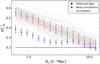 |
Fig. 13. Comparison between the clustering signal in our real survey in blue (same as in Fig. 5) and in the 100 simulated samples. Each sample is drawn from a different light-cone realization. The values of the K-estimator for each of the 100 simulated catalogues is represented in gray. The standard deviation of the 100 K-estimator values and their average values are shown in red. |
We find that the clustering in the simulated samples is much stronger than the clustering in the MUSE-Wide survey. Simulated samples present much larger K-values than in the observed data. The two-parameter PL-fit results in very large uncertainties in r0 (consistent with our observed r0) but also points to lower γ values. From the one-parameter PL-fit (fixed γ = 1.8), we obtain  Mpc and derive a bias factor of
  . These are only ≈1.9σ away from our one-parameter best-fit results. However, from the HOD fit we compute
  and
and ![Mathematical equation: $ \log(M_{\mathrm{DMH}}/[h^{-1}\,M_\odot]) = 12.16 ^{+0.11}_{-0.11} $](/articles/aa/full_html/2021/09/aa41226-21/aa41226-21-eq110.gif) . Considering the MDMH values, this differs by 3.2σ from our observations. We note that since the scope of this paper is not to give an extended comparison to simulations, we have restricted our comparison to one LAE model only, and we obviously cannot draw any general conclusion regarding a potential tension between the predicted and observed clustering of LAEs. Thus, we leave more detailed comparisons to future work. We briefly discuss aspects that may plausibly explain the mismatch below.
. Considering the MDMH values, this differs by 3.2σ from our observations. We note that since the scope of this paper is not to give an extended comparison to simulations, we have restricted our comparison to one LAE model only, and we obviously cannot draw any general conclusion regarding a potential tension between the predicted and observed clustering of LAEs. Thus, we leave more detailed comparisons to future work. We briefly discuss aspects that may plausibly explain the mismatch below.
We first note that the mock light cones show prominent redshift spikes that are not present in the real data (see Fig. 14), a noticeable problem that was also discussed in Diener et al. (2017). The super structures seem to dominate the clustering signal and be responsible for most of the disagreement between our measurements and the simulation. The origin of this discrepancy is unclear and could be due to several reasons that need to be addressed in future simulation work, such as inaccuracies in the Lyα RT modelling, the assumed cosmology, the baryonic physics modelling affecting the halo-galaxy relation, cosmic variance, intrinsic Lyα luminosities, or poorly controlled LAE selection in the mocks.
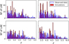 |
Fig. 14. Redshift distribution from four simulated catalogues chosen randomly from the full set of light cones in red. The redshift distribution of the real LAEs from the 68 fields of the MUSE-Wide survey is shown in blue. |
In particular, a potential cause could arise from the fact that Lyα luminosities in GALICS are angle-averaged, whereas the Lyα escape fraction is supposedly highly anisotropic in real galaxies, such that observed Lyα luminosities strongly vary from one sight line to another (Smith et al. 2019). Since the luminosity function of our LAEs is steep, this has the same effect as photometric scattering. Uncertainties in the selection function of GALICS and of observations due to field to field variation are poorly controlled and have a similar effect. This results in the selection of more luminous galaxies at higher redshifts, which can boost the clustering signal.
Moreover, potential deviations on the Lyα luminosity-halo mass relation in GALICS (e.g. star formation not sufficiently quenched in massive halos, such that LLyα = 1042 erg s−1 LAEs might reside in too massive halos) would also enhance the clustering. Besides, a duty cycle (e.g. Ouchi et al. 2010) further powers this mismatch because in GALICS most star forming galaxies emit Lyα. Alternative modelling could lead to Lyα-bright phases that only last a limited period of time, which could plausibly attenuate the strong spikes seen in the redshift distribution.
Since these simulations do not closely reproduce the clustering present in the real data, it is not possible to use them for improving the error estimates on the measurements over the approaches we considered in Appendix C. Nevertheless, simulations can provide information on the individual contribution of the statistical uncertainty and the uncertainty due to cosmic variance. For the statistical uncertainty, we performed 500 K-estimator measurements on the same bootstrap-resampled light-cone (see Sect. 3.1.3 where we apply the same method to our real data). The uncertainty of the cosmic variance can be estimated by computing the standard deviation of the 100 different light-cone realizations. In comparing the individual data points, we find that the uncertainty due to the cosmic variance (red error bars in Fig. 13) is on average ∼35% larger than the error from the statistical approach only (similar to the blue error bars in Fig. 13 but for one light-cone). We have verified that similar results can be found if we resample different light cones. Therefore, our quadratically combined uncertainties (statistical and cosmic variance) in the observed clustering may ultimately be ∼70% higher.
Finally, we used the light cones to check the effects of our special survey geometry. Even if we do not expect a strong effect on the K-estimator since we are measuring a contrast of galaxy pairs in two consecutive shells along LOS separations (see also Appendix A), we compared the clustering of the 100 simulated catalogues in a 68 fields special geometry with the clustering present in the full area of the simulation without any forced geometry (just a simple square of 17 × 17 arcmin2). We find that the signals agree very well.
5.6. The fate of LAEs over cosmic time
Applying an HOD modelling to the K-estimator determines a typical dark matter halo mass of ![Mathematical equation: $ \log (M_{\mathrm{DMH}}/[h^{-1}\,M_\odot]) = 11.34^{+0.23}_{-0.27} $](/articles/aa/full_html/2021/09/aa41226-21/aa41226-21-eq111.gif) for our LAEs. It is expected that these high redshift DMHs significantly grow all the way down to z = 0. We here explore the evolution of those DMHs from ⟨zpair⟩≃3.82 to z = 0 to find the typical descendants of our LAE sample.
for our LAEs. It is expected that these high redshift DMHs significantly grow all the way down to z = 0. We here explore the evolution of those DMHs from ⟨zpair⟩≃3.82 to z = 0 to find the typical descendants of our LAE sample.
Considering the galaxy-conserving evolution model of Fry (1996), which assumes the absence of mergers and that the motion of galaxies are driven by gravity only, the large-scale bias factor evolves as:
 (10)
(10)
where b0 is the bias at z = 0 and D(z) is the linear growth factor (e.g. Hamilton 2001).
Using this model, we infer that the halos of LAEs with a median redshift of the number of pairs ⟨zpair⟩≃3.82 evolve into halos with b0 ≈ 1.4 by z = 0, which translates into typical DMH masses of log(MDMH/[h−1 M⊙]) ∼ 13.5. This is ≈15 times more massive than the Milky Way. Based on Ouchi et al. (2010) calculations, in a more realistic Press-Schechter formalism (e.g. Lacey & Cole 1993), the bias evolution curve is slightly lower, meaning a bias closer to b0 ≈ 1.2 rather than b0 = 1.4.
Similar results are also derived from simulations. The information stored in the DM halo merger trees used in GALICS (Garel et al. 2016) allowed a similar study. They found median descendant halo masses of MDMH/[h−1 M⊙]≈2 × 10¹² for z = 3 LAEs, corresponding to the upper limit estimate of the Milky-Way halo mass. For z = 6 LAEs they found median descendant halo masses of MDMH/[h−1 M⊙]≈5 × 10¹³, corresponding to group or cluster galaxy halos. These assessments are thoroughly in agreement with our estimations and reinforce the notion that our LAEs actually contain a diverse population of objects (as expected, since MUSE-Wide is a Lyα-flux limited survey over a wide z range).
Our work and the various studies presented in the literature cover wide z and Lyα luminosity ranges. If there are indeed clustering dependencies with one or both parameters, this would lead to different typical DMH masses, depending on the details of the sample selection. It is thus necessary to discuss the descendants with respect to different redshift and luminosity progenitors. The combination of clustering measurements of NB-selected LAEs and the galaxy-conserving model considered in this work, leads us to the conclusion that z = 5.7 − 6.6 LAEs will evolve into DMH with bias values of b0 = 1.5 − 2 at z = 0 (Ouchi et al. 2010). This is in agreement with our findings. These higher values, in comparison to those of Gawiser et al. (2007) at z = 3.1, indicate that descendants of LAEs at different redshifts differ. While most LAEs at 4 < z < 7 are probably the large galaxies of today, LAEs at z = 3 are more likely to be the ancestors of Milky Way type galaxies.
Khostovan et al. (2019) considered narrowband-selected LAEs with typical LLyα ∼ 1042 − 43 erg s−1 and intermediate-band-selected LAEs with typical LLyα ∼ 1043 − 43.6 erg s−1 at 2.5 < z < 6. Assuming halo mass accretion models, they found that the former evolved into galaxies residing in halos of typically log(MDMH/[h−1 M⊙]) = 12 − 13 (Milky Way-like) while the later evolved into galaxies residing in halos of log(MDMH/[h−1 M⊙]) > 13 (cluster-like) in the local Universe.
Since our LAEs are in the redshift range of 3.3 < z < 6 and present typical Lyα luminosities in the range 40.9 < log(LLyα/[erg s−1]) < 43.3, the derived descendant masses (log(MDMH/[h−1 M⊙]) ∼ 13.5) are thoroughly in agreement with the cluster-like descendants found by Ouchi et al. (2010) and Khostovan et al. (2019). These results, along with those from literature, reveal that LAEs cover a wide range of present-day descendants, depending on their luminosity and redshift, from Milky Way-type galaxies all the way to clusters of galaxies.
6. Conclusions
In this work, we examine the galaxy clustering properties of a sample of 695 LAEs from the MUSE-Wide survey in the redshift range of 3.3 < z < 6. We applied an optimized version of the K-estimator and supported our results with the traditional two-point correlation function, measuring, for the first time, the spatial clustering as a function of distance in a spectroscopic sample of Lyα-selected galaxies.
Due to the characteristics of the survey (special geometry, large redshift range and limited angular coverage), we focus on the more appropriate clustering method, namely, the K-estimator. We then relied on the radial clustering and quantified the clustering signal following different approaches. We first obtained  Mpc and
  by fitting the clustering signal with a power-law-based correlation function. We derived a bias parameter of
  and compared it to that derived from the second fit approach,
  , by scaling a halo occupation distribution model to the measured signal. The large-scale bias corresponds to typical dark matter halo masses of log
![Mathematical equation: $ (M_{\mathrm{DMH}}/[h^{-1}\,{M}_\odot]) = 11.34^{+0.23}_{-0.27} $](/articles/aa/full_html/2021/09/aa41226-21/aa41226-21-eq117.gif) . In order to support the less known K-estimator method, we also computed the traditional 2pcf, whose results are consistent with those obtained with the K-estimator.
. In order to support the less known K-estimator method, we also computed the traditional 2pcf, whose results are consistent with those obtained with the K-estimator.
The results are also in general agreement with the last available measurements at similar redshifts, with bias factors slightly higher than those in the literature. Nevertheless, most of the previous studies have been carried out in surveys with somewhat different flux limits than that of the MUSE-Wide survey. This could play an important role since we may probe disparate stellar masses. The chosen cosmology and the redshift evolution of these parameters through different epochs also contribute to those slight differences.
We also explore possible clustering dependencies on physical properties. We exclude the possibility of a strong clustering dependence on Lyα equivalent width, UV absolute magnitude, and redshift. However, we see a tentative weak trend when we split the sample at the median Lyα luminosity that is, more luminous LAEs cluster more strongly than less luminous LAEs.
We compare the clustering in the MUSE-Wide survey with the clustering in 100 light cones from a GADGET dark matter only cosmological simulation coupled to the GALICS semi-analytical modelling of LAEs. We find that even though the simulation mimics the flux and luminosity of the LAEs, it is far from successfully reproducing the observed clustering. Simulated data show a stronger clustering than measured in our sample. In order to better imitate the clustering of LAEs, determine the reliable 2pcf scales, compute more realistic uncertainties for our methods, and constrain a physically robust model for LAEs, future simulation studies need to address this challenge.
Assuming galaxy-conserving evolution models, we inferred that our DMHs should evolve into halos of log(MDMH/[h−1 M⊙]) ∼ 13.5 in the local Universe. Since these models assume that the motion of galaxies is driven entirely by gravity, and that mergers do not occur, our evolved DMH masses would be slightly higher in a (more realistic) Press-Schechter formalism. We deduce that the LAEs observed at 3.3 < z < 6 with 40.9 < log(LLyα/[erg s−1]) < 43.3 have mainly evolved into halos hosting galaxies or groups that are ≈15 times more massive than the halo hosting the Milky Way.
A radial extension of the MUSE-Wide survey would benefit the development of LAE clustering studies. Larger areas of the sky would be covered (i.e. larger clustering scales), a larger sample of LAEs would be detected, and the higher S/N would further decrease the uncertainties in the measurements. This will be the case for HETDEX (Hill et al. 2008), which will provide a higher S/N and a much broader coverage of the sky, contributing to improving the understanding of the cosmology behind LAEs.
Acknowledgments
The authors give thanks to the staff at ESO for extensive support during the visitor-mode campaigns at Paranal Observatory. We thank the eScience group at AIP for help with the functionality of the MUSE-Wide data release webpage. M.K. acknowledges support by DLR grant 50OR1904 and DFG grant KR 3338/4-1. L.W. and T.U. acknowledge funding by the Competitive Fund of the Leibniz Association through grants SAW-2013-AIP-4 and SAW-2015-AIP-2. T.M. thanks for financial support by CONACyT Grant Científica Básica #252531 and by UNAM-DGAPA (PASPA and PAPIIT IN111319). T.G. is supported by the ERC Starting Grant 757258 “TRIPLE”. The data were obtained with the European Southern Observatory Very Large Telescope, Paranal, Chile, under Large Program 185.A-0791. This research made use of Astropy, a community-developed core Python package for Astronomy (Astropy Collaboration 2013). We also thank the referee for an useful and constructive report.
References
- Adelberger, K. L., Steidel, C. C., Pettini, M., et al. 2005, ApJ, 619, 697 [NASA ADS] [CrossRef] [Google Scholar]
- Ahumada, R., Prieto, C. A., Almeida, A., et al. 2020, ApJS, 249, 3 [Google Scholar]
- Astropy Collaboration (Robitaille, T. P., et al.) 2013, A&A, 558, A33 [NASA ADS] [CrossRef] [EDP Sciences] [Google Scholar]
- Bacon, R., Accardo, M., Adjali, L., et al. 2010, Proc. SPIE, 7735, 773508 [Google Scholar]
- Bielby, R. M., Tummuangpak, P., Shanks, T., et al. 2001, MNRAS, 456, 4061 [Google Scholar]
- Coil, A. L. 2012, Planets, Stars and Stellar Systems (Dordrecht: Springer), 6 [Google Scholar]
- Coil, A. L., Georgakakis, A., Newman, J. A., et al. 2009, ApJ, 701, 1484 [NASA ADS] [CrossRef] [Google Scholar]
- Colless, M., Dalton, G., Maddox, S., et al. 2012, MNRAS, 328, 1039 [Google Scholar]
- Cowie, L. L., & Hu, E. M. 1998, ApJ, 115, 1319 [Google Scholar]
- Davis, M., & Peebles, P. J. E. 1983, ApJ, 267, 465 [NASA ADS] [CrossRef] [Google Scholar]
- Dayal, P., & Libeskind, N. I. 2012, MNRAS, 419, L9 [NASA ADS] [CrossRef] [Google Scholar]
- Diener, C., Wisotzki, L., Schmidt, K. B., et al. 2017, MNRAS, 471, 3186 [NASA ADS] [CrossRef] [Google Scholar]
- Durkalec, A., Le Fèvre, O., Pollo, A., et al. 2014, A&A, 583, A128 [Google Scholar]
- Durkalec, A., Le Fèvre, O., Pollo, A., et al. 2018, A&A, 612, A42 [NASA ADS] [CrossRef] [EDP Sciences] [Google Scholar]
- Forero-Romero, J. E., Yepes, G., Gottlöber, S., et al. 2011, MNRAS, 415, 3666 [NASA ADS] [CrossRef] [Google Scholar]
- Fry, J. N. 1996, ApJ, 461, L65 [NASA ADS] [CrossRef] [Google Scholar]
- Garel, T., Blaizot, J., Guiderdoni, B., et al. 2012, MNRAS, 422, 310 [NASA ADS] [CrossRef] [Google Scholar]
- Garel, T., Blaizot, J., Guiderdoni, B., et al. 2015, MNRAS, 450, 1279 [Google Scholar]
- Garel, T., Guiderdoni, B., & Blaizot, J. 2016, MNRAS, 455, 3436 [NASA ADS] [CrossRef] [Google Scholar]
- Gawiser, E., Francke, H., Lai, K., et al. 2007, ApJ, 671, 278 [NASA ADS] [CrossRef] [Google Scholar]
- Gurung-López, S., Orsi, A., Bonoli, S., et al. 2018, MNRAS, 486, 1882 [Google Scholar]
- Gurung-López, S., Saito, S., Baugh, C. M., et al. 2021, MNRAS, 500, 603 [Google Scholar]
- Guzzo, L., Scodeggio, M., Garilli, B., et al. 2014, A&A, 566, A108 [NASA ADS] [CrossRef] [EDP Sciences] [Google Scholar]
- Hamilton, A. J. S. 2001, MNRAS, 322, 419 [NASA ADS] [CrossRef] [Google Scholar]
- Hashimoto, T., Verhamme, A., Ouchi, M., et al. 2015, ApJ, 812, 157 [NASA ADS] [CrossRef] [Google Scholar]
- Herenz, E. C., & Wisotzki, L. 2017, A&A, 602, A111 [NASA ADS] [CrossRef] [EDP Sciences] [Google Scholar]
- Herenz, E. C., Urrutia, T., Wisotzki, L., et al. 2017, A&A, 606, A12 [NASA ADS] [CrossRef] [EDP Sciences] [Google Scholar]
- Herenz, E. C., Wisotzki, L., Saust, R., et al. 2019, A&A, 621, A107 [NASA ADS] [CrossRef] [EDP Sciences] [Google Scholar]
- Hill, G. J., MacQueen, P. J., Smith, M. P., et al. 2008, Proc. SPIE, 7014, 701470 [NASA ADS] [CrossRef] [Google Scholar]
- Hinshaw, G., Larson, D., Komatsu, E., et al. 2013, ApJS, 208, 19 [Google Scholar]
- Inami, H., Bacon, R., Brinchmann, J., et al. 2017, A&A, 608, A26 [NASA ADS] [CrossRef] [EDP Sciences] [Google Scholar]
- Jenkins, A., Frenk, C. S., Pearce, F. R., et al. 1998, ApJ, 499, 20 [NASA ADS] [CrossRef] [Google Scholar]
- Kaiser, N. 1987, MNRAS, 227, 1 [Google Scholar]
- Kerutt, J. 2017, Astrophysics Source Code Library [record ascl:1703.011] [Google Scholar]
- Khostovan, A. A., Sobral, D., Mobasher, B., et al. 2019, MNRAS, 489, 555 [CrossRef] [Google Scholar]
- Kron, R. 1980, ApJS, 43, 305 [NASA ADS] [CrossRef] [Google Scholar]
- Krumpe, M., Miyaji, T., & Coil, A. L. 2010, ApJ, 713, 558 [NASA ADS] [CrossRef] [Google Scholar]
- Krumpe, M., Miyaji, T., Coil, A. L., & Aceves, H. 2012, ApJ, 746, 1 [NASA ADS] [CrossRef] [Google Scholar]
- Krumpe, M., Miyaji, T., Husemann, B., et al. 2015, ApJ, 815, 21 [NASA ADS] [CrossRef] [Google Scholar]
- Krumpe, M., Miyaji, T., Coil, A. L., & Aceves, H. 2018, MNRAS, 474, 1773 [NASA ADS] [CrossRef] [Google Scholar]
- Lacey, C., & Cole, S. 1993, MNRAS, 262, 627 [NASA ADS] [CrossRef] [Google Scholar]
- Landy, S. D., & Szalay, A. S. 1993, ApJ, 412, 64 [Google Scholar]
- Le Fèvre, O., Guzzo, L., Meneux, B., et al. 2005, A&A, 439, 877 [NASA ADS] [CrossRef] [EDP Sciences] [Google Scholar]
- Le Fèvre, O., Tasca, L. A. M., & Cassata, P. 2015, A&A, 576, A79 [NASA ADS] [CrossRef] [EDP Sciences] [Google Scholar]
- Li, C., Kaummann, G., Jing, Y., et al. 2006, MNRAS, 368, 21 [NASA ADS] [CrossRef] [Google Scholar]
- Lilly, S. J., Le Fèvre, O., Renzini, A., et al. 2007, ApJS, 172, 70 [NASA ADS] [CrossRef] [Google Scholar]
- Limber, D. N. 1953, ApJ, 117, 134 [NASA ADS] [CrossRef] [Google Scholar]
- Ling, E. N., Frenk, C. S., & Barrow, J. D. 1986, MNRAS, 223, 21P [NASA ADS] [CrossRef] [Google Scholar]
- Maseda, M. V., van der Wel, A., Rix, H.-W., et al. 2018, ApJ, 854, 29 [NASA ADS] [CrossRef] [Google Scholar]
- Miyaji, T., Zamorani, G., Cappelluti, N., et al. 2007, ApJS, 172, 396 [NASA ADS] [CrossRef] [Google Scholar]
- Miyaji, T., Krumpe, M., Coil, A., & Aceves, H. 2011, The X-ray Universe 2011, 108 [Google Scholar]
- Moustakas, L. A., & Somerville, R. S. 2002, ApJ, 577, 1 [NASA ADS] [CrossRef] [Google Scholar]
- Muzahid, S., Schaye, J., Marino, R. A., et al. 2020, MNRAS, 496, 1013 [CrossRef] [Google Scholar]
- Navarro, J. F., Frenk, C. S., & White, S. D. M. 1997, ApJ, 490, 493 [NASA ADS] [CrossRef] [Google Scholar]
- Newman, J. A., Cooper, M. C., Davis, M., et al. 2013, ApJS, 208, 5 [Google Scholar]
- Norberg, P., Baugh, C. M., Hawkins, E., et al. 2002, MNRAS, 332, 827 [NASA ADS] [CrossRef] [Google Scholar]
- Ouchi, M., Shimasaku, K., Furusawa, H., et al. 2003, ApJ, 582, 60 [NASA ADS] [CrossRef] [Google Scholar]
- Ouchi, M., Shimasaku, K., Furusawa, H., et al. 2010, ApJ, 723, 869 [NASA ADS] [CrossRef] [Google Scholar]
- Ouchi, M., Harikane, Y., Shibuya, T., et al. 2017, PASJ, 70, S13 [NASA ADS] [Google Scholar]
- Orsi, A., Lacey, C. G., & Baugh, C. M. 2012, MNRAS, 425, 87 [NASA ADS] [CrossRef] [Google Scholar]
- Peebles, P. J. E. 1980, The Large-Scale Structure of the Universe (Princeton: Princeton University Press) [Google Scholar]
- Rhoads, J. E., Malhotra, S., Dey, A., et al. 2000, ApJ, 545, L85 [NASA ADS] [CrossRef] [Google Scholar]
- Schmidt, B. K., Kerutt, J., Wisotzki, L., et al. 2021, A&A, in press, https://doi.org/10.1051/0004-6361/202140876 [Google Scholar]
- Sheth, R., Mo, H. J., & Tormen, G. 2001, MNRAS, 323, 1 [NASA ADS] [CrossRef] [Google Scholar]
- Shioya, Y., Taniguchi, Y., Sasaki, S. S., et al. 2009, ApJ, 696, 546 [NASA ADS] [CrossRef] [Google Scholar]
- Skrutskie, M. F., Cutri, R. M., Stiening, R., et al. 2006, AJ, 131, 1163 [NASA ADS] [CrossRef] [Google Scholar]
- Smith, A., Ma, X., Bromm, V., et al. 2019, MNRAS, 484, 39 [NASA ADS] [CrossRef] [Google Scholar]
- Sobral, D., Matthee, J., Best, P., et al. 2017, MNRAS, 466, 1242 [NASA ADS] [CrossRef] [Google Scholar]
- Springel, V., White, S. D. M., Jenkins, A., et al. 2005, Nature, 435, 629 [NASA ADS] [CrossRef] [PubMed] [Google Scholar]
- Steidel, C. C., & Hamilton, D. 1992, AJ, 104, 941 [NASA ADS] [CrossRef] [Google Scholar]
- Strauss, M. A., Weinberg, D. H., Lupton, R. H., et al. 2002, AJ, 124, 1810 [NASA ADS] [CrossRef] [Google Scholar]
- Tinker, J. L., Weinberg, D. H., & Zheng, Z. 2005, MNRAS, 368, 85 [Google Scholar]
- Urrutia, T., Wisotzki, L., Kerutt, J., et al. 2019, A&A, 624, A24 [CrossRef] [EDP Sciences] [Google Scholar]
- Van Den Bosch, F. C. 2002, MNRAS, 331, 98 [CrossRef] [Google Scholar]
- Van Den Bosch, F. C., More, S., Cacciato, M., et al. 2013, MNRAS, 430, 725 [NASA ADS] [CrossRef] [Google Scholar]
- Verhamme, A., Garel, T., Ventou, E., et al. 2018, MNRAS, 478, 60 [Google Scholar]
- Yajima, H., Li, Y., & Zhu, Q. 2012, AASMA, 219, 129 [Google Scholar]
- Zehavi, I., Blanton, M. R., Frieman, J. A., et al. 2002, ApJ, 571, 172 [NASA ADS] [CrossRef] [Google Scholar]
- Zehavi, I., Zheng, Z., Weinberg, D., et al. 2011, ApJ, 736, 59 [NASA ADS] [CrossRef] [Google Scholar]
- Zheng, Z., & Weinberg, D. H. 2007, ApJ, 659, 1 [NASA ADS] [CrossRef] [Google Scholar]
- Zheng, Z., Coil, A., & Zehavi, I. 2007, ApJ, 667, 760 [NASA ADS] [CrossRef] [Google Scholar]
Appendix A: Effect of the HUDF parallel fields on the K-estimator
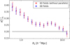 |
Fig. A.1.
|

In this work, we focus on 68 fields of the MUSE-Wide survey, including part of the CANDELS/GOODS-S region and the eight parallel HUDF fields. In order to assess a homogeneous sample, cover a larger area of the sky, and maximize the number of detected galaxies, we include the eight HUDF parallel fields. In this section we explore the possible effects on the clustering measurements of including the parallel fields. We study the clustering in the 68 fields (same as throughout the paper) and that present in the 60 fields (without including the eight parallel HUDF fields). The characteristics of the first sample are described in Sect. 2 while the second sample covers a total of 54.74 arcmin2 and has 581 LAEs.
The K-estimator is then run in both samples and shown in Fig. A.1. We demonstrate the insignificant effect on our main results due to the inclusion or exclusion of the parallel fields. The two curves are indistinguishable within the approximated Poissonian uncertainties  (see Sect. 4.2 in Adelberger et al. 2005) but due to the lower number of LAEs in the 60 fields the uncertainties are somewhat larger (8%) than those of the 68 fields.
The minimal effect on the clustering signal, the larger area of the sky covered, which makes it more representative in terms of cosmic variance, and the larger number of LAEs in the sample, which reduce the uncertainties, lead us to include the eight parallel HUDF fields in our analysis of the main sample.
Appendix B: Effect of Lyα derived redshifts on the K-estimator
Inferring the redshift of galaxies from their Lyα lines introduces an offset (i.e. a few hundreds of km/s) with respect to their systemic redshift (Hashimoto et al. 2015). This offset translates into small uncertainties in the derived positions of the galaxies (i.e. ∼3 Mpc) that would affect the clustering measurements when scrutinized through traditional methods (see e.g. Gurung-López et al. 2021). The K-estimator compares galaxy pair counts in two consecutive shells along LOS separations. Thus, the offset introduced in the separations affects both shells equally, being simultaneously compensated. However, since we are working with much larger scales than ∼3 Mpc, even from a theoretical point of view, the K-estimator is not expected to be sensitive to these redshift offsets.
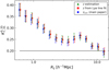 |
Fig. B.1.
|

We prove this in Fig. B.1, considering the same sample of LAEs, but obtaining the redshift of the galaxies in different manners. We first use the redshift estimates from QtClassify (see Sect. 2) and then we use more precise redshifts obtained by fitting asymmetric Gaussian profiles to the Lyα emission lines. Finally, from those precise redshifts we correct the redshift following Verhamme et al. (2018) as described in Sect. 2.2. We run the K-estimator for these three samples, which only differ by their source redshift estimates. In Fig. B.1, we show the minimal impact of the redshift uncertainties in our results, showing that the three different redshift samples provide negligible variations in the K-estimator values.
The K-estimator on the sample with redshift estimations provides large-scale bias factors of  from PL fits, while using the sample with the corrected redshifts (main paper)
  .
.
Appendix C: Error estimates in the K-estimator
When computing the clustering signal with the K-estimator, we have to recognize that the individual data points are correlated. Various galaxy pairs can be part of more than one Rij bin and the same galaxy may be counted in more than one galaxy pair. The extent of how bin i correlates with bin j is usually expressed with the covariance matrix. However, the small area covered by our survey does not allow us to calculate a covariance matrix. Therefore, we investigated several error approaches for our K-estimator measurements.
We applied the bootstrapping technique described in Ling et al. (1986), which creates pseudo-data sets by sampling N sources with replacement from the real sample of N galaxies. In other words, we randomly draw objects from the real sample, allowing multiple selections of the same object, to generate a pseudo-sample with the same number of objects N as the real sample. We repeat the process 500 times, obtaining a large set of pseudo-samples, which vary moderately from the original data. We compute the K-estimator in the 500 pseudo-samples, Nboots = 500. The scatter from all the measurements is adapted for our uncertainty estimations.
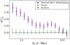 |
Fig. C.1.
|

We also considered a second technique, in which we generate random samples. Ideally, 500 different realizations from cosmological simulations should be applied but we showed in Sect. 5.5 that the simulated data cannot directly be compared to our clustering measurements.
Therefore, we use the selection and luminosity functions of the survey (Herenz et al. 2019) to obtain the real z-distribution of our LAEs (see Sect. 2 and red curve in Fig. 2). Randomly clustered samples with the same number of objects as the real sample are created from the real redshift distribution. Each new galaxy is located at a random position within the MUSE-Wide survey footprint, with a specific redshift provided by the combination of LF and SF. Following this procedure, we generate 500 different random samples and compute  in each of the samples. For each bin, the uncertainty has been obtained as the standard deviation from the resulting
  of the different 500 random samples.
We show the two main uncertainty approaches for the K-estimator in Fig. C.1. We also include the approximated Poisson errors  calculated by the error propagation of Eq. 1.
While the random errors are 20% smaller than Poisson errors, we find that the uncertainties from bootstrapping are moderately larger (∼35%) than the Poissonian ones. In order to remain conservative (and even if all uncertainties are comparable), we decided to compute the error bars in our K-estimator analyses following the classical bootstrapping approach. Hence, uncertainties due to cosmic variance are not represented yet in our error estimates of the real data. In other words, repeating the same LAE clustering studies in different regions of the sky can lead to clustering signals outside our expected uncertainty range. The cosmic variance contribution to the total error budget was explored in Sect. 5.5. Including this contribution results in ∼70% larger uncertainties. However, this additional uncertainty does not impact our results when comparing the subsamples because they are obtained in the same sky field.
Appendix D: Two-point correlation function analysis
D.1. 2pcf method
Overall, 2pcf is the most commonly used statistical approach to explore the clustering in a sample of objects. Traditionally, those samples cover a broad spatial coverage that accounts for cosmic variance and allows the computation of a covariance matrix to estimate clustering uncertainties. With the MUSE-Wide survey, we are facing the opposite scenario: small spatial coverage and a wide redshift range.
In reconstructing the 2pcf, we follow standard recipes (Landy & Szalay 1993). To recall, ξ(r) quantifies the excess probability P over a random Poisson distribution of finding a pair of galaxies separated by a distance r (Peebles 1980)
![Mathematical equation: $$ \begin{aligned} dP = n[1 + \xi (r)]\mathrm{d}V, \end{aligned} $$](/articles/aa/full_html/2021/09/aa41226-21/aa41226-21-eq128.gif) (D.1)
(D.1)
where dV is the infinitesimal volume occupied by the pair and n is the average number density of galaxies.
Galaxy distances along the light of sight (LOS) cannot be measured directly. Instead the redshift information of the galaxies is used, which is affected by their peculiar velocities. In order to eliminate this effect, the so-called redshift space distortions (RSD), we compute the correlation function in a 2D grid. We measure the separation of pairs in the perpendicular distance to the LOS direction, rp, and parallel to the LOS direction, π. We then count pairs of LAEs within given separations and compare them to those in a random sample of galaxies by means of the Landy-Szalay estimator (Landy & Szalay 1993)
 (D.2)
(D.2)
where DD, RR and DR are the normalized data-data, random-random and data-random pairs. In other words, expressing the actual number of pairs as npair, DD(rp, π), npair, DR(rp, π) and npair, RR(rp, π):
![Mathematical equation: $$ \begin{aligned}&DD = n_{\mathrm{pair},DD}(r_p, \pi )/[N_D(N_D-1)]\nonumber\\&DR = \frac{1}{2} n_{\mathrm{pair},DR}(r_p, \pi )/(N_D N_D)\nonumber\\&RR = n_{\mathrm{pair},RR}(r_p, \pi )/[N_R(N_R-1)]. \end{aligned} $$](/articles/aa/full_html/2021/09/aa41226-21/aa41226-21-eq130.gif) (D.3)
(D.3)
ND and NR are the total number of galaxies in the real and random sample, respectively.
We then calculate the projected correlation function ω(rp) by integrating ξ(rp, π) along the π-direction (Davis & Peebles 1983)
 (D.4)
(D.4)
where ωp is the projected 2pcf and πmax is the maximum allowed LOS distance between pairs of galaxies to be considered as a pair. Also, πmax is chosen such that it accounts for most correlated pairs and the amplitude of ωp(rp) is able to converge. Very large values would mainly increase the noise since there are not many correlated pairs at large LOS distances. In contrast, very low values would not include most correlated pairs and would effectively underestimate ωp(rp).
 |
Fig. D.1. Best PL and HOD fits to the projected 2pcf ωp(rp) for πmax = 60 h−1 Mpc. The dashed green curve shows the PL-fit while the dotted red curve represents the HOD fit. The error bars are determined from the random approach explained in Appendix D.2. |
We compute π within 10−300 h−1 Mpc in steps of 10 h−1 Mpc and rp in the range of 0.375 < rp/h−1 Mpc < 13.155 in 9 logarithmic bins. We then calculate the projected correlation function ωp(rp) for each π value and fit the analytical solution:
 (D.5)
(D.5)
where Γ(x) is the Gamma function. The fittings are performed in the range 0.584 < rp/h−1Mpc < 13.155 (two-halo term only) for each of the ωp(rp) curves.
We measure the correlation length of the curves using Eq. D.5 with a fixed slope of γ = 1.8. In order to be conservative, we use πmax = 60 h−1 Mpc. Similar πmax values are obtained with the simulation described in Sect. 5.5. Literature πmax values in similar LAE clustering studies used less conservative values (15−20 h−1 Mpc; Durkalec et al. 2014, 2018).
Besides the πmax determination, the measurement of the 2pcf also demands the modelling of a random sample of galaxies with the same geometry, selection effects and observational conditions as the real sample. Hence, we constructed a random sample from the real z-distribution of the sample (red curve in Fig. 2) obtained from the SF and the LF of the MUSE-Wide survey (Herenz et al. 2019). The number of random objects is chosen to be 100 times the number of galaxies in the real sample. This makes the variance of DR and RR in Eq. D.2 negligible. We verified that increasing the number of random galaxies or using different random samples have an insignificant effect on our estimates. Each random galaxy is then located at a random position of the sky within the MUSE-Wide survey footprint, with a redshift taken from the real z-distribution. Given that our πmax is much smaller than the radial comoving distance corresponding to our sample redshift range, over which the random sample is constructed, the effects for the integral constraint are negligible for our ωp(rp).
D.2. Error estimates
The bootstrapping approach applied in the K-estimator method allows for replacement and galaxy repetitions. This produces an overlap of galaxies, which introduces an unrealistic clustering excess in the 2pcf. While this does not affect the K-estimator because it measures a contrast of galaxy pairs between two LOS regions and overlaps of galaxies cancel out in both areas, the 2pcf is severely affected. We therefore do not consider the bootstrapping approach as a possible error determination technique for the 2pcf.
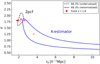 |
Fig. D.2. Analogous to Fig. 6, here showing the contours from the 2pcf method in black-gray. For a direct comparison to the K-estimator, its contours have been represented in blue, as well as the r0 computed from both methods when fixing the slope of the PL to the standard value, shown with dots. Please note that we consider the contours of the 2pcf to be likely underestimated (see text for further details). |
We consider an alternative approach by generating random samples. Analogous to the error estimates in the K-estimator, 100 different light cones from cosmological simulations should be used instead; however, it was shown in Sect. 5.5 that the simulated data should not be directly compared to our measurements. Thus, we created random samples from the real redshift distribution of our LAEs. The random samples have the same number of objects as the MUSE-Wide survey. The real redshift distribution is calculated from the luminosity and the selection function of the sample (Herenz et al. 2019) as described in Sect. 2. We denote the newly created random sample by R′ to distinguish from the random sample R in Eq. D.2. The 2pcf in the random samples is calculated by replacing D by R′ in Eq. D.2 for 100 different newly generated random samples R′ (i.e. Nran = 100). The scatter of the 100 runs is used as our uncertainty estimation.
This approach is compared to Poissonian errors calculated by error propagation in Eq. D.2,  . We find that the Poissonian uncertainties underestimate the true clustering errors compared to the random-sample approach (uncertainties from the random error approach are ∼65% larger than Poisson errors). However, even the uncertainties from the random error approach should be understood only as a first guess. The combination of the 2pcf and the special design of our MUSE-Wide survey leave this as the only option to estimate the extent of the uncertainties on the 2pcf.
D.3. Results
We present the projected correlation function ωp(rp) for πmax = 60 h−1 Mpc over the range of 0.375 < rp/h−1 Mpc < 13.155 in Fig. D.1. The error bars in ωp(rp) have been computed following the random-sample approach described in Appendix D.2.
Despite the small area covered by the MUSE-Wide survey, the ωp(rp) curve shows a clear clustering signal. The large number of galaxies in the MUSE-Wide survey allow us to fit the clustering signal with a PL-based correlation function, where both correlation length and slope are constrained simultaneously. Thus, we set r0 and γ as the free parameters to be determined from the fit.
Best-fit clustering parameters from 2pcf measurements.
We then use Eq. D.5 to fit ωp(rp) in the two-halo term, 0.584 < rp/h−1 Mpc < 13.155. We also use this rp range to fit the curve with the HOD model described in Sect. 3.4, same as for the K-estimator. The measured best-fit parameters are listed in Table D.1 and shown in Fig. D.1. The probability contours from the r0-γ grid of the PL-fit are shown in Fig. D.2, along with those from the K-estimator to allow a direct comparison (see Appendix D.4 for a discussion of the different clustering methods and results).
With the PL-fit, we find  Mpc with a correlation slope γ = 1.85 ± 0.25. These parameters correspond to
  . These results are in agreement with the derived correlation lengths from the one-bin fit (fixed γ = 1.8) and from the PL-fit (free r0 and γ) to the K-estimator (contours in Fig. D.2). However, for the 2pcf case, γ is much closer to the canonical value than the K-estimator. When considering HOD fits, we obtain b = 2.05 ± 0.14, somewhat lower (1.3σ) than the b = 2.80 ± 0.38 obtained with the K-estimator. The differences in the derived linear bias factors from PL and HOD fits are discussed in detail in Sect. 5.3.
In order to better constrain the correlation parameters, we fix the correlation slope and determine only the correlation length. Following this procedure (and in an effort to remain consistent with the literature), we fix the slope to γ = 1.8 and derive from the one-parameter fit r0 = 1.85 ± 0.15 h−1 Mpc. This value agrees at a one sigma level with the one derived from the K-estimator ( Mpc; fixed γ = 1.8).
D.4. K-estimator vs 2pcf
The various clustering methods studied in this paper allow us to compare not only their respective results but also their success as methods themselves in these sort of surveys. While the 2pcf is well known, the K-estimator is still relatively unexplored. However, for galaxy surveys that cover small areas of the sky, but span wide redshift ranges the K-estimator seems to be a more suitable clustering method than the commonly used 2pcf. Both methods have important similarities but also present critical differences. First of all, the concept of measuring clustering itself differs. While the 2pcf measures the spatial clustering by comparing pairs of galaxies to those in random samples, the K-estimator compares the contrast of galaxy pairs in two consecutive shells along LOS distances, without introducing any random sample and focusing on redshift clustering rather than on spatial clustering. Secondly, choosing the most suitable K-estimator or the upper integration limit πmax in the 2pcf share some concepts. The πmax value where the 2pcf saturates collects the maximum number of galaxy pairs and tries to discard noise from distant uncorrelated pairs. The a2 and a3 values of the K-estimator boost the clustering signal by finding the two shells along LOS separations where the highest contrast of galaxy pairs is encountered. Therefore, πmax just represents an upper integration limit in LOS distances and a2 and a3 are the length of the shells with the highest difference in pair counts. Typically, a3 should be below the upper integration limit πmax. Finally, both methods quantify the clustering of a sample of galaxies by counting galaxy pairs in 3D space.
Although the two methods present a clustering signal over equal transverse distances, Rij and rp, and the ai values are within the πmax limit, the fitting parameters are somewhat distinct. This was expected because, first, the 2pcf in this type of surveys has issues. Its performance is affected by the small spatial coverage of the data and the survey geometry. We do not see a clear saturation point of the ω(rp) curves for the different πmax values and, in addition, error estimations, such as the jackknife method, fail. Hence, we believe that we are exploring the limit of the method. Secondly, the fits for both methods are carried out in different ways (see Sect. 3.1 and Appendix D.3). While we fit ωp(rp) with its analytical solution (Eq. D.5), the K-estimator is either compared to the expectation value of  (Eq. 2) through the one-fit approach or fitted with a PL with the PL-fit approach. If we allow r0 and γ to freely vary in the fit for both methods, the correlation lengths, bias factors and DMH masses obtained from the K-estimator and the 2pcf are
  h−1 Mpc,
 , log
, log![Mathematical equation: $ (M_{\mathrm{DMH}}/[h^{-1}\,{M}_\odot])=11.34^{+0.23}_{-0.27} $](/articles/aa/full_html/2021/09/aa41226-21/aa41226-21-eq146.gif) and
and  h−1 Mpc, γ = 1.85 ± 0.25,
  and log
![Mathematical equation: $ (M_{\mathrm{DMH}}/[h^{-1}\,{M}_\odot])=10.51^{+0.16}_{-0.17} $](/articles/aa/full_html/2021/09/aa41226-21/aa41226-21-eq149.gif) , respectively. Even if the HOD fits from the K-estimator are higher (1.3σ) than those computed with the 2pcf, the 68.3% confidence intervals of the PL-fits agree.
, respectively. Even if the HOD fits from the K-estimator are higher (1.3σ) than those computed with the 2pcf, the 68.3% confidence intervals of the PL-fits agree.
A noteworthy addition to our discussion is the uncertainty dissimilarities between the methods, where the difference in the probability contour sizes of Fig. D.2 come from. It is important to notice that the uncertainties in the K-estimator were obtained through the bootstrapping approach. However, bootstrapping causes overlaps of galaxies to which the K-estimator is insensitive, but in the 2pcf case, this causes a significant boost in the clustering signal. Thus, we have to consider the random sample approach as the only way to give some educated guess on the 2pcf uncertainties, even if it most likely still underestimates the real uncertainties. Therefore, the 2pcf contour shown in Fig. D.2 is also most likely underestimated.
For the 2pcf we had to apply the standard (uncorrelated) χ2 analysis with likely underestimated uncertainties, while for the K-estimator we were able to renormalize the χ2 analysis and used conservative uncertainty estimates as described in Sect. 3.1.3. Despite these fundamental differences the clustering results derived from both methods still agree within their combined 2σ uncertainties.
The K-estimator is a more suitable clustering statistic than the 2pcf in these kind of surveys for the following reasons: (i) The K-estimator exploits the large redshift coverage rather than the spatial extent (more than 1000 h−1 Mpc along the LOS direction vs only 20 h−1 Mpc over transverse separations); (ii) it does not require a random sample so integral constraint issues do not take place; (iii) we can use bootstrapping uncertainties when the jackknife technique is not an option; and (iv) with the K-estimator we provide a straightforward recipe to obtain rough a2 and a3 values (unlike πmax in the 2pcf).
Appendix E: Effect of redshift space distortions on our measurements
Both PL and HOD fit approaches show a high performance on the K-estimator. Nevertheless, none of them account for the redshift space distortions present in the observations of the high-redshift Universe. Galaxy structures are observed to be ‘falling into’ large-scale overdensities, which varies the projected velocity along the LOS direction from that linked to its cosmological redshift. As explained in Sect. 3.4, we include the effects of the redshift distortion in the HOD model using the linear theory to the two-halo term only. Therefore, the large-scale streaming motion towards overdense regions (i.e. Kaiser infall, Kaiser 1987) is corrected in the linear regime.
In order to account for these effects, we implement the HOD correlation function in redshift space, ξ(s), accounting thus for RSD. We represent the HOD fit to the K-estimator both from the spatial space, ξ(r), (same as in Sect. 4) and the redshift space, ξ(s), in Fig. E.1.
The HOD fit from the redshift space correlation function (i.e. with RSD) is slightly higher than that from the real space correlation function (i.e. without RSD) at small separations (Rij < 1 h−1 Mpc), showing the minimal RSD effect on the K-estimator. This small rise translates into an increase in the derived bias factor, from  to
to  , indistinguishable within the 1σ error bars.
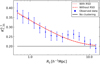 |
Fig. E.1. Best HOD fits to the K-estimator from ξ(r) (same as the thick curve in Fig. 7) and ξ(s). The dotted red curve represents the HOD that takes into account the effect of the RSD, while the dashed red curve shows the HOD fit without RSD. The black line represents an unclustered sample of galaxies. |
All Tables
Clustering parameters from the different fit approaches to the K-estimator in our full sample.
All Figures
|
Fig. 1. Spatial distribution of 695 LAEs covering part of the CANDELS/GOODS-S region and the HUDF parallel fields on the left. The individual LAEs span a total of 68 fields from the MUSE-Wide survey and are color-coded by their Lyα spectroscopic redshift, 3.3 < z < 6. The 5 h−1 Mpc bar for the mean redshift of the sample |
| In the text | |
|
Fig. 2. KDE-filtered redshift distribution of the 695 LAEs of our sample, taken from 68 fields of the MUSE-Wide survey. The sample spans a redshift range of 3.3 < z < 6. The kernel is chosen to be a Gaussian with standard deviation σz = 0.005. The expected z-distribution of an unclustered population following the Lyα luminosity function of Herenz et al. (2019) and the selection function of the MUSE-Wide survey is overplotted in red. |
| In the text | |
|
Fig. 3. Illustration of the K-estimator. We show three nested cylinders representing three bins of transverse separations. The number of galaxy pairs inside each blue cylindrical shell from a1 = 0 to ±a2 is N0, a2, the number of pairs in each red cylindrical shell between a3 − a2 and −a2 − ( − a3) is Na2, a3. The K-estimator for each shell is then the ratio of pair counts between the inner (blue) segment to the total (blue plus red) segment. For illustration purposes we depict linear Rij bins, although in practice we use a logarithmic binning scheme. |
| In the text | |
|
Fig. 4. Results of our grid study to optimize the K-estimator. Left: S/N obtained for each evaluated combination of (a2, a3), displayed as a color map. The green area indicates the ‘forbidden’ range where a3 < a2. The contours trace S/N increments of 2, slightly smoothed for display purposes. Right: same parameters but for the correlation length r0, except that the contours again follow the values of the S/N. The blue-red colored circles represent grid points with a3 = 2a2 for which the blue-red cylinders in Fig. 3 are equally long. The blue cross indicated our adopted parameter combination for the clustering analysis, as it provides the highest S/N and reaches saturation at r0. |
| In the text | |
|
Fig. 5. Measured values of the K-estimator as a function of transverse distance (points with error bars) compared to the expected behaviour for a population strictly following a power-law correlation function. Left: five curves represent different power-law indices as given in the legend, for a fixed value of r0 = 3.6 h−1 Mpc. Right: same details for five different correlation lengths at fixed γ = 1.3. The central (thick solid) curves always indicate the minimum χ2 best-fit values. The horizontal straight line shows the no-clustering expectation value of K. The error bars are calculated with the bootstrapping technique described in Sect. 3.1.3. |
| In the text | |
|
Fig. 6. Simultaneous fit to r0 and slope γ. The black (dark grey) contour represents the 68.3% (95.5%) confidence. The red cross stands for the lowest χ2 value at (r0 = 3.65, γ = 1.25). The points show the 500 best-fit values from the 500 bootstrapped samples. The blue rectangle indicates the 16% and 84% percentiles from the marginalized single-parameter posterior distributions of the bootstrapped samples. The green (red) error bar represents the correlation length from the one-parameter PL (single-bin) fit with fixed γ = 1.8. For a better visualization, we show a zoom onto the region containing these fits. |
| In the text | |
|
Fig. 7. Dependence of the HOD fits to the K-estimator on the large-scale bias factor. The dotted, solid, and dashed red curves show three different bias factors b = 2.3, 2.8, 3.3, respectively. The thicker solid red curve shows the b that provides the lowest χ2 value. The K values and their respective error bars are the same as in Fig. 5. |
| In the text | |
|
Fig. 8. Measured values of the K-estimator of our sample of 68 MUSE-Wide fields (blue filled circles) compared to the subset of 24 fields considered in Diener et al. (2017, D17; open red circles). The error bars are again calculated with the bootstrapping technique described in Sect. 3.1.3. The blue dotted curve represents our two-parameter best PL-fit. The red dotted curve uses the best single-bin fit results of D17 ( |
| In the text | |
|
Fig. 9. Comparison of the derived correlation lengths to the literature. The r0 values calculated in this study are represented with purple stars. Green symbols correspond to studies of samples based on Lyα selected galaxies. The samples from Durkalec et al. (2014) at z ∼ 2.5 and z ∼ 3.5 (dark and light yellow) are based on continuum-selected high-z galaxies. The horizontal colored bars indicate the redshift ranges of the corresponding studies (spectroscopic surveys). The redshift range of the z-subsamples of this paper are not plotted for a better visibility. Values for r0 are plotted at the median redshift of the samples. The r0 from Ouchi et al. (2003) and Bielby et al. (2001) have been shifted by +0.1 along the x-axis for visual purposes. Our one-parameter PL-fit with fixed γ = 1.8 by +0.2. The upper limit of the r0 from Shioya et al. (2009) corresponds to r0 = 10.1 Mpc. |
| In the text | |
|
Fig. 10. Best PL and HOD fits to the K-estimator. The dashed green curve shows the PL-fit (same as the solid curves in Fig. 5) while the dotted red curve represents the HOD fit (same as the thick curve in Fig. 7). The measurements of |
| In the text | |
|
Fig. 11. Comparison between the bias parameters derived from the PL and HOD fits listed in Tables 2 and 3. We highlight the bias factor from the full sample of LAEs with a red square. The dotted blue line shows a 1:1 correspondence. |
| In the text | |
|
Fig. 12. Clustering dependencies on object properties. Top left: clustering variation in two different redshift subsamples. The blue dots show the clustering in the lower redshift bin while the red points show the higher redshift subsample. The dotted curves represent the best HOD fits. Top right: same details but for two different Lyα luminosity subsamples. Bottom left: same details but for EWLyα. Bottom right: same details but for UV absolute magnitude. The black line represents the K expectation value for an unclustered sample of galaxies and the 1σ error bars are determined from the bootstrapping approach explained in Sect. 3.1.3. |
| In the text | |
|
Fig. 13. Comparison between the clustering signal in our real survey in blue (same as in Fig. 5) and in the 100 simulated samples. Each sample is drawn from a different light-cone realization. The values of the K-estimator for each of the 100 simulated catalogues is represented in gray. The standard deviation of the 100 K-estimator values and their average values are shown in red. |
| In the text | |
|
Fig. 14. Redshift distribution from four simulated catalogues chosen randomly from the full set of light cones in red. The redshift distribution of the real LAEs from the 68 fields of the MUSE-Wide survey is shown in blue. |
| In the text | |
|
Fig. A.1.
|
| In the text | |
|
Fig. B.1.
|
| In the text | |
|
Fig. C.1.
|
| In the text | |
|
Fig. D.1. Best PL and HOD fits to the projected 2pcf ωp(rp) for πmax = 60 h−1 Mpc. The dashed green curve shows the PL-fit while the dotted red curve represents the HOD fit. The error bars are determined from the random approach explained in Appendix D.2. |
| In the text | |
|
Fig. D.2. Analogous to Fig. 6, here showing the contours from the 2pcf method in black-gray. For a direct comparison to the K-estimator, its contours have been represented in blue, as well as the r0 computed from both methods when fixing the slope of the PL to the standard value, shown with dots. Please note that we consider the contours of the 2pcf to be likely underestimated (see text for further details). |
| In the text | |
|
Fig. E.1. Best HOD fits to the K-estimator from ξ(r) (same as the thick curve in Fig. 7) and ξ(s). The dotted red curve represents the HOD that takes into account the effect of the RSD, while the dashed red curve shows the HOD fit without RSD. The black line represents an unclustered sample of galaxies. |
| In the text | |
Current usage metrics show cumulative count of Article Views (full-text article views including HTML views, PDF and ePub downloads, according to the available data) and Abstracts Views on Vision4Press platform.
Data correspond to usage on the plateform after 2015. The current usage metrics is available 48-96 hours after online publication and is updated daily on week days.
Initial download of the metrics may take a while.