| Issue |
A&A
Volume 653, September 2021
|
|
|---|---|---|
| Article Number | A163 | |
| Number of page(s) | 20 | |
| Section | Cosmology (including clusters of galaxies) | |
| DOI | https://doi.org/10.1051/0004-6361/202140657 | |
| Published online | 28 September 2021 | |
X-ray analysis of the Planck-detected triplet-cluster system PLCK G334.8-38
1
Université Paris-Saclay, CNRS, Institut d’astrophysique spatiale (IAS), 91405 Orsay, France
e-mail: alex@kolodzig.eu
2
IRAP, Université de Toulouse, CNRS, CNES, UPS, Toulouse, France
Received:
25
February
2021
Accepted:
27
May
2021
We conducted an X-ray analysis of one of the two Planck-detected triplet-cluster systems, PLCK G334.8-38.0, with a ∼100 ks deep XMM-Newton data. We find that the system has a redshift of z = 0.37 ± 0.01 but the precision of the X-ray spectroscopy for two members is too low to rule out a projected triplet system, demanding optical spectroscopy for further investigation. In projection, the system looks almost like an equilateral triangle with an edge length of ∼2.0 Mpc, but masses are very unevenly distributed (M500 ∼ [2.5, 0.7, 0.3]×1014 M⊙ from bright to faint). The brightest member appears to be a relaxed cool-core cluster and is more than twice as massive as both other members combined. The second brightest member appears to be a disturbed non-cool-core cluster and the third member was too faint to make any classification. None of the clusters have an overlapping R500 region and no signs of cluster interaction were found; however, the XMM-Newton data alone are probably not sensitive enough to detect such signs, and a joint analysis of X-ray and the thermal Sunyaev-Zeldovich effect is needed for further investigation, which may also reveal the presence of the warm-hot intergalactic medium within the system. The comparison with the other Planck-detected triplet-cluster-system (PLCK G214.6+36.9) shows that they have rather different configurations, suggesting rather different merger scenarios, under the assumption that they are both not simply projected triplet systems.
Key words: large-scale structure of Universe / X-rays: galaxies: clusters / galaxies: clusters: intracluster medium / galaxies: clusters: general / galaxies: groups: general / X-rays: diffuse background
© A. Kolodzig et al. 2021
 Open Access article, published by EDP Sciences, under the terms of the Creative Commons Attribution License (https://creativecommons.org/licenses/by/4.0), which permits unrestricted use, distribution, and reproduction in any medium, provided the original work is properly cited.
1. Introduction
In the standard paradigm, gravitation drives structure formation in a hierarchical process, and makes dark matter the “scaffolding” of the cosmic web. At first order, ordinary matter follows the dark matter distribution. This has long been demonstrated by theory and numerical simulations of structure formation. However, the role of baryons is much more complex in the process and the details of the physical processes governing this component remain to be understood. In the local Universe, it is expected that the vast majority of baryons (≳80%) have been heated under the action of gravity to temperatures above 105 K, and thus have not condensed into stars (e.g., Cen & Ostriker 1999; Roncarelli et al. 2012; Kravtsov & Borgani 2012; Dolag et al. 2016; Martizzi et al. 2019). This makes studying the “hot” Universe a crucial step towards understanding the formation and evolution of cosmic structures.
Important endpoints of structure formation processes are clusters of galaxies, reaching total masses above 1014 M⊙. Most of their baryonic matter is in the form of a hot (T ≳ 107 K), tenuous plasma, the intracluster medium (ICM; e.g., Sarazin 1988), representing 80 − 90% of the baryonic mass of a cluster of galaxies (e.g., Giodini et al. 2009). However, within the local Universe the ICM only accounts for a small fraction of baryons (∼4%); the majority (∼50%) are expected to reside in the cosmic web in the form of a warm-hot intergalactic medium (WHIM), a cooler and, on average, less dense plasma (T ∼ 105 − 107 K, ne ≲ 104 cm−3) than the ICM (e.g., Cen & Ostriker 2006; Cautun et al. 2014; Martizzi et al. 2019). By understanding the physical state of the hot, diffuse gas and how it gets accreted, heated, and virialized onto clusters of galaxies in order to be transformed from a WHIM state to an ICM state, we can also better understand its role in structure formation.
Ideal places to study such structure formation processes are multi-cluster systems, also called superclusters (SCs). These are the most massive structures of the cosmic web and represent the largest agglomeration of galaxies (of the order of 10 − 100 Mpc h−1), containing thousands of them and a few to dozens of groups and clusters of galaxies (e.g., Einasto et al. 1980; Oort 1983). SCs are already decoupled from the Hubble flow but are not yet virialized and most of them will eventually collapse under the effect of gravity. This makes present-day SCs the largest bound but not yet fully evolved objects in the local Universe, and therefore they can also be seen as “island universes” (e.g., Araya-Melo et al. 2009).
Our current best knowledge of hot gas from SCs comes from targeted observations of nearby, X-ray-bright multiple-cluster systems. These range from simple merging cluster pairs, such as the A399–A401 pair (Ulmer et al. 1979) with its well-studied inter-cluster filament (e.g., Akamatsu et al. 2017; Bonjean et al. 2018; Govoni et al. 2019), to very complex SCs, such as Shapley (Shapley 1930), the richest known SC in terms of X-ray emitting clusters (e.g., Raychaudhury et al. 1991; de Filippis et al. 2005). Studies of those SCs have shown that the hot gas between cluster members of a SC, also known as intra-SC medium (ISCM), is accreted mainly along filaments and gets heated to ICM-like temperatures via shocks and adiabatic compression at the cluster outskirts (e.g., Tozzi et al. 2000; Zhang et al. 2020; Power et al. 2020). Hereby, the interaction and merging of clusters serves as an important catalyst of these accretion and heating processes and gives rise to other heating processes caused by the creation of additional turbulent gas motions (e.g., Sarazin et al. 2002; Shi et al. 2020). This means that the most important gas physics are happening in the outskirts of clusters, beyond their viral radius (e.g., Ryu et al. 2003; Molnar et al. 2009; Nelson et al. 2014; Simionescu et al. 2021).
In this respect, it is important to not just capture the emission of the ICM but also of the ISCM when studying the hot gas of an SC. The hot gas within SCs is visible in the X-rays (through thermal bremsstrahlung and line emission), and at millimeter wavelengths through the thermal Sunyaev-Zeldovich effect (tSZ). However, as it is cooler and less dense, detecting and studying the ISCM is much more challenging than for the ICM (e.g., Werner et al. 2008). One way of tackling this challenge is via stacking analysis. The stacking analysis by Tanimura et al. (2019) using tSZ data from Planck for galaxy-detected SCs revealed that the ISCM accounts for a significant fraction of WHIM (≳10%), which further emphasises SCs as suitable structures with which to study the role of hot bayrons in structure formation. Another promising avenue can be found in joint analyses with X-rays and tSZ of specific SCs, because X-rays are more sensitive to cluster cores, while the tSZ effect is more sensitive to cluster outskirts. The combination of both observables allows us to constrain the distribution of several important physical parameters of the hot baryons over a large physical range (e.g., Eckert et al. 2017; Kéruzoré et al. 2020).
Serendipitously, a cluster-candidate search with Planck data revealed two triplet-cluster systems with favorable system configurations for the joint analysis of a SC of this type. Both are located at redshifts where they are still sufficiently X-ray-bright and they are also sufficiently small such that we can observe the entire system within one field-of-view (FOV) of the X-ray observatory XMM-Newton, which is very well suited to detecting emission from diffuse, hot gas. The search was conducted with the data from the first Planck sky scan (Planck Collaboration VIII 2011) and was followed up with an XMM-Newton observation campaign (Planck Collaboration IX 2011, hereafter PLIX2011). For one of the SCs (PLCK G214.6+36.9), located at z ≈ 0.45, a joint X-ray–tSZ analysis study was conducted (Planck Collaboration Int. VI 2013). The other triplet-cluster system discovered in Planck data, PLCK G334.8-38.0, is the focus of the present paper. In Fig. 1, we show its X-ray and tSZ emission and mark its three cluster members with the letters A, B, and C, which are ordered according to the X-ray surface brightness (hereafter XSB) from bright to faint.
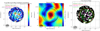 |
Fig. 1. X-ray and tSZ emission of the triplet-cluster system PLCK G334.8-38.0. Left: XMM-Newton background-subtracted, detector-averaged count-rate map for 0.7 − 1.2 keV (masked and smoothed with a 15″ wide Gaussian kernel). Middle: Planck tSZ signal (Planck Collaboration XXII 2016). Right: X-ray source mask. Radial profiles are extracted from the cluster profile region and the supercluster zone was designed to enclose all three of those regions. The CXB region is used to study the astrophysical background. Further details of the different regions are given in Sect. 2.3. |
The first XMM-Newton observation (∼25 ks, OBS-ID: 0656200701, DDT time) of this Planck cluster candidate, hereafter referred to as the shallow observation, led to its identification as a triplet-cluster system by PLIX2011. A first analysis was conducted to measure luminosity and spectroscopic temperature and redshift, which were used in conjunction with scaling relations from the literature to derive estimates of the size and mass of each cluster. These triggered an approximately four times deeper XMM-Newton observation (∼111 ks, OBS-ID: 0674370101, PI: E. Pointecouteau), hereafter referred to as the deep observation.
We want to use this XMM-Newton data in conjunction with Planck and optical data to conduct a comprehensive multi-wavelength analysis in order to constrain the cluster members of the system and their dynamics, and the presence and the properties of WHIM around them. This work represents the first step in this comprehensive analysis.
The paper is organized as follows: Sect. 2 describes our procedure of processing XMM-Newton data, Sect. 3 explains our data analysis, which includes the surface brightness measurement (Sect. 3.1), the spectroscopic measurement (Sect. 3.2), the model description (Sect. 3.3), the fitting procedure (Sect. 3.3.5), and the fit results (Sect. 3.4), and in Sect. 4 we discuss them and make comparisons with the literature. We summarize our findings in Sect. 5. In the Appendix, we provide further details of the spectroscopy (Appendix A), profile projection onto the sky (Appendix B), and fit results (Appendix C).
Throughout the paper, we assume a flat ΛCDM cosmology with the following parameters (based on Planck Collaboration XIII 2016): H0 = 67.7km s−1Mpc−1 (h = 0.70), Ωm = 0.307 (ΩΛ = 0.691), Ωb = 0.0486.
2. X-ray data processing
2.1. Event filtering
Here, we analyze the deep observation (OBS-ID: 0674370101). We used the standard event-pattern-filter: PATTERN < = 12 for EMOS and PATTERN < = 4 for EPN. We used the standard event-filter FLAG == 0 for events within the inFOV area and the standard event-filter (FLAG & 0x766aa000) == 0 for EMOS and #XMMEA_EP for EPN for events within the outFOV area. For EMOS, we used the SAS task emtaglenoise to detect and filter out CCDs, which are in an anomalous state or show high electron noise (Kuntz & Snowden 2008). For EPN, we applied the SAS task epspatialcti to correct the event list from spatial variations in the charge-transfer-inefficiency, which is particular important for extended sources.
The remaining exposure time is [108,90] ks for [EMOS,EPN], respectively.
2.2. Background component treatment
2.2.1. Particle background
To remove the intervals of the observation contaminated by flares, a process called deflaring, we use the procedure of Kolodzig et al. (in prep., hereafter KOL21). This filters the light curve of an observation in three consecutive steps of histogram clipping, where the first step is tuned for the most obvious flares, the second step is tuned for weaker and longer flares using larger time bins, and the last steps is tuned for remaining flares by soft protons. These particles have energies smaller than a few hundred MeV and can be funneled towards the detectors by the X-ray mirrors1. This means that they are only detected within the inFOV area but not for the outFOV area. Hence, remaining flares of soft protons are detected with the light curve of the count-rate ratio between the inFOV and outFOV area. We denote those particles the soft-proton background (SPB), which represent one of the two major components of the XMM-Newton instrumental background (hereafter IBKG). The other is caused by very energetic particles (with energies larger than some 100 MeV) and is called the high-energy-particle induced background (HEB). As SPB is mainly flare residuals, typically much brighter than the HEB, the deflaring procedure leads to a significant SPB reduction.
Because of the deflaring, ∼40 − 50% of the exposure time was not used in the analysis (∼[54,38]ks for [EMOS,EPN]).
More importantly, the fractional contribution of the SPB with respect to the total IBKG, estimated with Eq. (D2) of KOL21, becomes zero in the 10 − [12.0, 15.0] keV range for [EMOS,EPN], respectively, which clearly shows that, after deflaring, the observation contains a negligible quiescent contribution from the SPB (e.g., Leccardi & Molendi 2008; Kuntz & Snowden 2008).
2.2.2. Astrophysical background
In our work, the cosmic X-ray background (CXB) is defined as the accumulative emission of Galactic and extragalactic astrophysical fore- and background sources after masking out resolved sources. We identified resolved sources within our observations with the help of the 3XMM-DR8 catalog2 (Rosen et al. 2016). Following KOL21, we use a radius of 30″ as our default radius for the circular exclusion region for point-like sources, which leads on average to a ∼2% fraction of residual counts of resolved point sources with respect to the total counts of the CXB. For extended sources, two times their size reported in the 3XMM-DR8 catalog was used as the radius of the exclusion area. For the brightest sources (extended or point like), the radius was further increased until no significant residual emission was detected in an adaptively smoothed count-rate image. For point sources within 1′ of the core of a cluster, the circular exclusion region was reduced to 10″. We note that this only affects clusters A and C, because the core region of cluster B does not have any detected point sources within the 3XMM-DR8 catalog. The resulting source mask is shown in the right panel of Fig. 1.
2.3. Region definitions
For our analysis, we need to define several sky and detector regions shown in Fig. 1. Our inFOV area is defined as a 13′ circle centered on the on-axis point of the instrument. This definition avoids the most outer parts of the XMM-Newton full FOV, where the effective area is the smallest, and where the IBKG is the highest with respect to the astrophysical emission, which can make the detection of (contaminating) sources unreliable (e.g., Chiappetti et al. 2013). The outFOV area is used for estimating the IBKG and we adopt the definition within the XMM-ESAS scripts3 (Snowden et al. 2004) for it.
The cluster region is defined as a circle of 6′ radius (≈1.9 Mpc) centered on the X-ray emission peak of a cluster, which is defined as the count rate(IBKG-subtracted)-weighted barycentre of the cluster. The cluster profile region is a subset of the cluster region, from which the temperature and XSB profiles are extracted. It is designed as a sector, which excludes contributions from the other clusters, as shown in Fig. 1 (light green sectors in the right panel). The opening angles of these sectors represent a compromise between maximizing the area of each cluster and minimizing the contaminating emission from the other clusters. The sector of cluster A has a smaller opening angle than the other clusters (150° instead of 180°), because it is the brightest.
The supercluster zone (SCZ; red circle in Fig. 1) describes a circle with a 10′ radius. Its center is defined as αSCC = 20h 52m 47.31s and δSCC = −61d 13m 36.30s, which was chosen to ensure that the SCZ encloses all three cluster regions. The CXB region is used to study the astrophysical background and is defined as the annulus between 11′ and 13′ (dark green and black circles in Fig. 1) using the on-axis point as its center.
3. Data analysis and modeling
3.1. Surface brightness measurement
From the event file, we create a count map CT [cts] for each detector with a resolution of 1.0″ per pixel. From the SAS task eexpmap, we computed the associate exposure E [s]. We note that E corrects for various instrumental effects, such as mirror vignetting, spatial quantum efficiency, and filter transmission. The maps are created for the 0.7 − 1.2 keV band, because it represents the best compromise between XMM-Newton high effective area and low background (CXB and IBKG), when dealing with the extended emission of clusters (e.g., Eckert et al. 2017).
The binning of the radial XSB profile of each cluster is adaptive in order to obtain 20 ± 1 total counts in each profile bin for a given detector, which ensures well-behaved statistics in each bin. The resulting XSB profiles are shown in Fig. 2 for each cluster and detector. These illustrate that each XSB profile is a linear combination of the contribution from the cluster, the CXB (dashed lines), and the IBKG (dotted curves). For EPN, we also show the expected contribution from out-of-time events4 (dot-dashed lines).
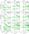 |
Fig. 2. Measured total XSB profiles from the deep XMM-Newton observation in the 0.7 − 1.2 keV band for each cluster and detector. Also shown are the independently measured background components, such as the astrophysical background (CXB, Eq. (3)), the instrumental background (IBKG, Eq. (1)), and for EPN also the expected out-of-time events (OOT). For visualization purposes, the thickness of the green crosses is reduced for > 2′. A logarithmic scale for the x-axis was used to highlight the cluster emission at small radii. The dashed vertical line shows the upper limit of the core region (< 100 kpc, Sect. 3.3.3). The scales between the dashed and dotted vertical lines are used for spectroscopy (Sect. 3.2). |
3.1.1. Instrumental background
For each detector, the XSB of the IBKG for the profile bin b is computed as follows:
where Ωb and ⟨tb⟩ are the surface area and average exposure time of the profile bin b. Here, we make use of the master-background-count map CMB, which was constructed out of the Filter-Wheel-Closed observations of XMM-Newton5 following the description of KOL21 (appendix C).
The scaling factor αClu in Eq. (1) is computed as:
where αoutFOV scales CMB to the total-count map CT using the counts within the outFOV area for the same energy band as the profile and  scales CMB to CT using the counts within the particle band6 of the same detector area as the entire profile of the corresponding cluster. Both methods are described in more detail in KOL21 (appendix B).
3.1.2. Astrophysical background
The CXB contribution is estimated from the CXB region (defined in Sect. 2.3) of the total-count map CT as follows:
![$$ \begin{aligned} S^\mathrm{CXB}&= \dfrac{1}{\Omega ^\mathrm{CXB} } \sum _p^N \dfrac{ M^\mathrm{CXB} }{ E } \left( C^\mathrm{T} - \alpha ^\mathrm{CXB} \, C^\mathrm{MB} \right) \text{,} \\ \sigma \left(S^\mathrm{CXB} \right)&= \dfrac{1}{\Omega ^\mathrm{CXB} } \left[ \sum _p^N \dfrac{ M^\mathrm{CXB} }{ E^2 } \left( C^\mathrm{T} + \left( \alpha ^\mathrm{CXB} \right)^2 \, C^\mathrm{MB} \right) \right]^{\frac{1}{2}} \nonumber \text{,} \end{aligned} $$](/articles/aa/full_html/2021/09/aa40657-21/aa40657-21-eq4.gif)
where MCXB, ΩCXB, and αCXB are the mask, the surface area, and the CMB-scaling factor of the CXB region. Given this definition, it follows that SCXB has the same value for all clusters for a given detector. In Fig. 2, we can see that the CXB (dashed lines) is the dominant background component and for very large radii it dominates the entire emission.
3.2. Spectroscopy
The spectrum extracted from a cluster is described with a one-temperature APEC7 model (Smith et al. 2001), where its free parameters are the temperature, redshift, metallicity, and normalization. Galactic absorption is taken into account via the photoelectric absorption model phabs, for which we use a hydrogen column density of NH = 4.59 × 1020 cm−2 as determined by Kalberla et al. (2005)8 for our XMM-Newton observations and the solar metallicity of Anders & Grevesse (1989).
For the spectral fitting we use the package XSPEC9 (v12.10.1f, Arnaud et al. 1996) in conjunction with the bayesian parameter estimation package BXA10 (v3.3, Buchner et al. 2014), which requires the use of cstat for the fit statistic of XSPEC and makes use of the nested sampling algorithm MULTINEST11 (v3.10, Feroz & Hobson 2008; Feroz et al. 2009, 2019) via the library PYMULTINEST12 (v2.9).
The CXB component of the energy spectrum is described with an APEC + phabs(APEC + powerlaw) model, which captures the emission of the local hot bubble, the Galactic halo, and extragalactic sources. For the APEC models, the metallicity and redshift are set to unity and zero, respectively (e.g., Snowden et al. 2000; Henley & Shelton 2013), and the photon index of the power law is fixed to 1.46 (e.g., Lumb et al. 2002; Moretti et al. 2003; De Luca & Molendi 2004). The galactic absorption is the same as for the cluster model. The best-fit values of the remaining five free model parameters are determined from a spectral analysis of the CXB region of the observation and are used as fixed parameters, when fitting the energy spectrum of a cluster. They are listed in Table A.1 and their posterior distributions are shown in Fig. A.3. The energy spectrum of the CXB region is shown in Fig. A.1 and the derived XSB of the three CXB model components are shown in Fig. A.4, which appear consistent with expectations.
Emission lines of the IBKG were identified and modeled following the XMM-ESAS documentation3 but also considering the studies of Leccardi & Molendi (2008), Kuntz & Snowden (2008), Mernier et al. (2015), and Gewering-Peine et al. (2017). The continuum of the HEB is modeled with a broken power law. Best-fit values are obtained by fitting the HEB continuum to the energy spectrum of the master-background-count map (defined in Sect. 3.1.1) for the same detector area as the source region; for example, a cluster profile bin or the CXB region. Thereby, energy ranges that contain known IBKG emission lines were ignored. The model parameters are fixed to these best-fit values, except for the normalization. For EPN, the HEB continuum model is used to describe the entire IBKG continuum, that is, including the SPB. For EMOS, the SPB continuum is described separately with a broken power law. We adopt the values of Leccardi & Molendi (2008) for the lower-energy slope and energy break parameter. The values of the high-energy slope and normalization are obtained from fitting the 5.0 − 11.2 keV band of the energy spectrum of the CXB region (Fig. A.1), because this energy band has a negligible contribution from the CXB for our data. During this fit, the normalization of the HEB continuum is fixed via the XSB in the 10.0 − 11.2 keV band measured from the outFOV area. When fitting the energy spectrum of a cluster profile bin or the CXB region, the normalization of the [HEB,IBKG] model for the [EMOS,EPN] detector remains the only free parameter of the IBKG continuum model.
3.2.1. Global values
To estimate the average spectroscopic temperature, redshift, and metallicity for each cluster, we model the energy spectrum over a broad profile region with respect to angular scale. To maximize the precision of those spectroscopic estimates, we set the maximum radius of this region to the largest possible angular scale, where the cluster XSB is still not significantly lower than the XSB of the CXB (estimated via Eq. (3)). This leads to radii of [2.0′,1.5′,1.0′] for clusters [A, B, C], respectively, which was revealed later in our analysis to correspond to ∼[0.7, 0.9, 0.7]×R500 (Table 3). For cluster A, the spectrum is shown in Fig. A.2. The limits are shown as dotted vertical lines in Fig. 2. The cluster core (< 100 kpc) was excluded from this analysis to avoid including the emission of potential cool cores.
We show our estimates for the redshift and metallicity parameters together with the temperature estimates in Table 1 and Fig. 3. For the temperature and redshift, we show different cases, where either all parameters are free (all free) or at least one other parameter is fixed to its default value (black dashed line), which we define in the following sections.
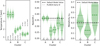 |
Fig. 3. Posterior distribution of temperature T, redshift z, and metallicity mZ after modeling the X-ray energy spectrum for a broad profile region of each cluster (Sect. 3.2.1). Thick and thin dashed green lines show median and 1σ levels. For the temperature and redshift, we show different cases, where either all parameters are free (all free) or at least one other parameter is fixed to the default value of our model, which is shown as a black dashed line in the middle and right panels. The gray dotted line in the middle panel shows the redshift estimate by PLIX2011 for cluster A based on the shallow XMM-Newton observation. |
Best-fit values and their 1σ levels of temperature T, redshift z, and metallicity mZ.
3.2.2. Redshift
We estimate the redshift of each cluster by modeling the X-ray energy spectrum of the broad profile region defined in Sect. 3.2.1, where the metallicity was fixed to our default value (mZ = 0.3, see Sect. 3.2.3). The results of the modeling are shown as mZ fixed case in Fig. 3 and Table 1. For clusters A and C, we obtain redshift estimates of z = 0.37 ± 0.01 and  , respectively. Both values are consistent with each other and also consistent with the value of z = 0.35 estimated by PLIX2011 (gray dotted line in the middle panel of Fig. 3). As cluster A is the brightest of the three clusters and its redshift estimate has the highest precision, we use its best-fit value (z = 0.365) in the following as the default value for our cluster emission models.
For cluster B, we estimate a redshift of z = 0.27 ± 0.02, which stands in strong tension with the redshifts of the other clusters, especially cluster A (∼5σ tension). This value would suggest that cluster B is actually not a member of the triple-cluster system, as it would be ∼350 Mpc closer to the observer in the line-of-sight (LoS) direction than the other two members. However, our redshift estimate of cluster B is based on modeling the cluster energy spectrum, which does not have any significant line emission from iron, with a one-temperature APEC model. This makes the redshift estimate unreliable.
3.2.3. Metallicity
To estimate the metallicity, we fixed the redshift to our default value (z = 0.365, see Sect. 3.2.2). This revealed that with the given data, it is not possible to properly constrain the metallicity for clusters B and C.
For cluster A, we obtain  . It is worth noting that this estimate does not show a significant degeneracy with the temperature and normalization parameters. This estimate is consistent with the common assumption of mZ = 0.3 for solar metallicity, which is based on previous cluster metallicity studies (e.g., Mernier et al. 201813). Hence, in the following, the metallicity of our cluster emission models is fixed to mZ = 0.3.
3.2.4. Measuring the cluster temperature profile
In Fig. 4, we show our spectroscopic temperature profiles, where redshift and metallicity were fixed to their default values (z = 0.365 and mZ = 0.3, see Sects. 3.2.2 and 3.2.3). The profiles are used for the joint fit in Sect. 3.3.5, where they are simultaneously fitted with the total XSB profiles. We limit the profile bins to angular scales of [95″,90″,65″] for clusters [A,B,C], respectively, which was revealed later in our analysis to correspond to ∼[0.5, 0.9, 0.8]×R500 (Table 3) since beyond this scale the amplitude of the cluster emission is at the same level as, or below, the amplitude of the CXB emission and our model of the CXB emission is not accurate enough to provide reliable measurements in this regime for a single profile bin.
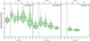 |
Fig. 4. Cluster temperature profiles: Posterior distribution of the temperature after modeling the X-ray energy spectrum of consecutive profile bins of each cluster. Thick and thin dash lines are median and 1σ levels. The dashed vertical line shows the upper limit of the core region (< 100 kpc, Sect. 3.3.3). |
3.3. Modeling
To model the X-ray emission of the gas in and around clusters, we used two different parametric models directly projected onto the sky. An important feature of this forward-fitting approach is that a model can be applied directly to the data. Both models provide a 3D radial profile for the electron number density ne and temperature T of a cluster assuming spherical symmetry and a hydrostatic equilibrium with only three free parameters, which will increase to five when including our model for the core region. As both models use different underlying physical assumptions, they can be considered as independent.
3.3.1. Isothermal beta-profile model
Our first model assumes that the gas temperature is constant (T(r3D) = Tiso) and the density profile can be described with a beta-profile (Cavaliere & Fusco-Femiano 1976):
![$$ \begin{aligned} n_{\rm e}(r_\mathrm{3D} ) = n_{\mathrm{e},0} \left[1+ \left( \frac{r_\mathrm{3D} }{r_{\rm c}} \right)^2\right]^{- \frac{3}{2}\beta } \text{,} \end{aligned} $$](/articles/aa/full_html/2021/09/aa40657-21/aa40657-21-eq12.gif)
where r3D is the profile radius from the cluster center. Hence, the free model parameters are: the temperature Tiso, the core radius rc, and the density profile normalization ne, 0. The slope β is kept fixed to a value of two-thirds in our study.
This model neglects that the radial temperature of clusters declines beyond their central parts towards the outskirts (e.g., Markevitch et al. 1998; Ghirardini et al. 2019). The statistical quality of our data (see the uncertainties on our temperature measurements in Fig. 4) prevents us from a complex modeling of the temperature shape14 (i.e., using an analytic function such as the one provided by Vikhlinin et al. 2006). We therefore restrict the complexity of this model via the assumption of an isothermal sphere, while for our second model, introduced in the following section, we use a different approach. Here, we purposefully exclude the cluster core, and we address it separately in Sect. 3.3.3.
3.3.2. Polytropic NFW-profile model
Our second model assumes that the dark matter density profile can be described with a NFW profile (Navarro et al. 1997). Its free parameters are the characteristic radius rs, where the profile slope changes, and the (dimensionless) concentration parameter cΔ. These define the reference radius RΔ = cΔ rs, where the mean matter density of the cluster halo is Δ times the critical density of the Universe ρc, resulting in an enclosed mass of  .
.
The model also assumes that the gas profile can be described with a polytropic gas model. Using the convention of Komatsu & Seljak (2001, hereafter KoSe01), the electron number density profile is defined as:
and the gas temperature profile as:
assuming the polytropic parameterization  with the polytropic index γ. The dimensionless gas profile yg is determined by solving the hydrostatic equilibrium equation (see Eq. (19) of KoSe01) and T0 is computed via Eq. (20) of KoSe01.
The parameterization of ne(r3D) and T(r3D) adds two more model parameters: ne, 0 and γ. The polytropic index is kept correlated to cΔ via the linear-fit formula of KoSe01 (Eq. (25)). Hence, the three free model parameters are: cΔ, rs, and ne, 0. Following the convention of KoSe01, we use Δ = 200.
3.3.3. Core region
Each cluster may contain a cool core, which cannot be adequately described by either of our two simple models (e.g., Hudson et al. 2010; Komatsu & Seljak 2001). To take such a contribution into account, we split each radial profile model into a “core” region and a “without-core” profile (Out):
where the core-region upper limit is defined as RCore = 100 kpc (which turns out to be ∼[0.1, 0.2, 0.2]×R500 for cluster [A,B,C], respectively) and ne, Core and TCore are two additional free parameters, giving five free parameters in total for each cluster model. Our model design can lead to a nonphysical discontinuity for the temperature and density between the core region and the without-core profile, especially for cool-core clusters. This is taken into account when we interpret the results. We do not expect that this profile separation creates a strong bias in our understanding of the without-core profile, because the core properties are typically not strongly correlated with it (e.g., Lau et al. 2015; McDonald et al. 2017).
3.3.4. Radial profile models
Based on the density and temperature profile of each model, we compute its corresponding volume emissivity profile as follows:
which follows the convention of the APEC plasma code, that is, using the hydrogen number density (nH) instead of ion number density (ni). We then compute the projected temperature profile in [keV] and the cluster XSB profile for each detector in instrumental units [cts s−1 deg−2] with the help of XMM-Newton response files extracted from the on-axis point of the observation. The projected temperature profile TEW is computed with the emission-weighted, projected 3D temperature profile T(Full)(r3D), and a cluster XSB profile SClu is computed with the projected volume emissivity profile ϵV(r3D), using the Abel transform for the projection, as explained in Appendix B, in both cases.
In order to compare the temperature profile model to the measurement, we have to fit it to the corresponding spectroscopic temperature profile (shown in Fig. 4). We note that a comparison between emission-weighted and spectroscopic temperatures can be biased but only if the gradient of the underlying 3D temperature is strong (e.g., Vikhlinin 2006). Based on results from Mazzotta et al. (2004), we expect that such a bias is much smaller than our measurement uncertainties, because our analysis reveals that each 3D temperature profile covers only a small temperature range within R500 (Sect. 3.4.2).
Additional operations are necessary in order to compare the cluster XSB profile models with their corresponding measured XSB profiles (shown in Fig. 2). First, the profile model is convolved with the XMM-Newton PSF  estimated for the detector position of the cluster center with the SAS task psfgen. Second, a CXB and a IBKG component are added, resulting in the following total XSB profile model of the profile bin b for a given detector:

where r⊥ is the profile radius from the cluster center within the projected plan, i.e., perpendicular to the LoS.
In Eq. (10), the IBKG component is defined with Eq. (1). The CXB component is modeled with a constant parameter SCXB for the entire profile, which is a reasonable assumption. We note that SCXB can include emission from other cluster members and the ISCM. To constrain it sufficiently well, it is important that XSB profiles extend to radii where the CXB emission dominates over other emissions. As for our analysis this happens beyond ∼4′≈1.3 Mpc (see Fig. 2), our profile region was defined to have a 6′ radius (≈1.9 Mpc) from the cluster center. The CXB component adds three more parameters to the XSB profile model (one per detector), resulting in eight free parameters for the entire model.
In order to use a Poisson likelihood during the fitting process, the XSB profile model is converted from count rate [cts s−1 deg−2] to the sum of total counts [cts] per profile bin as follows:
where Ωb is the surface area, ⟨tb⟩ the average exposure time, and  is the sum of counts expected from out-of-time events of EPN (and zero for the other detectors) for the profile bin b. We note that
  is a negligible component for our analysis (see bottom panels of Fig. 2).
3.3.5. Fitting
For each cluster of the triple system, we fit one model simultaneously to the radial XSB profiles of all detectors (Fig. 2) and the radial temperature profile (Fig. 4) via a maximum-likelihood estimation. The corresponding joint likelihood is computed as follows:
which sums up the logarithmic likelihoods of the XSB profiles and the temperature profile. NXXM = 3 is the number of XMM-Newton detectors. The logarithmic likelihood of the XSB profile of detector d is computed as follows:
Here, we compute the logarithmic probability of measuring the sum of total counts  for the XSB profile bin b of detector d given our model
  (Eq. (11)). The probability is computed with the Poisson distribution in natural logarithmic form, where all nonmodel-dependent terms are ignored because they are not relevant for the maximum-likelihood estimation. The logarithmic likelihood of the temperature profile is computed as follows:
Here, we compute the probability  of measuring the emission-weighted temperature for the profile bin b given our model
  .
.  is estimated with the normalized posterior distribution of the temperature obtained from the spectral fit shown in Fig. 4.
For our maximum-likelihood estimation, we derive the posterior distributions of our model parameters and the Bayesian evidence with the nested sampling Monte Carlo algorithm MLFRIENDS (Buchner 2014, 2019) using the Python package ULTRANEST15 (v2.2.0).
3.4. Results
3.4.1. Best-fit models and derived quantities
In Fig. 5, we compare our best-fit profile models with our data. This illustrates that both best-fit models, that is, the isothermal beta-profile and the polytropic NFW-profile model, can describe the measured profiles of all clusters rather well. In Table 2, we list the best-fit values of the cluster parameters of each model and in Fig. C.1 we show their corresponding posterior distributions. We should note that the free cluster parameters do not show any strong degeneracy with the free background-model parameters described in Sect. 3.3.4.
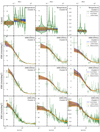 |
Fig. 5. Comparison of our measurement (green) of the XSB profiles (Fig. 2) and temperature profiles (Fig. 4) and their corresponding best-fit models (incl. 1σ level) for the isothermal beta-profile model (Sect. 3.3.1) in blue and for the polytropic NFW-profile model (Sect. 3.3.2) in orange. For visualization purposes, the thickness of the green crosses is reduced for > 2′. The posterior distributions of the best-fit model parameters are shown in Fig. C.1. The dashed vertical line shows the separation of the core region (< 100 kpc) and the without-core profile (Sect. 3.3.3). |
Best-fit values and 1σ levels of the free cluster parameters of both models.
For cluster C, the core-model parameters were not properly determined because of a lack of sufficient observational constraints, making the results dependent on their fit boundaries: [0.4, 10.0]×10−3 cm−3 for ne, Core and [0.5, 6.0] keV for TCore. However, those boundaries were chosen to be wide enough to encompass the expected range for clusters.
We use both best-fit models, that is, the isothermal beta-profile and the polytropic NFW-profile model, to derive important physical quantities, such as size, mass, luminosity, and average temperature for different apertures. Unsurprisingly, both models give consistent estimates. In Table 3, we list R500 and its associated angular scale (θ), total hydrostatic mass (Mt), and gas mass (Mgas). The same quantities for R200 are shown in Table C.1. This shows that cluster A is more than twice as massive as both other clusters combined based on their R500 values. The combined R200 mass of all three cluster remains below ∼1015 M⊙ (Table C.1). The R500 regions are not overlapping with each other (see Fig. 1) but the R200 region of cluster A has a small overlap with the R200 regions of the other clusters in the projected plan.
Median and 1σ levels of R500-related quantities.
In Table 4, we list the derived luminosities (L) for different apertures, which show that including or excluding the cluster core makes a significant difference, especially for cluster A. In Table 5, we list the derived temperature for different apertures. The estimates for the < 0.3 Mpc region are used for the comparison with a temperature–luminosity scaling relation (Sect. 4.1). The RCore − RSpec. aperture uses the same radial limit as the broad profile range, which was used to estimate average cluster properties (Sect. 3.2.1). The values from this direct measurement (Table 1) and the best-fit models are consistent with each other.
Median and 1σ levels of the luminosity in the 0.5 − 2.0 keV band for different apertures.
Median and 1σ levels of the temperature [keV] for different aperture.
3.4.2. Entropy and the cluster core
With the best-fit model of the 3D gas density and temperature profiles, we can derive the X-ray entropy profile as follows:
All three profiles are shown for each cluster in Fig. 6. The core region (< 100 kpc) is only shown in a plot insert to visually separate it from the without-core profile (≥100 kpc) because our model can induce nonphysical discontinuities between both regions, especially for cool-core clusters (Sect. 3.3.3). For cluster C, the core region is not shown because its parameters were not properly determined (Table 2).
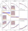 |
Fig. 6. Electron number density, temperature, and entropy profiles of the best-fit model up to R200. Blue areas and dash curves show the isothermal beta-profile model (Sect. 3.3.1). Orange areas and dotted curves show the polytropic NFW-profile model (Sect. 3.3.2). Curves show the median and areas show the 1σ level of the models. The main plots show the without-core profiles (≥100 kpc) and the plot inserts show the core region (< 100 kpc). This visual separation is necessary because our model can create nonphysical discontinuities between both regions, especially for cool-core clusters (Sect. 3.3.3). For each cluster, all inserts have the same x-axis range but for clarity the tick labels are only shown in the top row. The core region of cluster C is not shown because its core-region parameters were not properly determined (Table 2). For the entropy profiles, the black lines show the self-similar prediction by Voit et al. (2005), K(r3D) = 1.32 K200 (r3D/R200)1.1. |
For the entropy profiles in Fig. 6, we also show a self-similar model by Voit et al. (2005) using black lines, namely K(r3D) = 1.32 K200 (r3D/R200)1.1, which does not take stellar or active galactic nucleus (AGN) feedback into account. For cluster A, the entropy profile follows this model on most scales rather well (apart from the offset in the normalisation). Moreover, its core appears to be denser and cooler than the without-core profile, which can be deduced from the best-fit values of its isothermal beta-profile model (Table 2). These observations suggest that cluster A most likely falls into the class of relaxed cool-core clusters. For cluster B, the entropy profile flattens around ∼0.5 R500 suggesting an entropy excess towards the cluster center with respect to the self-similar model. Moreover, there is no significant discontinuity between core region and the without-core profile, suggesting that the core is neither denser nor cooler than the without-core profile. These observations indicate that cluster B falls rather into the class of disturbed noncool-core clusters. Our tentative classification for clusters A and B is also supported by a comparison with previous entropy measurements with large cluster samples (Cavagnolo et al. 2009; Ghirardini et al. 2017). For cluster C, it appears that the entropy profile flattens around ∼0.5 R500 but due to the unconstrained core region, we cannot assess how density and temperature change towards the cluster center and therefore we refrain from making any classification.
4. Discussion
4.1. Cluster properties in respect to scaling relations
In Fig. 7, we compare the temperature T, luminosity L (0.5 − 2.0 keV), and gas mass Mgas derived from our best-fit models with three scaling relations derived from the 100 brightest clusters of the XXL sample (Sereno et al. 2019). The redshift and mass of our clusters fall well within the covered range of this sample. All clusters follow the Mgas − L relation relatively well. For the T − L and T − Mgas relations, cluster C shows the strongest disagreement. However, when compared with the actual measurements for the XXL sample (Fig. 2 of Sereno et al. 2019), cluster C does not appear as an outlier in this sample. This indicates that all clusters of our system have consistent properties with respect to the XXL 100 brightest clusters. As about 80% of the clusters in the sample are identified as single clusters, the consistency with them may indicate that our clusters have similar properties to typical single clusters.
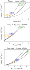 |
Fig. 7. Comparison of derived cluster parameters with scaling relations derived from the 100 brightest clusters of the XXL sample (Sereno et al. 2019). The luminosity is given for the 0.5 − 2.0 keV band and the aperture for all quantities is R < 0.3 Mpc. The black solid and dashed curves show the median and intrinsic scatter of the scaling relations, respectively. Green, blue, and orange contours correspond to clusters A, B, and C, respectively. The contours show the 1σ and 2σ levels of the isothermal beta-profile model. As the polytropic NFW-profile model has almost the same contours, they are omitted for clarity. |
4.2. Measurement comparison
In Fig. 8, we compare our estimates for R500, Mt, 500, Mgas, 500, TX, and L500 with those from PLIX2011, which only used the shallow observation for their analysis. There, we can see that their R500 estimate is significantly different from ours, which reflects the different approaches in estimating R500. To have a fair comparison of R500-dependent quantities, we use their measurement of R500, symbolized as  . Moreover, for increased consistency with the measurements of PLIX2011, TX was estimated for
  and the luminosity
  was estimated for the 0.1 − 2.4 keV band from our best-fit models.
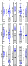 |
Fig. 8. Comparison of cluster parameters derived from our best fit of the isothermal beta-profile model in blue and estimated by PLIX2011 (Table 2) in gray. As the results for the polytropic NFW-profile model are almost the same, they are omitted for clarity. The blue thick and thin dash lines are the median and 1σ levels of our model. The gray areas show the 1σ levels of PLIX2011, except for R500, which was not provided. Top, middle, and bottom rows: clusters A, B, and C, respectively. See Sect. 3.4.1 for more details. |
In respect to the R500-dependent quantities, we can see in Fig. 8 that for clusters B and C the measurements of PLIX2011 are consistent with ours, except for Mgas of cluster B. We note that PLIX2011 state that they did not account for systematic uncertainties related to redshift uncertainties or high background levels, which likely means their errors are underestimated. For instance, their uncertainties for cluster A appear to be of similar size to ours, while they only used the shallow observation, which has an approximately four times lower exposure time than the deep observation. Even taking this into account cannot explain the discrepancy for the estimates of Mt, 500, Mgas, 500, and TX for cluster A. The difference might be due to the choice of approach in the spatial and spectral modeling of the cluster emission. Most notably, PLIX2011 subtracted the IBKG beforehand and left the power-law index of the extragalactic CXB model free and used the MEKAL model for the cluster emission.
4.3. Interactions between clusters
One way to search for signs of interaction between clusters is to detect enhanced (or irregular) X-ray emission between clusters (e.g., Planck Collaboration Int. VI 2013). For the present triple system, this requires modeling the emission of all clusters simultaneously, because they all have similar angular distances and are distributed in the projected plane almost like an equilateral triangle with an edge length of ∼2.0 Mpc (∼6′), which does not rule out the scenario that all three clusters have a significant interaction with each other at the same time. However, when comparing our best-fit model to a smoothed count-rate image for each detector, no significant deviation from the total signal of all clusters, the CXB, and the IBKG was detected. This could mean that there has not been any direct cluster interaction so far, which would not be unexpected because none of the clusters have overlapping R500 regions. This would also be in line with the finding that all clusters are consistent with the scaling relation of the XXL 100 brightest clusters, where 80% of them are not associated with a multi-cluster system (Sect. 4.1). However, our X-ray data alone are not sensitive enough to be used to measure such an excess signal, because the XSB of each cluster drops below the CXB already within its R500 region. Hence, a joint analysis of X-ray and tSZ data would be required to increase the sensitivity and potentially detect signs of interactions between clusters, because the tSZ effect is more sensitive to the emission in the cluster outskirts (e.g., Eckert et al. 2017). The latter makes such a joint analysis particularly suitable for revealing the presence and the properties of WHIM within the system.
4.4. Comparison of Planck-detected triplet systems
The triple system (hereafter TS1) analyzed by Planck Collaboration Int. VI (2013) (PLCK G214.6+36.9) and that analyzed in this work (hereafter TS2) are the only two known Planck-detected triplet-cluster systems to date. Nevertheless, both cases might only be apparent triplet systems, because it remains unclear as to whether or not all members are at the same redshift. TS1 is more distant than TS2 to the observer, with redshifts of z ≈ 0.45 and z ≈ 0.37, respectively. TS1 is also more massive with about twice as much accumulative R500 mass, which is almost evenly distributed among the SC members with a proportion of ∼1 : 1.1 : 1.4 for clusters A, B, and C, respectively, while for TS2 the proportion is ∼7 : 2 : 1. For TS2, one cluster is more than twice as massive as both other clusters combined. Both systems contain one relaxed cluster with a cool core (cluster A in both cases) while the other clusters appear to be more disturbed and without a cool core (or remain without classification), based on the derived gas density, temperature, and entropy profiles from X-ray data. It is interesting to note that for TS1 the relaxed cool-core cluster is the least massive, while for TS2 it is the most massive.
The clusters of TS1 are distributed in the projected plane almost like an isosceles triangle with cluster C at the top and at a distance of ∼2.5 Mpc from the other clusters, which are both separated by only ∼1.1 Mpc. The clusters of TS2 have more similar angular distances between each other and are distributed in the projected plane almost like an equilateral triangle with an edge length of ∼2.0 Mpc. For TS1, the two clusters closest to each other have overlapping R500 regions in the projected plane but no enhanced X-ray emission – an indication of interaction – was detected between them. For TS2, none of the clusters have overlapping R500 regions and no enhanced X-ray emission was detected between them.
This comparison shows that none of the systems show signs of cluster interactions and that they have quite different configurations based on their X-ray data. This suggests rather different cluster merger scenarios for both SCs, under the assumption that all clusters of each SC are at about the same redshift, and are indeed merging systems.
5. Summary
Multi-cluster systems are an important structure formation probe in the Universe. Two triplet-cluster systems have been discovered from the follow-up campaign of Planck-detected clusters (Planck Collaboration VIII 2011; Planck Collaboration IX 2011) with XMM-Newton. For one system, PLCK G214.6+36.9, a multi-wavelength analysis has already been conducted (Planck Collaboration Int. VI 2013). In the present work, we study the X-ray emission observed by XMM-Newton of the other system, PLCK G334.8-38.0, which represents the first step in a multi-wavelength study.
Our X-ray analysis reveals that the system is located at z = 0.37 ± 0.01 (Sect. 3.2.2). Although, our measurement is not precise enough to confirm that all three clusters are part of the same system, meaning that a subsequent study with optical spectroscopy is required for verification. The X-ray analysis also provides a temperature profile for each cluster (Sect. 3.2.4) and supports the assumption of 0.3 times solar metallicity for their ICM (Sect. 3.2.3).
We simultaneously fitted the spectroscopic temperature profile (Fig. 4) with the XSB profiles of all three XMM-Newton detectors (Fig. 2) in order to constrain the physical properties of each cluster (Sect. 3.3). This revealed a hydrostatic mass of ∼[2.5, 0.7, 0.3]×1014 M⊙ and an average temperature of ∼[3.9, 2.3, 1.6] keV) within R500 for clusters A, B, and C, respectively (Sect. 3.4.1). Hence, cluster A is more than twice as massive as both other clusters combined, showing an uneven distribution of mass within the system, whose total mass is below ∼1015 M⊙ based on the M200 mass of all clusters.
With our best-fit model, we derive the X-ray entropy profile for each cluster (Sect. 3.4.2). This suggests that the brightest/most massive cluster A appears to be a relaxed cool-core cluster, which is also supported by the temperature decrease and gas density increase towards its center (Fig. 6). The second brightest and second-most massive cluster (B) appears to be a disturbed noncool-core cluster and the X-ray signal of the third cluster (C) was too weak to make such a classification.
No sign of cluster interaction was found when searching for enhanced X-ray emission between the clusters, which is not unexpected, because none of the clusters have overlapping R500 regions (Sect. 4.3). This is also in line with the consistency of cluster properties with scaling relations based on single clusters (Sect. 4.1). However, our X-ray data alone do not permit us to detect significant cluster emission beyond R500. Hence, a joint analysis of X-ray and tSZ is required, which may also reveal the presence of WHIM within the system.
Comparison of the two Planck-detected triplet-cluster systems reveals that neither shows signs of cluster interactions and that the two have quite different configurations based on their X-ray data alone (Sect. 4.4). This suggests rather different cluster merger scenarios, under the assumption that all clusters of each system are at about the same redshift.
XMM-Newton Extended Source Analysis Software, https://www.cosmos.esa.int/web/xmm-newton/xmm-esas
Using atomic database ATOMDB v3.0.9, http://www.atomdb.org
We note that Mernier et al. (2018) used a different solar abundance (Lodders et al. 2009), which may introduce some bias. Fortunately, the best-fit values of temperature and redshift do not change significantly when using their solar abundance instead, i.e., such a potential bias is much smaller than our measurement uncertainties. Moreover, those best-fit values also do not change significantly when the metallicity becomes a free parameter, as shown in Fig. 3.
Acknowledgments
The authors acknowledge helpful discussion with F. Gastaldello, S. Molendi, and the members of the ByoPiC project (https://byopic.eu/team). We thank the referee for the useful comments. This research has been supported by the funding for the ByoPiC project from the European Research Council (ERC) under the European Union’s Horizon 2020 research and innovation program grant agreement ERC-2015-AdG 695561 and CNES. This publication used observations obtained with XMM-Newton (https://www.cosmos.esa.int/web/xmm-newton), an ESA science mission with instruments and contributions directly funded by ESA Member States and NASA. This research has made use of data obtained from the 3XMM XMM-Newton serendipitous source catalog compiled by the 10 institutes of the XMM-Newton Survey Science Centre selected by ESA. This research has made also use of the application package CIAO (v4.11), provided by the Chandra X-ray Center (CXC), and the software packages FTOOLS (https://heasarc.gsfc.nasa.gov/docs/software/ftools) (v6.26, Blackburn 1995) the Python environment IPYTHON (https://ipython.org) (Pérez & Granger 2007) and JUPYTER NOTEBOOK (https://jupyter.org), the community-developed Python packages of ASTROPY (https://www.astropy.org) (Astropy Collaboration 2013, 2018), core packages of SCIPY (https://www.scipy.org/) (a Python-based ecosystem of open-source software, Jones et al. 2001), such as NUMPY (https://www.numpy.org) (Oliphant 2006; van der Walt et al. 2011), and MATPLOTLIB (https://matplotlib.org) (Hunter 2007), and the Python package CORNER (https://github.com/dfm/corner.py) (Foreman-Mackey 2016).
References
- Akamatsu, H., Fujita, Y., Akahori, T., et al. 2017, A&A, 606, A1 [NASA ADS] [CrossRef] [EDP Sciences] [Google Scholar]
- Anders, E., & Grevesse, N. 1989, Geochim. Cosmochim. Acta, 53, 197 [Google Scholar]
- Araya-Melo, P. A., Reisenegger, A., Meza, A., et al. 2009, MNRAS, 399, 97 [Google Scholar]
- Arnaud, K. A. 1996, in Astronomical Data Analysis Software and Systems V, eds. G. H. Jacoby, & J. Barnes, ASP Conf. Ser., 101, 17 [Google Scholar]
- Astropy Collaboration (Robitaille, T. P., et al.) 2013, A&A, 558, A33 [NASA ADS] [CrossRef] [EDP Sciences] [Google Scholar]
- Astropy Collaboration (Price-Whelan, A. M., et al.) 2018, AJ, 156, 123 [Google Scholar]
- Blackburn, J. K. 1995, in Astronomical Data Analysis Software and Systems IV, eds. R. A. Shaw, H. E. Payne, & J. J. E. Hayes, ASP Conf. Ser., 77, 367 [Google Scholar]
- Bonjean, V., Aghanim, N., Salomé, P., Douspis, M., & Beelen, A. 2018, A&A, 609, A49 [NASA ADS] [CrossRef] [EDP Sciences] [Google Scholar]
- Buchner, J. 2014, Stat. Comput., 26, 383 [Google Scholar]
- Buchner, J. 2019, PASP, 131, 108005 [Google Scholar]
- Buchner, J., Georgakakis, A., Nandra, K., et al. 2014, A&A, 564, A125 [NASA ADS] [CrossRef] [EDP Sciences] [Google Scholar]
- Cautun, M., van de Weygaert, R., Jones, B. J. T., & Frenk, C. S. 2014, MNRAS, 441, 2923 [NASA ADS] [CrossRef] [Google Scholar]
- Cavagnolo, K. W., Donahue, M., Voit, G. M., & Sun, M. 2009, ApJS, 182, 12 [NASA ADS] [CrossRef] [Google Scholar]
- Cavaliere, A., & Fusco-Femiano, R. 1976, A&A, 500, 95 [NASA ADS] [Google Scholar]
- Cen, R., & Ostriker, J. P. 1999, ApJ, 514, 1 [NASA ADS] [CrossRef] [Google Scholar]
- Cen, R., & Ostriker, J. P. 2006, ApJ, 650, 560 [NASA ADS] [CrossRef] [Google Scholar]
- Chiappetti, L., Clerc, N., Pacaud, F., et al. 2013, MNRAS, 429, 1652 [NASA ADS] [CrossRef] [Google Scholar]
- de Filippis, E., Schindler, S., & Erben, T. 2005, A&A, 444, 387 [NASA ADS] [CrossRef] [EDP Sciences] [Google Scholar]
- De Luca, A., & Molendi, S. 2004, A&A, 419, 837 [NASA ADS] [CrossRef] [EDP Sciences] [Google Scholar]
- Dolag, K., Komatsu, E., & Sunyaev, R. 2016, MNRAS, 463, 1797 [Google Scholar]
- Eckert, D., Ettori, S., Pointecouteau, E., et al. 2017, Astron. Nachr., 338, 293 [NASA ADS] [CrossRef] [Google Scholar]
- Einasto, J., Joeveer, M., & Saar, E. 1980, MNRAS, 193, 353 [NASA ADS] [CrossRef] [Google Scholar]
- Feroz, F., & Hobson, M. P. 2008, MNRAS, 384, 449 [NASA ADS] [CrossRef] [Google Scholar]
- Feroz, F., Hobson, M. P., & Bridges, M. 2009, MNRAS, 398, 1601 [NASA ADS] [CrossRef] [Google Scholar]
- Feroz, F., Hobson, M. P., Cameron, E., & Pettitt, A. N. 2019, Open J. Astrophys., 2, 10 [Google Scholar]
- Foreman-Mackey, D. 2016, J. Open Source Softw., 1, 24 [Google Scholar]
- Gewering-Peine, A., Horns, D., & Schmitt, J. H. M. M. 2017, JCAP, 2017, 036 [CrossRef] [Google Scholar]
- Ghirardini, V., Ettori, S., Amodeo, S., Capasso, R., & Sereno, M. 2017, A&A, 604, A100 [NASA ADS] [CrossRef] [EDP Sciences] [Google Scholar]
- Ghirardini, V., Eckert, D., Ettori, S., et al. 2019, A&A, 621, A41 [NASA ADS] [CrossRef] [EDP Sciences] [Google Scholar]
- Giodini, S., Pierini, D., Finoguenov, A., et al. 2009, ApJ, 703, 982 [NASA ADS] [CrossRef] [Google Scholar]
- Govoni, F., Orrù, E., Bonafede, A., et al. 2019, Science, 364, 981 [NASA ADS] [CrossRef] [Google Scholar]
- Henley, D. B., & Shelton, R. L. 2013, ApJ, 773, 92 [NASA ADS] [CrossRef] [Google Scholar]
- Hickstein, D. D., Gibson, S. T., Yurchak, R., Das, D. D., & Ryazanov, M. 2019, Rev. Sci. Instrum., 90, 065115 [NASA ADS] [CrossRef] [Google Scholar]
- Hudson, D. S., Mittal, R., Reiprich, T. H., et al. 2010, A&A, 513, A37 [NASA ADS] [CrossRef] [EDP Sciences] [Google Scholar]
- Hunter, J. D. 2007, Comput. Sci. Eng., 9, 90 [NASA ADS] [CrossRef] [Google Scholar]
- Jones, E., Oliphant, T., Peterson, P., et al. 2001, SciPy: Open Source Scientific Tools for Python [Google Scholar]
- Kalberla, P. M. W., Burton, W. B., Hartmann, D., et al. 2005, A&A, 440, 775 [NASA ADS] [CrossRef] [EDP Sciences] [Google Scholar]
- Kéruzoré, F., Mayet, F., Pratt, G. W., et al. 2020, A&A, 644, A93 [CrossRef] [EDP Sciences] [Google Scholar]
- Kolodzig, A., Gilfanov, M., Hütsi, G., & Sunyaev, R. 2017, MNRAS, 466, 3035 [NASA ADS] [CrossRef] [Google Scholar]
- Komatsu, E., & Seljak, U. 2001, MNRAS, 327, 1353 [Google Scholar]
- Kravtsov, A. V., & Borgani, S. 2012, ARA&A, 50, 353 [NASA ADS] [CrossRef] [Google Scholar]
- Kuntz, K. D., & Snowden, S. L. 2008, A&A, 478, 575 [NASA ADS] [CrossRef] [EDP Sciences] [Google Scholar]
- Lau, E. T., Nagai, D., Avestruz, C., Nelson, K., & Vikhlinin, A. 2015, ApJ, 806, 68 [NASA ADS] [CrossRef] [Google Scholar]
- Leccardi, A., & Molendi, S. 2008, A&A, 486, 359 [NASA ADS] [CrossRef] [EDP Sciences] [Google Scholar]
- Lodders, K., Palme, H., & Gail, H. P. 2009, Landolt-Bornstein, 4B, 712 [Google Scholar]
- Lumb, D. H., Warwick, R. S., Page, M., & De Luca, A. 2002, A&A, 389, 93 [NASA ADS] [CrossRef] [EDP Sciences] [Google Scholar]
- Luo, B., Brandt, W. N., Xue, Y. Q., et al. 2017, ApJS, 228, 2 [Google Scholar]
- Markevitch, M., Forman, W. R., Sarazin, C. L., & Vikhlinin, A. 1998, ApJ, 503, 77 [NASA ADS] [CrossRef] [Google Scholar]
- Martizzi, D., Vogelsberger, M., Artale, M. C., et al. 2019, MNRAS, 486, 3766 [Google Scholar]
- Mazzotta, P., Rasia, E., Moscardini, L., & Tormen, G. 2004, MNRAS, 354, 10 [NASA ADS] [CrossRef] [Google Scholar]
- McDonald, M., Allen, S. W., Bayliss, M., et al. 2017, ApJ, 843, 28 [NASA ADS] [CrossRef] [Google Scholar]
- Mernier, F., de Plaa, J., Lovisari, L., et al. 2015, A&A, 575, A37 [NASA ADS] [CrossRef] [EDP Sciences] [Google Scholar]
- Mernier, F., Biffi, V., Yamaguchi, H., et al. 2018, Space Sci. Rev., 214, 129 [NASA ADS] [CrossRef] [Google Scholar]
- Molnar, S. M., Hearn, N., Haiman, Z., et al. 2009, ApJ, 696, 1640 [NASA ADS] [CrossRef] [Google Scholar]
- Moretti, A., Campana, S., Lazzati, D., & Tagliaferri, G. 2003, ApJ, 588, 696 [NASA ADS] [CrossRef] [Google Scholar]
- Navarro, J. F., Frenk, C. S., & White, S. D. M. 1997, ApJ, 490, 493 [NASA ADS] [CrossRef] [Google Scholar]
- Nelson, K., Lau, E. T., Nagai, D., Rudd, D. H., & Yu, L. 2014, ApJ, 782, 107 [NASA ADS] [CrossRef] [Google Scholar]
- Oliphant, T. E. 2006, A guide to NumPy, Vol. 1 (USA: Trelgol Publishing) [Google Scholar]
- Oort, J. H. 1983, ARA&A, 21, 373 [NASA ADS] [CrossRef] [Google Scholar]
- Pérez, F., & Granger, B. E. 2007, Comput. Sci. Eng., 9, 21 [Google Scholar]
- Planck Collaboration VIII. 2011, A&A, 536, A8 [NASA ADS] [CrossRef] [EDP Sciences] [Google Scholar]
- Planck Collaboration IX. 2011, A&A, 536, A9 [NASA ADS] [CrossRef] [EDP Sciences] [Google Scholar]
- Planck Collaboration XIII. 2016, A&A, 594, A13 [NASA ADS] [CrossRef] [EDP Sciences] [Google Scholar]
- Planck Collaboration XXII. 2016, A&A, 594, A22 [NASA ADS] [CrossRef] [EDP Sciences] [Google Scholar]
- Planck Collaboration Int. VI. 2013, A&A, 550, A132 [NASA ADS] [CrossRef] [EDP Sciences] [Google Scholar]
- Power, C., Elahi, P. J., Welker, C., et al. 2020, MNRAS, 491, 3923 [Google Scholar]
- Raychaudhury, S., Fabian, A. C., Edge, A. C., Jones, C., & Forman, W. 1991, MNRAS, 248, 101 [NASA ADS] [Google Scholar]
- Roncarelli, M., Cappelluti, N., Borgani, S., Branchini, E., & Moscardini, L. 2012, MNRAS, 424, 1012 [NASA ADS] [CrossRef] [Google Scholar]
- Rosen, S. R., Webb, N. A., Watson, M. G., et al. 2016, A&A, 590, A1 [NASA ADS] [CrossRef] [EDP Sciences] [Google Scholar]
- Ryu, D., Kang, H., Hallman, E., & Jones, T. W. 2003, ApJ, 593, 599 [NASA ADS] [CrossRef] [Google Scholar]
- Sarazin, C. L. 1988, X-ray Emission From Clusters of Galaxies [Google Scholar]
- Sarazin, C. L. 2002, in The Physics of Cluster Mergers, eds. L. Feretti, I. M. Gioia, & G. Giovannini, Astrophys. Space Sci. Libr., 272, 1 [Google Scholar]
- Sereno, M., Ettori, S., Eckert, D., et al. 2019, A&A, 632, A54 [NASA ADS] [CrossRef] [EDP Sciences] [Google Scholar]
- Shapley, H. 1930, Harvard College Obs. Bull., 874, 9 [NASA ADS] [Google Scholar]
- Shi, X., Nagai, D., Aung, H., & Wetzel, A. 2020, MNRAS, 495, 784 [NASA ADS] [CrossRef] [Google Scholar]
- Simionescu, A., Ettori, S., Werner, N., et al. 2021, Exp. Astron., in press [arXiv: 1908.01778] [Google Scholar]
- Smith, R. K., Brickhouse, N. S., Liedahl, D. A., & Raymond, J. C. 2001, ApJ, 556, L91 [NASA ADS] [CrossRef] [Google Scholar]
- Snowden, S. L., Freyberg, M. J., Kuntz, K. D., & Sanders, W. T. 2000, ApJS, 128, 171 [NASA ADS] [CrossRef] [Google Scholar]
- Snowden, S. L., Collier, M. R., & Kuntz, K. D. 2004, ApJ, 610, 1182 [Google Scholar]
- Tanimura, H., Aghanim, N., Douspis, M., Beelen, A., & Bonjean, V. 2019, A&A, 625, A67 [NASA ADS] [CrossRef] [EDP Sciences] [Google Scholar]
- Tozzi, P., Scharf, C., & Norman, C. 2000, ApJ, 542, 106 [NASA ADS] [CrossRef] [Google Scholar]
- Ulmer, M. P., Kinzer, R., Cruddace, R. G., et al. 1979, ApJ, 227, L73 [NASA ADS] [CrossRef] [Google Scholar]
- van der Walt, S., Colbert, S. C., & Varoquaux, G. 2011, Comput. Sci. Eng., 13, 22 [Google Scholar]
- Vikhlinin, A. 2006, ApJ, 640, 710 [NASA ADS] [CrossRef] [Google Scholar]
- Vikhlinin, A., Kravtsov, A., Forman, W., et al. 2006, ApJ, 640, 691 [NASA ADS] [CrossRef] [Google Scholar]
- Voit, G. M., Kay, S. T., & Bryan, G. L. 2005, MNRAS, 364, 909 [NASA ADS] [CrossRef] [Google Scholar]
- Werner, N., Finoguenov, A., Kaastra, J. S., et al. 2008, A&A, 482, L29 [NASA ADS] [CrossRef] [EDP Sciences] [Google Scholar]
- Zhang, C., Churazov, E., Dolag, K., Forman, W. R., & Zhuravleva, I. 2020, MNRAS, 494, 4539 [NASA ADS] [CrossRef] [Google Scholar]
Appendix A: Energy spectrum fit of the CXB
Figure A.1 shows the energy spectrum of the CXB region with our best-fit model, described in Sect. 3.2. The posterior distributions of its free parameters are shown in Figure A.3. The best-fit values of its CXB-component parameters are listed in Table A.1 and their derived XSB in the 0.5 − 2.0 keV band are shown in Figure A.4. Figure A.2 shows an energy spectrum of cluster A, where our best-fit CXB model was used as fixed model.
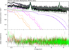 |
Fig. A.1. Energy spectrum of the CXB region with the best-fit model of all XMM-Newton detectors of the deep observation. The data points of EMOS1, EMOS2, and EPN are light gray, black, and dark gray in the upper panel, and black, red, and green in the lower panel, respectively. The model curves of EMOS1, EMOS2, and EPN are solid, dashed, and dot-dashed, respectively (mostly overlapping for the EMOS detectors). For each detector, the total model is shown as a blue curve, and the models of the CXB components, namely the local hot bubble, the Galactic halo, and the extragalactic emission are shown as orange, magenta, and violet curves, respectively. The [HEB,IBKG] and SPB models are shown as green and black curves, respectively (Sect. 3.2). |
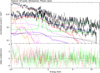 |
Fig. A.2. Energy spectrum of cluster A for its profile region 19″ − 2.0′≈(0.1 − 0.7)×R500 with the best-fit model of all XMM-Newton detectors of the deep observation. The same format is used here as for Figure A.1; additionally a cluster model is shown in red for each detector. Here, our best-fit CXB model (Table A.1) is used as a fixed model to determine the cluster model, as described in Sect. 3.2. |
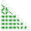 |
Fig. A.3. Posterior distribution of the free model parameters of each of the CXB components, namely the local hot bubble (LHB), the Galactic halo (GaH), and the extragalactic emission (ExG), and the [HEB,IBKG] normalization of each XMM-Newton detector after modeling the X-ray energy spectrum of the CXB region (see Figure A.1 and Sect. 3.2). For the 2D histograms, contours show the 1σ, 2σ, and 3σ levels. For the 1D histograms, dashed lines show the median and 1σ levels. Temperature parameters (T) are shown in units of keV and normalization parameters (e.g., K) are shown in decadic logarithm and units of log10(deg−2). The corresponding values of the XSB for the CXB components are shown in Figure A.4. |
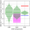 |
Fig. A.4. XSB of the CXB components, the local hot bubble (LHB), the Galactic halo (GaH), and the extragalactic emission (ExG), derived from the X-ray energy spectrum fit of the CXB region (Figure A.3). Thick and thin dashed lines are median and 1σ and 2σ levels. For GaH, the magenta bar shows the GaH measurement by Henley & Shelton (2013) for the southern galactic hemisphere. For ExG, the red bar shows the ExG measurement by Kolodzig et al. (2017) using the shallower survey XBOOTES, and the blue line shows the expected contribution of unresolved point sources in our observation using the log N − log S of Luo et al. (2017). These two reference values can be seen as upper and lower limits, respectively. |
Best-fit values and their 1σ uncertainties of the free CXB model parameters.
Appendix B: Profile projection onto the sky
We compute the projection along the LoS direction (r∥) of the profile Q(r3D) via the abel transform 𝒜:
with the coordinate convention:  is the radial coordinate in 3D space (r∥,rx,ry), r∥ is the coordinate in the LoS direction, and
  is the radial coordinate in the projected plane (rx,ry). The integration is done numerically via the Python package PYABEL16 (Hickstein et al. 2019), which also requires limiting the projection to a maximum radius (rmax); it is set to be three times the radius of the outermost profile bin (rmax = 3 rlast), because for this case, our numerical solution is consistent within ∼1.5 % with the analytical solution of the projection of ϵV(r3D) for the isothermal beta-profile model with β = 2/3. As revealed later in our analysis, this is significant lower than our statistical uncertainty of measuring the XSB profile (≈20 %) and the temperature profiles. We note that using much smaller values of rmax, such as rmax = rlast, is not recommended, because it makes the numerical solution highly inaccurate for the outer part (> rlast/3) of the profile.
Appendix C: Results of the radial profile fit
In Figure C.1 we show the posterior distribution of free cluster parameters of the best-fit models shown in Figure 5. We use those best-file models to derive R200 and its associated angular scale (θ), total hydrostatic mass (Mt), and gas mass (Mgas), which are shown in Table C.1. The same quantities for R500 are shown in Table 3.
Same as Table 3 for R200-related quantities.
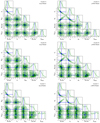 |
Fig. C.1. Posterior distribution of free cluster-model parameters from the joint fit of radial T and XSB profiles. Top, middle, and bottom rows correspond to clusters A, B, and C, respectively. Left column: Isothermal beta-profile model (Sect. 3.3.1). Right column: Polytropic NFW-profile model (Sect. 3.3.2). The blue solid lines show the median of each posterior distribution. For the 2D histograms, contours show the 1σ, 2σ, and 3σ levels. For the 1D histograms, dashed lines show 1σ levels. The free background-model parameters are omitted for clarity but they do not show any degeneracy with the cluster-model parameters. |
All Tables
Best-fit values and their 1σ levels of temperature T, redshift z, and metallicity mZ.
Median and 1σ levels of the luminosity in the 0.5 − 2.0 keV band for different apertures.
All Figures
|
Fig. 1. X-ray and tSZ emission of the triplet-cluster system PLCK G334.8-38.0. Left: XMM-Newton background-subtracted, detector-averaged count-rate map for 0.7 − 1.2 keV (masked and smoothed with a 15″ wide Gaussian kernel). Middle: Planck tSZ signal (Planck Collaboration XXII 2016). Right: X-ray source mask. Radial profiles are extracted from the cluster profile region and the supercluster zone was designed to enclose all three of those regions. The CXB region is used to study the astrophysical background. Further details of the different regions are given in Sect. 2.3. |
| In the text | |
|
Fig. 2. Measured total XSB profiles from the deep XMM-Newton observation in the 0.7 − 1.2 keV band for each cluster and detector. Also shown are the independently measured background components, such as the astrophysical background (CXB, Eq. (3)), the instrumental background (IBKG, Eq. (1)), and for EPN also the expected out-of-time events (OOT). For visualization purposes, the thickness of the green crosses is reduced for > 2′. A logarithmic scale for the x-axis was used to highlight the cluster emission at small radii. The dashed vertical line shows the upper limit of the core region (< 100 kpc, Sect. 3.3.3). The scales between the dashed and dotted vertical lines are used for spectroscopy (Sect. 3.2). |
| In the text | |
|
Fig. 3. Posterior distribution of temperature T, redshift z, and metallicity mZ after modeling the X-ray energy spectrum for a broad profile region of each cluster (Sect. 3.2.1). Thick and thin dashed green lines show median and 1σ levels. For the temperature and redshift, we show different cases, where either all parameters are free (all free) or at least one other parameter is fixed to the default value of our model, which is shown as a black dashed line in the middle and right panels. The gray dotted line in the middle panel shows the redshift estimate by PLIX2011 for cluster A based on the shallow XMM-Newton observation. |
| In the text | |
|
Fig. 4. Cluster temperature profiles: Posterior distribution of the temperature after modeling the X-ray energy spectrum of consecutive profile bins of each cluster. Thick and thin dash lines are median and 1σ levels. The dashed vertical line shows the upper limit of the core region (< 100 kpc, Sect. 3.3.3). |
| In the text | |
|
Fig. 5. Comparison of our measurement (green) of the XSB profiles (Fig. 2) and temperature profiles (Fig. 4) and their corresponding best-fit models (incl. 1σ level) for the isothermal beta-profile model (Sect. 3.3.1) in blue and for the polytropic NFW-profile model (Sect. 3.3.2) in orange. For visualization purposes, the thickness of the green crosses is reduced for > 2′. The posterior distributions of the best-fit model parameters are shown in Fig. C.1. The dashed vertical line shows the separation of the core region (< 100 kpc) and the without-core profile (Sect. 3.3.3). |
| In the text | |
|
Fig. 6. Electron number density, temperature, and entropy profiles of the best-fit model up to R200. Blue areas and dash curves show the isothermal beta-profile model (Sect. 3.3.1). Orange areas and dotted curves show the polytropic NFW-profile model (Sect. 3.3.2). Curves show the median and areas show the 1σ level of the models. The main plots show the without-core profiles (≥100 kpc) and the plot inserts show the core region (< 100 kpc). This visual separation is necessary because our model can create nonphysical discontinuities between both regions, especially for cool-core clusters (Sect. 3.3.3). For each cluster, all inserts have the same x-axis range but for clarity the tick labels are only shown in the top row. The core region of cluster C is not shown because its core-region parameters were not properly determined (Table 2). For the entropy profiles, the black lines show the self-similar prediction by Voit et al. (2005), K(r3D) = 1.32 K200 (r3D/R200)1.1. |
| In the text | |
|
Fig. 7. Comparison of derived cluster parameters with scaling relations derived from the 100 brightest clusters of the XXL sample (Sereno et al. 2019). The luminosity is given for the 0.5 − 2.0 keV band and the aperture for all quantities is R < 0.3 Mpc. The black solid and dashed curves show the median and intrinsic scatter of the scaling relations, respectively. Green, blue, and orange contours correspond to clusters A, B, and C, respectively. The contours show the 1σ and 2σ levels of the isothermal beta-profile model. As the polytropic NFW-profile model has almost the same contours, they are omitted for clarity. |
| In the text | |
|
Fig. 8. Comparison of cluster parameters derived from our best fit of the isothermal beta-profile model in blue and estimated by PLIX2011 (Table 2) in gray. As the results for the polytropic NFW-profile model are almost the same, they are omitted for clarity. The blue thick and thin dash lines are the median and 1σ levels of our model. The gray areas show the 1σ levels of PLIX2011, except for R500, which was not provided. Top, middle, and bottom rows: clusters A, B, and C, respectively. See Sect. 3.4.1 for more details. |
| In the text | |
|
Fig. A.1. Energy spectrum of the CXB region with the best-fit model of all XMM-Newton detectors of the deep observation. The data points of EMOS1, EMOS2, and EPN are light gray, black, and dark gray in the upper panel, and black, red, and green in the lower panel, respectively. The model curves of EMOS1, EMOS2, and EPN are solid, dashed, and dot-dashed, respectively (mostly overlapping for the EMOS detectors). For each detector, the total model is shown as a blue curve, and the models of the CXB components, namely the local hot bubble, the Galactic halo, and the extragalactic emission are shown as orange, magenta, and violet curves, respectively. The [HEB,IBKG] and SPB models are shown as green and black curves, respectively (Sect. 3.2). |
| In the text | |
|
Fig. A.2. Energy spectrum of cluster A for its profile region 19″ − 2.0′≈(0.1 − 0.7)×R500 with the best-fit model of all XMM-Newton detectors of the deep observation. The same format is used here as for Figure A.1; additionally a cluster model is shown in red for each detector. Here, our best-fit CXB model (Table A.1) is used as a fixed model to determine the cluster model, as described in Sect. 3.2. |
| In the text | |
|
Fig. A.3. Posterior distribution of the free model parameters of each of the CXB components, namely the local hot bubble (LHB), the Galactic halo (GaH), and the extragalactic emission (ExG), and the [HEB,IBKG] normalization of each XMM-Newton detector after modeling the X-ray energy spectrum of the CXB region (see Figure A.1 and Sect. 3.2). For the 2D histograms, contours show the 1σ, 2σ, and 3σ levels. For the 1D histograms, dashed lines show the median and 1σ levels. Temperature parameters (T) are shown in units of keV and normalization parameters (e.g., K) are shown in decadic logarithm and units of log10(deg−2). The corresponding values of the XSB for the CXB components are shown in Figure A.4. |
| In the text | |
|
Fig. A.4. XSB of the CXB components, the local hot bubble (LHB), the Galactic halo (GaH), and the extragalactic emission (ExG), derived from the X-ray energy spectrum fit of the CXB region (Figure A.3). Thick and thin dashed lines are median and 1σ and 2σ levels. For GaH, the magenta bar shows the GaH measurement by Henley & Shelton (2013) for the southern galactic hemisphere. For ExG, the red bar shows the ExG measurement by Kolodzig et al. (2017) using the shallower survey XBOOTES, and the blue line shows the expected contribution of unresolved point sources in our observation using the log N − log S of Luo et al. (2017). These two reference values can be seen as upper and lower limits, respectively. |
| In the text | |
|
Fig. C.1. Posterior distribution of free cluster-model parameters from the joint fit of radial T and XSB profiles. Top, middle, and bottom rows correspond to clusters A, B, and C, respectively. Left column: Isothermal beta-profile model (Sect. 3.3.1). Right column: Polytropic NFW-profile model (Sect. 3.3.2). The blue solid lines show the median of each posterior distribution. For the 2D histograms, contours show the 1σ, 2σ, and 3σ levels. For the 1D histograms, dashed lines show 1σ levels. The free background-model parameters are omitted for clarity but they do not show any degeneracy with the cluster-model parameters. |
| In the text | |
Current usage metrics show cumulative count of Article Views (full-text article views including HTML views, PDF and ePub downloads, according to the available data) and Abstracts Views on Vision4Press platform.
Data correspond to usage on the plateform after 2015. The current usage metrics is available 48-96 hours after online publication and is updated daily on week days.
Initial download of the metrics may take a while.