| Issue |
A&A
Volume 648, April 2021
|
|
|---|---|---|
| Article Number | A47 | |
| Number of page(s) | 22 | |
| Section | Extragalactic astronomy | |
| DOI | https://doi.org/10.1051/0004-6361/202040249 | |
| Published online | 09 April 2021 | |
Systematic search for lensed X-ray sources in the CLASH fields
1
INAF – Osservatorio Astrofisico di Arcetri, Largo E. Fermi, 50125 Firenze, Italy
e-mail: paolo.tozzi@inaf.it
2
Dipartimento di Fisica e Scienze della Terra, Universitá degli Studi di Ferrara, Via Saragat 1, 44122 Ferrara, Italy
3
INAF – Osservatorio di Astrofisica e Scienza dello Spazio, Via Pietro Gobetti 93/3, 40129 Bologna, Italy
4
Max-Planck-Institut für Astrophysik, Karl-Schwarzschild-Str. 1, 85748 Garching, Germany
e-mail: liuang@mpe.mpg.de
5
Dipartimento di Fisica, Università degli Studi di Milano, Via Celoria 16, 20133 Milano, Italy
6
INAF – Osservatorio Astronomico di Capodimonte, Salita Moiariello 16, 80131 Napoli, Italy
7
INAF – Osservatorio Astronomico di Trieste, Via G. B. Tiepolo 11, 34143 Trieste, Italy
Received:
28
December
2020
Accepted:
9
February
2021
Aims. We exploit the high angular resolution of Chandra to search for unresolved X-ray emission from lensed sources in the field of view of 11 CLASH clusters, whose critical lines and amplification maps were previously obtained with accurate strong-lensing models. We consider a solid angle in the lens plane corresponding to a magnification μ > 1.5, which amounts to a total of ∼100 arcmin2, of which only 10% corresponds to μ > 10. Our main goal is to assess the efficiency of massive clusters as cosmic telescopes to explore the faint end of the X-ray extragalactic source population.
Methods. The main obstacle to this study is the overwhelming diffuse X-ray emission from the intracluster medium that encompasses the region with the strongest magnification power. To overcome this aspect, we first searched for X-ray emission from strongly lensed sources that were previously identified in the optical and then performed an untargeted detection of lensed X-ray sources.
Results. We detect X-ray emission in either in the soft (0.5−2 keV) or hard (2−7 keV) band in only 9 out of 849 lensed or background optical sources. The stacked emission of the sources without detection does not reveal any signal in any band. Based on the untargeted detection in the soft, hard, and total band images, we find 66 additional X-ray sources without spectroscopic confirmation that are consistent with being lensed (background) sources. Assuming an average redshift distribution consistent with the Chandra Deep Field South survey (CDFS), we estimate their magnification, and after accounting for completeness and sky coverage, measure the soft- and hard-band number counts of lensed X-ray sources for the first time. The results are consistent with current modeling of the population distribution of active galactic nuclei (AGN). The distribution of delensed fluxes of the sources identified in moderately deep CLASH fields reaches a flux limit of ∼10−16 and ∼10−15 erg s−1 cm−2 in the soft and hard bands, respectively, therefore approximately 1.5 orders of magnitude above the flux limit of the CDFS.
Conclusions. We conclude that in order to match the depth of the CDFS in exploiting massive clusters as cosmic telescopes, the required number of cluster fields is about two orders of magnitude larger than is offered by the 20 year Chandra archive. At the same time, the discovery of strongly lensed sources close to the critical lines remains an attractive if rare occurrence because the source density in the X-ray sky is low. A significant step forward in this field will be made when future X-ray facilities an angular resolution of ∼1 arcsec and a large effective area will allow the serendipitous discovery of rare, strongly lensed high-z X-ray sources. This will enable studying faint AGN activity in the early Universe and measuring gravitational time delays in the X-ray variability of multiply imaged AGN.
Key words: galaxies: clusters: general / gravitational lensing: strong / galaxies: clusters: intracluster medium / X-rays: galaxies / galaxies: active
© ESO 2021
1. Introduction
Strong lensing in massive clusters has been investigated thoroughly in the past ten years. High-resolution images from the Hubble Space Telescope (HST) allowed identifying multipe-image families of lensed background galaxies in all clusters that were observed with sufficient depth in the optical band. Eventually, spectroscopic follow-up observations provided the accurate redshifts of lensed sources, which are required to fully exploit the potential of strong lensing, specifically in three diverse science cases: (i) reconstructing the total mass distribution in galaxy clusters, (ii) identifying and characterizing intrinsically faint but highly magnified sources at high redshifts, and (iii) constraining cosmological parameters by measuring the global geometry of the Universe (for a review, see Kneib & Natarajan 2011). The weak-lensing regime, at distances larger than 2−3 arcmin from the cluster center, is also widely used to recover the cluster mass distribution at large radii and to statistically constrain cosmological parameters.
We focus on the role of massive clusters as cosmic telescopes. In regions close to the critical lines, the magnification by strong lensing enables the investigation of distant and faint objects that would have been impossible to detect in blank fields (i.e., without intervening massive systems). Deep surveys in the fields of massive clusters are very efficient in finding candidates of the most distant galaxies in the Universe up to redshift z ∼ 9 (Coe et al. 2013; Bouwens et al. 2014; Zitrin et al. 2014; Salmon et al. 2018). In addition, studies of background faint galaxies at lower redshifts 3 < z < 6 (Caminha et al. 2017a; Vanzella et al. 2017a,b, 2019; Patrício et al. 2018) have also greatly benefited from the higher spatial resolution and amplified flux produced by the gravitational lensing effect. This led to some important insights into the evolution and characterization of galaxies and has indicated that this optically faint population might be important for the reionization of the Universe (Yue et al. 2014; Bouwens et al. 2015; Robertson et al. 2015).
The accurate reconstruction of the intrinsic properties of the lensed sources heavily relies on the model of the mass distribution of the lens in order to compute precise and high-resolution mass and magnification maps (see, e.g., Grillo et al. 2015; Johnson & Sharon 2016; Caminha et al. 2017a,b; Meneghetti et al. 2017). To this aim, it is crucial to have the spectroscopic redshift of the multiple-image families. Therefore several extensive spectroscopic campaigns have targeted subsamples of massive clusters to simultaneously identify a large number of high-redshift candidates, multiple images, and cluster members. In this respect, a recent major improvement has been made possible by the Multi Unit Spectroscopic Explorer (MUSE, see Bacon et al. 2010, 2014) on the Very Large Telescope (VLT), which has revolutionized these studies and allowed increasing the number of multiply lensed sources with respect to those identified in HST images. Its efficiency, field of view of 1′×1′, and capability of detecting faint emission lines out to z ∼ 6.7 without any source preselection are employed to expand the spectroscopic confirmation of multiply lensed sources and cluster members that are then used to constrain lens models. The systematic investigation of MUSE data cubes has been successfully applied to CLASH (Cluster Lensing And Supernova survey with Hubble, Postman et al. 2012) clusters, providing new detections of strongly lensed sources and a much higher accuracy in the reconstruction of the mass profile, including the position of the critical lines and the corresponding magnification as a function of redshift (see Grillo et al. 2015; Caminha et al. 2017a,b, 2019; Lagattuta et al. 2017; Mahler et al. 2018; Jauzac et al. 2019).
In addition to detailed studies of single, peculiar, and rare sources, it is possible to probe the faint end of the high-z luminosity functions of galaxies and push the detection limits below the current limits that can be achieved in blank fields with current instrumentation (Atek et al. 2015, 2018; Bouwens et al. 2017). The achromatic nature of gravitational lensing enables searches for lensed sources at any wavelength simply by mapping critical lines in well-modeled lensing clusters. The critical-line mapping strategy has been successfully applied, for example, in the submillimeter (submm) regime, also because cluster member galaxies are not strong submm sources and therefore are transparent to this wavelength. The same happened in the mid-IR, where the imaging of lensing clusters with ISO pierced through the IR confusion limit and led to the discovery of many lensed sources at 70 μm (Metcalfe et al. 2003). This revealed a positive evolution with redshift of this population, as also confirmed at 100 and 160 μm with Herschel deep imaging of massive clusters (Altieri et al. 2010).
The critical-line mapping strategy can also be applied to high energies such as the X-ray band (0.5−10 keV), which is currently accessible mostly with the Chandra and XMM-Newton observatories. However, several factors made it particularly challenging. The first problem is the strong diffuse emission from the hot intracluster medium (ICM) in the core of any massive galaxy cluster, which typically encompasses the critical lines. However, because the ICM is optically thin, the emission of background sources must still be identified, despite a strong foreground. The second problem is that the angular resolution, which is key to increasing the sensitivity, is usually very limited in the high-energy domain. The only facility that reaches subarcsecond resolution is the Chandra X-ray telescope. Its ∼1 arcsec angular resolution at the aim point and ≤2 arcsec within 3 arcmin nicely fits the size of the critical line regions in massive clusters. Finally, a third problem is that the density on the sky of X-ray sources is far lower than in optical and near-IR sources, therefore the probability of crossing a critical line by a background AGN or a star-forming galaxy is much lower, and the statistics to measure the depletion effect require many massive clusters in order to accumulate sufficient solid angle in the source plane. The effect of cluster lensing on the background X-ray sources was discussed for the first time by Refregier & Loeb (see 1996, 1997) before the launch of Chandra. So far, however, a systematic search of lensed or background sources in the field of massive cluster has never been attempted, and therefore this effect has never been observed.
On the other hand, the interest in rare, strongly lensed X-ray sources has recently been revived by the detection of an unresolved star-forming region in a highly magnified galaxy in the midst of the ICM X-ray emission of the Phoenix cluster at redshift z ∼ 0.6 (Bayliss et al. 2020). The lensed galaxy at z ∼ 1.52 is a low-mass, low-metallicity starburst with high X-ray emission, likely an analog to the first generation of galaxies. This exciting finding has placed more pressure on searching for such targets. Another source of interest in strongly lensed X-ray source multiple images is the time variability, which is ubiquitous in AGN at any flux (see Paolillo et al. 2017). The time-delay measurement among different counterparts of the same source can be used to constrain the cosmological parameters (see Coe & Moustakas 2009). Such studies are currently performed with a small number of known X-ray quasars that are strongly lensed by single galaxies (see, e.g., Chen et al. 2012), and in only two cases, by group-size halos (Ota et al. 2006, 2012). Clearly, extending these studies at fainter fluxes would dramatically increase the number of lines of sight to be probed and thus improve the constraints on cosmological parameters. Massive clusters naturally provide a much larger cross section in a single field of view and therefore appear to be more convenient for the search of strongly lensed X-ray sources.
We present for the first time a systematic search for lensed X-ray sources in the field of view of massive clusters, with the aim of exploring the potential use of cosmic telescopes in finding rare, multiply lensed objects for cosmological tests, and to constrain the faint end of the extragalactic X-ray source population. Among the most relevant observational programs aiming at employing massive clusters as cosmological telescope, we find the CLASH (Postman et al. 2012), the Hubble Frontier Fields (HFF, Lotz et al. 2017), and more recently, the REionisation Lensing Cluster Survey (RELICS, Coe et al. 2019; Salmon et al. 2020), all based on deep imaging with the HST, whose angular resolution is key to identifying faint features associated with lensed galaxies. CLASH clusters also have high angular resolution Chandra imaging with medium-deep exposures and XMM-Newton observations, mostly focused on the diffuse ICM emission to reconstruct the hydrostatic mass profile. XMM-Newton data are, however, not as helpful in searching for unresolved X-ray sources at the faintest level because the angular resolution is relatively low. Therefore we chose to perform a systematic search for lensed X-ray sources for the first time using the Chandra archival data of selected CLASH clusters for which we have developed high-precision strong-lensing models.
The paper is organized as follows. In Sect. 2 we briefly describe the CLASH sample; the optical data set, including the recent results from the MUSE data cubes, which provided an updated list of multiply lensed sources; and the X-ray data set, including the details of the data reduction. In Sect. 3 we summarize the lensing analysis of each cluster that was performed in previous works, and describe the magnification maps used in this work. In Sect. 4 we focus on the optically identified multiply lensed sources to search for X-ray emission from single sources or their average emission with the stacking technique. In Sect. 5 we perform untargeted detection of X-ray sources, and carefully quantify the completeness and the sky coverage of our sample of new lensed X-ray source candidates. In Sect. 6 we compute the delensed log N–log S in the soft and hard bands and compare it to the deepest results to date (the Chandra Deep Field South survey, hereafter CDFS, Luo et al. 2017) and recent modeling (Gilli et al. 2007). In Sect. 7 we discuss perspectives for similar studies with the current Chandra archive, and future perspectives with next-generation X-ray missions. Finally, in Sect. 8 we summarize our results. Throughout this paper, we adopt the seven-year WMAP cosmology with ΩΛ = 0.73, Ωm = 0.27, and H0 = 70.4 km s−1 Mpc−1 (Komatsu et al. 2011). Quoted error bars correspond to a 1σ confidence level unless noted otherwise.
2. Optical and X-ray data
2.1. CLASH sample: Optical imaging and spectroscopy
CLASH (Postman et al. 2012) is a 524-orbit multicycle treasury program with the Hubble Space Telescope to use the gravitational lensing properties of 25 galaxy clusters to address mainly two science goals: constraining the baryonic mass and dark matter distributions in the cluster cores and in the outskirts, and finding highly magnified high-z galaxies. A total of 16 broadband filters, spanning the near-UV to near-IR, were employed for a 20-orbit campaign on each cluster. All the clusters were also observed in the mid-IR with Herschel, in the NIR with Spitzer, and in the optical with Subaru/Suprime-Cam, and they were also intensively followed up in the optical band to obtain detailed spectra and to securely confirm member galaxies and lensed sources. In particular, a panoramic spectroscopic campaign of 13 southern CLASH clusters was performed with the VIsible Multi-Object Spectrograph (VIMOS) in a VLT Large program (PI P. Rosati) covering ∼0.1 deg2 in each cluster (Grillo et al. 2015; Balestra et al. 2016; Monna et al. 2017). We used a subset of CLASH clusters for which a significant number of new confirmed multiple images discovered by MUSE/VLT spectroscopy were used to constrain the lens models (Caminha et al. 2019; Bergamini et al. 2019, 2021; Meneghetti et al. 2020; Vanzella et al. 2021). The clusters used in this work and their redshifts are listed in Table 1. Our cluster sample spans the redshift and virial mass ranges of 0.234 < z < 0.587 and 4.6 × 10¹⁴ < M200 < 35.4 × 10¹⁴ M⊙, as obtained from weak-lensing measurements (Meneghetti et al. 2014; Merten et al. 2015; Umetsu et al. 2018). With the exception of M2129, R1347, and M0416, these clusters were selected within the CLASH survey to be dynamically relaxed based on Chandra X-ray observations.
Subsample of CLASH clusters.
In our search for X-ray lensed sources, we started from the list of sources with redshifts that were optically identified as strongly lensed with multiple images or simply in the cluster background and therefore potentially magnified to some extent. The number of unique multiply lensed sources and the total number of images in each field is listed in Cols. 3 and 4, respectively, in Table 1. We remark that a unique source can be a single galaxy or a resolved clump within a galaxy. Overall, in 11 fields, 164 multiply lensed unique sources are identified in the optical for a total of 469 counterparts. These were used to constrain the cluster mass distribution. In addition, from a collection of published redshift catalogs from the CLASH-VLT survey (Biviano et al. 2013; Monna et al. 2017; Caminha et al. 2016, 2019; Balestra et al. 2016; Karman et al. 2017; Bergamini et al. 2019), we obtained a number of sources with redshifts higher than the cluster redshift for each cluster. This subsample of background sources also includes the highly magnified arcs identified in the HST images. We selected only those background sources that were potentially relevant to our study. First, we focused on a field with a size of 300″ × 300″ (25 arcmin2), then we considered only the sources with zs > zcl + 0.1 and μmax > 1.5, where μmax is the maximum magnification expected at the source position. This last step ensured that we did not include background sources with low magnification (see Sect. 4 for a more detailed discussion). A total of 380 background sources satisfied these criteria and were not included in the list of sources with multiple images, which are distributed in the 11 CLASH fields as listed in Col. 5 of Table 1. This means a total of 849 optically determined positions in 11 fields in which we searched for magnified X-ray emission.
2.2. X-ray data reduction
The X-ray data reduction was performed using the software CIAO v4.12, with the latest release of the Chandra calibration database at the time of writing (CALDB v4.9). Time intervals with a high background were filtered out by performing a 3σ clipping of the background level on the light curve, which was extracted in the 2.3−7.3 keV band, and binned with a time interval of 200 s. For each clusters we produced the X-ray images in the soft (0.5−2 keV) and hard (2−7 keV) bands. Data for clusters with multiple observations were merged together. The choice of using soft- and hard-band images separately was motivated by the fact that the background or foreground regime and the sensitivity change significantly below and above 2 keV. Background (instrumental and cosmic) is higher in the hard band, while the foreground ICM emission is much stronger in the soft band. At the same time, the source emission in the soft band typically has more signal than in the hard band, except for z < 1 strongly absorbed sources. Because of these properties, the detection of strongly lensed X-ray sources is expected to be cleaner in the hard band, but most of the sources are in any case expected to be detected in the soft band. However, it is not possible to define a general strategy to optimize the detection because the foreground and background properties of each field strongly depend on a combination of the morphology of the cluster, its ICM temperature, the depth of the observation, and because of the time-dependent contamination of ACIS, also on the epoch of observation.
Normalized exposure maps at the monochromatic energies of 1.5 and 4.5 keV were obtained and merged in the same way. The observation IDs and exposure times (after reduction) of the X-ray data we analyzed are listed in Cols. 2 and 3 of Table 2, respectively. Unfortunately, the archival Chandra observations were not planned as a uniform follow-up of the CLASH sample, but consist of a mix of shallow (∼20 ks) and deep (> 300 ks) exposures, with exposure times set by the original science goal. This has a relevant effect on the depth of our X-ray analysis.
Chandra observations.
Although no spectral analysis is involved in this work, we need to estimate the energy flux of the unresolved X-ray sources. As is usually done in the regime of low photon counts, the fluxes were estimated directly from the observed net count rate assuming an average spectral shape that corresponds to average conversion factors. We computed the energy conversion factors ecf in the soft and hard bands separately at the aim point in each field, extracting the ARF and RMF files from each Obsid and combining them according to the exposure time. The flux corresponding to a given count rate was obtained by multiplying it by the corresponding conversion factors. Because e the conversion holds at the aim point, the observed count rate was rescaled to the rate expected at the aim point based on the ratio of the exposure map at the aim point to the exposure map at the source position. Conversion factors were computed for a standard intrinsic spectral shape described with a power law with slope Γ = 1.4−1.8, bracketing a range corresponding to mildly obscured AGN and unobscured AGN or star-forming galaxies. We remark that while the conversion factors in the soft band were applied to the observed 0.5−2 keV count rate to obtain the 0.5−2 keV flux, the conversion in the hard band was from the 2−7 keV count rate to the 2−10 keV flux for a better comparison with the values that are commonly quoted in the literature. We also accounted for Galactic hydrogen absorption as described by the model phabs (Balucinska-Church & McCammon 1992), where the Galactic column density nH at the cluster position is set as nH, tot following Willingale et al. (2013). This takes not only the neutral hydrogen into account, but also molecular and ionized hydrogen. The final flux therefore is the value that would be observed in absence of Galactic absorption. The range of conversion factors (corresponding to Γ = 1.4−1.8) at the aim point in the soft and hard bands is listed in the Col. 4 of Table 2, and the Galactic nH value we used to compute them is listed in the last column. We note that the conversion factors in the soft band can vary up to 70% in different fields; this percentage is ∼10% in the hard band. This is mostly due to the increasing loss of effective area caused by the time-dependent contamination corrections of ACIS at low energies (below 2 keV), so that sources that were observed more recently have significantly larger conversion factors in the soft band (corresponding to a lower sensitivity for a given flux), while the hard band is only slightly affected. All our fields except for one were observed more than once, therefore the corresponding conversion factors also depend on the observation dates of each exposure.
We also verified the consistency of the astrometry between the Chandra and the HST observations. We selected several X-ray bright unresolved sources with well-sampled and symmetric point spread functions (PSFs) in each field of view and computed the distance between their positions in Chandra and the source center in HST images. Unfortunately, only 24 sources in the 11 fields satisfied these requirements, therefore only computed an average shift and dispersion in all the fields, which can be used as an estimate of the difference among the fields. The average offset is measured to be δ = 0.35″, with an rms dispersion of 0.23″. The maximum offset is ≤0.8″. These values should be considered upper limits because no error on the X-ray centroid or HST centroid was assumed. We conclude that a conservative matching radius to identify the optical counterpart of X-ray sources is 1.5″.
As a final note, we remark that we included ACIS-I and ACIS-S data because the field of view in both cases (16 × 16 arcmin2 and 8 × 8 arcmin2 for ACIS-I and ACIS-S, respectively) is large enough to cover the high magnification region we investigated, which is a square with a side of 5 arcmin centered on the peak of the X-ray image. In any case, in our sample ACIS-S data were obtained only for one cluster (R1347).
3. Gravitational lensing analysis and magnifications maps
The lens models of all the 11 clusters in our sample have been published in Caminha et al. (2017a); Caminha et al. (2017b, 2019), Meneghetti et al. (2020), and Bergamini et al. (2019)1. For each cluster, we obtained a set of magnification maps as a function of the redshift of the background source. To visualize the magnification power in a given cluster field, we show the cumulative solid angle corresponding to a magnification μ higher than a given value in the lens plane, and to explore the redshift dependence, a set of curves of total solid angle with magnification μ higher than a given value as a function of redshift.
In Fig. 1 (left panel) we show the solid angle A(> μ) versus the magnification μ in the case of cluster M0416. The maximum reached at μ = 1 is set by our choice of the field of view, corresponding to a square of 5 × 5 arcmin2 centered on the X-ray emission peak. We note that in the high magnification regime μ ∼ 10, we have only ∼1 arcmin2 (at zs > 2) in the lens plane, which approximately corresponds to ≤0.1 arcmin2 in the source plane. The dependence on the redshift of the lensed source is quite steep up to z ∼ 1.5, and it finally increases only by a factor of two above z ∼ 2 up to the highest redshifts. This is shown in the right panel of Fig. 1, where we show the solid angle A(> μ) in the lens plane as a function of redshift for μ = 10, 20, 50, and 100 in the case of M0416. The drop in the solid angle in the regime of very high magnification μ = 100 is roughly an order of magnitude with respect to μ = 10, which implies a very tiny area in the source plane.
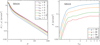 |
Fig. 1. Solid angle as a function of magnification and redshift for M0416. Left panel: cumulative solid angle corresponding to a magnification higher than a given value A(> μ) in the lens plane plotted as a function of magnification for a set of redshifts from 1 to 6 for the cluster M0416 at z = 0.397. The maximum solid angle corresponds to the 25 arcmin2 surveyed area in each cluster. Right panel: cumulative solid angle A(> μ) for μ = 10, 20, 50, and 100 in the lens plane as a function of the redshift of the lensed source for the cluster M0416. |
In Fig. 2 we show an overview of the entire sample. In the left panel we show the solid angle A(> μ) in the lens plane versus the magnification μ for all the clusters we used, where μ is conventionally computed for zs = 6. We note a large spread in A(μ), showing that the magnification depends on the cluster properties, mainly total mass and mass distribution (including member galaxies along critical lines, ongoing mergers, etc.). In the right panel we show the total solid angle obtained summing the magnification maps of the 11 clusters. For a magnification of μ = 10 we have ∼10 arcmin2 in the lens plane, or a total of less than 1 arcmin2 in the source plane. This implies that the probability of finding X-ray lensed sources at μ > 10 in our data is relatively low. These aspects are further explored in Sect. 7 when we discuss a possible extension of this work to current X-ray data archives and future missions.
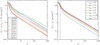 |
Fig. 2. Solid angle as a function of magnification and redshift for the 11 clusters. Left panel: solid angle A(> μ) in the lens plane for each of the 11 clusters as a function of μ(zs = 6). Right panel: cumulative solid angle A(> μ) in the lens plane for our entire sample for a source redshift from 1 to 6. The vertical dashed line shows the lower magnification limit μmax = 1.5 that defines the field of view we investigated. |
We also explored the correlation between the virial mass of the cluster computed at r200 and the high-magnification area in the lens plane. In Fig. 3 we show this relation for μ > 10 (assuming zs = 6 in this case as well). Using a simple linear function A(μ > 10, zs = 6) = a ⋅ (M200/1014 M⊙)+b to fit this relation and considering a 20% typical error for the solid angle, we find a = 0.08 ± 0.01 and b = −0.17 ± 0.02 (see the dashed line in Fig. 3). We remark that the effect of the intrinsic scatter (measured to be ∼0.2 dex, and probably associated with the details of the mass distribution) and the limited size of our sample do not allow a meaningful investigation of this relation, which would instead be a relevant property for the estimate of the total lensing power of the full cluster sample available in the Chandra archive.
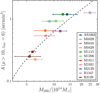 |
Fig. 3. Solid angle A(μ > 10) in the lens plane computed for z = 6, plotted against the virial mass computed within r200 from the weak-lensing measurements of Umetsu et al. (2018). Masses of M1311 and M2129 are based on X-ray scaling relations according to Liu et al. (2020a). The dashed line shows the best-fit linear relation A = 0.08 × (M200/1014 M⊙)−0.17 as a reference to appreciate the slope of the relation in our sample. |
4. X-ray emission from lensed sources identified in the optical
In this section we focus on the optically identified lensed sources that fall within a maximum field of view of 5 × 5 arcmin2 centered on the cluster X-ray center. Optically identified lensed sources belong to two different subsets. The first set includes all the sources with multiple images and is obtained from Caminha et al. (2019), Bergamini et al. (2019, 2021), and Vanzella et al. (2021). These are the counterparts used in their strong-lensing analysis. The second set consists of all the other sources with spectroscopic redshift higher than the cluster redshift, and therefore lensed at some level. In practice, we adopted conservative cuts corresponding to z > zcl + 0.1. In addition, we also set a lower limit on the expected magnification factor to avoid that it is dominated by nonlensed (μ ∼ 1) sources. Clearly, the magnification effect is maximized when we consider regions where the magnification is significantly higher than 1. However, the solid angle A(μ) for the entire sample decreases rapidly for low μ, as shown in Fig. 2 (right panel). We note that a threshold μmax > 3 or μmax > 2 would reduce the useful field of view in the lens plane by a factor ∼10 and ∼7, respectively. Because the statistics in our sample is limited, we therefore preferred to adopt a softer threshold μmax > 1.5 that reduces the useful field of view by less than a factor of 3 (see dashed vertical line in Fig. 2). By also including the low-magnification regime down to μmax ∼ 1.5, we obtained a statistically significant list of lensed sources for each cluster on the basis of the current imaging and spectroscopic analysis in the optical band, as we also verified a posteriori.
We note that the total solid angle in the source plane corresponding to the solid angle in the lens plane in which we searched for X-ray emission is measured with good approximation by ΣiAi/μi, where Ai is the area of a resolution element, μi is the maximum magnification at each position, and the sum is performed over all the positions where μmax > 1.5. This approximation does not account for the fraction of the field of view in the lens plane that is folded in the source plane. However, this fraction is negligible when compared to the variation in magnification associated with the redshift range of the sources, as we tested by comparing this approximation with the source and lens-plane mapping obtained with full ray-tracing at specific redshifts. Finally, we obtain a total of 61.9 arcmin2 in the source plane.
Our strategy consisted of three steps. Driven by the high-resolution HST images, first we visually inspected the X-ray images in the soft (0.5−2 keV) and hard (2−7 keV) bands separately to search for X-ray emission from single sources. Then, we performed aperture photometry at the source position and inspected the distribution of measured values in the soft and hard bands. Finally, we estimated the cumulative X-ray emission from the bulk of the optically identified lensed sources by stacking the X-ray data at the source positions.
4.1. Optically identified lensed sources: Visual inspection
First, we searched for X-ray emission from single sources by visual inspection. We proceeded in two steps: examining the original X-ray images, and then studying the residual images after subtracting background emission and the ICM foreground emission.
To obtain the residual images, we modeled the ICM component with two or more smooth ellipsoids in the Sherpa software. First, obvious unresolved X-ray point sources were removed from the images. The holes left in the images were filled with a Poissonian realization consistent with the surrounding signal. The cleaned image, largely dominated by the ICM, was fit with a combination of two elliptical β-models plus a constant background. A double β-model provides acceptable fits for most of the clusters in our sample. However, 4 out of 11 clusters, namely AS1063, M0416, M1206, and R1347, are undergoing a major merger process of multiple subhalos and required a more complex modeling. For these clusters, we considered four independent β-model components. For M0416 and R1347, where a bright cool core coexists within a disturbed morphology due to an ongoing major merger, we further added another component for the bright emission excess in the cool core. This process was applied separately to the soft- and hard-band images. Finally, the residual images were obtained by smoothing the original images with an FWHM of 0.5″ and then subtracting the best-fit models. Because the signal obtained as the difference of the two images is non-Gaussian, the residual images were not used for quantitative analysis, but were used only as support for the visual inspection to highlight possible candidate X-ray sources. Clearly, residual images are also a good resource to search for extended features in the ICM, such as sharp edges and cavities. However, we do not discuss this aspect here and refer to Donahue et al. (2016) for a detailed ICM morphological analysis of CLASH clusters.
Before performing the visual inspection, we fixed the size of the region we used for photometry, or extraction radius Rext (i.e., the circle within which we measured the emission of an unresolved source) according to the PSF at the source position. For multiple observations, the combined PSF was obtained by weighting each PSF map by the corresponding exposure map and exposure time. For simplicity, we ignored the departure of the shape of the PSF from circular because this aspect affects our analysis only little. We set the extraction radius Rext to the size of the PSF corresponding to a 90% enclosed energy fraction as computed with the task mkpsfmap within CIAO, setting a minimum value of 1.3 arcsec2. This choice was a good compromise between the need to maximize the encircled energy fraction and simultaneously keep the extraction region as small as possible to avoid the dilution of the signal by the high and structured foreground due to the ICM. This is relevant also considering that the cluster usually is not centered on the Chandra aim point, so that the PSF significantly degrades across the FOV. In addition, we manually adapted the shape of the source region in the few but relevant cases in which the lensed sources were significantly extended as a result of strong lensing. A case in which X-ray emission may come from single unresolved regions along a strong arc is expected (see Bayliss et al. 2020). We also had to slightly move or reduce the source region to avoid the few bright X-ray sources (mostly foreground galaxies and AGN) in the field. Finally, when optical counterparts belonged to the same family closer than the typical X-ray resolution, we merged the region of the nearby sources to obtain a single X-ray aperture photometry.
Our visual inspection consisted of searching for a distribution of pixels consistent with a PSF-like distribution on top of the background or foreground emission, using the experience gained in the investigation of deep fields such as the CDFS that have been performed by our group in the past. Although the identification of faint sources in extremely deep exposure is made with a high background, the main difference here is the strong foreground with a complex small-scale structure that makes the identification process significantly harder than in the field. The visual inspection provides us with a preliminary list of 20 X-ray source candidates either in the soft or in the hard band. Most of them are barely visible against the overwhelming ICM emission, but they are sometimes emphasized in the residual images. As described above, the residual images are very sensitive to irregularities in the ICM distribution, which can be associated with a plethora of features from infalling subhalos to edges, cold fronts, and cavities in the ICM. While all these features are extended, which is different from the unresolved emission expected from background sources, it may well happen that the combination of real ICM features and noise makes them compatible with the signal from unresolved sources. Clearly, mastering this aspect goes well beyond the goal of this work. To measure the flux of these sources, we adopted a simple aperture photometry. This method is certainly affected by Poissonian noise, but it does not depend on any other assumption. It also has the positive aspect of providing a simple and well-defined selection function that can be directly computed field by field. This aspect is crucial for the untargeted source detection and the measurement of the cumulative number counts, as shown in Sects. 5 and 6.
4.2. Optically identified lensed sources: Aperture photometry
We performed aperture photometry at the source position for the 20 source candidates that were visually selected. A critical aspect is the evaluation of the photometric error. To sample the local emission from the ICM, the background region for each source was determined as an outer annular region with a thickness of 2″, with the innermost annulus at 1 arcsec distance from the source region. The area occupied by the few bright X-ray sources (mostly foreground AGN) was masked out when the background was measured. However, X-ray bright spots were not masked because they might be associated with the intrinsic fluctuations of the ICM and must naturally be included in the noise affecting the aperture photometry. Finally, the 1σ error on the net counts was conservatively computed as  , where C is the value of the net counts and B is the value of the background or foreground counts rescaled to the source extraction region.
As expected, in several cases the photometric measurement is consistent with a null signal within one σ. Because the robustness of these sources is mostly based on a visible excess at the optical source position, we obtain a small but reliable list of X-ray emitting lensed sources when we apply a further filter on the S/N. The reference choice for the S/N threshold is S/N = 2 in at least one of the two bands, and this is used generally throughout the paper (see Rosati et al. 2002). Only 11 sources meet this criterion, including a few with 1.8 < S/N < 2, which were recovered on the basis of their convincing visual appearance. For each source we computed the energy flux as fX = S × ecf × Haimp/Hs, where S is the net count rate (the net count divided by the total exposure time in the field), ecf is the energy conversion factor, and Haimp and Hs are the values of the exposure map at the aim point and at the source position, respectively. In particular, Hs was averaged over the source extraction region. This was computed separately in the soft and hard band. For the ecf, we used the mean value of the two listed in Table 2, corresponding to spectral shapes with Γ = 1.4 and 1.8. The full range was accounted for as a systematic error on the fluxes and was summed in quadrature to the dominating statistical errors from aperture photometry. All the relevant information for the 11 X-ray emitter candidates are listed in Table 3. In Fig. 4 we show three examples of lensed X-ray emitting candidates, comparing the X-ray and the HST images, and highlighting the extraction regions Rext we used for aperture photometry. The first two panels show the two sources with the highest magnification values, and the third panel shows the pair of candidates in the field of R2129; they lie at the limit of our detection threshold.
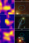 |
Fig. 4. Examples of identified X-ray counterparts of optically lensed sources. Left panels: residual X-ray images (soft band), and right panels: HST images. Contours are those used for aperture photometry in the X-ray bands. Top panels: source 23 in the FOV of M1115, with μ ∼ 74. Middle panels: source 46 in the FOV of AS1063, with μ ∼ 30. Bottom panels: sources 12, 13 (elongated region), and 73 (circular region) in the FOV of R2129, with μ ∼ 1.5, 1.5, and 1.9, respectively. |
X-ray emitting sources identified by visual inspection at the position of optically lensed sources.
We have five sources in two different fields that have one or more counterparts in addition to the counterpart that is identified as an X-ray emitter, labeled “(m)” in Table 3. Therefore we were immediately able to verifiy on the X-ray images whether the photometry at the position of the other counterparts was consistent with our detection. We find that in three cases the lack of detection in the other counterparts is still consistent within 1σ, while in the case of M0416−241 and M0416−208, we should have detected their counterparts with a signal of more than 3σ, but we obtained a null photometry at the corresponding positions. In addition, M0416−208 is very close to a cluster member (< 2″) that might easily contaminate its photometry. Therefore these two sources were not considered in our further analysis. The details of the confirmation of the multiple counterparts are given in the appendix.
The magnification distribution peaks at low values (∼2), and only two sources lie in the high-magnification regime (μ = 30 and 74). In Fig. 5 we show the distribution in the z − μ plane for the nine sources that were selected as reliable X-ray emitter candidates. Typical errors on the magnification are modest, about 10%, up to values μ ∼ 10, but they rapidly increase above μ ∼ 20 (see, e.g., Bergamini et al. 2021). Most of the detections are found in the low-magnification regions, and the probability of observing a highly magnified X-ray source among the optically lensed sources is very low.
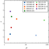 |
Fig. 5. Redshift and magnification of the sources in Table 3 identified by visual inspection after removing the two sources marked with the asterisk. The 1σ error on magnification is about 10% up to μ = 10, and it can reach a factor of 2 or higher for μ > 20. |
In Table 4 we list the rest frame delensed X-ray luminosity of the X-ray emitting sources listed in Table 3 except for the two that have been discarded. Luminosities are corrected for Galactic absorption but not for intrinsic absorption, therefore only a flux-luminosity conversion is used in each band, with a K-correction computed for an average spectral slope of Γ = 1.6. The uncertainty in the spectral shape is already accounted for in the error of the flux. In several cases, particularly in the hard band, we are able to only set a 1σ upper limit. Applying a crude classification in terms of X-ray luminosity, we find three sources (one of which includes two optical counterparts) consistent with being dominated by X-ray emission from star formation, with luminosities LX < 1042 erg s−1 in the soft or LX < 2 × 1042 erg s−1 in the total 0.5−10 keV band (AS1063−46, M0416−12, R2129−12 and 13, and barely M1115−23). The luminosities of the other six sources lie in the range 8 × 1042 − 5 × 1043 erg s−1 in the soft band, corresponding to moderate Seyfert-like galaxies. The only two sources with hard-band detection also appear to have significant absorption. The two sources in the high-magnification regime are instead consistent with being powered in the X-ray band by star formation. This is expected because at their delensed flux level (∼3 × 10⁻¹⁷ erg s−1 cm−2), the number density of star-forming galaxies is smaller by a factor of 3 than the number density of AGN. Overall, the few sources we identified so far show the typical mix of sources expected in this flux range. We did not attempt to further characterize these sources because the quality of the X-ray spectra is poor.
4.3. Optically identified lensed sources: Cumulative emission
We searched for additional signal from the bulk of the optically identified lensed sources. The distribution of aperture photometry for the entire sample of 837 source counterparts (after removing the 11 sources with identified X-ray emission in the previous step) is shown in Fig. 6. We note that the values on the negative and positive side of the photometry distribution are occasionally very high. These events are associated with a region of extremely high ICM emission, and the corresponding values have an extremely large error as well. However, some signal may be present close to ∼10 net counts in both bands, possibly associated with a subthreshold signal from the source population. Therefore we removed 47 anomalously high photometric values by performing a 3σ clipping and computed the stacked photometry (the sum of all the photometric values). We found no positive signal, and we are able to place only upper limits on the average observed flux of 4 × 10⁻¹⁶ erg s−1 cm−2 and 1.8 × 10⁻¹⁵ erg s−1 cm−2 in the soft and hard bands, respectively, at a 3σ confidence level. To better appreciate this result, in Fig. 7 we show the stacked X-ray images of all the sources in the soft and hard band. We also computed the cumulative photometry on the stacked image in an aperture of 3 arcsec, finding −218 ± 155 and −90 ± 128 net counts in the soft and hard bands, respectively. These values are consistent with what we previously found by summing the aperture photometry at each source position, and we confirm that the cumulative X-ray emission from the bulk of the optically identified lensed sources is well below our detection limits.
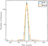 |
Fig. 6. Histogram of aperture-photometry values in the soft and hard bands (cyan and orange histogram, respectively) for the 837 optically lensed sources in the 11 cluster fields after removing the visually identified sources listed in Table 3. The thick solid lines show the normalized best-fit Gaussian functions. |
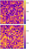 |
Fig. 7. Stacked X-ray image of all the optically identified lensed sources after removing the 11 X-ray detected sources and clipping the extreme photometry values as described in the text. Images are 10″ across, and the color scale indicates net counts. Upper and lower panels: soft and hard bands, respectively. The white circle marks the 3 arcsec aperture we used for photometry in the stacked images. |
5. Untargeted search for X-ray sources in the high-magnification region
The targeted search for X-ray emission from lensed sources in the field of our CLASH clusters provided us with only 11 candidates drawn from the lensed sources previously identified in the optical band. Clearly, we still have X-ray lensed sources that were not previously identified in the optical. Some may be associated with optical counterparts that have no redshift, and in some other cases, with sources with high fX/fopt; in both cases they are potential X-ray lensed source candidates. Therefore we proceeded with the untargeted detection of sources in the X-ray images. Although the ICM makes the X-ray detection process quite different and much harder than in the field, we did not develop an ad hoc algorithm for the ICM emission and its spatial variations. A proper and self-consistent modeling of the ICM would require an effort well beyond the possibilities of current X-ray imaging analyses. Instead, we adopted a standard procedure that was validated and calibrated a posteriori with imaging simulations.
5.1. X-ray lensed source candidates identified with wavdetect
The X-ray source detection was performed using the wavdetect tool (Freeman et al. 2002) on the soft (0.5−2 keV), hard (2−7 keV), and total (0.5−7 keV) band images. The wavelet scales were set as 1, 2, 4, 8, 16, and 32, and the false-positive probability threshold was set to 10−5. This high threshold (compared to the 10−6 − 10−7 range that is commonly used for robust detection) does not correspond to any predictable contamination fraction because of the strong and rapidly varying foreground, and it is expected to provide a generous number of source candidates. A source list obtained with this strategy therefore needs to be further refined with much tighter criteria. We merged the source lists obtained independently from the soft, hard, and full bands to include all the source candidates that were detected in at least one of the three bands. The threshold for merging sources is a distance smaller than Rext. A few cases of double detections that were not resolved by our matching criteria3 were fixed after visual inspection. The direct output of the wavdetect algorithm provides us with 388 source candidates in the 11 cluster fields. Then, we carefully filtered this list by applying a series of steps.
First, we verified whether we recovered the 11 previously identified sources by matching the wavdetect X-ray position to the optical position by applying a criterion based on the distance. Matched sources are those for which the distance is smaller than Rext. Only 3 out of the 11 sources (AS1063−31, M0416−208, and M1206−18) were recovered. This implies that 8 sources are below the wavdetect detection threshold and were identified only by the combination of a positive aperture photometry and the spatial overlapping with a magnified source. This indicates that the combination of a high wavdetect selection algorithm with threshold parameter 10−5 and the S/N > 2 condition may not give completeness ∼1, particularly close to the S/N > 2 threshold and in the regions that are deeply embedded in the strong ICM emission of the cluster core. This aspect was considered with simulations as explained in the next section.
In the second step, we searched in the list of published redshifts from the CLASH-VLT survey (Biviano et al. 2013; Monna et al. 2017; Caminha et al. 2016, 2019; Balestra et al. 2016; Karman et al. 2017; Bergamini et al. 2019) for optical counterparts with a redshift lower than the cluster redshift (or, more accurately, zs < zcl + 0.1). In this way, we identified 24 foreground sources with X-ray emission that were removed from the list of X-ray lensed source candidates.
Because we chose from the beginning to focus on the solid angle corresponding to μmax > 1.5 to avoid a large contribution from the much larger field of view with low magnification, in the third step we also removed the source candidates that were found at μmax < 1.5. We remark that the choice of using the maximum magnification is just a convention, and another choice (e.g., using the magnification at zs = 6) would not affect our results because this step is needed uniquely to restrict our field of view to the most relevant regions for our purposes. We find that 140 source candidates correspond to positions with μmax < 1.5. After this step, 221 sources were left.
In the fourth step, we performed aperture photometry. Before this, we visually inspected the extraction regions of source and background, defined as described in Sect. 4. In some cases we manually adjusted Rext, and more often, the size of the background regions, particularly when these extended across areas in which the ICM emission varies significantly. This process mostly affects the few sources that are deeply embedded in the core of the cluster, where the small-scale fluctuations of the ICM inevitably introduce large uncertainties. Therefore we also considered the background and foreground estimated from our modeling of the ICM emission in the soft and hard band, which allowed us to measure it directly in the source region, under the assumption that the ICM is well represented by the smooth surface-brightness fit. We identified several sources for which the two photometry methods provide significantly different results, showing that ICM fluctuations heavily contaminate the sources candidates obtained with wavdetect. All these cases are located in the core or slightly outside the core. Therefore we conservatively included only the sources for which the two methods provided consistent photometry. We inspected the removed sources to verify whether some reliable source candidate might have been discarded in this step, but we found none. Finally, we selected all the sources with S/N > 2 in the soft or in the hard band.
This series of steps provided us with a list of 80 candidate X-ray lensed sources with a well-defined selection criterion in the X-ray band. The two methods for performing aperture photometry (sampling the background or foreground from the surrounding regions, or modeling with a global fit of the surface brightness) are shown to be consistent with each other within the statistical errors for the list of 80 source candidates in Fig. 8. At this point, we applied a fifth and last selection step by investigating the source candidates with visual inspection of the corresponding HST and Subaru images. This step allowed us to identify the cases in which the X-ray emission is associated with an obvious foreground object at low redshift or with a cluster member. This step is complementary to the removal of the sources with measured redshift zs < zcl + 0.1 because not all the foreground sources have a measured redshift. We removed 14 sources in this last step. All the X-ray sources without redshift that we kept in our sample are consistent with being in the background of the cluster. However, we acknowledge that some of them may still be in the foreground, and therefore our final source list is an upper limit to the number of X-ray sources that are lensed by the clusters with μ > 1.5.
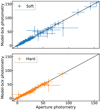 |
Fig. 8. Comparison of the aperture photometry values obtained with modeled or directly sampled background and foreground for the soft band (upper panel) and hard band (lower panel). The solid line shows the x = y relation. |
In addition, we took advantage of the comparison with HST and Subaru images to refine the source position, particularly for the sources that lie very close to the critical lines. Only one source (R1347−7) has a rapidly changing magnification within the X-ray position error, therefore we used the position of the HST counterpart to improve the accuracy of the magnification. All the other sources lie at positions far from the critical lines and therefore depend smoothly on the magnification of the centroid position. In the low-magnification regime (μ < 6) an uncertainty of 1″ in position corresponds to an uncertainty of ∼5% on μ, and therefore we assumed this value as an upper limit of the uncertainty on the magnification associated with the position. However, the lack of a redshift for most of the X-ray lensed source candidates implies an additional uncertainty on the magnification. Because it is not feasible to extract the redshift from the sparse optical information we have for our X-ray lensed source candidates, we chose an approximation based on the actual redshift distribution of X-ray sources found in the CDFS (see Fig. 9 in Luo et al. 2017). We considered star-forming galaxies and the AGNs together because we lack a source classification in the redshift interval 0.5 < z < 4 in which most of the lensed X-ray sources are expected in our fields. The probability for a source in the CDFS to be in a given redshift bin is approximated by the probability distribution shown in Table 5. When we consider only sources in a flux range comparable to our source list (10−16 − 10−14 erg s−1 cm−2 and 10−15 − 10−13.5 erg s−1 cm−2 in the soft and hard bands, respectively), we find a very similar distribution, with differences smaller than 10% in every bin. Therefore the probability of any source in these flux intervals to have a given redshift is approximately described by the stepwise normalized function p(z) shown in Table 5. By weighting the μ(z) at each position in the FOV by the average redshift distribution of CDFS sources, we obtain the best guess for the magnification associated with each source simply as μw ≡ Σiμ(zi)×p(zi) (where zi are the mid points of the redshift bins in the first column of Table 5).
Fractional distribution in bins of redshift for the sources of the CDFS (normalized total number of sources in the range 0.5 < z < 4).
The properties of the final sample of 66 X-ray selected sources, including observed flux and weighted magnification, are shown in Table 6. In Fig. 9 we show the histogram distribution of the lensed and delensed fluxes in the soft and hard band. The lensing effect consists of a shift of about a factor of 2 in sensitivity for the bulk of the sources in both bands. However, the sensitivity of each field is lower on average than the sensitivity of a blank field with the same Chandra exposure because of the foreground ICM emission. A similar result can be seen in the scatter plots of observed flux versus magnification in Fig. 10. Only two sources in the soft band occupy the lower right part of the plot, where the combination of low flux and magnification brings the delensed flux range below the 10−16 erg s−1 cm−2 limit, marked by the solid black line. None of our sources is identified below 10−17 erg s−1 cm−2 (dashed blackline), which is about three times higher than the flux limit of the CDFS in the soft band. In the hard band (lower panel) the solid line marks the delensed flux limit 10−15 erg s−1 cm−2, which is 1.5 orders of magnitude higher than the hard-band flux limit in the CDFS. Only two sources (with low magnifications) are observed below this limit. Clearly, these detection limits are significantly affected by the ICM emission, an important effect that we better quantify in the next two subsections.
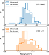 |
Fig. 9. Distribution of observed and delensed fluxes in the soft (upper panel) and hard (lower panel) bands for the sources detected with our algorithm (Table 6) plus sources with optical counterpart (as in Table 3). Only sources with S/N ≥ 2 in each band are shown. |
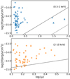 |
Fig. 10. Scatter plot of the soft (top panel) and hard (bottom panel) observed flux vs. the weighted magnification. Top panel: the region below the solid and dashed black lines corresponds to delensed fluxes below 10−16 and 10−17 erg s−1 cm−2, respectively. Bottom panel: the region below the black line corresponds to delensed fluxes below 10−15 erg s−1 cm−2. Sources marked with circles are X-ray selected, and triangles correspond to sources identified as X-ray counterparts of optically lensed sources (listed in Table 3). Only sources with S/N ≥ 2 in each band are shown. |
5.2. Completeness and contamination maps with imaging simulations
Before computing the flux limit corresponding to our selection threshold S/N > 2, we evaluated the completeness, defined as the ratio of the recovered over the total sources above the detection threshold. This step would not be necessary if the detection algorithm, in our case wavdetect, were able to identify all the sources down to S/N = 2 or below. Clearly, a solution is to raise the selection threshold up to a level above which the detection algorithm is complete, but this would result in a significantly lower number of selected sources and therefore a poor statistics. Another strategy is to refine the detection algorithm at the point of reaching completeness at the desired selection threshold, but this would imply a significant amount of work, and, unavoidably, an increasing contamination from spurious sources. Clearly, the best solution is a compromise, with a reasonably low threshold (S/N > 2 is the same used in the CDFS, see Rosati et al. 2002), and an accurate estimate of the completeness (or recovery rate) in order to be able to apply this correction a posteriori.
To compute the completeness correction, we used a direct approach using imaging simulations. As a first step, we obtained background- and foreground-only images in the soft and hard bands by removing a circle defined by Rext around each source identified in the first step with wavdetect, and filling it with a Poisson realization consistent with the surrounding background and foreground. Then we simulated point sources distributed randomly in our 5 × 5 arcmin2 field of view centered on the cluster center, distributing them across the pixels according to a PSF consistent with that expected at each position in the real data. For simplicity, instead of generating the 2D PSF by ray-tracing for each position in the image, we used a 1D Gaussian PSF, which is a good approximation to the real composite PSF except in the outskirts of the field, which are excluded by our selection. For each field of view and a given value of input net counts, we simulated ∼1000 images with only ten sources each to avoid overcrowding. Because of the low density of X-ray sources in our fields and the high angular resolution of Chandra, we can ignore confusion effects and correlation. The input count for each source ranged from 5 to 100, with a step of 5 counts. Simulated images were then analyzed by running wavdetect with the same threshold parameters of 10−5 as we used on the real data. Then we matched the position of the detected sources with the input positions, adopting a matching radius proportional to Rext. We considered only sources with a measured aperture photometry corresponding to S/N > 2, following the same selection strategy we used for the real data. To derive the net counts, we applied aperture photometry using the background and foreground as modeled by our fit of the soft and hard surface brightness.
Finally, for each simulation, we collected three types of sources: Recovered, lost, and spurious sources as a function of the input net counts and the position in the image. The completeness, or recovery rate at S/N > 2, is defined as the ratio of recovered to simulated sources for a given range of input net counts. The completeness maps were obtained in the following way. For each pixel in the image, we computed the average recovery rate within a circle of r = 15 pixels as a function of the input net counts C. This fraction depends in a nontrivial way on the PSF shape and the background and foreground level in a given region of the image. In particular, we note that in most of the cases, the aim point of a single observation does not coincide with the cluster center, a choice that is often adopted by the observers to avoid the CCD gaps in the core regions. While this choice is optimal for the ICM science, it is not optimal for the search for unresolved sources close to the critical lines because the PSF quality rapidly decreases at off-axis angles larger than 3 arcmin. As a result, the best PSF of the combined image is not obtained at the center of the cluster. This aspect, as we discuss below, significantly limits the search for X-ray lensed sources in Chandra images, as opposed to future X-ray missions that aim at ∼1 arcsec resolution on a large field of view.
Based on the imaging simulations, we obtained 20 completeness maps, corresponding to 20 different values for the input counts, for each cluster in the soft and hard bands (for a total of 440 completeness maps). Some of them are shown in Fig. 11 for some representative values of net input counts. We note that completeness is rather high (> 90%, corresponding to bright yellow) for a large part of the FOV considered here (5 arcmin by side centered on the cluster). A significant fraction of the field of view has a completeness of ∼0.5, while only the central regions, swamped by the core emission, are highly incomplete (up to a factor of 10). As previously discussed, the completeness maps are not symmetrical with respect to the cluster center because of the offset of the minimum PSF (marked in Fig. 11 with crosses) with respect to the cluster, and this significantly affects the capability of detecting faint sources with our algorithm. Most importantly, these maps highlight a strong difference between the sensitivity and the magnification in the most interesting regions close to the critical lines. This aspect is further discussed in Sect. 7. The completeness maps were used to weight each source by the probability of detecting it according to its position in the field and its measured net counts. This weight is assumed to be the inverse of the completeness value.
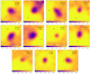 |
Fig. 11. Completeness maps in the 0.5−2 keV band for all the sources with S/N > 2 detected with wavdetect in the 11 cluster fields. The color code indicates the completeness or recovery rate at a given input net counts N, as shown in the color bar, in the 0.5−2 keV band. The maps are 5′ across and are smoothed with a Gaussian FWHM of 10″. The black crosses mark the position of minimum PSF in each field, resulting from the overlapping of several exposures with different aim points. The low recovery rates in cluster centers and in the corners of the field of view are due to the strong ICM emission and the increase in PSF size, respectively. |
Focusing on the spurious sources, we directly obtained their distribution in each field in the soft and hard bands by computing their average number at each position for a given value of the observed net counts. The expected number of spurious sources with apparent S/N > 2 per field is about 0.10−0.15 in the soft and 0.10−0.20 in the hard band, most of which are concentrated in the cluster core, as expected. The cumulative number of spurious sources expected per field with measured net counts above a given value in the soft and hard bands is shown in Fig. 12. We immediately note that the total expected number of spurious sources at S/N > 2 for the entire survey (the sum of the 11 fields) is about 2−3 summed in the soft and hard bands. Considering that we also applied an accurate visual inspection that led to the removal of several unreliable sources in the core region, we can reasonably expect a low fraction of spurious sources, distributed in counts according to our simulation as shown in Fig. 13. The corresponding fraction is computed as the ratio of the average number of spurious sources found with simulation in the entire survey, divided by the detected sources in each count bin. From this distribution, we can associate with each source that is detected with a given number of counts in each band the probability of being a real source equal to one minus the spurious fraction. The fraction of spurious sources drops in the lowest count bin instead of being maximum, as expected. The reason is that the spurious sources with observed counts between 5 and 20 are excluded by the S/N > 2 criterion.
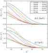 |
Fig. 12. Cumulative number of spurious sources N expected per field with measured net counts below C for each cluster in the soft (upper panel) and hard (lower panel) bands. |
 |
Fig. 13. Ratio of spurious sources over detected sources in the entire survey in bins of observed net counts in the soft (top panel) and hard (bottom panel) bands. |
5.3. Flux-limit maps and sky coverage
Finally, we computed the sky coverage as a function of the source flux in the soft and hard band separately. The sky coverage is defined as the total solid angle in our survey where a source of a given flux can be detected with our selection criteria. We obtained a flux-limit map by computing the flux corresponding to our selection threshold S/N > 2 in each point of our image. Technically, the flux limit is computed on the basis of the X-ray images cleaned from the unresolved sources that we also used for the imaging simulations. From the condition  , we computed at each position the minimum net counts Cmin that satisfied our selection criterion. We recall that B represents the counts expected within Rext contributed by the background and the foreground (ICM). Then we considered the net count rate corrected for vignetting and multiplied it by the average conversion factor, as explained in Sect. 4.2, to obtain the flux limit at each position. The flux limit therefore depends on the background and foreground and on the size of the extraction region in which the aperture photometry is performed, both of which strongly depend on the position of the source in the image. The total solid angle of our survey as a function of the flux fX was obtained by computing the total solid angle whose flux limit flim is below fX. The sky coverage corresponding to a given flux is therefore simply the solid angle satisfying both μmax > 1.5 and flim < fX.
We can plot the sky coverage measured on the sky (lens plane) or delensed, that is, obtained by mapping the solid angle in the lens plane back to the source plane and weighting the source-plane maps by the average redshift distribution. Here we approximated this step by weighting each pixel by  . As described above, weighting the solid angle by the inverse of the magnification value in each position does not take into account the regions in the lens plane that correspond to the same region in the source plane. We evaluated the effect of this approximation by comparing the average field magnification obtained with the full ray-tracing for a specific redshift (see, e.g., Meneghetti et al. 2008, 2010; Plazas et al. 2019) to that obtained with the simple inversion, and found that the differences are in the range 1%−3%, with a maximum of 6% in the case of R1347. Because the uncertainties associated with the unknown redshift of the sources are significantly larger, we conclude that our strategy to compute the solid angle in the source plane by dividing the lens plane value by μw is acceptable.
The two sky coverage functions for the entire survey (11 CLASH fields) as a function of the observed (lensed) flux are shown in Fig. 14 with dashed lines in the soft and hard band. The maximum solid angle in the lens plane, defined by the condition μmax > 1.5 (marked with a horizontal dashed line), is reached at ∼10−15 and ∼4 × 10⁻¹⁵ erg s−1 cm−2 in the soft and hard bands, respectively. The survey limits, conventionally defined by a sky coverage as small as 0.1 arcmin2, is reached at 10−16 and 3.5 × 10⁻¹⁶ erg s−1 cm−2 in the soft and hard bands, respectively.
 |
Fig. 14. Sky coverage as a function of flux for the 11 CLASH cluster fields. The thick solid curve shows the sky coverage in the source plane as a function of the de-lensed flux in the soft (left panel) and hard (right panel) bands. The thick dotted curve instead shows the same sky coverage in the source plane, but as a function of the observed flux. The sky coverage in the source plane was used to compute the delensed log N–log S. The sky coverage in the lens plane is also shown as a function of the delensed flux (continuous curve) and of the observed flux (thin dotted curve). The horizontal dashed line indicates the total solid angle, by the criterion μmax > 1.5. The black curve shows the sky coverage of the 7 Ms CDFS survey in the corresponding energy ranges (Luo et al. 2017). The hard-band flux limits in Luo et al. (2017) given in 2−7 keV are converted into 2−10 keV by assuming Γ = 1.8. |
In Fig. 14 we also plot the lens- and source-plane sky coverage as a function of the delensed flux (solid lines). The sky coverage in the lens-plane as a function of the delensed flux is significantly deeper. However, a more useful quantity is the sky coverage in the source plane versus the delensed flux. When we compare this to the same quantity plotted versus the observed flux, the effect resulting from the combination of magnification and source dilution of gravitational lensing is immediately clear. The net result is that the lens allows us to reach deeper on average by only a factor of two, as we already noted when we compared the distribution of observed and delensed fluxes. The same behavior is observed in the soft and hard bands. Unfortunately, when combined with the flattening of the soft and hard bands log N–log S at the faint end, this implies that an increase of a factor of ∼2 in depth corresponds to a limited increase in the number of faint sources.
To compute the log N–log S, we used the source-plane sky coverage either matching the de-lensed flux or the observed flux to the corresponding flux of each source, and we plot the cumulative source number as a function of the delensed flux for a direct comparison with the log N–log S measured in blank fields or modeled.
6. logN–logS of X-ray lensed sources in CLASH fields
6.1. Expected logN–logS
The deepest X-ray field to date (and in the future, until a new X-ray mission with arcsec resolution will be operational) is provided by the CDFS (Giacconi et al. 2001; Rosati et al. 2002; Luo et al. 2017), which has reached the unparalleled depth of 7 Ms. From the number counts published in Luo et al. (2017, see their Fig. 31), we note that the density of X-ray sources in the sky is rather low. We considered the delensed flux of ∼10−16 and ∼3 × 10⁻¹⁶ erg s−1 cm−2 in the soft and hard bands, respectively, that in our survey both corresponds to ∼1 arcmin2. In both cases the expected number of sources is slightly higher than one, implying that the CLASH survey runs out of sources below these fluxes.
However, we cannot directly compare our results with the full number counts as measured in the fields of deep or medium-deep surveys such as CDFS or COSMOS. We have reported the number counts of lensed sources only, which implies that we ignored all the nonlensed foreground sources with zs < zcl + 0.1. This choice was adopted to focus on lensed sources and avoid being dominated by unlensed sources as in blank fields. For a proper comparison, we therefore need to correct the expected log N–log S by removing the sources with zs < zcl + 0.1. To this aim, we used mock catalogs and tools4 based on the XRB model by Gilli et al. (2007) (see also Hasinger et al. 2005), which includes an exponential decline in the AGN space density at redshifts above z = 2.7 to cope with the results from wide-area surveys (e.g., SDSS Richards et al. 2006; Fan 2006). Because the Gilli et al. (2007) model includes only AGN, we added the steep galaxy number counts as measured by Luo et al. (2017) in the CDFS. However, normal (star-forming) galaxies are relevant only at fluxes well below 10−16 erg s−1 cm−2. This model provides cumulative number counts that agree with those measured in the SDSSJ1030 (Nanni et al. 2020) or the XBootes (Masini et al. 2020) fields and are slightly higher than those in the COSMOS field (Civano et al. 2016). The predictions are brought into good agreement with the AGN log N–log S in the CDFS when the normalization is reduced by a factor ∼0.8 in both bands. This is expected because of the already noted lower normalization of the cumulative number counts in the CDFS with respect to other deep fields (see, e.g., Fig. 7 in Liu et al. 2020b). Considering the uncertainties on the log N–log S, also associated with the actual source flux (for which an average spectral shape is assumed that is not representative of the wide distribution in intrinsic absorption), we decided to focus on the predictions from Gilli et al. (2007).
In the model by Gilli et al. (2007), the dependence on redshift is built in on the basis of the luminosity function of AGN as implemented in the model. This allows us to immediately compute the expected log N–log S only for sources with zs > zcl + 0.1 in each field. Because the redshift cut is different in each field, we summed the expected log N–log S in each field using a weight proportional to the total solid angle considered in our study (defined by the condition μmax > 1.5. The expected cumulative number counts after removing the foreground X-ray sources are plotted in Fig. 15. As expected, the decrease has a modest effect at the low-flux end, but it starts to be more evident at fluxes S > 10−14 erg s−1 cm−2.
 |
Fig. 15. Effects of the cuts in redshift for zs < zcl + 0.1 on the expected log N–log S of lensed X-ray sources in the soft (upper panel) and hard (lower panel) bands. The upper red lines show the total number counts from the model by Gilli et al. (2007), and the lower blue lines show the number counts expected for the lensed sources (zs < zcl + 0.1) on the basis of Gilli et al. (2007). The shaded areas are the CDFS number counts from Luo et al. (2017). The hard-band flux limits in Luo et al. (2017) given in 2−7 keV are converted into 2−10 keV by assuming Γ = 1.8. The predictions from Gilli et al. (2007) are multiplied by a factor of 0.8 to be consistent with the CDFS results. |
6.2. Cumulative number counts
The final list of sources we considered was obtained by adding the sources in Table 3 (excluding the two flagged with the asterisk) to the X-ray sources detected with wavdetect listed in Table 6. Therefore we considered a total of 68 sources. Among these we selected for each band those that satisfied S/N > 2, finding 55 sources in the soft band and 56 in the hard band. The cumulative number counts per solid angle were obtained by summing all the sources above a given flux, where each source was multiplied by three weights: by the inverse of sky coverage (computed at the corresponding source flux), the inverse of the completeness (which depends on the source position and source net counts), and the probability of not being spurious (which depends on the net counts). In a blank field (i.e., in absence of lensing), observed and intrinsic fluxes are the same, and therefore we have
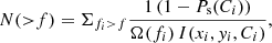
where Ω(fi) = ΣjAj(flim < fi, μmax > 1.5) is the sky coverage corresponding to the flux of the ith source, I(xi, yi, Ci) is the completeness at the source position and for the net counts Ci measured for that source, and Ps(Ci) is the probability of being a spurious source. As previously discussed, the factor 1/Ω(fi) is the weight to obtain the contribution of a given source to the source number density in the assumption of perfect detection (all the sources with intrinsic S/N > 2 are detected), while the factor 1/I(xi, yi, Ci) provides the correction due to the probability of detecting this specific source with a given detection algorithm. The factor (1 − Ps(Ci)) instead provides the small correction due to the probability of including spurious sources in the sample, and it only depends on the measured net counts Ci.
The additional complication in our survey is that in order to measure the true number counts (i.e., those that would be measured without the lensing cluster), we need to delens the observed fluxes and delens the sky coverage corresponding to a given observed flux. Therefore we define fi, dl = fi/μ, and Ωdl(fi, dl) = ΣjAj(flim, dl < fi, dl, μmax > 1.5)/μj, where flim, dl is the delensed flux limit. An equivalent quantity can be obtained using the observed flux and matching it to the observed flux of each source, given that the log N–log S is plotted against the delensed flux. The two approaches are not identical, but are expected to provide consistent results. We verified that the two log N–log S obtained by matching the delensed and the observed fluxes have negligible differences. Therefore we can obtain the delensed (or source plane) number counts as
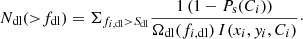
The delensed number counts in the soft and hard bands are shown in the left panels of Fig. 16. The 1σ uncertainty includes the Poissonian error on the source number and the error on the flux, obtained as the quadratic sum of the Poissonian error on the net counts and the uncertainty in the conversion factor. We note that the uncertainty in the cumulative number counts (shown as the shaded area) is dominated by the source statistics for bright sources, and as a consequence, it decreases with flux. On the other hand, at the faint end it is dominated by the error on the fluxes, and therefore it increases with decreasing flux. The uncertainty on the magnification, which would add another 10% to be summed in quadrature, has not been included here. When we compare our measurements to the expected log N–log S from Gilli et al. (2007) plus the contribution from star forming galaxies as in Luo et al. (2017) (shown with a solid thin line), we find a good agreement within the 1σ uncertainty, although the CLASH fields log N–log S shows an excess of approximately 20% where the discrepancy is maximum, at about 3 × 10⁻¹⁶ and 10−15 erg s−1 cm−2 in the soft and hard bands, respectively, and an average excess of ∼10% in both bands over the entire flux range. We note that differences of ∼10%−20% associated with cosmic variance have been observed in the deepest X-ray surveys such as CDFS, CDFN, and COSMOS. In a recent paper, the results from the XMM-RM survey have been compared with the CDFS and XMM-COSMOS number counts, and a substantial agreement was found except for a discrepancy of a factor 1.5 between the CDFS and the other surveys (see Fig. 7 in Liu et al. 2020b) in a relatively bright flux range. In general, a thorough discussion of the fluctuations in the normalization of the log N–log S due to cosmic variance has not been performed in the literature so far, and it is expected to be superseded by a detailed account of the distribution of AGN and star forming galaxies in redshift based on the increasing availability of complete multiwavelength surveys. Considering that the mild excess found in our measurements is well within the 1σ uncertainty and that our source selection may have included a few foreground sources because we lack redshift information, we do not regard this excess as significant. As a final point, we recall that the delensed fluxes (for single sources and for the flux-limit maps) were obtained assuming a representative redshift distribution derived from the complete CDFS survey. The actual redshift distribution of our selected sources may be different from the assumed one, causing a miscalibration of the average magnification effect. To summarize, considering the assumptions we adopted, we find a reasonable agreement of our results with the expectations.
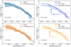 |
Fig. 16. Number counts of sources detected in the CLASH fields as a function of flux. Left panels: cumulative number counts of the lensed sources in the soft band (upper left) and hard band (lower left). The number counts are compared with the prediction by the model of Gilli et al. (2007) after removing the foreground sources. Right panels: effects of the flux magnification and source dilution shown separately in the soft band (upper right) and hard band (lower right). |
To better appreciate our results, we separately show the effect of flux magnification and source dilution as discussed in the optical band in Broadhurst et al. (1995) and in the X-ray band in Refregier & Loeb (1996). In a very simplified but useful scheme, we can assume a power-law behavior, with dN/df ∝ S−α − 1, and therefore N(> f)∝f−α. We assume that we observe a reasonably large region with constant magnification μ, then we can express the combined effect of the flux magnification and source dilution by writing the real cumulative number counts as a function of the observed ones as  . The delensed (intrinsic) and observed number counts would look similar when α ∼ 1. This is the approximated value for the slope in the considered flux range. We show in the right panels of Fig. 16 the two effects at play in the soft and hard bands. The thickest line is the directly observed log N–log S, obtained by plotting the cumulative number counts as a function of the observed flux and weighting by the corresponding solid angle in the lens plane. The medium-thick line is obtained by delensing the observed fluxes. This step is clearly roughly equivalent to a rigid shift toward the faint end. Finally, the thin line is the actual log N–log S, obtained by plotting the observed cumulative number counts as a function of the delensed fluxes weighting by the corresponding solid angle in the source plane. Again, this step is roughly equivalent to a rigid shift in the vertical direction. As previously shown, because the slope in both bands is close to α = 1, the two effects almost cancel out, and the net results is a shift along the relation toward the faint end, therefore a higher depth than in the observed flux.
The increased depth is the most relevant effect we searched for because a significant shift toward the faint end would allow us to explore the deep X-ray sky through the lensing effect of the clusters. Unfortunately, we note that the increase in depth is limited, and it is dominated by very few sources with high magnification or with low intrinsic flux. The faintest delensed flux in our survey is 1.4 and 1.6 dex higher than the faint end of the CDFS in the soft and hard band, respectively. Therefore we find that the gain in sensitivity caused by the intervening clusters due to the combined effect of the small solid angle at high magnification and of the strong diffuse X-ray emission from the ICM is a factor of ∼2 compared to blank fields with the same exposure. The implications of our study for the future use of massive clusters as cosmic telescopes in X-ray extragalactic surveys is discussed in the next section.
7. Perspective for future studies
Our results show that the combination of low number statistics for X-ray sources, the small solid angle associated with high magnification, and the overwhelming foreground due to the diffuse ICM emission significantly weaken the power of cosmic telescopes in the X-ray band. In particular, out of 11 massive clusters with exquisite optical data, we were able to identify only 3 X-ray sources that are magnified by more than a factor of 10. As a result, the delensed cumulative number counts of the X-ray lensed sources is far from approaching the flux limit of the deepest X-ray surveys: it reaches only ∼10−16 erg s−1 cm−2 in the soft band and ∼5 × 10⁻¹⁶ erg s−1 cm−2 in the hard band. The question now is whether we can develop a strategy on the basis of the current results to probe the X-ray sky population at fainter fluxes using massive clusters as cosmic telescopes.
On one hand, it is always convenient to determine whether highly magnified sources identified in the optical band are also X-ray emitters. The discovery of a bright, rare, high-redshift, highly magnified X-ray source, possibly with multiple images (as in the few known Einstein crosses associated with multiply lensed bright quasars) would be relevant not only to studying the spectral properties of a source that would otherwise have been weak, but also for the possibility of monitoring its flux variations, and with an accurate mass model of the lens, performing cosmological test as in the case of SN Refsdal (Kelly et al. 2015; Grillo et al. 2020). Intrinsically bright X-ray sources offer the advantage of being variable on short timescales, potentially offering a very efficient cosmological test. For this reason, it is always convenient to investigate the X-ray images of massive clusters that have been observed with deep optical data (the combination of HST and MUSE has been shown to be optimal for these studies) in search of such an object. However, this occurrence is expected to be very rare.
On the other hand, the systematic search for lensed sources to reach fainter X-ray sources has been shown to be difficult. Clusters of galaxies are not transparent in the X-ray, and the solid angle associated with high magnification typically is low. Together with the low number density per solid angle of X-ray background sources, this implies that the trade-off between the probability of finding X-ray sources is very close to a critical line, and the capability of identifying unresolved sources in the midst of the bright ICM emission is quite unfavorable. This discrepance is visualized in Fig. 17, where we show the flux-limit maps in the field of AS1063 for the observed and the delensed fluxes. Most the field reaches a delensed flux level slightly below the observed flux limit (about a factor of two), while in only a tiny region corresponding to the cluster critical lines does the magnification have a significant effect and overcomes the ICM bright emission.
 |
Fig. 17. Flux limit corresponding to the selection criterion S/N > 2 in the soft band for the AS1063 field. The observed flux limit is shown in the left panel, and the delensed flux limit is shown in the right panel. The images are 5′ across and are smoothed with an FWHM of 3″. |
We can better illustrate and quantify this trade-off by computing the maximum magnification at each position in our images and the decrease in sensitivity with respect to the field. The loss in sensitivity here is computed, consistently with our method, as the ratio of flux Slim corresponding to an S/N > 2 in a given position, divided by the minimum detectable flux in the same X-ray field Sfield, far from the ICM emission. The latter value is a reasonable proxy for the flux limit that we would have in the same observation if the ICM emission were not present (i.e., the sensitivity corresponding to the best PSF and the lowest background and foreground for a given observation). We also convolved the map by the completeness (this only applies to the wavdetect detection algorithm and is therefore valid for a standard approach of source detection). The two effects compete directly, so that the comparison of the values of μmax and the ratio Slim/Sfield indicates the regime in which the magnification exceeds the loss in sensitivity. In Fig. 18 we show the Gain, defined as the ratio μmax/(Slim/Sfield), in the soft band in the field of AS1063. We find that the solid angle where the magnification exceeds the loss in sensitivity (Gain > 1) is limited to a very small area, is dominated by values slightly higher than unity, and clearly peaks where the critical lines are. This visualizes the modest efficiency in using massive clusters as cosmic telescopes in the X-ray band. To be more quantitative, in Fig. 19 we plot the cumulative solid angle in each field where the gain is higher than a given value. The solid angle drops rapidly between Gain = 1 and Gain = 2. The solid angle associated with a high Gain amounts to a few percent of the entire field of view.
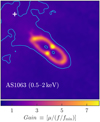 |
Fig. 18. Gain map for the field of AS1063 in the soft band. The contours mark the transition from the region with Gain < 1 to that with Gain > 1, where the magnification due to strong lensing exceeds the sensitivity loss due to the ICM emission and the PSF smearing. The white cross marks the position of the smallest PSF size. |
The next question then is how many Chandra fields with massive clusters, modeled on the CLASH sample, are required in order to investigate the X-ray sky down to the CDFS limits. We can estimate this by requiring a number of sources below a given delensed flux limit comparable to the same flux range at the faint end of the CDFS log N–log S. For example, the CDFS includes about 400 and 160 sources below 5 × 10⁻¹⁷ and 2 × 10⁻¹⁶ erg s−1 cm−2 in the soft and hard band, respectively5. We considered three of the fields with the longest exposure times, M0416, M1206 and AS1063, with 320, 200 and 125 ks, respectively. Then we computed the total number of sources expected from the best fit of the CDFS number counts, using Eq. (3) and Table 8 in Luo et al. (2017). The total number of sources expected in a survey made of Nf fields is
where Ω(S) is the sky coverage in the source plane we computed in each field. Here the contributions from AGN and star-forming galaxies are summed to include all the unresolved sources. We also considered a 20% higher normalization to be consistent with the predictions by the model of Gilli et al. (2007). To match the CDFS in the soft band, we need about 9, 28, and 57 ×103 fields comparable to M0416, M1206, and AS1063, respectively. In the hard band, this number reduces to 3, 7, and 16 ×103 fields. We are aware that this estimate is adequate for the Chandra performances comparable to the actual data, and therefore should not be applied to future Chandra observations, for which the sensitivity in the soft band is unfortunately dramatically lower than in the data we analyzed. Therefore it is not feasible to reach a depth comparable to the CDFS by adding all the fields of massive clusters, which in the Chandra archive and for the considered exposure times are ∼100 − 200. To be fully successful, this program should also rely on optical and spectroscopic data in order to build the magnification maps of the clusters, or on a massive dataset in the optical data. In this respect, the Euclid mission6 will provide a key contribution.
The situation will be similar for future X-ray missions with high angular resolution on a large field of view, such as AXIS (see Marchesi et al. 2020) or Lynx (The Lynx Team 2018). As an exercise, we recomputed Fig. 19, but assuming a flat PSF and a constant Rext = 1 arcsec. This would decrease the background effect in the most interesting regions, close to the critical lines and therefore embedded in the ICM emission. In other words, Slim would be closer to the lowest flux limit achievable in the same field Sfield. The result, shown in Fig. 20, is that the Gain does not increase significantly. However, this simple exercise concerns only the S/N threshold, and does not include the effect of the improved PSF on the source detection, which has an additional positive effect. To summarize, we expect that the efficiency of source detection in the midst of the ICM would improve by a significant factor with the next generation of high-resolution X-ray telescopes, but hardly by an order of magnitude.
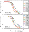 |
Fig. 19. Cumulative solid angle as a function of the Gain in the soft (upper panel) and hard (lower panel) bands. |
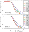 |
Fig. 20. Same as in Fig. 19, but assuming a constant Rext = 1″ everywhere, thus significantly reducing the background effect. |
Clearly, our assessment of the limited effectiveness of strong lensing in the deep exploration of the X-ray sky does not exclude the possibility that a few highly magnified X-ray source are found, particularly when applied to high-redshift star-forming galaxies or multiply-imaged bright AGN. Another possibility is to explore a different mass scale, including groups (with halo masses M200 < 1014 M⊙) and galaxies. The intensity of the ICM rapidly decreases with mass because the bremsstrahlung emission scales with the square of the electron density in the (almost) fully ionized ICM. While we focused our attention first on massive clusters because their magnification is far higher and the extent of the critical lines is larger, the lower mass range offers several advantages: The magnification effect becomes more favorable as a result of the weaker foreground and the number density of groups and low-mass clusters is much higher than in massive clusters. Roughly speaking, the foreground scales with the square of the mass, but the magnification scales only linearly with mass, so that there will be a sweet spot where the search for X-ray lensed sources in Chandra archival data is more efficient. Unfortunately, Chandra archival observations of groups are somewhat limited because most of the telescope time has been used, understandably, to study massive clusters. This approach will be explored in a future paper.
8. Conclusions
Strong gravitational lensing by massive clusters has been shown to be very successful in revealing the properties of very distant, highly magnified galaxies in the optical and IR bands, but it was never explored in the X-ray band because of the intense diffuse emission of the ICM and the low density of X-ray sources. In this work, we performed a systematic search of X-ray lensed sources in the Chandra observations of massive clusters for the first time, employing the exquisite optical (imaging and spectroscopy) dataset of 11 CLASH targets, as well as our high-precision lens models. Our aim was to identify X-ray emission from any unresolved X-ray source magnified by the foreground massive cluster with a readily identified optical counterpart or blindly identified in the X-ray images. Our final goal was to investigate the efficiency of massive galaxy clusters in acting as cosmic telescopes in the X-ray band. Our results are summarized below.
We identified nine X-ray emitting sources corresponding to optical counterparts of lensed sources identified in HST and MUSE data. Three of these (one of which double) are consistent with being powered by star formation, and the other six have X-ray luminosities in the Seyfert range.
We identified 66 X-ray lensed source candidates in the X-ray soft- and hard-band images with untargeted detection using wavdetect and with the requirement of having an S/N > 2 in any of the two bands.
The delensed cumulative number counts are consistent within the uncertainties with the log N–log S predicted by Gilli et al. (2007) after correcting for the sources at z < zcl + 0.1. We still find a marginal excess of 20% at most (with an average of 10% on the full flux range probed) in the delensed log N–log S, where the discrepancy is highest at about 3 × 10⁻¹⁶ and 10−15 erg s−1 cm−2 in the soft and hard bands, respectively. Nevertheless, this discrepancy is smaller than the 1σ combined uncertainty associated with the flux scale and the count statistics.
The combination of magnification and sensitivity loss in the X-ray band due to the ICM diffuse emission results in a limited efficiency of massive clusters as cosmic telescope. The exploration of the deep X-ray sky at the depth level of the CDFS is not feasible given the current size and quality of the Chandra archive.
Overall, we expect that the detection and characterization of strongly lensed X-ray sources in the Chandra fields of massive clusters is not expected to provide significant improvements with respect to currently available deep X-ray surveys. Nevertheless, we plan to extend this work to less massive halos, where the ICM diffuse emission is much weaker, employing the high-resolution observations of groups and galaxies in the Chandra archive, and to simultaneously perform a blind search of AGN-galaxy lensed systems in extragalactic fields. The rare occurrence of strongly magnified sources may be interesting for cosmological tests based on variability of lensed sources with multiple counterparts, and it may constitute an important science case for future high-resolution X-ray telescopes
We did not include the latest refined lensing model for M0416 that has recently been published in Bergamini et al. (2021). Nevertheless, this does not affect our final results.
For a complete documentation of the Chandra PSF see https://cxc.harvard.edu/proposer/POG/html/chap4.html
Acknowledgments
We thank the anonymous referee for his/her constructive comments that helped improve the paper. We thank Bin Luo for providing the data of the sky coverage in the CDFS. A.L., R.G., and P.T. acknowledge financial contribution from the agreement ASI-INAF n.2017-14-H.0. PB acknowledges financial support from ASI through the agreement ASI-INAF n. 2018-29-HH.0. GBC thanks the Max Planck Society for support through the Max Planck Research Group for S.H. Suyu and the academic support from the German Centre for Cosmological Lensing. We acknowledge support from the PRIN MIUR 2017 WSCC32.
References
- Altieri, B., Berta, S., Lutz, D., et al. 2010, A&A, 518, L17 [NASA ADS] [CrossRef] [EDP Sciences] [Google Scholar]
- Atek, H., Richard, J., Kneib, J.-P., et al. 2015, ApJ, 800, 18 [NASA ADS] [CrossRef] [Google Scholar]
- Atek, H., Richard, J., Kneib, J.-P., & Schaerer, D. 2018, MNRAS, 479, 5184 [NASA ADS] [CrossRef] [Google Scholar]
- Bacon, R., Accardo, M., Adjali, L., et al. 2010, Proc. SPIE, 7735, 773508 [Google Scholar]
- Bacon, R., Vernet, J., Borisova, E., et al. 2014, The Messenger, 157, 13 [NASA ADS] [Google Scholar]
- Balestra, I., Mercurio, A., Sartoris, B., et al. 2016, ApJS, 224, 33 [Google Scholar]
- Balucinska-Church, M., & McCammon, D. 1992, ApJ, 400, 699 [Google Scholar]
- Bayliss, M. B., McDonald, M., Sharon, K., et al. 2020, Nat. Astron., 4, 159 [Google Scholar]
- Bergamini, P., Rosati, P., Mercurio, A., et al. 2019, A&A, 631, A130 [NASA ADS] [CrossRef] [EDP Sciences] [Google Scholar]
- Bergamini, P., Rosati, P., Vanzella, E., et al. 2021, A&A, 645, A140 [EDP Sciences] [Google Scholar]
- Biviano, A., Rosati, P., Balestra, I., et al. 2013, A&A, 558, A1 [NASA ADS] [CrossRef] [EDP Sciences] [Google Scholar]
- Bouwens, R. J., Bradley, L., Zitrin, A., et al. 2014, ApJ, 795, 126 [Google Scholar]
- Bouwens, R. J., Illingworth, G. D., Oesch, P. A., et al. 2015, ApJ, 811, 140 [NASA ADS] [CrossRef] [Google Scholar]
- Bouwens, R. J., Oesch, P. A., Illingworth, G. D., Ellis, R. S., & Stefanon, M. 2017, ApJ, 843, 129 [NASA ADS] [CrossRef] [Google Scholar]
- Broadhurst, T. J., Taylor, A. N., & Peacock, J. A. 1995, ApJ, 438, 49 [NASA ADS] [CrossRef] [Google Scholar]
- Caminha, G. B., Grillo, C., Rosati, P., et al. 2016, A&A, 587, A80 [NASA ADS] [CrossRef] [EDP Sciences] [Google Scholar]
- Caminha, G. B., Grillo, C., Rosati, P., et al. 2017a, A&A, 600, A90 [NASA ADS] [CrossRef] [EDP Sciences] [Google Scholar]
- Caminha, G. B., Grillo, C., Rosati, P., et al. 2017b, A&A, 607, A93 [NASA ADS] [CrossRef] [EDP Sciences] [Google Scholar]
- Caminha, G. B., Rosati, P., Grillo, C., et al. 2019, A&A, 632, A36 [CrossRef] [EDP Sciences] [Google Scholar]
- Chen, B., Dai, X., Kochanek, C. S., et al. 2012, ApJ, 755, 24 [Google Scholar]
- Civano, F., Marchesi, S., Comastri, A., et al. 2016, ApJ, 819, 62 [Google Scholar]
- Coe, D., & Moustakas, L. A. 2009, ApJ, 706, 45 [Google Scholar]
- Coe, D., Zitrin, A., Carrasco, M., et al. 2013, ApJ, 762, 32 [Google Scholar]
- Coe, D., Salmon, B., Bradač, M., et al. 2019, ApJ, 884, 85 [Google Scholar]
- Donahue, M., Ettori, S., Rasia, E., et al. 2016, ApJ, 819, 36 [Google Scholar]
- Fan, X. 2006, New Astron. Rev., 50, 665 [Google Scholar]
- Freeman, P. E., Kashyap, V., Rosner, R., & Lamb, D. Q. 2002, ApJS, 138, 185 [Google Scholar]
- Giacconi, R., Rosati, P., Tozzi, P., et al. 2001, ApJ, 551, 624 [Google Scholar]
- Gilli, R., Comastri, A., & Hasinger, G. 2007, A&A, 463, 79 [NASA ADS] [CrossRef] [EDP Sciences] [Google Scholar]
- Grillo, C., Suyu, S. H., Rosati, P., et al. 2015, ApJ, 800, 38 [NASA ADS] [CrossRef] [Google Scholar]
- Grillo, C., Rosati, P., Suyu, S. H., et al. 2020, ApJ, 898, 87 [Google Scholar]
- Hasinger, G., Miyaji, T., & Schmidt, M. 2005, A&A, 441, 417 [NASA ADS] [CrossRef] [EDP Sciences] [Google Scholar]
- Jauzac, M., Mahler, G., Edge, A. C., et al. 2019, MNRAS, 483, 3082 [NASA ADS] [CrossRef] [Google Scholar]
- Johnson, T. L., & Sharon, K. 2016, ApJ, 832, 82 [NASA ADS] [CrossRef] [Google Scholar]
- Karman, W., Caputi, K. I., Caminha, G. B., et al. 2017, A&A, 599, A28 [NASA ADS] [CrossRef] [EDP Sciences] [Google Scholar]
- Kelly, P. L., Rodney, S. A., Treu, T., et al. 2015, Science, 347, 1123 [NASA ADS] [CrossRef] [Google Scholar]
- Kneib, J.-P., & Natarajan, P. 2011, A&ARv, 19, 47 [NASA ADS] [CrossRef] [Google Scholar]
- Komatsu, E., Smith, K. M., Dunkley, J., et al. 2011, ApJS, 192, 18 [NASA ADS] [CrossRef] [Google Scholar]
- Lagattuta, D. J., Richard, J., Clément, B., et al. 2017, MNRAS, 469, 3946 [Google Scholar]
- Liu, A., Tozzi, P., Ettori, S., et al. 2020a, A&A, 637, A58 [CrossRef] [EDP Sciences] [Google Scholar]
- Liu, T., Merloni, A., Simm, T., et al. 2020b, ApJS, 250, 32 [Google Scholar]
- Lotz, J. M., Koekemoer, A., Coe, D., et al. 2017, ApJ, 837, 97 [Google Scholar]
- Luo, B., Brandt, W. N., Xue, Y. Q., et al. 2017, ApJS, 228, 2 [Google Scholar]
- Mahler, G., Richard, J., Clément, B., et al. 2018, MNRAS, 473, 663 [Google Scholar]
- Marchesi, S., Gilli, R., Lanzuisi, G., et al. 2020, A&A, 642, A184 [EDP Sciences] [Google Scholar]
- Masini, A., Hickox, R. C., Carroll, C. M., et al. 2020, ApJS, 251, 2 [Google Scholar]
- Meneghetti, M., Melchior, P., Grazian, A., et al. 2008, A&A, 482, 403 [NASA ADS] [CrossRef] [EDP Sciences] [Google Scholar]
- Meneghetti, M., Rasia, E., Merten, J., et al. 2010, A&A, 514, A93 [NASA ADS] [CrossRef] [EDP Sciences] [Google Scholar]
- Meneghetti, M., Rasia, E., Vega, J., et al. 2014, ApJ, 797, 34 [Google Scholar]
- Meneghetti, M., Natarajan, P., Coe, D., et al. 2017, MNRAS, 472, 3177 [Google Scholar]
- Meneghetti, M., Davoli, G., Bergamini, P., et al. 2020, Science, 369, 1347 [Google Scholar]
- Merten, J., Meneghetti, M., Postman, M., et al. 2015, ApJ, 806, 4 [Google Scholar]
- Metcalfe, L., Kneib, J. P., McBreen, B., et al. 2003, A&A, 407, 791 [NASA ADS] [CrossRef] [EDP Sciences] [MathSciNet] [Google Scholar]
- Monna, A., Seitz, S., Balestra, I., et al. 2017, MNRAS, 466, 4094 [NASA ADS] [Google Scholar]
- Nanni, R., Gilli, R., Vignali, C., et al. 2020, A&A, 637, A52 [CrossRef] [EDP Sciences] [Google Scholar]
- Ota, N., Inada, N., Oguri, M., et al. 2006, ApJ, 647, 215 [Google Scholar]
- Ota, N., Oguri, M., Dai, X., et al. 2012, ApJ, 758, 26 [Google Scholar]
- Paolillo, M., Papadakis, I., Brandt, W. N., et al. 2017, MNRAS, 471, 4398 [NASA ADS] [CrossRef] [Google Scholar]
- Patrício, V., Richard, J., Carton, D., et al. 2018, MNRAS, 477, 18 [NASA ADS] [CrossRef] [Google Scholar]
- Plazas, A. A., Meneghetti, M., Maturi, M., & Rhodes, J. 2019, MNRAS, 482, 2823 [Google Scholar]
- Postman, M., Coe, D., Benítez, N., et al. 2012, ApJS, 199, 25 [NASA ADS] [CrossRef] [Google Scholar]
- Refregier, A., & Loeb, A. 1996, in Roentgenstrahlung from the Universe, eds. H. U. Zimmermann, J. Trümper, & H. Yorke, 611 [Google Scholar]
- Refregier, A., & Loeb, A. 1997, ApJ, 478, 476 [Google Scholar]
- Richards, G. T., Strauss, M. A., Fan, X., et al. 2006, AJ, 131, 2766 [Google Scholar]
- Robertson, B. E., Ellis, R. S., Furlanetto, S. R., & Dunlop, J. S. 2015, ApJ, 802, L19 [Google Scholar]
- Rosati, P., Tozzi, P., Giacconi, R., et al. 2002, ApJ, 566, 667 [Google Scholar]
- Salmon, B., Coe, D., Bradley, L., et al. 2018, ApJ, 864, L22 [NASA ADS] [CrossRef] [Google Scholar]
- Salmon, B., Coe, D., Bradley, L., et al. 2020, ApJ, 889, 189 [Google Scholar]
- The Lynx Team 2018, ArXiv e-prints [arXiv:1809.09642] [Google Scholar]
- Umetsu, K., Sereno, M., Tam, S.-I., et al. 2018, ApJ, 860, 104 [NASA ADS] [CrossRef] [Google Scholar]
- Vanzella, E., Calura, F., Meneghetti, M., et al. 2017a, MNRAS, 467, 4304 [Google Scholar]
- Vanzella, E., Balestra, I., Gronke, M., et al. 2017b, MNRAS, 465, 3803 [NASA ADS] [CrossRef] [Google Scholar]
- Vanzella, E., Calura, F., Meneghetti, M., et al. 2019, MNRAS, 483, 3618 [NASA ADS] [CrossRef] [Google Scholar]
- Vanzella, E., Caminha, G. B., Rosati, P., et al. 2021, A&A, 646, A57 [EDP Sciences] [Google Scholar]
- Willingale, R., Starling, R. L. C., Beardmore, A. P., Tanvir, N. R., & O’Brien, P. T. 2013, MNRAS, 431, 394 [NASA ADS] [CrossRef] [Google Scholar]
- Yue, B., Ferrara, A., Vanzella, E., & Salvaterra, R. 2014, MNRAS, 443, L20 [Google Scholar]
- Zitrin, A., Zheng, W., Broadhurst, T., et al. 2014, ApJ, 793, L12 [Google Scholar]
Appendix A: X-ray lensed source candidates with multiple counterparts
We have identified five multiply lensed sources (labeled “(m)” in Table 3) as X-ray emitter candidates in the optically lensed sources. Because in each case only one counterpart has an X-ray signal, we can therefore check whether the detection is consistent with the aperture photometry at the position of the other optical counterparts (assuming that variability does not play a role for simplicity). Source AS1063−46 is detected only in the soft band with 17.5 ± 8.6 net counts and a magnification of ∼30, and it has two other counterparts with a magnification of 3.4 and 17.8. The first counterpart would be clearly too faint to be visible, but the second is expected to have ∼10 net counts, which does not significantly contradict with the aperture photometry at its position, which is 2.1 ± 6.0 net counts. AS1063−95, detected in the soft band with photometry 9.7 ± 5.1, has two counterparts with similar magnification, whose photometry provides 4.3 ± 6.9 and 22.5 ± 16.4 net counts in the soft band, consistent with the photometry of the candidate X-ray emitters. Source M0416−221 is detected with 7.3 ± 4.1 net counts in the soft band and has two counterparts with photometry −1.0 ± 9.8 and 3.0 ± 4.4, where 7 and 10 net counts were expected, respectively. The nondetection of the two other counterparts does not create a significant discrepancy with our X-ray detection in this case either. For sources AS1063−46, AS1063−95, and M0416−221, our X-ray detection is therefore consistent with no detection at the position of the other counterparts.
Source M0416−208 is detected in the soft band with 15.6 ± 5.5 net counts. It has two counterparts that are expected to measure 30 and 14 counts in the same band. However, the photometry on the two counterparts gives −2.2 ± 7.4 and −0.6 ± 8.4. The situation is the same for M0416−241, for which we have a detection with 15.3 ± 7.8 net counts in the hard band. There is another counterpart of this source, with higher magnification, for which about 30 net counts are expected, while its photometry is 2.0 ± 4.7, which is therefore inconsistent at more than 3σ. We conclude that M0416−208 and M0416−241 should be removed from our candidate list.
All Tables
X-ray emitting sources identified by visual inspection at the position of optically lensed sources.
Fractional distribution in bins of redshift for the sources of the CDFS (normalized total number of sources in the range 0.5 < z < 4).
All Figures
|
Fig. 1. Solid angle as a function of magnification and redshift for M0416. Left panel: cumulative solid angle corresponding to a magnification higher than a given value A(> μ) in the lens plane plotted as a function of magnification for a set of redshifts from 1 to 6 for the cluster M0416 at z = 0.397. The maximum solid angle corresponds to the 25 arcmin2 surveyed area in each cluster. Right panel: cumulative solid angle A(> μ) for μ = 10, 20, 50, and 100 in the lens plane as a function of the redshift of the lensed source for the cluster M0416. |
| In the text | |
|
Fig. 2. Solid angle as a function of magnification and redshift for the 11 clusters. Left panel: solid angle A(> μ) in the lens plane for each of the 11 clusters as a function of μ(zs = 6). Right panel: cumulative solid angle A(> μ) in the lens plane for our entire sample for a source redshift from 1 to 6. The vertical dashed line shows the lower magnification limit μmax = 1.5 that defines the field of view we investigated. |
| In the text | |
|
Fig. 3. Solid angle A(μ > 10) in the lens plane computed for z = 6, plotted against the virial mass computed within r200 from the weak-lensing measurements of Umetsu et al. (2018). Masses of M1311 and M2129 are based on X-ray scaling relations according to Liu et al. (2020a). The dashed line shows the best-fit linear relation A = 0.08 × (M200/1014 M⊙)−0.17 as a reference to appreciate the slope of the relation in our sample. |
| In the text | |
|
Fig. 4. Examples of identified X-ray counterparts of optically lensed sources. Left panels: residual X-ray images (soft band), and right panels: HST images. Contours are those used for aperture photometry in the X-ray bands. Top panels: source 23 in the FOV of M1115, with μ ∼ 74. Middle panels: source 46 in the FOV of AS1063, with μ ∼ 30. Bottom panels: sources 12, 13 (elongated region), and 73 (circular region) in the FOV of R2129, with μ ∼ 1.5, 1.5, and 1.9, respectively. |
| In the text | |
|
Fig. 5. Redshift and magnification of the sources in Table 3 identified by visual inspection after removing the two sources marked with the asterisk. The 1σ error on magnification is about 10% up to μ = 10, and it can reach a factor of 2 or higher for μ > 20. |
| In the text | |
|
Fig. 6. Histogram of aperture-photometry values in the soft and hard bands (cyan and orange histogram, respectively) for the 837 optically lensed sources in the 11 cluster fields after removing the visually identified sources listed in Table 3. The thick solid lines show the normalized best-fit Gaussian functions. |
| In the text | |
|
Fig. 7. Stacked X-ray image of all the optically identified lensed sources after removing the 11 X-ray detected sources and clipping the extreme photometry values as described in the text. Images are 10″ across, and the color scale indicates net counts. Upper and lower panels: soft and hard bands, respectively. The white circle marks the 3 arcsec aperture we used for photometry in the stacked images. |
| In the text | |
|
Fig. 8. Comparison of the aperture photometry values obtained with modeled or directly sampled background and foreground for the soft band (upper panel) and hard band (lower panel). The solid line shows the x = y relation. |
| In the text | |
|
Fig. 9. Distribution of observed and delensed fluxes in the soft (upper panel) and hard (lower panel) bands for the sources detected with our algorithm (Table 6) plus sources with optical counterpart (as in Table 3). Only sources with S/N ≥ 2 in each band are shown. |
| In the text | |
|
Fig. 10. Scatter plot of the soft (top panel) and hard (bottom panel) observed flux vs. the weighted magnification. Top panel: the region below the solid and dashed black lines corresponds to delensed fluxes below 10−16 and 10−17 erg s−1 cm−2, respectively. Bottom panel: the region below the black line corresponds to delensed fluxes below 10−15 erg s−1 cm−2. Sources marked with circles are X-ray selected, and triangles correspond to sources identified as X-ray counterparts of optically lensed sources (listed in Table 3). Only sources with S/N ≥ 2 in each band are shown. |
| In the text | |
|
Fig. 11. Completeness maps in the 0.5−2 keV band for all the sources with S/N > 2 detected with wavdetect in the 11 cluster fields. The color code indicates the completeness or recovery rate at a given input net counts N, as shown in the color bar, in the 0.5−2 keV band. The maps are 5′ across and are smoothed with a Gaussian FWHM of 10″. The black crosses mark the position of minimum PSF in each field, resulting from the overlapping of several exposures with different aim points. The low recovery rates in cluster centers and in the corners of the field of view are due to the strong ICM emission and the increase in PSF size, respectively. |
| In the text | |
|
Fig. 12. Cumulative number of spurious sources N expected per field with measured net counts below C for each cluster in the soft (upper panel) and hard (lower panel) bands. |
| In the text | |
|
Fig. 13. Ratio of spurious sources over detected sources in the entire survey in bins of observed net counts in the soft (top panel) and hard (bottom panel) bands. |
| In the text | |
|
Fig. 14. Sky coverage as a function of flux for the 11 CLASH cluster fields. The thick solid curve shows the sky coverage in the source plane as a function of the de-lensed flux in the soft (left panel) and hard (right panel) bands. The thick dotted curve instead shows the same sky coverage in the source plane, but as a function of the observed flux. The sky coverage in the source plane was used to compute the delensed log N–log S. The sky coverage in the lens plane is also shown as a function of the delensed flux (continuous curve) and of the observed flux (thin dotted curve). The horizontal dashed line indicates the total solid angle, by the criterion μmax > 1.5. The black curve shows the sky coverage of the 7 Ms CDFS survey in the corresponding energy ranges (Luo et al. 2017). The hard-band flux limits in Luo et al. (2017) given in 2−7 keV are converted into 2−10 keV by assuming Γ = 1.8. |
| In the text | |
|
Fig. 15. Effects of the cuts in redshift for zs < zcl + 0.1 on the expected log N–log S of lensed X-ray sources in the soft (upper panel) and hard (lower panel) bands. The upper red lines show the total number counts from the model by Gilli et al. (2007), and the lower blue lines show the number counts expected for the lensed sources (zs < zcl + 0.1) on the basis of Gilli et al. (2007). The shaded areas are the CDFS number counts from Luo et al. (2017). The hard-band flux limits in Luo et al. (2017) given in 2−7 keV are converted into 2−10 keV by assuming Γ = 1.8. The predictions from Gilli et al. (2007) are multiplied by a factor of 0.8 to be consistent with the CDFS results. |
| In the text | |
|
Fig. 16. Number counts of sources detected in the CLASH fields as a function of flux. Left panels: cumulative number counts of the lensed sources in the soft band (upper left) and hard band (lower left). The number counts are compared with the prediction by the model of Gilli et al. (2007) after removing the foreground sources. Right panels: effects of the flux magnification and source dilution shown separately in the soft band (upper right) and hard band (lower right). |
| In the text | |
|
Fig. 17. Flux limit corresponding to the selection criterion S/N > 2 in the soft band for the AS1063 field. The observed flux limit is shown in the left panel, and the delensed flux limit is shown in the right panel. The images are 5′ across and are smoothed with an FWHM of 3″. |
| In the text | |
|
Fig. 18. Gain map for the field of AS1063 in the soft band. The contours mark the transition from the region with Gain < 1 to that with Gain > 1, where the magnification due to strong lensing exceeds the sensitivity loss due to the ICM emission and the PSF smearing. The white cross marks the position of the smallest PSF size. |
| In the text | |
|
Fig. 19. Cumulative solid angle as a function of the Gain in the soft (upper panel) and hard (lower panel) bands. |
| In the text | |
|
Fig. 20. Same as in Fig. 19, but assuming a constant Rext = 1″ everywhere, thus significantly reducing the background effect. |
| In the text | |
Current usage metrics show cumulative count of Article Views (full-text article views including HTML views, PDF and ePub downloads, according to the available data) and Abstracts Views on Vision4Press platform.
Data correspond to usage on the plateform after 2015. The current usage metrics is available 48-96 hours after online publication and is updated daily on week days.
Initial download of the metrics may take a while.