| Issue |
A&A
Volume 648, April 2021
|
|
|---|---|---|
| Article Number | A120 | |
| Number of page(s) | 26 | |
| Section | Interstellar and circumstellar matter | |
| DOI | https://doi.org/10.1051/0004-6361/202040112 | |
| Published online | 26 April 2021 | |
Gas phase Elemental abundances in Molecular cloudS (GEMS)
IV. Observational results and statistical trends
1
Observatorio Astronómico Nacional (OAN),
Alfonso XII, 3,
28014
Madrid, Spain
e-mail: This email address is being protected from spambots. You need JavaScript enabled to view it.
2
Centre for Astrochemical Studies, Max-Planck-Institute for Extraterrestrial Physics,
Giessenbachstrasse 1,
85748
Garching, Germany
3
Observatoire de Paris, PSL Research University, CNRS, École Normale Supérieure, Sorbonne Universités, UPMC Univ. Paris 06,
75005
Paris, France
4
Institut de Radioastronomie Millimétrique,
300 rue de la Piscine, Domaine Universitaire,
38406
Saint Martin d’Hères, France
5
LERMA, Observatoire de PARIS, PSL Research University, CNRS, Sorbonne Université,
92190
Meudon, France
6
Laboratoire d’astrophysique de Bordeaux, Univ. Bordeaux, CNRS, B18N, allée Geoffroy Saint-Hilaire,
33615
Pessac, France
7
Harvard-Smithsonian Center for Astrophysics,
60 Garden St.,
Cambridge,
MA 02138, USA
8
Faculty of Aerospace Engineering, Delft University of Technology,
Delft, The Netherlands
9
University of Leiden,
PO Box 9513,
NL,
2300 RA
Leiden, The Netherlands
10
École Normale Supérieure de Lyon, CRAL, UMR CNRS 5574, Université Lyon I,
46 allée d’Italie,
69364
Lyon Cedex 07, France
11
Instituto de Física Fundamental (CSIC),
Calle Serrano 123,
28006
Madrid, Spain
12
Institut des Sciences Moléculaires (ISM), CNRS, Univ. Bordeaux,
351 cours de la Libération,
33400
Talence, France
13
Chalmers University of Technology, Department of Space,
Earth and Environment,
412 93
Gothenburg, Sweden
14
Centro de Astrobiología (CSIC-INTA),
Ctra. de Ajalvir, km 4,
Torrejón de Ardoz,
28850
Madrid, Spain
15
University of Vienna, Department of Astrophysics,
Tuerkenschanzstrasse 17,
1180
Vienna, Austria
16
Jeremiah Horrocks Institute, University of Central Lancashire,
Preston
PR1 2HE, UK
17
Observatorio de Yebes (IGN). Cerro de la Palera s/n,
19141
Yebes, Spain
18
Department of Physics, University of Helsinki,
PO Box 64,
00014
Helsinki, Finland
19
Institute of Physics I, University of Cologne,
Cologne, Germany
20
National Radio Astronomy Observatory,
520 Edgemont Rd.,
Charlottesville
VA 22901, USA
Received:
10
December
2020
Accepted:
10
February
2021
Abstract
Gas phase Elemental abundances in Molecular CloudS (GEMS) is an IRAM 30 m Large Program designed to provide estimates of the S, C, N, and O depletions and gas ionization degree, X(e−), in a selected set of star-forming filaments of Taurus, Perseus, and Orion. Our immediate goal is to build up a complete and large database of molecular abundances that can serve as an observational basis for estimating X(e−) and the C, O, N, and S depletions through chemical modeling. We observed and derived the abundances of 14 species (13CO, C18O, HCO+, H13CO+, HC18O+, HCN, H13CN, HNC, HCS+, CS, SO, 34SO, H2S, and OCS) in 244 positions, covering the AV ~3 to ~100 mag, n(H2) ~ a few 103 to 106 cm−3, and Tk ~10 to ~30 K ranges in these clouds, and avoiding protostars, HII regions, and bipolar outflows. A statistical analysis is carried out in order to identify general trends between different species and with physical parameters. Relations between molecules reveal strong linear correlations which define three different families of species: (1) 13CO and C18O isotopologs; (2) H13CO+, HC18O+, H13 CN, and HNC; and (3) the S-bearing molecules. The abundances of the CO isotopologs increase with the gas kinetic temperature until TK ~ 15 K. For higher temperatures, the abundance remains constant with a scatter of a factor of ~3. The abundances of H13 CO+, HC18 O+, H13 CN, and HNC are well correlated with each other, and all of them decrease with molecular hydrogen density, following the law ∝ n(H2)−0.8 ± 0.2. The abundances of S-bearing species also decrease with molecular hydrogen density at a rate of (S-bearing/H)gas ∝ n(H2)−0.6 ± 0.1. The abundances of molecules belonging to groups 2 and 3 do not present any clear trend with gas temperature. At scales of molecular clouds, the C18O abundance is the quantity that better correlates with the cloud mass. We discuss the utility of the 13CO/C18O, HCO+/H13CO+, and H13 CO+/H13CN abundance ratios as chemical diagnostics of star formation in external galaxies.
Key words: astrochemistry / ISM: abundances / ISM: molecules / ISM: clouds / stars: formation / galaxies: ISM
© ESO 2021
1 Introduction
Gas chemistry plays a key role in the star formation process by regulating fundamental parameters such as the gas cooling rate and ionization fraction. Molecular clouds can contract and fragment because molecules cool the gas, thus diminishing the thermal support relative to self-gravity. The ionization fraction controls the coupling of magnetic fields with the gas, driving the dissipation of turbulence and angular momentum transfer, and therefore plays a crucial role in cloud collapse (isolated vs. clustered star formation) and the dynamics of accretion disks (see Zhao et al. 2016; Padovani et al. 2013). In the absence of other ionization agents (X-rays, UV photons, J-type shocks), the steady state ionization fraction is proportional to  , where n is the molecular hydrogen density and
  is the cosmic-ray ionization rate for H2 molecules, which becomes the key parameter in the molecular cloud evolution (Oppenheimer & Dalgarno 1974; McKee 1989; Caselli et al. 2002). The gas ionization fraction, X(e−) = n(e−)/nH, and molecular abundances depend on the elemental depletion factors (Caselli et al. 1998). In particular, carbon (C) is the main donor of electrons in the cloud surface region (AV < 2 mag), and because of its lower ionization potential and as long as it is not heavily depleted, sulfur (S) is the main donor in the ~3.7−7 magnitudes range that encompasses a large fraction of the molecular cloud mass (Goicoechea et al. 2006). As CO and [CII] are the main coolants, depletions of C and O determine the gas cooling rate in molecular clouds.
Elemental depletions also constitute a valuable piece of information for our understanding of the grain composition and evolution. For any given element, the missing atoms in the gas phase are presumed to be locked up in solids, that is, dust grains and/or icy mantles. Knowledge of elemental depletions can therefore be valuable in studying the changes in the dust grain composition across the cloud. Surface chemistry and the interchange of molecules between the solid and gas phases have a leading role in the chemical evolution of gas from the diffuse cloud to the prestellar core phase.
GEMS Gas phase Elemental abundances in Molecular CloudS (GEMS) is an IRAM 30 m Large Program, the aim of which is to estimate the S, C, N, and O depletions and X(e−) as a function of visual extinction in a selected set of prototypical star-forming filaments. Regions with different illumination are included in the sample in order to investigate the influence of UV radiation (photodissociation, ionization, photodesorption) and turbulence on these parameters, and eventually in the star formation history of the cloud. The depletion factor is defined as the ratio between the total (dust+gas) abundance of a given element and its abundance as observed in the gas phase. The determination of the depletion factor of a given element can only been done directly through high-sensitivity observations of the main molecular reservoirs of each element and detailed chemical modeling of the secondary reservoirs (Fuente et al. 2019, see a simple scheme in Fig. 1).
The first step to derive the elemental gas abundance of C, O, N, and S is to determine the abundances of the main reservoirs of the elements in the gas phase. Essentially, most of the carbon is locked in CO in dense cores and the C depletion is derived from the study of CO and its isotopologs. A significant fraction of C may be atomic (C, C+) in the molecular gas surrounding the cores. The gas ionization fraction, X(e−), can be derived from the [HCO+]/[CO] ratio, whichcan help to constrain the C depletion values through comparison with chemical models. The main reservoirs of nitrogen are supposed to be atomic nitrogen (N) and molecular nitrogen (N2) which are not observable. The nitrogen abundance can be derived by applying a chemical model to fit the observed abundances of nitriles (HCN, HNC, CN) (Agúndez & Wakelam 2013; Le Gal et al. 2014). The HCN abundance is also dependent on the amount of atomic C in gas phase, mainly on the C/O ratio (Loison et al. 2014; Fuente et al. 2016). The most abundant oxygenated molecules, O2, H2O, and OH, are difficult to observe in the millimeter domain and the oxygen depletion factor has to be derived indirectly from the C/O ratio. The CS/SO abundance ratio has been used as a proxy for the C/O ratio in different environments (Fuente et al. 2016; Semenov et al. 2018). The abundances of other species such as HCN and C2 H are also very sensitive to the C/O gas-phase ratio (Loison et al. 2014; Miotello et al. 2019).
Determining sulfur depletion is challenging. Sulfur is one of the most abundant elements in the Universe (S∕H ~ 1.5 × 10⁻⁵) (Asplund et al. 2009) and plays a crucial role in biological systems on Earth, and so it is important to follow its chemical history in space (i.e., toward precursors of Solar System analogs). Surprisingly, S-bearing molecules are not as abundant as expected in the interstellar medium. Sulfur is thought to be depleted in molecular clouds by a factor up to 1000 compared to its estimated cosmic abundance (Ruffle et al. 1999; Wakelam et al. 2004). Because of the high hydrogen abundances and the mobility of hydrogen in the ice matrix, sulfur atoms in interstellar ice mantles are expected to preferentially form H2S. There are only upper limits to the solid H2S abundance (e.g., Jiménez-Escobar & Muñoz Caro 2011), and OCS is the only S-bearing molecule unambiguously detected in ice mantles because of its large band strength in the infrared (Geballe et al. 1985; Palumbo et al. 1995) along with, tentatively, SO2 (Boogert et al. 1997). One possibility is that most of the sulfur is locked in atomic sulfur in the gas phase. Also, sulfur could be in refractory allotropes, mainly S8, as found theoretically by Shingledecker et al. (2020), and previously observed in the laboratory by Jiménez-Escobar et al. (2012, 2014). The detection of sulfur allotropes in comets (Calmonte et al. 2016) and of S2 H in gas phase (Fuente et al. 2017) testify to the importance of these compounds. Unfortunately, sulfur allotropes cannot be directly observed in the interstellar medium. Direct observation of the S atom is also difficult and, until now, S has only been detected in some bipolar outflows using the infrared space telescope Spitzer (Anderson et al. 2013). Our project includes a wide set of S-bearing species (CS, SO, H2S, HCS+, SO2, OCS, and H2CS) that are going to be used to constrain the sulfur depletion in our sample. To our knowledge, this will constitute the most complete database of S-bearing molecules in dark clouds so far.
A detailed presentation of the project with a list of species and isotopologs observed was included in Fuente et al. (2019). This paper presents the abundances of 13CO, C18O, CS, C34S, 13CS, H2S, SO, 34SO, HCO+, H13 CO+, HC18O+, HCN, H13CN, HNC, HCS+, and OCS towards the whole sample. Our goal is to investigate the statistical trends of these molecular abundances and their dependency on the local physical conditions as a first step toward understanding the chemical evolution of dark clouds.Detailed chemical modeling of each region, which constitutes an imperative step toward deriving elemental abundances (see Fig. 1), will be carried out in a future paper. The observations of N2 H+ will also be presented elsewhere since, as discussed by Fuente et al. (2019), they require a more sophisticated modeling. We do not include H2CS, because it has only been detected in a small fraction of the observed positions, preventing a statistical analysis.
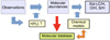 |
Fig. 1 Block diagram of the GEMS project. |
2 Sample selection
Our project focuses on the nearby star forming regions Taurus, Perseus, and Orion. These molecular cloud complexes were observed with Herschel and SCUBA as part of the Gould Belt Survey (André et al. 2010), and accurate visual extinction (AV) and dust temperature(Td) maps are available (Malinen et al. 2012; Hatchell et al. 2005; Lombardi et al. 2014; Zari et al. 2016). The angular resolution of the AV -Td maps (~36″) is similar to that provided by the 30 m telescope at 3mm allowing direct comparison of continuum and spectroscopic data. Throughout this paper we adopt the relation between visual extinction and molecular hydrogen column density AV ≈ N(H2) × 10−21 mag (Bohlin et al. 1978).
These regions are characterized as having different star formation activity and therefore different illumination. This allows us to investigate the influence of UV radiation on the gas composition. Our strategy is to observe several starless cores within each filament. By comparing the cores in the same filament, we will be able to investigate the effect of time evolution on the chemistry of dark cores (see, e.g., Frau et al. 2012). By comparing cores in different regions, we explore the effect of the environment on the chemistry therein. The list of selected cores is shown in Table 1.
Within the pilot project, we observed three cuts in TMC1 and one in Barnard 1b whose data have been partially published in Fuente et al. (2019) and Navarro-Almaida et al. (2020). The data from these cuts are included in this paper for completeness.
In total, our project includes observations towards 305 positions distributed in 27 cuts roughly perpendicular to the selected filaments. The cuts are designed to intersect the filament along one of the selected starless cores, avoiding the position of known protostars, HII regions, and bipolar outflows. They cover visual extinctions from AV ~ 3 mag up to AV ~ 200 mag in the line of sight towards the giant molecular cloud Orion A. The separation between one position and another in a given cut is selected to sample the visual extinction range in regular intervals of AV. However, this is not always possible, specially for AV > 10 mag, where the surface density gradient is steeper. At low visual extinctions, not all the lines are detected. In this paper, we only consider 244 positions for which we are able to determine the gas density from the CS and its isotopolog observations (see Sect. 4). In the following, we describe the observed positions in more detail:
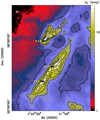 |
Fig. 2 TMC1 visual extinction map (Kirk et al., in prep.). Positions observed with the 30 m telescope are indicated with circles. Black circles mark positions observed only with the 30 m telescope, while yellow circles indicate positions also observed with the Yebes 40 m telescope. |
Taurus: TMC 1, B213/L1495
The Taurus molecular cloud (TMC), at a distance of 145 pc (Yan et al. 2019), is considered an archetypal low-mass star-forming region. It has been the target of several cloud evolution and star formation studies (Ungerechts & Thaddeus 1987; Mizuno et al. 1995; Goldsmith et al. 2008), being extensively mapped in CO (Cernicharo & Guelin 1987; Onishi et al. 1996; Narayanan et al. 2008) and visual extinction (Cambrésy 1999; Padoan et al. 2002; Schmalzl et al. 2010).
In the pilot project we centered on the filament TMC 1, which has been the target of numerous chemical studies. In particular, the positions TMC 1-CP and TMC 1-NH3 (the cyanopolyynes and ammonia emission peaks) are generally adopted as templates to compare with chemical codes (e.g., Fehér et al. 2016; Gratier et al. 2016; Agúndez & Wakelam 2013). Less studied from a chemical point of view, TMC 1-C has been identified as an accreting starless core (Schnee et al. 2007, 2010). Within GEMS, we observed three cuts across the TMC 1-CP, TMC 1-NH3, and TMC 1-C (see Fig. 2). Fuente et al. (2019) carried out a complete analysis of these data to derive the gas ionization degree and elemental abundances.
In this work, we use the H2 column density and dust temperature maps of TMC 1 created following the process described in Kirk et al. (2013) and Fuente et al. (2019) on the basis of Herschel (Poglitsch et al. 2010; Griffin et al. 2010) data taken as part of the Herschel Gould Belt Survey (André et al. 2010) and Planck data (cf. Bernard et al. 2010). The data were convolved to the resolution of the longest wavelength, 500 μm (36 arcsec). The typical uncertainty on the fitted dust temperature was 0.3–0.4 K. The uncertainty on the column density was typically 10% and reflects the assumed calibration error of the Herschel maps.
B213/L1495 is a prominent filament in Taurus that has received a lot of recent observational attention (Palmeirim et al. 2013; Hacar et al. 2013; Marsh et al. 2014; Tafalla & Hacar 2015; Bracco et al. 2017; Shimajiri et al. 2019). A population of dense cores previously studied in emission lines of high-dipole-moment species, such as NH3, H13 CO+, and N2 H+, are embedded in this filament (Benson & Myers 1989; Onishi et al. 2002; Tatematsu et al. 2004; Hacar et al. 2013; Punanova et al. 2018). Some of these dense cores are starless, while others are associated with young stellar objects (YSOs) of different ages. This population of YSOs has been the subject of a number of dedicated studies, most recently by Luhman et al. (2009) and Rebull et al. (2010), and by the dedicated outflow search by Davis et al. (2010). Interestingly, the density of stars decreases from north to south suggesting a different dynamical and chemical age along the filament. The morphology of the map with striations perpendicular to the filament suggests that the filament is accreting material from its surroundings (Goldsmith et al. 2008; Palmeirim et al. 2013). Shimajiri et al. (2019) proposed that this active star-forming filament was initially formed by large-scale compression of HI gas and is now growing in mass due to the gravitational accretion of molecular gas from ambient cloud. We observed nine cuts along clumps #1, # 2, #5, #6, #7, #9, #12, #16, and #17 (core numbers from the catalog of Hacar et al. 2013).
In this work, we use the H2 column density and dust temperature maps of B213 (see Fig. 3) obtained by Palmeirim et al. (2013) on the basis of the Herschel Gould Belt Survey (André et al. 2010) and Planck data (cf. Bernard et al. 2010) at an angular resolution of 18.2″.
Perseus: Barnard 1, NGC 1333, IC 348, L1448, B5
The Perseus molecular cloud is a well-known star-forming cloud in the Galaxy, at a distance of 310 pc (Ortiz-León et al. 2018). The cloud was extensively studied using molecular line emission (Warin et al. 1996; Ridge et al. 2006; Curtis & Richer 2011; Pineda et al. 2008, 2010, 2015; Friesen et al. 2017; Hacar et al. 2017b), star count extinction (Bachiller & Cernicharo 1984), and dust continuum emission (Hatchell et al. 2005; Kirk et al. 2006; Enoch et al. 2006; Zari et al. 2016). The molecular cloud complex is associated with two clusters containing pre-main-sequence stars: IC 348, with an estimated age of 2 Myr (Luhman et al. 2003); NGC 1333, which is younger than 1 Myr in age (Lada et al. 1996; Wilking et al. 2004); and the Per 0B2 association, which contains a B0.5 star (Steenbrugge et al. 2003).
Perseus is the prototype low- and intermediate-mass star- forming region. The molecular cloud itself contains numerous protostars and dense cores. Hatchell et al. (2005) presented a survey of dense cores in the Perseus molecular cloud using continuum maps at 850 and 450 μm with SCUBA at the JCMT. They detected a total of 91 protostars and starless cores (Hatchell et al. 2007b). Later, Hatchell et al. (2007a) surveyed the outflow activity in the region to characterize the populations of protostars. In contrast with Taurus, a significant fraction of these protostars are associated in protoclusters, unveiling a different star formation regime. Within GEMS, we observed 11 cuts along starless cores distributed in Barnard 1, IC 348, L1448, NGC 1333, and B5 (see Fig. 4). The group of cores in IC 348 and NGC 1333 are close to the clusters and therefore immersed in a harsh environment, while Barnard 1 and L1448 are located in a quiescent region.
We use the dust opacity and dust-temperature maps reported by Zari et al. (2016) in our analysis (see Fig. 4). In order to derive the molecular hydrogen column density from the dust opacity at 850 μm (τ850), we used expression (7) of Zari et al. (2016) and AV = AK/0.112. This expression gives accurate values for low extinctions (AV < 10 mag) but may underestimate their value towards the extinction peaks. In the range of values considered in Perseus, AV ~ 3 −30 mag, the uncertainty in the values of AV is a factor of two.
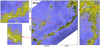 |
Fig. 3 B213 molecular hydrogen column density maps as derived by Palmeirim et al. (2013), reconstructed at an angular resolution of 18.2″. General view of the region is represented at the center, and main regions of interest are enlarged. Contours are (3, 6, 9,12, 15, 20, and 25) × 1021 cm−2. Positions observed by GEMS with the 30 m telescope are indicated with triangles. Green triangles represent the position of the starless cores. Labels in red indicate the cut IDs. See Table 1 for further details. |
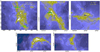 |
Fig. 4 Perseus filaments (from left to right and top to bottom: NGC 1333, Barnard 1, IC 348, L1448, and B5) dust opacity maps at 850 μm by Zari et al. (2016), convolved at an angular resolution of 36″. Contours are (0.056, 0.13, 0.24, 0.56, 1.01, and 1.6) × 10−3, which according to expression (7) from Zari et al. (2016) corresponds to visual extinctions of ~5, 7.5, 10, 15, 20, and 25 mag, respectively. Positions observed with the 30 m telescope are indicated with triangles. Blue triangles represent the positions of the starless cores. |
Orion A
The Orion star-forming region is the most massive and most active star-forming complex in the local neighborhood (e.g., Maddalena et al. 1986; Brown et al. 1995; Bally 2008; Lombardi et al. 2011; Kainulainen et al. 2017; Friesen et al. 2017; Monsch et al. 2018; Getman et al. 2019; Karnath et al. 2020; Tobin et al. 2020; Hacar et al. 2020). It contains the nearest massive star-forming cluster to Earth, the Trapezium cluster (e.g., Hillenbrand 1997; Lada et al. 2000; Muench et al. 2002; Da Rio et al. 2012; Robberto et al. 2013; Zari et al. 2019), at a distance of 388 pc (Kounkel et al. 2017). Traditionally, the “Orion nebula” refers to the visible part of the region, the HII region, powered by the ionizing radiation of the Trapezium OB association. It is part of a much larger complex, referred to as the Orion molecular cloud (OMC), itself formed by two giant molecular clouds: Orion A hosting the Orion nebula and the more quiescent Orion B (see, e.g., Pety et al. 2017), both lying at the border of the Eridanis super bubble (see e.g., Bally 2008; Ochsendorf et al. 2015; Pon et al. 2016).
Orion Ahas been extensively mapped in molecular lines using single-dish telescopes (Hacar et al. 2017a, 2020; Goicoechea et al. 2019; Nakamura et al. 2019; Tanabe et al. 2019; Ishii et al. 2019) and large millimeter arrays (Kirk et al. 2017; Hacar et al. 2018; Monsch et al. 2018; Suri et al. 2019; Kong et al. 2019). Different clouds have been identified within Orion A based on millimeter, submillimeter, and infrared observations. Orion molecular cloud 1 (OMC 1) was identified as a dense gas directly associated with Orion KL (Wilson et al. 1970; Zuckerman 1973; Liszt et al. 1974), then OMC 2 (Gatley et al. 1974)and OMC 3 (Kutner et al. 1976) were detected as subsequent clumps in CO emission located about 15′ and 25′ to the north of OMC 1. The 13CO (J = 1 →0) observationsby Bally et al. (1987) revealed that these clouds consist of the integral-shaped filament (ISF) of molecular gas, itself part of a larger filamentary structure extending from north to south over 4°. After that, the SCUBA maps at 450 and 850 μm presented concentrations of submillimeter continuum emission in the southern part of the integral-shaped filament, which are now referred to as OMC 4 (Johnstone & Bally 1999) and OMC 5 (Johnstone & Bally 2006).
Three cuts along OMC-2 (ORI-C3), OMC-3 (ORI-C1), and OMC-4 (ORI-C2) were observed within GEMS (see Fig. 5). These cuts avoid the protostars and stars in this active star-forming region, probing different environments because of their different distance from the Orion nebula. In our analysis, we use the dust opacity and dust temperatures maps reported by Lombardi et al. (2014). Dust temperatures along ORI-C3 are higher than towards ORI-C1 and ORI-C2 with values always >30 K. The values of the molecular hydrogen column density are derived from the dust opacity at 850 μm using expression AK = 2640 × τ850 + 0.012 of Lombardi et al. (2014) and AV = AK/0.112.
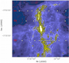 |
Fig. 5 Orion dust opacity map at 850 μm by Lombardi et al. (2014), convolved at an angular resolution of 36′′. Contours are (0.056, 0.24, 0.56, 1.36, and 1.61) × 10−3, which according to Lombardi et al. (2014) correspond to visual extinctions of ~1.3, 5.6, 13.2, 23.8, and 38 mag. Positions observed with the 30m telescope are indicated with triangles. Labels in red indicate the cut IDs. |
3 Observations
The 3 and 2 mm observations were carried out using the IRAM 30-m telescope at Pico Veleta (Spain) during three observing periods in July 2017, August 2017, and February 2018. The observing mode was frequency switching with a frequency throw of 6 MHz well adapted to removing standing waves between the secondary mirror and the receivers. The Eight MIxer Receivers (EMIR) and the Fast Fourier Transform Spectrometers (FTS) with a spectral resolution of 49 kHz were used for these observations. The intensity scale is TMB, which is related to  by
by  (see Table B.1 in Fuente et al. 2019). The difference between
  and TMB is ≈17 % at 86 GHz and 27% at 145 GHz. The uncertainty in the source size is included in the line intensity errors, which are assumed to be ~20%.
For TMC 1 and Barnard 1, we use observations of the CS 1 →0 line carried out with theYebes 40 m radiotelescope (Tercero et al. 2021). The 40 m telescope is equipped with HEMT receivers for the 2.2–50 GHz range, and asuperconductor-insulator-superconductor (SIS) receiver for the 85–116 GHz range. Single-dish observations in K-band (21–25 GHz) and Q-band (41–50 GHz) can be performed simultaneously. The backends consisted of a FFTS covering a bandwidth of ~2 GHz in band K and ~9 GHz in band Q, with a spectral resolution of ~38 kHz. Detailed information about the setups observed in the IRAM 30 m and Yebes 40 m telescopes and the telescopes parameters were presented in Fuente et al. (2019).
4 Physical conditions: molecular hydrogen density
In order to derive the gas physical conditions, we use the line intensities of the observed CS, C34 S, and 13CS lines. CS has been widely used as a density and column density tracer in the interstellar medium (Linke & Goldsmith 1980; Zhou et al. 1989; Tatematsu et al. 1993; Zinchenko et al. 1995; Anglada et al. 1996; Bronfman et al. 1996; Launhardt et al. 1998; Shirley et al. 2003; Bayet et al. 2009; Wu et al. 2010; Zhang et al. 2014; Scourfield et al. 2020). We fit the lines using the molecular excitation and radiative transfer code RADEX (van der Tak et al. 2007), which do not consider local thermodynamic equilibrium (LTE), and the collisional coefficients calculated by Denis-Alpizar et al. (2018). During the fitting process, we fix the ratios 12C/13C = 60 and 32S/34S = 22.5 (Savage et al. 2002; Gratier et al. 2016). Isotopic fractionation is not expected to be important for sulfur. The CS molecule is enriched in 34S at early time because of the 34S+ + CS reaction but not at the characteristic times of dense clouds, which justifies the use of a fixed C34S/CS ratio to derive molecular hydrogen densities and abundances (Loison et al. 2019b). More controversial is the 12CS/13CS ratio; the adopted value is consistent with the results of Gratier et al. (2016) in TMC 1 and Agúndez et al. (2019) in L 483. This value is also consistent with chemical predictions for typical conditions in dark clouds and evolutionary times of approximately a few hundred thousand years (Colzi et al. 2020; Loison et al. 2020). We assume a beam-filling factor of 1 for all transitions (the emission is more extended than the beam size).
In addition, we assume that gas and dust are thermalized, that is, that the kinetic temperature Tk is equal to thedust temperature derived from far-infrared and millimeter observations (TMC 1: Fuente et al. 2019; B 213: Palmeirim et al. 2013; Perseus: Zari et al. 2016; Orion: Lombardi et al. 2014). This assumption might underestimate the gas temperature at the low extinctions where the gas can be heated by the photoelectric effect to temperatures higher than the dust temperature (see, e.g., Okada et al. 2013). In order to test the reliability of this assumption we carried out thermal-balance calculations for three representative cases. Figure 6 shows the dust and the gas temperatures calculated using the Meudon PDR (1.5.4) (Le Petit et al. 2006; Goicoechea & Le Bourlot 2007; Gonzalez Garcia et al. 2008; Le Bourlot et al. 2012). The three panels showthe output for three models that are representative of the physical conditions in Taurus (Fuente et al. 2019; Navarro-Almaida et al. 2020), Perseus (Navarro-Almaida et al. 2020), and Orion. For Orion, we adopt χUV ~ 60, which is the incident Draine field estimated in the Horsehead nebula (Pety et al. 2005; Goicoechea et al. 2006, 2009a,b; Guzmán et al. 2011, 2012a,b, 2013; Le Gal et al. 2017; Rivière-Marichalar et al. 2019). In every case the value of the cosmic ray ionization rate is set to ζ(H2) = 5 × 10⁻¹⁷ s−1. For all cases it could be observed that Tg ~ Td within ~1 K when considering the region with AV > 4 mag. It should be noted that these calculations consider a plane-parallel slab illuminated from one side. In the morerealistic case of a cloud illuminated from the front and back, the visual extinction at which Tg ~ Td would be ~8 mag. In the outer part of the cloud,the gas temperature is higher than the dust temperature by an amount that varies with the incident UV field. Following our calculations, for AV ~ 2 mag, Tg ~ Td + 5 K in Taurus, Tg ~ Td + 10 K in Perseo, and Tg ~ Td + 15 K in Orion. Most of our points are located in the region >8 mag. Moreover, the lines of H13CO+, HC18O+, H13CN, HCS+, and OCS are only detected towards AV > 8 mag. Therefore, we consider that our assumption is reasonable for the goals of this paper, which is focused on statistical trends.
In our calculations, we let n(H2) and N(CS) vary as free parameters and explore their parameter space following the Monte Carlo Markov chain (MCMC) methodology with a Bayesian inference approach. In particular, we used the emcee (Foreman-Mackey et al. 2013) implementation of the Invariant MCMC Ensemble sampler methods by Goodman & Weare (2010). This method was already used in Rivière-Marichalar et al. (2019) and Navarro-Almaida et al. (2020), and allowed us to estimate the density as long as the two transitions of CS, J = 2 →1, and 3 →2 are detected, which reduced the total number of valid spatial points to 244. In TMC 1 and Barnard 1b, we complemented the J = 2 →1 and 3 →2 observations with data of the J = 1 →0 line as observed with the 40 m Yebes telescope. In these two clouds, we were able to estimate densities at the edge of the cloud down to AV = 3 mag, where the J = 3 →2 line of CS is not detected. These estimates were published in Fuente et al. (2019) and Navarro-Almaida et al. (2020), and are included in the present analysis. For the remaining sources, we do not have CS J = 1 →0 data, and we are only sensitive to densities of n(H2) ~ 104 cm−3 or larger. InFig. 7 we plot the derived molecular hydrogen densities as a function of the visual extinction, with colours indicating the different observed filaments. As mentioned above, densities <3 × 103 cm−3 are only measured in TMC 1 and Barnard 1b as a consequence of our methodology and the limitations of our dataset. There is a clear trend of increasing hydrogen density with visual extinction, with higher densities in the inner layers of the clouds. However, the dispersion is large, with values of the molecular hydrogen density varying by a factor of >30 for a given visual extinction. This dispersion remains even if only the points of a given cloud are considered, which suggests that it is not the result of mixing clouds in different environments but the consequence of a complex density structure with different gas layers along the line of sight.
The distribution of the molecular hydrogen densities and gas thermal pressures (n(H2) × TK) obtained forthe 244 points is represented in the top row of Fig. 8, color-coded according to the molecular cloud that they belong to, with legends indicating the mean, median, and standard deviation values of their corresponding distributions in logarithmic units. The densities in Taurus show a peaky distribution with a low mean density value, as expected for low-mass star-forming regions. Perseus has higher values of densities and pressures, with a wider distribution. The highest values of density and pressure and the most flattened distribution is observed in Orion. In order to explore the origin of the wide distribution in Perseus, we made the density and pressure histograms differentiating the individual clouds of this region (middle row in Fig. 8). NGC 1333 and IC 348, with higher temperatures and extinctions, have density and pressure values closer to those of Orion, while low temperature regions such as Barnard 1b, L 1448, and Barnard 5 show values more similar to those obtained in Taurus. The wide distribution shown by Perseus therefore seems to be produced by the different contributions of its five observed regions, comprising a certain range of physical parameters. We carried out the same analysis in Orion, although we only observed three cuts without statistical significance. The three peaks observed in the pressure distribution of Orion (bottom row of Fig. 8) indeed correspond to the three observed cuts. As one would expect, the cut located closer to the Orion nebula (cut 3) is the one with the highest pressure. The cut with the lowest pressure, that is, the most similar to low-mass star forming regions, is the one in OMC 4 (cut 2). The cut in OMC 3 presents intermediate conditions. This plot suggests that the range of physical conditions in high-mass and intermediate-mass star forming regions is wider than the one observed in the low-mass star forming regions, which is surely related to the feedback of the recently formed intermediate- and high-mass stars in the environment.
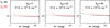 |
Fig. 6 Dust and gas temperature derived using the Meudon PDR 1.5.4 code for a plane-parallel isobaric cloud illuminated from only one side. The plotted dust temperature is a weighted average of the dust temperatures calculated for different grain sizes, assuming a grain size distribution, ngr ∝ a−3.5 (Mathis et al. 1977), where ngr is the number of grains with size a, and the minimum and maximum grain sizes are given by a = 10−7 cm and 3 × 10⁻⁵ cm, respectively. The incident UV flux and thermal pressure of each calculation are indicated in the panels. The values have been selected to represent the physical conditions in Taurus (χUV ~ 5), Perseus (χUV ~ 25), and Orion (χUV ~ 50), where χUV is the incident UV field in units of the Draine field (Draine 1978). |
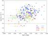 |
Fig. 7 Relation between derived molecular hydrogen densities and visual extinctions for the sample used in this study. Colors indicate the different observed regions as shown in the plot legend. Densities <3 × 103 cm−3 are only measured in TMC 1 and Barnard 1b as a consequence of our methodology and the limitations of our dataset, which is incomplete for the rest of the regions (see text). This value is marked with a dotted horizontal line. |
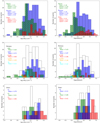 |
Fig. 8 Histograms of the derived molecular hydrogen densities (left column) and corresponding pressures (right column). Histograms comprise values for the whole sample indicating the corresponding molecular complexes (top row), clouds in Perseus (middle row), and cuts of the Orion cloud (bottom row). In the middle and bottom rows, white histograms show the distribution for the molecular cloud complex to facilitate the comparison. Statistical parameters of the different distributions are indicated in each histogram legend. |
5 Molecular column densities
The fitting of the CS (and its isotopologs C34S and 13CS) lines described in Sect. 4 allows us to accurately determine the CS column density values, and therefore its molecular abundances, for each of the 244 points where the MCMC method can be applied. Considering the derived molecular hydrogen densities, we can also determine the molecular column densities and the molecular abundances for a set of species for which only one line is observed: 13CO, C18O, HCO+, H13CO+, HC18O+, H13CN, HNC, HCS+, SO, 34SO, H2S, and OCS. We use the RADEX code and the collisional coefficients included in Table 2. Uncertainties are calculated taking into account the errors in the measurement of the integrated line intensities as well as the systematic errors of 10–20% due to the flux calibration.
In the following, we investigate the relationship between the obtained molecular abundances and the molecular cloud physical parameters: kinetic temperature, extinction, and molecular hydrogen density, considering each molecular cloud separately and the statistical trends observed for the complete dataset. As a first approach, in this section we analyze the correlations and trends that can be observed in the corresponding figures in a qualitative way. A quantitative discussion based on numerical values of correlation coefficients is provided in Sect. 6. It is important to note that inthe particular case of the CS, we obtain the molecular abundance by fitting CS and its isotopologs C34S and 13CS simultaneously, which implies that we are already taking into account the influence of line opacity. We also assume that the CS, C34S, and 13CS line emission comes from the same region. The method applied for the other species is different, as mentioned above, and this should be considered in the interpretation of the results.
5.1 CS
This is a diatomic molecule with well-known collisional coefficients (Denis-Alpizar et al. 2013) and, as already mentioned in Sect. 4, is widely used as a density and column density tracer in the interstellar medium. In our Galaxy, CS is the most ubiquitous sulfur compound, the only one that is commonly detected in photodissociation regions (PDRs; Goicoechea et al. 2016; Rivière-Marichalar et al. 2019) and protoplanetary disks (Dutrey et al. 1997, 2011; Fuente et al. 2010; Guilloteau et al. 2016; Teague et al. 2018; Phuong et al. 2018; Le Gal et al. 2019). Therefore, a complete understanding of its chemistry would be of great value for estimating the physical conditions of the gas and sulfur depletion in many astrophysical environments. In the following, we investigate the behavior of CS abundance in the GEMS sample.
The relationships between the derived CS molecular abundances and the main physical parameters of the clouds (kinetic temperature, extinction, and molecular hydrogen density) are represented in Fig. 9. The rows of the figure represent the same relations but classifying the data following different criteria: first, the molecular cloud to which the points belong, and then dividing the dataset considering bins of temperature, extinction, or density. These divisions allow us to study the possible influence of the variation of these parameters in the whole sample, beyond the particular environment of each cloud. We consider bins of temperature with limits of 15 and 20 K, which approximately describe different trends observed in the plots. Bins of extinction are established below 8 magnitudes (translucentcloud), between 8 and 20 magnitudes (dense core in low-mass star forming regions), and above 20 magnitudes (dense cores in intermediate and massive star-forming regions). Bins of molecular hydrogen density are considered with limits of 4 and 5 in logarithmic scale, which describe the range of values that we observe in our data.
The decreasing linear relation between CS molecular abundance and molecular hydrogen density is very clear. This trend, the linear fittingof which for the whole dataset is included in the top-right panel of Fig. 9, is common to the three molecular clouds, although each cloud presents differentiated physical conditions. Moreover, albeit with a dispersion by a factor of three, this trend remains for almost three orders of magnitude. Therefore, this parameter is the main driver of the changes in the CS abundance in our sample.
In Fig. 9, we also show X(CS) as a function of the gas kinetic temperature. A possible correlation is observed between X(CS) and Tk up to ~14 K. Afterwards the abundance decreases with temperature in the range Tk ~14−20 K. Beyond this point, Tk > 20 K, the scatter increases and no clear trend is observed. Interestingly enough, the classification of points according to their molecular cloud precisely reproduces this behavior: points with Tk < 14 K belong to Taurus and the low-temperature regions of Perseus, L1448 and B1B. In these cuts, X(CS) is increasing with Tk. It should be noted that density and Tk are anti-correlated in these regions, with the lowest values of Tk being associated with the highest densities. This trend with Tk is then related with the overall trend of X(CS) decreasing with n(H2). On the other hand, most of the Perseus points show the decreasing relation between 15 and 20 K. We interpret this behavior as the consequenceof the CS photodissociation at the illuminated cloud edge. We remind that G0 is higher in star forming regions of Perseus than in Taurus (Navarro-Almaida et al. 2020) and in our sample of starless cores, the highest temperatures are found at the lowest visual extinctions. Lastly, points belonging to Orion show a high scatter and no clear trend with temperature. Interestingly, the Orion points follow the general anti-correlation between X(CS) and gas density quite well, confirming density as the dominant parameter of the CS chemistry.
The depletion of CS has been widely studied in starless cores, and the X(CS)/X(N2H+) abundance ratio has been proposed as an evolutionary diagnostic for these objects (Tafalla et al. 2002, 2004; Tafalla & Santiago 2004; Hirota & Yamamoto 2006; Heithausen et al. 2008; Kim et al. 2020). Our data show that the CS abundance decreases almost linearly with the density for almost three orders of magnitude. Moreover, this trend remains valid for regions regardless of the star formation activity of the region, providing a tool with which to predict density and to subsequently interpret molecular observations in large scale surveys. However, we must keep in mind that our cuts avoid protostars and the hot cores or hot corinos, bipolar outflows, and HII regions formed around them. The binding energy of CS is estimated to be ~3200 ± 960 K (Wakelam et al. 2017), and therefore thermal evaporation is expected to be efficient when the dust temperature is >50 K. Sputtering is also efficient as a mechanism to release molecules to the gas phase for shock velocities >10 km s−1 (Jiménez-Serra et al. 2008). Therefore, high CS abundances are expected in hot cores/corinos and bipolar outflows where the icy mantles are eroded (Bachiller & Pérez Gutiérrez 1997; Jiménez-Serra et al. 2008; Esplugues et al. 2014; Crockett et al. 2014).
References for the collisional rate coefficients used for the volume density estimates.
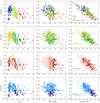 |
Fig. 9 Relation of the CS molecular abundance to cloud physical parameters: kinetic temperature (left column), extinction (middle column), and molecular hydrogen density (right column). From top to bottom, the dataset is color-coded according to the molecular cloud of the points (first row), bins of kinetic temperature (second row), bins of extinction (third row), and bins of molecular hydrogen density (last row), as indicated in the corresponding legends. The black line in the top right plot shows the linear correlation between X(CS) and n(H2) for the whole sample, with the correlation parameters indicated in the legend. |
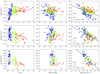 |
Fig. 10 Relation of the HCO+ (top row), H13CO+ (middle row), and HC18O+ (bottom row) molecular abundances to cloud physical parameters: kinetic temperature (left column), extinction (middle column), and molecular hydrogen density (right column). The dataset is color-coded according to the molecular cloud of the points, as indicated in the legends. The black lines show the linear correlations between molecular abundances and molecular hydrogen density for the corresponding whole samples, with the correlation parameters indicated in the legends. |
5.2 HCO+, H13CO+, HC18O+
We derived the molecular abundances of HCO+, H13CO+, and HC18O+ from the observations of their J = 1 →0 rotational line. Isotopic 12C/13C and 16O/18O fractionation has been predicted under the physical conditions prevailing in molecular clouds for HCO+ (Roueff et al. 2015; Loison et al. 2019b, 2020; Colzi et al. 2020). For this reason, we prefer to independently fit the three isotopologs. The number of detections depends on the abundance of each isotopolog. The number of positions with AV < 8 mag detected in HCO+ 1 →0 is significantly larger than those detected in H13CO+ 1 →0 (see Fig. 10). The HC18O+ 1 →0 line is only detected for AV >8 mag. Thus, the observation of the three isotopologs allows us to probe different regions of the cloud.
We explore the possible (anti-)correlations of the abundances of these ions with kinetic temperature, extinction, and molecular hydrogen density in Fig. 10. The abundance of the main isotopolog, X(HCO+), seems to increase with temperature. This apparent correlation is the consequence of the fact that the HCO+ 1 →0 line is optically thick. In this regime, line intensities simply reflect the excitation temperature in the layer with τ ~ 1, and our calculations only provide a lower limit to the real HCO+ abundance. Moreover, this line is self-absorbed in many positions, especially in Taurus (Fuente et al. 2019). This apparent correlation disappears for the less abundant isotopologs, H13CO+ and HC18O+, whose emission is expected to be optically thin. These isotopologs can be used as proxies for HCO+. Figure 10 shows the decrease in the abundance of these molecular ions with density. This anti-correlation is particularly clear for HC18O+, that is, for the inner layers of the gas, as we only detect this molecule for AV > 8 mag.
In Fig. 11 we show N(HCO+)/N(H13CO+) and N(H13CO+)/N(HC18O+) as derived from their J = 1 →0 spectra. We obtain N(H13CO+)/N(HC18O+) ≈ 10−25, which is consistent with our assumption that the emission of these species is optically thin. It should be noted that the values of N(H13CO+)/N(HC18O+) are higher than approximately 10 for most positions, with an average value of about 15. This value is higher than that expected when taking into account the adopted 12C/13C and 16O/18O isotopic ratios. One reason is the presence of several velocity components at many of the observed positions. Only the most intense of these components is detected in N(HC18O+), which introduces uncertainties of a factor of two in the measured N(H13CO+)/N(HC18O+) ratio. Carbon isotopic fractionation could also explain the high values of the N(H13CO+)/N(HC18O+) ratio. Chemical models predict that the HCO+/H13CO+ abundance ratio varies during cloud evolution and could be <60 for ages of a few 0.1 to ~1 Myr for typical conditions in dark clouds (Roueff et al. 2015; Colzi et al. 2020; Loison et al. 2020). The overabundance of H13CO+ could pushthe N(H13CO+)/N(HC18O+) to values around >10.
The N(HCO+)/N(H13CO+) ratio correlates with the gas temperature and is lower than the 12C/13C isotopic ratio at all positions except a few points in Orion and Perseus. This strongly supports the interpretation that the HCO+ 1 →0 line is optically thick at all the positions in which H13CO+ is detected. The obtained values of N(HCO+) are only reliable at low visual extinction (AV < 5 mag). At these low extinctions, we measured X(HCO+) ~10−10−3 × 10⁻⁹. The HCO+ abundance in the diffuse medium has been estimated to be N(HCO+)/N(H2) = 3 × 10⁻⁹ (Liszt et al. 2010; Liszt & Gerin 2016), which is coincident with the upper end of our range.
The abundance ratio N(HCO+)/N(CO) is traditionally used to estimate the ionization degree, X(e−), in molecular clouds (Wootten et al. 1979; Guelin et al. 1982; Caselli et al. 1998; Zinchenko et al. 2009; Fuente et al. 2016, 2019). For regions where CO is not heavily depleted (constant CO abundance), X(HCO+) ∝  (see e.g., Caselli et al. 1998). If we assume that the cosmic ray molecular hydrogen ionization rate, ζ(H2), remains constant for the visual extinctions AV > 8 mag probed with our HC18O+ data, the correlation found between HC18O+ and n(H2) is consistent with X(e−) ∝ n−0.5, which agrees with chemical predictions for starless cores (Caselli et al. 1998). However, it should be noted that the Orion points lie systematically below the straight line fitted in Fig. 10 while positions in Taurus are systematically above this line. Although suggestive of a different X(e −), a multitransition study of HCO+ and its isotopologs and chemical modeling are required to establish firm conclusions. A combination of uncertainties in n(H2) in the low-density positions in Taurus and opacity effects due to the higher extinction towards the high-density positions towards Orion could also produce this effect.
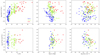 |
Fig. 11 Relation of the HCO+/H13CO+ (top row) and H13CO+/HC18O+ (bottom row) molecular abundance ratios to cloud physical parameters: kinetic temperature (left), extinction (middle), and molecular hydrogen density (right). The dataset is color-coded according to the molecular cloud of the points, as indicated in the legend. |
5.3 HCN, H13CN, HNC
The isomers hydrogen cyanide (HCN) and hydrogen isocyanide (HNC) are widely observed in the interstellar medium. They have been detected in diffuse clouds (Liszt & Lucas 2001), translucent molecular clouds (Turner et al. 1997), dark cloud cores (Hirota et al. 1998; Hily-Blant et al. 2010), and in low-mass and massive star-forming regions (Colzi et al. 2018; Goicoechea et al. 2019; Hacar et al. 2020; Le Gal et al. 2020). Understanding their chemical behavior in all these environments is crucial for the correct interpretation of molecular observations. Figure 12 shows the relationships between HCN and H13CN molecular abundances and the physical parameters of the gas, classifying the data as a function of the hosting molecular cloud. The HCN column density was derived from the total area of the 1 →0 line (summing up of the hyperfine components) and assuming the same physical conditions as above. The HCN 1 →0 line is optically thick in almost allpositions with AV > 8 mag. Moreover, the profile of the main hyperfine component presents deep self-absorption features towards the Taurus dark cores (see Fuente et al. 2019). This is the reason for the apparent low HCN abundance in Taurus positions. This kind of self-absorbed profile is less common in Perseus and does not appear in our limited sample of positions in Orion.
In order to avoid opacity and self-absorption effects, we prefer to trace the behavior of this molecule using its isotopolog, H13CN. We are aware that fractionation might be important for HCN and that the HCN/H13CN ratio can vary by a factor of about two (Roueff et al. 2015; Zeng et al. 2017; Loison et al. 2019a, 2020; Colzi et al. 2020). Thus, H13CN is a good proxy for HCN with an uncertainty of a factor of two. The H13CN 1 →0 line is only detected in positions with AV > 8 mag (see Fig. 12). We observe a strong anti-correlation between the molecular abundance and H2 density, with less scatter than in the case of H13CO+ and HC18O+. The trend iscommon to the three molecular clouds, and remains for around two orders of magnitude in density. This similarity between HCO+ and HCN isotopologs suggests a related chemistry in dark clouds. The recombination of protonated compound HCNH+ is the most important formation mechanism for HCN and HNC in cold dark clouds (Loison et al. 2014). The radical CN is also a product of this recombination which itself can react with H to produce HCN+ which is rapidly recycled to HCNH+ by reactions with H2. The abundance of these isomers is therefore sensitive to variations in the gas ionization degree and H
 abundance, similarly to the case of the molecular ions H13CO+ and HC18O+. Zinchenko et al. (2009) carried out a survey of HN13C and H13CN in massive star forming regions, and found an anti-correlation between the HN13C abundance and the gas ionization degree. However, they did not obtain the same result for H13CN. In contrast to HNC, the HCN abundance is boosted in the shocked gas associated to bipolar outflows and the hot cores in the early stages of massive star formation (Schilke et al. 1992; Schöier et al. 2002; Rolffs et al. 2011; James et al. 2020; Hacar et al. 2020). Our data show that the H13CN abundance decreases with n(H2) in the quiescent gas. Hily-Blant et al. (2010) studied the chemistry of HCN, HNC, and CN in starless cores, deriving X(H13CN) ~ 10−11 towards the millimeter emission peaks. These values are in good agreement with the values we obtained for densities n(H2) > 105 cm−3, in the lower end of the observed range of H13CN fractional abundances.
It is interesting to compare the behavior of X(H13CN) with that of X(HNC), whose relationships with cloud physical parameters are also plotted in Fig. 12. X(HNC) also presents a decreasing abundance with molecular hydrogen density, but with a shallower power law of slope approximately −0.5. This could be mainly due to the opacity, because the HNC line is expected to be optically thick in dense cores. This shallow slope is also observed in the X(HCN) versus n(H2) correlation.
The HCN/HNC line ratio has been proposed as a direct probe of the gas kinetic temperature (e.g., Goldsmith et al. 1981, 1986; Baan et al. 2008; Hacar et al. 2020), with increasing values of this ratio probing warmer material, which could lead to it being used as a new chemical thermometer of the molecular interstellar medium. In order to explore this proposal, Fig. 13 shows the relationships between the HCN/HNC and H13CN/HNC line ratios with kinetic temperature. In our case, the lack of reliability of derived HCN abundances due to the mentioned self-absorption effects in Taurus and partially in Perseus prevents a reliable analysis of the trends found in these clouds. On the other hand, Orion points indeed show slight increase in this line ratio with temperature, in good agreement with results by Hacar et al. (2020), but the number of points is not high enough to give a statistically robust conclusion. The observed trend for Orion points disappears when considering the H13CN/HNC line ratio. Indeed, considering all the points (Taurus, Perseus and Orion), the H13CN/HNC ratio seems to decrease. Again, we think that this is not real, and is the effect of the high optical depths of the HNC J = 1 →0 line in cold cores (see, e.g., Daniel et al. 2013), which lead to an underestimation of N(HNC). Multi-transition observations of HCN, HNC, and their isotopologs H13CN and HN13C are requiredto constrain the X(HCN)/X(HNC) ratio. A deeper analysis based on chemical models and 3D radiative transfer calculations should be carried out in order to determine the behavior of this abundance ratio with kinetic temperature.
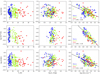 |
Fig. 12 Relation of the HCN (top row), H13CN (middle row), and HNC (bottom row) molecular abundances to cloud physical parameters: kinetic temperature (left), extinction (middle), and molecular hydrogen density (right). The dataset is color-coded according to the molecular cloud of thepoints, as indicated in the legend. Black lines show the linear correlations between molecular abundances and molecular hydrogen density for the corresponding whole samples, with the correlation parameters indicated in the legends. |
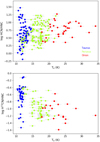 |
Fig. 13 Relation of the HCN/HNC (top) and H13CN/HNC (bottom) line ratios to kinetic temperature. The dataset is color-coded considering the molecular cloud of the points, as indicated in the legend. |
5.4 H2S
Knowledge of the H2S molecule is key to understanding sulfur chemistry. Sulfur is one of the most abundant elements in the Universe, and its presence in the interstellar medium has been widely studied. Sulfur atoms in interstellar ice mantles are expected to preferentially form H2S because of the high hydrogen abundances and the mobility of hydrogen in the ice matrix. Therefore, studying H2S abundance in the gas phase is essential to our understanding of the chemical processes that lead to sulfur depletion in these environments. Of particular importance, this molecule was the subject of a previous paper of the GEMS series, where the H2S observations of TMC 1-Cand Barnard 1b were analyzed (Navarro-Almaida et al. 2020). In Navarro-Almaida et al. (2020) we estimated the o-H2S abundance using the ortho-H2O collisional coefficients calculated by Dubernet et al. (2009), scaled to ortho-H2S. Here we use the specific o-H2S collisional coefficients with o-H2 and p-H2 recently calculated by Dagdigian (2020). The difference between these two sets of collisional coefficients is of a factor of ~1.7 at 10 K in collisions with p-H2, which implies that the re-estimated ortho-H2S column densities in TMC 1 and B1b are a factor of ~1.7 lower than those reported by Navarro-Almaida et al. (2020). This moderate factor is within the usual uncertainties of column density estimates and does not affect any of the conclusions of this paper. The ortho-H2S abundances derived from the observations of the  = 11,0 → 10,1 line are shown in Fig. 14. These abundances are represented as a function of the gas physical parameters, and the points are classified according to their molecular clouds. We also observe in this case a strong anti-correlation between H2S abundance and molecular hydrogen density, spanning over around three orders of magnitude. Interestingly, we do observe a displacement between the trend of the points belonging to Taurus and that shown by the warmer Perseus and Orion. This behavior was already observed by Navarro-Almaida et al. (2020) based on the analysis of the data towards TMC 1-C and Barnard B1b. The analysis of the whole sample confirms and extends this behavior, with the observed positions in Taurus following a steeper law with density than those in Perseus and Orion. Navarro-Almaida et al. (2020) explained this behavior as the consequence of the different chemical desorption efficiency in bare and ice-coated grains.
Simultaneously with H2S, we observed the H S
S  = 11,0 → 10,1 line with very few detections, which proves the low optical depth of the same line of the main isotopolog. Optical depth effects are therefore not expected to bias the (anti-)correlation with density.
5.5 SO, 34SO
One of the most abundant and easily observable species is SO which, along with CS, is the most abundant S-bearing molecule in the gas phase. Within GEMS, we observed the SO JN = 22 → 11, 23 → 12, 32 → 21, 34 → 23, and 44 → 33 lines, allowing a multi-transition study. However, in most positions we only detected one or two of the observed lines. In order to apply a uniform analysis method to all the positions included in this statistical analysis, we estimated the SO column density based on the intensities of the SO JN 22 → 11 line, assuming the molecular hydrogen density estimated from CS. In addition to the main isotopolog, we observed the JN = 23 → 12 line of the rarer isotopolog 34SO which can provide important information with which to constrain the SO abundance in the most obscured regions.
The relations between SO and 34SO molecular abundances and gas physical parameters are shown in Fig. 15, with points classified as a function of their molecular clouds. As in previous cases, a linear decreasing relation with molecular hydrogen density is found in both cases, but for SO isotopologs the relation seems to be weaker and with a wider scatter. In order to explore the origin of this scatter, we plot the relationship between SO molecular abundance and n(H2) in Fig. 16, with points classified according to bins of extinction, and the corresponding linear relations existing for each case. We observe that the slope is similar for all ranges of extinction, but the intercept changes, being lower for AV < 8 mag. This suggests that the abundance of SO is lower in the outer part of the cloud, more likely because of the enhanced UV radiation.
There are some positions with high N(SO)/N(34SO) (>50), and most of these positions are in Orion. We do not expect isotopic fractionation for 32S/34S. Therefore, we discuss some observational uncertainties. First of all, many positions of the cut Ori-C2-1 present two velocity components in the SO line. Only the most intense of these components are detected in 34SO. As we did not carry out a differentiated study for each velocity component, N(SO)/N(34SO) is expected to be overestimated towards these positions. However, it is difficult to justify N(SO)/N(34SO) > 50 based only on this effect. We recall that we assume the same physical conditions for SO and 34SO. A steep gradient in temperature and density along the line of sight could also induce anomalously high N(SO)/N(34SO) ratios.
5.6 HCS+, OCS
The S-bearing species HCS+ and OCS are detected only in a fraction of the observed positions, meaning lower statistical significance. Nevertheless, we consider that it is interesting to include them in our study. Figure 17 shows the relation between the HCS+ and OCS molecular abundances and the physical parameters of the clouds. Both species are only detected for extinctions greater than ~8 mag, and OCS is only detected in Taurus and Perseus, but not in Orion. Based on our data, we derive X(OCS) < 4 × 10⁻¹⁰ in Ori-C1-2, X(OCS) < 1 × 10⁻⁹ in Ori-C2-2, and X(OCS) < 5 × 10⁻¹⁰ in Ori-C1-3,which are the extinction peaks of the three cuts observed in Orion. These upper limits are in the range of OCS abundances derived in Perseus and Taurus. Therefore, the nondetection might be the consequence of the limited sensitivity of the Orion observations.
HCS+ is the protonated species of CS and its precursor in diffuse clouds and the external layers of the photon-dissociation region (Sternberg & Dalgarno 1995; Lucas & Liszt 2002; Rivière-Marichalar et al. 2019). Contrary to HCO+, deeper into the molecular cloud HCS+ is rapidly destroyed by reaction with O, and CS is formed by neutral–neutral reactions such as SO + C → CS +O. In agreement with its origin in the outer layers of molecular clouds, in Fig. 17 we observe a steep decrease of the HCS+ with visual extinction. In fact, contrary to most of the species studied, the (anti-)correlation of X(HCS+) with AV presents less scattering than its relationship with gas density. In the case of OCS, we do not find any clear relation between its abundance and the physical conditions of the clouds. This is most likely due to the small number of detections, which does not allow us to properly cover the parameter space of our study.
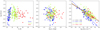 |
Fig. 14 Relation of the H2S molecular abundance to cloud physical parameters: kinetic temperature (left), extinction (middle), and molecular hydrogen density (right). The dataset is color-coded according to the molecular cloud of the points, as indicated in the legend. Lines in the right plot show the linear correlations between X(H2S) and n(H2) for the whole sample, in black, and for each one of the molecular clouds, color-coded as in the points. The corresponding correlation parameters are indicated in the legend. |
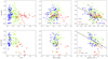 |
Fig. 15 Relation of the SO (top row) and 34SO (bottom row) molecular abundances to cloud physical parameters: kinetic temperature (left), extinction (middle), and molecular hydrogen density (right). The dataset is color-coded according to the molecular cloud of the points, as indicated in the legend. Black lines show the linear correlations between molecular abundances and molecular hydrogen density for the corresponding whole samples, with the correlation parameters indicated in the legends. |
5.7 13CO, C18O
We derived the 13CO and C18O abundances from the observationsof their J = 1 →0 rotational lines. The major uncertainties in our calculations come from opacity effects in the studied lines and the assumption that gas and dust share the same temperature. Assuming a standard CO abundance, X(CO) ~8 × 10⁻⁵, and the same isotopic ratios as in previous sections, the 13CO 1 →0 and C18O 1 →0 lines are expected to be optically thin for AV < 8−10 mag and AV < 60−100 mag respectively. Therefore the estimated C18O abundances are reliable in almost the entire range of visual extinctions considered in our study, with the exception of a few positions with AV > 60 mag that have been removed from the plots and are not considered in this section hereafter. The second approximation is our assumption that Td = Tgas. As mentioned in Sect. 4, this approximation is reasonable for well-shielded regions of molecular clouds, AV > 8 mag (see also Roueff et al. 2021), where the 13CO 1 →0 line is expected to be optically thick; however,it is inaccurate at the cloud edges, where UV photons heat the gas more efficiently than the dust by the photoelectric ejection of electrons from grains and polycyclic aromatic hydrocarbons (PAHs). Caution should be taken in sources bathed in enhanced UV fields, like Orion and IC 348, where the gas temperature is ~15 K higher than the dust temperature in the cloud surface. In order to estimate the error due to the uncertainty in the gas temperature in these regions, we carried out a simple calculation assuming typical physical values of n(H2) = 104 cm−3 and N(13CO) ~ a few 1015 cm−2. The difference in the derived N(13CO) assuming temperatures of between 15 and 30 K is of ~20%. Our approximation is better for Taurus, where the incident UV field is low and gas and dust temperature agree within <5 K even in the more external layers (see Fig. 6).
The relationship between the derived abundances and the physical parameters of the clouds is represented in Fig. 18, where the positions of Taurus, Perseus, and Orion are represented in different panels. Points belonging to Taurus show clear trends with temperature and visual extinction, and a poorer correlation with density. The 13CO abundance increases with visual extinction until AV ~ 3 mag; for AV > 3 mag, the 13CO abundance is decreasing with visual extinction. As mentioned above, the 13CO line is expected to be optically thick for AV > 8 mag, and the calculated 13CO abundance could be underestimated. For AV > 8 mag, the C18O isotopolog is a better proxy for CO. The abundance peak of C18O is found at AV ~5 mag, that is, shifted with respect to the position of the X(13CO) peak. For AV > 5 mag, we observe a decreasing trend in the C18O abundance with visual extinction, although the scatter is wider than in 13CO. The shift between the abundance peak of 13CO and C18O is not due to optical depth effects but to an increase of the N(13CO)/N(C18O) ratio at AV < 5 mag. This offset between the two isotopologs was already observed by Cernicharo & Guelin (1987) and Fuente et al. (2019), and was interpreted as a consequence of the selective photodissociation and isotopic fractionation (Fuente et al. 2019).
There is a tight correlation between X(13CO) and X(C18O) with temperature in Taurus. We observe an increasing relation between the abundances of these species with the gas kinetic temperature until TK ~14 K for 13CO and until TK ~ 12−13 K in the case of C18O, and a decrease in the abundances for higher temperatures. In Taurus, the positions with TK > 14 K correspond to the outer layers of the cloud, where the molecules are photo-dissociated.We measure X(C18O) = (1−5) × 10−8 in the coldest cores.
In Perseus we observe the same trends as in Taurus but with a wider scatter. Peaks of the observed distributions for both 13CO and C18O are found at larger extinctions than in the case of Taurus (AV ~ 7 mag for 13CO and AV ~ 10 mag for C18O), which is expected because the ambient UV field in Perseus is higher than in Taurus. Indeed, based on the Herschel dust temperature and extinction maps, Navarro-Almaida et al. (2020) estimated χUV ~24 for Barnard 1b, which is located in a moderately active star-forming region in Perseus (Hatchell et al. 2007b,a).
We do not detect any clear trend in the Orion positions. It should be noted that dust temperatures are >15 K towards all positions in Orion. Nevertheless, the X(C18O) < 10−7 towards some positions, supporting the interpretation that part of the CO might remain locked in grains for warmer temperatures. Cazaux et al. (2017) analyzed the CO depletion from a microscopic point of view, finding that the CO molecules depleted on grain surfaces show a wide range of binding energies, from 300 to 830 K (Tevap ~15−30 K), depending on the conditions (monolayer or multilayer regime) in which CO has been deposited. Low abundances of C18O have also been found in the dense and warm inner regions of protostellar envelopes Y"i"ld"i"z et al. (2010); Fuente et al. (2012); Anderl et al. (2016), where complex organic chemistry is going on. In general, we observe larger scatter in the correlations of X(13CO) and X(C18O) with the physical parameters in Orion than in Taurus and Perseus. The complex structure of this giant molecular cloud and the fact that it is located further than Perseus and Taurus produce a mix of regions with different physical conditions along the line of sight and within the beam of the 30 m, increasing the scattering in the estimated abundances. Moreover, our approximation of deriving the molecular abundances assuming a single density and temperature is more uncertain.
Figure 19 represents the relations between N(13CO)/N(C18O) and the gas physical parameters. In accordance with discussions above, we observe a decreasing relation between this ratio and extinction in the case of Taurus points, which can be understood as the consequence of an increase in the 13CO 1 →0 line opacity with visual extinction. This trend is also reproduced in Perseus. Orion, on the other hand, does not show a significant trend along the selected cuts. The mean values of N(13CO)/N(C18O) are 10.9 ± 7.5 in Taurus, 17.3 ± 11.5 in Perseus, and 23.7 ± 10.4 in Orion, i.e., higher in Orion than in Perseus and Taurus.
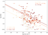 |
Fig. 16 Relation of the SO molecular abundance to the molecular hydrogen density. The dataset is color-coded considering bins of extinction, as indicated in the legend. Lines show the linear correlations between molecular abundances and molecular hydrogen density for each extinction bin, with the correlation parameters indicated in the legend. |
6 Statistical correlations
In this section, we analyze the statistical trends shown in the dataset in a quantitative and uniform way. In order to assess the degree of correlation observed between different parameters, we use the Pearson, Spearman, and Kendall correlation coefficients for the relations between the different parameters considered. These coefficients vary between values of +1 and −1, where the value indicates the strength of the relationship between the variables (± 1 for a perfectdegree of correlation and 0 for unrelated variables), and the sign indicates the direction of the relationship (positive for correlation and negative for anticorrelation). Pearson coefficient is the most widely used correlation parameter to measure the degree of linear relationship between variables. On the other hand, Spearman and Kendall coefficients measure the existence of a monotonic, not necessarily linear, relationship between variables. The Kendall coefficient is usually more robust and is the most used in the case of small samples, but both are based on the same assumptions and provide useful information. Along with the coefficient value, the probability of the null hypothesis (no relation between variables) is also computed, indicating the strength of the result provided by the coefficient. Values for the probability of the null hypothesis higher than 0.001 are considered to indicate no relation at all. We consider the existence of a linear correlation between the corresponding magnitudes when the Pearson correlation coefficient is greater than or similar to ~0.5 in absolute value, and a confirmed strong linear correlation when it is greater than or similar to ~0.7 in absolute value. The relation is confirmed using the Spearman and Kendall coefficients as a further test: in the case of a linear relation, thePearson and Spearman coefficients are similar and in good agreement with the Kendall coefficient, although the latter is systematically smaller in absolute value. Furthermore, a significantly greater value of the Spearman coefficient with respect to the Pearson coefficient in a particular case may indicate, if in good agreement with the corresponding Kendall coefficient, the existence of a nonlinear correlation.
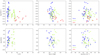 |
Fig. 17 Relation of the HCS+ (top row) and OCS (bottom row) molecular abundances to cloud physical parameters: kinetic temperature (left), extinction (middle), and molecular hydrogen density (right). The dataset is color-coded according to the molecular cloud of the points, as indicated in the legend. |
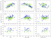 |
Fig. 18 Relation of the 13CO (blue) and C18O (green, multiplied by a factor of ten) molecular abundances to cloud physical parameters: kinetic temperature (left), extinction (middle), and molecular hydrogen density (right), for the three observed molecular clouds, Taurus (top row), Perseus (middle row), and Orion (bottom row). |
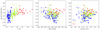 |
Fig. 19 Relation of the 13CO/C18O molecular abundance ratio to cloud physical parameters: kinetic temperature (left), extinction (middle), and molecular hydrogen density (right). The dataset is color-coded considering the molecular cloud of the points, as indicated in the right-hand box. |
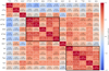 |
Fig. 20 Pearson correlation coefficients of the relations between the molecular abundances of the studied species. Numbers in brackets correspond to the null hypothesis probability in each case, i.e. probability of no relation between variables, where a value higher than 0.001 is considered to indicate no relation at all. Black rectangles indicate groups of molecules with strong correlations (see text). |
6.1 Relations between molecules
We explore the existence of behavioral similarities between the studied molecules by analyzing the relations between their derived molecular abundances. Figure 20 includes the computed Pearson coefficients for these relations. Inthis case, we do not include the Spearman and Kendall coefficients because the obtained relations are all linear and these coefficients do not significantly deviate from the Pearson coefficient value, and therefore do not provide additional information. Some strong correlations between groups of molecules are observed, as indicatedin Fig. 20. In the first place, there is an almost complete correlation between H13CO+ and HC18O+, which is the expected behavior for isotopologs and confirms the results observed in Fig. 11. These molecular ions also correlate with H13CN and HNC, and to a lesser extent with CS and HCS+. It should be noted that HCN is not strongly correlated with H13CN, which is a consequence of the high optical depth and the strong self-absorption features in the HCN 1 →0 spectra. As discussed in Sect. 5, the abundances of all these species steeply decrease with molecular hydrogen density. We propose molecular depletion on the grain surfaces and variations in the gas ionization degree as the causes of this behavior. Indeed, the protonated compounds HCO+ and HCS+ are rapidly destroyed by recombination with electrons to give back the neutral species, CO and CS. On the other hand, the neutral compound HCN is efficiently formed in dark clouds by the dissociative recombination of HCNH+. These three latter ionic species are sensitive to the depletion on the grain surfaces of the neutral compounds, CO, CS, and HCN, respectively, but also to variationsin X(e−). In the absence of shocks and UV photons, cosmic rays are the main ionization agent. Cosmic rays are attenuated with NH within the molecular cloud following a power law whose index is dependent on the propagation mechanism, which itself depends on the turbulence and ion density along the cloud (see, e.g., recent review by Padovani et al. 2020).
A strong grid of correlations is also observed between CS, SO, 34SO, H2S, and OCS, that is, all the S-bearing molecules with the exception of HCS+. The chemistry leading to CS and HCS+ is thought to be initiated by reactions of S+ and neutral compounds in the external layers of the cloud. However, in dark molecular clouds the formation of SO and OCS is initiated by reactions of atomic S with O2 and OH, while CS is partly formed by the reaction C + SO → CS + O (Bulut et al. 2021). The decrease of CS, SO, 34SO, and OCS with density is more likely related with the adsorption of sulfur atoms on the grains surface (Vidal et al. 2017; Laas & Caselli 2019; Navarro-Almaida et al. 2020). In order to estimate how sulfur depletion changes with density, we added the abundances of CS, SO, H2S, and OCS, and found that X(S-bearing) decreases with density following the power law X(S-bearing) ∝ n−0.6 ± 0.1. As the abundances of these species correlate almost linearly with the gas-phase elemental sulfur abundance (see e.g., Vidal et al. 2017), this would imply that sulfur depletion from the gas phase increases by a factor of ~100 in the n(H2) = 103−106 cm−3 range.
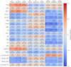 |
Fig. 21 Pearson, Spearman, and Kendall correlation parameters of the relations between the molecular abundances of the studied species (and their ratios) and the molecular cloud physical parameters: kinetic temperature, extinction, and molecular hydrogen density. Numbers in brackets correspond to the null hypothesis probability in each case, i.e. probability of no relation between variables, where a value higher than 0.001 is considered to indicate no relation at all. |
6.2 Relation to Tk and AV
The Pearson, Spearman, and Kendall correlation coefficients for the relations of molecular abundances and a set of selected abundance ratios with the cloud physical parameters (kinetic temperature, extinction, and molecular hydrogen density) are included in Fig. 21. The three first columns of Fig. 21 show the degree of correlation existing between the molecular abundances and the gas kinetic temperature. Correlation coefficients indicate a positive relation between the molecular abundances of 13CO and HCO+ and Tk. The Spearman coefficient is larger than the Pearson one in both cases, pointing to a nonlinear relationship between parameters. This possible correlation becomes weaker for C18O and completely disappears for H13CO+ and HC18O+. This suggests that the correlation of the abundance of 13CO and HCO+ with Tk is not real, but it is an artifact produced by the large opacity of the observed lines in most positions. This could also partially explain the good correlation of X(13CO)/X(C18O) with gas kinetic temperature. However, it is known that this abundance ratio increases with the local UV field, which is known to be correlated with the dust temperature (see e.g., Bron et al. 2018; Fuente et al. 2019). This is corroborated by our observations, from which we obtain that the X(13CO)/X(C18O) ratio is higher in Orion than in Perseus, and is higher in Perseus than in Taurus, when comparing positions located at the same visual extinction, even for AV < 10 mag (see central panel of Fig. 19).
For several other molecules (H13CO+, HC18O+, H13CN, HNC, CS, HCS+, SO, 34SO) the correlation coefficients in Fig. 21 indicate the existence of a weak anti-correlation between molecular abundance and Tk. Confirmation of this trend requires a more detailed analysis. Finally, we do detect significant anti-correlation between H13CO+/13CO and HC18O+/C18O and the gas temperature. This effect is also shown in Fig. 10, where the positions belonging to Orion present lower H13CO+ and HC18O+ abundances than those in Perseus, and the positions belonging to Perseus present lower H13CO+ and HC18O+ abundances than those in Taurus. Indeed, this anti-correlation reflects the different mean abundances of these ions in Taurus, Perseus, and Orion.
Figure 21 reveals that there are no clear relations between the complete datasets of molecular abundances and the extinction. The specific analysis of some molecules in Sect. 5 shows that extinction has indeed an influence in some particular aspects of the molecular abundance behavior, as is seen in the case of SO, 34SO (Sect. 5.5), and mainly 13CO, C18O (Sect. 5.7). However, this influence does not follow a monotonic law. We would like to recall the dependence of the 13CO and C18O abundances on visual extinction in Taurus. The correlation is positive for low visual extinctions and negative for high visual extinctions (see Fig. 18), thus preventing a clean result when considering the whole dataset.
6.3 Relation to n(H2)
The qualitative analysis of the relations between the molecular abundances of the studied species and the gas physical parameters carried out in Sect. 5 already indicated that the molecular hydrogen density is the main driver of the abundance evolution within molecular clouds. This is confirmed by the correlation coefficients in Fig. 21, pointing to clear anti-correlations between most of the molecular abundances and the molecular hydrogen density. Pearson coefficients are greater than or similar to 0.5 in absolute value for HCO+, H13CO+, HC18O+, H13CN, HNC, CS, H2S, SO, and 34SO, and the anti-correlation is particularly strong for HC18O+, H13CN, CS, and H2S, with Pearson coefficients greater than or similar to 0.7. The extremely low values of the probability of the null hypothesis obtained for all these coefficients (at least smaller than 1.0 × 10⁻⁶) testify to the reliability of our results. The correlation stands for densities ranging from n(H2) ~103 cm−3 to ~106 cm−3, i.e., over three orders of magnitude.
In order to gain deeper insight into these relations, we explored the possible dependence of these anti-correlations on visual extinction and star formation activity. The Pearson coefficients of the relations between molecular abundances and n(H2) considering each one of the clouds, as well as dividing the whole sample applying extinction bins of AV < 8, 8−20 mag, and >20 mag, are included in Fig. 22. It can be observed that the correlation with density is always stronger in the case of the Taurus cloud. This is explained by the low incident UV field, turbulence, and gas temperatureprevailing in Taurus, where the chemistry is driven by the freeze-out of molecules on the grain surfaces and ζ(H2). Perseus and Orion show weaker anti-correlations with H2 density, with smaller correlation parameters. However, we do recover strong anti-correlations with density for bins with 8−20 mag in Perseus and >20 mag in Orion. In these deep layers of the Perseus and Orion molecular clouds the gas chemistry is determined by the molecular hydrogen density, as in Taurus. This is a chemical footprint of the existence of a dark region in these clouds, where the cosmic ray flux and the molecular depletion are driving the chemistry as in Taurus. This dark region is located at a different visual extinction depending on the star formation activity in the neighborhood. In particular, our data show that this dark region is located at AV > 8–10 mag in Perseus and at AV > 20 mag in Orion.
Critical densities.
7 Limitations of our study
We were not able to carry out a multi-transition study of every species. For some species, we only observed one line, precluding any molecular excitation study (see Table B.2 in Fuente et al. 2019). Even for the species for which we observed several transitions, such as SO and H2CS, we only detected one transition in many positions. In the case of H2CS, its lines have only been detected in a few positions (those close to the extinction peaks) and we did not consider this species here. In order to calculate molecular column densities and abundances in a uniform way and in a large number of positions, we calculated molecular abundances assuming the density derived from the multi-transition study of CS. The sensitivity of the estimated molecular abundances to the assumed gas density depends on the critical density of the transition used in the calculation. For densities higher than the critical density, Tex≈ Tk, and the molecular column density no longer depends on the density. This is the case for the 13CO and C18O J = 1 →0 lines, for which the estimated column densities are not affected by possible uncertainties in the adopted densities. However, for most of the studied lines the critical density is higher than those measured in our positions (see Table 3). Under these conditions, the lines are subthermally excited and Tex∝ n(H2) × NX. An error in the molecular hydrogen density therefore translates to an error of approximately the same order in the molecular column density.
To further test the reliability of the assumed densities, we independently estimated the gas densities in 28 positions from a multi-transition study of SO and H2CS. These positions correspond to high visual extinction peaks where several SO and H2CS lines are detected. Our results show that the densities derived from CS (and C34S, 13CS), SO (34SO), and H2CS are in agreement within a factor of approximately five. Therefore, we consider that column densities towards the positions with n(H2) < ncrit are reliable within this same factor.
An important assumption in our calculations is that the gas along the line of sight presents uniform physical and chemical conditions. This assumption is reasonable at the layers with AV < 8−10 mag, where the gas kinetic temperature and density gradients are shallow, but it might not apply to the positions close to the extinction peaks. In order to discuss the possible impact of this assumption, we consider a toy model with two phases, “Phase 1” corresponding to a dense core with n(H2) = 105 cm−3, and “Phase 2” corresponding to a moderate density envelope with n(H2) = 104 cm−3. In this simple model, the observed brightness temperature would be
 (1)
(1)
where T1 is T1 = Jν(Tex,1) × (1 −exp(−τ1)), with Tex,1 and τ1 being the excitation temperature and line opacity of the dense phase. Similarly, Tex,2 and τ2 are the excitation temperature and line opacity of “Phase 2”. If we have high values of τ2 and low values of Tex,2, which is the case for the millimeter lines of molecules with a high dipole moment, the flux emergent from the cloud would be ~ T1 × exp(− τ2), producing self-absorbed profiles. This kind of self-absorbed profile is observed in the J = 1 →0 lines of the abundant isotopologs HCO+, HCN, and HNC (see examples of spectra in Fuente et al. 2019). In the case of the rarer isotopologs H13CO+, HC18O+, H13CN, C34S, 13CS, and 34SO, the lines are expected to be optically thin, and Tb = Tex,1 × τ1 + Tex,2 × τ2, which is proportional to the sum of the column densities weighted by the excitation temperatures. In this case, our one-phase model is giving an averaged excitation temperature and column density along the line of sight. This approximation is reasonable as long as the molecular abundances do not greatly differ between the two phases. In the most pessimistic case of one species that is only abundant in one phase, the derived molecular abundance would be wrong by a factor of ten, which is the difference between the Phase 1 and 2 densities. All the studied species are abundant in the translucent part of the cloud, as demonstrated in TMC 1 by Fuente et al. (2019). Although different species and transitions are probing different regions within the cloud, the observed transitions have similar Eu and ncrit to those of CS,and therefore are expected to come from the same gas layer.
To further check our result, in Fig. 22 we show the relations between density and molecular abundances in different bins of visual extinction and density. The similarity in the correlation coefficients found for all the bins supports the reliability ofour results.
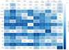 |
Fig. 22 Pearson correlation coefficients of the relations between molecular abundances and molecular hydrogen density, considering the total sample (first column), the molecular cloud of the points (second, third, and fourth columns), the extinction bins (fifth, sixth, and seventh columns) and the density bins (eighth, ninth, and tenth columns). Numbers in brackets correspond to the null hypothesis probability in each case, i.e. probability of no relation between variables, where a value higher than 0.001 is considered to indicate no relation at all. |
8 Comparison between Taurus, Perseus, and Orion
The C18O column density is widely used as a tracer of the gas mass in our galaxy and other galaxies. The reliability of this tracer is based on presenting a relatively uniform fractional abundance in interstellar molecular clouds. Based on our data, we estimated the mean C18O abundances in Taurus, Perseus, and Orion. The obtained values are: X(C18O) = (1.4 ± 0.7) × 10−7 for Taurus, X(C18O) = (2.1 ± 1.8) × 10−7 for Perseus, and X(C18O) = (1.6 ± 1.0) × 10−7 for Orion. These values are in good agreement with those obtained by previous works, as Frerking et al. (1989) in Taurus, Treviño-Morales et al. (2019) in Monoceros R2, and Roueff et al. (2021) in Orion B. Therefore, our results corroborate the idea that the abundance of C18O is quite stable at scales of molecular clouds, and is therefore a good gas mass tracer for large-scale surveys and extragalactic research.
We derived the mean values of the 13CO/C18O abundance ratio for the three star-forming regions, obtaining values of 13CO/C18O = 10.9 ± 7.5 for Taurus, 13CO/C18O = 17.3 ± 11.5 for Perseus, and 13CO/C18O = 23.7 ± 10.4 for Orion. The expected value is 13CO/C18O = 7.5−9.8, assuming 12C/13C = 57−67 and 16O/18O = 500−600 (Gerin et al. 2015; Langer & Penzias 1990; Wilson & Rood 1994). As mentioned in Sect. 5.7, the 13CO/C18O abundance ratio increases in regions of enhanced UV field (Shimajiri et al. 2014; Ishii et al. 2019; Areal et al. 2018). This variation is interpreted in terms of the selective photodissociation and isotopic fractionation (see Bron et al. 2018; Fuente et al. 2019). This effect is produced because the more abundant CO isotopolog shields itself from the effect of UV photons more efficiently than less abundant isotopologs (Stark et al. 2014; Visser et al. 2009). Our data confirm this trend in Orion, although the observed positions are located at a distance >1 pc from the ionized nebula M 42, which shows that the whole cloud is illuminated by a strong UV field emitted by young massive stars in the Trapezium cluster (Pabst et al. 2019). In contrast to X(C18O), which presents uniform abundance in the three regions, the mean 13CO abundance is a factor of approximately two higher in Orion than in Taurus. One interesting question pertains to whether the observed variation in the 13CO abundance is related to a variation in the 12CO/13CO ratio (Roueff et al. 2015; Colzi et al. 2020) or is revealing variations for a higher 12CO abundance in Orion. Because of the higher gas temperature and incident UV field in Orion, selective photodissociation would work in the direction of increasing N(12CO)/N(13CO) in Orion with respect to Taurus. Therefore, a higher 12CO abundance in Orion stands as the most likely explanation. Our results are based on significant approximations (one single phase, gas-dust thermalization), and therefore a detailed multi-transition study of these compounds is required to confirm this result.
Apart from 13CO, C18O, and H2S, the abundances of all the studied species decrease following the sequence Taurus, Perseus, and Orion. This might be interpreted considering the observed relations between the molecular abundances and the molecular hydrogen density, and the different density distributions of the positions observed in Taurus, Perseus, and Orion (see Fig. 8). It should be noted that the relation between CS abundance and density does not present significant differences between molecular clouds. However, the abundances of the protonated compounds HCO+ (and isotopologs) and HCS+ are systematically lower in Orion than in Taurus and Perseus for similar values of the molecular hydrogen density and visual extinction. To a lesser extent, this behavior is also observed in H13CN. A detailed modeling of the chemistry including all the species is required to discern the cause of this difference.
9 The extragalactic connection
Our data provide a comprehensive view of the abundance behavior of the most commonly observed species in molecular clouds, and it is interesting to compare them with extragalactic chemical studies. In most cases, the spatial resolution of current telescopes does not allow molecular clouds in external galaxies to be resolved, and therefore millimeter observations are used to measure cloud-weighted molecular abundances. To compare with external galaxies we computed mean values of observed molecular column densities and abundances in Taurus, Perseus, and Orion (Table 4). We caution that these mean values were computed using only detections. The majority of the detections correspond to dense gas (n(H2) > 104 cm−3) located in regions with AV > 8 mag and therefore the obtained abundances are representative of the dense phase. We would also like to reiterate the selection criteria applied for the positions of the GEMS program. The positions were selected to avoid protostars and shocks. Nevertheless, there are differences between the abundances measured in Taurus, Perseus, and Orion. The greatest differences between these averaged values are found for the N(13CO)/N(C18O) ( ) and the N(HCO+)/N(H13CO+) (
 ) ratios. Both
  and
and  increase with star formation activity following the sequence Taurus, Perseus, and Orion. This progressive increase is related to the different density distribution, average gas and dust temperatures, and incident UV field.
In Table 4, we compare the mean column densities in Taurus, Perseus, and Orion with those observed in a sample of galaxies including the starburst galaxies M 83, M 82, and NGC 253, the galaxies hosting an active galactic nucleus (AGN) M 51, NGC 1068, and NGC 7469, and the ultra-luminous infrared galaxies (ULIRGs) Arp 220 and Mrk 231. Aladro et al. (2015) carried out a molecular survey of this sample at λ = 3 mm using the IRAM 30 m telescope, producing a uniform database that can be easily compared with our observations. Moreover, the molecular abundances were derived using the same rotational lines as in this work. Aladro et al. (2015) did not detect H13CO+ towards NGC 1068. We used the data reported by Usero et al. (2004) to estimate N(HCO+) and N(H13CO+) by assuming the same source size and using the same methodology as Aladro et al. (2015) (LTE and Trot = 10 K). The obtained values are shown in Table 4.
The values of  are lower in the sample of galaxies considered than in GEMS sample. Moreover, we do not observe any increase with star formation activity. Instead, N(13CO)/N(C18O) ~ 3−6 in starburstsand AGNs, and decreases to ~1 in ULIRGs.This suggests that at scales of the whole galaxy,
  is not determined by the star formation activity but by optical depth effects and variations in the carbon and oxygen isotopic ratio because of stellar nucleosynthesis (Henkel et al. 1993, 1998; Wang et al. 2004). Jiménez-Donaire et al. (2017) carried out a survey of 13CO and C18O in a sample of nine nearby spiral galaxies. These latter authors found an average value of
  = 7.9 ± 0.8 measured in the whole galaxy and
  = 6.0 ± 0.9 for the central regions of the galaxies, that is,
  seems to be anti-correlated with star formation activity. These same authors, using higher spatial resolution ALMA observations (beam ~ 8″ < 400 pc) of NGC 3351, NGC 3627, and NGC 4321, observed that when zooming into the central regions,
  increases in a narrow ring at R ~500 pc. As the authors discussed, this increase in
  might be related to the enhanced star formation in these regions, which are fed by gas flows along the bars. Thus, the
  could be a diagnostic of star formation at scales comparable to the size of a giant molecular cloud, namely approximately a few hundred parsecs, but fails at scales of the whole galaxy. Moreover, accurate determination of the local 12C/13C and 16O/18O isotopic ratios is required for the correct comparison with galactic patterns and chemical models.
In the GEMS sample, the N(HCO+)/N(H13CO+) ratio is correlated with local star formation activity. Despite the limitations of our comparison, we observe the same trend in the galaxies sample. In M 83,  is similar to those measured in Taurus and Perseus, suggesting that the J = 1 →0 emission of these species is dominated by low- and intermediate-mass star forming regions. On the contrary, the other galaxies present
  > 10, suggesting that the emission could be dominated by massive star forming regions. In Taurus, the low estimated value of the N(HCO+)/N(H13CO+) ratio is not a chemical effect, but the consequence of a thick absorbing envelope that leads to a systematic underestimation of the HCO+ abundance when using one-phase models and the optically thick J = 1 →0 line. This thick envelope seems to be absent in Orion more likely because of the enhanced UV field that photodissociates the molecules at low visual extinctions. The similarity between the N(HCO+)/N(H13CO+) in Orion and those in starburst might be the consequence of the cloud properties in these regions where the ambient UV field is expected to be higher than in our galaxy (see, e.g., Fuente et al. 2005, 2006, 2008). The same trend is observed in N(HCN/N(H13CN).
It is interesting to discuss the N(H13CO+)/N(H13CN) (or N(HCO+))/N(HCN)) ratio, which is commonly used to differentiate between starburst- and AGN-dominated chemistry (see, e.g., García-Burillo et al. 2008). Indeed, the abundance of H13CO+ is highest in the M 82 galaxy which is considered as the prototype of evolved starburst with a photon-dominated chemistry in the nuclear region (Fuente et al. 2005, 2006, 2008). In contrast, H13CN is especially abundant in the active galaxy NGC 1068 and the ULIRGS Arp 220 and Mrk 231. The extraordinary abundance of HCN in these galaxies have been widely discussed by several authors that proposed mechanical heating, shocks, and X-rays as physical agents to boost the abundance of HCN (Usero et al. 2004; García-Burillo et al. 2008, 2014; Pérez-Beaupuits et al. 2009; Viti et al. 2014). We do not see a clear variation of the N(H13CO+)/N(H13CN) in the GEMS sample. We recall that GEMS positions were selected to avoid protostars, HII regions, and bipolar outflows. The difference between the N(H13CO+)/N(H13CN) ratios in GEMS clouds and those towards AGNs and ULIRGS supports the interpretation that the emission of H13CN in these galaxies is dominated by the gas associated with XDRs and shocks.
Viti (2017) analyzed grids of time-dependent chemical models, varying in gas density, temperature, cosmic ray ionization rate, and radiation field to calculate abundances and line intensities in order to compare with molecular observations in external galaxies. This latter study found that line intensities and line ratios from different chemical models can be very similar, leading to a large degeneracy. This degeneracy can be partially removed if chemical abundances and abundance ratios are used instead for the comparison. We provide tables of chemical abundances for three Galactic prototypical star forming regions that could be useful to interpret molecular data in external galaxies even if our data are not representative of the whole molecular cloud.
Mean column densities obtained in this work for Taurus, Perseus, and Orion and column densities observed in a sample of nearby galaxies.
10 Summary and conclusions
We present the molecular database of the GEMS project. This program is focused on the observation of starless cores in filaments of the nearby star-forming regions Taurus, Perseus, and Orion. These regions have different degrees of star formation activity, and therefore different physical conditions, providing a possibility to explore the effect of environment on gas chemistry. The project includes observations towards 305 positions distributed in 27 cuts that have been selected to avoid recently formed stars and their associated bipolar outflows. The gas chemistry in these positions is therefore not affected by the shocks produced by these energetic phenomena and/or the UV radiation coming from internal sources. Our project is characterizing the molecular cloud chemistry during the pre-stellar phase. The number of positions allows an unprecedented analysis of the statistical trends shown by the molecular abundances in a wide range of physical conditions.
We carried out a multi-transition analysis of the CS molecule and its isotopologs C34S and 13CS to derive the gas physical conditions, applying the MCMC methodology with a Bayesian inference approach, and using the RADEX code. We derived the molecular hydrogen abundance for 244 positions. Assuming the molecular hydrogen densities derived from the CS multi-transition fitting and using the RADEX code, we determined the molecular abundances for the following species: 13CO, C18O, HCO+, H13CO+, HC18O+, H13CN, HNC, HCS+, SO, 34SO, H2S, and OCS. We estimated the o-H2S abundances using the specific collisional rates recently calculated by Dagdigian (2020). We analyzed the relation between the molecular abundances and the gas physical parameters (kinetic temperature, extinction, and molecular hydrogen density), exploring the degree of correlation between parameters by the computation of the Pearson, Spearman, and Kendall correlation coefficients. Our main results are as follows:
-
Taurus shows the lowest mean density, with a peaky distribution at n(H2) ~ 2 × 104 cm−3 Higher density values, and wider density distributions are found in Perseus and Orion, with mean values of n(H2) ~ 4 × 104 cm−3 and ~6 × 104 cm−3, respectively. The wider density distribution in Perseus and Orion is the consequence of the superposition of regions with different environmental conditions resulting from the feedback of recently formed stars.
-
Relations between molecules themselves reveal strong linear correlations that define three families of species: (i) the CO isotopologs 13CO, C18O; (ii) H13CO+, HC18O+, H13CN, and HNC; and (iii) the S-bearing molecules CS, SO, 34SO, H2S, and OCS.
-
Only 13CO and C18O show a correlation with gas kinetic temperature. In the shielded gas, we observe an increasing relation between the abundances of these species with the gas kinetic temperature, until TK ~ 15 K. Beyond this value, the abundance remains constant with a large scatter. The X(13CO)/X(C18O) increases in the cloud border as the consequence of selective photodissociation and isotopic fractionation.
-
The abundances of H13CO+, HC18O+, H13CN, and HNC are well correlated and all of them decrease with molecular hydrogen density, which seems to be one of the main factors determining their abundances in starless cores. This anti-correlation spans over around three orders of magnitude in density, from n(H2) ~ 103 cm−3 to n(H2) ~ 106 cm−3.
-
Strong linear correlations are also found between abundances of the S-bearing species CS, SO, 34SO, H2S, and OCS, which is very likely caused by the decrease of sulfur in gas phase. Under the reasonable assumption that the S/H in gas phase, (S/H)gas, is correlated with the abundances of these species, we obtain that (S/H)gas ∝ n−0.6 in the n(H2) ~ 103−106 cm−3 density range.
-
The observed anti-correlation of the studied molecular abundances with density is always stronger in the case of the Taurus cloud. Perseus and Orion show weaker anti-correlations with H2 density with smaller correlation parameters. However, we do recover strong anti-correlations with density for bins of 8−20 mag in Perseus and >20 mag in Orion. This shows that the dark region is located at a different visual extinction depending on the star formation activity.
In addition to the statistical analysis, we computed mean values of molecular column densities and abundances in Taurus, Perseus, and Orion in order to compare with extragalactic studies. The C18O abundance is quite uniform in the three clouds, suggesting that its column density is a good gas mass tracer. However, the abundance of most species decreases, following the sequence Taurus, Perseus, and Orion, as a consequence of density distributions in these clouds.
The GEMS project provides an unprecedented database with which to investigate the gas chemistry in molecular clouds and starless cores. This database is also useful to compare with molecular observations in external galaxies. A complete analysis of the chemical processes involved in the detected relations requires the comparison of observational data with predictions of chemical models, which will be carried out in a forthcoming paper.
Acknowledgements
We thank the Spanish the Spanish Ministerio de Ciencia e Innovación for funding support through AYA2016-75066-C2-1/2-P and PID2019-106235GB-I00. S.G.-B. acknowledges support through grants PGC2018-094671-B-I00 (MICIU/AEI/FEDER,UE) and PID2019-106027GA-C44. J.R.G. acknowledges support through grants AYA2017-85111-P and PID2019-106110GB-I00. I.J.-S. has received partial support from the Spanish FEDER (project number ESP2017-86582-C4-1-R) and the State Research Agency (AEI; project number PID2019-105552RB-C41). SPTM acknowledges to the European Union’s Horizon 2020 research and innovation program for funding support given under grant agreement No 639459 (PROMISE). We thank the anonymous referee for valuable comments that improved the manuscript.
References
- Agúndez, M., & Wakelam, V. 2013, Chem. Rev., 113, 8710 [Google Scholar]
- Agúndez, M., Marcelino, N., Cernicharo, J., Roueff, E., & Tafalla, M. 2019, A&A, 625, A147 [NASA ADS] [CrossRef] [EDP Sciences] [Google Scholar]
- Aladro, R., Martín, S., Riquelme, D., et al. 2015, A&A, 579, A101 [NASA ADS] [CrossRef] [EDP Sciences] [Google Scholar]
- Anantharamaiah, K. R., Viallefond, F., Mohan, N. R., Goss, W. M., & Zhao, J. H. 2000, ApJ, 537, 613 [Google Scholar]
- Anderl, S., Maret, S., Cabrit, S., et al. 2016, A&A, 591, A3 [NASA ADS] [CrossRef] [EDP Sciences] [Google Scholar]
- Anderson, D. E., Bergin, E. A., Maret, S., & Wakelam, V. 2013, ApJ, 779, 141 [Google Scholar]
- André, P., Men’shchikov, A., Bontemps, S., et al. 2010, A&A, 518, L102 [NASA ADS] [CrossRef] [EDP Sciences] [Google Scholar]
- Anglada, G., Estalella, R., Pastor, J., Rodriguez, L. F., & Haschick, A. D. 1996, ApJ, 463, 205 [Google Scholar]
- Areal, M. B., Paron, S., Celis Peña, M., & Ortega, M. E. 2018, A&A, 612, A117 [NASA ADS] [CrossRef] [EDP Sciences] [Google Scholar]
- Asplund, M., Grevesse, N., Sauval, A. J., & Scott, P. 2009, ARA&A, 47, 481 [NASA ADS] [CrossRef] [Google Scholar]
- Baan, W. A., Henkel, C., Loenen, A. F., Baudry, A., & Wiklind, T. 2008, A&A, 477, 747 [NASA ADS] [CrossRef] [EDP Sciences] [Google Scholar]
- Bachiller, R., & Cernicharo, J. 1984, A&A, 140, 414 [NASA ADS] [Google Scholar]
- Bachiller, R., & Pérez Gutiérrez, M. 1997, ApJ, 487, L93 [Google Scholar]
- Bally, J. 2008, Overview of the Orion Complex, ed. B. Reipurth (USA: Astronomical Society of the Pacific), 4, 459 [NASA ADS] [Google Scholar]
- Bally, J., Langer, W. D., Stark, A. A., & Wilson, R. W. 1987, ApJ, 312, L45 [NASA ADS] [CrossRef] [Google Scholar]
- Bayet, E., Aladro, R., Martín, S., Viti, S., & Martín-Pintado, J. 2009, ApJ, 707, 126 [Google Scholar]
- Benson, P. J., & Myers, P. C. 1989, ApJS, 71, 89 [Google Scholar]
- Bernard, J.-P., Paradis, D., Marshall, D. J., et al. 2010, A&A, 518, L88 [NASA ADS] [CrossRef] [EDP Sciences] [Google Scholar]
- Bohlin, R. C., Savage, B. D., & Drake, J. F. 1978, ApJ, 224, 132 [NASA ADS] [CrossRef] [Google Scholar]
- Boogert, A. C. A., Schutte, W. A., Helmich, F. P., Tielens, A. G. G. M., & Wooden, D. H. 1997, A&A, 317, 929 [NASA ADS] [Google Scholar]
- Bracco, A., Palmeirim, P., André, P., et al. 2017, A&A, 604, A52 [NASA ADS] [CrossRef] [EDP Sciences] [Google Scholar]
- Bron, E., Daudon, C., Pety, J., et al. 2018, A&A, 610, A12 [NASA ADS] [CrossRef] [EDP Sciences] [Google Scholar]
- Bronfman, L., Nyman, L. A., & May, J. 1996, A&AS, 115, 81 [Google Scholar]
- Brown, A. G. A., Hartmann, D., & Burton, W. B. 1995, A&A, 300, 903 [NASA ADS] [Google Scholar]
- Bulut, N., Roncero, O., Aguado, A., et al. 2021, A&A, 646, A5 [NASA ADS] [CrossRef] [EDP Sciences] [Google Scholar]
- Calmonte, U., Altwegg, K., Balsiger, H., et al. 2016, MNRAS, 462, S253 [CrossRef] [Google Scholar]
- Cambrésy, L. 1999, A&A, 345, 965 [NASA ADS] [Google Scholar]
- Caselli, P., Walmsley, C. M., Terzieva, R., & Herbst, E. 1998, ApJ, 499, 234 [Google Scholar]
- Caselli, P., Walmsley, C. M., Zucconi, A., et al. 2002, ApJ, 565, 344 [Google Scholar]
- Cazaux, S., Martín-Doménech, R., Chen, Y. J., Muñoz Caro, G. M., & González Díaz C. 2017, ApJ, 849, 80 [Google Scholar]
- Cernicharo, J., & Guelin, M. 1987, A&A, 176, 299 [NASA ADS] [Google Scholar]
- Colzi, L., Fontani, F., Caselli, P., et al. 2018, A&A, 609, A129 [NASA ADS] [CrossRef] [EDP Sciences] [Google Scholar]
- Colzi, L., Sipilä, O., Roueff, E., Caselli, P., & Fontani, F. 2020, A&A, 640, A51 [CrossRef] [EDP Sciences] [Google Scholar]
- Crockett, N. R., Bergin, E. A., Neill, J. L., et al. 2014, ApJ, 781, 114 [NASA ADS] [CrossRef] [Google Scholar]
- Curtis, E. I., & Richer, J. S. 2011, MNRAS, 410, 75 [Google Scholar]
- Da Rio, N., Robberto, M., Hillenbrand, L. A., Henning, T., & Stassun, K. G. 2012, ApJ, 748, 14 [Google Scholar]
- Dagdigian, P. J. 2020, MNRAS, 494, 5239 [NASA ADS] [CrossRef] [Google Scholar]
- Daniel, F., Gérin, M., Roueff, E., et al. 2013, A&A, 560, A3 [NASA ADS] [CrossRef] [EDP Sciences] [Google Scholar]
- Davis, C. J., Chrysostomou, A., Hatchell, J., et al. 2010, MNRAS, 405, 759 [NASA ADS] [Google Scholar]
- Denis-Alpizar, O., Stoecklin, T., Halvick, P., & Dubernet, M.-L. 2013, J. Chem. Phys., 139, 204304 [NASA ADS] [CrossRef] [Google Scholar]
- Denis-Alpizar, O., Stoecklin, T., Guilloteau, S., & Dutrey, A. 2018, MNRAS, 478, 1811 [Google Scholar]
- Draine, B. T. 1978, ApJS, 36, 595 [NASA ADS] [CrossRef] [Google Scholar]
- Dubernet, M. L., Daniel, F., Grosjean, A., & Lin, C. Y. 2009, A&A, 497, 911 [NASA ADS] [CrossRef] [EDP Sciences] [Google Scholar]
- Dumouchel, F., Kłos, J., & Lique, F. 2011, Phys. Chem. Chem. Phys., 13, 8204 [NASA ADS] [CrossRef] [Google Scholar]
- Dutrey, A., Guilloteau, S., & Guelin, M. 1997, A&A, 317, L55 [NASA ADS] [Google Scholar]
- Dutrey, A., Wakelam, V., Boehler, Y., et al. 2011, A&A, 535, A104 [NASA ADS] [CrossRef] [EDP Sciences] [Google Scholar]
- Enoch, M. L., Young, K. E., Glenn, J., et al. 2006, ApJ, 638, 293 [Google Scholar]
- Esplugues, G. B., Viti, S., Goicoechea, J. R., & Cernicharo, J. 2014, A&A, 567, A95 [NASA ADS] [CrossRef] [EDP Sciences] [Google Scholar]
- Esquej, P., Alonso-Herrero, A., González-Martín, O., et al. 2014, ApJ, 780, 86 [Google Scholar]
- Fehér, O., Tóth, L. V., Ward-Thompson, D., et al. 2016, A&A, 590, A75 [NASA ADS] [CrossRef] [EDP Sciences] [Google Scholar]
- Flower, D. R. 1999, MNRAS, 305, 651 [Google Scholar]
- Foreman-Mackey, D., Hogg, D. W., Lang, D., & Goodman, J. 2013, PASP, 125, 306 [Google Scholar]
- Frau, P., Girart, J. M., & Beltrán, M. T. 2012, A&A, 537, L9 [NASA ADS] [CrossRef] [EDP Sciences] [Google Scholar]
- Frerking, M. A., Keene, J., Blake, G. A., & Phillips, T. G. 1989, ApJ, 344, 311 [Google Scholar]
- Friesen, R. K., Pineda, J. E., co-PIs, et al. 2017, ApJ, 843, 63 [NASA ADS] [CrossRef] [Google Scholar]
- Fuente, A., García-Burillo, S., Gerin, M., et al. 2005, ApJ, 619, L155 [Google Scholar]
- Fuente, A., García-Burillo, S., Gerin, M., et al. 2006, ApJ, 641, L105 [Google Scholar]
- Fuente, A., García-Burillo, S., Usero, A., et al. 2008, A&A, 492, 675 [NASA ADS] [CrossRef] [EDP Sciences] [Google Scholar]
- Fuente, A., Cernicharo, J., Agúndez, M., et al. 2010, A&A, 524, A19 [NASA ADS] [CrossRef] [EDP Sciences] [Google Scholar]
- Fuente, A., Caselli, P., McCoey, C., et al. 2012, A&A, 540, A75 [NASA ADS] [CrossRef] [EDP Sciences] [Google Scholar]
- Fuente, A., Cernicharo, J., Roueff, E., et al. 2016, A&A, 593, A94 [NASA ADS] [CrossRef] [EDP Sciences] [Google Scholar]
- Fuente, A., Goicoechea, J. R., Pety, J., et al. 2017, ApJ, 851, L49 [NASA ADS] [CrossRef] [Google Scholar]
- Fuente, A., Navarro, D. G., Caselli, P., et al. 2019, A&A, 624, A105 [NASA ADS] [CrossRef] [EDP Sciences] [Google Scholar]
- García-Burillo, S., Graciá-Carpio, J., Usero, A., et al. 2008, EAS Pub. Ser., 31, 85 [Google Scholar]
- García-Burillo, S., Combes, F., Usero, A., et al. 2014, A&A, 567, A125 [NASA ADS] [CrossRef] [EDP Sciences] [Google Scholar]
- Gatley, I., Becklin, E. E., Mattews, K., et al. 1974, ApJ, 191, L121 [Google Scholar]
- Geballe, T. R., Baas, F., Greenberg, J. M., & Schutte, W. 1985, A&A, 146, L6 [NASA ADS] [Google Scholar]
- Genzel, R., Weitzel, L., Tacconi-Garman, L. E., et al. 1995, ApJ, 444, 129 [Google Scholar]
- Gerin, M., Ruaud, M., Goicoechea, J. R., et al. 2015, A&A, 573, A30 [NASA ADS] [CrossRef] [EDP Sciences] [Google Scholar]
- Getman, K. V., Feigelson, E. D., Kuhn, M. A., & Garmire, G. P. 2019, MNRAS, 487, 2977 [Google Scholar]
- Goicoechea, J. R., & Le Bourlot, J. 2007, A&A, 467, 1 [NASA ADS] [CrossRef] [EDP Sciences] [Google Scholar]
- Goicoechea, J. R., Pety, J., Gerin, M., et al. 2006, A&A, 456, 5655 [NASA ADS] [CrossRef] [EDP Sciences] [Google Scholar]
- Goicoechea, J. R., Compiègne, M., & Habart, E. 2009a, ApJ, 699, L165 [Google Scholar]
- Goicoechea, J. R., Pety, J., Gerin, M., Hily-Blant, P., & Le Bourlot, J. 2009b, A&A, 498, 771 [NASA ADS] [CrossRef] [EDP Sciences] [Google Scholar]
- Goicoechea, J. R., Pety, J., Cuadrado, S., et al. 2016, Nature, 537, 207 [NASA ADS] [CrossRef] [Google Scholar]
- Goicoechea, J. R., Santa-Maria, M. G., Bron, E., et al. 2019, A&A, 622, A91 [NASA ADS] [CrossRef] [EDP Sciences] [Google Scholar]
- Goldsmith, P. F., Langer, W. D., Ellder, J., Kollberg, E., & Irvine, W. 1981, ApJ, 249, 524 [Google Scholar]
- Goldsmith, P. F., Irvine, W. M., Hjalmarson, A., & Ellder, J. 1986, ApJ, 310, 383 [NASA ADS] [CrossRef] [PubMed] [Google Scholar]
- Goldsmith, P. F., Heyer, M., Narayanan, G., et al. 2008, ApJ, 680, 428 [NASA ADS] [CrossRef] [Google Scholar]
- Gonzalez Garcia, M., Le Bourlot, J., Le Petit, F., & Roueff, E. 2008, A&A, 485, 127 [NASA ADS] [CrossRef] [EDP Sciences] [Google Scholar]
- Goodman, J., & Weare, J. 2010, Commun. Appl. Math. Comput. Sci., 5, 65 [Google Scholar]
- Gratier, P., Majumdar, L., Ohishi, M., et al. 2016, ApJS, 225, 25 [Google Scholar]
- Green, S., & Chapman, S. 1978, ApJS, 37, 169 [Google Scholar]
- Griffin, M. J., Abergel, A., Abreu, A., et al. 2010, A&A, 518, L3 [EDP Sciences] [Google Scholar]
- Guelin, M., Langer, W. D., & Wilson, R. W. 1982, A&A, 107, 107 [NASA ADS] [Google Scholar]
- Guilloteau, S., Reboussin, L., Dutrey, A., et al. 2016, A&A, 592, A124 [NASA ADS] [CrossRef] [EDP Sciences] [Google Scholar]
- Guzmán, V., Pety, J., Goicoechea, J. R., Gerin, M., & Roueff, E. 2011, A&A, 534, A49 [NASA ADS] [CrossRef] [EDP Sciences] [Google Scholar]
- Guzmán, V., Pety, J., Gratier, P., et al. 2012a, A&A, 543, L1 [NASA ADS] [CrossRef] [EDP Sciences] [Google Scholar]
- Guzmán, V., Roueff, E., Gauss, J., et al. 2012b, A&A, 548, A94 [NASA ADS] [CrossRef] [EDP Sciences] [Google Scholar]
- Guzmán, V. V., Goicoechea, J. R., Pety, J., et al. 2013, A&A, 560, A73 [NASA ADS] [CrossRef] [EDP Sciences] [Google Scholar]
- Hacar, A., Tafalla, M., Kauffmann, J., & Kovács, A. 2013, A&A, 554, A55 [NASA ADS] [CrossRef] [EDP Sciences] [Google Scholar]
- Hacar, A., Alves, J., Tafalla, M., & Goicoechea, J. R. 2017a, A&A, 602, L2 [NASA ADS] [CrossRef] [EDP Sciences] [Google Scholar]
- Hacar, A., Tafalla, M., & Alves, J. 2017b, A&A, 606, A123 [NASA ADS] [CrossRef] [EDP Sciences] [Google Scholar]
- Hacar, A., Tafalla, M., Forbrich, J., et al. 2018, A&A, 610, A77 [NASA ADS] [CrossRef] [EDP Sciences] [Google Scholar]
- Hacar, A., Bosman, A. D., & van Dishoeck, E. F. 2020, A&A, 635, A4 [CrossRef] [EDP Sciences] [Google Scholar]
- Hatchell, J., Richer, J. S., Fuller, G. A., et al. 2005, A&A, 440, 151 [NASA ADS] [CrossRef] [EDP Sciences] [Google Scholar]
- Hatchell, J., Fuller, G. A., & Richer, J. S. 2007a, A&A, 472, 187 [NASA ADS] [CrossRef] [EDP Sciences] [Google Scholar]
- Hatchell, J., Fuller, G. A., Richer, J. S., Harries, T. J., & Ladd, E. F. 2007b, A&A, 468, 1009 [NASA ADS] [CrossRef] [EDP Sciences] [Google Scholar]
- Heithausen, A., Böttner, C., & Walter, F. 2008, A&A, 488, 597 [NASA ADS] [CrossRef] [EDP Sciences] [Google Scholar]
- Henkel, C., Mauersberger, R., Wiklind, T., et al. 1993, A&A, 268, L17 [Google Scholar]
- Henkel, C., Chin, Y. N., Mauersberger, R., & Whiteoak, J. B. 1998, A&A, 329, 443 [Google Scholar]
- Hernández Vera, M., Lique, F., Dumouchel, F., Hily-Blant, P., & Faure, A. 2017, MNRAS, 468, 1084 [NASA ADS] [CrossRef] [Google Scholar]
- Hillenbrand, L. A. 1997, AJ, 113, 1733 [NASA ADS] [CrossRef] [Google Scholar]
- Hily-Blant, P., Walmsley, M., Pineau Des Forêts, G., & Flower, D. 2010, A&A, 513, A41 [NASA ADS] [CrossRef] [EDP Sciences] [Google Scholar]
- Hirota, T., & Yamamoto, S. 2006, ApJ, 646, 258 [Google Scholar]
- Hirota, T., Yamamoto, S., Mikami, H., & Ohishi, M. 1998, ApJ, 503, 717 [NASA ADS] [CrossRef] [Google Scholar]
- Ishii, S., Nakamura, F., Shimajiri, Y., et al. 2019, PASJ, 71, S9 [Google Scholar]
- James, T. A., Viti, S., Holdship, J., & Jiménez-Serra, I. 2020, A&A, 634, A17 [EDP Sciences] [Google Scholar]
- Jiménez-Donaire, M. J., Cormier, D., Bigiel, F., et al. 2017, ApJ, 836, L29 [Google Scholar]
- Jiménez-Escobar, A., & Muñoz Caro, G. M. 2011, A&A, 536, A91 [NASA ADS] [CrossRef] [EDP Sciences] [Google Scholar]
- Jiménez-Escobar, A., Muñoz Caro, G. M., Ciaravella, A., et al. 2012, ApJ, 751, L40 [Google Scholar]
- Jiménez-Escobar, A., Muñoz Caro, G. M., & Chen, Y. J. 2014, MNRAS, 443, 343 [Google Scholar]
- Jiménez-Serra, I., Caselli, P., Martín-Pintado, J., & Hartquist, T. W. 2008, A&A, 482, 549 [NASA ADS] [CrossRef] [EDP Sciences] [Google Scholar]
- Johnstone, D.,& Bally, J. 1999, ApJ, 510, L49 [Google Scholar]
- Johnstone, D.,& Bally, J. 2006, ApJ, 653, 383 [Google Scholar]
- Kainulainen, J., Stutz, A. M., Stanke, T., et al. 2017, A&A, 600, A141 [NASA ADS] [CrossRef] [EDP Sciences] [Google Scholar]
- Karnath, N., Megeath, S. T., Tobin, J. J., et al. 2020, ApJ, 890, 129 [Google Scholar]
- Kim, S., Lee, C. W., Gopinathan, M., et al. 2020, ApJ, 891, 169 [Google Scholar]
- Kirk, H., Johnstone, D., & Di Francesco, J. 2006, ApJ, 646, 1009 [Google Scholar]
- Kirk, J. M., Ward-Thompson, D., Palmeirim, P., et al. 2013, MNRAS, 432, 1424 [NASA ADS] [CrossRef] [Google Scholar]
- Kirk, H., Friesen, R. K., Pineda, J. E., et al. 2017, ApJ, 846, 144 [Google Scholar]
- Kong, S., Arce, H. G., Sargent, A. I., et al. 2019, ApJ, 882, 45 [NASA ADS] [CrossRef] [Google Scholar]
- Kounkel, M., Hartmann, L., Loinard, L., et al. 2017, ApJ, 834, 142 [Google Scholar]
- Kutner, M. L., Evans, N. J., I., & Tucker, K. D. 1976, ApJ, 209, 452 [Google Scholar]
- Laas, J. C., & Caselli, P. 2019, A&A, 624, A108 [CrossRef] [EDP Sciences] [Google Scholar]
- Lada, C. J., Alves, J., & Lada, E. A. 1996, AJ, 111, 1964 [Google Scholar]
- Lada, C. J., Muench, A. A., Haisch, Karl E., J., et al. 2000, AJ, 120, 3162 [Google Scholar]
- Lada, C. J., Lombardi, M., & Alves, J. F. 2010, ApJ, 724, 687 [NASA ADS] [CrossRef] [Google Scholar]
- Langer, W. D., & Penzias, A. A. 1990, ApJ, 357, 477 [Google Scholar]
- Launhardt, R., Evans, Neal J., I., Wang, Y., et al. 1998, ApJS, 119, 59 [Google Scholar]
- Le Bourlot, J., Le Petit, F., Pinto, C., Roueff, E., & Roy, F. 2012, A&A, 541, A76 [NASA ADS] [CrossRef] [EDP Sciences] [Google Scholar]
- Le Gal, R., Hily-Blant, P., Faure, A., et al. 2014, A&A, 562, A83 [NASA ADS] [CrossRef] [EDP Sciences] [Google Scholar]
- Le Gal, R., Herbst, E., Dufour, G., et al. 2017, A&A, 605, A88 [NASA ADS] [CrossRef] [EDP Sciences] [Google Scholar]
- Le Gal, R., Öberg, K. I., Loomis, R. A., Pegues, J., & Bergner, J. B. 2019, ApJ, 876, 72 [Google Scholar]
- Le Gal, R., Öberg, K. I., Huang, J., et al. 2020, ApJ, 898, 131 [Google Scholar]
- Le Petit, F., Nehmé, C., Le Bourlot, J., & Roueff, E. 2006, ApJS, 164, 506 [NASA ADS] [CrossRef] [EDP Sciences] [Google Scholar]
- Linke, R. A., & Goldsmith, P. F. 1980, ApJ, 235, 437 [Google Scholar]
- Lique, F., & Spielfiedel, A. 2007, A&A, 462, 1179 [NASA ADS] [CrossRef] [EDP Sciences] [Google Scholar]
- Liszt, H. S., & Gerin, M. 2016, A&A, 585, A80 [Google Scholar]
- Liszt, H., & Lucas, R. 2001, A&A, 370, 576 [NASA ADS] [CrossRef] [EDP Sciences] [Google Scholar]
- Liszt, H. S., Wilson, R. W., Penzias, A. A., et al. 1974, ApJ, 190, 557 [Google Scholar]
- Liszt, H. S., Pety, J., & Lucas, R. 2010, A&A, 518, A45 [NASA ADS] [CrossRef] [EDP Sciences] [Google Scholar]
- Loison, J.-C., Wakelam, V., & Hickson, K. M. 2014, MNRAS, 443, 398 [Google Scholar]
- Loison, J.-C., Wakelam, V., Gratier, P., & Hickson, K. M. 2019a, MNRAS, 484, 2747 [Google Scholar]
- Loison, J.-C., Wakelam, V., Gratier, P., et al. 2019b, MNRAS, 485, 5777 [NASA ADS] [CrossRef] [Google Scholar]
- Loison, J.-C., Wakelam, V., Gratier, P., & Hickson, K. M. 2020, MNRAS, 498, 4663 [Google Scholar]
- Lombardi, M., Alves, J., & Lada, C. J. 2011, A&A, 535, A16 [NASA ADS] [CrossRef] [EDP Sciences] [Google Scholar]
- Lombardi, M., Bouy, H., Alves, J., & Lada, C. J. 2014, A&A, 568, C1 [Google Scholar]
- Lucas, R., & Liszt, H. S. 2002, A&A, 384, 1054 [NASA ADS] [CrossRef] [EDP Sciences] [Google Scholar]
- Luhman, K. L., Stauffer, J. R., Muench, A. A., et al. 2003, ApJ, 593, 1093 [Google Scholar]
- Luhman, K. L., Mamajek, E. E., Allen, P. R., & Cruz, K. L. 2009, ApJ, 703, 399 [Google Scholar]
- Maddalena, R. J., Morris, M., Moscowitz, J., & Thaddeus, P. 1986, ApJ, 303, 375 [NASA ADS] [CrossRef] [Google Scholar]
- Malinen, J., Juvela, M., Rawlings, M. G., et al. 2012, A&A, 544, A50 [NASA ADS] [CrossRef] [EDP Sciences] [Google Scholar]
- Marsh, K. A., Griffin, M. J., Palmeirim, P., et al. 2014, MNRAS, 439, 3683 [Google Scholar]
- Mathis, J. S., Rumpl, W., & Nordsieck, K. H. 1977, ApJ, 217, 425 [NASA ADS] [CrossRef] [Google Scholar]
- McKee, C. F. 1989, ApJ, 345, 782 [Google Scholar]
- Miotello, A., Facchini, S., van Dishoeck, E. F., et al. 2019, A&A, 631, A69 [NASA ADS] [CrossRef] [EDP Sciences] [Google Scholar]
- Mizuno, A., Onishi, T., Yonekura, Y., et al. 1995, ApJ, 445, L161 [Google Scholar]
- Monsch, K., Pineda, J. E., Liu, H. B., et al. 2018, ApJ, 861, 77 [Google Scholar]
- Muench, A. A., Lada, E. A., Lada, C. J., & Alves, J. 2002, ApJ, 573, 366 [NASA ADS] [CrossRef] [Google Scholar]
- Nakamura, F., Ishii, S., Dobashi, K., et al. 2019, PASJ, 71, S3 [Google Scholar]
- Narayanan, G., Heyer, M. H., Brunt, C., et al. 2008, ApJS, 177, 341 [Google Scholar]
- Navarro-Almaida, D., Le Gal, R., Fuente, A., et al. 2020, A&A 637, A39 [CrossRef] [EDP Sciences] [Google Scholar]
- Ochsendorf, B. B., Brown, A. G. A., Bally, J., & Tielens, A. G. G. M. 2015, ApJ, 808, 111 [NASA ADS] [CrossRef] [Google Scholar]
- Okada, Y., Pilleri, P., Berné, O., et al. 2013, A&A, 553, A2 [NASA ADS] [CrossRef] [EDP Sciences] [Google Scholar]
- Onishi, T., Mizuno, A., Kawamura, A., Ogawa, H., & Fukui, Y. 1996, ApJ, 465, 815 [Google Scholar]
- Onishi, T., Mizuno, A., Kawamura, A., Tachihara, K., & Fukui, Y. 2002, ApJ, 575, 950 [Google Scholar]
- Oppenheimer, M., & Dalgarno, A. 1974, ApJ, 192, 29 [Google Scholar]
- Ortiz-León, G. N., Loinard, L., Dzib, S. A., et al. 2018, ApJ, 865, 73 [Google Scholar]
- Pabst, C., Higgins, R., Goicoechea, J. R., et al. 2019, Nature, 565, 618 [NASA ADS] [CrossRef] [Google Scholar]
- Padoan, P., Cambrésy, L., & Langer, W. 2002, ApJ, 580, L57 [Google Scholar]
- Padovani, M., Hennebelle, P., & Galli, D. 2013, A&A, 560, A114 [NASA ADS] [CrossRef] [EDP Sciences] [Google Scholar]
- Padovani, M., Ivlev, A. V., Galli, D., et al. 2020, Space Sci. Rev., 216, 29 [Google Scholar]
- Palmeirim, P., André, P., Kirk, J., et al. 2013, A&A, 550, A38 [NASA ADS] [CrossRef] [EDP Sciences] [Google Scholar]
- Palumbo, M. E., Tielens, A. G. G. M., & Tokunaga, A. T. 1995, ApJ, 449, 674 [Google Scholar]
- Pérez-Beaupuits, J. P., Spaans, M., van der Tak, F. F. S., et al. 2009, A&A, 503, 459 [NASA ADS] [CrossRef] [EDP Sciences] [Google Scholar]
- Pety, J., Teyssier, D., Fossé, D., et al. 2005, A&A, 435, 885 [NASA ADS] [CrossRef] [EDP Sciences] [Google Scholar]
- Pety, J., Guzmán, V. V., Orkisz, J. H., et al. 2017, A&A, 599, A98 [NASA ADS] [CrossRef] [EDP Sciences] [Google Scholar]
- Phuong, N. T., Chapillon, E., Majumdar, L., et al. 2018, A&A, 616, L5 [NASA ADS] [CrossRef] [EDP Sciences] [Google Scholar]
- Pineda, J. E., Caselli, P., & Goodman, A. A. 2008, ApJ, 679, 481 [Google Scholar]
- Pineda, J. E., Goodman, A. A., Arce, H. G., et al. 2010, ApJ, 712, L116 [Google Scholar]
- Pineda, J. E., Offner, S. S. R., Parker, R. J., et al. 2015, Nature, 518, 213 [Google Scholar]
- Poglitsch, A., Waelkens, C., Geis, N., et al. 2010, A&A, 518, L2 [NASA ADS] [CrossRef] [EDP Sciences] [Google Scholar]
- Pon, A., Ochsendorf, B. B., Alves, J., et al. 2016, ApJ, 827, 42 [NASA ADS] [CrossRef] [Google Scholar]
- Punanova, A., Caselli, P., Pineda, J. E., et al. 2018, A&A, 617, A27 [NASA ADS] [CrossRef] [EDP Sciences] [Google Scholar]
- Rebull, L. M., Padgett, D. L., McCabe, C. E., et al. 2010, ApJS, 186, 259 [Google Scholar]
- Ridge, N. A., Di Francesco, J., Kirk, H., et al. 2006, AJ, 131, 2921 [Google Scholar]
- Rivière-Marichalar, P., Fuente, A., Goicoechea, J. R., et al. 2019, A&A, 628, A16 [NASA ADS] [CrossRef] [EDP Sciences] [Google Scholar]
- Robberto, M., Soderblom, D. R., Bergeron, E., et al. 2013, ApJS, 207, 10 [Google Scholar]
- Rolffs, R., Schilke, P., Wyrowski, F., et al. 2011, A&A, 529, A76 [NASA ADS] [CrossRef] [EDP Sciences] [Google Scholar]
- Roueff, E., Loison, J. C., & Hickson, K. M. 2015, A&A, 576, A99 [NASA ADS] [CrossRef] [EDP Sciences] [Google Scholar]
- Roueff, A., Gerin, M., Gratier, P., et al. 2021, A&A 645, A26 [Google Scholar]
- Ruffle, D. P., Hartquist, T. W., Caselli, P., & Williams, D. A. 1999, MNRAS, 306, 691 [Google Scholar]
- Sandell, G., & Knee, L. B. G. 2001, ApJ, 546, L49 [Google Scholar]
- Savage, C., Apponi, A. J., Ziurys, L. M., & Wyckoff, S. 2002, ApJ, 578, 211 [Google Scholar]
- Schilke, P., Walmsley, C. M., Pineau Des Forets, G., et al. 1992, A&A, 256, 595 [Google Scholar]
- Schmalzl, M., Kainulainen, J., Quanz, S. P., et al. 2010, ApJ, 725, 1327 [Google Scholar]
- Schnee, S., Caselli, P., Goodman, A., et al. 2007, ApJ, 671, 1839 [Google Scholar]
- Schnee, S., Enoch, M., Noriega-Crespo, A., et al. 2010, ApJ, 708, 127 [Google Scholar]
- Schöier, F. L., Jørgensen, J. K., van Dishoeck, E. F., & Blake, G. A. 2002, A&A, 390, 1001 [NASA ADS] [CrossRef] [EDP Sciences] [Google Scholar]
- Schuster, K. F., Kramer, C., Hitschfeld, M., Garcia-Burillo, S., & Mookerjea, B. 2007, A&A, 461, 143 [NASA ADS] [CrossRef] [EDP Sciences] [Google Scholar]
- Scourfield, M., Viti, S., García-Burillo, S., et al. 2020, MNRAS, 496, 5308 [Google Scholar]
- Semenov, D., Favre, C., Fedele, D., et al. 2018, A&A, 617, A28 [NASA ADS] [CrossRef] [EDP Sciences] [Google Scholar]
- Shimajiri, Y., Kitamura, Y., Saito, M., et al. 2014, A&A, 564, A68 [NASA ADS] [CrossRef] [EDP Sciences] [Google Scholar]
- Shimajiri, Y., André, P., Palmeirim, P., et al. 2019, A&A, 623, A16 [NASA ADS] [CrossRef] [EDP Sciences] [Google Scholar]
- Shingledecker, C. N., Lamberts, T., Laas, J. C., et al. 2020, ApJ, 888, 52 [CrossRef] [Google Scholar]
- Shirley, Y. L., Evans, Neal J., I., Young, K. E., Knez, C., & Jaffe, D. T. 2003, ApJS, 149, 375 [Google Scholar]
- Stark, G., Heays, A. N., Lyons, J. R., et al. 2014, ApJ, 788, 67 [Google Scholar]
- Steenbrugge, K. C., de Bruijne, J. H. J., Hoogerwerf, R., & de Zeeuw, P. T. 2003, A&A, 402, 587 [NASA ADS] [CrossRef] [EDP Sciences] [Google Scholar]
- Sternberg, A., & Dalgarno, A. 1995, ApJS, 99, 565 [NASA ADS] [CrossRef] [Google Scholar]
- Strickland, D. K., Heckman, T. M., Colbert, E. J. M., Hoopes, C. G., & Weaver, K. A. 2004, ApJS, 151, 193 [NASA ADS] [CrossRef] [Google Scholar]
- Suri, S., Sánchez-Monge, Á., Schilke, P., et al. 2019, A&A, 623, A142 [NASA ADS] [CrossRef] [EDP Sciences] [Google Scholar]
- Tafalla, M., & Santiago, J. 2004, A&A, 414, L53 [Google Scholar]
- Tafalla, M., & Hacar, A. 2015, A&A, 574, A104 [NASA ADS] [CrossRef] [EDP Sciences] [Google Scholar]
- Tafalla, M., Myers, P. C., Caselli, P., Walmsley, C. M., & Comito, C. 2002, ApJ, 569, 815 [Google Scholar]
- Tafalla, M., Myers, P. C., Caselli, P., & Walmsley, C. M. 2004, A&A, 416, 191 [NASA ADS] [CrossRef] [EDP Sciences] [Google Scholar]
- Tanabe, Y., Nakamura, F., Tsukagoshi, T., et al. 2019, PASJ, 71, S8 [Google Scholar]
- Tatematsu, K., Umemoto, T., Kameya, O., et al. 1993, ApJ, 404, 643 [Google Scholar]
- Tatematsu, K., Umemoto, T., Kandori, R., & Sekimoto, Y. 2004, ApJ, 606, 333 [Google Scholar]
- Taylor, G. B., Silver, C. S., Ulvestad, J. S., & Carilli, C. L. 1999, ApJ, 519, 185 [Google Scholar]
- Teague, R., Henning, T., Guilloteau, S., et al. 2018, ApJ, 864, 133 [Google Scholar]
- Tercero, F., López-Pérez, J. A., Gallego, J. D., et al. 2021, A&A 645, A37 [EDP Sciences] [Google Scholar]
- Tobin, J. J., Sheehan, P. D., Megeath, S. T., et al. 2020, ApJ, 890, 130 [Google Scholar]
- Treviño-Morales, S. P., Fuente, A., Sánchez-Monge, Á., et al. 2019, A&A, 629, A81 [NASA ADS] [CrossRef] [EDP Sciences] [Google Scholar]
- Turner, B. E., Pirogov, L., & Minh, Y. C. 1997, ApJ, 483, 235 [Google Scholar]
- Ungerechts, H., & Thaddeus, P. 1987, ApJS, 63, 645 [Google Scholar]
- Usero, A., García-Burillo, S., Fuente, A., Martín-Pintado, J., & Rodríguez-Fernández, N. J. 2004, A&A, 419, 897 [NASA ADS] [CrossRef] [EDP Sciences] [Google Scholar]
- van der Tak, F. F. S., Black, J. H., Schöier, F. L., Jansen, D. J., & van Dishoeck, E. F. 2007, A&A, 468, 627 [NASA ADS] [CrossRef] [EDP Sciences] [Google Scholar]
- Vera, M. H., Kalugina, Y., Denis-Alpizar, O., Stoecklin, T., & Lique, F. 2014, J. Chem. Phys., 140, 224302 [Google Scholar]
- Vidal, T. H. G., Loison, J.-C., Jaziri, A. Y., et al. 2017, MNRAS, 469, 435 [Google Scholar]
- Visser, R., van Dishoeck, E. F., & Black, J. H. 2009, A&A, 503, 323 [NASA ADS] [CrossRef] [EDP Sciences] [Google Scholar]
- Viti, S. 2017, A&A, 607, A118 [Google Scholar]
- Viti, S., García-Burillo, S., Fuente, A., et al. 2014, A&A, 570, A28 [NASA ADS] [CrossRef] [EDP Sciences] [Google Scholar]
- Wakelam, V., Castets, A., Ceccarelli, C., et al. 2004, A&A, 413, 609 [NASA ADS] [CrossRef] [EDP Sciences] [Google Scholar]
- Wakelam, V., Loison, J. C., Mereau, R., & Ruaud, M. 2017, Mol. Astrophys., 6, 22 [NASA ADS] [CrossRef] [EDP Sciences] [Google Scholar]
- Walter, F., Brinks, E., de Blok, W. J. G., et al. 2008, AJ, 136, 2563 [Google Scholar]
- Wang, M., Henkel, C., Chin, Y. N., et al. 2004, A&A, 422, 883 [NASA ADS] [CrossRef] [EDP Sciences] [Google Scholar]
- Warin, S., Castets, A., Langer, W. D., Wilson, R. W., & Pagani, L. 1996, A&A, 306, 935 [NASA ADS] [Google Scholar]
- Wilking, B. A., Meyer, M. R., Greene, T. P., Mikhail, A., & Carlson, G. 2004, AJ, 127, 1131 [Google Scholar]
- Wilson, T. L., & Rood, R. 1994, ARA&A, 32, 191 [NASA ADS] [CrossRef] [Google Scholar]
- Wilson, R. W., Jefferts, K. B., & Penzias, A. A. 1970, ApJ, 161, L43 [Google Scholar]
- Wootten, A., Snell, R., & Glassgold, A. E. 1979, ApJ, 234, 876 [Google Scholar]
- Wu, J., Evans,Neal J., I., Shirley, Y. L., & Knez, C. 2010, ApJS, 188, 313 [Google Scholar]
- Yan, Q.-Z., Zhang, B., Xu, Y., et al. 2019, A&A, 624, A6 [NASA ADS] [CrossRef] [EDP Sciences] [Google Scholar]
- Yang, B., Stancil, P. C., Balakrishnan, N., & Forrey, R. C. 2010, ApJ, 718, 1062 [NASA ADS] [CrossRef] [Google Scholar]
- Yazidi, O., Ben Abdallah, D., & Lique, F. 2014, MNRAS, 441, 664 [NASA ADS] [CrossRef] [Google Scholar]
- Yıldız, U. A., van Dishoeck, E. F., Kristensen, L. E., et al. 2010, A&A, 521, L40 [NASA ADS] [CrossRef] [EDP Sciences] [Google Scholar]
- Zari, E., Lombardi, M., Alves, J., Lada, C. J., & Bouy, H. 2016, A&A, 587, A106 [NASA ADS] [CrossRef] [EDP Sciences] [Google Scholar]
- Zari, E., Brown, A. G. A., & de Zeeuw, P. T. 2019, A&A, 628, A123 [Google Scholar]
- Zeng, S., Jiménez-Serra, I., Cosentino, G., et al. 2017, A&A, 603, A22 [NASA ADS] [CrossRef] [EDP Sciences] [Google Scholar]
- Zhang, Z.-Y., Gao, Y., Henkel, C., et al. 2014, ApJ, 784, L31 [NASA ADS] [CrossRef] [Google Scholar]
- Zhao, B., Caselli, P., Li, Z.-Y., et al. 2016, MNRAS, 460, 2050 [Google Scholar]
- Zhou, S., Wu, Y., Evans, Neal J., I., Fuller, G. A., & Myers, P. C. 1989, ApJ, 346, 168 [Google Scholar]
- Zinchenko, I., Mattila, K., & Toriseva, M. 1995, A&AS, 111, 95 [Google Scholar]
- Zinchenko, I., Caselli, P., & Pirogov, L. 2009, MNRAS, 395, 2234 [Google Scholar]
- Zuckerman, B. 1973, ApJ, 183, 863 [Google Scholar]
All Tables
References for the collisional rate coefficients used for the volume density estimates.
Mean column densities obtained in this work for Taurus, Perseus, and Orion and column densities observed in a sample of nearby galaxies.
All Figures
|
Fig. 1 Block diagram of the GEMS project. |
| In the text | |
|
Fig. 2 TMC1 visual extinction map (Kirk et al., in prep.). Positions observed with the 30 m telescope are indicated with circles. Black circles mark positions observed only with the 30 m telescope, while yellow circles indicate positions also observed with the Yebes 40 m telescope. |
| In the text | |
|
Fig. 3 B213 molecular hydrogen column density maps as derived by Palmeirim et al. (2013), reconstructed at an angular resolution of 18.2″. General view of the region is represented at the center, and main regions of interest are enlarged. Contours are (3, 6, 9,12, 15, 20, and 25) × 1021 cm−2. Positions observed by GEMS with the 30 m telescope are indicated with triangles. Green triangles represent the position of the starless cores. Labels in red indicate the cut IDs. See Table 1 for further details. |
| In the text | |
|
Fig. 4 Perseus filaments (from left to right and top to bottom: NGC 1333, Barnard 1, IC 348, L1448, and B5) dust opacity maps at 850 μm by Zari et al. (2016), convolved at an angular resolution of 36″. Contours are (0.056, 0.13, 0.24, 0.56, 1.01, and 1.6) × 10−3, which according to expression (7) from Zari et al. (2016) corresponds to visual extinctions of ~5, 7.5, 10, 15, 20, and 25 mag, respectively. Positions observed with the 30 m telescope are indicated with triangles. Blue triangles represent the positions of the starless cores. |
| In the text | |
|
Fig. 5 Orion dust opacity map at 850 μm by Lombardi et al. (2014), convolved at an angular resolution of 36′′. Contours are (0.056, 0.24, 0.56, 1.36, and 1.61) × 10−3, which according to Lombardi et al. (2014) correspond to visual extinctions of ~1.3, 5.6, 13.2, 23.8, and 38 mag. Positions observed with the 30m telescope are indicated with triangles. Labels in red indicate the cut IDs. |
| In the text | |
|
Fig. 6 Dust and gas temperature derived using the Meudon PDR 1.5.4 code for a plane-parallel isobaric cloud illuminated from only one side. The plotted dust temperature is a weighted average of the dust temperatures calculated for different grain sizes, assuming a grain size distribution, ngr ∝ a−3.5 (Mathis et al. 1977), where ngr is the number of grains with size a, and the minimum and maximum grain sizes are given by a = 10−7 cm and 3 × 10⁻⁵ cm, respectively. The incident UV flux and thermal pressure of each calculation are indicated in the panels. The values have been selected to represent the physical conditions in Taurus (χUV ~ 5), Perseus (χUV ~ 25), and Orion (χUV ~ 50), where χUV is the incident UV field in units of the Draine field (Draine 1978). |
| In the text | |
|
Fig. 7 Relation between derived molecular hydrogen densities and visual extinctions for the sample used in this study. Colors indicate the different observed regions as shown in the plot legend. Densities <3 × 103 cm−3 are only measured in TMC 1 and Barnard 1b as a consequence of our methodology and the limitations of our dataset, which is incomplete for the rest of the regions (see text). This value is marked with a dotted horizontal line. |
| In the text | |
|
Fig. 8 Histograms of the derived molecular hydrogen densities (left column) and corresponding pressures (right column). Histograms comprise values for the whole sample indicating the corresponding molecular complexes (top row), clouds in Perseus (middle row), and cuts of the Orion cloud (bottom row). In the middle and bottom rows, white histograms show the distribution for the molecular cloud complex to facilitate the comparison. Statistical parameters of the different distributions are indicated in each histogram legend. |
| In the text | |
|
Fig. 9 Relation of the CS molecular abundance to cloud physical parameters: kinetic temperature (left column), extinction (middle column), and molecular hydrogen density (right column). From top to bottom, the dataset is color-coded according to the molecular cloud of the points (first row), bins of kinetic temperature (second row), bins of extinction (third row), and bins of molecular hydrogen density (last row), as indicated in the corresponding legends. The black line in the top right plot shows the linear correlation between X(CS) and n(H2) for the whole sample, with the correlation parameters indicated in the legend. |
| In the text | |
|
Fig. 10 Relation of the HCO+ (top row), H13CO+ (middle row), and HC18O+ (bottom row) molecular abundances to cloud physical parameters: kinetic temperature (left column), extinction (middle column), and molecular hydrogen density (right column). The dataset is color-coded according to the molecular cloud of the points, as indicated in the legends. The black lines show the linear correlations between molecular abundances and molecular hydrogen density for the corresponding whole samples, with the correlation parameters indicated in the legends. |
| In the text | |
|
Fig. 11 Relation of the HCO+/H13CO+ (top row) and H13CO+/HC18O+ (bottom row) molecular abundance ratios to cloud physical parameters: kinetic temperature (left), extinction (middle), and molecular hydrogen density (right). The dataset is color-coded according to the molecular cloud of the points, as indicated in the legend. |
| In the text | |
|
Fig. 12 Relation of the HCN (top row), H13CN (middle row), and HNC (bottom row) molecular abundances to cloud physical parameters: kinetic temperature (left), extinction (middle), and molecular hydrogen density (right). The dataset is color-coded according to the molecular cloud of thepoints, as indicated in the legend. Black lines show the linear correlations between molecular abundances and molecular hydrogen density for the corresponding whole samples, with the correlation parameters indicated in the legends. |
| In the text | |
|
Fig. 13 Relation of the HCN/HNC (top) and H13CN/HNC (bottom) line ratios to kinetic temperature. The dataset is color-coded considering the molecular cloud of the points, as indicated in the legend. |
| In the text | |
|
Fig. 14 Relation of the H2S molecular abundance to cloud physical parameters: kinetic temperature (left), extinction (middle), and molecular hydrogen density (right). The dataset is color-coded according to the molecular cloud of the points, as indicated in the legend. Lines in the right plot show the linear correlations between X(H2S) and n(H2) for the whole sample, in black, and for each one of the molecular clouds, color-coded as in the points. The corresponding correlation parameters are indicated in the legend. |
| In the text | |
|
Fig. 15 Relation of the SO (top row) and 34SO (bottom row) molecular abundances to cloud physical parameters: kinetic temperature (left), extinction (middle), and molecular hydrogen density (right). The dataset is color-coded according to the molecular cloud of the points, as indicated in the legend. Black lines show the linear correlations between molecular abundances and molecular hydrogen density for the corresponding whole samples, with the correlation parameters indicated in the legends. |
| In the text | |
|
Fig. 16 Relation of the SO molecular abundance to the molecular hydrogen density. The dataset is color-coded considering bins of extinction, as indicated in the legend. Lines show the linear correlations between molecular abundances and molecular hydrogen density for each extinction bin, with the correlation parameters indicated in the legend. |
| In the text | |
|
Fig. 17 Relation of the HCS+ (top row) and OCS (bottom row) molecular abundances to cloud physical parameters: kinetic temperature (left), extinction (middle), and molecular hydrogen density (right). The dataset is color-coded according to the molecular cloud of the points, as indicated in the legend. |
| In the text | |
|
Fig. 18 Relation of the 13CO (blue) and C18O (green, multiplied by a factor of ten) molecular abundances to cloud physical parameters: kinetic temperature (left), extinction (middle), and molecular hydrogen density (right), for the three observed molecular clouds, Taurus (top row), Perseus (middle row), and Orion (bottom row). |
| In the text | |
|
Fig. 19 Relation of the 13CO/C18O molecular abundance ratio to cloud physical parameters: kinetic temperature (left), extinction (middle), and molecular hydrogen density (right). The dataset is color-coded considering the molecular cloud of the points, as indicated in the right-hand box. |
| In the text | |
|
Fig. 20 Pearson correlation coefficients of the relations between the molecular abundances of the studied species. Numbers in brackets correspond to the null hypothesis probability in each case, i.e. probability of no relation between variables, where a value higher than 0.001 is considered to indicate no relation at all. Black rectangles indicate groups of molecules with strong correlations (see text). |
| In the text | |
|
Fig. 21 Pearson, Spearman, and Kendall correlation parameters of the relations between the molecular abundances of the studied species (and their ratios) and the molecular cloud physical parameters: kinetic temperature, extinction, and molecular hydrogen density. Numbers in brackets correspond to the null hypothesis probability in each case, i.e. probability of no relation between variables, where a value higher than 0.001 is considered to indicate no relation at all. |
| In the text | |
|
Fig. 22 Pearson correlation coefficients of the relations between molecular abundances and molecular hydrogen density, considering the total sample (first column), the molecular cloud of the points (second, third, and fourth columns), the extinction bins (fifth, sixth, and seventh columns) and the density bins (eighth, ninth, and tenth columns). Numbers in brackets correspond to the null hypothesis probability in each case, i.e. probability of no relation between variables, where a value higher than 0.001 is considered to indicate no relation at all. |
| In the text | |
Current usage metrics show cumulative count of Article Views (full-text article views including HTML views, PDF and ePub downloads, according to the available data) and Abstracts Views on Vision4Press platform.
Data correspond to usage on the plateform after 2015. The current usage metrics is available 48-96 hours after online publication and is updated daily on week days.
Initial download of the metrics may take a while.