| Issue |
A&A
Volume 648, April 2021
|
|
|---|---|---|
| Article Number | A124 | |
| Number of page(s) | 17 | |
| Section | Galactic structure, stellar clusters and populations | |
| DOI | https://doi.org/10.1051/0004-6361/202039839 | |
| Published online | 26 April 2021 | |
A unified scenario for the origin of spiral and elliptical galaxy structural scaling laws
1
Institute of Theoretical Astrophysics, University of Oslo, PO Box 1029 Blindern, 0315 Oslo, Norway
e-mail: This email address is being protected from spambots. You need JavaScript enabled to view it.
2
Department of Physics & Astronomy, University of Victoria, Victoria, BC V8P 5C2, Canada
3
Instituto de Astronomía Teórica y Experimental, CONICET-UNC, Laprida 854, X5000BGR Córdoba, Argentina
4
Observatorio Astronómico de Cárdoba, Universidad Nacional de Córdoba, Laprida 854, X5000BGR Córdoba, Argentina
5
Consejo de Investigaciones Científicas y Técnicas de la República Argentina, Avda. Rivadavia 1917, C1033AAJ CABA, Argentina
Received:
2
November
2020
Accepted:
25
February
2021
Abstract
Elliptical (E) and spiral (S) galaxies follow tight, but different, scaling laws that link their stellar masses, radii, and characteristic velocities. Mass and velocity, for example, scale tightly in spirals with little dependence on galaxy radius (the ‘Tully-Fisher relation’; TFR). On the other hand, ellipticals appear to trace a 2D surface in size-mass-velocity space (the ‘Fundamental Plane’; FP). Over the years, a number of studies have attempted to understand these empirical relations, usually in terms of variations of the virial theorem for E galaxies and in terms of the scaling relations of dark matter halos for spirals. We use Lambda cold dark matter (ΛCDM) cosmological hydrodynamical simulations to show that the scaling relations of both ellipticals and spirals arise as the result of (i) a tight galaxy mass–dark halo mass relation and (ii) the self-similar mass profile of cold dark matter halos. In this interpretation, E and S galaxies of a given stellar mass inhabit halos of similar masses, and their different scaling laws result from the varying amounts of dark matter enclosed within their luminous radii. This scenario suggests a new galaxy distance indicator applicable to galaxies of all morphologies and provides simple and intuitive explanations for long-standing puzzles, such as why the TFR is independent of surface brightness, or what causes the ‘tilt’ in the FP. Our results provide strong support for the predictions of ΛCDM in the strongly non-linear regime, as well as guidance for further improvements to cosmological simulations of galaxy formation.
Key words: Galaxy: formation / Galaxy: evolution / Galaxy: structure / Galaxy: kinematics and dynamics
© ESO 2021
1. Introduction
Understanding the origin of the scaling laws that relate the structural parameters of galaxies has long been a key goal of galaxy formation models. Success, however, has so far been elusive. This is due in part to the complexity of the problem: Although the luminosity, the size, and the characteristic velocity of galaxies are all strongly correlated, the detailed relations depend on wavelength and differ in nature for galaxies of different morphologies.
The wavelength dependence, however, has been sidestepped by progress in our understanding of stellar evolution, which has made it possible to combine luminosities in different bands to derive reliable stellar mass (M*) estimates for galaxies of different morphologies (see e.g., Bell & de Jong 2001; Blanton & Roweis 2007). In addition, the galaxy projected stellar half-mass radius, or ‘effective radius’, Re, enables meaningful comparison between the characteristic mass and size of galaxies of widely different morphologies (e.g., Shen et al. 2003).
Comparing the characteristic velocities of galaxies of different morphologies is less straightforward. For late-type galaxies (hereafter ‘spiral’; or ‘S’, for short), where the luminous (gas and stars) component is in a prominent disc, rotation velocities (Vrot) are amenable to observation, whereas in early-type galaxies (hereafter ‘elliptical’; or ‘E’), which typically lack cold gas and a well-defined disc component, the line-of-sight stellar velocity dispersion (σ) is the commonly adopted measure.
An added complexity is that these velocity measures typically depend on the radius, although it is possible in general to identify a single characteristic value for each galaxy. Indeed, rotation velocities in spirals vary little outside the very inner regions (i.e. rotation curves are ‘flat’; see e.g., Courteau et al. 2007, and references therein), and many ellipticals are well approximated by ‘isothermal’ models where σ is approximately constant over a wide range of radii (e.g., Gerhard et al. 2001; Auger et al. 2010).
The correlations between these characteristic measures of size, mass, and velocity are typically considered separately for ellipticals and spirals, although this is starting to change with the advent of integral field unit surveys, which have encouraged the use of more sophisticated kinematic measures (de Zeeuw et al. 2002; Cappellari et al. 2006; Weiner et al. 2006; Kassin et al. 2007; Cortese et al. 2014; Barat et al. 2019; Aquino-Ortíz et al. 2020). Still, considering E and S galaxies separately seems justified (see e.g., Ouellette et al. 2017), not only because their velocity metrics and morphologies differ, but also because they occupy rather distinct regions in mass-velocity-size space.
Ellipticals are physically smaller than spirals at a given stellar mass (Shen et al. 2003), and their population extends to higher masses than spirals; most galaxies with M* > 1011 M⊙ are early-type, while spirals are more prevalent in less massive galaxies (e.g., Simard et al. 2011; Oh et al. 2020). Their scaling laws also differ in character – for example, the rotation speeds of spirals scale tightly with M* (the ‘Tully-Fisher relation’, TFR; Tully & Fisher 1977) – but are nearly independent of galaxy size or surface brightness at given M* (Zwaan et al. 1995; Courteau & Rix 1999).
On the other hand, the velocity dispersion of ellipticals depends on both mass and size, roughly tracing a 2D surface in the M* − σ − Re space (the ‘Fundamental Plane’, FP; Djorgovski & Davis 1987; Dressler et al. 1987). Despite these differences, the scaling laws of both E and S galaxies are quite tight; indeed, both the TFR and appropriate projections of the FP exhibit small enough scatter to be used profitably as secondary distance indicators (see e.g., Gallazzi et al. 2006; Pizagno et al. 2007, and references therein).
These qualitative differences between E and S galaxy scaling laws have led a number of studies to adopt different frameworks to explain and interpret the origin of these galaxies. The TFR, for example, has often been viewed in a cosmological context as reflecting the deeper potential wells of systems of increasing mass (e.g., Steinmetz & Navarro 1999; Bullock et al. 2001). This is a well-understood feature of cosmological models such as Lambda cold dark matter (ΛCDM), where the nearly scale-invariant power spectrum of primordial mass fluctuations is modified during the radiation-dominated era. Fluctuations that enter the horizon in that era effectively stop growing because of the immense pressure exerted by the coupled photon-baryon fluid. Since low-mass fluctuations enter the horizon earlier their growth is suppressed relative to their more massive counterparts, leading to systems where the potential deepens (i.e. the ‘escape velocity’ increases) with increasing mass (see e.g., Mo et al. 2010). If the characteristic velocity of a galaxy somehow reflects the escape velocity of its surrounding halo, then a tight scaling between velocity and mass is naturally expected.
One manifestation of these ideas is the equivalence between halo mass and circular velocity imposed by the finite age of the Universe (Mo et al. 1998). This age imposes a timescale that leads to a simple scaling between virial1 mass and circular velocity:
 (1)
(1)
where H(z) is the Hubble constant at redshift z, and G is Newton’s gravitational constant. This power-law scaling is close enough to the TFR to suggest an interpretation where stellar masses and rotation velocities scale roughly in proportion to the virial masses and circular velocities of the halos they inhabit (Steinmetz & Navarro 1999; Navarro & Steinmetz 2000; Courteau et al. 2007).
Although this may seem in principle plausible, a simple proportionality between the galaxy and halo mass seems inconsistent with the different shapes of the galaxy and ΛCDM halo mass functions (Guo et al. 2010; Moster et al. 2018; Behroozi et al. 2019), and Eq. (1) predicts a stronger evolution for the TFR with redshift than observed (Conselice et al. 2005; Flores et al. 2006; Miller et al. 2011). In addition, this idea does not explain why the rotation velocities of spirals should be independent of size or surface brightness.
For elliptical galaxies, on the other hand, the origin of the FP is usually ascribed to some variation of the ‘virial2’ theorem (VT), an idea motivated by the fact that power-law fits to the empirical relations usually yield exponents not too different from the virial relation, where dynamical masses scale as Mdyn ∝ σ2Re (e.g., Faber et al. 1987; Bernardi et al. 2003; Cappellari et al. 2006; Taranu et al. 2015). On closer scrutiny, however, the best-fit relations are significantly different from ‘virial’, and the implied dynamical masses are not simply proportional to M*. This leads to larger ‘mass-to-light ratios’ in more massive ellipticals (e.g., Gallazzi et al. 2006), or a ‘tilt’ of the FP that has been ascribed to either systematic changes in dark matter content, or to deviations from structural homology, or to changes in the stellar initial mass function (e.g., Ciotti et al. 1996; Jorgensen et al. 1996; Graham & Colless 1997; Trujillo et al. 2004; Zaritsky et al. 2006).
From a theoretical perspective, the relation between the scaling laws of spirals and ellipticals has been addressed using semi-analytic models of galaxy formation (see e.g., Dutton et al. 2011; Desmond & Wechsler 2017, and references therein), but are now also within the reach of ΛCDM cosmological hydrodynamical simulations. This is especially true of simulations able to follow statistically significant volumes and to resolve the inner regions of individual galaxies, where the structural parameters of galaxies are measured. These conditions are well met by the latest round of cosmological hydrodynamical simulations, such as the IllustrisTNG and EAGLE projects (Schaye et al. 2015; Crain et al. 2015; Pillepich et al. 2018; Springel et al. 2018). Although the subgrid physics in these simulations has been adjusted to account for some basic properties of the galaxy population, such as the galaxy stellar mass function, neither the morphology of simulated galaxies nor their detailed structure are directly prescribed by these adjustments. The ability to reproduce observed galaxy scaling laws may therefore be regarded as a genuine success (or failure) of the simulations.
Recently, Ferrero et al. (2017) used the EAGLE simulations to study the origin of the TFR in simulated galaxies morphologically classified as ‘spirals’. Their analysis shows convincingly that the TFR emerges as a result of (i) the tight correspondence between stellar mass and halo mass (the M* − M200 relation); (ii) the non-linear structure of cold dark matter halos; and (iii) the typical sizes of spirals. Successfully reproducing the TFR depends on the convergence of these three factors: ΛCDM simulations where galaxies tightly follow the M* − M200 relation inferred from ‘abundance-matching’ (AM) arguments and have sizes comparable to observed discs have no difficulty reproducing the observed TFR.
The success of ΛCDM simulations at reproducing the observed TFR is also due in no small part to the characteristic mass profile of cold dark matter halos, which closely follows the Navarro-Frenk-White formula (hereafter NFW, Navarro et al. 1996, 1997). NFW profiles are characterized by rising circular velocity profiles in the very inner regions and an extended outer region where the circular velocity is approximately flat. If spirals actually form in the rising part of their surrounding halos, the contribution of their luminous component can compensate for the contribution of the dark matter to yield approximately flat outer rotation curves, as well as characteristic rotation velocities that are nearly independent of galaxy radius or surface brightness. The requirement that galaxies form in the rising part of the halo circular velocity profile places strong constraints on the concentration parameter of NFW halos: This is not a free parameter of the model, but is fully specified by the ΛCDM cosmological parameters (see e.g., Ludlow et al. 2016). The good agreement between observed and simulated TFRs thus provides strong support for ΛCDM in the highly non-linear regime of the inner regions of galaxies (Navarro 2019).
The Ferrero et al. (2017) analysis also makes clear why early simulation work found it so difficult to reproduce the observed TFR (Steinmetz & Navarro 1999; Navarro & Steinmetz 2000; Scannapieco et al. 2012): Those simulations either adopted the wrong cosmology, failed to match the appropriate M* − M200 relation, or failed to reproduce observed disc sizes at given stellar mass, or all of the above.
Intriguingly, the same analysis indicated that the EAGLE M* − M200 relation depends little on the morphological type of the simulated galaxy (see the left-hand panel of their Fig. 3). In other words, S and E galaxies of a given stellar mass inhabit, on average, halos of similar virial mass. This hints at the possibility of reconciling the scaling laws of both S and E galaxies within a unified scenario where the main difference between types is their dark matter content or the importance of the baryons in setting the characteristic velocity of a galaxy.
We explore these ideas here using samples of simulated and observed galaxies of all morphological types. We are particularly interested in exploring scenarios where the scaling laws of all galaxies, regardless of morphology, may be explained by a simple unified physical model. Scaling laws for simulated galaxies in EAGLE and IllustrisTNG have already been the subject of a number of studies (e.g., Lagos et al. 2018; Rosito et al. 2019; van de Sande et al. 2019; Lu et al. 2020), but to our knowledge there has not been to date a concerted attempt to unify the scaling relations of galaxies of different morphologies using such simulations.
It is important to note, before we begin, some limitations of this study. One is that we focus here mainly on ‘luminous’ galaxies, namely, those with stellar mass exceeding ∼1010 M⊙, for this is the regime that has been most aptly explored by ΛCDM cosmological hydrodynamical simulations of large representative volumes. It is also the regime where (cold) gas makes a relatively small contribution, so we can use the stellar mass to approximate the total baryonic mass of a galaxy. In addition, our study focusses only on scaling laws linking mass, size, and velocity; there are, of course, many other relations that may also be considered ‘scaling laws’, such as those linking star formation rates, gas mass fractions, stellar ages and metallicities, supermassive black hole mass, etc, but we shall not consider them here. Finally, we only consider galaxies at z = 0, although extending the ideas we explore here to higher redshifts should be relatively straightforward, and we plan to do so in future contributions.
The plan for this paper is as follows. Section 2 describes the galaxy datasets we use, including our simulated and observed galaxy samples, as well as the analysis procedure. Section 3 presents and discusses the main results of our analysis of the simulations while Sect. 4 discusses their application to observed galaxies. We conclude with a brief summary in Sect. 5.
2. Data and analysis
We describe in this section the various datasets of simulated and observed galaxies selected for this study. Regarding simulations, we have chosen to analyse two ΛCDM cosmological hydrodynamical simulations that have been shown to provide an adequate description of the main properties of the galaxy population, such as their clustering and stellar mass function at z = 0. These simulations cover cosmological volumes large enough to yield representative galaxy samples and have adequate spatial and mass resolution to enable kinematic measurements at the half-mass radius of the stellar component, one of the basic parameters used here.
Regarding observations, rather than relying on large catalogues such as those made available by surveys like the Sloan Digital Sky Survey (SDSS), we have chosen to base our study on smaller but highly curated datasets that span a wide range of morphological types and that are characterized by accurate photometry and detailed, spatially resolved kinematic analysis. We note that these datasets are growing at steady rate, mainly as a result of integral-field-unit (IFU) recent surveys such as CALIFA (Sánchez et al. 2012), MANGA (Bundy et al. 2015), and SAMI (Scott et al. 2018), among others. Those datasets have not been incorporated in our analysis, but we are planning to do so in future extensions of this work.
2.1. Characteristic parameters
Our analysis relies on three structural parameters per galaxy: their stellar mass, M*, as well as characteristic radii and velocities. For characteristic radii we shall use the stellar projected ‘effective’ radius, Re, defined as the radius that contains, in projection, half of the stellar mass, M*. For ease of comparison with simulations, we shall often translate this measure into a 3D stellar half-mass radii, defined, for spheroidal galaxies, by re = 4Re/3. (Capitalized ‘R’ refers to projected radii, lowercase ‘r’ to 3D radii.)
In terms of characteristic velocities, we shall use for simulated galaxies the circular velocity at re, Vc, e. This is well approximated in observed spirals by the rotation speed in the asymptotic ‘flat’ regime. We note that observational studies do not always quote rotation velocities at re, but they do strive to infer the asymptotic characteristic value. Since most spirals have relatively ‘flat’ rotation curves, we adopt them as representative of Vc, e without further corrections. The circular velocity at re is, of course, a direct measure of the total mass enclosed within that radius;  (assuming spherical symmetry), which is readily available for all simulated galaxies.
For ellipticals, we shall use as characteristic velocity the stellar line-of-sight velocity dispersion, σe, averaged within Re and computed by averaging over three orthogonal projections in the simulations. For observations, this is not a directly measurable quantity, but it may be inferred from detailed kinematic analysis of 2D velocity fields such as the ones available for the observational datasets selected for this study.
2.2. Simulations
2.2.1. EAGLE
The EAGLE3 project is a suite of ΛCDM cosmological hydrodynamical simulations with parameters consistent with results from Planck Collaboration I (2014): Ωb = 0.0482, Ωdm = 0.2588, ΩΛ = 0.693 and h = 0.6777, where H0 = 100 h km s−1 Mpc−1 is the present-day value of Hubble’s constant. We refer the interested reader to Schaye et al. (2015), Crain et al. (2015) and McAlpine et al. (2016) for further details, and highlight here only the basic features of the EAGLE run used for this work.
The simulation used here is Ref-L100N1504 (see Table 1 of Schaye et al. 2015), which follows the evolution of 2 × 15043 particles in a periodic cubic volume of 100 Mpc on a side from redshift z = 20 to z = 0. An equal number of dark matter and gas particles are followed with a dark matter particle mass mdm = 9.70 × 10⁶ M⊙ and initial gas particle mass of mgas = 1.81 × 10⁶ M⊙. Gravitational interactions are softened with a Plummer-equivalent scalelength of ϵ = 2.66 kpc (comoving units) before redshift z = 2.8 and fixed at ϵ = 0.7 kpc (physical units) after that.
2.2.2. IllustrisTNG
We use also The Next Generation Illustris Simulations4 (IllustrisTNG; Pillepich et al. 2018; Springel et al. 2018), a suite of ΛCDM magneto-hydrodynamic cosmological galaxy formation simulations. The simulations include similar physical processes as EAGLE, but implements them differently. In particular, the hydrodynamics is simulated with the moving-mesh code AREPO (Springel 2010), and there are also subgrid physics details that may be consulted in the above references. In our study here we use the run of a cubic box of 110.7 Mpc side length (TNG100; hereafter shortened to ‘TNG’), which has been made publicly available (Nelson et al. 2019). The dark mass resolution of the TNG100-full physics is mdm = 7.5 × 10⁶ M⊙, with a Plummer-equivalent softening length of 0.74 kpc. The equivalent gas (baryonic) mass resolution is mgas = 1.4 × 10⁶ M⊙. Gas cells are resolved in a fully adaptive manner with a minimum softening length of 0.19 kpc (comoving).
2.2.3. Galaxy identification
Simulated galaxies are identified in both simulations using SUBFIND (Springel et al. 2001; Dolag et al. 2009), a groupfinder that identifies self-bound ‘subhalos’ in friends-of-friends (FoF) group catalogues constructed using a linking length of 0.2× the mean interparticle separation. Each FoF has a ‘main’ or ‘central’ subhalo. The latter are the only ones we retain for our analysis here. The centre of each subhalo is chosen as the position of the particle with the minimum potential energy.
Halo virial quantities are measured about that centre, including a virial radius, r200, virial mass, M200, and its corresponding circular velocity, V200. Galaxy properties are defined using all particles inside a ‘galactic radius’, defined as rgal = 0.15 r200. This definition ensures that the great majority of the stars associated with the central subhalo are included in the analysis. The projected stellar half-mass radius Re, and the inner line-of-sight velocity dispersion, σe, are computed averaging three orthogonal projections of each galaxy.
Total stellar masses, M* are computed using all stars inside rgal. The circular velocity within the stellar half-mass radius is computed directly from the simulation data. Both EAGLE and TNG assume a Chabrier (2003) stellar initial mass function (IMF). We focus here on ‘central’ galaxies with a minimum stellar mass of M* = 1010 M⊙ (i.e. about 7000 ‘star particles’).
2.2.4. Galaxy morphological classification
Simulated galaxies may be assigned morphological types based on a number of attributes. We choose here to categorize galaxies as early-type (‘elliptical’) and late-type (‘spiral’) galaxies based solely on two simple parameters: (i) the rotational-to-total kinetic energy ratio parameter  (Sales et al. 2010, here V is the magnitude of the total velocity vector and Vxy ≡ jz/R its azimuthal component perpendicular to the z-direction, which is defined by the total angular momentum of the galaxy’s stellar component) ; and (ii) the gas mass fraction within rgal. These criteria are relatively strict as they select only 22% and 40% as late types and 30% and 20% as early types in EAGLE and TNG, respectively, at z = 0. The remaining are intermediate types, which we also consider in the analysis. (See further details in Appendix A and Fig. A.1.) Our final galaxy samples contain 2190 EAGLE galaxies (483 of them discs and 648 ellipticals) and 3815 TNG galaxies (1553 of them discs and 731 ellipticals).
2.3. Observations
2.3.1. Elliptical dataset: ATLAS3D
We use in this work a sample of 258 E galaxies from the volume-limited ATLAS3D sample (Cappellari et al. 2013b,a). Here, the effective radius is defined as  where Ae is the area of the effective isophote containing half of the analytic total light of the Multi-Gaussian Expansion (MGE) models. Velocity dispersions are measured by co-adding all spectra contained within the “effective” ellipse with area
  . We use those velocities as measures of σe without further correction. Finally, galaxy stellar masses are calculated from the analytic total luminosity of the MGE model in the SDSS r-band and a mass-to-light ratio of the stellar population within Re, assuming a Salpeter IMF. In order to be consistent with simulated data, we reduced stellar masses by 0.15 dex in order to convert from Salpeter to Chabrier IMF.
2.3.2. Elliptical dataset: SLACS
The Sloan Lens ACS (SLACS) Survey (Bolton et al. 2006) presents data for a number of massive E galaxies selected largely on the basis of their gravitational lensing power. Auger et al. (2010) present a subsample of 59 galaxies confirmed as strong gravitational lenses and with E or S0 morphologies. These are the galaxies we include in our analysis. High-resolution multi-band Hubble Space Telescope (HST) imaging is used to infer stellar masses for each system using stellar populations synthesis (SPS) models and assuming a Chabrier IMF. Effective radii are determined in each band and then used to infer the rest-frame V-band effective radius (Re). Finally, velocity dispersions are measured within half of the effective radius. These velocities are inferred from the luminosity-weighted stellar velocity dispersion within the 3″ diameter aperture of the SDSS fibres and a theoretical prescription (see Auger et al. 2010, for further details). We use those velocities as measures of σe without further correction.
2.3.3. Spiral dataset: SPARC
Part of our spiral dataset comes from the SPARC compilation (Lelli et al. 2016), a database of high-quality photometric and kinematic data for 150 spiral and irregular galaxies. Effective radii are defined as those encompassing half of the total luminosity (K-band or 3.6 μm). Lelli et al. (2016) assumes a stellar mass-to-light ratio Γ* = 0.5 M⊙/L⊙ to convert luminosities into stellar masses. We shall use their rotation velocity at the effective radius as a measure of Vc, e without further correction.
2.3.4. Spiral dataset: Pizagno+07
Finally, the last observational sample we include in our analysis corresponds to the catalogue of Pizagno et al. (2007, hereafter P+07), which contains a sample of 163 spiral galaxies with resolved Hα rotation curves. Stellar masses are derived from the luminosity using a constant I-band mass-to-light ratio of 1.2 (Bell et al. 2003). We assume that Vc, e corresponds to the value of the rotation curves at f2.2Rd, where Rd is the disc exponential scale length. Effective radii are taken to be equal to the I-band half-light radius quoted in the catalogue.
3. Simulation results
3.1. EAGLE and TNG scaling laws
We begin by exploring the scaling laws of simulated galaxies in Fig. 1. Here the left and middle columns show the correlations between stellar mass and characteristic velocity for systems identified as late-type (circular velocity, TFR) and early-type (velocity dispersion). The latter is also known as the ‘Faber-Jackson relation’ (hereafter, ‘FJR’, for short, Faber & Jackson 1976). The thick coloured wiggly lines trace the median velocities as a function of stellar mass. As may be seen from this figure, simulated galaxies show strong correlations between mass and velocity; there is also good agreement between E and S galaxies in EAGLE and TNG. The main difference seems to be a somewhat increased scatter in the TNG Tully-Fisher relation (bottom left-hand panel in Fig. 1) relative to EAGLE.
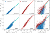 |
Fig. 1. Correlations between the stellar mass, M*, of simulated EAGLE (top row) and TNG (bottom row) galaxies and circular velocities at the stellar half-mass radius, Vc, e, of late-type (S) systems (left column); line-of-sight velocity dispersion, averaged within the stellar effective radius of early-type (E) systems (middle column); and stellar half-mass radius (right column), for all galaxies in the sample. (See Appendix A for details on the morphological classification of simulated galaxies.) In all panels, red circles denote ellipticals, and blue spiral symbols denote spirals. Grey symbols are used to indicate other galaxies of intermediate type. Thick wiggly curves of matching colour indicate the median trends, computed in stellar mass bins. The thick smooth curves are fits used for (or obtained with) the fiducial model described in Sect. 3.3. |
The right column in Fig. 1 shows the relation between effective radius and stellar mass. (This figure also includes all galaxies of intermediate galaxy types, shown in grey.) Unlike the correlations involving velocities, the trends between mass and size are less clear and show much larger scatter; at fixed mass, galaxies have effective radii that span nearly an order of magnitude. There are also significant differences between the radii of EAGLE and TNG galaxies. TNG galaxies span a wider range of radii and, particularly at lower masses, the average radius of both E and S TNG galaxies appear smaller than their EAGLE counterparts.
Why are the EAGLE and TNG velocity correlations in such good agreement if their radii differ? Is the larger scatter in the TNG Tully-Fisher relation related to the larger scatter of S galaxy radii? To answer these questions we need to consider first whether TNG and EAGLE galaxies populate similar dark matter halos.
3.2. The galaxy stellar mass-halo mass relation
This is done in Fig. 2, where we show the galaxy stellar mass versus virial mass relation for both EAGLE (left) and TNG (right) galaxies. Open diamonds (EAGLE) and triangles (TNG) indicate the median M200 (as well as their respective 25 − 75 percentile range) for four thin bins of stellar mass. The ‘abundance-matching’ (AM) relations of Behroozi et al. (2019, hereafter, B+19) and Moster et al. (2018, hereafter, M+18) are also shown, for reference. These AM relations adopt the stellar mass functions of Bernardi et al. (2013, 2017). Ellipticals tend to inhabit, at given M*, more massive halos, a trend that agrees with what is inferred from observed satellite populations or from galaxy lensing analyses (see e.g., Wang & White 2012; Mandelbaum et al. 2016). The difference, however, is slight and does not exceed a factor of ∼2 in either simulation. Ellipticals are also more prevalent at high masses while spirals dominate at lower masses.
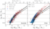 |
Fig. 2. Galaxy stellar mass versus halo virial mass relation. Bottom axes indicate M200 in M⊙; top axes indicate virial velocity, V200, in km s−1. The left-hand panel corresponds to EAGLE, right-hand panel to TNG. Symbols show individual galaxies coloured by morphology: red circles indicate early-type (E); blue spiral symbols denote late-type (S); and grey squares are used for all others. Solid and dashed thick black curves indicate, for reference, the results of abundance-matching models from Behroozi et al. (2019) and Moster et al. (2018), respectively. Open symbols (diamonds for EAGLE, triangles for TNG) indicate median M200 values in the four bins of M* highlighted by the grey horizontal bands (these are used for the model curves shown in Fig. 3). ‘Error bars’ in each symbol denotes the 25–75 percentile range in each bin. Starred coloured symbols correspond to halo masses used for the models discussed in Fig. 9. |
Figure 2 also shows that, at fixed M*, TNG halos have systematically lower mass than EAGLE. The difference, however, is small for M* < 1011 M⊙, with an offset in virial mass of less than a factor of ∼0.25 dex at fixed M*. The difference is more noticeable at higher masses, reaching a virial mass offset of a factor of ∼4 at M* ∼ 3 × 10¹¹ M⊙. Despite these differences, the FJR for massive EAGLE and TNG ellipticals is nearly identical (middle column of Fig. 1). Also somewhat puzzlingly, the halo mass difference between EAGLE and TNG for lower-mass galaxies does not seem enough to account for the enhanced scatter of the TNG Tully-Fisher relation relative to EAGLE.
Since both E and S galaxies inhabit similar halos (at fixed M*) it is important to consider the role of galaxy radii in setting the characteristic velocity of a galaxy. Indeed, both velocity dispersions (for E galaxies) and rotation velocities (for S galaxies) are sensitive to the total mass enclosed within the stellar half-mass radius, re, which we consider next.
3.3. The circular velocity-size plane
In order to analyse ellipticals and discs jointly, we consider for all simulated galaxies the relation between their effective radii, Re, and the circular velocity at the stellar half-mass radius, Vc, e. This is shown in Fig. 3, where the left-hand panel corresponds to EAGLE galaxies and the right-hand panel to TNG. All galaxies are shown in grey but we highlight in colour those in four 0.1 dex-thin stellar mass bins centred at log(M*/M⊙) = 10.1, 10.5, 10.9, and 11.3. (See the grey bands in Fig. 2.) As in other figures, filled circles denote early-type systems and spiral symbols indicate S galaxies.
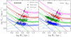 |
Fig. 3. Circular velocity at the stellar half-mass radius, Vc, e, as a function of the effective radius, Re, for EAGLE (left-hand panel) and TNG (right-hand panel) simulated galaxies. All galaxies are shown in grey; those in four thin bins of stellar mass are highlighted in colour (see the grey bands in Fig. 2). Median stellar masses for each bin are listed in the legend. Circles indicate early-type (E) galaxies, spirals denote late-type (S). Slanted dashed lines indicate the expected loci of galaxies that are fully dominated by their stellar component, that is, |
Slanted dashed lines (labelled ‘stars’) indicate the loci expected for systems fully dominated by their stellar component, that is,  , assuming spherical symmetry. Dotted curves (labelled ‘DM’) indicate the dark matter circular velocity profile of NFW halos with virial mass taken from the M* − M200 relation of each simulation (see the open symbols in Fig. 2). The NFW dark halo profiles use concentrations from Ludlow et al. (2016) and are scaled down, at all radii, by the universal baryon fraction, Mdark(r) = (1 − fbar)MNFW(r), with fbar = Ωbar/Ωm = 0.186, as appropriate for a Planck-normalized ΛCDM cosmology. Here, MNFW(r = R200) = M200. The NFW profiles have also been ‘contracted’ to account for the effect of galaxy assembly, following Gnedin et al. (2004).
A simple fiducial model that predicts the loci of galaxies of given stellar mass in this plane may be constructed by adding, in quadrature, the dashed and dotted curves, respectively. This is shown by the solid coloured curves in Fig. 3, where the ‘error bands’ correspond to varying the NFW concentration of each halo by the expected scatter of 0.09 dex (Ludlow et al. 2016). It can be noted that model curves of the same stellar mass differ between EAGLE and TNG; this is due entirely to the slightly different M* − M200 relations of these two simulations (Fig. 2).
At fixed M*, the circular velocity becomes nearly independent of galaxy size for galaxies with effective radii exceeding some ‘critical’ radius, Rcrit. This threshold is reasonably well approximated by the solid black curve in each panel, which tracks, as a function of M*, the effective radius of a galaxy expected, according to the fiducial model, to contain as much dark matter as stars within re (i.e. the radii where the dotted and dashed lines intersect in Fig. 3).
It may be somewhat surprising that ellipticals and spirals of given M* seem to follow approximately the same trends, despite the slight but systematic differences in the M* − M200 relation of galaxies of different morphology highlighted in Fig. 2. This is due to the fact that, for NFW models, the dark mass at fixed radii in the inner regions does not scale linearly with virial mass. Indeed, a M200 = 1012 M⊙ NFW halo of average concentration encloses roughly ∼4.2 × 10⁹ M⊙ within the inner 3 kpc. Varying the virial mass by a factor of two above and below that value leads to variations of less than 20% in the dark mass enclosed within 3 kpc. In other words, even relatively large offsets in the M* − M200 relation may yield nearly imperceptible changes in the scaling relations.
Although we are encouraged by the relatively good agreement between the fiducial model and simulation results, there are systematic differences that are worth highlighting. For example, the model seems to under-predict circular velocities for low-mass galaxies, and to over-predict them for the most massive ones. These velocity offsets are clear, but relatively small, typically of order ∼0.05 dex, but suggest that our fiducial model could be updated to improve agreement. One possibility would be to consider different halo contraction models. After all, there is evidence that massive ellipticals are better modelled by an uncontracted halo (see e.g., Shankar et al. 2017; Shajib et al. 2020). We plan to consider such corrections in future contributions.
3.3.1. Reasons why is the Tully-Fisher relation independent of surface brightness
Despite the simplicity of the fiducial model described above, it does a remarkable job at reproducing the relation between characteristic velocity and galaxy radius. The model shows that, at fixed M*, the characteristic velocity is expected to be roughly independent of galaxy radius for a wide range of radii (i.e. at large enough radii, curves of constant M* are nearly horizontal in Fig. 3). Indeed, only for galaxy radii smaller than the ‘critical’ value, rcrit, the gravitational importance of the stars raises the circular velocity of a system at re over and above the asymptotic velocity of its surrounding halo (see e.g., Mamon & Łokas 2005a,b).
The reason for this is illustrated in Fig. 4, where the solid black curves show schematic circular velocity curves corresponding to a fixed NFW halo (red dashed curve) and a galaxy of fixed stellar mass but varying half-mass radius (shown by the open circles). The galaxies are assumed to be exponential discs, and their contributions to the circular velocity are shown by the blue dotted curves. Because of the shape of the dark halo profile, the circular velocity at the half-mass radius, Vc, e (shown by open circles), barely changes for discs spanning a wide range of radii, between ∼4 and ∼30 kpc. (For clarity, the halo, labelled ‘NFW’, is not ‘contracted’ in this illustration.)
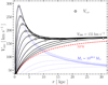 |
Fig. 4. Schematic circular velocity profiles (black solid lines) of galaxies of stellar mass M* = 3 × 10¹⁰ M⊙, embedded in an NFW halo (red dashed curve) of virial mass M200 = 1.4 × 10¹² M⊙ (or, equivalently, V200 = 155 km s−1) and average concentration, c200 = 7.6 (Ludlow et al. 2016). Different curves correspond to exponential stellar discs of varying half-mass radius. The circular velocity of the dark matter plus stars at each of the half-mass radii, Vc, e, is shown by the open circles. It is clear that Vc, e is approximately independent of re for galaxy radii exceeding a ‘critical’ radius (rcrit) of order ∼5 kpc. The characteristic rotation speeds of disc galaxies of given mass are thus roughly independent of radius, provided galaxy radii satisfy re > rcrit. Conversely, galaxies with re < rcrit are expected to be dominated by their stellar component, and their characteristic velocities should depend sensitively on re. |
This is, of course, the main reason why the TFR is ‘independent of surface brightness’ in simulations (Ferrero et al. 2017): The TFR depends solely on M*, and reflects simply the scaling between M* and the characteristic velocity of its surrounding dark halo. The series of models in Fig. 4 also make clear that this independence should break down for galaxy radii smaller than some ‘critical’ radius, which we may define as the galaxy radius for which the contribution to Vc, e of the dark and luminous components is the same. This is the definitions used to compute Rcrit for each of the model curves shown in Fig. 3 and show them as connected coloured diamonds (EAGLE) or triangles (TNG). Clearly, the critical radius increases with stellar mass, and that it is sensitive to the assumed M* − M200 relation. Appendix B provides an analytical expression for the critical radius as a function of stellar mass, which may be useful for the interested reader.
3.3.2. The differences between TNG and EAGLE scaling laws
The results of Fig. 3 may be used to explain the trends and puzzles highlighted when comparing the TFR and FJR of EAGLE and TNG in Fig. 1. We consider first why the TFR in EAGLE exhibits so little scatter, even though late-type galaxy radii span a wide range. This is simply because S galaxies in EAGLE have relatively large radii, which exceed in all cases their corresponding values of Rcrit. As discussed above, in this regime the characteristic velocity is independent of galaxy radius and depends solely on the M* − M200 relation. The scatter in the EAGLE TFR thus reflects the scatter in that relation, which is rather small (see Ferrero et al. 2017, for a more detailed discussion).
The same argument explains why the TNG Tully-Fisher relation has enhanced scatter compared to EAGLE (see the left-hand panels in Fig. 1). This is not because of enhanced scatter in the M* − M200 relation, but rather because spiral galaxy radii in TNG cover a wider range than in EAGLE, and include many systems with radii comparable to, or smaller than, the critical radius for their M*. These galaxies have therefore more dominant stellar components and higher characteristic velocities, as may be seen for systems with re < rcrit in Fig. 4. These ‘small’ galaxies scatter off the TFR towards higher velocities at fixed M*, yielding increased dispersion in the TNG Tully-Fisher relation relative to EAGLE.
One may also use these arguments to explain the invariance of the FJR in EAGLE and TNG (middle column in Fig. 1). This is due to the rough compensation of two effects: TNG ellipticals are smaller on average than EAGLE’s, which pushes their velocities high, but, at fixed M*, they inhabit systematically lower-mass halos, which pushes their velocities down. The combination of the two effects results in FJR relations that are basically indistinguishable for TNG and EAGLE. We shall return to this issue in more detail when comparing with observations in Sect. 4.5.
3.4. A possible new distance indicator
A simple application of these ideas leads to a new secondary distance indicator that may be applied indistinctly to S and E galaxies, by exploiting the unique mapping between the location of a galaxy in the Vc, e − Re plane and its stellar mass. This mapping still holds if we substitute galaxy radii by the mean stellar surface density of a galaxy,  , with the advantage that both velocity and surface density/brightness are independent of distance.
We show this in the left-hand panel of Fig. 5 where all EAGLE galaxies are shown in grey (shaded to indicate stellar mass) and superposed on a grid of models akin to those shown in Fig. 3, but for a finer spacing in stellar mass. Each model curve denotes the loci of constant M*, so that any galaxy in this plane may be assigned a stellar mass interpolated from this grid. Each curve results from varying Re in the fiducial model at fixed M*, assuming a galaxy mass-halo mass relation and contracted halos of average concentration, as described in Sect. 3.3. We show the result of this interpolation in the right-hand panel of Fig. 5, where we compare ‘predicted’ values of the stellar mass with ‘true’ values measured from the simulation. The agreement between the two is remarkable, especially given the simplicity of the model, with little bias and an exceptionally small scatter of only 0.078 dex around the 1:1 relation.
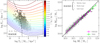 |
Fig. 5. Procedure to use the model as a secondary distance indicator. Left: grid of constant M* model curves linking Vc, e and the mean stellar surface density (brightness) within the effective radius, |
This suggests a secondary distance indicator, where the measurement of a characteristic velocity and an effective surface brightness may be combined to yield a prediction for the total stellar mass. Comparing this to the apparent magnitude of a galaxy would yield its distance in a straightforward way. This secondary distance indicator is, of course, just a combination of (i) the TFR for ‘large’ (typically spiral) galaxies, which have Re > Rcrit (or, equivalently, Σe < Σcrit) and for which the characteristic velocity depends solely on stellar mass (i.e. curves of constant M* are nearly horizontal in Fig. 5 for Σe < Σcrit), and (ii) an FP-like relation for ‘small’ (typically elliptical) galaxies with Re < Rcrit (Σe > Σcrit), for which the characteristic velocity depends on both velocity and stellar surface density/brightness.
It should be noted that the only information used to construct the grid shown in the left-hand panel of Fig. 5 is the EAGLE galaxy stellar mass-halo mass relation and the assumption that ΛCDM halos are well represented by NFW profiles. The same procedure may be applied to TNG, after modifying the model grid to account for the slightly different M* − M200 relation. The results are also shown in the right-hand panel of Fig. 5, with similar results (little bias and a scatter of only 0.075 dex). We shall return to these issues when applying these results to observed galaxies in Sect. 4.
3.5. The ‘tilt’ of the fundamental plane
The analysis of Fig. 3 may also be applied to shed light on the interpretation of a possible ‘tilt’ to the FP. This is commonly used to refer to the fact that the best fitting ‘plane’ for elliptical galaxies in the stellar mass-velocity-radius space differs from that expected from the ‘virial’ relation, M* ∝ σ2Re.
For this scaling to hold, stars must be gravitationally dominant over the dark matter at Re. In the language of Fig. 3, this is equivalent to having galaxies closely hug the dashed curves in this figure, or, equivalently, galaxies with radii much smaller than ‘critical’. Although some such galaxies exist, they are few; most TNG and EAGLE ellipticals straddle radii around the critical value. Their velocities are therefore heavily affected by the dark matter component, leading them to deviate from the dashed lines and, consequently, from the ‘virial’ scaling (see e.g., Zaritsky et al. 2006, for a similar discussion).
In other words, the ‘tilt’ in the simulated FP is related to the fact that, at fixed M*, physically larger galaxies simply contain more dark matter than smaller ones. We show this in Fig. 6 where we plot, for all S and E galaxies in TNG and EAGLE, the ‘dynamical mass-to-light ratio’ as a function of galaxy radius, expressed in units of the ‘critical’ value. This ratio is defined here as that between total mass and stellar mass within re, that is,  . A ratio close to unity thus indicates that stars are fully dominant.
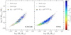 |
Fig. 6. ‘Dynamical mass-to-light ratio’, |

Expressed in this manner, we see in Fig. 6 that the dynamical mass-to-light ratio increases monotonically with Re/Rcrit, for all galaxies, regardless of stellar mass. This insight may in principle be checked observationally as it predicts that subsets of ellipticals that are ‘compact’ (in the sense of Re ≪ Rcrit) should exhibit smaller tilt, and also that the tilt should exist even for ellipticals of fixed stellar mass, provided they span a wide enough range of galaxy radii.
These results also suggest that rotational support is secondary to galaxy size in determining the magnitude of the tilt. Indeed, the coloured symbols in Fig. 6 indicate the importance of rotation (measured by κrot) for galaxies with stellar masses M* = 1010.5 ± 0.05 M⊙ (i.e. green symbols in Fig. 3). For such galaxies, there is no clear-cut indication that rotation plays a major role at fixed galaxy size, although size and rotational support are clearly correlated at fixed M*. Our results thus suggest that the ‘tilt’ should be minimized when considering samples of fixed Re/Rcrit. Choosing ‘slow’ or ‘fast rotators’ should in principle yield samples with systematically low or high Re/Rcrit. This may explain the systematic differences in the FP of slow versus fast rotators reported by Bernardi et al. (2020). We plan to address this issue more directly, and with an enhanced observational sample, in future work.
4. Application to observed galaxies
4.1. Scaling laws
We now apply these ideas to the observed sample (Sect. 2.3), which contains an assortment of galaxies of different morphological types, ranging from massive ellipticals to late-type spirals spanning a wide range of mass. Their scaling laws are presented in Fig. 7, where the left-hand panel shows the TF relation of disc galaxies and the middle panel shows the FJR for ellipticals. It should be noted that both are rather tight relations, with a mass scatter of 0.28 dex and 0.27 dex, respectively, about the median velocity trends traced by the thick wiggly curves in each panel.
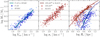 |
Fig. 7. Correlations between the stellar mass of galaxies in our observational sample and disc rotation speed at the stellar half-mass radius (disc galaxies from SPARC and P+07, left-hand panel); line-of-sight velocity dispersion, averaged within the stellar half-mass radius (ellipticals from ATLAS3D and SLACS; middle panel); and effective radius (all galaxies; right-hand panel). Circles denote ellipticals, spiral symbols denote discs. The thick wiggly curves indicate the median trend, computed in bins of stellar mass. The smooth coloured curves in the right-hand panel indicate fits to the average trends. |
As for simulated galaxies, the mass-size relation (right-hand panel in Fig. 7) exhibits much larger scatter, spanning nearly a decade in galaxy radius at fixed M*. Still, there are strong trends once the sample is parsed into morphological types, and it is clear that the average size increases with increasing mass for both early and late types.
It is also clear from comparing Figs. 7 and 1 that there are strong similarities between the scaling laws of observed and simulated galaxies. This motivates us to carry out the same analysis as in the previous section, where, in order to compare galaxies of different morphologies, we estimate their total mass (or, equivalently, circular velocity) enclosed within the stellar half-mass radius, re. In the case of spirals, assuming that the rotation speed at re traces the circular velocity seems reasonable, in other words, Vc, e ≡ Vrot. For elliptical galaxies this is less straightforward, but there is compelling literature arguing that the line-of-sight velocity dispersion may also be used as a tracer of the circular velocity at re (see e.g., Walker et al. 2009; Wolf et al. 2010, and references therein).
We show this in Fig. 8 for all E galaxies in EAGLE (open circles) and TNG (filled circles). Red solid and dashed lines indicate power-law fits to the σe − Vc, e relation, with circular velocity RMS of 0.05 dex and 0.07 dex, respectively. The solid black line indicates the result of the model of Wolf et al. (2010),  , which provides a less accurate but acceptable fit to the combined data, with an RMS of 0.12 dex. For simplicity, we shall hereafter adopt this relation in order to estimate Vc, e for observed ellipticals in our sample, although one could in principle improve on this prescription by using a more sophisticated analysis (see e.g., Courteau et al. 2014, for a review).
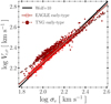 |
Fig. 8. Circular velocity at the stellar half-mass radius, Vc, e as a function of the stellar line-of-sight velocity dispersion, averaged within the effective radius, Re. All galaxies categorized as early-type in EAGLE (open circles) and TNG (filled circles) are shown. (See Appendix A for details on the morphological classification procedure.) The thick black solid line indicates the model of Wolf et al. (2010). The solid and dashed red lines are simple power-law fits to the EAGLE and TNG data, respectively. For fits of the form Vc, e = V0 (σe/km s−1)n, the best fit parameters are (V0, n) = (2.37 km s−1, 0.94) for EAGLE and (V0, n) = (7.03 km s−1, 0.73) for TNG. |
4.2. The circular velocity-size plane
The assumption that  enables us to place all observed galaxies in the Vc, e versus Re plane, as shown in Fig. 9. Following a similar analysis to that adopted when discussing Fig. 3, we highlight in colour galaxies in three thin bins of stellar mass (the bins are indicated by shaded grey bands in Fig. 7). Reassuringly, we see the same qualitative behaviour as for simulated galaxies, albeit with increased scatter. The trends are well reproduced by the same fiducial model introduced in Sect. 3.3, after assuming a halo virial mass for each of the three bins.
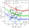 |
Fig. 9. Same as Fig. 3, but for observed galaxies in our sample. Circular velocities, Vc, e, are assumed to be equal to the characteristic rotation speed for galaxy discs (spiral symbols in Fig. 7) and are inferred from the Wolf et al. (2010) relation for ellipticals (circles). Halo masses for each of the three stellar mass bins highlighted in coluor are chosen from the M+18 abundance-matching relation, as shown by the starred symbols in Fig. 2. Coloured stars joined by a solid line indicate the ‘critical’ radius where the dark matter and stellar mass within the stellar half-mass radius are equal. |
For the three bins of stellar mass centred at log M*/M⊙ = 10.1, 10.6, and 11.1, halo masses of log M200/M⊙ = 11.56, 12.1, and 13.28 result in adequate fits for both elliptical and spiral galaxies in each bin. (As in Fig. 3 the coloured bands show the result of the fiducial model, including a variation of 0.09 dex in the NFW concentration). These halo mass values are shown as starred symbols in Fig. 2, and have been chosen to lie on the M+18 abundance-matching relation. The agreement is encouraging, for it implies that, as in the simulations, the data seem consistent with the idea that there are, at fixed M*, no major differences between the velocity-radius relation of galaxies of different morphological types.
4.3. The circular velocity-surface brightness plane as distance indicator
We can take the modelling one step further, and, as in Fig. 5, we can use ‘predict’ stellar masses based on the location of galaxies in the Vc, e − Σe plane, together with an assumed M* − M200 relation and a halo contraction model. We show the grid of ‘fiducial’ models (see Sect. 3.3) in the left-hand panel of Fig. 10 that result from assuming the M+18 abundance-matching relation. The ‘predicted versus true’ stellar masses are shown in the right-hand panel of the same figure, and show encouraging results. The predicted masses show overall little bias (predicted masses are on average just ∼0.1 dex higher than observed) and an RMS of only 0.19 dex about the 1:1 relation.
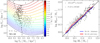 |
Fig. 10. Same as Fig. 5, but for our observed galaxy sample. The panel on the left shows the grid of stellar mass models computed using the fiducial model described in Sect. 3.4, assuming the M+18 abundance-matching M* − M200 relation. Line colours indicate stellar mass, as indicated in the colour bar. Observed galaxies are shown by symbols in shades of grey, according to their stellar mass. Circles are used for early-types; spiral symbols for late types. Interpolation on this model grid allows stellar masses to be ‘predicted’ solely from the location of a galaxy in the Vc, e − Σe plane. The predicted values of M* are shown as a function of the true values of M* in the right-hand panel. The median trend is shown by the thick pink line, with an ‘error band’ that spans the change in the median predicted values after varying the M* − M200 relation by a factor of two in halo mass above and below the M+18 relation. The blue curve shows the median trend, but for a model that includes ‘adiabatic’ contraction instead of the Gnedin et al. (2004) contraction model. |
The agreement between predicted and observed stellar masses may be improved by adopting a different M* − M200 relation, or by refining the very simple model used to construct the grid shown in the left-hand panel of Fig. 10. Interestingly, the results are fairly insensitive to changes in the M* − M200 relation. Indeed, the pink ‘error band’ shows the effect on the median trend of varying by a factor of two (above and below) all halo masses around the M+18 relation. Varying halo masses by a factor of four in this manner has little effect on the model grid and, as a consequence, on the predicted masses. This is a result of the weak dependence on halo virial mass of the dark mass enclosed in the inner regions discussed in Sect. 3.3.
Predicted stellar masses are more sensitive to the halo ‘contraction’ model assumed to take into account the halo response to the assembly of the galaxy. Our fiducial model assumes the Gnedin et al. (2004) contraction, which has been shown to reproduce fairly accurately the results of cosmological hydrodynamical simulations (see e.g., Schaller et al. 2015; Cautun et al. 2020). The ‘adiabatic’ contraction model of Blumenthal et al. (1986), on the other hand, yields lower predicted masses and better agreement overall with the observed M*, as shown by the blue thick line in the right-hand panel of Fig. 10. Indeed, the scatter about the median ‘adiabatic’ curve is just 0.17 dex.
The scatter in the predicted versus true stellar mass quoted above is actually comparable to the mass scatter about the median TFR shown in the left-hand panel of Fig. 7, which is 0.28 dex for the combined P+07 and SPARC samples. This implies that the grid model in Fig. 10 may be used, in principle, as a competitive secondary-distance indicator applicable to galaxies of all morphologies and that only relies on distance-independent kinematic and surface brightness measures. Further work would be needed to express this idea in explicit observational terms, a task that we defer to future work.
4.4. The ‘tilt’ of the observed fundamental plane
We consider next whether the ‘tilt’ in the FP of E galaxies correlates with the size of the galaxy, expressed in terms of the ‘critical radius’ introduced in Sect. 3.5. This is shown in Fig. 11, which indicates that, as for simulated galaxies, the ‘dynamical mass-to-light ratio’ of observed galaxies does indeed correlate with Re/Rcrit, although with larger scatter. At fixed M*, galaxies with larger effective radii enclose more dark matter than smaller galaxies and tend to have higher values of Mdyn, e/(M*/2). As in Fig. 6, there is a smooth transition between spirals and ellipticals at fixed M*. This result offers a simple and intuitive explanation for the origin of the ‘tilt’ in the FP, as discussed in Sect. 3.5.
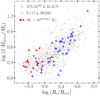 |
Fig. 11. Same as Fig. 6, but for observed galaxies in our sample. Critical radii are computed as a function of M* using our fiducial model and the M+18 M* − M200 relation. Grey symbols denote all observed galaxies in our analysis while red and blue correspond to S and E galaxies, respectively, with stellar masses M* = 1010.5 ± 0.1 M⊙. It should be noted that the dynamical mass-to-light ratio increases with increasing galaxy size, at fixed M*. The mass-to-light ratio ratios also increase, in general, with increasing galaxy stellar mass because massive ellipticals tend to have larger values of Re/Rcrit than less massive early-type systems. As for simulated ellipticals, the ‘tilt’ of the FP appears correlate strongly with galaxy size. |
4.5. Comparison between simulated and observed scaling laws
We end our discussion by comparing the scaling laws of observed and simulated galaxies. These are shown in Fig. 12, where the top and bottom rows display, as in Fig. 7, the observed correlations between galaxy radius, stellar mass, and characteristic velocity, split by morphological type (top row for spirals, bottom row for ellipticals).
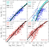 |
Fig. 12. Comparison of observed and simulated galaxy scaling laws. Top row corresponds to late-type systems; bottom row to early types. In each panel, symbols denote observed galaxies. The smooth coloured lines represent the median trend of the simulation results, as in Fig. 1. It should be noted that simulations match reasonably well the rotation velocity-stellar mass (TFR; top left-hand panel). The bottom left-hand panel shows line-of-sight velocity dispersions for E galaxies versus stellar mass (FJR). Simulated galaxies have systematically lower (∼0.1 dex) velocities than observed ellipticals. Thick black lines correspond to the fiducial model applied to the hypothetical simulation discussed in Sect. 4.5. The thin black line in the right-hand panels indicate the ‘critical’ radius as a function of M* for the hypothetical simulation. See the discussion in text. |
The smooth coloured lines show the results of our fiducial model applied to each of the simulations. The models use as input, for each simulation, fits to (i) the galaxy stellar mass-halo mass relation (Fig. 2); (ii) the stellar mass-effective radius relation (right-hand panels of Fig. 1); and (for ellipticals) (iii) the relation needed to translate Vc, e into σe (Fig. 8). Details on these fits are provided in Appendix B.
The results of the model are shown by the smooth coloured curves in the left and middle columns of Fig. 1, where they are seen to provide an excellent description of the simulation results. Because of this agreement, and to keep the discussion simple, we shall use these models to discuss the comparison of the simulations with observed data in Fig. 12.
The top left-hand panel of Fig. 12 shows that both simulations do a reasonably good job at reproducing the observed TFR. Following our earlier discussion, this agreement is actually expected, and results because the half-mass radii of simulated spirals are comparable or larger than their ‘critical radius’. In this regime, Vc, e becomes insensitive to galaxy radii, and the TFR depends solely on the M* − M200 relation. The good agreement between observed and simulated TFR thus indicates that TNG and EAGLE spirals are ‘large enough’, and inhabit halos of the ‘right’ mass (Ferrero et al. 2017).
The comparison of the simulated FJR with observed ellipticals is shown in the bottom left-hand panel of Fig. 12. The median trend of both simulations (coloured lines) is similar, but they appear to be offset, on average, by ∼0.1 dex in velocity from the observed FJR. This is intriguing, especially given the excellent agreement between the simulated and observed TFRs.
The reasons for the FJR offset are easier to appreciate by using the same fiducial model to predict the scaling laws expected for a hypothetical simulation that reproduces (i) the abundance-matching galaxy stellar mass-halo mass relation of either M+18 or B+19 (Fig. 2); (ii) the observed galaxy mass-size relations of ellipticals or spirals (see the solid black curve fits in the right-hand panels of Fig. 12); and (iii) the Wolf et al. (2010)Vc, e − σe relation (solid line in Fig. 8).
The resulting model Tully-Fisher and Faber-Jackson relations are shown with black curves in the left-hand panels of Fig. 12. It is clear from these panels that the hypothetical simulation improves the agreement with observation in both cases. This suggests that the offset in the FJR is related to differences in at least one of the three model inputs listed above between the hypothetical simulation and TNG or EAGLE.
For example, compared to the hypothetical simulation model, low-mass EAGLE ellipticals (say, M* ∼ 1010 M⊙) have similar halo masses but much larger sizes than observed. Massive EAGLE ellipticals (say, M* ∼ 1011.5 M⊙), on the other hand, have similar sizes but much lower halo masses. Either or both of these effects lead to lower velocity dispersions, which explains the offset between the observed and simulated FJRs over the whole mass range. Although the details differ, similar reasoning may also be used to explain readily the FJR offset of TNG ellipticals.
Interestingly, for massive ellipticals, this analysis leads to a conclusion that applies to both simulations. In this regime, the FJR offset arises both in TNG and EAGLE because massive galaxies form in halos less massive than suggested by abundance-matching models. Indeed, as may be seen from Fig. 2, an elliptical galaxy with stellar mass M∗ ∼ 3 × 10¹¹ M⊙ forms in a halo with virial mass M200 ∼ 5 × 10¹³ M⊙ in EAGLE, or M200 ∼ 3 × 10¹³ M⊙ halo in TNG. Massive simulated galaxies thus form in halos less massive than expected from AM relations, which predict halos ar least as massive as ∼1014 M⊙ for such galaxies. The high velocity dispersion of massive ellipticals thus suggest that simulations like EAGLE or TNG need further adjustments in order to prevent massive galaxies from forming in halos less massive than suggested by abundance-matching analysis.
Our study is not the first to highlight the differences between observed and simulated ellipticals. Lu et al. (2020), for example, have already argued that fitting in detail the FP of ellipticals requires some modifications to simulations like TNG. Our analysis confirms and extends their conclusion, and suggests that only simulations that match closely and simultaneously the abundance-matching M* − M200 relation as well as the observed sizes of galaxies of different morphologies will be able to match their observed scaling laws.
5. Summary and conclusions
We have used ΛCDM cosmological hydrodynamical simulations from the IllustrisTNG and EAGLE projects to study the scaling laws that relate galaxy stellar mass with the characteristic size and velocity of luminous (M* > 1010 M⊙) galaxies of different morphologies. These simulations evolve volumes large enough to yield statistically significant samples of luminous galaxies and have numerical resolution high enough to allow for the identification of galaxies of different morphologies (including rotation-dominated ‘spirals’ and dispersion-dominated ‘ellipticals’) and for the measurement of their characteristic sizes and velocities.
The simulations, partly by design, match approximately the galaxy mass-halo mass relation predicted from abundance-matching analysis such as those of Moster et al. (2018) and Behroozi et al. (2019). Simulated ellipticals and spirals show little difference in this regard; at given M*, both morphological types inhabit halos of similar virial mass. Differences in their scaling laws thus result mainly from differences in size (ellipticals are systematically smaller than spirals) and, consequently, in dark matter content (smaller galaxies enclose less dark mass within their effective radii).
Our analysis indicates that, for given M*, there is a ‘critical’ radius that separates galaxies whose characteristic velocities simply trace the characteristic velocity of their surrounding halo (i.e. those with Re > Rcrit, typically spirals) from those where mass and size play a role in setting a galaxy’s characteristic velocity (i.e. those with Re < Rcrit, typically ellipticals).
This suggests a simple interpretation for why the TFR of spiral galaxies is independent of galaxy radius or surface brightness, and for the ‘tilt’ of the FP. The latter, in particular, results from the non-negligible dark matter contribution to dynamical mass estimates. The dark matter content depends directly on the ratio Re/Rcrit, implying that the FP tilt is primarily driven by galaxy ‘size’ rather than mass.
A simple fiducial model that combines the NFW-like structure of ΛCDM halos with the M* − M200 relation of each simulation is able to reproduce well the scaling laws of simulated galaxies. The same fiducial model suggests how scaling laws may be unified into a simple scenario where galaxy stellar mass is determined uniquely by its effective radius, Re, and its circular velocity at the stellar half-mass radius, Vc, e, regardless of morphology.
The model depends only on the assumed M* − M200 relation, and implies that a secondary distance indicator may be constructed by combining two distance independent quantities, the circular velocity, Vc, e, and the effective surface brightness, Σe, to predict the total stellar mass of a galaxy. This distance indicator is remarkably precise, with little bias and a stellar mass (luminosity) scatter of only 0.076 dex for TNG and 0.078 dex for EAGLE.
The analysis discussed above for TNG and EAGLE may also be applied to observational data to provide a cosmological interpretation for the observed galaxy scaling laws and to elucidate the reasons for differences that may arise when confronting simulations with observation. Overall, observed scaling laws seem broadly consistent with the interpretive framework proposed by the simulations. In particular, the interpretation of both the ‘tilt’ of the FP and of the surface brightness independence of the TFR as related to galaxy size seem consistent with the data. Even the unified Vc, e − Σe distance indicator, applied to a galaxy sample that includes galaxies of all morphological types, gives competitive results, with little bias and a stellar mass (luminosity) scatter of 0.17 − 0.19 dex.
Comparing observations with simulations, the few differences that arise can be traced to deviations from either the observed galaxy mass-size relations, or from the abundance-matching galaxy stellar mass-halo mass relation. A hypothetical ΛCDM simulation where those two requirements are closely and simultaneously met seems broadly consistent with the relations linking the size, mass, and kinematics of galaxies of all morphological types. This should be rightly regarded as a major success of the ΛCDM model in the highly non-linear regime of the inner regions of individual galaxies.
Virial quantities are identified by a ‘200’ subscript and measured at the virial radius, r200, defined as the radius where the enclosed mean density is 200 times the critical density of the Universe, ρcrit = 3H2(z)/8πG.
This use of the term ‘virial’ differs from that used in a cosmological context (Eq. (1)). We shall distinguish between the two by referring to masses inferred from M ∝ σ2R as dynamical or ‘virial’, in quotation marks.
Acknowledgments
We thank Laura Sales for useful comments and Isabel Santos Santos for providing the SPARC data used in this study in electronic form. M. G. A, J. A. B and I. F acknowledge financial support from CONICET through PIP 11220170100527CO grant.
References
- Aquino-Ortíz, E., Sánchez, S. F., Valenzuela, O., et al. 2020, ApJ, 900, 109 [Google Scholar]
- Auger, M. W., Treu, T., Bolton, A. S., et al. 2010, ApJ, 724, 511 [Google Scholar]
- Barat, D., D’Eugenio, F., & Colless, M., et al. 2019, MNRAS, 487, 2924 [Google Scholar]
- Behroozi, P., Wechsler, R. H., Hearin, A. P., & Conroy, C. 2019, MNRAS, 488, 3143 [Google Scholar]
- Bell, E. F., & de Jong, R. S. 2001, ApJ, 550, 212 [NASA ADS] [CrossRef] [Google Scholar]
- Bell, E. F., McIntosh, D. H., Katz, N., & Weinberg, M. D. 2003, ApJS, 149, 289 [Google Scholar]
- Bernardi, M., Sheth, R. K., Annis, J., et al. 2003, AJ, 125, 1866 [Google Scholar]
- Bernardi, M., Meert, A., Sheth, R. K., et al. 2013, MNRAS, 436, 697 [Google Scholar]
- Bernardi, M., Meert, A., Sheth, R. K., et al. 2017, MNRAS, 467, 2217 [Google Scholar]
- Bernardi, M., Domínguez Sánchez, H., Margalef-Bentabol, B., Nikakhtar, F., & Sheth, R. K. 2020, MNRAS, 494, 5148 [Google Scholar]
- Blanton, M. R., & Roweis, S. 2007, AJ, 133, 734 [Google Scholar]
- Blumenthal, G. R., Faber, S. M., Flores, R., & Primack, J. R. 1986, ApJ, 301, 27 [Google Scholar]
- Bolton, A. S., Burles, S., Koopmans, L. V. E., Treu, T., & Moustakas, L. A. 2006, ApJ, 638, 703 [Google Scholar]
- Bullock, J. S., Kolatt, T. S., Sigad, Y., et al. 2001, MNRAS, 321, 559 [Google Scholar]
- Bundy, K., Bershady, M. A., Law, D. R., et al. 2015, ApJ, 798, 7 [NASA ADS] [CrossRef] [Google Scholar]
- Cappellari, M., Bacon, R., Bureau, M., et al. 2006, MNRAS, 366, 1126 [NASA ADS] [CrossRef] [Google Scholar]
- Cappellari, M., Scott, N., Alatalo, K., et al. 2013a, MNRAS, 432, 1709 [NASA ADS] [CrossRef] [Google Scholar]
- Cappellari, M., McDermid, R. M., Alatalo, K., et al. 2013b, MNRAS, 432, 1862 [Google Scholar]
- Cautun, M., Benítez-Llambay, A., Deason, A. J., et al. 2020, MNRAS, 494, 4291 [Google Scholar]
- Chabrier, G. 2003, PASP, 115, 763 [Google Scholar]
- Ciotti, L., Lanzoni, B., & Renzini, A. 1996, MNRAS, 282, 1 [Google Scholar]
- Conselice, C. J., Bundy, K., Ellis, R. S., et al. 2005, ApJ, 628, 160 [Google Scholar]
- Cortese, L., Fogarty, L. M. R., Ho, I. T., et al. 2014, ApJ, 795, L37 [Google Scholar]
- Courteau, S., & Rix, H.-W. 1999, ApJ, 513, 561 [Google Scholar]
- Courteau, S., Dutton, A. A., van den Bosch, F. C., et al. 2007, ApJ, 671, 203 [NASA ADS] [CrossRef] [Google Scholar]
- Courteau, S., Cappellari, M., de Jong, R. S., et al. 2014, Rev. Mod. Phys., 86, 47 [NASA ADS] [CrossRef] [Google Scholar]
- Crain, R. A., Schaye, J., Bower, R. G., et al. 2015, MNRAS, 450, 1937 [NASA ADS] [CrossRef] [Google Scholar]
- Desmond, H., & Wechsler, R. H. 2017, MNRAS, 465, 820 [Google Scholar]
- de Zeeuw, P. T., Bureau, M., Emsellem, E., et al. 2002, MNRAS, 329, 513 [NASA ADS] [CrossRef] [Google Scholar]
- Djorgovski, S., & Davis, M. 1987, ApJ, 313, 59 [Google Scholar]
- Dolag, K., Borgani, S., Murante, G., & Springel, V. 2009, MNRAS, 399, 497 [Google Scholar]
- Dressler, A., Lynden-Bell, D., Burstein, D., et al. 1987, ApJ, 313, 42 [Google Scholar]
- Dutton, A. A., van den Bosch, F. C., Faber, S. M., et al. 2011, MNRAS, 410, 1660 [NASA ADS] [Google Scholar]
- Faber, S. M., & Jackson, R. E. 1976, ApJ, 204, 668 [NASA ADS] [CrossRef] [Google Scholar]
- Faber, S. M., Dressler, A., Davies, R. L., et al. 1987, in Nearly Normal Galaxies. From the Planck Time to the Present, ed. S. M. Faber, et al., 175 [Google Scholar]
- Ferrero, I., Abadi, M. G., Navarro, J. F., Sales, L. V., & Gurovich, S. 2012, MNRAS, 425, 2817 [Google Scholar]
- Ferrero, I., Navarro, J. F., Abadi, M. G., et al. 2017, MNRAS, 464, 4736 [Google Scholar]
- Flores, H., Hammer, F., Puech, M., Amram, P., & Balkowski, C. 2006, A&A, 455, 107 [NASA ADS] [CrossRef] [EDP Sciences] [Google Scholar]
- Gallazzi, A., Charlot, S., Brinchmann, J., & White, S. D. M. 2006, MNRAS, 370, 1106 [Google Scholar]
- Gerhard, O., Kronawitter, A., Saglia, R. P., & Bender, R. 2001, AJ, 121, 1936 [Google Scholar]
- Gnedin, O. Y., Kravtsov, A. V., Klypin, A. A., & Nagai, D. 2004, ApJ, 616, 16 [Google Scholar]
- Graham, A., & Colless, M. 1997, MNRAS, 287, 221 [Google Scholar]
- Guo, Q., White, S., Li, C., & Boylan-Kolchin, M. 2010, MNRAS, 404, 1111 [NASA ADS] [Google Scholar]
- Jorgensen, I., Franx, M., & Kjaergaard, P. 1996, MNRAS, 280, 167 [Google Scholar]
- Kassin, S. A., Weiner, B. J., Faber, S. M., et al. 2007, ApJ, 660, L35 [NASA ADS] [CrossRef] [Google Scholar]
- Lagos, C. d. P., Schaye, J., Bahé, Y., et al. 2018, MNRAS, 476, 4327 [Google Scholar]
- Lelli, F., McGaugh, S. S., & Schombert, J. M. 2016, AJ, 152, 157 [Google Scholar]
- Lu, S., Xu, D., Wang, Y., et al. 2020, MNRAS, 492, 5930 [Google Scholar]
- Ludlow, A. D., Bose, S., Angulo, R. E., et al. 2016, MNRAS, 460, 1214 [Google Scholar]
- Mamon, G. A., & Łokas, E. L. 2005a, MNRAS, 362, 95 [Google Scholar]
- Mamon, G. A., & Łokas, E. L. 2005b, MNRAS, 363, 705 [Google Scholar]
- Mandelbaum, R., Wang, W., Zu, Y., et al. 2016, MNRAS, 457, 3200 [Google Scholar]
- McAlpine, S., Helly, J. C., Schaller, M., et al. 2016, Astron Comput., 15, 72 [Google Scholar]
- Miller, S. H., Bundy, K., Sullivan, M., Ellis, R. S., & Treu, T. 2011, ApJ, 741, 115 [NASA ADS] [CrossRef] [Google Scholar]
- Mo, H. J., Mao, S., & White, S. D. M. 1998, MNRAS, 295, 319 [Google Scholar]
- Mo, H., van den Bosch, F. C., & White, S. 2010, Galaxy Formation and Evolution (UK: Cambridge University Press) [Google Scholar]
- Moster, B. P., Somerville, R. S., Maulbetsch, C., et al. 2010, ApJ, 710, 903 [Google Scholar]
- Moster, B. P., Naab, T., & White, S. D. M. 2018, MNRAS, 477, 1822 [NASA ADS] [CrossRef] [Google Scholar]
- Navarro, J. F. 2019, Astrophys. Space Sci. Proc., 56, 103 [Google Scholar]
- Navarro, J. F., & Steinmetz, M. 2000, ApJ, 538, 477 [NASA ADS] [CrossRef] [Google Scholar]
- Navarro, J. F., Frenk, C. S., & White, S. D. M. 1996, ApJ, 462, 563 [Google Scholar]
- Navarro, J. F., Frenk, C. S., & White, S. D. M. 1997, ApJ, 490, 493 [NASA ADS] [CrossRef] [Google Scholar]
- Nelson, D., Springel, V., Pillepich, A., et al. 2019, Comput. Astrophys. Cosmol., 6, 2 [Google Scholar]
- Oh, S., Colless, M., Barsanti, S., et al. 2020, MNRAS, 495, 4638 [Google Scholar]
- Ouellette, N. N. Q., Courteau, S., Holtzman, J. A., et al. 2017, ApJ, 843, 74 [Google Scholar]
- Pillepich, A., Springel, V., Nelson, D., et al. 2018, MNRAS, 473, 4077 [Google Scholar]
- Pizagno, J., Prada, F., Weinberg, D. H., et al. 2007, AJ, 134, 945 [NASA ADS] [CrossRef] [Google Scholar]
- Planck Collaboration I. 2014, A&A, 571, A1 [NASA ADS] [CrossRef] [EDP Sciences] [Google Scholar]
- Rosito, M. S., Tissera, P. B., Pedrosa, S. E., & Lagos, C. D. P. 2019, A&A, 629, L3 [CrossRef] [EDP Sciences] [Google Scholar]
- Sales, L. V., Navarro, J. F., Schaye, J., et al. 2010, MNRAS, 409, 1541 [Google Scholar]
- Sales, L. V., Navarro, J. F., Theuns, T., et al. 2012, MNRAS, 423, 1544 [Google Scholar]
- Sánchez, S. F., Kennicutt, R. C., Gil de Paz, A., et al. 2012, A&A, 538, A8 [NASA ADS] [CrossRef] [EDP Sciences] [Google Scholar]
- Scannapieco, C., Wadepuhl, M., Parry, O. H., et al. 2012, MNRAS, 423, 1726 [Google Scholar]
- Schaller, M., Frenk, C. S., Bower, R. G., et al. 2015, MNRAS, 451, 1247 [Google Scholar]
- Schaye, J., Crain, R. A., Bower, R. G., et al. 2015, MNRAS, 446, 521 [Google Scholar]
- Scott, N., van de Sande, J., Croom, S. M., et al. 2018, MNRAS, 481, 2299 [Google Scholar]
- Shajib, A. J., Treu, T., Birrer, S., & Sonnenfeld, A. 2020, MNRAS, submitted [arXiv: 2008.11724] [Google Scholar]
- Shankar, F., Sonnenfeld, A., Mamon, G. A., et al. 2017, ApJ, 840, 34 [Google Scholar]
- Shen, S., Mo, H. J., White, S. D. M., et al. 2003, MNRAS, 343, 978 [NASA ADS] [CrossRef] [Google Scholar]
- Simard, L., Mendel, J. T., Patton, D. R., Ellison, S. L., & McConnachie, A. W. 2011, ApJS, 196, 11 [NASA ADS] [CrossRef] [Google Scholar]
- Springel, V. 2010, MNRAS, 401, 791 [NASA ADS] [CrossRef] [Google Scholar]
- Springel, V., Yoshida, N., & White, S. D. M. 2001, New Astron., 6, 79 [Google Scholar]
- Springel, V., Pakmor, R., Pillepich, A., et al. 2018, MNRAS, 475, 676 [NASA ADS] [CrossRef] [Google Scholar]
- Steinmetz, M., & Navarro, J. F. 1999, ApJ, 513, 555 [NASA ADS] [CrossRef] [Google Scholar]
- Taranu, D., Dubinski, J., & Yee, H. K. C. 2015, ApJ, 803, 78 [Google Scholar]
- Trujillo, I., Burkert, A., & Bell, E. F. 2004, ApJ, 600, L39 [Google Scholar]
- Tully, R. B., & Fisher, J. R. 1977, A&A, 500, 105 [Google Scholar]
- van de Sande, J., Lagos, C. D. P., Welker, C., & Bland-Hawthorn, J., et al. 2019, MNRAS, 484, 869 [Google Scholar]
- Walker, M. G., Mateo, M., Olszewski, E. W., et al. 2009, ApJ, 704, 1274 [NASA ADS] [CrossRef] [Google Scholar]
- Wang, W., & White, S. D. M. 2012, MNRAS, 424, 2574 [Google Scholar]
- Weiner, B. J., Willmer, C. N. A., Faber, S. M., et al. 2006, ApJ, 653, 1027 [NASA ADS] [CrossRef] [Google Scholar]
- Wolf, J., Martinez, G. D., Bullock, J. S., et al. 2010, MNRAS, 406, 1220 [NASA ADS] [Google Scholar]
- Zaritsky, D., Gonzalez, A. H., & Zabludoff, A. I. 2006, ApJ, 638, 725 [Google Scholar]
- Zwaan, M. A., van der Hulst, J. M., de Blok, W. J. G., & McGaugh, S. S. 1995, MNRAS, 273, L35 [NASA ADS] [Google Scholar]
Appendix A: Morphological classification of simulated galaxies
Motivated in part by the fact that our main conclusions are applicable to all simulated galaxies, regardless of morphology, we adopt here a very simple classification procedure that takes into account only the rotational support of the stellar component and the gas content of a galaxy. The first parameter gauges the presence of a stellar disc and its relative prominence; the second parameter is a proxy for recent or ongoing star formation, which also typically occurs in a disc.
Rotational support is measured by the fraction of kinetic energy invested in ordered rotation (Sales et al. 2012):
 (A.1)
(A.1)
The parameter κrot approaches unity for systems with perfect circular motions (disc-dominated) and approaches zero for non-rotating pressure supported spheroidal systems. This parameter is a simple quantitative measure of morphology and correlate extremely well with the fraction of stars with circularity parameters ϵj > 0.5 (commonly used criterion for morphological classification). This parameter was exhaustively analysed in Ferrero et al. (2012), where a cutoff value of κrot = 0.6 was found to best separate discs from spheroids.
The second parameter is the ratio between gas and stellar mass within the galactic radius, rgal, fgas = Mgas/M*. The cutoff value adopted for this parameter is fgas = 0.1. This parameter correlates well with the specific star formation rate, sSFR, in both simulations.On average a galaxy with fgas = 0.1 has log sSFR = −10.5 yr−1. We decided to use the gas mass fraction instead of the sSFR because using the latter yields a large number of E galaxies with low sSFR but substantial amounts of gas.
To summarize, the morphological classification is performed by combining the kinematic parameter κrot with the content parameter Mgas/M*. Galaxies with κrot < 0.6 and Mgas/M* < 0.1 are flagged as early-type. On the other hand, late-type galaxies are those with κrot > 0.6 and Mgas/M* > 0.1.
Figure A.1 shows the gas mass fraction as a function of κrot, EAGLE in the left-hand panel and TNG in the right. Blue spiral symbols and red circles denote galaxies selected as late-type and early-type, respectively. Grey squares indicate galaxies that do not meet both parameters at the same time, which we label as intermediate types.
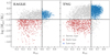 |
Fig. A.1. Gas mass fraction within rgal as a function of the rotational-to-total kinematic energy parameter, κrot. The left-hand panel corresponds to EAGLE, right-hand panel to TNG. Symbols show individual galaxies coloured by morphology: Red circles indicate early-type (E); blue spiral symbols denote late-type (S); grey squares are used for all others. Vertical and horizontal lines denotes cutoff values for morphological classification: κrot = 0.6 and Mgas/M* = 0.1, respectively. |
Appendix B: Model fits
The fits to the median trends of the stellar mass M*, as a function of the half-mass radius, Re shown in the right-hand panels of Fig. 12 follow a polynomial of degree two: log M* = a log  log Re + c. The values of a, b and c for, simulated and observed S and E galaxies may be found in Table B.1.
Parameter values for fits used for M*(M200) and log M*(log Re).
For the galaxy mass-halo mass relation, M*(M200), for observations we asume fits to the M+18 or B+19 (solid and dashed black lines on Fig. 2) curves following the function proposed in Moster et al. (2010):
![Mathematical equation: $$ \begin{aligned} \frac{M_*}{M_{200}} = 2 A \left[ \left(\frac{M_{200}}{M_1}\right)^{-\beta } + \left(\frac{M_{200}}{M_1}\right)^{\gamma } \right]. \end{aligned} $$](/articles/aa/full_html/2021/04/aa39839-20/aa39839-20-eq16.gif) (B.1)
(B.1)
Table B.1 shows the values of A, M1, β and γ appropriate for the EAGLE and TNG simulations. For clarity, these fits are not shown in Fig. 2, but they follow the corresponding open symbols in that figure.
Finally, we provide an analytical expression for the critical radius, Rcrit dependence on M*. To model Rcrit a relation between stellar mass and halo mass as well as a halo contraction model need to be assumed. Table B.2 shows the parameters of a polynomial fit of degree two: log Rcrit = a log  log M* + c. The fits shown in Table B.2 assume a Gnedin et al. (2004) contraction and are valid for M* > 109.5 M⊙.
Parameter values for fits used for log Rcrit(log M*).
As an extra resource for the interested reader we provide on GitHub5 a code that builds the grids shown in Fig. 5 and Fig. 10. More generally, the code returns the predicted stellar mass by providing the surface brightness, Σe, and the effective radii, Re. The code also allows different stellar to halo mass relations (EAGLE, TNG, M+18 or B+19) and different models for the halo contraction (see e.g., Gnedin et al. 2004; Blumenthal et al. 1986, or without contraction).
All Tables
All Figures
|
Fig. 1. Correlations between the stellar mass, M*, of simulated EAGLE (top row) and TNG (bottom row) galaxies and circular velocities at the stellar half-mass radius, Vc, e, of late-type (S) systems (left column); line-of-sight velocity dispersion, averaged within the stellar effective radius of early-type (E) systems (middle column); and stellar half-mass radius (right column), for all galaxies in the sample. (See Appendix A for details on the morphological classification of simulated galaxies.) In all panels, red circles denote ellipticals, and blue spiral symbols denote spirals. Grey symbols are used to indicate other galaxies of intermediate type. Thick wiggly curves of matching colour indicate the median trends, computed in stellar mass bins. The thick smooth curves are fits used for (or obtained with) the fiducial model described in Sect. 3.3. |
| In the text | |
|
Fig. 2. Galaxy stellar mass versus halo virial mass relation. Bottom axes indicate M200 in M⊙; top axes indicate virial velocity, V200, in km s−1. The left-hand panel corresponds to EAGLE, right-hand panel to TNG. Symbols show individual galaxies coloured by morphology: red circles indicate early-type (E); blue spiral symbols denote late-type (S); and grey squares are used for all others. Solid and dashed thick black curves indicate, for reference, the results of abundance-matching models from Behroozi et al. (2019) and Moster et al. (2018), respectively. Open symbols (diamonds for EAGLE, triangles for TNG) indicate median M200 values in the four bins of M* highlighted by the grey horizontal bands (these are used for the model curves shown in Fig. 3). ‘Error bars’ in each symbol denotes the 25–75 percentile range in each bin. Starred coloured symbols correspond to halo masses used for the models discussed in Fig. 9. |
| In the text | |
|
Fig. 3. Circular velocity at the stellar half-mass radius, Vc, e, as a function of the effective radius, Re, for EAGLE (left-hand panel) and TNG (right-hand panel) simulated galaxies. All galaxies are shown in grey; those in four thin bins of stellar mass are highlighted in colour (see the grey bands in Fig. 2). Median stellar masses for each bin are listed in the legend. Circles indicate early-type (E) galaxies, spirals denote late-type (S). Slanted dashed lines indicate the expected loci of galaxies that are fully dominated by their stellar component, that is, |
| In the text | |
|
Fig. 4. Schematic circular velocity profiles (black solid lines) of galaxies of stellar mass M* = 3 × 10¹⁰ M⊙, embedded in an NFW halo (red dashed curve) of virial mass M200 = 1.4 × 10¹² M⊙ (or, equivalently, V200 = 155 km s−1) and average concentration, c200 = 7.6 (Ludlow et al. 2016). Different curves correspond to exponential stellar discs of varying half-mass radius. The circular velocity of the dark matter plus stars at each of the half-mass radii, Vc, e, is shown by the open circles. It is clear that Vc, e is approximately independent of re for galaxy radii exceeding a ‘critical’ radius (rcrit) of order ∼5 kpc. The characteristic rotation speeds of disc galaxies of given mass are thus roughly independent of radius, provided galaxy radii satisfy re > rcrit. Conversely, galaxies with re < rcrit are expected to be dominated by their stellar component, and their characteristic velocities should depend sensitively on re. |
| In the text | |
|
Fig. 5. Procedure to use the model as a secondary distance indicator. Left: grid of constant M* model curves linking Vc, e and the mean stellar surface density (brightness) within the effective radius, |
| In the text | |
|
Fig. 6. ‘Dynamical mass-to-light ratio’, |
| In the text | |
|
Fig. 7. Correlations between the stellar mass of galaxies in our observational sample and disc rotation speed at the stellar half-mass radius (disc galaxies from SPARC and P+07, left-hand panel); line-of-sight velocity dispersion, averaged within the stellar half-mass radius (ellipticals from ATLAS3D and SLACS; middle panel); and effective radius (all galaxies; right-hand panel). Circles denote ellipticals, spiral symbols denote discs. The thick wiggly curves indicate the median trend, computed in bins of stellar mass. The smooth coloured curves in the right-hand panel indicate fits to the average trends. |
| In the text | |
|
Fig. 8. Circular velocity at the stellar half-mass radius, Vc, e as a function of the stellar line-of-sight velocity dispersion, averaged within the effective radius, Re. All galaxies categorized as early-type in EAGLE (open circles) and TNG (filled circles) are shown. (See Appendix A for details on the morphological classification procedure.) The thick black solid line indicates the model of Wolf et al. (2010). The solid and dashed red lines are simple power-law fits to the EAGLE and TNG data, respectively. For fits of the form Vc, e = V0 (σe/km s−1)n, the best fit parameters are (V0, n) = (2.37 km s−1, 0.94) for EAGLE and (V0, n) = (7.03 km s−1, 0.73) for TNG. |
| In the text | |
|
Fig. 9. Same as Fig. 3, but for observed galaxies in our sample. Circular velocities, Vc, e, are assumed to be equal to the characteristic rotation speed for galaxy discs (spiral symbols in Fig. 7) and are inferred from the Wolf et al. (2010) relation for ellipticals (circles). Halo masses for each of the three stellar mass bins highlighted in coluor are chosen from the M+18 abundance-matching relation, as shown by the starred symbols in Fig. 2. Coloured stars joined by a solid line indicate the ‘critical’ radius where the dark matter and stellar mass within the stellar half-mass radius are equal. |
| In the text | |
|
Fig. 10. Same as Fig. 5, but for our observed galaxy sample. The panel on the left shows the grid of stellar mass models computed using the fiducial model described in Sect. 3.4, assuming the M+18 abundance-matching M* − M200 relation. Line colours indicate stellar mass, as indicated in the colour bar. Observed galaxies are shown by symbols in shades of grey, according to their stellar mass. Circles are used for early-types; spiral symbols for late types. Interpolation on this model grid allows stellar masses to be ‘predicted’ solely from the location of a galaxy in the Vc, e − Σe plane. The predicted values of M* are shown as a function of the true values of M* in the right-hand panel. The median trend is shown by the thick pink line, with an ‘error band’ that spans the change in the median predicted values after varying the M* − M200 relation by a factor of two in halo mass above and below the M+18 relation. The blue curve shows the median trend, but for a model that includes ‘adiabatic’ contraction instead of the Gnedin et al. (2004) contraction model. |
| In the text | |
|
Fig. 11. Same as Fig. 6, but for observed galaxies in our sample. Critical radii are computed as a function of M* using our fiducial model and the M+18 M* − M200 relation. Grey symbols denote all observed galaxies in our analysis while red and blue correspond to S and E galaxies, respectively, with stellar masses M* = 1010.5 ± 0.1 M⊙. It should be noted that the dynamical mass-to-light ratio increases with increasing galaxy size, at fixed M*. The mass-to-light ratio ratios also increase, in general, with increasing galaxy stellar mass because massive ellipticals tend to have larger values of Re/Rcrit than less massive early-type systems. As for simulated ellipticals, the ‘tilt’ of the FP appears correlate strongly with galaxy size. |
| In the text | |
|
Fig. 12. Comparison of observed and simulated galaxy scaling laws. Top row corresponds to late-type systems; bottom row to early types. In each panel, symbols denote observed galaxies. The smooth coloured lines represent the median trend of the simulation results, as in Fig. 1. It should be noted that simulations match reasonably well the rotation velocity-stellar mass (TFR; top left-hand panel). The bottom left-hand panel shows line-of-sight velocity dispersions for E galaxies versus stellar mass (FJR). Simulated galaxies have systematically lower (∼0.1 dex) velocities than observed ellipticals. Thick black lines correspond to the fiducial model applied to the hypothetical simulation discussed in Sect. 4.5. The thin black line in the right-hand panels indicate the ‘critical’ radius as a function of M* for the hypothetical simulation. See the discussion in text. |
| In the text | |
|
Fig. A.1. Gas mass fraction within rgal as a function of the rotational-to-total kinematic energy parameter, κrot. The left-hand panel corresponds to EAGLE, right-hand panel to TNG. Symbols show individual galaxies coloured by morphology: Red circles indicate early-type (E); blue spiral symbols denote late-type (S); grey squares are used for all others. Vertical and horizontal lines denotes cutoff values for morphological classification: κrot = 0.6 and Mgas/M* = 0.1, respectively. |
| In the text | |
Current usage metrics show cumulative count of Article Views (full-text article views including HTML views, PDF and ePub downloads, according to the available data) and Abstracts Views on Vision4Press platform.
Data correspond to usage on the plateform after 2015. The current usage metrics is available 48-96 hours after online publication and is updated daily on week days.
Initial download of the metrics may take a while.