| Issue |
A&A
Volume 647, March 2021
|
|
|---|---|---|
| Article Number | A33 | |
| Number of page(s) | 17 | |
| Section | Extragalactic astronomy | |
| DOI | https://doi.org/10.1051/0004-6361/202039280 | |
| Published online | 03 March 2021 | |
The interstellar medium of quiescent galaxies and its evolution with time
1
Cosmic Dawn Center (DAWN), Copenhagen, Denmark
e-mail: geoma@space-dtu.dk
2
DTU-Space, Technical University of Denmark, Elektrovej 327, 2800 Kgs. Lyngby, Denmark
3
Niels Bohr Institute, University of Copenhagen, Lyngbyvej 2, 2100 Copenhagen Ø, Denmark
4
Instituto de Fisica, Pontificia Universidad Catolica de Valparaiso, Casilla 4059, Valparaiso, Chile
5
CEA, IRFU, DAp, AIM, Université Paris-Saclay, Université Paris Diderot, Sorbonne Paris Cité, CNRS, 91191 Gif-sur-Yvette, France
6
Istituto Nazionale di Astrofisica, Vicolo dell’Osservatorio 5, 35122 Padova, Italy
7
Instituto de Astrofísica de Canarias (IAC), 38205 La Laguna, Tenerife, Spain
8
Universidad de La Laguna, Dpto. Astrofísica, 38206 La Laguna, Tenerife, Spain
9
Department of Astronomy, University of Massachusetts, Amherst, MA 01003, USA
Received:
23
August
2020
Accepted:
18
December
2020
We characterise the basic far-IR properties and the gas mass fraction of massive (⟨log(M*/M⊙)⟩ ≈ 11.0) quiescent galaxies (QGs) and explore how these evolve from z = 2.0 to the present day. We use robust, multi-wavelength (mid- to far-IR and sub-millimetre to radio) stacking ensembles of homogeneously selected and mass complete samples of log(M*/M⊙)≳10.8 QGs. We find that the dust to stellar mass ratio (Mdust/M*) rises steeply as a function of redshift up to z ∼ 1.0 and then remains flat at least out to z = 2.0. Using Mdust as a proxy of gas mass (Mgas), we find a similar trend for the evolution of the gas mass fraction (fgas), with z > 1.0 QGs having fgas ≈ 7.0% (for solar metallicity). This fgas is three to ten times lower than that of normal star-forming galaxies (SFGs) at their corresponding redshift but ≳3 and ≳10 times larger compared to that of z = 0.5 and local QGs. Furthermore, the inferred gas depletion time scales are comparable to those of local SFGs and systematically longer than those of main sequence galaxies at their corresponding redshifts. Our analysis also reveals that the average dust temperature (Td) of massive QGs remains roughly constant (⟨Td⟩ = 21.0 ± 2.0 K) at least out to z ≈ 2.0 and is substantially colder (ΔTd ≈ 10 K) compared to that of SFGs. This motivated us to construct and release a redshift-invariant template IR SED, that we used to make predictions for ALMA observations and to explore systematic effects in the Mgas estimates of massive, high-z QGs. Finally, we discuss how a simple model that considers progenitor bias can effectively reproduce the observed evolution of Mdust/M* and fgas. Our results indicate universal initial interstellar medium conditions for quenched galaxies and a large degree of uniformity in their internal processes across cosmic time.
Key words: galaxies: evolution / galaxies: ISM / galaxies: formation
© ESO 2021
1. Introduction
The existence of massive, passively evolving galaxies at various cosmic epochs is now well established thanks to observational efforts that span more than two decades, from first discoveries (e.g., Daddi et al. 2000, 2005; Cimatti et al. 2004; Toft et al. 2005, 2007; Kriek et al. 2006) to the latest spectroscopic confirmations (e.g., Toft et al. 2012, 2017; Gobat et al. 2012; Whitaker et al. 2013; Glazebrook et al. 2017; Schreiber et al. 2018b; Tanaka et al. 2019; Valentino et al. 2020; D’Eugenio et al. 2020; Stockmann et al. 2020). This population of early type galaxies (ETGs), or more generally of quiescent galaxies (QGs)1, experiences low (or negligible) levels of star formation, resides well below the main sequence (MS) of star formation (e.g., Noeske et al. 2007; Daddi et al. 2007; Magdis et al. 2010; Speagle et al. 2014; Schreiber et al. 2015) at their corresponding redshift, and is characterised by red colours, indicative of old and evolved stellar populations. With a large fraction of z≥ 2 massive galaxies (M* > 1011 M⊙) experiencing a downfall in their star formation activity (e.g., Whitaker et al. 2012; Davidzon et al. 2017), the abundance of QGs progressively increases at later times. At the same time, recent studies have attested that a fraction of them are already in place by z ∼ 4 (e.g., Glazebrook et al. 2017; Schreiber et al. 2018b; Tanaka et al. 2019; Valentino et al. 2020).
While the mere detection of passive and massive galaxies out to z ∼ 3 − 4 poses in itself challenges in our theories of galaxy evolution, their existence is perplexing at a more basic level: The very mechanisms responsible for triggering and/or sustaining the cessation of star formation at any redshift remain an unsolved puzzle (for a recent overview, see Man & Belli 2018). Several competing scenarios that attempt to explain quenching have been put forward, promoting mechanisms that prevent gas from cooling (halo quenching, active galactic nuclei and stellar feedback, strangulation, e.g., Cattaneo et al. 2006; Peng et al. 2015; Henriques et al. 2015), as well as gas expulsion via feedback (outflows, e.g., DiMatteo et al. 2005; Hopkins et al. 2006) and gas stabilisation (morphological quenching, e.g., Martig et al. 2009). While these plausible quenching mechanisms invoke different processes at different physical scales (from dark matter halos to nuclear activity), it is evident that they all have some common parameters at their core: the gas mass budget, the physical conditions, and the dynamical state of the interstellar medium (ISM). This should not come as a surprise. Since gas and dust are the agents of star formation, it quite naturally follows that they should also be at the heart of its cessation, or in other words, for quenching. Consequently, progress in the field necessitates a careful study of the ISM of QGs, very similar to what has already been achieved for star-forming galaxies (SFGs).
To this end, a large volume of studies have scrutinised the ISM properties of local QGs. By exploring their far-IR (FIR) and millimtetre (mm) dust continuum emission and/or targeting atomic and molecular lines (e.g., low transition CO lines), these studies have revealed low, but not negligible, amounts of dust (e.g., Gomez et al. 2010; Rowlands et al. 2012; Smith et al. 2012; Agius et al. 2013; Werner et al. 2014; Boselli et al. 2014; Lianou et al. 2016) and gas (e.g., Saintonge et al. 2011a,b; Young et al. 2011; Cappellari et al. 2013; Davis et al. 2014; Boselli et al. 2014; French et al. 2015; Alatalo et al. 2016) in local QGs and overall FIR characteristics that are in contrast to those of local SFGs. In particular, the dust mass fraction (Mdust/M*) of local QGs is found to vary between 10−5 and 10−4, and their molecular gas fraction (fgas = Mgas/M*) from 0.3 to 1%, with both quantities being ∼2 orders of magnitude lower than those of normal galaxies in the local Universe. Similarly, their typical ‘luminosity-weighted’ dust temperatures (Td) are ∼20 K (e.g., Smith et al. 2012), on average 3–5 K colder than those of normal SFGs at z = 0.
On the other hand, the exploration of the properties of the ISM in QGs beyond the local Universe is still in its infancy, in part due to their strenuous selection (and spectroscopic confirmation), but more importantly due to their faint FIR nature. In spite of these challenges though, some ‘brave’ attempts to measure the Mgas of distant QGs and post-starburst (pSB) galaxies have already been carried out (e.g., Sargent et al. 2015; Suess et al. 2017; Rudnick et al. 2017; Hayashi et al. 2018; Spilker et al. 2018; Bezanson et al. 2019; Williams et al. 2021). These studies of small and inhomogeneous (in terms of selection, and physical properties, e.g., M*) samples of distant of QGs, have so far provided only loose (if any) constrains in their gas mass budget and its evolution with time, placing their fgas anywhere between 15% and < 3%. The diverse fgas measurements emerging from various studies demonstrate the need for a systematic study of the ISM for a carefully and uniformly selected sample of QGs in various redshifts bins.
At the same time, the shape of the FIR spectral energy distributions (SEDs) of distant QGs remains even less explored. Indeed, while reasonable Mgas and Mdust estimates can be achieved with single line (e.g., CO) or single-band dust continuum observations, a full characterisation of their IR SEDs requires multi-wavelength photometry probing both the Wien part and the Rayleigh-Jeans (R-J) tail, a prohibitively expensive task in terms of observing time, even for the limited number of available QGs that benefit from lensing magnification. As such, any progress on this front can only be achieved though stacking (e.g., Viero et al. 2013; Man et al. 2016; Gobat et al. 2018, G18 hereafter).
Finally, it is worth recalling that the detailed study of the FIR properties of representative and complete samples of SFGs at various cosmic epochs has advanced our understanding of galaxy evolution through scaling relations and evolutionary tracks that have been used to guide simulations and theoretical models (e.g., Dekel et al. 2009; Popping et al. 2014, 2017; Narayanan et al. 2015; Lagos et al. 2015; Davé et al. 2017, 2020). Far-IR studies have revealed that the gas and dust mass fraction of SFGs have sharply declined over time, with SFGs having an ISM mass budget larger by a factor of ∼10 at z ≈ 2 compared to that of SFGs of similar M* in the local Universe (e.g., Daddi et al. 2008, 2010; Geach et al. 2011; Magdis et al. 2012, 2017; Tacconi et al. 2018; Liu et al. 2019). At the same time high-z SFGs, despite their larger gas fractions, are characterised by shorter gas depletion time scales (τdep) indicative of a higher star formation efficiency at earlier times (e.g., Tacconi et al. 2018; Liu et al. 2019). Similarly, the Td of SFGs also increases with redshift (e.g., Magdis et al. 2012, 2017; Magnelli et al. 2014; Schreiber et al. 2018a; Cortzen et al. 2020), mirroring an evolution in their star formation activity, star formation surface density, and the strength of their radiation field. As a final example, we refer to the construction of representative FIR SEDs of SFGs at various redshifts (e.g., Elbaz et al. 2011; Magdis et al. 2012; Schreiber et al. 2018a), which have greatly facilitated models, predictions, and extrapolations.
These successes motivated us to undertake a similar effort, but this time for the population that consists of the ending point of the evolutionary path of SFGs, in other words, for QGs. In this work we aim to characterise the basic FIR properties (LIR, Td, Mdust, Mgas, fgas, τdep), and trace their evolution with time, for a robust and controlled sample of QGs in various redshift bins. For this task we employed a multi-wavelength, mid- to far-IR and millimetre to radio stacking analysis of homogeneously selected and mass complete (log(M*/M⊙)≳10.8) QGs samples in the z = 0.3 − 1.5 redshift range, drawn from the COSMOS field. To extend the redshift coverage of our work we further complement our analysis with the 1.5 < z < 2.0 stacked sample of QGs presented in Gobat et al. (2018) and which is constructed using the same selection criteria as those employed in our study.
The paper is organised as follows: in Sect. 2 we present the selection criteria for our samples of QGs in various redshift bins. In Sect. 3 we present the stacking methodology and the subsequent photometry. In Sect. 4 we present a detailed analysis of the FIR properties of our stacked ensembles and in Sect. 5 we explore their evolution with time. In Sect. 6 we discuss the implications of our findings and provide an outlook for future IR studies of distant QGs with (sub-)millimetre facilities. Finally, in Sect. 7 we summarise the main findings of our work. Throughout the paper we adopt a Salpeter (1955) initial mass function (IMF) and H0 = 70 km s−1 Mpc−1, ΩM = 0.3, and ΩΛ = 0.7.
2. Selection
We selected QGs in the COSMOS field (Scoville et al. 2007) based on the latest public photometric catalogue by Laigle et al. (2016). First, we removed stars (i.e. TYPE=1 flag) and set a magnitude cut at Ks = 24.5 mag, the 3σ depth in 2″ diameter apertures in the ‘deep’ UltraVista stripes (Laigle et al. 2016). We further excluded X-ray Chandra-detected sources from the latest catalogs by Civano et al. (2016) and Marchesi et al. (2016), thus removing active galactic nuclei and strongly star-forming objects. Then, following the approach in G18, we separated red QGs from blue star-forming sources by combining the rest-frame NUVrJ criterion (Arnouts et al. 2007; Ilbert et al. 2013) with the observed BzK (Daddi et al. 2004) and (a custom) rJK diagrams.
The BzK criterion. The BzK diagram was originally designed to select galaxies at 1.4 ≲ z ≲ 2.5, but it can also be successfully used at lower redshift (Bielby et al. 2012). We computed the B – z, z–K colours using magnitudes in 2″ diameters apertures, following McCracken et al. (2010, 2012).
We applied a +0.05 mag correction to the z – K colour to better match the stellar locus from the Lejeune et al. (1997) stellar models reported in the original selection from Daddi et al. (2004). Red QGs at 0.3 ≤ z < 1.0 fall in the portion of the B – z, z – K plane delimited by:
We selected galaxies detected at 5σ in the Ks and z+ bands, and retained sources with lower limits on the B − z colour compatible with the cuts.
The rJK criterion. We adapted the principle of the BzK diagram (i.e. two bands bluer and one band redder than the Balmer/4000 Å jumps at the redshift of reference) to classify galaxies in the range 1.0 ≤ z < 1.4. We computed the r – J, J – K colours using magnitudes measured in 2″ diameter apertures. We selected red quiescent objects as:
We selected sources detected at 5σ in the Ks and J band, and retained objects with lower limits on the r − J colour compatible with the cuts.
We show the observed colour diagrams and the loci occupied by red QGs at 0.3 ≤ z ≤ 1.4 in Fig. 1. For guidance, we show the synthetic colours for a series of templates of different galaxy types from from Polletta et al. (2007; see Bielby et al. 2012 for a similar exercise with Bruzual & Charlot 2003 stellar population models). We computed the colours at different redshifts, but without including evolution effects. The locus of 13 Gyr-old QGs falls entirely within the region occupied by z ≲ 1 QGs in the BzK diagram and z ≲ 1.4 QGs in the rJK one. Templates typical of strongly star-forming galaxies lie entirely outside the quiescent region in both diagrams. Early-type spirals initially fall in the star-forming portions of the colour diagrams, later entering the quiescent region.
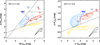 |
Fig. 1. Redshift ranges for an efficient use of the BzK and rJK colour diagrams. Left:BzK diagram for the selection of 0.3 ≤ z < 1.0 QGs. The yellow, blue, and red contours represent the loci of stars, SFGs, and QGs at 0.3 ≤ z < 1.0 selected by the NUVrJ + BzK selection. Sources with a 3σ detection at 24 μm in Jin et al. (2018) have been excluded. The black lines represent the original cuts by Daddi et al. (2004) to select galaxies at 1.4 ≲ z ≲ 2.5. The red lines show our cut at low redshifts (Eq. (1)). For reference, the tracks show the synthetic colours for the 13 Gyr elliptical (E), early-type spirals (Sa), and M82-like templates by Polletta et al. (2007), as marked in the labels. The colours are computed for 0.3 < z < 1.5 in step of Δz = 0.3. No evolutionary effects are included. The black segments show the reddening vectors at z = 0.3, 1, and 2. Right:rJK diagram for the selection of 1.0 ≤ z < 1.4 QGs. The yellow, blue, and red contours represent the loci of stars, SFGs, and QGs at 1.0 ≤ z < 1.4 selected by the NUVrJ + rJK selection. The remaining lines are coded as in the left panel. |
The addition of the BzK and rJK criteria removes more efficiently the red dusty galaxies contaminating the sample of quiescent objects selected with the NUVrJ diagram only. Sources without a constraint on the observed colours occupy regions of the NUVrJ diagram with bluer r – J and redder NUV-r colours, partially overlapping with the final quiescent sample only below z < 1. On the other hand, galaxies excluded by the BzK and rJK criteria lie close to the line separating the star-forming population. A 2D Kolmogorov-Smirnov test (Fasano & Franceschini 1987) suggests that both the unconstrained and excluded galaxies are drawn from a parent distribution different from the one of the final quiescent sample.
The validity of the double-colour selection is further supported by the lower fraction of Spitzer/MIPS 24 μm 3σ detected red galaxies when using NUVrJ + BzK and NUVrJ + rJK colour selections (∼15%), rather than a simple NUVrJ diagram (∼25%). For the comparison we use the latest 24 μm catalogue by Jin et al. (2018), reaching an rms of ∼15 μJy. Figure 2 shows that we can trace SFRs down to several times below the MS parameterised as in Schreiber et al. (2015). To compute the SFR limit in Jin et al. (2018), we rescaled the redshift-dependent, MS templates by Magdis et al. (2012) to match the observed 24 μm depth and then integrated over the wavelength range 8 − 1000 μm to derive the total infrared luminosity (LIR). We smoothed over the width of the Spitzer/MIPS 24 μm filter to avoid the strong impact of the PAH features.
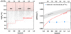 |
Fig. 2. Selection and binning. Left: grey points showing the final sample of double-colour selected and 24 μm faint QGs in the redshift vs. stellar mass plane. The rose area and the black grid mark the limits of the bins used to group galaxies for stacking. The number of stacked sources per bin are displayed. The red line indicates the 90% stellar mass completeness limit for QGs in the ‘deep’ UltraVISTA sample (Laigle et al. 2016), adjusted for the different IMF. Right: blue points showing the position of the stacked massive QGs (M* > 1010.8 M⊙) in the redshift vs. sSFR(UV) plane. The error bars on the redshift indicate the width of the bins. Only the statistical uncertainties on sSFR(UV) are shown on the y-axis. The solid red line indicates the 3σ detection limit for Spitzer/MIPS at 24 μm (σ = 15 μJy, Jin et al. 2018) converted to SFR using the MS templates from Magdis et al. (2012) and assuming M* = 1011.2 M⊙, matching the median stellar mass of our sample in each redshift bin. The grey shaded area and the grey line indicate the location of the MS and its 0.3 dex scatter, computed for a galaxy with M* = 1011.2 M⊙. |
We excluded all the 24 μm detected sources in the Jin et al. (2018) catalogue from our sample of QGs. We remark that the sample in the highest redshift bin could still potentially be contaminated by a fraction of galaxies closer to the MS, given the looser constraints on the IR emission. However, most of the contamination in the quiescent sample is due to dusty starbursts (or transitioning galaxies), rather than blue objects on the MS with undetectable IR emission. Indeed, absent IR detections, the median sSFR(UV) of the final stacked samples of massive quiescent objects is constant over the redshift interval under consideration. Therefore, the median location with respect to the MS decreases with redshift, given the steady increase in the normalisation of the former (Fig. 2).
For the purpose of stacking, we further excluded the 1% of the sample that lay too close to the edges of the IR image mosaics. Finally, we binned our sample by redshift, as shown in Fig. 2. We split the galaxies selected with the rJK colour at z = 0.65, the mid-point of the redshift interval over which this criterion is effective. In this work we focus on a complete sample of massive galaxies at 0.3 < z < 1.5 (log(M*/M⊙)≥10.83)2, matching the median stellar mass of similarly selected objects at ⟨z⟩ = 1.8 from G18. This allows us to consistently trace the evolution of the dust content over 10 Gyr of cosmic evolution. We report the properties of the stacked sample in Table 1.
Physical properties of the stacked quiescent samples.
3. Source stacking and extraction
Our stacking and source extraction methodology broadly follows that described in G18, namely: For each redshift bin, we extracted cutouts, centered on each galaxy, from publicly available FIR imaging of the COSMOS field at 24 μm (Le Floc’h et al. 2009), 100 μm, and 160 μm (Lutz et al. 2011), 250 μm, 350 μm, and 500 μm (Oliver et al. 2012), 850 μm (Geach et al. 2017), 1.1 mm (Aretxaga et al. 2011), 10 cm (Smolčić et al. 2017), and 20 cm (Schinnerer et al. 2010). For each band, we then combined the cutouts to create a median image, ignoring masked (e.g., zero-coverage) regions, and estimated the variance of each pixel through bootstrap resampling of the data with half the sample size. We note that these variance cutouts do not show any appreciable structure (i.e. they are flat), suggesting that there is little to no contribution from clustering to the noise (e.g., Béthermin et al. 2012).
As in G18, we model the emission in each median image with a combination of three components: point-like emission from the central QG, an autocorrelation term due to source overlap within the sample, and extended emission from SFGs associated with the central QGs. This includes both true SF satellites of the QGs and the two-halo term arising from clustering with more massive SFGs. For simplicity, we hereafter refer to it as the ‘satellite halo’. Finally, we also include a flat background term. As the point-source and autocorrelation terms arise from the same galaxy population their amplitudes are tied and we determine their relative scaling beforehand. To model the combined central point-like emission and autocorrelation signal, we first created simulated images of the COSMOS field for each redshift bin, consisting of a blank map populated by model or empirical beams (depending on the data) located at the position of each QG and normalised to the same unitary flux. This latter approximation was used because the scatter of the FIR flux of our QGs is unknown by construction of the sample. Consequently, we do not associate an uncertainty with the shape of the autocorrelation signal. The simulated sources were then extracted using the same procedure as described above. This yields median cutouts that are essentially indistinguishable from point-sources in the case of higher-resolution data (e.g., at 24 μm) but deviate substantially from it when the beam is large, due to the blending of sources. In particular, the SPIRE (250 μm, 350 μm, and 500 μm) ‘point’ stacks have therefore extended wing-like emission and higher peak values than a simple beam, while the 850 μm and 1.1 mm point stacks show an opposite effect, with lower peak values, arising from the deep negative rings in their PSFs. This additional step, which accounts for the intrinsic clustering of QGs, is necessary here since we did not eliminate projected pairs during selection, as in G18. Indeed, excluding from the sample all objects that partially overlap in the lowest-resolution maps (SPIRE) would more than halve it3.
On the other hand, the distribution of FIR emission from satellite halos is estimated using multi-wavelength catalogs available for the COSMOS field (Muzzin et al. 2013b; Laigle et al. 2016). Satellites were selected in the catalogue as objects that both satisfy the UVJ criterion (Williams et al. 2009) for SFGs and have compatible photometric redshifts, namely zL68 < zcen < zH68, where zcen is the redshift of the central QG and z*68 are the lower and upper 68% confidence limits to the redshift of satellites, respectively. We estimated the SFR of each satellite candidate by fitting its rest-frame ultraviolet SED with constant star formation history stellar population templates (Bruzual & Charlot 2003), with and without dust extinction. The difference between these two estimates yields an obscured SFR surface density that, when convolved with the instrumental beam in each band, is assumed to be proportional to the FIR flux distribution from the satellite halo. More details are given in Appendix A.
To extract the FIR SED of the QGs in each redshift bin, we fitted the cutouts in each band with combinations of these two components plus a flat background term. We let the scaling of the satellite emission vary freely at 24 μm, 100 μm, and 160 μm, where the resolution is high enough to properly decompose the observed signal into point-like and extended components.
Satellite fluxes in these three bands were then fitted with a set of redshift-dependent MS IR templates (Magdis et al. 2012) that capture the average value and the scatter of Td and ⟨U⟩ of MS galaxies at a given redshift (e.g., Magdis et al. 2012; Béthermin et al. 2015). From these templates (and their scatter) we extrapolated satellite fluxes (and their uncertainties) at ≥250 μm, where both the point-like and halo emission are extended and the large beams preclude a non-degenerate decomposition. For these bands, the scaling of the satellite model was fixed to the extrapolated flux, with only the background and central source being fitted. The satellite fluxes thus removed from the FIR SED correspond to log(LIR/L⊙) = 10.40 ± 0.09, 10.70 ± 0.07, and 9.30 ± 0.10 for the high-, intermediate-, and low-redshift bins, respectively. These estimates are consistent with the predicted LIR infrared from the obscured SFR of the satellites as inferred by the UV/optical modelling (log(LIR/L⊙) = 10.47 ± 0.13, 10.77 ± 0.09, and 9.70 ± 0.38). Finally, we note that while these LIR values are comparable to or higher than the LIR of QGs, the sum of the autocorrelation and the QG component still dominates the ≳250 μm bands due to a combination of lower Td and large autocorrelation term.
The fits of the various components were done with pixel weights derived from the stacked variance maps described at the beginning of this section. However, these cannot be used to estimate accurate uncertainties on the extracted fluxes as the pixel-to-pixel variance is necessarily correlated in the FIR due to confusion. Therefore, rather than considering the (small) formal errors on scaling of the combined point-source and autocorrelation models, uncertainties on central fluxes were estimated by fitting instrumental beams at random positions in the cutouts, well clear of both the central source and satellite emission. To these we added in quadrature the error of both the satellite fluxes and background, in the corresponding band. We note that the autocorrelation term alone is free of uncertainty by construction, the sample being set and the beam models in ≥250 μm bands (where it is not negligible) being theoretical and provided without associated errors. The uncertainties for each decomposition component are presented in Table A.1.
Finally, the measured central QG fluxes were rescaled down to account for contamination due to random clustering in the image using the corrections described in Béthermin et al. (2015). We note that the background term might not necessarily be flat, due to lensing from the QGs’ host dark matter halo. Magnification bias is typically dominated by area increase, so its net result is a deficit in faint source counts with respect to the field. Assuming that the QGs are central to their halo, this should lead to a lower effective background towards the centre of the cutouts, thus slightly underestimated central fluxes. However, its magnitude depends on the shape of the luminosity distribution of background sources, for which we have little to no information. Furthermore, this effect can be mild even for massive galaxy clusters (e.g., Umetsu et al. 2014). In this case, where the host halos are smaller by a factor of ∼10 (G18), we do not expect it to be significant. The final photometry of our stacked QGs is presented in Table 2 while the various decomposition components for each redshift bin and each broadband photometry are presented in Appendix A.
Stacked photometry of the QG population, as derived through flux density decomposition.
4. SED modelling
To derive the FIR properties of the stacked samples, we employed the dust models of Draine & Li (2007; DL07), with the standard parameterisation used in previous studies (e.g., Magdis et al. 2012). Namely, we considered diffuse ISM models with radiation field intensities ranging from 0.1 ≤ Umin ≤ 50, while fixing the maximum radiation field to Umax = 106. We allowed for γ (the fraction of dust exposed to starlight with intensities ranging from Umin to Umax) to vary between 0 ≤ γ ≤ 0.5 with a step of 0.01 and adopted Milky Way dust models with qPAH (i.e. the fraction of the dust mass in the form of PAH grains) from 0.4% to 4.6%. To account for the artificial SED broadening due to the redshift distribution of the stacked sources, we constructed an average SED for each DL07 model by co-adding each original DL07 model at each redshift within the bin, weighted by the redshift distribution of stacked sources. The redshift-weighted, ‘smoothed’ models were shifted to the median redshift of each bin and were fit to the data, yielding best-fit LIR, Mdust, and ⟨U⟩ values.
To estimate the uncertainties of the derived parameters we bootstrapped and fitted with same methodology 1000 artificial realisations of the real SEDs, by perturbing the extracted photometry within 1σ for the detections (S/N ≥ 3) and within flux +3σ for the rest, following the methodology presented in Béthermin et al. (2020). As uncertainty for each derived parameter from the real data, we adopted the standard deviation of the values of the corresponding parameter inferred from the perturbed SEDs. As a sanity check we also introduced a bootstrapping component in our analysis by randomly excluding one observed data point at each realisation. We also confirm that the data sets of available detections (which include at least one data point at λrest ≥ 220 μm for all four stacked ensembles, as well as a detection at 24 μm and at least one detection in the Wien part of the SED), along with the upper limits, ensure against possible systematic effects in the derivation of Mdust and LIR for all redshift bins (see Appendix D). Finally, to derive ‘luminosity-weighted’ Td we complemented our analysis by considering a single-temperature optically thin modified blackbody (MBB) models with a fixed effective dust emissivity index of β = 1.8.
The best fit models to the data (24 μm to 1.1 mm for DL07 and λrest> 50 μm to 1.1 mm for MBB), along with the range of SEDs from the random realisations, are shown in Fig. 3. The best fit parameters and their corresponding uncertainties are summarised in Table 1. While the radio data points are not included in the fit, we add to each the best-fit DL07 model a power-law radio slope with a spectral index α = 0.8 and a normalisation given by the FIR–radio correlation (e.g., Delhaize et al. 2017), to investigate (and visualise) possible radio excess in our stacked ensembles.
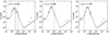 |
Fig. 3. Observed median IR SEDs of massive QGs. The magenta circles mark the observed photometry, with arrows indicating 3σ upper limits for bands where the measured flux density was negative. We note that the radio points at 10 and 20 cm were not included in the modelling. The black line and the grey shaded areas indicate the best-fit model from the Draine & Li (2007) templates and the associated uncertainty. The dashed orange line is the best fit adopting a single Td modified black body. The left, middle, and right panels show the results for the redshift intervals 0.3 < z < 0.65, 0.65 < z < 1.0, and 1.0 < z < 1.4, respectively. Salient properties of the sample are reported in Table 1. |
5. Results
Using the derived parameters from the SED modelling in the previous section, we attempted to characterise the dust and gas content of QGs and investigate possible evolutionary trends. For the rest of the analysis we will be referring to the ⟨z⟩ = 0.50, 0.85, and 1.20 stacks as low-z, mid-z, and high-z quiescent sample respectively. We also complemented our study with the stacked ensemble of G18 at ⟨z⟩ = 1.75, which has been constructed and analysed using similar sample selection, stacking, photometry, and SED modelling techniques as those adopted here. Overall, this work covers the average properties of QGs in the redshift range 0.3 < z < 2.0 with a homogeneous and systematic approach.
5.1. Basic FIR properties
The available mid-IR to millimetre photometry that spans from observed 24- to 1100 μm allows for a robust determination of the total 8–1000 μm infrared luminosities (LIR), dust masses (Mdust), mean radiation field (equivalent of dust mass-weighted luminosity or temperature), parametrised as ⟨U⟩ ∝ Mdust/LIR, and luminosity-weighted dust temperatures (Td). Our SED fitting yields low infrared outputs for our stacked ensembles at all redshifts with log(LIR/L⊙) = 9.40 − 10.30, dust masses in the range of log(Mdust/M⊙) = 7.50 − 8.15, low mean radiation field ⟨U⟩ = 0.6 − 1.2, and cold Td < 23 K dust temperatures.
In comparison to previous studies that presented stacked SEDs of QGs at similar redshifts and equivalent M* bins, our analysis yields significantly lower LIR and Mdust estimates. For example, fitting the photometry presented in Man et al. (2016) with same methodology as for our data, we find log(LIR/L⊙) = 9.8 − 11.2 and log(Mdust/M⊙) = 8.0 − 8.6 for the stacked ensembles of QGs at z = 0.4 − 1.6. These values are 0.2 − 0.9 dex larger than the corresponding parameters inferred from our analysis for our sample. These discrepancies stem from the more conservative sample selection that we adopted in this work (double-colour criterion and exclusion of individually detected 24 μm sources). In addition, the adopted stacking and, especially, the treatment and correction for the contribution of blended satellites further affects the comparison with Man et al. (2016, see also G18). Nevertheless, and in agreement with Man et al. (2016), we do find a radio excess between the observed radio fluxes and those inferred by the infrared-radio correlation of SFGs by Delhaize et al. (2017), indicative of AGN activity and ‘radio-mode’ feedback in massive QGs (e.g., Gobat et al. 2018; Barišić et al. 2017).
In order to test for the possible sensitivity of these recovered parameters to the selection criteria described in Sect. 2, as well as possible contamination of quiescent samples by dusty star forming objects, we performed a series of tests using sub-samples obtained by either applying an additional 0.1 mag colour margin or by dividing the low-, mid-, and high-z bins into blue and red halves. Applying the same stacking, source extraction, and modelling procedures, as described in Sects. 3 and 4, to these yields SEDs that are entirely consistent with the full low-, mid-, and high-z samples. This suggests that our analysis is robust with respect to selection effects. More details are given in Appendix B.
Finally, we inferred gas masses (Mgas) estimates by converting the derived Mdust to Mgas through the metallicity-dependent dust to gas mass ratio (GDR) equation of Magdis et al. (2012); log(GDR) = 10.54 − 0.99 × (12 + log(O/H)). We considered a range of metallicities Z⊙ ≤ Z ≤ 2 Z⊙ (8.66 ≤ 12 + log(O/H) ≤ 9.1 in the Pettini & Pagel 2004 scale), appropriate for the SFR and M* of our samples (e.g., Mannucci et al. 2010). For these metallicities the GDR varies between 35≤ Mgas/Mdust ≤ 92. For the rest of our analysis we use the Mgas estimates based on a solar metallicity as benchmark and those for a super-solar metallicity as lower limits. Therefore, throughout the paper, Mgas =  (and fgas =
  ), unless otherwise stated. We note that since the Mdust/Mgas − Z relation of Magdis et al. (2012) is almost linear (slope of 0.99), we can easily rescale Mgas estimates between solar and an arbitrary metallicity Y by using:
![$$ \begin{aligned} \mathrm{log} [M^{Y}_{\rm gas}] = \mathrm{log} [M^\mathrm{sol}_{\rm gas}] + [8.66 - Y],\,\,\,\, Y = 12 + \mathrm{log(O/H)} . \end{aligned} $$](/articles/aa/full_html/2021/03/aa39280-20/aa39280-20-eq19.gif)
We also recall that the GDR – Z relation yields Mgas estimates that trace the sum of the atomic (MHI) and the molecular (MH2) gas mass (including a ×1.36 He contribution). As such, Mgas = MHI + MH2. While the exact state of the cold gas in our QGs cannot be characterised, the ⟨MH2/MHI⟩> 1 ratios reported in the literature for z > 0.5 and for high stellar surface densities (e.g., Blitz & Rosolowsky 2006; Bigiel et al. 2008; Obreschkow et al. 2009) motivate us to make the simplified assumption that MH2 ≫ MHI and, thus, MH2≈ Mgas. We note though, that this estimate is an upper limit to the molecular gas mass of our samples.
5.2. Evolution of dust and gas mass fractions
In Fig. 4 we bring together the Mdust estimates for our stacked ensembles as well as a range of literature Mdust estimates for local QGs of comparable M* (Smith et al. 2012; Boselli et al. 2014; Lianou et al. 2016; Michałowski et al. 2019) and explore the evolution of dust mass fraction, Mdust/M*, as a function of redshift. Our data indicate that the Mdust/M* remains roughly constant from z = 2.0 to z = 1.0, followed by sharp decline towards the present day, with a functional form of Mdust/ (for z < 1.0). As shown in Fig. 4, a similar trend characterises the evolution of the dust mass fraction in SFGs Kokorev et al. (2021), albeit with a shallower slope. Evidently, QGs exhibit systematically lower dust mass fractions with respect to SFGs at all redshifts, indicative of dust consumption, destruction or expulsion during the quenching phase. However, the flat evolution for QGs between z = 2.0 − 1.0 and the monotonically decreasing Mdust/M* for SFGs at all redshift, results in a minimum deviation between the two populations at z ∼ 1.0.
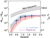 |
Fig. 4. Evolution of the dust to stellar mass ratio and of the gas fraction of QGs. The filled blue circles mark the Mdust/M* of the stacked QGs in the 0.3 < z < 2.0 range, including the results from G18. The grey shaded region depicts the trend for MS galaxies from Kokorev et al. (2021). The orange shaded region captures the range of Mdust/M* for local QGs, as drawn from the literature (see text). The dotted blue line (blue shaded region) corresponds to the best fit (scatter) to the 0.0 < z < 1.0 Mdust/M* data of QGs, with a functional form of Mdust/M* ∝ (1 + z)5.0. The bold, dashed purple line (shaded region) depicts the evolution (scatter) of Mdust/M* (and of fgas) as derived from the progenitor bias analysis of Gobat et al. (2020), which is discussed in Sects. 5.2 and 6. The conversion of Mdust/M* to fgas assumes solar metallicity and GDR = 92. |
The evolution of Mdust/M* we find here also mirrors the evolution of the gas fraction of QGs. Under the assumption of constant solar metallicity for massive QGs at all redshifts, we can directly convert the Mdust/M* presented in the left y-axis of Fig. 4 to fgas. This approach yields a constant fgas ≈ 7 − 8% between z = 2.0 − 1.0 that subsequently drops to fgas ≈ 2% at z = 0.5 and fgas ≤ 1% in the local Universe. These values are in agreement with independent Mgas estimates or upper limits inferred by CO observations of individual QGs and post-starburst galaxies at various redshifts (e.g., French et al. 2015; Sargent et al. 2015; Rudnick et al. 2017; Suess et al. 2017; Spilker et al. 2018; Bezanson et al. 2019). We note that for a super solar metallicity of 2 × Z⊙ the fgas values presented in Fig. 4 would correspond to  . In Sect. 6, we will interpret the observed redshift evolution of Mdust/M* and fgas of QGs in terms of progenitor bias and ageing of the stellar population.
5.3. SFR and gas depletion time scales
The gas masses inferred in the previous section, when coupled with the corresponding SFRs of the stacked ensembles, can be used to define the star formation efficiency (SFE = SFR/Mgas) or, inversely, the gas depletion time scale (τdep = 1/SFE). To derive the total SFR in each redshift bin, we considered the average unobscured component as derived from the optical photometry (SFRUV) and the obscured star formation by converting LIR to SFRIR using the Kennicutt (1998) scaling relation. We caution the reader that for QGs a considerable fraction of LIR could arise from dust heated by old rather than young stellar populations (e.g., Hayward et al. 2014), as assumed by the Kennicutt SFR-LIR relation. Therefore, the estimates of SFRtot = SFRIR + SFRUV should be regarded as upper limits. To constrain the fraction of LIR arising from dust heated by old stars, we fit each galaxy’s optical-NIR SED with composite stellar population models derived from Bruzual & Charlot (2003) templates. For simplicity, we used delayed exponential star formation histories, starting at zin = 10 and with time scales τ = 100 Myr−3 Gyr, each truncated 1 Gyr before observation. Finally, we assumed a Noll et al. (2009) attenuation curve with variable slope and computed the luminosity difference of the best-fit model before and after attenuation. We find that this absorbed energy does not make up more than ∼30% of LIR at z ≳ 1 but could represent up to 100% of the infrared luminosity of z ∼ 0.5 QGs. Given the uncertainties and the small IR output indicated by our stacks, we chose to consistently consider SFRtot at all redshift bins.
The emerging (maximum) SFRs are listed in Table 1 and they range from ∼2.0 M⊙ yr−1 in the lowest redshift bin (⟨z⟩ = 0.5) to ∼6.5 M⊙ yr−1 at ⟨z⟩ = 1.8. These average SFRs place our stacked ensembles ≥10× below the MS at their corresponding redshifts, confirming their passive nature. At the same time, τdep, ranges from 1.3 to 3.0 Gyr for the case of solar metallicity with a mean ⟨τdep ⟩ = 2.1 ± 0.8 Gyr and 0.5–1.1 Gyr for a super solar metallicity. These τdep estimates are plotted as a function of SFR and redshift in the two panels of Fig. 5 along with the corresponding tracks for MS galaxies (Sargent et al. 2014; Liu et al. 2019). We stress again that since we are using the maximum SFR estimates the quoted τdep should be regarded as lower limits for each metallicity. In agreement with Spilker et al. (2018), we find that distant QGs, for their SFRs, have a τdep that is broadly consistent with that of local MS galaxies, but longer than that of MS galaxies at their corresponding redshift. We note that while our data hint upon an increase in τdep from z = 2.0 to z = 0.8 followed by a decline towards later cosmic epochs (Fig. 5, right), the values are overlapping within their uncertainties yielding a non significant correlation. Possible metallicity effects as well as the uncertainties linked to the conversion of LIR to SFR, will be investigated in detail in a future study.
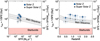 |
Fig. 5. Gas depletion timescales. Left: gas depletion time scale (tdep) as a function of SFR. The blue (grey) circles correspond to the stacked samples of QGs for the case of solar (super solar) metallicity, assuming GDR = 92 (35). The dashed grey line and the grey shaded region depict the trend for MS galaxies from Sargent et al. (2014) with a scatter of 0.23 dex. The magenta shaded region marks the area with τdep < 100 Myr, typical of star-bursting galaxies. Right: gas depletion time scale as a function of redshift. The symbols are the same as in the left panel. The dashed grey line and the grey shaded region depict the trend of Liu et al. (2019) for MS galaxies at fixed M* = 2 × 10¹¹ M⊙ and its corresponding scatter of 0.23 dex. |
5.4. SED and Td evolution
The star formation activity and the dust heating photons per unit ISM mass, both parametrised above in terms of SFR, Mdust, and SFE, should also be imprinted in the shape of the FIR SED and the characteristic Td of QGs. Indeed, a large body of literature that has focused on the evolution of Td as a function of redshift for MS and star-bursting galaxies alike (e.g., Hwang et al. 2010; Magdis et al. 2012, 2017; Magnelli et al. 2014; Schreiber et al. 2018a; Jin et al. 2019; Cortzen et al. 2020) has established that the increase in sSFR and SFE at higher redshifts is also followed by a trend of warmer SEDs and increasing Td at least out to z ∼ 4. At the same time, SEDs and the effective Td of distant QGs as a function of redshift are far less explored.
In Fig. 6 we plot the Td of QGs derived from our MBB fits as a function of redshift, along with literature data and trends for MS galaxies. As expected, QGs exhibit colder Td with respect to star forming galaxies at all redshifts, indicative of a lower star formation activity. Also, at first reading, the Td estimates for our quiescent ensembles are overlapping within their uncertainties, with an average ⟨Td⟩ = 21.0 ± 2.0 K. Notably, in the redshift range probed by our data, SFGs have witnessed a decrease in their Td by ∼8 K, indicative of a steep evolution that is not observed for QGs.
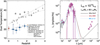 |
Fig. 6. Dust temperatures and average SED. Left: the evolution of Td in QGs. The filled blue circles mark the luminosity-weighted Td for the stacked QGs at 0.3 < z < 2.0, including the results from G18. Filled grey triangles and squares indicate SFGs on the MS and strong starbursts from Béthermin et al. (2015). Filled and open grey circles represent the mass-averaged values and the most massive galaxies (11.0 < log(M*/M⊙) < 11.5, Salpeter IMF) for the star-forming sample of Schreiber et al. (2018a), respectively. The solid and dashed grey lines indicate the best fit models from Schreiber et al. (2018a) and Béthermin et al. (2015), extending the parameterisation of Magdis et al. (2012). The dotted grey line indicates the expected Td track for a size evolution of QGs, R ∝ (1 + z)−1.48. The track is normalised to the Td of the z = 1.8 sample. Right: composite and template FIR SED for z > 0 QGs. The magenta circles (arrows) correspond to the photometry (3σ upper limits) of the stacked ensembles presented in Fig. 3 normalised to LIR = 1010 L⊙ (and Mdust = 1.11 × 10⁸ M⊙). The DL07 and MBB model fits to the SED are shown with grey and red dashed lines. The dotted blue line correspond to the typical SED of z = 1.0 MS galaxies from Magdis et al. (2012), normalised to the same LIR. The QG template is publicly available at www.georgiosmagdis.com/software/. |
However, the hint of small Td decrease in QGs between z = 2.0 and z = 0.3 (ΔTd ≈ 3 K), even if not statistically vigorous, provides the grounds for a tempting speculation of a weak evolution driven by their size evolution. Indeed, a size evolution of R ∝ (1 + z)−1.48 (van der Wel et al. 2014) yields a size increase of a factor of ∼0.5 between z = 1.8 and 0.8. Similarly, following the analysis of Chanial et al. (2007),  ∝ [ΣIR]γ, where
  and ΣIR ∝ LIR/R2. For fixed LIR (or SFR), as in the case for our stacked samples in this redshift range, it follows that Td(z1)/Td(z2) ∝[R(z2)/R(z1)]2 × γ/(4 + β). Anchoring this equation at Td(z = 1.8) = 23.5 K, as inferred by our analysis and adopting β = 1.8, provides an evolutionary track that is in broad agreement with our measurements for the 0.3 < z < 2.0 stacks. We conclude that a weak (if any) evolution of Td in QGs can be understood in terms of size growth. At the same time an average ⟨Td⟩ = 21.0 ± 2.0 K provides a statistically robust estimate for a characteristic Td for the ISM of QGs over the last ten billion years.
In addition, the small variance in Td and LIR/Mdust, suggests that massive QGs at various redshifts share a common FIR SED shape, albeit with a varying normalisation that mirrors the evolution of LIR and of the ISM mass budget as described in the previous sections. To produce an average SED, we bring the stacked photometry of each redshift bin at rest-frame, normalise it so that all SEDs are anchored at the same reference luminosity of 1.0 × 10¹⁰ L⊙, and fit with DL07 and MBB models following the methodology presented in Sect. 4. The observed points (and upper limits) along with the best-fit models are presented Fig. 6 (right). The emerging average SED of QGs has Td = 20 K, and LIR/Mdust ≈90 L⊙/M⊙, in direct contrast to that of typical z > 0 star forming galaxies. As an example, we consider the average SED of z = 1.0 MS galaxies from Magdis et al. (2012), which clearly peaks at shorter λ with a Td ≈ 30 K and has approximately a factor of ∼10× larger infrared energy output per unit dust mass (LIR/Mdust ≈ 1000 L⊙/M⊙). Finally, we stress that the radio data are not included in the fit but are presented to demonstrate the radio-excess that we have already briefly discussed in a previous section. The average SED of QGs (normalised to LIR = 1.0 × 10¹⁰ L⊙ and Mdust = 1.11 × 10⁸ M⊙) is publicly available4.
6. Discussion
In the previous sections, we characterised the mass budget and the properties of the ISM of QGs at various redshifts. Here we offer an explanation for the origin and the drivers of the observed trends.
To interpret the evolution of Mdust in our quiescent sample, we first need to consider the expected redshift evolution of a population of QGs. At log(M*/M⊙)∼11.0, their co-moving number density increases significantly between z ∼ 4 and z ∼ 1, with little evolution after that (e.g., Muzzin et al. 2013a; Davidzon et al. 2017). This implies that an unbiased sample of QGs will contain a large fraction of newly formed objects at any redshift z ≳ 1 while, few new objects enter the z < 1 population. For simplicity, let us neglect dry merging events and equate the formation time of a QG with the quenching time of its precursor. In this case, the average age of the quenching event will vary little between quiescent galaxy samples at z ≳ 1 and increase with cosmic time at z ≲ 1. In this context, the apparent non-evolution of the dust fraction between z ∼ 2 and z ∼ 1, where newly quenched galaxies constitute a large part of the quiescent population, suggests that whatever quenching mechanisms are at play, they leave behind very similar ISM conditions independently of redshift. Conversely, the steep decrease in the dust fraction between z ∼ 1 and z = 0 is consistent with a consumption (or destruction) without replenishment of the dust and gas as few to no new QGs enter the massive population in this redshift range. Combining both regimes yields an apparent evolution very similar to our observed constraints, as shown in Fig. 4. Here we estimated the median gas fraction of the whole population of QGs as a function of redshift by assuming only the QG production rate from stellar mass functions, an initial gas fraction (constant with redshift) of ∼10% immediately following quenching, and a closed-box consumption with a time scale of ∼2 Gyr after that (Gobat et al. 2020). The track derived in this manner reproduces our data well, especially when considering that the latter are likely slightly biased towards dustier objects at lower redshift (see Fig. 2), which would flatten the observed trend.
This ‘progenitor-bias’ explanation for the observed evolution of fgas and Mdust/M* would also require an anti-correlation between these quantities and the average quenching time, or more simply, the stellar age. Indeed, in a recent study, Michałowski et al. (2019), presented an exponential decline of the Mdust/M* with age for a sample of galaxies at a fixed cosmic epoch (⟨z⟩ = 0.13) and a range of luminosity-weighted stellar ages between 9.0 < log(age/yr) < 10. The authors report a decline of Mdust/M* with age that follows e−age/τ and a dust lifetime τ≈ 2.5 Gyr. While we do not have any information about the actual stellar age of the galaxies in our stacks, the effect of varying age can be mimicked by the our different redshift bins and under the assumption that the passive galaxies at z > 0.9 will, on average, remain passive at later times. Indeed the time interval between z = 0.9 and z = 0.5 corresponds to ≈2.3 Gyr. According to the formula of Michałowski et al. (2019), and assuming an average stellar age of 2 − 3 Gyr for the QGs at z = 0.9, we should expect a drop in log(Mdust/M*) by ∼0.4 − 0.6 dex, in very good agreement with our observations. At the same time, as described above, the flat behaviour of the Mdust/M* (and fgas) at z > 1.0 could then be explained by the younger, and roughly constant stellar age of the QGs in the higher redshift bins (e.g., log[Age/yr] = 9.0 at z = 2.0 − 4.0, Toft et al. (2017), Valentino et al. (2020)).
Finally, the rather constant FIR SED shape (and Td) of QGs at all redshifts, indicate that LIR and Mdust roughly scale together irrespective of the time of quenching. If indeed LIR is a proxy of SFR and Mdust a proxy of Mgas this means that the decrease in Mgas is closely followed by a decrease in SFR. In this case, the universality of the initial ISM conditions, as advocated by the evolution of ISM mass budget (in terms of fgas and Mdust/M*), is followed by a regularity in the internal processes within quenched galaxies.
We should stress that while the progenitor bias offers an appealing empirical explanation for the observed evolution of the ISM properties of QGs, it bares little, if any, information about the underlying physics of the origin and the maintenance of quenching. For the latter, the radio excess present in our SEDs as well as in previous studies (e.g., Man et al. 2016; D’Eugenio et al. 2020), point towards ‘radio-mode’ feedback from AGN-driven jets as compelling quenching mechanism that can both prevent gas accretion due to heating of the halo gas and expel a fraction of the cold gas reservoir (e.g., Croton et al. 2006; Gobat et al. 2018). This radio-mode feedback would also need to be stronger at higher redshift to compensate for the higher (putative) gas fractions seen at these epochs. Using the average 1.4 GHz excess, with respect to the FIR-radio correlation, and the evolution of the AGN luminosity function (Novak et al. 2018), we indeed estimate that the AGN duty cycle for our QGs decreases from > 50% at z ∼ 1.8 (see G18) to ∼15% in the low-z redshift bin (see Appendix C).
6.1. Outlook and ALMA predictions
From the discussion above, it stems that the Mdust (and subsequently Mgas and fgas) of QGs depends both on redshift and on time elapsed since the quenching event. So while our Mdust and Mgas estimates should be valid for the average QGs population at a given redshift, this might not be the case for individual sources due to possible age variations. Clearly, the way forwards necessitates focused ISM studies for large and representative samples of individual QGs at various cosmic epochs. In this regard, the IR SED template presented in Sect. 5, can facilitate a series of useful predictions.
The main characteristic of the template is the ratio of its native infrared luminosity ( ) to its native dust mass (
 ), which is expressed as
  /
/ /M⊙. Consequently, for any arbitrary normalisation of the template, it follows that for this template, LIR = 90 × Mdust [in L⊙]. Similarly, Mgas, for a fixed metallicity Z, scales linearly with Mdust, with Mgas = GDR(Z) × Mdust (e.g., Leroy et al. 2011; Magdis et al. 2012). Therefore, the template can be rescaled to any arbitrary Mdust that corresponds to a given Mgas (or fgas). Indeed, since fgas = Mgas/M* = GDR(Z) × Mdust/M* we simply have to multiply the SED by N = Mdust/
 , which takes the form of:
Assuming that our SED is representative of massive QGs with a typical log(M*/M⊙) = 11.2 at all redshifts and by adopting a universal solar metallicity that corresponds to GDR(Z⊙) = 92 (e.g., Leroy et al. 2011; Magdis et al. 2012), the only free parameter in the SED normalisation is fgas. Then we can use our normalised template SED to calculate the emitted flux density at the central wavelength of various ALMA bands at various redshifts for any adopted fgas after implementing CMB effects as prescribed in daCunha et al. (2013).
As an example, we examine the case where fgas is evolving with redshift as fgas ∝ (1 + z)5.0 at z < 1.0 and then remains flat with fgas = 8% at z ≥ 1.0 (Sect. 5). The flux density tracks as a function of redshift for various ALMA bands are presented in Fig. 7(left). We stress that these tracks are specifically tailored around massive (log(M*/M⊙) = 11.20) QGs with a solar metallicity. However, the recipe described above is also valid for any arbitrary gas phase metallicity and any M* provided that our template is also representative of less (or more) massive QGs.
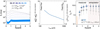 |
Fig. 7. ALMA outlook and systematics. Left: ALMA flux densities in various bands for an evolving fgas as (1 + z)5.0 at 0.0 < z < 1.0 and fixed fgas = 8%, at z > 1.0. The predicted fluxes are derived using the average DL07 SED presented in Fig. 6(right) and are corrected for CMB effects. The blue shaded region depicts the range of predicted flux densities in ALMA Band 3 assuming a 50% uncertainty in the adopted fgas. Middle: ratio of Mgas estimates, as inferred for a fixed monochromatic luminosity at a given rest-frame wavelength from (1) scaling the average SED of QGs presented in Fig. 6(right), |


We emphasise that the conversion of R-J flux densities (fALMA) to Mgas, and vice versa, is heavily dependent on the adopted method (and template). Indeed, at fixed fALMA, the commonly adopted monochromatic prescription of Scoville et al. (2017) yields systematically lower Mgas estimates with respect to those inferred in here. As shown in Fig. 7(middle) the tension between the two methods becomes more prominent at λrest closer to the peak of the SED and progressively eases moving further into the R-J tail. This is also demonstrated in Fig. 7(right) where we show how applying the Scoville et al. (2017) method at λobs = 850μm would affect the recovered evolution of fgas. We note that while we lack observations at z > 2.0 we extrapolate to higher redshifts under the assumption of flat fgas evolution at z > 2 to highlight how discrepancy (for fixed λobs) between the two methods increases at higher redshifts.
The tension in the Mgas (and fgas) estimates between the two methods, arises predominantly from the assumed Td of QGs. We recall that the Scoville et al. (2017) recipe is calibrated on SFGs, assuming a fixed ‘mass-weighted’ Td = 25 K. This corresponds to a ∼7–10 K warmer ‘luminosity-weighted’ Td compared to that of our template. Similarly, as discussed above, our QG template is ∼10 K colder with a ∼10 times lower LIR/Mdust compared to that of a typical SFG at z = 1.0. It then naturally follows that with respect to the Scoville et al. (2017) approach (or a z> 0 SFG template) our method predicts lower fALMA and subsequently a significantly longer integration time to detect dust emission from a QG of a given Mgas (e.g., ∼ × 6 for a galaxy at z = 3 and λobs = 1200 μm). This, could explain the scarce dust continuum detections among the limited number of high-z QGs that have been followed up with ALMA so far.
Another point of concern is selection biases, especially in terms of M*. Williams et al. (2021), reports no CO[2-1] detection for a sample of massive ⟨log(M*/M⊙)⟩ ≈ 11.7 (for Salpeter IMF) QGs at z ∼ 1.5, placing stringent upper limits in their fgas ≤ 1.0–3.5%, that are lower compared to our estimates. However, we note that this sample is ∼0.5–0.7dex more massive with respect to the stacked ensembles studied here. If the fgas of high-z QGs decreases as a function of M*, similarly to what is observed for SFGs and local ETGs ( e.g., Saintonge et al. 2011a; Magdis et al. 2012), then rescaling our fgas estimates accordingly would significantly ease the tension (see also Fig. 6 of Williams et al. 2021). Nevertheless, we caution the reader that (1) the dust method to infer Mgas, when applied to QGs, could in principle recover a sizeable amount of HI that is untraceable by the CO lines and (2) DL07 or similar dust emission models could be a poor representation of the dust grain composition of distant QGs.
Finally, we discuss the impact of the CMB on the predicted flux densities, an effect that was recently observationally confirmed in a sample of ‘cold’ z > 3 SFGs (Jin et al. 2019; Cortzen et al. 2020). Our analysis suggests that while fALMA should remain unaffected up to z ∼ 2.0 in all ALMA bands, the ‘dimming’ of the dust continuum emission that can be measured against the CMB is not negligable at higher redshifts and lower frequencies. This is demonstrated by the flat evolution of the flux density tracks in Bands 3–6, that clearly deviate from the expected rising trend due to the negative k-correction (Fig. 7left). Indeed, our analysis suggests that the recoverable continuum emission drops by a factor of 1.4 at z = 3–5 for Band 5 and by a factor of ∼1.6–2.0 at z = 4–5 for Band 3 observations. Admittedly, the analysis presented in this work does not extent beyond z ∼ 2, and therefore the actual IR SED (and Td) of QGs at z > 2 is still unconstrained. However, if the template SED presented here is also valid at z > 2.0, CMB-corrections should be implemented both in the observing strategy and in the interpretation of dust continuum and spectral line observations of z > 3.0 QGs in the (sub)-mm.
6.2. Caveats
As pointed out in the previous sections, this analysis is not free of caveats which are inherent to the stacking method. First, decomposing the stacked signal into various components is a challenging task. Indeed, ‘satellite’ fluxes in the SPIRE bands, and their corresponding uncertainties, depend on the adopted templates used for extrapolation. While we have considered an uncertainty on the SED of the SF component, our analysis does not account for spatially correlated variations of Tdust. This would effectively make the satellite emission term frequency-dependent. On the other hand, the average stellar mass of SFGs in the satellite halo varies, with respect to their distance to the QGs, by less than a factor of 2. This suggests that the population of SF satellites is fairly homogeneous.
Furthermore, the combined photometry in the available bands can place constraints in the shape of the SED and in the inferred FIR properties, under the assumption that the FIR emission of QGs is well-represented by the adopted DL07 models. This is of particular importance, especially since none of our stacked ensembles has a formal detection (S/N > 3) in the R-J tail (λrest > 350 μm). With these important considerations in mind we conclude that future infrared and millimetre observations of large and representative samples at ≤1 − 2″ resolution, are necessary to capture unequivocally the ISM mass budget and ISM conditions of high-z QGs.
7. Conclusions
In this work we presented a robust multi-wavelength stacking analysis of a carefully selected sample of massive QGs from the COSMOS field and in three redshift bins, ⟨z⟩= 0.5, 0.9, 1.2. We further complemented our sample with the stacking ensemble of Gobat et al. (2018), at ⟨z⟩ = 1.8, constructed following the same selection criteria as those adopted in the current study, as well as with literature data for local QGs. By modelling the stacked photometry, we drew the characteristic FIR SEDs, inferred the ISM mass budget, and explored the evolution of the FIR properties of massive QGs over the last ten billion years. Our results are summarised as follows:
-
The Mdust/M* ratio rises steeply as a function of redshift up to z ∼ 1.0 and then remains flat at least out to z = 2.0. The evolution of fgas follows (by construction) a similar trend, with a normalisation that depends on the assumed gas phase metallicity of the QGs. For solar metallicity, fgas increases from 2% to 8% between z = 0.5 and z = 1.0. The evolution of fgas in our QG samples can then be interpreted as a combination of progenitor bias at z > 1, a uniformity in ISM conditions among newly quenched galaxies, and a closed-box consumption of the ISM after quenching, with a depletion time of ∼2 Gyr.
-
The gas depletion time scales of massive QGs at all redshifts are comparable to that of local SFGs and systematically longer than that of MS galaxies at their corresponding redshifts.
-
The dust temperature of massive QGs remains roughly constant with Td = 21 ± 2 K out to z = 2.0, with only a weak (if any) evolution towards a marginally higher Td at higher redshifts, which can be explained as the consequence of the average size evolution of QGs. This motivated us to construct and make publicly available a template IR SED of massive z > 0 QGs.
-
Based on our template SED, we provide predictions for the flux densities of the continuum emission in the R-J tail of passive galaxies as a function of redshift, and highlight the need of accounting for CMB effects at z > 3. Finally, we argue that Mgas prescriptions calibrated on SFGs could lead to an overestimate of the predicted dust continuum flux density of QGs in the (sub)-mm bands and discuss the implications for ALMA observing strategies.
After accounting for progenitor bias, we are ultimately left with the picture of a weak to flat evolution of initial ISM conditions in QGs. That is, our current constraints do not require that the gas fraction of QGs immediately after quenching, nor the depletion time after that, change significantly in the 10 Gyr between z = 0 and z ∼ 2. This apparent regularity in the internal properties of QGs across most of the history of the Universe mirrors the consistency of star formation physics in MS galaxies throughout cosmic time. We conclude that this uniformity of QGs should extend to earlier z > 2.0 epochs, which so far lack strong constraints in this regard.
This corresponds to a log(M*/M⊙)≥10.6 mass cut in the original Laigle et al. (2016) catalogue, which is built assuming a Chabrier IMF.
Acknowledgments
GEM and FV acknowledge the Villum Fonden research Grant 13160 “Gas to stars, stars to dust: tracing star formation across cosmic time” and the Cosmic Dawn Center of Excellence funded by the Danish National Research Foundation under then Grant No. 140. FV acknowledges support from the Carlsberg Foundation research grant CF18-0388 “Galaxies: Rise And Death”. S. J. acknowledges financial support from the Spanish Ministry of Science, Innovation and Universities (MICIU) under AYA2017-84061-P, co-financed by FEDER (European Regional Development Funds). K.E.W. wishes to acknowledge funding from the Alfred P. Sloan Foundation.
References
- Agius, N. K., Sansom, A. E., Popescu, C. C., et al. 2013, MNRAS, 431, 1929 [Google Scholar]
- Alatalo, K., Lisenfeld, U., Lanz, L., et al. 2016, ApJ, 827, 106 [Google Scholar]
- Aretxaga, I., Wilson, G. W., Aguilar, E., et al. 2011, MNRAS, 415, 3831 [Google Scholar]
- Arnouts, S., Walcher, C. J., Le Fèvre, O., et al. 2007, A&A, 476, 137 [NASA ADS] [CrossRef] [EDP Sciences] [Google Scholar]
- Barišić, I., van der Wel, A., Bezanson, R., et al. 2017, ApJ, 847, 72 [NASA ADS] [CrossRef] [Google Scholar]
- Béthermin, M., Le Floc’h, E., Ilbert, O., et al. 2012, A&A, 542, A58 [NASA ADS] [CrossRef] [EDP Sciences] [Google Scholar]
- Béthermin, M., Daddi, E., Magdis, G., et al. 2015, A&A, 573, A113 [NASA ADS] [CrossRef] [EDP Sciences] [Google Scholar]
- Béthermin, M., Fudamoto, Y., Ginolfi, M., et al. 2020, A&A, 643, A2 [CrossRef] [EDP Sciences] [Google Scholar]
- Bezanson, R., Spilker, J., Williams, C. C., et al. 2019, ApJ, 873, L19 [Google Scholar]
- Bielby, R., Hudelot, P., McCracken, H. J., et al. 2012, A&A, 545, A23 [NASA ADS] [CrossRef] [EDP Sciences] [Google Scholar]
- Bigiel, F., Leroy, A., Walter, F., et al. 2008, AJ, 136, 2846 [Google Scholar]
- Blitz, L., & Rosolowsky, E. 2006, ApJ, 650, 933 [NASA ADS] [CrossRef] [Google Scholar]
- Boselli, A., Cortese, L., Boquien, M., et al. 2014, A&A, 564, A66 [NASA ADS] [CrossRef] [EDP Sciences] [Google Scholar]
- Bruzual, G., & Charlot, S. 2003, MNRAS, 344, 1000 [NASA ADS] [CrossRef] [Google Scholar]
- Cappellari, M., McDermid, R. M., Alatalo, K., et al. 2013, MNRAS, 432, 1862 [Google Scholar]
- Cattaneo, A., Dekel, A., Devriendt, J., Guiderdoni, B., & Blaizot, J. 2006, MNRAS, 370, 1651 [Google Scholar]
- Chanial, P., Flores, H., Guiderdoni, B., et al. 2007, A&A, 462, 81 [NASA ADS] [CrossRef] [EDP Sciences] [Google Scholar]
- Cimatti, A., Daddi, E., Renzini, A., et al. 2004, Nature, 430, 184 [Google Scholar]
- Civano, F., Marchesi, S., Comastri, A., et al. 2016, ApJ, 819, 62 [Google Scholar]
- Cortzen, I., Magdis, G. E., Valentino, F., et al. 2020, A&A, 634, L14 [EDP Sciences] [Google Scholar]
- Croton, D. J., Springel, V., White, S. D. M., et al. 2006, MNRAS, 365, 11 [NASA ADS] [CrossRef] [Google Scholar]
- daCunha, E., Groves, B., Walter, F., et al. 2013, ApJ, 766, 13 [Google Scholar]
- Daddi, E., Cimatti, A., Pozzetti, L., et al. 2000, A&A, 361, 535 [NASA ADS] [Google Scholar]
- Daddi, E., Cimatti, A., Renzini, A., et al. 2004, ApJ, 617, 746 [Google Scholar]
- Daddi, E., Renzini, A., Pirzkal, N., et al. 2005, ApJ, 626, 680 [Google Scholar]
- Daddi, E., Dickinson, M., Morrison, G., et al. 2007, ApJ, 670, 156 [Google Scholar]
- Daddi, E., Dannerbauer, H., Elbaz, D., et al. 2008, ApJ, 673, L21 [Google Scholar]
- Daddi, E., Bournaud, F., Walter, F., et al. 2010, ApJ, 713, 686 [Google Scholar]
- Davé, R., Rafieferantsoa, M. H., Thompson, R. J., & Hopkins, P. F. 2017, MNRAS, 467, 115 [NASA ADS] [Google Scholar]
- Davé, R., Crain, R. A., Stevens, A. R. H., et al. 2020, MNRAS, 497, 146 [CrossRef] [Google Scholar]
- Davidzon, I., Ilbert, O., Laigle, C., et al. 2017, A&A, 605, A70 [NASA ADS] [CrossRef] [EDP Sciences] [Google Scholar]
- Davis, T. A., Young, L. M., Crocker, A. F., et al. 2014, MNRAS, 444, 3427 [Google Scholar]
- Dekel, A., Birnboim, Y., Engel, G., et al. 2009, Nature, 457, 451 [Google Scholar]
- Delhaize, J., Smolčić, V., Delvecchio, I., et al. 2017, A&A, 602, A4 [NASA ADS] [CrossRef] [EDP Sciences] [Google Scholar]
- D’Eugenio, C., Daddi, E., Gobat, R., et al. 2020, ApJ, 892, L2 [CrossRef] [Google Scholar]
- DiMatteo, T., Springel, V., & Hernquist, L. 2005, Nature, 433, 604 [Google Scholar]
- Draine, B. T., & Li, A. 2007, ApJ, 657, 810 [Google Scholar]
- Elbaz, D., Dickinson, M., Hwang, H. S., et al. 2011, A&A, 533, A119 [NASA ADS] [CrossRef] [EDP Sciences] [Google Scholar]
- Fasano, G., & Franceschini, A. 1987, MNRAS, 225, 155 [NASA ADS] [CrossRef] [Google Scholar]
- French, K. D., Yang, Y., Zabludoff, A., et al. 2015, ApJ, 801, 1 [Google Scholar]
- Geach, J. E., Smail, I., Moran, S. M., et al. 2011, ApJ, 730, L19 [Google Scholar]
- Geach, J. E., Dunlop, J. S., Halpern, M., et al. 2017, MNRAS, 465, 1789 [Google Scholar]
- Glazebrook, K., Schreiber, C., Labbé, I., et al. 2017, Nature, 544, 71 [NASA ADS] [CrossRef] [Google Scholar]
- Gobat, R., Strazzullo, V., Daddi, E., et al. 2012, ApJ, 759, L44 [NASA ADS] [CrossRef] [Google Scholar]
- Gobat, R., Daddi, E., Magdis, G., et al. 2018, Nat. Astron., 2, 239 [Google Scholar]
- Gobat, R., Magdis, G., D’Eugenio, C., & Valentino, F. 2020, A&A, 644, L7 [Google Scholar]
- Gomez, H. L., Baes, M., Cortese, L., et al. 2010, A&A, 518, L45 [NASA ADS] [CrossRef] [EDP Sciences] [Google Scholar]
- Hayashi, M., Tadaki, K.-I., Kodama, T., et al. 2018, ApJ, 856, 118 [NASA ADS] [CrossRef] [Google Scholar]
- Hayward, C. C., Lanz, L., Ashby, M. L. N., et al. 2014, MNRAS, 445, 1598 [Google Scholar]
- Henriques, B. M. B., White, S. D. M., Thomas, P. A., et al. 2015, MNRAS, 451, 2663 [NASA ADS] [CrossRef] [Google Scholar]
- Hopkins, P. F., Somerville, R. S., Hernquist, L., et al. 2006, ApJ, 652, 864 [Google Scholar]
- Hwang, H. S., Elbaz, D., Magdis, G., et al. 2010, MNRAS, 409, 75 [Google Scholar]
- Ilbert, O., McCracken, H. J., Le Fèvre, O., et al. 2013, A&A, 556, A55 [NASA ADS] [CrossRef] [EDP Sciences] [Google Scholar]
- Jin, S., Daddi, E., Liu, D., et al. 2018, ApJ, 864, 56 [Google Scholar]
- Jin, S., Daddi, E., Magdis, G. E., et al. 2019, ApJ, 887, 144 [Google Scholar]
- Kennicutt, R. C. Jr 1998, ARA&A, 36, 189 [Google Scholar]
- Kokorev, V., Magdis, G. E., Davidzon, I., et al. 2021, ApJ, submitted [Google Scholar]
- Kriek, M., van Dokkum, P. G., Franx, M., et al. 2006, ApJ, 649, L71 [Google Scholar]
- Lagos, C. d. P., Crain, R. A., Schaye, J., et al. 2015, MNRAS, 452, 3815 [Google Scholar]
- Laigle, C., McCracken, H. J., Ilbert, O., et al. 2016, ApJS, 224, 24 [NASA ADS] [CrossRef] [Google Scholar]
- Le Floc’h, E., Aussel, H., Ilbert, O., et al. 2009, ApJ, 703, 222 [NASA ADS] [CrossRef] [Google Scholar]
- Lejeune, T., Cuisinier, F., & Buser, R. 1997, A&AS, 125 [Google Scholar]
- Leroy, A. K., Bolatto, A., Gordon, K., et al. 2011, ApJ, 737, 12 [Google Scholar]
- Lianou, S., Xilouris, E., Madden, S. C., & Barmby, P. 2016, MNRAS, 461, 2856 [Google Scholar]
- Liu, D., Schinnerer, E., Groves, B., et al. 2019, ApJ, 887, 235 [Google Scholar]
- Lutz, D., Poglitsch, A., Altieri, B., et al. 2011, A&A, 532, A90 [NASA ADS] [CrossRef] [EDP Sciences] [Google Scholar]
- Magdis, G. E., Rigopoulou, D., Huang, J. S., & Fazio, G. G. 2010, MNRAS, 401, 1521 [Google Scholar]
- Magdis, G. E., Daddi, E., Béthermin, M., et al. 2012, ApJ, 760, 6 [NASA ADS] [CrossRef] [Google Scholar]
- Magdis, G. E., Rigopoulou, D., Daddi, E., et al. 2017, A&A, 603, A93 [NASA ADS] [CrossRef] [EDP Sciences] [Google Scholar]
- Magnelli, B., Lutz, D., Saintonge, A., et al. 2014, A&A, 561, A86 [NASA ADS] [CrossRef] [EDP Sciences] [Google Scholar]
- Man, A., & Belli, S. 2018, Nat. Astron., 2, 695 [Google Scholar]
- Man, A. W. S., Greve, T. R., Toft, S., et al. 2016, ApJ, 820, 11 [Google Scholar]
- Mannucci, F., Cresci, G., Maiolino, R., Marconi, A., & Gnerucci, A. 2010, MNRAS, 408, 2115 [Google Scholar]
- Marchesi, S., Civano, F., Elvis, M., et al. 2016, ApJ, 817, 34 [Google Scholar]
- Martig, M., Bournaud, F., Teyssier, R., & Dekel, A. 2009, ApJ, 707, 250 [NASA ADS] [CrossRef] [Google Scholar]
- McCracken, H. J., Capak, P., Salvato, M., et al. 2010, ApJ, 708, 202 [Google Scholar]
- McCracken, H. J., Milvang-Jensen, B., Dunlop, J., et al. 2012, A&A, 544, A156 [NASA ADS] [CrossRef] [EDP Sciences] [Google Scholar]
- Michałowski, M. J., Hjorth, J., Gall, C., et al. 2019, A&A, 632, A43 [CrossRef] [EDP Sciences] [Google Scholar]
- Muzzin, A., Wilson, G., Demarco, R., et al. 2013a, ApJ, 767, 39 [Google Scholar]
- Muzzin, A., Marchesini, D., Stefanon, M., et al. 2013b, ApJ, 777, 18 [Google Scholar]
- Narayanan, D., Turk, M., Feldmann, R., et al. 2015, Nature, 525, 496 [Google Scholar]
- Noeske, K. G., Weiner, B. J., Faber, S. M., et al. 2007, ApJ, 660, L43 [Google Scholar]
- Noll, S., Pierini, D., Cimatti, A., et al. 2009, A&A, 499, 69 [NASA ADS] [CrossRef] [EDP Sciences] [Google Scholar]
- Novak, M., Smolčić, V., Schinnerer, E., et al. 2018, A&A, 614, A47 [Google Scholar]
- Obreschkow, D., Croton, D., De Lucia, G., Khochfar, S., & Rawlings, S. 2009, ApJ, 698, 1467 [Google Scholar]
- Oliver, S. J., Bock, J., Altieri, B., et al. 2012, MNRAS, 424, 1614 [Google Scholar]
- Peng, Y., Maiolino, R., & Cochrane, R. 2015, Nature, 521, 192 [NASA ADS] [CrossRef] [Google Scholar]
- Pettini, M., & Pagel, B. E. J. 2004, MNRAS, 348, L59 [NASA ADS] [CrossRef] [Google Scholar]
- Polletta, M., Tajer, M., Maraschi, L., et al. 2007, ApJ, 663, 81 [NASA ADS] [CrossRef] [Google Scholar]
- Popping, G., Somerville, R. S., & Trager, S. C. 2014, MNRAS, 442, 2398 [Google Scholar]
- Popping, G., Somerville, R. S., & Galametz, M. 2017, MNRAS, 471, 3152 [Google Scholar]
- Rowlands, K., Dunne, L., Maddox, S., et al. 2012, MNRAS, 419, 2545 [Google Scholar]
- Rudnick, G., Hodge, J., Walter, F., et al. 2017, ApJ, 849, 27 [Google Scholar]
- Saintonge, A., Kauffmann, G., Kramer, C., et al. 2011a, MNRAS, 415, 32 [Google Scholar]
- Saintonge, A., Kauffmann, G., Wang, J., et al. 2011b, MNRAS, 415, 61 [Google Scholar]
- Salpeter, E. E. 1955, ApJ, 121, 161 [Google Scholar]
- Sargent, M. T., Daddi, E., Béthermin, M., et al. 2014, ApJ, 793, 19 [Google Scholar]
- Sargent, M. T., Daddi, E., Bournaud, F., et al. 2015, ApJ, 806, L20 [Google Scholar]
- Schinnerer, E., Sargent, M. T., Bondi, M., et al. 2010, ApJS, 188, 384 [Google Scholar]
- Schreiber, C., Pannella, M., Elbaz, D., et al. 2015, A&A, 575, A74 [NASA ADS] [CrossRef] [EDP Sciences] [Google Scholar]
- Schreiber, C., Glazebrook, K., Nanayakkara, T., et al. 2018a, A&A, 618, A85 [NASA ADS] [CrossRef] [EDP Sciences] [Google Scholar]
- Schreiber, C., Elbaz, D., Pannella, M., et al. 2018b, A&A, 609, A30 [NASA ADS] [CrossRef] [EDP Sciences] [Google Scholar]
- Scoville, N., Aussel, H., Brusa, M., et al. 2007, ApJS, 172, 1 [NASA ADS] [CrossRef] [Google Scholar]
- Scoville, N., Lee, N., Vanden Bout, P., et al. 2017, ApJ, 837, 150 [NASA ADS] [CrossRef] [Google Scholar]
- Smith, M. W. L., Gomez, H. L., Eales, S. A., et al. 2012, ApJ, 748, 123 [Google Scholar]
- Smolčić, V., Novak, M., Bondi, M., et al. 2017, A&A, 602, A1 [NASA ADS] [CrossRef] [EDP Sciences] [Google Scholar]
- Speagle, J. S., Steinhardt, C. L., Capak, P. L., & Silverman, J. D. 2014, ApJS, 214, 15 [NASA ADS] [CrossRef] [Google Scholar]
- Spilker, J., Bezanson, R., Barišić, I., et al. 2018, ApJ, 860, 103 [Google Scholar]
- Stockmann, M., Toft, S., Gallazzi, A., et al. 2020, ApJ, 888, 4 [Google Scholar]
- Suess, K. A., Bezanson, R., Spilker, J. S., et al. 2017, ApJ, 846, L14 [Google Scholar]
- Tacconi, L. J., Genzel, R., Saintonge, A., et al. 2018, ApJ, 853, 179 [NASA ADS] [CrossRef] [Google Scholar]
- Tanaka, M., Valentino, F., Toft, S., et al. 2019, ApJ, 885, L34 [Google Scholar]
- Toft, S., van Dokkum, P., Franx, M., et al. 2005, ApJ, 624, L9 [Google Scholar]
- Toft, S., van Dokkum, P., Franx, M., et al. 2007, ApJ, 671, 285 [Google Scholar]
- Toft, S., Gallazzi, A., Zirm, A., et al. 2012, ApJ, 754, 3 [Google Scholar]
- Toft, S., Zabl, J., Richard, J., et al. 2017, Nature, 546, 510 [Google Scholar]
- Umetsu, K., Medezinski, E., Nonino, M., et al. 2014, ApJ, 795, 163 [Google Scholar]
- Valentino, F., Tanaka, M., Davidzon, I., et al. 2020, ApJ, 889, 93 [Google Scholar]
- van der Wel, A., Franx, M., van Dokkum, P. G., et al. 2014, ApJ, 788, 28 [NASA ADS] [CrossRef] [Google Scholar]
- Viero, M. P., Moncelsi, L., Quadri, R. F., et al. 2013, ApJ, 779, 32 [Google Scholar]
- Werner, N., Oonk, J. B. R., Sun, M., et al. 2014, MNRAS, 439, 2291 [Google Scholar]
- Whitaker, K. E., Kriek, M., van Dokkum, P. G., et al. 2012, ApJ, 745, 179 [Google Scholar]
- Whitaker, K. E., van Dokkum, P. G., Brammer, G., et al. 2013, ApJ, 770, L39 [Google Scholar]
- Williams, R. J., Quadri, R. F., Franx, M., van Dokkum, P., & Labbé, I. 2009, ApJ, 691, 1879 [Google Scholar]
- Williams, C. C., Spilker, J. S., Whitaker, K. E., et al. 2021, ApJ, 908, 54 [Google Scholar]
- Young, L. M., Bureau, M., Davis, T. A., et al. 2011, MNRAS, 414, 940 [Google Scholar]
Appendix A: Cutouts and satellite density
Galaxies associated with the QGs in our samples (hereafter ‘satellites’) were selected from the Laigle et al. (2016) multi-wavelength catalogue as star forming based on the UVJ criterion and with photometric redshifts compatible within their uncertainties with that of each QG. The rest-frame UV SEDs of satellites were then fitted with 100 Myr-old composite stellar population models of constant star formation, with and without dust attenuation (Noll et al. 2009), to derive both extinction-corrected and uncorrected SFRs. We then took the difference between those two estimates as the obscured SFR of satellites, and these values were averaged in radial bins to construct for each sample (Fig. A.1, bottom panels). The obscured SFR density distributions thus constructed were fitted with a nine-parameter combination of two β-profiles of the form A[1+((r−r0)/rc)2]−β, the first fixed at r0 = 0, and a multiplicative quenching term of the form min(r/rq, 1)αq. The latter is only appreciable in the case of the low-redshift bin, as shown in Fig. A.1. The two β-models describe the one- and two-halo terms of satellites, and the latter increases noticeably in amplitude with decreasing redshift. This is not surprising as galaxies with a fixed stellar mass will be less dominant within their halo at low than at high redshift. Finally, the functional profiles were circularised and normalised to 1 L⊙ when fitting the stacked cutouts. The 2D QG (point source + autocorrelation) and circularised satellite signals are left to vary freely at 24, 100 and 160 μm, where the instrumental beam is small enough that their different shapes can be resolved (see Fig. A.2). At longer wavelengths the satellite signal is extrapolated from the 24, 100 and 160 μm amplitudes using Magdis et al. (2012) templates, as described in Sect. 3. After subtracting the central source, autocorrelation signal, and satellite profile, we find that the median residuals are ≲6%.
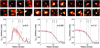 |
Fig. A.1. Stacked cutouts and SFR surface density profiles. Top: median stacked cutouts at the position of the QGs in the three redshift bins, at 24 μm (Spitzer/MIPS), 100 and160 μm (Herschel/PACS), 250, 350 and 500 μm Herschel/SPIRE, 850 μm (JCMT/SCUBA-2) and 1.1 mm (ASTE/AzTEC). The white line in each panel has a length of 15”, while the green circles show the beam FWHM in each band. Bottom: Normalised, average SFR surface density (ΣSFR) profile of the satellites of QGs (circles) in various redshift bins. The error bars correspond to the standard deviation of the surface density in each bin. The pink lines and the shaded regions show the best-fit ‘quenched’ β-models to ΣSFR and their uncertainties. The vertical grey lines denote the half-width at half-maximum of the MIPS and SPIRE beams. |
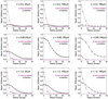 |
Fig. A.2. 1D profiles of the auto-correlation and satellite signal, showing their respective amplitudes (in arbitrary units) at 24, 100 and 160 μm. The autocorrelation signal includes the central point source since one fitted amplitude is used for both (see Sect. 3). |
This method makes the implicit assumptions that the SED-derived obscured SFR and FIR emission of satellites have the same spatial distributions, and that satellites below the detection threshold of the multi-wavelength Laigle et al. (2016) catalogue are similarly distributed as their brighter counterparts. On the other hand, we note that the median mass of satellites
increases somewhat at radii r < 10″, which suggests that sub-threshold (i.e. lower mass) satellites contribute less signal at small radii. This might result in a slight underestimate of the FIR flux of the central QG. Fig. A.3 shows, for the three redshift bins, the total measured FIR signal (after background subtraction, and bias correction as in Béthermin et al. 2015) and its decomposition in SF satellite and QG components (the latter after subtraction of the autocorrelation term). The values of each component in each band along with the corresponding uncertainties are listed in Table A.1.
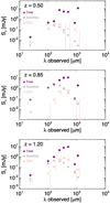 |
Fig. A.3. Background-subtracted and bias-corrected FIR SEDs, before and after decomposition in SF and QG components: total signal (purple), SF satellites (grey), and QG with error bars on the side (light pink). Only the point-source component of the QG SED is shown (that is, after subtraction of the autocorrelation term). As described in Sect. 3, the satellite points are fitted to the data at ≤160 μm and extrapolated from Magdis et al. (2012) templates at longer wavelengths. |
Stack decomposition.
Appendix B: Robustness of the sample selection
To investigate the dependency of our results on the selection criteria used to build the three samples, and in particular to conclusively exclude a non-quiescent origin for the FIR signal found, we performed the analysis on sub-samples drawn from the main one using the following a ‘conservative’ colour cut that adds a 0.1 mag margin to the NUVrJ, rJK, and BzK quiescent loci used to select QGs (Fig. B.1, top). This was intended to further minimise the possibility of contamination of the sample by dusty SFGs close to the edge of the quiescent region. This yielded 909, 1241, and 415 objects in the high-, mid-, and low-z redshift bins, respectively, corresponding to a reduction by 35%, 19%, and 26%. Finally, supplementary ‘blue’ and ‘red’ cuts, in which the quiescent loci in NUVrJ space were split perpendicular to the dividing line so as to generate approximately equal-size sub-samples (Fig. B.1, bottom) we applied.
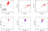 |
Fig. B.1. Sample selection tests. Top:NUVrJ, BzK, and rJK colour diagrams with a conservative 0.1 mag margin (red lines) added to prevent contamination from reddened star forming objects. Bottom: low-, mid-, and high-z samples divided into blue and red sub-samples in NUVrJ colour space. |
Stacked cutouts were produced and fluxes were extracted following the method described in Sect. 3, while the resulting FIR SEDs were modelled as in Sect. 4. Despite the lowered S/N due to the reduced sample sizes, we found that the SEDs of the sub-samples were consistent, within their uncertainties, with those of the full samples. This is further confirmed by the parameters produced by the fit, which do not deviate appreciably with those listed in Table 1. In particular, those derived from the blue and red sub-samples are entirely consistent with each other. Consequently, we conclude that the latter are not the product of either contamination by non-quiescent objects, or due a particular population of QGs within the main sample.
Appendix C: Estimate of the AGN duty cycle
After subtracting the star-forming radio slope, estimated from the FIR-radio correlation (Delhaize et al. 2017), the average excess at 1.4 GHz in the high-, mid-, and low-z bins corresponds to intrinsic luminosities of 2.2 × 10²², 7.0 × 10²¹, and 5.2 × 10²¹ W Hz−1, respectively. We also add to these the 5.4 × 10²² W Hz−1 1.4 GHz excess from the z ∼ 1.8 sample of G18. To translate these excess fluxes extracted from median stacks into an AGN fraction, we considered the evolving 1.4 GHz AGN luminosity functions of Novak et al. (2018), evaluated between 1022 and 1028 WHz. We first noted that the G18, high-, mid-, and low-z excesses correspond respectively to > 1, 0.59 ± 0.9, 0.19 ± 0.04, and 0.14 ± 0.02 times the integrated AGN luminosity function. However, this does not account for the sampling of the redshift bins nor the non-zero noise of the original data used to make the stacks (about 0.015 μJy beam−1; Schinnerer et al. 2010), which can impact the median flux. We performed a set of 1000 simulations based on random samplings of the Novak et al. (2018) luminosity function, with sample sizes and redshift distributions corresponding to our three redshift bins. For each simulation the duty cycle was then varied from 0 to 100%, with ‘off’ AGNs set to zero luminosity. Finally, we added Gaussian noise to each object based on the r.m.s. of the data, converted to intrinsic luminosities. This yielded duty cycles of  ,
,  ,
,  , and
, and  for the G18, high-z, mid-z, and low-z quiescent stacks, respectively.
Appendix D: Simulation of FIR parameters
To investigate the uncertainties and possible systematic effects in the derivation of the Mdust and LIR estimates introduced by the available photometry of our stacked SEDs as a function of the intrinsic shape of the SED, we performed bootstrapping simulations. We first built the full set of DL07 models ranging from Umin = 0.1 to 50 with a fixed LIR and Mdust. We then redshifted each template to the central redshift of each of our redshift bins and measured its synthetic photometry in all the available bands covered by our stacking analysis. To mimic our observations from the emerging set of 8 photometric data points (24 μm–1.1 mm), we added a random fluctuation in each band of up to 20% and randomly selected and placed at S/N = 3 four data points between 24 − 1100 μm. In the process, we ensure that the data set included one data point at observed 24 μm and one data point in the R-J tail, but not longer than λrest ≈ 220 μm, as is the case for all of our observed stacks. The remaining bands were placed at S/N = 1 and treated as upper limits. Following this procedure, we constructed 100 sets of synthetic photometry for each Umin and performed SED fitting using the same methodology as that applied to our observations. The comparison between in output and input Mdust and LIR for each template is presented in Fig. D.1. It is evident that the uncertainties become more severe for the coldest templates. This is expected since for the coldest templates with the lowest Umin the  m is moving closer to the peak of the SED, leaving the R-J tail less constrained, with implications on the derived Mdust. Nevertheless, we see that for the combination of the data points considered here, there are no systematic effects in the derivation of Mdust and LIR.
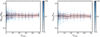 |
Fig. D.1. Simulations on the derivation of Mdust and LIR. The ratio of derived over input Mdust (left) and LIR (right) as a function of intrinsic ⟨Umin⟩ for a range of simulated DL07 models mimicking the dynamical range and S/N of the available photometry for our stacked SEDs. For each Umin template the data are colour coded by the density of the points. The pink shaded region encloses the 68% of the derived ratios. Noticeably, the range of the output/input ratios, and thus the corresponding uncertainties are larger for colder templates (Umin < 5.0). |
All Tables
Stacked photometry of the QG population, as derived through flux density decomposition.
All Figures
|
Fig. 1. Redshift ranges for an efficient use of the BzK and rJK colour diagrams. Left:BzK diagram for the selection of 0.3 ≤ z < 1.0 QGs. The yellow, blue, and red contours represent the loci of stars, SFGs, and QGs at 0.3 ≤ z < 1.0 selected by the NUVrJ + BzK selection. Sources with a 3σ detection at 24 μm in Jin et al. (2018) have been excluded. The black lines represent the original cuts by Daddi et al. (2004) to select galaxies at 1.4 ≲ z ≲ 2.5. The red lines show our cut at low redshifts (Eq. (1)). For reference, the tracks show the synthetic colours for the 13 Gyr elliptical (E), early-type spirals (Sa), and M82-like templates by Polletta et al. (2007), as marked in the labels. The colours are computed for 0.3 < z < 1.5 in step of Δz = 0.3. No evolutionary effects are included. The black segments show the reddening vectors at z = 0.3, 1, and 2. Right:rJK diagram for the selection of 1.0 ≤ z < 1.4 QGs. The yellow, blue, and red contours represent the loci of stars, SFGs, and QGs at 1.0 ≤ z < 1.4 selected by the NUVrJ + rJK selection. The remaining lines are coded as in the left panel. |
| In the text | |
|
Fig. 2. Selection and binning. Left: grey points showing the final sample of double-colour selected and 24 μm faint QGs in the redshift vs. stellar mass plane. The rose area and the black grid mark the limits of the bins used to group galaxies for stacking. The number of stacked sources per bin are displayed. The red line indicates the 90% stellar mass completeness limit for QGs in the ‘deep’ UltraVISTA sample (Laigle et al. 2016), adjusted for the different IMF. Right: blue points showing the position of the stacked massive QGs (M* > 1010.8 M⊙) in the redshift vs. sSFR(UV) plane. The error bars on the redshift indicate the width of the bins. Only the statistical uncertainties on sSFR(UV) are shown on the y-axis. The solid red line indicates the 3σ detection limit for Spitzer/MIPS at 24 μm (σ = 15 μJy, Jin et al. 2018) converted to SFR using the MS templates from Magdis et al. (2012) and assuming M* = 1011.2 M⊙, matching the median stellar mass of our sample in each redshift bin. The grey shaded area and the grey line indicate the location of the MS and its 0.3 dex scatter, computed for a galaxy with M* = 1011.2 M⊙. |
| In the text | |
|
Fig. 3. Observed median IR SEDs of massive QGs. The magenta circles mark the observed photometry, with arrows indicating 3σ upper limits for bands where the measured flux density was negative. We note that the radio points at 10 and 20 cm were not included in the modelling. The black line and the grey shaded areas indicate the best-fit model from the Draine & Li (2007) templates and the associated uncertainty. The dashed orange line is the best fit adopting a single Td modified black body. The left, middle, and right panels show the results for the redshift intervals 0.3 < z < 0.65, 0.65 < z < 1.0, and 1.0 < z < 1.4, respectively. Salient properties of the sample are reported in Table 1. |
| In the text | |
|
Fig. 4. Evolution of the dust to stellar mass ratio and of the gas fraction of QGs. The filled blue circles mark the Mdust/M* of the stacked QGs in the 0.3 < z < 2.0 range, including the results from G18. The grey shaded region depicts the trend for MS galaxies from Kokorev et al. (2021). The orange shaded region captures the range of Mdust/M* for local QGs, as drawn from the literature (see text). The dotted blue line (blue shaded region) corresponds to the best fit (scatter) to the 0.0 < z < 1.0 Mdust/M* data of QGs, with a functional form of Mdust/M* ∝ (1 + z)5.0. The bold, dashed purple line (shaded region) depicts the evolution (scatter) of Mdust/M* (and of fgas) as derived from the progenitor bias analysis of Gobat et al. (2020), which is discussed in Sects. 5.2 and 6. The conversion of Mdust/M* to fgas assumes solar metallicity and GDR = 92. |
| In the text | |
|
Fig. 5. Gas depletion timescales. Left: gas depletion time scale (tdep) as a function of SFR. The blue (grey) circles correspond to the stacked samples of QGs for the case of solar (super solar) metallicity, assuming GDR = 92 (35). The dashed grey line and the grey shaded region depict the trend for MS galaxies from Sargent et al. (2014) with a scatter of 0.23 dex. The magenta shaded region marks the area with τdep < 100 Myr, typical of star-bursting galaxies. Right: gas depletion time scale as a function of redshift. The symbols are the same as in the left panel. The dashed grey line and the grey shaded region depict the trend of Liu et al. (2019) for MS galaxies at fixed M* = 2 × 10¹¹ M⊙ and its corresponding scatter of 0.23 dex. |
| In the text | |
|
Fig. 6. Dust temperatures and average SED. Left: the evolution of Td in QGs. The filled blue circles mark the luminosity-weighted Td for the stacked QGs at 0.3 < z < 2.0, including the results from G18. Filled grey triangles and squares indicate SFGs on the MS and strong starbursts from Béthermin et al. (2015). Filled and open grey circles represent the mass-averaged values and the most massive galaxies (11.0 < log(M*/M⊙) < 11.5, Salpeter IMF) for the star-forming sample of Schreiber et al. (2018a), respectively. The solid and dashed grey lines indicate the best fit models from Schreiber et al. (2018a) and Béthermin et al. (2015), extending the parameterisation of Magdis et al. (2012). The dotted grey line indicates the expected Td track for a size evolution of QGs, R ∝ (1 + z)−1.48. The track is normalised to the Td of the z = 1.8 sample. Right: composite and template FIR SED for z > 0 QGs. The magenta circles (arrows) correspond to the photometry (3σ upper limits) of the stacked ensembles presented in Fig. 3 normalised to LIR = 1010 L⊙ (and Mdust = 1.11 × 10⁸ M⊙). The DL07 and MBB model fits to the SED are shown with grey and red dashed lines. The dotted blue line correspond to the typical SED of z = 1.0 MS galaxies from Magdis et al. (2012), normalised to the same LIR. The QG template is publicly available at www.georgiosmagdis.com/software/. |
| In the text | |
|
Fig. 7. ALMA outlook and systematics. Left: ALMA flux densities in various bands for an evolving fgas as (1 + z)5.0 at 0.0 < z < 1.0 and fixed fgas = 8%, at z > 1.0. The predicted fluxes are derived using the average DL07 SED presented in Fig. 6(right) and are corrected for CMB effects. The blue shaded region depicts the range of predicted flux densities in ALMA Band 3 assuming a 50% uncertainty in the adopted fgas. Middle: ratio of Mgas estimates, as inferred for a fixed monochromatic luminosity at a given rest-frame wavelength from (1) scaling the average SED of QGs presented in Fig. 6(right), |
| In the text | |
|
Fig. A.1. Stacked cutouts and SFR surface density profiles. Top: median stacked cutouts at the position of the QGs in the three redshift bins, at 24 μm (Spitzer/MIPS), 100 and160 μm (Herschel/PACS), 250, 350 and 500 μm Herschel/SPIRE, 850 μm (JCMT/SCUBA-2) and 1.1 mm (ASTE/AzTEC). The white line in each panel has a length of 15”, while the green circles show the beam FWHM in each band. Bottom: Normalised, average SFR surface density (ΣSFR) profile of the satellites of QGs (circles) in various redshift bins. The error bars correspond to the standard deviation of the surface density in each bin. The pink lines and the shaded regions show the best-fit ‘quenched’ β-models to ΣSFR and their uncertainties. The vertical grey lines denote the half-width at half-maximum of the MIPS and SPIRE beams. |
| In the text | |
|
Fig. A.2. 1D profiles of the auto-correlation and satellite signal, showing their respective amplitudes (in arbitrary units) at 24, 100 and 160 μm. The autocorrelation signal includes the central point source since one fitted amplitude is used for both (see Sect. 3). |
| In the text | |
|
Fig. A.3. Background-subtracted and bias-corrected FIR SEDs, before and after decomposition in SF and QG components: total signal (purple), SF satellites (grey), and QG with error bars on the side (light pink). Only the point-source component of the QG SED is shown (that is, after subtraction of the autocorrelation term). As described in Sect. 3, the satellite points are fitted to the data at ≤160 μm and extrapolated from Magdis et al. (2012) templates at longer wavelengths. |
| In the text | |
|
Fig. B.1. Sample selection tests. Top:NUVrJ, BzK, and rJK colour diagrams with a conservative 0.1 mag margin (red lines) added to prevent contamination from reddened star forming objects. Bottom: low-, mid-, and high-z samples divided into blue and red sub-samples in NUVrJ colour space. |
| In the text | |
|
Fig. D.1. Simulations on the derivation of Mdust and LIR. The ratio of derived over input Mdust (left) and LIR (right) as a function of intrinsic ⟨Umin⟩ for a range of simulated DL07 models mimicking the dynamical range and S/N of the available photometry for our stacked SEDs. For each Umin template the data are colour coded by the density of the points. The pink shaded region encloses the 68% of the derived ratios. Noticeably, the range of the output/input ratios, and thus the corresponding uncertainties are larger for colder templates (Umin < 5.0). |
| In the text | |
Current usage metrics show cumulative count of Article Views (full-text article views including HTML views, PDF and ePub downloads, according to the available data) and Abstracts Views on Vision4Press platform.
Data correspond to usage on the plateform after 2015. The current usage metrics is available 48-96 hours after online publication and is updated daily on week days.
Initial download of the metrics may take a while.