| Issue |
A&A
Volume 646, February 2021
|
|
|---|---|---|
| Article Number | A32 | |
| Number of page(s) | 17 | |
| Section | Numerical methods and codes | |
| DOI | https://doi.org/10.1051/0004-6361/202038293 | |
| Published online | 02 February 2021 | |
Optimal extraction of echelle spectra: Getting the most out of observations
1
Department of Physics and Astronomy, Uppsala University, Box 516, 75120 Uppsala, Sweden
e-mail: This email address is being protected from spambots. You need JavaScript enabled to view it.
2
INASAN, 119017 Pyatnitskaya str., 48, Moscow, Russia
Received:
29
April
2020
Accepted:
18
November
2020
Abstract
Context. The price of instruments and observing time on modern telescopes is quickly increasing. Therefore, it is worth revisiting the data reduction algorithms to extract every bit of scientific information from available observations. Echelle spectrographs are typical instruments used in high-resolution spectroscopy, but attempts to improve the wavelength coverage and versatility of these instruments has resulted in a complicated and variable footprint of the entrance slit projection onto the science detector. Traditional spectral extraction methods generally fail to perform a truly optimal extraction when the slit image is not aligned with the detector columns and, instead, is tilted or even curved.
Aims. Here, we present the mathematical algorithms and examples of their application to the optimal extraction and the following reduction steps for echelle spectrometers equipped with an entrance slit that is imaged with various distortions. The new method minimises the loss of spectral resolution, maximises the signal-to-noise ratio, and efficiently identifies local outliers. In addition to the new optimal extraction, we present order splicing and a more robust continuum normalisation algorithm.
Methods. We developed and implemented new algorithms that create a continuum-normalised spectrum. In the process, we account for the (variable) tilt or curvature of the slit image on the detector and achieve optimal extraction without prior assumptions about the slit illumination. Thus, the new method can handle arbitrary image slicers, slit scanning, and other observational techniques aimed at increasing the throughput or dynamic range.
Results. We compare our methods with other techniques for different instruments to illustrate the superior performance of the new algorithms compared to commonly used procedures.
Conclusions. Advanced modelling of the focal plane requires significant computational effort but it has proven worthwhile thanks to the retrieval of a greater store of science information from every observation. The described algorithms and tools are freely available as part of our PyReduce package.
Key words: instrumentation: spectrographs / methods: data analysis / techniques: spectroscopic / methods: numerical
© ESO 2021
1. Introduction, motivation, and history
Nearly 20 years ago, one of our authors joined Jeff Valenti in creating an algorithm for the optimal extraction of echelle spectra without prior assumptions about the cross-dispersion profile. Initially, the math was presented only for the case when the slit image is perfectly aligned with the detector columns, but a brave promise to extend this in the future to tilted and curved slit images was made. Just 18 years after the original paper was published (Piskunov & Valenti 2002), we offer this work with the aim of delivering on this promise.
The purpose of this paper is to describe the current status of the data-processing package REDUCE, which has become fairly popular for extracting 1D wavelength-calibrated spectra from data taken with cross-dispersed echelle spectrometers. Such instruments combine a high level of efficiency with high spectral resolution, but the need for an angular separation of spectral orders (cross-dispersion) makes data extraction notoriously difficult since spectral orders in the focal plane have variable spacing and shape. In slit instruments, the direction of the main dispersion is not perpendicular to the spatial direction (slit image) and in Non-Littrow optical schemes (von Littrow 1863; Kerschbaum & Müller 2009), the slit images often exhibit variable tilt and even curvature across the focal plane. Here we define the ‘optimality’ of the extraction in terms of maximising the signal-to-noise ratio (S/N) per resolution element, while preserving the spectral resolution delivered by the optical system. Our original optimal extraction was presented together with several other algorithms (that now make up the core of the REDUCE package) in Piskunov & Valenti (2002); henceforth we refer to that work as Paper I.
The originality of our approach, as presented in Paper I, is that we fit a 2D model to the 2D data in a least squares sense. This is unlike many other optimal extraction algorithms, which effectively perform summation in the spatial direction only. Such a summation requires weights to minimise the accumulated noise (Horne 1986). The purpose of weights is to balance the contribution of residuals involving measurements with different uncertainties. Uncertainties could be estimated either by assuming the analytical form of the cross-dispersion profile or by constructing this profile empirically (e.g. Petersburg et al. 2020). In any case, this implies that the model is ‘perfect’ and the model will match exactly – with infinitely small uncertainties the data. Unfortunately, we do not expect this to happen for a number of reasons ranging from very primitive adjustments for optical aberrations to the somewhat arbitrary selection of parameters for the slit function definition (see below). Thus, using observational uncertainties may give disproportional weight to data points located on the highest curvature parts of the cross-dispersion profile. Therefore, at this point, we chose not to use additional weights in the least-squares fitting of the data based on the fact that each pixel contribution is weighted by the cross-dispersion profile and by the spectrum.
We call our optimal extraction algorithm “slit decomposition” as it decomposes a 2D image registered by the focal plane detector into two vectors: a spectrum and a slit illumination function. We make no assumptions about the shape of the slit illumination function (also known as the cross-dispersion profile; see below for more details). The original algorithm had several limitations that took some effort to sort out. One major restriction was the assumption that the spectrometer creates a rectangular slit image for each wavelength and that it is strictly parallel to the pixel columns on the detector. Another restriction was the use of IDL as the programming language. Yet another was the insufficiency of the speed optimisation strategy. When Paper I was published, certain tools (e.g. the wavelength calibration and continuum normalisation) did not even exist. Several other implementations of the optimal extraction algorithm exist (e.g. Marsh 1989; Cushing et al. 2004; Cui et al. 2008; Zechmeister et al. 2014; Petersburg et al. 2020), but this is the first one to allow for a slit function that is not aligned with the detector columns.
Since the release of Paper I, the ‘perfect’ extraction (also known as ‘spectro-perfectionism’) method has been developed (Bolton & Schlegel 2010; Cornachione et al. 2019). While the method was designed for the recovery of faint objects, it can also be used in stellar spectroscopy. It is however much more computationally expensive and suffers from several other practical difficulties. Most importantly, the algorithm relies on knowledge of the point spread function (PSF) shape at any given wavelength, which is difficult to determine accurately. This also means that any instrument shift will need to be corrected. We note that REDUCE has no concept of wavelength or PSF created by diffraction (and thus its limitation), but by working with pixels, it can easily accommodate drifts between calibrations and science exposures, in terms of both spatial and dispersion directions. This follow-up study gives us an opportunity to catch up with the development of REDUCE, that is, to write up the math behind the main algorithms and speed optimisation concepts and compiling it all in one place.
In the next three sections of the paper, we present the algorithms of optimal extraction in the case of a tilted and curved slit image (Sect. 2), the determination of the slit image geometry (Sect. 3), the 1D and 2D wavelength calibration methods and their comparison (Sect. 4), and the continuum normalisation (Sect. 5). Then we present the Python and C implementation of the main algorithms, along with some examples illustrating the performance of the latest version of REDUCE in terms of the quality of the data reduction (Sect. 6).
2. Generalised slit decomposition algorithm
We start this section by reminding the reader, and ourselves, of the algebra required to decompose (a fragment of) a spectral order image created by an echelle spectrograph on a matrix detector. We represent the image as an outer product of two vectors: the sLit illumination function L and the sPectrum P. In the following, our convention is based on the notion that the main dispersion is ‘approximately’ aligned with the detector rows, while the cross-dispersion or spatial direction ‘approximately’ follows the columns.
In addition to a 2D image of a spectral order sampled on the detector, we also need the trace of the order, namely, the location of the spectral order in the pixel coordinate system. We presented a robust algorithm for order tracing in Paper I. The image itself is supposed to be corrected for bias, dark current, and other types of background (e.g. by combining nodding images for infrared observations) and flat-fielded. To avoid noise amplification we use the so-called ‘normalised’ flat field (as per Paper I). The normalised flat field is the flat field data (usually a master flat) divided by the flat field model constructed by the slit decomposition algorithm from the cross-dispersion profile and the blaze function. In places where the flat field signal is low (e.g. between spectral orders) the ratio is set to one to avoid introducing additional noise. Thus, the normalised flat contains only positive values around one. It carries the information about relative pixel sensitivity and is not affected by the signal variation in the original master flat. This is particularly important for the fibre-fed instruments, where the flat field signal decreases quickly in the direction of the cross-dispersion.
Usually, we process the whole spectral order in a sequence of overlapping rectangular segments that we call ‘swaths’ (see Fig. 1 for illustration). Using swaths instead of the whole order allows us to account for changes in the slit illumination function, which is held constant within each swath. The shorter the swaths, the more variability in the slit illumination function along the spectral order can be reproduced, replicating optical aberrations and optical imperfections. On the other hand, for low S/N data, wider swaths make the decomposition more robust and help to extract the available signal.
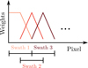 |
Fig. 1. Distribution of the first three swaths in an order. Each swath is overlapped by two other swaths (except for the first and last swath), so that each pixel is contained in two swaths. The swaths are combined into the final spectrum using linear weights with the central pixels having the most weight. |
The vertical (cross-dispersion) extension of the swaths is determined relative to the order trace using two parameters: the number of pixels below and above the trace. This provides practical flexibility in case the image used for order localisation has an offset relative to the science image. REDUCE offers a special tool that can estimate the extraction height using the signal level drop in the spatial direction in the central swath or by fitting a cross-dispersion profile with a Gaussian. If neither of the two methods is acceptable, the user can also specify the offset in pixels explicitly. The extraction height should cover only the current spectral order. Extending it further will not change the extraction result. This is because the derived signal is being computed using a model, which is constructed by the slit decomposition and not from the measured pixel counts. Of course, adjacent orders should not be included and we must be aware of the increase in computation time. Using a too narrow height may (and will) affect the quality of the model and, thus, the resulting spectrum as we lose some information. The extraction height selection is illustrated in the top sketch of Fig. 2. Once the central line crosses the pixel row, the initial and final extraction row numbers are shifted accordingly. The vertical size of the swath affects the computational time, so we compress the swath by packing pixels that fall into the extraction range for each column into a rectangular array. Every time the centre line crosses the pixel row, the new central line and the packed array exhibit discontinuity, as shown in the bottom panel of Fig. 2. The order trace line yc(x) is now contained within a single row of detector pixels. We then shift the order trace to the bottom of the pixel row, so that it only has values between 0 and 1.
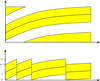 |
Fig. 2. Top: input image with selected order (dashed line) and two adjacent orders. Bottom: image packed for slit decomposition with the discontinuous order trace (dashed line). |
2.1. Problem setup
For an ideal cross-dispersed echelle spectrometer measuring a cosmic (faraway) source, the image of a spectral order consists of many monochromatic images of the entrance slit characterised in the first approximation by the relative intensity distribution in the spatial direction (the slit illumination function). Each slit illumination function is scaled by the relative number of photons in the corresponding wavelength bin (spectrum). Thus, it should be possible to represent a 2D image of a spectral order by two 1D functions and even reconstruct these functions directly from the 2D image registered by the detector pixels.
The goal of the slit decomposition algorithm is to model the 2D intensity distribution in a rectangular area of the detector that contains an image of a spectral order or its fragment. We assume that the detector consists of square, equally spaced and equally sized pixels, and containing no gaps between pixels. This is not strictly true in practice, but neither is it a limiting assumption: it is easy to introduce the physical coordinates and the size of each pixel and use these instead of pixel numbers and pixel contribution in the PSF footprint. We do not do this here because the following algebra is complex enough even without this extra layer of transformation. Thus, in the following, we stick to rows and columns as the coordinates. As mentioned before, we assume the main dispersion direction is roughly horizontal, so that the wavelength inside the order changes in x-direction, while the spatial extension of the slit is approximately vertical. Here, REDUCE provides the transformation mechanism for achieving this orientation for any given instrument. The input for the problem is the 2D photon count surface measured by the detector, Sx, y, and the trace of the order location, yc(x).
2.2. Decomposition in case of the strictly vertical 1D point spread function
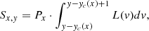
We start by assuming an ideal case where the monochromatic images of the slit are perfectly aligned with the columns of the detector. Then our model for the photon count, Sx, y, on the detector pixel, (x, y), is given by an outer product of the two vectors: a continuous slit-illumination function, L(v), and the discrete spectrum, Px:
 (1)
(1)
where we assume that the central line of the order, yc(x), is known precisely. Also, L drifts vertically across pixels from one column to the next due to the tilt of the spectral order. This is described by the shift of integration limits relative to the detector row, y. The value of the shift is given by the order trace, yc(x). The slit illumination function, L, remains independent of x on the v grid. The spectrum, P, changes from one column to the next. To avoid scaling degeneracy between L and P, we postulate that the area under L should be equal to 1. For infrared (IR) instruments, special care should be taken when using chopping or nodding techniques to avoid the effect of the negative values. Normally, electronic detectors do not generate negative signal. The background signal is removed by subtracting the bias correction. When subtracting images within chopping or nodding pairs, however, it is still possible to get negative values. Preserving these values is important to avoid distorting the noise distribution function (see e.g. Lenzen et al. 2005).
In practice, Eq. (1) will not hold precisely even if all our assumptions are met. This is due to the noise in the observation, ghosts, and scattered light in the spectrometer, cosmic rays, detector defects, etc. Thus, our model will fit the measurements only approximately and for some pixels, it will not fit at all. This means that the model cannot be constructed for each pixel individually, but it must instead be derived from a segment of the image in some sort of least-squares approach. To do so, the slit function must be set on some kind of discrete grid. This grid must be finer than the pixel size if we want to account for a smooth shift of the central line and for a potentially complex structure of L. We can create such a grid by introducing an integer oversampling factor, O, so that 1/O gives the step of the fine grid (or subgrid) in units of detector pixel size. Now we are able to express the requirement for the model to match the data as a least squares minimisation problem:
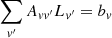
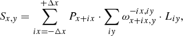
![Mathematical equation: $$ \begin{aligned} \Phi =\sum _{x,{ y}}\! \left[E_{x,{ y}}\! -\! S_{x{ y}}\right]^2= \sum _{x,{ y}} \left[E_{x,{ y}} - P_x\cdot \sum _{ v} \omega _{x{ y}}^{ v}\cdot L_{ v}\right]^2 \! = \! \mathrm{min} , \end{aligned} $$](/articles/aa/full_html/2021/02/aa38293-20/aa38293-20-eq2.gif) (2)
(2)
where Exy are the actual measurements. The tensor,  , is proportional to the fraction of the area of the subpixel, [x, v], that falls inside the detector pixel, [x, y]. That is to say that for a detector pixel, [x, y],
  is equal to 1/O for all v that are fully contained inside this detector pixel and less than 1/O for the two boundary values of v and 0 for all other indices. We would like to point out that due to our selection of the subgrid, the sum of the two boundary values for every x and y is also 1/O. Figure 3 illustrates the properties of
  .
.
 |
Fig. 3. Schematic presentation of the subgrid sampling of the slit illumination function L and the corresponding structure of the ω tensor. On the top is an example of a slit illumination function aligned for column x. L is set on a subpixel scale v (shown at the bottom panel) that may shift relative to the detector pixels from one column to the next. For three pixels in this column centred at row y we show the structure of the corresponding section of |

The tensor, ω, is the key for representing the projection of the monochromatic slit images onto detector pixels with only a slight generalisation that is needed to follow a tilted or even curved slit, which we describe in the sections below. Here, we deal with a strictly vertical slit projection and, thus, we can note a few important properties of ω that may serve as the basis for speed optimisations here and later on. Each detector pixel is sampled by a maximum of O + 1 subpixels of ω that may have non-zero values. Out of these, all intermediate elements are equal to 1/O. The first and the last elements are less than or equal to 1/O, but their sum is equal to 1/O, so that the integrated weight for any detector pixel x, y given by  is equal to 1. There is also a relation between elements of ω for two consecutive values of y: they overlap by one element in v and the sum of these two elements is again equal to 1/O.
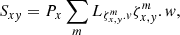
Now we go on to solve Eq. (2). Firstly, we take the two partial derivatives of this equation over the elements of Px and Lv:
![Mathematical equation: $$ \begin{aligned}&\frac{\partial \Phi }{\partial L_{ v}}=-2\sum _{x,{ y}} \left[E_{x,{ y}} - P_x\cdot \sum _{ v} \omega _{x{ y}}^{ v}\cdot L_{ v}\right] P_x\omega _{x{ y}}^{ v} =0, \end{aligned} $$](/articles/aa/full_html/2021/02/aa38293-20/aa38293-20-eq8.gif) (3)
(3)
![Mathematical equation: $$ \begin{aligned}&\frac{\partial \Phi }{\partial P_x}=-2\sum _{x,{ y}} \left[E_{x,{ y}} - P_x\cdot \sum _{ v} \omega _{x{ y}}^{ v}\cdot L_{ v}\right] \sum _{ v}\omega _{x{ y}}^{ v} L_{ v}=0. \end{aligned} $$](/articles/aa/full_html/2021/02/aa38293-20/aa38293-20-eq9.gif) (4)
(4)
These can be re-written as linear equations for Lv and Px:
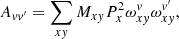
![Mathematical equation: $$ \begin{aligned}&\sum _{{ v}^{\prime }}\left[\sum _{x{ y}}P_x^2\omega _{x{ y}}^{ v}\omega _{x{ y}}^{{ v}^{\prime }}\right]L_{{ v}^{\prime }}=\sum _{x{ y}}E_{x{ y}}P_x\omega _{x{ y}}^{ v}, \end{aligned} $$](/articles/aa/full_html/2021/02/aa38293-20/aa38293-20-eq10.gif) (5)
(5)
![Mathematical equation: $$ \begin{aligned}&P_x\sum _{ y}\left[\sum _{ v}\omega _{x{ y}}^{ v}L_{ v}\right]^2=\sum _{ y} E_{x{ y}}\sum _{ v}\omega _{x{ y}}^{ v}L_{ v}, \end{aligned} $$](/articles/aa/full_html/2021/02/aa38293-20/aa38293-20-eq11.gif) (6)
(6)
or:
 (7)
(7)
![Mathematical equation: $$ \begin{aligned}&P_x=\frac{\sum _{ y} E_{x{ y}}\sum _{ v}\omega _{x{ y}}^{ v}L_{ v}}{\sum _{ y}\left[\sum _{ v}\omega _{x{ y}}^{ v}L_{ v}\right]^2} , \end{aligned} $$](/articles/aa/full_html/2021/02/aa38293-20/aa38293-20-eq13.gif) (8)
(8)
where the expressions for the matrix Avv′ and the right-hand-side (RHS) bv are given by Eq. (5).
Equations (7) and (8) are linear but they cannot be combined to separate the unknowns (see also Horne 1986). Therefore, we adopt an iterative scheme alternating between solving Eqs. (7) and (8). Level of changes in Px can be used as convergence test.
We note that the equation for the spectrum Px includes the slit function Lν as a weight. This property is responsible to maximising the S/N in our algorithm.
The whole procedure can be integrated with a ‘bad pixel’ mask that may be dynamically adjusted during the iterations. Supposing Mxy is 1 for ‘good’ detector pixels and 0 otherwise. We can rewrite the expressions for matrix A and the RHS in Eq. (7) as:
 (9)
(9)
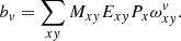 (10)
(10)
Then the equation of Px is:
![Mathematical equation: $$ \begin{aligned} P_x=\frac{\sum _{ y} M_{x{ y}} E_{x{ y}}\sum _v\omega _{x{ y}}^{ v}L_{ v}}{\sum _{ y} M_{x{ y}}\left[\sum _{ v}\omega _{x{ y}}^{ v}L_{ v}\right]^2} . \end{aligned} $$](/articles/aa/full_html/2021/02/aa38293-20/aa38293-20-eq16.gif) (11)
(11)
Massive defects, such as bad columns, must be detected beforehand to avoid divisions by zero. In the iteration loop above, we can implement adjustments of Mxy by constructing the standard deviation between the data and the model as given by Eq. (2), using the current bad pixel map and then correcting the map by comparing the actual difference with the standard deviation.
2.3. Convergence, selection of oversampling, and regularisation
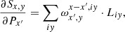
The iterative scheme presented above has excellent convergence properties: typically, the unknown functions are recovered to a relative precision of 10−5 in three to five iterations. The convergence rate, besides a general consistency between the data and model, depends on the selection of O, which deserves a separate discussion. The oversampling is required to adequately describe the gradual shift of the central line relative to the pixel rows of the detector and possible features of the slit illumination. Qualitatively, we would expect O = 1 should be sufficient when a spectral order is strictly parallel to pixel rows. On the other hand, if the central line shifts by 0.5 pixel over the whole swath, then O could perhaps be 2. The problem is that no cross-disperser (the low-dispersion spectrometer used to separate echelle orders) keeps spectral orders in straight lines. This makes it impossible to use a single oversampling value for the whole order. The issue can be alleviated by selecting O to match the largest tilt while regularising Lv. One suitable form of regularisation is applying a constraint on the first derivatives (classical Tikhonov regularisation, Tikhonov & Arsenin 1977) that would damp oscillations of the oversampled slit function. The use of regularisation decouples the selection of the oversampling factor from the exact order geometry. Similarly, we may want to have the option of controlling the smoothness of the spectrum in return for sacrificing its spectral resolution. Such an option is helpful when decomposing the flat field or other sources where no sharp spectral features are expected. Both regularisations can be easily incorporated into Eq. (2):
![Mathematical equation: $$ \begin{aligned}&\Phi =\sum _{x,{ y}} M_{x{ y}}\left[E_{x,{ y}} - P_x\cdot \sum _v \omega _{x{ y}}^{ v}\cdot L_{ v}\right]^2 \\&\qquad +\Lambda _L\sum _{ v} \left(L_{{ v}+1}-L_{ v}\right)^2+\Lambda _P\sum _x \left(P_{x+1}-P_x\right)^2\nonumber , \end{aligned} $$](/articles/aa/full_html/2021/02/aa38293-20/aa38293-20-eq17.gif) (12)
(12)
where ΛL and ΛP are the regularisation parameters for the two unknown vectors. The corresponding changes to the matrix, Avv′, will affect the main diagonal: 2ΛL will be added to all elements except the first and the last only get one additional ΛL. Also, ΛL should be subtracted from all elements on the upper and lower sub diagonals. Equation (6) becomes a tri-diagonal system of linear equations, with 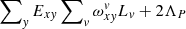 for all x except the first and the last elements where the expression is
  . All subdiagonal elements will contain −ΛP. The use of regularisation for the spectrum is purely optional, while setting ΛL to zero will most probably lead to a zero determinant of matrix Avv′ for O ≫ 1.
The choice of regularisation parameters, ΛL and ΛP, depends on the S/N of the data, the oversampling parameter O, as well as the shape of the slit illumination function. For a reasonable S/N (above 20), it is sensible to set ΛP = 0 and select ΛL as the smallest number that still damps non-physical oscillations in the slit function. Fortunately, the extracted spectrum is not very sensitive to the choice of ΛL. When investigating this issue using ESO UVES, HARPS, and CRIRES+ instrument data with S/N ≈ 50, we discovered that spectra extracted with the best ΛL and 10 × ΛL differ by less than 0.05%.
2.4. Optimisation in case of vertical slit decomposition
Now that the actual slit decomposition is reduced to repeatedly solving a system of two linear equations, we can examine the performance. The typical size of the final systems is given by the packed height of a swath times the oversampling O (typical numbers are 30 × 10) for Lv, and the width of a swath (typically between 200 and 800 columns) for Px. The main complication is the construction of the matrices involved. This process involves the multiplication of a substantially larger tensor  with itself and with Px.
  describes the geometry of the spectral order and thus remains constant throughout the iterations for a given swath. That offers two paths for an efficient construction of the matrices involved in Eqs. (9)–(11).
The first path is to reduce the size of the largest summation using the structure of the ω tensor. Constructing Avv′ (Eq. (9)) is by far the most expensive part of an iteration, but a major part can be pre-computed knowing the order trace line; this part is  . For a given column, x, the 2D projection of
  has a layout similar to the example presented in Fig. 3. We note the self-similar pattern that shifts by O subpixels when moving to the next pixel. A product of two such matrices (that is
  for a fixed x) on a vv′ plane can be evaluated analytically as explained below. Figure 4 shows a typical layout of the ω projection for a fixed x. The structure is self-similar: for each y-column the first non-zero element (from the top of the image) corresponds to L entering the x, y pixel, followed by a set of O − 1 elements in ν with identical 1/O values. The sequence ends with the last value corresponding to leaving pixel, y. For the first y (on the left) the pattern is offset by νmin from the top by the central line yc(x). The next y will have the same pattern offset by an additional O in ν, etc.
 |
Fig. 4. Surface view of a 2D |

We use ‘in’ and ‘out’ to refer to the fractions of the first and the last subpixel of the slit function (referenced with ν) that fall into detector pixel y in column x. Here, the ‘in’ and ‘out’ have values between 0 and 1 and their sum is precisely 1 because we chose for O to be an integer.
The matrix product of  is graphically presented in Fig. 5. This symmetric matrix has repeating square structures around the main diagonal starting at νmin + 1. The side of each square has a length of O + 1. Surprisingly, this matrix contains only seven unique, non-zero elements: two in the corners of the square blocks located on the main diagonal (in ⋅ out/O2 and (in2 + out2)/O2), two in the middle part of the horizontal and the vertical border of each square (in/O2 and out/O2), one in the middle of each square (1/O2), and two in the first and the last non-zero diagonal elements, which are different from the square overlap pixels (in2/O2 and out2/O2) (see Fig. 6). The squares on the main diagonal overlap by one element. The value of all these pixels is the same: (in2 + out2)/O2. The upper left corner of the first square and the bottom right corner of the last square do not overlap with anything, so their values are in2/O2 and out2/O2, correspondingly. Equipped with this knowledge, we can optimise the slit decomposition iterations in the following way.
 |
Fig. 5. Surface view of ω⊤ × ω projection for a fixed x. The result is a symmetric square matrix with a dimensionality of ν. |
(1) We construct the initial guess for the spectrum by, for example, collapsing the input image in the cross-dispersion direction. (2) We construct matrix Avv′ as given by Eq. (9). At this point, we use the insights of this section to generate the product of the two values for ω on the left-hand-side. (3) We evaluate the right-hand-side and solve the Eq. (5) for Lν; We normalise the result, setting the integral of Lν to 1. (4) For each x, we compute  multiplied by the slit function Lν. We use the product to solve for the spectrum Px according to Eq. (8). (5) We evaluate the model image as
 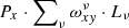 as in Eq. (1). We then compare the model with the input image Exy, find outliers, and adjust the mask. (6) We perform iterations starting from 2° until the change in the spectrum is less than a given margin. We would like to point out that the iterations require re-calculations of neither
  nor of its product
  .
.
2.5. Alternative optimisation strategy
The alternative optimisation approach is based on storing the contributions of every slit function element to a given detector pixel and every detector pixel to a given slit function element. The former tensor is actually very similar to  . We refer to it as
  . Indices x and ν have the usual meaning and the superscript, n, can take one of two values: L (Lower) or U (Upper), corresponding to the cases when an element of the slit function falls onto the boundary of a detector pixel. Each element of tensor ξ has a composite value (a structure). For every combination of indices, it contains the pixel row y, to which subpixel v contributes (we will write it as
  ), as well as the contribution value (footprint) that is between 0 and 1, written as
  . We can see that ξ carries the same information as ω, but it is much more compact since we avoided storing most of the zeros. In addition, ξ needs a counterpart that we call ζ. Each element of
  carries the information about all elements of the slit function affecting detector pixel, xy. The index, m, runs a range between 1 to O + 1 in order to account for the maximum number of contributing subpixels. Like ξ, here, ζ carries two values: the slit function component, ν, referred to as
  and its contribution to pixel x, y,
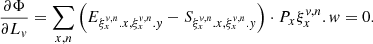
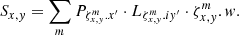
  , which is normally 1/O, except for the boundary subpixels and top and bottom rows of the swath. Both new tensors are, as in the case of ω, only functions of order geometry and, thus, they need to be computed only once. The purpose of these tensors becomes clear once we rewrite Eq. (2) and its derivatives with their help:
 (13)
(13)
![Mathematical equation: $$ \begin{aligned}&\Phi = \sum _{x{ y}} \left[E_{x{ y}}- P_x \sum _m L_{\zeta _{x,{ y}}^m.{ v}}\zeta _{x,{ y}}^m.w\right], \end{aligned} $$](/articles/aa/full_html/2021/02/aa38293-20/aa38293-20-eq39.gif) (14)
(14)
 (15)
(15)
 (16)
(16)
What happens is that the summation is carried out essentially over the non-zero elements of ωTω only. The speed-up can be estimated from Fig. 6 as the ratio of the number of non-zero elements Ny × (O + 1)2 − Ny + 1 to the total number (Ny + 1)2 × O + 1)2. In practice, for a packed swath height of 20 we see a an increase in performance that is a bit more than factor of 20, compared to the direct construction of matrices involved in linear equations.
 |
Fig. 6. Schematic view of the product of ωTω for a fixed value of x. The result is a squared and symmetric matrix of order (Ny + 1) × O + 1 where Ny is the height of the packed swath. The outer side of the ‘squares’ on the main diagonal is O + 1. The squares overlap by one row or column. The offset from the top left corner is determined by the central line: a yc of zero implies vmin = 0. The in and out elements are the footprints of the first and the last subpixels that fall in a given detector pixel x, y. A central line offset of zero would set in = 1 and out = 0. All elements outside the main diagonal boxes are zero. The values inside a box are known explicitly as shown on the sketch. |
The first optimisation path, based on the analytical construction of ωTω results in an even better performance (involving a gain of around another 20% at the expense of greater memory usage), but unlike the 2nd path, its advantage vanishes when we introduce a bad pixel mask as in Eqs. (9)–(11). The mask is involved in computing the product of ωTω, forcing the re-computation of this product during every iteration. Thus, we do not use this approach for the case of a tilted or curved slit image.
2.6. Decomposition in case of a curved and tilted 1D point spread function
In this section, we explore the decomposition of a 1D slit bent by a known amount relative to the detector columns. We assume, thus, that the offset of monochromatic images of the slit from a vertical line on the detector is described by a second order polynomial:

where δy = y − yc(x), with yc(x) being (again) the central line of the order on the detector. We postulate that the offset from column x at the level of the order trace y = yc(x) is zero. This means that c(x) is always 0. In the case of a strictly vertical slit image, the offset expression is reduced to a trivial δx(δy) = 0. For a straight but tilted slit image, we have only the linear term: δx(δy) = b(x)⋅δy. The presence of a horizontal offset means that subpixels may now contribute to adjacent columns, changing the structure of the ω tensor. Therefore the model for detector pixel x, y should be modified to reflect this:
 (17)
(17)
where Δx = ⌈δx⌉ is the pixel range affected by the curvature. Compared to the previous section we are now using the index name, iy, to address the elements of L instead of v in order to emphasise the difference between offsets in x and y directions.
Tensor ω acquired an extra dimension to reflect the contribution to the detector column(s) adjacent to x. In practice, the size of ω does not have to increase dramatically (typically by a factor of 3) since the height of the slit illuminated by a point source is generally small and even a noticeable slit curvature would not result in a large offset in dispersion direction. In long-slit observations, we would not want to use slit decomposition to keep the spatial information. Notable exceptions include the use of an image slicer with many (5–7) slices or an IR spectrum that is a combination of the two nodding positions. We would also like to point out that the column index x of the generalised ω follows the spectrum, P, but since we are interested in the contribution of Px + ix to the pixel, x, in Eq. (17), the offset index, ix, has the opposite sign to the difference between the contributing column (x + ix) and the column (x) (the column, for which the model is constructed).
Partial derivatives of the model Sxy are:
 (18)
(18)
 (19)
(19)
As for the vertical slit case we can formulate the optimisation problem for matching the model to (a fragment of) a spectral order Ex, y:
 (20)
(20)
However, there is no more a one-to-one correspondence between the measured swath and the data needed for the model. This is obvious from Fig. 7: if the black squares represent the selected swath then clearly the model of the first and last columns requires spectrum Px values that cannot be reliably derived from this swath (partial slit images). Overlapping zones would solve this problem by carrying the values of Px from one swath to the next.
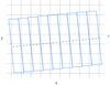 |
Fig. 7. Schematic view of ‘ideal’ monochromatic images of a slit projected onto a detector by a non-Littrow spectrometer. Black squares represent spectrometer pixels. The dashed line traces the centre of a spectral order and the blue boxes show the idealised footprints of slit images. We note that by design the centre of the spectral order and the sides of a slit image intersect at the pixel column boundaries of the detector. |
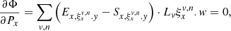
The necessary condition for a (local) minimum is the first derivatives resulting in zero:
 (21)
(21)
 (22)
(22)
Substituting Eqs. (17)–(19) into the last two equations, we get systems of linear equations for P and L:
 (23)
(23)
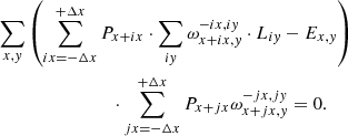 (24)
(24)
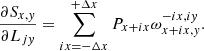
Now we go on to re-organise Eq. (23) by first substituting x with x′+jx, then dropping ’prime’ and finally shifting the measured data part to the right-hand side:
 (25)
(25)
Renaming x′ means that the derivative has been taken over Px rather than over Px′.
Finally, we would like to point out that Eq. (25) is actually a system of Ncols linear equations numbered by the value of x. The matrix for the system is band-diagonal but not symmetric with the width of the band equal to 4 ⋅ Δx + 1.
The system of equations for L is derived in a similar way:
 (26)
(26)
In this case, the matrix of the system is fully filled but symmetric.
2.7. Decomposition optimisation in case of the curved slit
The optimisation follows the second path presented for the vertical slit case. Again, we define two sets of tensors. One (like ω) describes the contribution(s) of subpixel iy, associated with the spectrum centred on detector pixel x, to other detector pixels. As before, we name it ξ. And as before, it has three indices, but now the second superscript runs through four options, reflecting the cases when a subpixel is projected onto the intersection of four detector pixels. With the slit image no longer aligned with the detector columns, a subpixel can project onto two columns and occasionally on a boundary between rows. Thus, subpixel iy can have a footprint in two or even four detector pixels, which are referenced as ![Mathematical equation: $ \xi_{x}^{i\mathit{y},[LL/LR/UL/UR]} $](/articles/aa/full_html/2021/02/aa38293-20/aa38293-20-eq53.gif) . LL, LR, where UL and UR refer to the affected detector pixel location (lower-left, lower-right, upper-left, or upper-right) relative to the selected subpixel.
. LL, LR, where UL and UR refer to the affected detector pixel location (lower-left, lower-right, upper-left, or upper-right) relative to the selected subpixel.
For each combination of indices, the value of  is a structure containing {x′,y′,w}. Here, {x′,y′} are the coordinates of the affected detector pixel and w is the footprint of subpixel {x, iy} inside pixel x′,y′. Tensor ξ will also be very useful when evaluating partial derivatives.
The other tensor, ζ, is in some sense the inverse of ξ. It also has three indices,  , where m indexes the contributing subpixels and has a range between 0 and (O + 1) × 2. For each combination of indices the value of ζ is a structure containing the two coordinates of the contributing subpixel and its weight (footprint) {x′,iy′,w}.
Equipped with these new tensors, we can rewrite the expression for Sx, y as well as the derivatives of Φ.
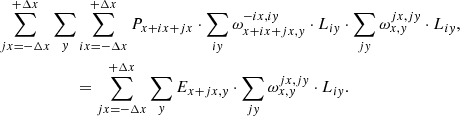
Our model for detector pixel x, y can now be expressed as:
 (27)
(27)
Unlike Eq. (17) we ended up with a single summation.
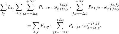
For partial derivatives over Px, we keep only those pixels receiving a contribution from the slit image centred on the {x, yc(x)} position on the detector:
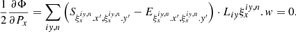 (28)
(28)
The analogous expression for the derivatives over Liy is also easily written with the help of tensor ξ:
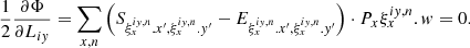 (29)
(29)
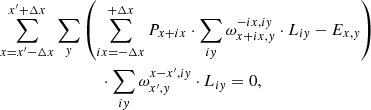
Substituting Eqs. (27)–(29), and moving the part with the measured detector pixel counts to the right-hand side, we get the final form of the system of equations for Px and Liy:
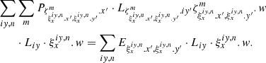 (30)
(30)
 (31)
(31)
The software implementation for Eqs. (30) and (31) faces two challenges: the construction of ξ and ζ tensors and the construction of the matrices and RHSs. The first is solved through a single loop over all subpixels of L for each column x. In this loop, we can record detector pixel coordinates and the corresponding footprints, which are stored by ξ. In the same loop for each detector pixel, we record the coordinates of the contributing subpixel and its footprint, filling the ζ tensor.
The second challenge comes from the fact that the indexing of the unknown vectors (P and L) in Eqs. (30) and (31) is not sequential. We should regard this as a permutation of rows and columns in the linear systems of equations A ⋅ x = y. The equation permutation needs to be stored in order to recover the correct order of elements in the unknown vectors.
Finally, at the horizontal ends of the swath, in some rows, the slit image can (due to the tilt) stretch outside the data fragment, as schematically shown in Fig. 7. The simplest way to handle this issue is to pad each swath with additional columns on both sides and then clip the extracted spectrum by the corresponding amount. At the edges of the detector padding is not possible, which may require the clipping of the extracted spectrum.
2.8. Uncertainties of extracted spectra
The extraction procedure described above can be seen as an inverse problem of a convolution type. It helps to avoid complications due to the degeneracy between P and L or noise amplifications in areas of low signals. Error propagation is notoriously difficult for inverse problems, since the measured noise is known for the result of the convolution i.e. data, while the model statistics is a priori unknown, as is the transformation from detector pixels to the P, L space. Thus, we take on a different approach. Once we have a converged model for a given swath, we can construct the distribution of the difference between observations and model for the whole swath and for each ‘slit image’ realisation, indexed by column number x. The full swath distribution is obviously better defined, so we fit a Gaussian to it. The standard deviation for this Gaussian can be compared to the Poisson estimate using the extracted spectrum P.
To illustrate the procedure, we use a challenge suggested by the referee and used a CARMENES (Quirrenbach et al. 2016) near infrared (NIR) spectrum of HD209458 (car-20180905T23h01m44s-sci-czes-nir). We selected spectral order 18, which has some columns with high signals as well as some with no apparent stellar continuum due to the strong water absorption in the Earth’s atmosphere. Figure 8 shows the application of vertical slit decomposition and how uncertainties of the extracted spectrum are estimated. We use columns 854-1193 of order 18 (0th order is at the bottom) as an example of the first detector in the NIR arm of CARMENES. The standard deviation estimated for the whole swath using the histogram of the data-model differences (panel in the middle right) is nearly identical to the mean Poisson statistics estimate  . The panel below uses a similar approach for individual slit images as indexed by the column number. The plot shows two different estimates for the signal-to-noise ratio. The black line is the square root of the extracted spectrum, that is, a simple Poisson distribution, while the mean deviation between the data and the model weighted by pixel contribution to the given slit image is plotted in red. The noticeably higher level of the uncertainty estimate from the slit decomposition (lower S/N) is real. It reflects the shortcut we took in this test extraction by ignoring the effective ‘tilt’ of the slit image created by the image slicer (two half-circle images of the input fibre), which is seen clearly in the differences (right panel in the 2nd row). While the amplitude of the difference is small, it still drives up our uncertainty estimates. The impact on the extracted spectrum is negligible, as illustrated by the bottom panel of Fig. 8, where we compare our extraction with the standard CARMENES pipeline output. The two extracted spectra agree to 0.1%, if we ignore a few ‘bad pixels’ that are present in this swath.
 |
Fig. 8. Slit decomposition uncertainties. The top four panels show the 2D image of the data as registered by CARMENES (Ex, y in equations), the model reconstructed using the deduced P and L functions (Sx, y) and their difference. The difference image on the right of the 2nd row was multiplied by the bad pixel mask constructed during the decomposition and shows residual ripples with an amplitude of ∼12.5 counts. The next four panels show the recovered spectrum (P) and slit illumination function (L) on the left. Scattered dots are the actual data points aligned with the order centre and divided by the extracted spectrum. Green pluses show rejected (masked) pixels. The right panels compare uncertainty estimates assuming Poisson statistics for the whole swath (histogram) as well as for each column (right panel in the second row from the bottom). The latter compares S/N for each column x based on the shot noise only and on the observations-model discrepancy. The bottom panel compares our extraction (in green) with the standard CARMENES pipeline (in black). The black line was shifted to the right by 1 pixel for visibility. |
3. Curvature determination
The new ‘curved slit’ extraction algorithm presented in Sect. 2 can account for the curvature of the slit on the detector, but assumes that the shape of the slit image is known a priori at any position on the science detector. The tilt and the curvature of the slit image are usually the result of compromises that are made when selecting the optical scheme of a spectrometer and detector orientation in the focal plane. These may lead to a significant average tilt, but in general, the slit image shape will vary slowly along the dispersion direction and between spectral orders. The curvature of the slit is always small and hardly important for the observation of point sources. However, it may introduce a shift of the wavelength scale if a different part of the slit is used for the wavelength calibration. Assuming a slow change of the slit image, we can measure the shape at a few places in each spectral order and then interpolate to all columns. This can be done, for example, by using the wavelength calibration (Sect. 4) data following the steps outlined below. An important prerequisite for this to work is an existing order tracing that provides a centre line for each order. The centre line follows the image of a selected reference slit point (e.g. the middle of the slit spatial extension) across the whole spectral format. In a given spectral order, it is the function, yc(x), relating column number, x, with the vertical position of the trace line, y. We postulate that for an integer value of x, the centre of the slit image in dispersion direction falls precisely onto the middle of the pixel column, x. Tracing the slit image up or down from the reference position, the centre of the slit, y, may shift left or right from the centre of column x due to the tilt and curvature of the image.
We modeled the slit image shape using the wavelength calibration in the following three-step procedure. First we identify emission lines in the wavelength calibration spectrum and select the ‘good’ lines based on their intensity (not too faint by comparison with the noise, not saturated, and not blended). Second, for each selected line, i, we fit a 2D-model to the line image. The model consists of a Gaussian (or Lorentzian) in dispersion direction with three parameters (line position, line strength, and line width). Due to the tilt and curvature of the slit image, the line position may shift along the row (left or right, δx) as we move away (up or down, δy) from the reference position given by the order trace yc(x) as shown in Fig. 9. The offset δx is given as a function of the vertical distance from the central line: δx = aiδy(x)2 + biδy(x), where δy(x) = y − yc(x). When y is equal, yc(x), δx is zero by definition, so there are only two coefficients to fit corresponding to tilt and curvature. When the tilt is large, the width of the line may be overestimated, but that does not affect the centre position of the curve. To account for the slit illumination function, and to avoid problems with fitting the amplitude of the model for each row individually, we simply scale the fit by the median of the data in each row. Finally, we combine all coefficients derived for individual emission lines by fitting tilt and curvature variation across all the orders as a function of the order column and order number. The curvature at each position is then described by:
 (32)
(32)
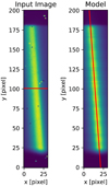 |
Fig. 9. Curvature estimation for one spectral line. Left: rectified input image cut out from the wavelength calibration frame. The order trace yc(x) is marked in red. Right: best-fit model image. The extracted tilt is marked in red. We only fit a linear tilt here. Data come from ESO/CRIRES+ Fabry-Pérot interferometer. |
where x is column number, δy is the row y distance to the central line, and m is the order number. Figure 10 shows an example of the fitted tilt. This is a 2D polynomial fit, so we reconstruct the slit image shape even in parts of spectral orders without any emission lines in the input image. This step is crucial for detecting and removing outliers created by a failed fit to individual lines (e.g. due to a cosmic ray hit or a detector defect). Similar to the wavelength calibration, the choice of the degree of the fit should be adjusted depending on the instrument and density of useful emission lines. The same curvature is plotted on top of the input image in Fig. 11.
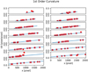 |
Fig. 10. Tilt variations per order (each panel is one order). Red pluses show the tilt determined for each individual emission line. The blue line is the 2D polynomial fit through all lines in all orders. Data from VLT/X-shooter (Vernet et al. 2011). |
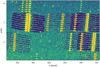 |
Fig. 11. Fragment of the input image used for the slit curvature determination (blue-yellow), with the recovered curvature (red) at line positions plotted on top. The red line is constructed from the final fit of the curvature and tracks the center of each spectral line along the slit. Data from VLT/X-shooter (Vernet et al. 2011). |
4. Wavelength calibration
The wavelength calibration of a grating spectrometer is based on the grating equation that connects the wavelength λ, the physical spectral order number m, the spacing between grooves δ, and the dispersion angle β:
 (33)
(33)
where α is the incidence angle, independent of the wavelength. The angular dispersion dλ/dβ is a function of m and reflection angle β (cos β). For modern echelle spectrometers, β occupies a small range of values centred on the blaze angle. The latter has typical values between 60 and 80 degrees. These result in a nearly constant dispersion for any given order. Thus, the relation between pixels and their wavelengths can be represented by a low-order polynomial. Polynomial orders of 3–5 are usually sufficient to reproduce the λ − β relation and to catch possible distortions introduced by the imaging system.
The determination of the polynomial coefficients requires a reference source with precision wavelengths assigned to emission (or absorption, as in the case of an absorption gas cell) lines. In this paper we leave out such crucial steps of wavelength calibration because of the determination of line centres and the use of a laser frequency comb (LFC) or Fabry-Pérot interferometer calibration source. We plan to revisit these aspects in a separate paper. In the meantime, we can find a detailed description of the calibration processing in the paper by Milaković et al. (2020).
Instead, we provide a summary of the procedure. A spectrum of a calibration source must be recorded with the spectrograph, with the spectral lines identified, their position measured in the detector coordinate system (pixels), and coefficients of polynomial regression determined. The spectral features of the reference source should preferably be evenly distributed across the spectral order to provide a homogeneous approximation and to minimise the maximum error. In this procedure, the main uncertainties are frequently coming from the erroneous identification of lines and measurements of their positions, as well as the use of blended or saturated lines.
It is a standard practice to create a specific reference line list for each instrument and setting, which includes the expected positions on the detector as well as the laboratory wavelength for each line. Once the solution is obtained, it can be recycled for later wavelength calibrations assuming that any line position changes will be much smaller than the line separation in dispersion direction and less than the order separation in cross-dispersion direction. An existing solution is then used as an initial guess for the next wavelength calibration.
The observed wavelength calibration spectrum is often extracted with a simple summation across the order. This is often sufficient since the flux level of a lamp tends to be much higher than that of a star. An example of the extracted image is shown in Fig. 12.
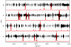 |
Fig. 12. Fragment with four partial orders of the input image used for the wavelength calibration (greyscale). The reference spectra (red) are shifted and scaled along the y axis so that they overlay their respective orders. Data come from La Silla/HARPS (Mayor et al. 2003). |
For many applications, instruments such as HARPS (Mayor et al. 2003), which are designed for high-stability, with no moving parts, and located in a stabilised environment, may use calibrations taken several hours before or after the science data. For extreme precision measurements as well as for general purpose instruments, the required repeatability is not reached this way. In these cases, an attached or simultaneous calibration is needed to complement the science data. Again, the reference solution can be used as an initial guess here.
Finally, the best-fit polynomial connecting position and wavelength can be determined. Valenti (1994) proposed using a 2D polynomial matching the dispersion variation within each order and between orders, as expected from the grating Eq. (33). The requirement of smooth variation (low-order polynomial) of dispersion and central wavelengths between spectral orders sets additional restrictions on the solution and helps to constrain the polynomial in parts of the focal plane void of emission lines in the calibration spectrum. An additional discussion of the polynomial degree and the dimensionality can be found below.
The polynomial fit involves a gradual improvement of the solution by rejecting the largest outliers in an iterative process. For this purpose, the residual Ri is defined not in the wavelength, but in velocity space:
 (34)
(34)
The process follows the conventional sigma-clipping algorithm and stops when no more statistically improbable outliers are found.
Starting from a reference solution and applying the outlier rejection described above, some lines may be unidentified. They can be recovered in an auto-identification phase. It finds all suitable unidentified peaks in the calibration, estimates their measured wavelength using the reference solution, and searches the reference lamp atlas for a possible match. With regard to ‘suitable’ lines, these are defined after a Gaussian fitting as having a full width half maximum (FWHM) in an acceptable range for the given instrument. The atlas is also checked for any possible blending of lines. Sigma-clipping and auto-identification phases can be repeated more than once to ensure the convergence of the overall procedure.
2D versus 1D wavelength polynomial
A reoccurring discussion when performing wavelength calibration is whether to use one 2D polynomial for all orders, or to use individual 1D polynomials for each order. The main arguments revolve around the ability of a 2D solution to minimise the maximum error in parts of the spectral orders without any reference lines versus the flexibility of the individual polynomial fit to each order, as illustrated in Fig. 13. In this example, based on the ThAr and LFC wavelength calibrations of the La Silla HARPS spectrometer, the differences between the 1D and the LFC solution reach in excess of 200 m s−1 in the peripheral parts of the detector, where a non-homogeneous distribution of the calibration lines is aggravated by the low signal. A similar 2D ThAr solution is generally close to the LFC result, except for the very ends of spectral orders.
 |
Fig. 13. Difference between the LFC wavelength solution and the ThAr-based 1D (left) and 2D (right) solutions for the red detector arm of the La Silla/HARPS spectrometer. Each vertical panel shows one spectral order with the longest wavelength order positioned at the bottom. The differences between ThAr and LFC solutions in m s−1 are plotted as red lines against detector pixels in the X-axis. LFC solutions were constructed separately for each spectral order. Blue crosses indicate the positions of the ThAr lines used for the construction of the wavelength solutions. In all cases, a 5th order polynomial was used for the dispersion direction. The 2D solution included an additional 3rd order cross-dispersion component as well as the corresponding cross-terms. |
This question is also closely related to the degree of polynomials used for the fit. A higher-order polynomial can fit the data better, but may also have larger variations from the true solution in places where data points are sparse. Ideally, we want to determine the best representation of the data with the fewest parameters possible. This is where the Akaike information criterion (AIC; Akaike 1974) is useful, as it combines the goodness of fit and the number of parameters into a single measure that can easily be compared between solutions. The AIC is defined as:
 (35)
(35)
where k is the number of parameters in the model and L is the likelihood. Since the least squares fit was used for the model the likelihood is given by the squared sum of the residuals (also known as χ2):
![Mathematical equation: $$ \begin{aligned} \ln {L} = - \frac{N}{2} \ln \left[\sum _{i=0}^N \left(R_i / c_{\rm light}\right)^2\right] + C, \end{aligned} $$](/articles/aa/full_html/2021/02/aa38293-20/aa38293-20-eq66.gif) (36)
(36)
where N is the number of lines, Ri is the residual as defined by Eq. (34), and C is a constant factor that we can ignore, since only the difference between AICs is relevant. Similarly, the clight factor could be removed since it only results in a constant, but is kept to make the values dimensionless.
Then we can simply use a grid search to find the best model, that is, the one with the lowest AIC. For the example of the HARPS ThAr wavelength calibration, the best AIC value is achieved with a 2D fit with degrees of 3 and 6 in dispersion and spatial direction respectively, see also Fig. 14 for an overview of the parameter space. The best 1D fit for this example is achieved with a polynomial of degree 2, although the AIC is larger than that of the 2D fit. Using HARPS with an LFC reveals the detector stitching as discussed by Coffinet et al. (2019). We can include corrections in the fit and find that the best fit has the degrees 9 and 7, respectively. Notably, the spatial degree remains similar, as the order number is separate from the detector pixels. As for ThAr, the 2D fit is preferred over the 1D fit.
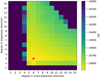 |
Fig. 14. AIC of different polynomials to the wavelength calibration with a ThAr gas lamp, based on the degree of the polynomial. The red diamond marks the best AIC (lower is better). All values above −16 000 are shown in the same colour to make the gradient more visible. Data from La Silla/HARPS. |
We can also compare the results of the different models with the LFC solution as an alternative reference. Figure 15 shows the distribution of the differences between the ThAr solutions and the LFC solution for HARPS. The two distributions are on the same order of magnitude, with the 1D solution being slightly wider. Notably, the 1D solution has more outliers, as shown by the larger standard deviation of the Gaussian. This is also visible in Fig. 16, as here the largest difference in each order is clearly larger in the 1D solution as compared to the 2D solution.
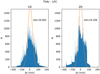 |
Fig. 15. Distribution of the difference between the ThAr wavelength solution and the LFC wavelength solution, evaluated for each point in all orders. The LFC solution is based on a 2D polynomial. There are more outliers beyond the limits of the histogram, which are not shown here. The orange dashed line, shows the Gaussian with the same mean and standard deviation as the whole distribution. Left: 1D ThAr solution, right: 2D ThAr solution. |
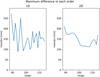 |
Fig. 16. Maximum difference between the ThAr wavelength solution and the LFC wavelength solution in each order. Left: 1D ThAr solution, right: 2D ThAr solution. The data from the red detector arm of HARPS at La Silla is showing spectral orders between 89 and 114. |
This result is exactly as we expected. We conclude that at least for the ThAr calibration, the 2D solution is more robust against missing data and possibly against errors in the line centre measurements.
5. Continuum normalisation
Robust continuum normalisation is a notoriously difficult task, even for well-behaved absorption line spectra. The few exceptions include cases when there is a well-matching synthetic spectrum available (as in the case of solar flux) or there are hot stars with very few spectral features. Among the various attempts to tackle this problem, better success was achieved with iterative schemes that fit the spectrum with a smooth function and gradually excluding points below the curve, until the distribution of data offsets from the constructed envelope becomes approximately symmetric and Gaussian. This, of course, does not guarantee that the normalised observed spectrum will match the synthetic spectrum. On the other hand, the correct synthetic spectrum is unknown to begin with and thus a heuristic approach is well motivated. The problem then becomes how to decide if a given point belongs to a spectral line and thus should be dropped from the fit. A power spectrum analysis, aimed at separating the spatial frequencies associated with spectral lines from the continuum envelope, does not help when considering individual spectral orders one at a time. The effect of the continuum ‘diving’ into the strong and broad lines remains just one of the issues.
5.1. Order splicing
In REDUCE, we take a single-order approach to the next level by extending the range of the sampled spatial frequencies by splicing several spectral orders into a single long spectrum. Splicing requires an existing wavelength solution so that adjacent spectral orders can be aligned, scaled, interpolated, and co-added in the overlap region as illustrated in Fig. 17. Combining the overlapping regions between neighbouring orders is complicated by the fact that the wavelengths associated with the pixels are different in the two orders. Firstly, we divide each order by the blaze function estimate, obtained, for example, from the master flat field. Even though the blaze estimate is not a perfect continuum, it is a good first step towards flattening the individual orders. We furthermore divide each order by its median in order to normalise everything to the same scale. We then determine the wavelength overlap and interpolate one order onto the wavelength grid of the other and vice versa. Finally, we co-add the values from both orders using a weighted sum with either linear weights or weights equal to the individual errors of each pixel1. The sum is given by:
 (37)
(37)
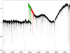 |
Fig. 17. Example of the spectral order splicing using the common wavelength scale. Before splicing we divide the signal by the blaze function derived from the flat field. We start from the order with the highest S/N, scale adjacent orders to achieve the best match in the overlap region and co-add the data with linear weights to avoid discontinuities. The black region to the right is already spliced. The scaling of the next order in line is shown in green. The scaled overlap region is shown in red. This example comes from the red detector of La Silla/HARPS. |
where xl, xr are the limits of the overlap region in pixels of the left order, Δx = xr − xl and σ’s are the uncertainties.  is the co-added value in the overlapping pixel x of the left order indicated by subscript l. Then
  is the overlapping part of the right order linearly interpolated onto pixel x of the left order.
The spliced spectrum still shows significant variations, but they are rather smooth. There are ‘waves’ in the shape of the upper envelope, which are primarily coming from the spectrum of the flat field calibration (the source of the blaze functions) and spectral sensitivity of the detector. These variations are to be fitted in the following step, but they are described by much lower spatial frequencies than the spectral lines. Even Hα looks ‘narrow’ in comparison to the broad level variations in Fig. 17. Uncertainties are spliced in the same fashion as the spectra to be used later in the fitting iterations. Once the splicing is completed, we sort the wavelengths and interpolate the spectrum onto an equispaced wavelength grid to have a better handle on the frequency spectrum in preparation for the continuum fitting.
5.2. Continuum fitting
We use a custom-made filtering routine for the construction of a smooth non-analytical function. The fitting function f(x) is defined in a such a way that it fits the data points well and at the same time has the least power in the highest spatial frequencies. The latter is achieved by restricting the minimisation of the averages of the first and the second derivatives with two regularisation terms:
![Mathematical equation: $$ \begin{aligned}&\sum _x \omega _x\left[f(x)-s(x)\right]^2+\Lambda _1\sum _x \left(\frac{df}{dx}\right)^2 \nonumber \\&\qquad \qquad \qquad +\Lambda _2\sum _x \left(\frac{d^2f}{dx^2}\right)^2= \mathrm{min} , \end{aligned} $$](/articles/aa/full_html/2021/02/aa38293-20/aa38293-20-eq70.gif) (38)
(38)
where s is the spectrum, x the wavelength point, ω is the weight/uncertainty, and Λ1 and Λ2 are regularisation parameters that control the stiffness of the fit and its behaviour at the end points. To be more specific, increasing Λ1 makes the solution more horizontal while a larger Λ2 ignores linear trends, but dampens high-frequency oscillations. The value of the two Λ parameters needs to be adjusted empirically. From Eq. (38), we construct a band-diagonal system of linear equations. Once the solution, f, is obtained we can start the iterations by constructing the histogram of s − f for all s values that are larger than f and estimating its width. We use a mirror reflection of the histogram in respect to 0 before fitting a Gaussian to it. The derived standard deviation is then used to reject points in s that are well below f. The procedure is repeated with the remaining points starting from a recomputed f. We also verify the consistency between the (spliced) uncertainties and the standard deviation of the distribution. The process reaches convergence (no more points are rejected) in about six to nine iterations. Examples of the final results are presented in Fig. 18. After completing the continuum fit on an equispaced grid, we interpolate the fit back to the initial wavelength grid of every spectral order. The same can be done with the observed spectrum, making individual orders look similar to the third panel from the top in Fig. 18. The gain is some increase in signal towards the ends of spectral orders. The downside is a possible loss of spectral resolution as well as distortions of the PSF due to focal plane aberrations and the interpolation procedures involved. Alternatively, it is possible to convert the ‘spliced’ continuum to a non-spliced version for each order using the splicing factors derived in Eq. (37). In this way, we do not modify the original data, which is important when, for instance, the science goals require the accurate determination of radial velocities or analysis of spectral line profiles.
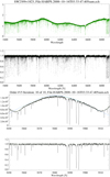 |
Fig. 18. Final result of the continuum fitting. Top: spliced spectrum is shown in green while the continuum is in black. Second panel: continuum-normalised spectrum. Two bottom panels: zoom on order #15 (absolute order 103). Third panel from the top: spliced spectrum is in black, the original (non-spliced) blaze function is in blue and the continuum fit is in green. The continuum-normalised order is shown in the bottom panel. Example comes from the red detector of La Silla/HARPS. |
 |
Fig. 19. Connection graph of the individual components. Diamond shapes represent nodes with raw file input, while square shapes only rely on data from previous steps. |
We conclude by re-iterating that the robust continuum normalisation of observed spectra is, indeed, impossible. What is described above may or may not give a satisfactory solution depending on S/N, spectral line width (e.g. due to stellar rotation), quality of the blaze functions, and many other factors. A good selection of the stiffness parameters requires some experience. Finally, the spectral format and the overlap between spectral orders are crucial for the splicing and for the whole procedure we developed. For instruments that leave gaps in the spectral coverage, continuum normalisation will remain more of an art than science.
6. Implementation
6.1. PyReduce
6.1.1. Introduction to PyReduce
PyReduce2 is a new open source implementation of the REDUCE pipeline written in Python with some C components. This new Python version is based on the existing REDUCE, which was written in IDL. Besides the change in the language most of the code has been rewritten from scratch and new features have been added. Notably, a fast and speed-optimised C-version of the extraction algorithm from Sect. 2 is included.
The data reduction in PyReduce is split into several individual steps, most of which produce calibration data for the science data extraction. The steps follow the methods described in the previous sections of this work, or in Paper I, and are listed as follows (PyReduce names in bold):
1. bias Creates the master bias frame, i.e. the intrinsic background from the detector without a light source.
2. flat Creates the master flat, i.e. the pixel sensitivity, from a continuum light source.
3. orders Traces the order locations on the detector and fits them with a polynomial.
4. curvature Determines the slit curvature along the orders, cf. Sect. 3.
5. scatter Estimates the scattered light background inside the orders from the signal between orders; see Sect. 6.1.3.
6. norm_flat Creates the normalised flat field from the master flat. This step also extracts the blaze functions.
7. wavecal Creates the wavelength calibration; see Sect. 4.
8. freq_comb Improves the wavelength solution by using a laser frequency comb (or similar); see also Sect. 4.
9. science Extracts the science spectrum from the science observations.
10. continuum Splices together the different orders into one long spectrum and fits the continuum level; see Sect. 5.
11. finalize Collects all the relevant data from the different steps into the final data product and adds helpful metadata information to the FITS header.
6.1.2. Using PyReduce
Once PyReduce is installed, the simplest way to use it is by calling the main method. This method only requires the location of the input files, instrument, observation target, and night to start. It locates all relevant files for this setup and performs all the steps defined above, if possible, using a predefined set of default parameters for the given instrument. These parameters are chosen to be viable in a wide range of applications, but users can, of course, set their own parameters.
To handle all kinds of different instruments, PyReduce uses instrument specific methods, that parse the FITS headers into the PyReduce standard format as described in Sect. 2, and identify files within the input folder. This makes it easy to apply PyReduce to many different instruments, and even extend it for new instruments if necessary.
The list of currently supported instruments is given in Table 1. Additional instruments can easily be added by providing the default parameters and a dictionary for the FITS header instruments-specific keywords.
Available test datasets, which are used for investigating the results of the data reduction.
6.1.3. Background scatter estimation
Depending on the spectrograph properties, such as scattered light, it can be necessary to estimate this kind of background from the inter-order regions on the detector and subtract it before extracting the spectra. The previous versions of REDUCE did this by extracting the order gaps, then linearly interpolating between the resulting spectra. In PyReduce, instead we perform a 2D polynomial fit to the pixel values between orders. This has the advantage that ghosts and other artifacts will not affect the background model. We illustrate this with data from the cs23-e2 spectrometer at McDonald 2.7m telescope. This instrument produces a very strong ghost image slowly crossing two spectral orders. The result of the new background estimate is shown in Fig. 20.
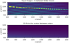 |
Fig. 20. Scattering background in the McDonald cs23-e2 spectrograph, zoomed in on the strong ghost. We note that the smooth 2D model of the background is not affected by the ghost feature. Both images are on the same colour scale. |
6.2. Example application: CRIRES+
CRIRES+ (Kaeufl et al. 2004) is an upgrade of the CRyogenic Infra-Red Echelle Spectrograph at the Very Large Telescope (VLT). What is most relevant in the context of this paper is the addition of a cross-disperser in form of a rotating wheel that carries six diffraction gratings, one for each of the YJHKLM bands. Thus CRIRES+ has become a cross-dispersed echelle spectrograph with several spectral orders (6–10, depending on the band) registered simultaneously by the new, larger and better detectors (3x2048x2048, HAWAII2RG). More information about CRIRES+ can be found in Dorn et al. (2016) or on the ESO instrumentation web site3.
Since the spectral format changed completely with the upgrade, the consortium and ESO re-developed the pipeline from scratch, keeping only a few relevant algorithms from the old CRIRES. The new optical design leads to a variable tilt of the slit image over the focal plane, reaching in some cases as far as ±4° from the vertical. This made obvious the need for an extraction algorithm that can handle this, spurring large parts of the work described in this paper. The slit image is close to but not exactly a straight line so we adopt a parabolic model for fitting the slit image, just as described in Sect. 2.6.
The C-implementation of the slit-decomposition algorithm is shared between PyReduce and the new ESO CRIRES+ pipeline. The routines that divide spectral orders into swaths and re-assemble the spectra are, however, written specifically for CRIRES+, using the ESO CPL library (McKay et al. 2004).
Thereby, the slit-decomposition described in Sect. 2 is now part of the ESO framework for data reduction system (DRS) development. Work is ongoing to include these algorithms into ESO’s High-level Data Reduction Library (HDRL) in order to make them more easily available to other instruments.
6.3. Example application: X-shooter
X-shooter (Vernet et al. 2011) is a medium resolution slit spectrograph at the VLT. The slit image of X-shooter shows clear and variable curvature (see Fig. 21), which makes this an excellent test case for our new extraction algorithm. The native X-shooter DRS (Modigliani et al. 2010) uses either interpolation for transforming spectral orders from detector coordinates into a rectangle in the wavelength-slit position plane or a 2D over-sampling of the detector pixels followed by a quasi-slit integration. Both methods are known to have deficiencies. Here, for the demonstration of our method we selected a random swath of 240 columns of order 12 in the NIR arm of a high S/N spectrum of UX Ori (ESO program ID 084.C-0952). Figure 22 shows a comparison of the input image and the model that is created by the extraction algorithm. The differences between the observation and the model are small (as shown in the bottom panel), matching the noise estimates except for a few cosmic ray hits and a bad pixel. Figure 23 shows the extracted 1D spectrum for this swath in comparison with the optimal extraction result of the X-shooter DRS and a simple vertical summation. We see excellent agreement between the two optimal extractions with slightly higher resolution (deeper lines) produced by our pipeline.
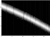 |
Fig. 21. Selected region of an X-shooter spectrum of UX Ori (fragment of order 12 in the NIR arm). Vertical dashed lines mark the central position of absorption spectral features highlighting the tilt. The grey-scale image is shown in log scale for better visibility. |
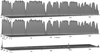 |
Fig. 22. Comparison of the detector image Ex, y (top) to the model Sx, y (middle) based on tilted slit decomposition algorithm. The differences are shown at the bottom. We note that cosmic ray hits such as the one around column 150 disappear in the model. |
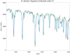 |
Fig. 23. Comparison of extracted spectra of UX Ori obtained with three different extraction methods. Native X-shooter DRS optimal extraction is shown in green. Our tilted slit-decomposition extraction is in black and a simple vertical summation is shown in blue. Spectral lines in our extraction appear somewhat deeper compared to the green spectrum. The vertical summation clearly degrades spectral resolution and misses about 2% of the flux. |
7. Conclusions
In the era of large and extremely large telescopes and instruments with price tags of tens of millions of Euros it is important not to forget the calibrations and data reduction procedures that assure they are on par with the ambitions of the coming generation of astronomical facilities. In this work, we describe previously unpublished algorithms and tools that address important steps in the data processing for modern spectroscopic instruments.
We developed, implemented, and tested novel algorithms for reducing astronomical observations with cross-dispersed slit echelle spectrometers. The central place in this suite of algorithms is occupied by a slit decomposition algorithm that is capable of handling tilted and curved slit images. We present the mathematical formulation of the problem and an efficiently optimised implementation that is crucial due to the computationally intensive nature of the problem. Tests and practical applications show excellent results in terms of preservation of the spectral resolution and the S/N of the extracted spectra. The algorithm is also robust against cosmic ray hits and isolated detector defects. An implementation in C was integrated in the ESO CRIRES+ DRS, ESO CPL library, and in our IDL and Python versions of the REDUCE package. These packages are publicly available. Some of the presented algorithms can by developed further, for example, in modeling the PSF-asymmetry in fibre-fed spectrometers such as ESO HARPS and ESPRESSO. We leave this topic for a future work.
As the spectra in each order come from different pixels they are independent measurements.
Acknowledgments
This work would not be possible without interaction within the CRIRES+ consortium, and with the ESO DRS group. We are very thankful to the ESO archive that provided many of the raw and reduced data used for testing and benchmarking for this paper. Finally, crucial financial support was provided by the Knut and Alice Wallenberg Foundation in form of the scholarship for one of the authors and the Russian Federation grant for the project “Study of Stars with Exoplanets” (Grant 075-15-2019-1875). PyReduce makes use of Astropy (http://www.astropy.org), a community-developed core Python package for Astronomy (Astropy Collaboration 2013, 2018).
References
- Akaike, H. 1974, IEEE Trans. Autom. Control, 19, 716 [NASA ADS] [CrossRef] [MathSciNet] [Google Scholar]
- Astropy Collaboration (Robitaille, T. P., et al.) 2013, A&A, 558, A33 [NASA ADS] [CrossRef] [EDP Sciences] [Google Scholar]
- Astropy Collaboration (Price-Whelan, A. M., et al.) 2018, AJ, 156, 123 [Google Scholar]
- Bolton, A. S., & Schlegel, D. J. 2010, PASP, 122, 248 [NASA ADS] [Google Scholar]
- Coffinet, A., Lovis, C., Dumusque, X., & Pepe, F. 2019, A&A, 629, A27 [NASA ADS] [CrossRef] [EDP Sciences] [Google Scholar]
- Cornachione, M. A., Bolton, A. S., Eastman, J. D., et al. 2019, PASP, 131, 124503 [NASA ADS] [CrossRef] [Google Scholar]
- Cui, B., Ye, Z. F., & Bai, Z. R. 2008, Acta Astron. Sin., 49, 327 [Google Scholar]
- Cushing, M. C., Vacca, W. D., & Rayner, J. T. 2004, PASP, 116, 362 [NASA ADS] [CrossRef] [Google Scholar]
- Dorn, R. J., Follert, R., Bristow, P., et al. 2016, SPIE Conf. Ser., 9908, 99080I [Google Scholar]
- Horne, K. 1986, PASP, 98, 609 [NASA ADS] [CrossRef] [EDP Sciences] [Google Scholar]
- Kaeufl, H. U., Ballester, P., Biereichel, P., et al. 2004, SPIE Conf. Ser., 5492, 1218 [Google Scholar]
- Kerschbaum, F., & Müller, I. 2009, Astron. Nachr., 330, 574 [NASA ADS] [CrossRef] [Google Scholar]
- Lenzen, F., Scherzer, O., & Schindler, S. 2005, A&A, 443, 1087 [NASA ADS] [CrossRef] [EDP Sciences] [Google Scholar]
- Marsh, T. R. 1989, PASP, 101, 1032 [NASA ADS] [CrossRef] [Google Scholar]
- Mayor, M., Pepe, F., Queloz, D., et al. 2003, Messenger, 114, 20 [Google Scholar]
- McKay, D. J., Ballester, P., Banse, K., et al. 2004, SPIE Conf. Ser., 5493, 444 [NASA ADS] [Google Scholar]
- Milaković, D., Pasquini, L., Webb, J. K., & Lo Curto, G. 2020, MNRAS, 493, 3997 [CrossRef] [Google Scholar]
- Modigliani, A., Goldoni, P., Royer, F., et al. 2010, SPIE Conf. Ser., 7737, 773728 [Google Scholar]
- Petersburg, R. R., Ong, J. M. J., Zhao, L. L., et al. 2020, AJ, 159, 187 [CrossRef] [Google Scholar]
- Piskunov, N. E., & Valenti, J. A. 2002, A&A, 385, 1095 [NASA ADS] [CrossRef] [EDP Sciences] [Google Scholar]
- Quirrenbach, A., Amado, P. J., Caballero, J. A., et al. 2016, SPIE Conf. Ser., 9908, 990812 [Google Scholar]
- Tikhonov, A. N., & Arsenin, V. Y. 1977, Solutions of ill-posed problems, xiii+258 (Washington, D.C.: John Wiley & Sons, New York: V. H. Winston & Sons), Translated from the Russian, Preface by translation editor Fritz John, Scripta Series in Mathematics [Google Scholar]
- Valenti, J. A. 1994, PhD Thesis, University of California, Berkeley, USA [Google Scholar]
- Vernet, J., Dekker, H., D’Odorico, S., et al. 2011, A&A, 536, A105 [NASA ADS] [CrossRef] [EDP Sciences] [Google Scholar]
- von Littrow, O. 1863, Sitzungsberichte der k. Akad. d. Wiss., mathem.-naturwiss. Klasse, XLVII Band. 47 Abt. 2 [Google Scholar]
- Zechmeister, M., Anglada-Escudé, G., & Reiners, A. 2014, A&A, 561, A59 [NASA ADS] [CrossRef] [EDP Sciences] [Google Scholar]
All Tables
Available test datasets, which are used for investigating the results of the data reduction.
All Figures
|
Fig. 1. Distribution of the first three swaths in an order. Each swath is overlapped by two other swaths (except for the first and last swath), so that each pixel is contained in two swaths. The swaths are combined into the final spectrum using linear weights with the central pixels having the most weight. |
| In the text | |
|
Fig. 2. Top: input image with selected order (dashed line) and two adjacent orders. Bottom: image packed for slit decomposition with the discontinuous order trace (dashed line). |
| In the text | |
|
Fig. 3. Schematic presentation of the subgrid sampling of the slit illumination function L and the corresponding structure of the ω tensor. On the top is an example of a slit illumination function aligned for column x. L is set on a subpixel scale v (shown at the bottom panel) that may shift relative to the detector pixels from one column to the next. For three pixels in this column centred at row y we show the structure of the corresponding section of |
| In the text | |
|
Fig. 4. Surface view of a 2D |
| In the text | |
|
Fig. 5. Surface view of ω⊤ × ω projection for a fixed x. The result is a symmetric square matrix with a dimensionality of ν. |
| In the text | |
|
Fig. 6. Schematic view of the product of ωTω for a fixed value of x. The result is a squared and symmetric matrix of order (Ny + 1) × O + 1 where Ny is the height of the packed swath. The outer side of the ‘squares’ on the main diagonal is O + 1. The squares overlap by one row or column. The offset from the top left corner is determined by the central line: a yc of zero implies vmin = 0. The in and out elements are the footprints of the first and the last subpixels that fall in a given detector pixel x, y. A central line offset of zero would set in = 1 and out = 0. All elements outside the main diagonal boxes are zero. The values inside a box are known explicitly as shown on the sketch. |
| In the text | |
|
Fig. 7. Schematic view of ‘ideal’ monochromatic images of a slit projected onto a detector by a non-Littrow spectrometer. Black squares represent spectrometer pixels. The dashed line traces the centre of a spectral order and the blue boxes show the idealised footprints of slit images. We note that by design the centre of the spectral order and the sides of a slit image intersect at the pixel column boundaries of the detector. |
| In the text | |
|
Fig. 8. Slit decomposition uncertainties. The top four panels show the 2D image of the data as registered by CARMENES (Ex, y in equations), the model reconstructed using the deduced P and L functions (Sx, y) and their difference. The difference image on the right of the 2nd row was multiplied by the bad pixel mask constructed during the decomposition and shows residual ripples with an amplitude of ∼12.5 counts. The next four panels show the recovered spectrum (P) and slit illumination function (L) on the left. Scattered dots are the actual data points aligned with the order centre and divided by the extracted spectrum. Green pluses show rejected (masked) pixels. The right panels compare uncertainty estimates assuming Poisson statistics for the whole swath (histogram) as well as for each column (right panel in the second row from the bottom). The latter compares S/N for each column x based on the shot noise only and on the observations-model discrepancy. The bottom panel compares our extraction (in green) with the standard CARMENES pipeline (in black). The black line was shifted to the right by 1 pixel for visibility. |
| In the text | |
|
Fig. 9. Curvature estimation for one spectral line. Left: rectified input image cut out from the wavelength calibration frame. The order trace yc(x) is marked in red. Right: best-fit model image. The extracted tilt is marked in red. We only fit a linear tilt here. Data come from ESO/CRIRES+ Fabry-Pérot interferometer. |
| In the text | |
|
Fig. 10. Tilt variations per order (each panel is one order). Red pluses show the tilt determined for each individual emission line. The blue line is the 2D polynomial fit through all lines in all orders. Data from VLT/X-shooter (Vernet et al. 2011). |
| In the text | |
|
Fig. 11. Fragment of the input image used for the slit curvature determination (blue-yellow), with the recovered curvature (red) at line positions plotted on top. The red line is constructed from the final fit of the curvature and tracks the center of each spectral line along the slit. Data from VLT/X-shooter (Vernet et al. 2011). |
| In the text | |
|
Fig. 12. Fragment with four partial orders of the input image used for the wavelength calibration (greyscale). The reference spectra (red) are shifted and scaled along the y axis so that they overlay their respective orders. Data come from La Silla/HARPS (Mayor et al. 2003). |
| In the text | |
|
Fig. 13. Difference between the LFC wavelength solution and the ThAr-based 1D (left) and 2D (right) solutions for the red detector arm of the La Silla/HARPS spectrometer. Each vertical panel shows one spectral order with the longest wavelength order positioned at the bottom. The differences between ThAr and LFC solutions in m s−1 are plotted as red lines against detector pixels in the X-axis. LFC solutions were constructed separately for each spectral order. Blue crosses indicate the positions of the ThAr lines used for the construction of the wavelength solutions. In all cases, a 5th order polynomial was used for the dispersion direction. The 2D solution included an additional 3rd order cross-dispersion component as well as the corresponding cross-terms. |
| In the text | |
|
Fig. 14. AIC of different polynomials to the wavelength calibration with a ThAr gas lamp, based on the degree of the polynomial. The red diamond marks the best AIC (lower is better). All values above −16 000 are shown in the same colour to make the gradient more visible. Data from La Silla/HARPS. |
| In the text | |
|
Fig. 15. Distribution of the difference between the ThAr wavelength solution and the LFC wavelength solution, evaluated for each point in all orders. The LFC solution is based on a 2D polynomial. There are more outliers beyond the limits of the histogram, which are not shown here. The orange dashed line, shows the Gaussian with the same mean and standard deviation as the whole distribution. Left: 1D ThAr solution, right: 2D ThAr solution. |
| In the text | |
|
Fig. 16. Maximum difference between the ThAr wavelength solution and the LFC wavelength solution in each order. Left: 1D ThAr solution, right: 2D ThAr solution. The data from the red detector arm of HARPS at La Silla is showing spectral orders between 89 and 114. |
| In the text | |
|
Fig. 17. Example of the spectral order splicing using the common wavelength scale. Before splicing we divide the signal by the blaze function derived from the flat field. We start from the order with the highest S/N, scale adjacent orders to achieve the best match in the overlap region and co-add the data with linear weights to avoid discontinuities. The black region to the right is already spliced. The scaling of the next order in line is shown in green. The scaled overlap region is shown in red. This example comes from the red detector of La Silla/HARPS. |
| In the text | |
|
Fig. 18. Final result of the continuum fitting. Top: spliced spectrum is shown in green while the continuum is in black. Second panel: continuum-normalised spectrum. Two bottom panels: zoom on order #15 (absolute order 103). Third panel from the top: spliced spectrum is in black, the original (non-spliced) blaze function is in blue and the continuum fit is in green. The continuum-normalised order is shown in the bottom panel. Example comes from the red detector of La Silla/HARPS. |
| In the text | |
|
Fig. 19. Connection graph of the individual components. Diamond shapes represent nodes with raw file input, while square shapes only rely on data from previous steps. |
| In the text | |
|
Fig. 20. Scattering background in the McDonald cs23-e2 spectrograph, zoomed in on the strong ghost. We note that the smooth 2D model of the background is not affected by the ghost feature. Both images are on the same colour scale. |
| In the text | |
|
Fig. 21. Selected region of an X-shooter spectrum of UX Ori (fragment of order 12 in the NIR arm). Vertical dashed lines mark the central position of absorption spectral features highlighting the tilt. The grey-scale image is shown in log scale for better visibility. |
| In the text | |
|
Fig. 22. Comparison of the detector image Ex, y (top) to the model Sx, y (middle) based on tilted slit decomposition algorithm. The differences are shown at the bottom. We note that cosmic ray hits such as the one around column 150 disappear in the model. |
| In the text | |
|
Fig. 23. Comparison of extracted spectra of UX Ori obtained with three different extraction methods. Native X-shooter DRS optimal extraction is shown in green. Our tilted slit-decomposition extraction is in black and a simple vertical summation is shown in blue. Spectral lines in our extraction appear somewhat deeper compared to the green spectrum. The vertical summation clearly degrades spectral resolution and misses about 2% of the flux. |
| In the text | |
Current usage metrics show cumulative count of Article Views (full-text article views including HTML views, PDF and ePub downloads, according to the available data) and Abstracts Views on Vision4Press platform.
Data correspond to usage on the plateform after 2015. The current usage metrics is available 48-96 hours after online publication and is updated daily on week days.
Initial download of the metrics may take a while.